Embed Size (px)
Citation preview
F a c u l t a d d e C i e n c i a s
GRADIENTES ECOLÓGICOS Y DISTRIBUCIÓN DE COMUNIDADES DE PECES EN RÍOS DE MONTAÑA:
DE LA ECOLOGÍA A LA CONSERVACIÓN; DE LOS PIRINEOS A LOS ANDES
ECOLOGICAL GRADIENTS AND FISH ASSEMBLAGE DISTRIBUTION IN MONTAINOUS STREAMS:
FROM ECOLOGY TO CONSERVATION; FROM THE PYRENEES TO THE ANDES
Ibon Tobes Sesma

F a c u l t a d d e C i e n c i a s
GRADIENTES ECOLÓGICOS Y DISTRIBUCIÓN DE COMUNIDADES DE PECES EN RÍOS DE MONTAÑA: DE LA ECOLOGÍA A LA CONSERVACIÓN; DE LOS PIRINEOS A LOS ANDES
ECOLOGICAL GRADIENTS AND FISH ASSEMBLAGE DISTRIBUTION IN MONTAINOUS
STREAMS: FROM ECOLOGY TO CONSERVATION; FROM THE PYRENEES TO THE ANDES
Memoria presentada por D. Ibon Tobes Sesma para aspirar al grado de Doctor por la Universidad de Navarra
El presente trabajo ha sido realizado bajo mi dirección en el Departamento de Biología Ambiental y autorizo su presentación ante el Tribunal que lo ha de juzgar. Pamplona, 16 de Mayo de 2016
Dr. Rafael Miranda Ferreiro (Director)

Πάντα ῥεῖ
Todo fluye
Ἡράκλειτος ὁ Ἐφέσιος
Heráclito de Éfeso

AGRADECIMIENTOS
ACKNOWLEDGMENTS

Este manuscrito representa solo una pequeña parte de lo que estos años de trabajo han significado para mi, ya que “el producto final de esta tesis doctoral no es este documento, sino toda la vida que desborda”. Y aunque la investigación científica ha sido la vertebradora de la experiencia, son las personas que han llenado estos años las que han hecho que todo el esfuerzo haya valido la pena. Espero haberos mostrado mi agradecimiento más hallá de estas palabras.
Esta tesis doctoral ha sido posible gracias al apoyo y amistad de Rafael Miranda Ferreiro, a quien nunca podré agradecerle lo suficiente el haber confiado en mi. Gracias por haberme dado la oportunidad de embarcarme en esta aventura y por acompañarme. Gracias por soñar las Américas y compartirlas conmigo.
Gracias al Departamento de Biología Ambiental de la Universidad de Navarra, por el apoyo, los cafés, las ideas, las barcaboas y las risas. Sin duda os habéis convertido en una de mis familias, mi familia científico-académica. Y también gracias a la Universidad de Navarra y a la Asociación de Amigos por haber confiado en mi y haberme brindado el apoyo financiero para la realización de la tesis.
Gracias también a todas las personas que han formado parte del trabajo de esta tesis con su consejo, apoyo, paciencia, sudor y tiempo.
Pero si hay alguien a quien debo estar especialmente agradecido es a mi familia, ya que a ellos les debo todo lo que soy. Mila esker, Aitatxo, Amatxo eta Iñigo. Eskerrik asko, Aitatxi eta Amatxi. Esker mila osaba, izeba, lehengusu eta lehengusiñei.
“Gu sortu ginen enbor beretik sortuko dira besteak”
Esta tesis doctoral es una colección de manuscritos en diferentes estados de publicación, cada uno de los cuales constituye un capítulo. Los manuscritos se reproducen íntegros y en el idioma en el que fueron publicados o enviados para su publicación, incluyendo siempre un resumen en castellano. Los artículos publicados han sido reproducidos con el permiso de las editoriales.
En cumplimiento de la normativa para la presentación de tesis doctorales en la Facultad de Ciencias de la Universidad de Navarra se incluyen los siguientes apartados en castellano: (1) un Resumen integrador del contenido de la tesis doctoral; (2) una Introducción general que sitúa el trabajo realizado en su contexto teórico, planteando los Objetivos de la tesis doctoral; (3) una Discusión general, y (4) un apartado de Conclusiones generales.
RESUMEN GENERAL GENERAL ABSTRACT ................................................................ 13
INTRODUCCIÓN GENERAL GENERAL INTRODUCTION .............................................. 19
CAPÍTULO 1ST CHAPTER ........................................................................................... 49
Diagnóstico de la integridad de los ecosistemas fluviales en la Reserva de la Biosfera de Ordesa‐Viñamala, en los Pirineos centrales de España
Diagnosing stream ecosystem integrity in the Ordesa‐Viñamala Biosphere Reserve, central Spanish Pyrenees Journal of Applied Ichthyology, 32(1), 229‐239 (2016)
CAPÍTULO 2ND CHAPTER ........................................................................................... 71
Patrones de distribución espacial de las comunidades de peces en relación a los macroinvertebrados y a las condiciones ambientales de los ríos del piedemonte Andino Amazónico de Colombia
Spatial distribution patterns of fish assemblages relative to macroinvertebrates and environmental conditions in Andean piedmont streams of the Colombian Amazon Inland Waters 6(1), 89‐104
CAPÍTULO 3RD CHAPTER ......................................................................................... 101
Relaciones longitud‐peso de diecises peces del río Hacha y sus afluetes (cuenca Amazónica, Caquetá, Colombia)
Length‐weight relationships of sixteen freshwater fishes from the Hacha River and its tributaries (Amazon Basin, Caquetá, Colombia) Journal of Applied Ichthyology, 28(4), 667‐670
CAPÍTULO 4TH CHAPTER ......................................................................................... 111
Distribución de las comunidades de peces y los patrones ambientales a lo largo de la cuenca del río Suaza (Colombia): desde el Parque Nacional Natural Cueva de los Guácharos hasta los territorios de su cuenca baja
Fish assemblage distribution and environmental patterns in the Suaza River Basin (Colombia): from the Cueva de los Guacharos National Park to the downstream territories
CAPÍTULO 5TH CHAPTER ......................................................................................... 131
Relaciones biométricas de los peces del río Suaza (Departamento de Huila, Colombia)
Biometric relationships of freshwater fishes of the Suaza River (Huila Department, Colombia) Enviado a Acta Ichthyologica et Piscatoria
CAPÍTULO 6TH CHAPTER ......................................................................................... 143
Ecología y patrones de distribución de las comunidades de peces del río Alto Madre de Dios, Perú: implicaciones del conocimiento en la conservación y gestión
Ecology and distribution patterns of fish assemblages in the Alto Madre de Dios River, Perú: implications of knowledge in the conservation and management
CAPÍTULO 7TH CHAPTER ......................................................................................... 167
Relaciones de longitud‐peso de los peces del río Alto Madre de Dios (Reserva de la Biosfera del Manu, Perú)
Length‐weight relationships of freshwater fishes of the Alto Madre de Dios River (Manu Biosphere Reserve, Peru) Enviado a Journal of Applied Icthyology
DISCUSIÓN GENERAL GENERAL DISCUSSION ......................................................... 175
CONCLUSIONES GENERALES GENERAL CONCLUSIONS ........................................... 205
BIBLIOGRAFÍA REFERENCES ................................................................................... 209
13
RESUMEN
ABSTRACT

14
15
Resumen
La humanidad se enfrenta en el siglo XXI a una crisis ambiental sin precedentes. Perdemos hábitats y biodiversidad, y con ellos, innumerables servicios esenciales que los ecosistemas nos proveen. Y entre todos los ecosistemas del planeta son los ríos los que se encuentran especialmente amenazados. Esto es debido a que integran las alteraciones que ocurren tanto en sus riberas y cauces como en todo el territorio de su cuenca de drenaje. Es esta cualidad de colectores la que los hace especialmente vulnerables a los impactos humanos. Y debido a esta degradación a gran escala a la que los ríos están expuestos, los organismos que los habitan irremediablemente sufren sus consecuencias. No es de extrañar entonces que los peces de agua dulce estén catalogados como el grupo de vertebrados más amenazado del planeta. A la luz de este escenario resulta prioritario desarrollar estrategias de protección que garanticen la conservación de estos hábitats y su biodiversidad. Sin embargo, muchos de estos ríos y especies que aspiramos a salvaguardar son en muchos casos desconocidos para la ciencia, lo cual representa un importante obstáculo para su gestión. Este vacío de conocimiento es especialmente significativo en el neotrópico, donde también se concentra la mayor diversidad de peces de agua dulce del planeta. Desgraciadamente, estos territorios tan biodiversos están actualmente expuestos a grandes amenazas que están destruyendo sus hábitats. La suma de ambos factores destaca a los Andes Tropicales como una región especialmente biodiversa y gravemente amenazada cuya conservación debe ser prioritaria. Sin embargo, cualquier acción de gestión ambiental debe estar basada y respaldada por un completo conocimiento ecológico que garantize su idoneidad. Es por ello que resulta prioritario llevar a cabo estudios científicos integrales que nos faciliten toda la información biológica posible. Con la intención de paliar tan apremiante necesidad de conocimiento científico, esta tesis doctoral aspira a evaluar la eficacia y utilidad de una metodología de muestreo para completar estudios ecológicos en ecosistemas fluviales, especialmente centrada en el estudio de los peces. La metodología busca ser versátil, integradora y sencilla, y ha sido puesta a prueba en distintos contextos biogeográficos. Así, se analizaron cinco cuencas fluviales (dos en los Pirineos y tres en los Andes Tropicales) llevando a cabo muestreos de pesca eléctrica, recolección de macroinvertebrados acuáticos, caracterizaciones del hábitat fluvial y aplicación de índices de calidad ambiental. Los resultados obtenidos fueron usados para analizar los procesos ecológicos que configuran los ríos a escala de cuenca y tramo y su influencia sobre la distribución de las comunidades de peces. También se evaluó la integridad de los ecosistemas fluviales intentando comprender las consecuencias de los impactos humanos sobre la biota y las problemáticas subyacentes. Una de las estrategias más habituales para la protección de ecosistemas y especies es la creación de áreas protegidas. Las de Reservas de la Biosfera aspiran a garantizar la conservación de la biodiversidad y promover el desarrollo sostenible de las comunidades humanas que en ellas habitan. Pero la escasez de información biológica disponible y la falta de estudios que evalúen la efectividad de estos espacios protegidos pueden estar obstaculizando la exitosa gestión y conservación de los ríos y los peces dentro de sus territorios. Los resultados obtenidos en esta tesis doctoral señalan que, aunque algunas Reservas de la Biosfera estén cumpliendo parcialmente su función protectora, se está descuidando su gestión, y sus planes de acción no se adaptan y no asimilan la información científica disponible para proteger los ríos y garantizar su conservación. Aunque las campañas de muestreo efectuadas aplicando la metodología mencionada nos han permitido conocer mejor los peces y los ríos y diagnosticar su integridad ecológica, la limitación de visitar una sola vez cada lugar impide comprender en profundidad su compleja realidad. Sin embargo, la información obtenida nos permite señalar como prioritaria la protección de las cabeceras de los Andes Tropicales. Son zonas muy bien conservadas, responsables de proveernos de una gran
16
variedad de servicios ecosistémicos y albergan una gran cantidad de especies de peces endémicos para cada una de las cuencas. Además, debido a la influencia que los impactos humanos ya están teniendo sobre estos hábitats, debemos llevar a cabo estudios ecológicos que nos permitan conocer los ríos en su estado previo a las alteraciones humanas para así contar con unas condiciones de referencia en la que basar las políticas de gestión y restauración. Esta demanda de conocimiento pone en evidencia la necesidad de seguir llevando a cabo campañas de muestreo de carácter exploratorio, que aspiren a cubrir los amplios vacíos de conocimiento aún existentes y que faciliten el trabajo a la biología de la conservación. El conocimiento de la biodiversidad en un territorio es el primer paso para protegerla, ya que, no valoramos lo que no conocemos, y no protegemos lo que no valoramos.
17
Abstract
River ecosystems integrate all the changes that occur throughout the territory of their basin and for this is why they are among the most threatened and altered ecosystems in the world. This loss of habitat has direct consequences on the organisms inhabiting them. Freshwater fish are the most threatened group of vertebrates on the planet. Therefore, we must prioritize their protection implementing effective management strategies capable to ensure the conservation of riverine habitats and species. Nevertheless, there is a big gap of knowledge involving these ecosystems and biota, hindering their management. This lack of knowledge is especially significant in the Neotropics, where the greatest diversity of freshwater fish of the planet water is found. Unfortunately, these highly biodiverse areas are exposed to great threats that are destroying their habitats. These facts point out the Tropical Andes as a particularly biodiverse but seriously threatened region whose conservation should be prioritized. However, management plans must be based on appropriate ecological studies, providing reliable biological information and guaranteeing the development of appropriate conservation strategies. In the light of this critical knowledge gap, this thesis aims to evaluate the effectiveness of a sampling methodology that aspires to be versatile, inclusive and simple, testing it in different biogeographic contexts. Thus, five river basins (two in the Pyrenees and three in the Tropical Andes) were analyzed conducting electrofishing surveys, collecting aquatic macroinvertebrates, characterizing river habitat and applying environmental quality indices. One of our main goals was to study the freshwater ecological processes and its influence on the distribution of fish communities. Additionally, we evaluated the integrity of river ecosystems, trying to understand the consequences of human impacts on the biota. One of the most common strategies for the protection of ecosystems and species is the creation of protected areas. The Biosphere Reserves aspire to protect biodiversity and promote the sustainable development of the communities inhabiting them. Nevertheless, the scarcity of available biological information and the lack of studies that evaluate the effectiveness of these protected areas may be hindering the successful management and conservation of rivers and fish inside them. Our results point out that, although some Biosphere Reserves are partially fulfilling their protective function, their management strategies should be revised and their action plans adapted to the new available scientific information. Our sampling campaigns provided us with a better understanding of the ecology of poorly known rivers and fish, and the methods proved to reliability to diagnose ecological integrity. Nevertheless, due to time and budged limitations, we could only visit once each of the basins, hindering our interpretation of their complex reality. However, the obtained data allows us to emphasize the urge of prioritizing the protection of the headwaters of the Tropical Andes. They still remain very well preserved, they provide invaluable and irreplaceable ecosystem services and host a large number of fish species endemic to each of the basins. In addition, given the increasing anthropogenic impacts threatening these ecosystems, it is mandatory to delve into ecological studies to understand the natural reference conditions of these rivers, necessary to the appropriate development of management policies and restoration. This urge for knowledge highlights the necessity to continue with exploratory sampling campaigns, aspiring to cover the large knowledge gaps we are facing, and to guarantee the effectivity of the conservation biology. Biodiversity and ecology knowledge are the foundations for protecting nature.

18
19
INTRODUCCIÓN
INTRODUCTION

20
21
“Anyone who thinks that you can have infinite growth on a planet with finite resources is either a madman or an economist”
Sir David Attenborough
Bienvenidos al Antropoceno
El planeta en el que vivimos, el único en todo el universo conocido capaz de
albergar vida, está cada día un poco más cerca de su colapso (Meadows, Meadows, &
Randers, 1992). En pleno siglo XXI, la era de la información, nadie se sorprenderá ante
esta dramática afirmación, y muy pocos se atreverán a negarla. Una sentencia
convertida en una verdad a gritos, una perogrullada, un lapidario veredicto ante el cual
no solo no nos estremecemos, sino que apenas hace mella en nuestro cotidiano suicidio.
La historia de la Tierra ha estado marcada desde su comienzo por catastróficos
eventos (glaciaciones e impactos de asteroides), que alteraron drásticamente las
condiciones ambientales a escala planetaria, dando lugar a extinciones masivas que se
llevaron por delante al 99,99% de las especies que alguna vez habitaron el planeta
(Raup, 1991). Son estos cambios a escala global los que determinan el fin de una era
geológica y el comienzo de la siguiente, los que marcamos en rojo en el calendario
“mil-milenario” de la historia de la Tierra. Sin embargo, en la actualidad, somos los
seres humanos los que hemos hendido la última de estas muescas en la superficie
terrestre. Tenemos el dudoso honor de haber inaugurado nuestra propia era geológica, el
Antropoceno, en la cual el catastrófico evento que pone en riesgo a toda la vida del
planeta es nuestra existencia viral, nuestro cancerígeno Progreso (Zalasiewicz et al.,
2011). Y no solo dejaremos nuestra huella en la litosfera en forma de una capa
estratigráfica de plástico, emblema de nuestro tiempo (Zalasiewicz et al., 2011), hemos
demostrado que somos mucho más eficientes que los meteoritos y las glaciaciones a la
hora de exterminar formas de vida. Tenemos el récord. Somos responsables de la tasa de
extinción de especies más drástica de la historia de la Tierra: se estima que podemos
estar perdiendo 8700 especies al año, 24 especies al día (Convention on Biological
Diversity, 2010). Somos los responsables de la desaparición de seres vivos únicos e
irrepetibles, verdugos inconscientes de miles de formas de vida que ni siquiera hemos
llegado a conocer (Kemp, 2015). Bastante dramático, ¿verdad?
22
Los ríos en la crisis global
“Hay mucha agua sin vida en el universo, pero en ninguna parte hay vida sin agua”
Sylvia A. Earle
Esta categórica afirmación encumbra al agua como el más vital de los recursos
naturales. Sin embargo, solo el 3% de toda el agua del planeta es dulce (Shannon,
2008). Es la que hay, y hay la que es. No hay más. Y estamos dilapidándola y
contaminándola como si nunca se fuera a agotar. A este desfalco1 hay que sumarle el
innegable, impredecible e inminente efecto que el cambio climático puede tener en su
distribución y disponibilidad, lo que nos deja un escenario incierto y poco halagüeño
(Meybeck, 2003).
Aproximadamente un 80% de la población del planeta se encuentra en una
situación de alto riesgo debido a la vulnerabilidad de sus recursos hídricos (el agua
empieza a escasear o está envenenada, o ambas) siendo los países más desfavorecidos
los más expuestos a esta amenaza (Vörösmarty et al., 2010). Las estimaciones señalan
que, en la actualidad, el 65% del agua dulce continental ya se encuentra en una situación
de vulnerabilidad moderada o grave (Vörösmarty et al., 2010).
Los ríos son las venas de nuestro planeta, el sistema circulatorio de la Tierra, y
su función en los ciclos biogeoquímicos (carbono, hidrógeno, oxígeno) es esencial para
garantizar la continuidad de la vida tal y como la conocemos (Galy, Peucker-Ehrenbrink
& Eglinton, 2015). Al igual que nuestras arterias, los ríos distribuyen materiales y
nutrientes esenciales para la vida a lo largo de los ecosistemas por los que circulan
(Verhoff, Melfi, & Yaksich, 1980). Así como nuestras venas se encargan de recoger los
desechos indeseados de nuestro organismo para eliminarlos, los ríos desempeñan una
función análoga para los ecosistemas terrestres que los rodean (Aylward et al., 2005).
Además de encajar todos los golpes que directamente les infringimos sobre sus cauces y
riberas, son los sumideros que sufren, integran y acumulan el daño causado por el
hombre en toda su cuenca (Allan, 2004). Por este motivo, por su estrecha relación y
dependencia con su entorno, los ecosistemas fluviales son en la actualidad los más
expuestos y vulnerables frente a los impactos ambientales causados por el hombre
1 Apropiación indebida de bienes o dinero ajenos por parte de la persona que ha de custodiarlos

23
(Karr, 1981). Son posiblemente los hábitats más amenazados del planeta (Gozlan et al.,
2010).
Este escenario resulta especialmente dramático para los organismos que habitan
los ríos, prisioneros en su propio hogar, más seriamente comprometidos que cualquier
otro grupo animal o vegetal (Ricciardi & Rasmussen, 1999). Las consecuencias son
obvias: masivas pérdidas de biodiversidad dulceacuícola a nivel mundial (Dudgeon et
al., 2006). La desaparición de especies es sin duda una terrible tragedia, un daño
irreparable que debemos paliar con urgencia. Pero no solo estamos perdiendo formas de
vida únicas, sino que somos igualmente responsables de una masiva “defaunación” o
merma en la abundancia de las poblaciones de animales: puede que ya hayamos perdido
un 25% de todos los animales del planeta (Dirzo et al., 2014).
Los servicios de los ecosistemas fluviales y sus principales amenazas
Además de ser el único hogar para una infinidad de organismos vivos, los
ecosistemas fluviales nos proveen de unos servicios ecosistémicos esenciales e
irremplazables sin los cuales nuestra supervivencia estaría seriamente amenazada
(Pimentel et al., 1997; Aylward et al., 2005; Brauman et al., 2007):
Nos aprovisionan de agua dulce: para beber, para uso doméstico, para regar
nuestros cultivos, para completar procesos industriales y para generar energía eléctrica.
También nos proporcionan vías de transporte y navegación y albergan muchos
organismos acuáticos que aprovechamos para una gran variedad de usos.
Cumplen un servicio de regulación: mantienen la calidad y cantidad de agua, nos
protegen ante crecidas e inundaciones y controlan la erosión a través de interacciones
entre agua/tierra.
Tienen una importante función de soporte: por un lado, su rol en los ciclos de
nutrientes y en la producción primaria es esencial (fertilidad de llanuras de inundación)
y, por otro, dotan de resiliencia a los ecosistemas.
Poseen valores culturales y estéticos intangibles y nos proporcionan servicios
recreativos (rafting, kayak, senderismo y pesca deportiva).
24
Sin embargo, todos estos servicios esenciales de los que somos absolutamente
dependientes, están empezando a ser cada vez más disfuncionales debido al uso
desmesurado y desconsiderado que de ellos hacemos (Brauman et al., 2007). Damos por
sentado que los ríos siempre nos van a proveer de agua en cantidad y calidad y que los
peces de los que nos alimentamos nunca se agotarán. Olvidamos todos los desechos que
vertemos en sus aguas tan pronto como la corriente las arrastra lejos de nuestra vista.
Pero nuestros actos tienen consecuencias, y aunque les demos la espalda, aunque
sigamos pasándole la factura de nuestros excesos a los ecosistemas naturales “que todo
soportan”, la magnitud e intensidad de nuestros desmanes está sobrepasando la
capacidad de carga del planeta (Holling, 1986). Estamos sobrepasando la resiliencia de
los ecosistemas abocándolos al colapso (Hughes, 2003). Ignoramos “convenientemente”
que ni todo el dinero y la tecnología del mundo podrán jamás reemplazar los servicios
vitales que nos regalan (d'Arge et al., 1997).
Esta sobrecarga de impactos antrópicos es especialmente intensa y preocupante
para los ecosistemas fluviales debido a su papel como colectores (Allan, 2004). A
continuación se presentan las seis principales amenazas con las que estamos
comprometiendo la integridad de los ecosistemas fluviales y los servicios que nos
brindan (Allan & Flecker, 1993; Lammert & Allan, 1999; Abell, 2002; Dudgeon et al.,
2006; Olden et al., 2010; Vörösmarty et al., 2010):
Cambios de usos del territorio y degradación de la cuenca
El principal impacto a nivel de cuenca es causado por la deforestación del
territorio drenado y su transformación en tierras de cultivo o pastos para ganadería. Las
consecuencias son: alteraciones severas en el ciclo hidrológico (fuertes sequías e
inundaciones); erosión, sedimentación y colmatación de los cauces; alteraciones en la
carga de nutrientes (pérdida de los aportes naturales y entrada de agroquímicos y
contaminación orgánica); pérdida de hábitats y biodiversidad asociada.
Contaminación
El masivo vertido de aguas residuales no tratadas (urbanas e industriales)
envenena los ríos. A este impacto directo hay que sumarle la llegada de grandes
cantidades de agroquímicos (abonos y pesticidas) arrastrados por las lluvias desde los
campos de cultivo.
25
Represas y embalses
La creciente demanda energética ha provocado la proliferación de los proyectos
hidroeléctricos en todo el planeta. Cada represa construida cercena la unidad de los
ecosistemas fluviales, interrumpe su conectividad y compromete seriamente su
integridad. Altera los ciclos hidrológicos, el transporte de sedimentos y nutrientes y
obstaculiza las vitales migraciones de muchos peces.
Sobrepesca
Los peces de agua dulce son la principal fuente de proteínas para muchas
sociedades rurales de países tropicales. La insaciable colonización de nuevos territorios
y el exponencial aumento de las poblaciones humanas dependientes de este recurso
alimenticio están agotando las pesquerías continentales debido a la sobreexplotación a
la que están sometidas.
Especies exóticas
La invasión de especies alóctonas representa una grave amenaza para los
organismos autóctonos y para la integridad de sus ecosistemas. La llegada de estas
especies exóticas, casi siempre facilitada por los seres humanos (intencionada o
accidentalmente), es una de los motivos principales de extinción de especies a nivel
mundial.
Cambio climático
Es un hecho de sobra constatado que el clima del planeta está cambiando de
forma drástica, posiblemente como nunca antes había ocurrido en la historia de la
Tierra. Las implicaciones a nivel global son inciertas, pero parece una tendencia
generalizada que allí donde las lluvias ya son escasas lo serán aún más y que
aumentarán allí donde ya son abundantes. La capacidad de los ecosistemas para soportar
y sobreponerse a las perturbaciones podría mitigar los efectos adversos del cambio
climático. Sin embargo, la degradación de los hábitats, sumada al escenario de cambio
global, acentuarán de forma sinérgica los problemas anteriormente expuestos.
26
Lo que sabemos que no sabemos pero que deberíamos saber
“Ser consciente de la propia ignorancia es un gran paso hacia el saber.”
Benjamin Disraeli
Vivimos en la era del conocimiento, un tiempo en el que la información, las
ideas y la creatividad se han reivindicado como renovadores e inagotables recursos
inmateriales, importantes agentes de cambio capaces de traer prosperidad y bienestar a
las sociedades humanas (Duderstadt, 1997). Conscientes de que estamos inmersos en un
contexto de cambio global cubierto por un velo de incertidumbre, estimamos,
modelamos, proyectamos e intentamos imaginarnos en el futuro para empezar cuanto
antes a prepararnos y adaptarnos al nuevo escenario global (Sala et al., 2000). Basamos
nuestras predicciones en todo el conocimiento acumulado lo largo de la historia, lo
compartimentamos para poder abarcarlo y entenderlo, y lo volvemos a ensamblar para
construir modelos capaces de integrar tantas variables como podamos controlar
(Norgaard, 2010). Y es este reto el que nos enfrenta a nuestras carencias. Cegados por
un optimismo científico y tecnológico, muchas veces nos olvidamos de lo limitado de
nuestro entendimiento en muchos ámbitos que pueden resultar vitales para nuestra
supervivencia (Gibbons, 1994). Aspiramos a salvaguardar la integridad del planeta,
queremos garantizar la funcionalidad de los ecosistemas y proteger a sus hábitats y
habitantes, pero para ello resulta prioritario e indispensable que conozcamos en
profundidad y de forma holística aquello que buscamos preservar (Jenkins, 1988).
Debemos conocer para conservar. Necesitamos información ecológica y
taxonómica precisa en la que basar nuestras estrategias de adaptación y gestión,
conocimiento que garantice la idoneidad de las medidas adoptadas. Estos vacíos de
conocimiento representan importantes obstáculos para la gestión de los ecosistemas y su
conservación: ¿cuánto territorio es necesario proteger para garantizar su viabilidad a
largo plazo? ¿Con qué medidas de protección? ¿Cuáles son los hábitats prioritarios? ¿Y
cuáles las estrategias de gestión adecuadas? (Thieme et al., 2007). Esta información
resulta especialmente crítica cuando trabajamos con especies y hábitats vulnerables y
amenazados, ya que una mala decisión puede resultar irreparable (Dejean et al., 2011).
27
Especialmente notable es el vacío de conocimiento que existe para los peces de
agua dulce, y aunque puede que representen el 25% de las especies de vertebrados del
planeta, son sin duda los vertebrados menos estudiados e históricamente relegados a un
segundo plano (Winemiller, Agostinho, & Caramaschi, 2008). Como para la mayoría de
los grupos animales, su diversidad es máxima en latitudes tropicales, y especialmente
abundante en las grandes cuencas de Suramérica (Moulton & Wantzen, 2006). Esta
carencia de conocimiento científico es especialmente significativa para los ecosistemas
fluviales de los Andes tropicales donde todavía existen muchas especies de peces
desconocidas para la ciencia y para las cuales apenas existe información relevante
(Barthem et al., 2003). No existe información taxonómica o ecológica, desconocemos
sus requerimientos ambientales, su relación con el medio en el que habitan, sus áreas de
distribución o su grado de amenaza. Tampoco conocemos sus procesos de dispersión,
las estructuras metapoblacionales, la viabilidad de sus poblaciones actuales, sus
adaptaciones y dependencia en los regímenes naturales de caudal e inundación y mucho
menos su tolerancia y respuesta a las cambios ambientales ejercidos por las presiones
antrópicas (Allan & Flecker, 1993; Abell, 2002; Maldonado-Ocampo et al., 2005; Lujan
et al., 2013). Esto se debe a que aún existen amplios territorios inexplorados para la
ciencia, ríos a los que jamás ha llegado un ictiólogo o un ecólogo fluvial (Wheeler,
Raven, & Wilson, 2004; Junk & Piedade, 2004).
Además, muy pocas veces somos los científicos los primeros en llegar a “terra
incognita”. Es demasiado habitual que a los biólogos nos precedan los impactos
humanos y que los paisajes que estudiamos ya hayan sido alterados por la mano del
hombre. Sin embargo, resulta esencial que conozcamos las condiciones previas a estos
impactos y que estudiemos los ecosistemas antes de que hayan sufrido grandes
alteraciones (Bailey et al., 1998). Son estas condiciones naturales las que usaremos
como referencia para futuros planes y estrategias de conservación, y son también las
condiciones que debemos aspirar a preservar pues son las que garantizan la
funcionalidad y la integridad de los ecosistemas así como la supervivencia de los
organismos que en ellos habitan (Pardo et al., 2012).
No obstante, nuestra escala de influencia sobre el medio ambiente es planetaria y
posiblemente no exista un solo ecosistema prístino en la Tierra que no haya sufrido
alteraciones debidas a nuestra presencia, aunque sea de forma indirecta (Sala et al.,
28
2000). Este escenario es especialmente dramático en Europa, el viejo continente; viejo
por lo ajado y maltratado. Después de siglos de constante y creciente presión antrópica,
después de soportar el nacimiento y apogeo de la revolución industrial, no existe un solo
rincón del continente que no haya sufrido alteraciones de la mano del hombre, y la gran
mayoría de sus paisajes actuales son el resultado de esta convivencia, por lo que hace
siglos que se perdieron para siempre las condiciones de referencia de los ecosistemas
europeos originales (Kalis, Merkt & Wunderlich, 2003). Sin embargo, aún existen en el
planeta grandes extensiones de territorio que apenas han sido alteradas, especialmente
en los trópicos, donde la presión ejercida sobre el medio tiene una historia reciente;
ecosistemas donde el Progreso no ha llegado y que albergan la mayoría de la
biodiversidad del planeta (Ceballos et al., 2009). Por lo que aún hay esperanza. Puede
que todavía estemos a tiempo de actuar y frenar el acelerado deterioro ambiental al que
están expuestos estos recónditos paisajes. Podemos adelantarnos a la llegada de nuestros
impactos y evitar sus nefastas consecuencias. Debemos priorizar y proteger estos
grandes reservorios naturales que apenas han sido alterados y conservar así sus
intangibles valores (Harris, Jenkins, & Pimm, 2005).
Los Andes Tropicales: amenazas y oportunidades
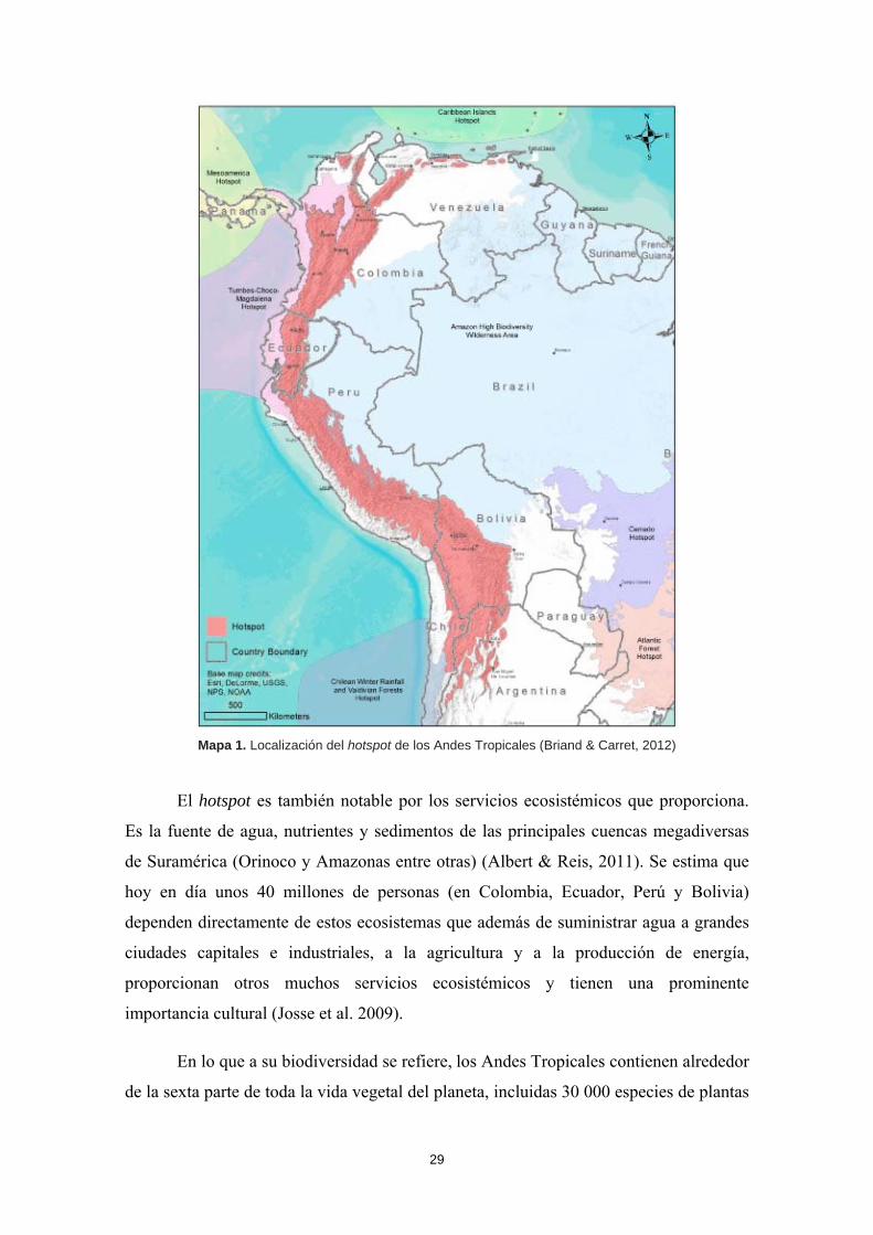
Los Andes tropicales son uno de los puntos calientes o hotspots para la
conservación de la biodiversidad a nivel mundial. Se trata de ecosistemas cuya
protección es prioritaria debido a la elevadísima diversidad de especies endémicas que
albergan y al hecho de estar enfrentándose a una acelerada pérdida de hábitats (Tabla 1).
Este hotspot está considerado como el más biodiverso de los 35 hotspots mundiales
(Myers et al., 2000). Abarca la Cordillera de los Andes de Venezuela, Colombia,
Ecuador, Perú, Bolivia y las porciones tropicales septentrionales de Argentina y Chile
(Mapa 1). Su altitud oscila entre los 500 m hasta más de 6000 m y ocupa un total de
158.3 millones de hectáreas, un área tres veces el tamaño de España (Briand & Carret,
2012).
29
Mapa 1. Localización del hotspot de los Andes Tropicales (Briand & Carret, 2012)
El hotspot es también notable por los servicios ecosistémicos que proporciona.
Es la fuente de agua, nutrientes y sedimentos de las principales cuencas megadiversas
de Suramérica (Orinoco y Amazonas entre otras) (Albert & Reis, 2011). Se estima que
hoy en día unos 40 millones de personas (en Colombia, Ecuador, Perú y Bolivia)
dependen directamente de estos ecosistemas que además de suministrar agua a grandes
ciudades capitales e industriales, a la agricultura y a la producción de energía,
proporcionan otros muchos servicios ecosistémicos y tienen una prominente
importancia cultural (Josse et al. 2009).
En lo que a su biodiversidad se refiere, los Andes Tropicales contienen alrededor
de la sexta parte de toda la vida vegetal del planeta, incluidas 30 000 especies de plantas
30
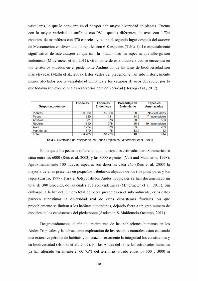
vasculares, lo que lo convierte en el hotspot con mayor diversidad de plantas. Cuenta
con la mayor variedad de anfibios con 981 especies diferentes, de aves con 1.724
especies, de mamíferos con 570 especies, y ocupa el segundo lugar después del hotspot
de Mesoamérica en diversidad de reptiles con 610 especies (Tabla 1). Lo especialmente
significativo de este hotspot es que casi la mitad todas las especies que alberga son
endémicas (Mittermeier et al., 2011). Gran parte de esta biodiversidad se encuentra en
los territorios situados en el piedemonte Andino donde las tasas de biodiversidad son
más elevadas (Malhi et al., 2008). Estos valles del piedemonte han sido históricamente
menos afectados por la variabilidad climática y los cambios de usos del suelo, por lo
que todavía son excepcionales reservorios de biodiversidad (Herzog et al., 2012).
Tabla 1. Diversidad del hotspot de los Andes Tropicales (Mittermeier et al., 2011)
En lo que a los peces se refiere, el total de especies estimadas para Suramérica se
sitúa entre las 6000 (Reis et al. 2003) y las 8000 especies (Vari and Malabarba, 1998).
Aproximadamente 100 nuevas especies son descritas cada año (Reis et al. 2003) la
mayoría de ellas presentes en pequeños tributarios alejados de los ríos principales y los
lagos (Castro, 1999). Para el hotspot de los Andes Tropicales se han documentado un
total de 380 especies, de las cuales 131 son endémicas (Mittermeier et al., 2011). Sin
embargo, a la luz del número total de peces presentes en el subcontinente, estos datos
parecen subestimar la diversidad real de estos ecosistemas fluviales, ya que
probablemente se limitan a los hábitats altoandinos, dejando fuera a un gran número de
especies de los ecosistemas del piedemonte (Anderson & Maldonado-Ocampo, 2011).
Desgraciadamente, el rápido crecimiento de las poblaciones humanas en los
Andes Tropicales y la subsecuente explotación de los recursos naturales están causando
una extensiva pérdida de hábitats y amenazan seriamente la integridad los ecosistemas y
su biodiversidad (Brooks et al., 2002). En los Andes del norte las actividades humanas
ya han alterado seriamente el 60–75% del territorio situado entre los 500 y 3000 m
31
(Etter & van Wyngaarden, 2000). Este acelerado crecimiento de las poblaciones está
aumentando exponencialmente la demanda de agua y está provocando graves problemas
de contaminación debido a los vertidos de aguas residuales urbanas e industriales,
comprometiendo gravemente las reservas y recursos hídricos (Postel & Mastny, 2005).
Otra de las principales amenazas es la deforestación masiva y los cambios de
usos de suelo en los territorios más fértiles y aptos para la ganadería y agricultura
(Herzog et al., 2012). Los productivos valles interandinos de Colombia y Ecuador son
los que históricamente han estado más expuestos a la explotación de sus recursos y a la
alteración de sus ecosistemas naturales (Josse et al., 2009). En la actualidad, el nuevo
frente de conquista y explotación se sitúa en el “arco de la deforestación”, el cual se
expande desde la periferia de la cuenca amazónica hacia su interior; desde el sur de
Brasil creciendo hacia el norte; y descendiendo desde el piedemonte Andino-
Amazónico y extendiéndose hacia el corazón de selva, hacia el este (Aldrich et al.,
2012). A su paso, el bosque desaparece, y deja tras de sí bastas superficies ganaderas y
monocultivos de soja y palma africana que se pierden en el horizonte (Ceballos et al.,
2009).
La proliferación de proyectos hidroeléctricos a lo largo de toda la cordillera
representa también una importante amenaza a la integridad de sus ecosistemas,
especialmente para los ecosistemas fluviales (Lees et al., 2016). La construcción de
represas es responsable de cambios irreparables e impredecibles que afectan tanto las
cabeceras sobre las que impactarán directamente, como a las cuencas bajas que sufrirán
importantes cambios en sus ciclos hidrológicos (Finer & Jenkins, 2012).
Todas estas problemáticas se verán agravadas por el efecto sinérgico del cambio
climático. Los modelos climáticos sugieren futuros incrementos de temperatura en los
Andes del orden de 2–3ºC para la mitad del siglo XXI y de 3–4ºC para finales del siglo
XXI (Marengo et al. 2011). Este escenario de cambio afectará severamente los ciclos de
lluvias, disminuyendo la precipitación en el altiplano y aumentando hasta un 20–25% en
ambas vertientes de los Andes (Amazónica y Pacífica) (Malhi et al., 2008).
32
Las cabeceras y los valles del piedemonte Andino
Ante este dramático escenario es necesario actuar con premura para paliar la ya
avanzada degradación de los Andes Tropicales. Para ello resulta fundamental fijar
prioridades y dirigir nuestros esfuerzos para que resulten lo más efectivos y eficientes.
Una posible línea de trabajo para asegurar la conservación de la biodiversidad andina
puede ser garantizar la integridad de aquellos ecosistemas que todavía no han sido
alterados y que albergan las mayores, mejores y únicas comunidades animales y
vegetales, así como la mayor variedad de ecosistemas prístinos.
Esta línea de acción apunta directamente a las cabeceras y piedemonte andino,
nacientes de la compleja red fluvial cuyas intrincadas venas se extienden por todo el
subcontinente. Aunque representen una pequeña porción del territorio de estos grandes
sistemas fluviales, las cabeceras andinas aportan más de un 40% de toda el agua que
alimenta al Amazonas y al Orinoco, entre otros muchos (Goulding, Barthem & Ferreira,
2003). Por ello, la pérdida de estas fuentes pondría en grave riesgo la integridad de estas
grandes cuencas megadiversas, y desconocemos las consecuencias del efecto dominó
que podría desencadenar para todos los ecosistemas que de ellas dependen (Malhi et al.,
2008). Por lo tanto, la conservación de las cabeceras de los ríos andinos es prioritaria
para garantizar la integridad y funcionalidad de los principales ecosistemas fluviales de
Suramérica (Junk & Piedade, 2004).
Las cabeceras y valles del piedemonte andino son también zonas de transición
entre los ecosistemas de montaña y llanura, y son por ello uno de los territorios más
biodiversos del continente (Thieme et al., 2007; Romero, Cabrera, & Ortiz, 2008) y
albergan una gran diversidad de organismos y ecosistemas únicos e irremplazables
(Herzog et al., 2012). Los endemismos son una característica común en las naciente
montañosas de los ríos, donde los gradientes altitudinales y climáticos restringen la
dispersión de las especies (Boulton & Boyero, 2008). Estas cabeceras y los valles de las
cuencas de los Andes Tropicales pueden ser considerados como islas, aislados unos de
otros por la elevación de la cordillera y por las particulares condiciones ambientales a
las que aparecen estrechamente relacionadas unas pocas especies (Schaefer & Arroyave,
2010). Este aislamiento salvaguarda la diversidad genética, un factor clave para la futura
evolución de las especies (Allan & Flecker, 1993). Este fenómeno de aislamiento y
especiación es notable en latitudes tropicales debido a la gran variedad de biomas que
33
existen en comparación a ríos similares en latitudes templadas (Boulton & Boyero,
2008). Aunque la diversidad piscícola adaptada a estos ecosistemas fluviales sea
muchísimo más baja que la que podemos encontrar en las zonas más bajas de las
cuencas, sus tasas de endemismo son altísimas (Tabla 1), con especies únicas para cada
una de las cuencas, lo que convierte a estos ecosistemas en hábitats únicos e
irremplazables (Schaefer et al., 2011).
Afortunadamente, debido en parte a su inaccesibilidad y su abrupta morfología,
todavía existen cuencas prácticamente prístinas a lo largo de la cordillera que apenas
han sido alteradas por la mano del hombre, ofreciendo esperanzadoras oportunidades
para la conservación (Etter & van Wyngaarden, 2000). Sin embargo, debido a su difícil
acceso y aislamiento, también son una de las regiones menos estudiadas de Suramérica,
siendo especialmente notable la falta de trabajos sobre ríos y peces (Menezes, 1996).
Áreas protegidas
Ante la crisis ambiental a la que nos enfrentamos debemos actuar sin demora y
empezar a proteger de forma estricta y efectiva ecosistemas, paisajes, hábitats y
especies. Sin embargo, la falta de conocimiento a la que nos enfrentamos plantea un
importante dilema: ¿deberíamos seguir estudiando en profundidad los ecosistemas para
poder tomar las decisiones adecuadas, o deberíamos actuar inmediatamente usando
estrategias que han demostrado su efectividad en otros territorios?
Los territorios designados para la conservación son habitualmente establecidos
en base a la disponibilidad de un inventario de paisajes a escala regional, de los patrones
biogeográficos de la biota terrestre o a la necesidad específica de proteger especies
amenazas, normalmente, especies terrestres. Uno de los criterios tradicionales para
seleccionar territorios a proteger es elegir áreas que alberguen una alta biodiversidad,
buscando garantizar su conservación a largo plazo (Giangrande, 2003). En
consecuencia, la falta de registros biogeográficos completos da lugar a la creación de
áreas de protección que excluyen hábitats o especies de interés, lo cual obstaculiza
notablemente su función principal, la conservación.
Esta falta de conocimiento es común para muchos de los espacios protegidos a
nivel mundial, y es demasiado habitual en América Latina (Junk & Piedade, 2004). No
34
existen estudios ecológicos que aborden los ecosistemas fluviales, y ni siquiera se
conocen las especies de peces que habitan los ríos protegidos (e.g., Myer et al., 2000).
Los peces son obviados demasiado a menudo en los planes de gestión, o en el mejor de
los casos, la información existente es escasa e incompleta (Pino-Del-Carpio et al.,
2011). Esta problemática resulta especialmente significativa para aquellos organismos
que carecen de importancia económica o que no tienen interés para la investigación
experimental, hablamos entonces de la inmensa mayoría de especies de peces que
habitan el neotrópico (Olden et al., 2010). Paradójicamente, tal y como s exponía
anteriormente, los peces de agua dulce son el grupo de vertebrados más amenazados del
planeta.
Además, los espacios de conservación son habitualmente creados para proteger
ecosistemas terrestres, sin tener muy en cuenta los ecosistemas fluviales (Herbert et al.,
2010). Esta desconsideración hacia los ríos y los peces hace que los territorios de las
áreas protegidas no sean congruentes con los patrones regionales de riqueza y
distribución de los organismos acuáticos. Es por ello que las áreas protegidas diseñadas
para la protección de los ecosistemas terrestres resultan habitualmente inadecuadas para
los ecosistemas fluviales (Barletta et al., 2010; Herbert et al., 2010).
Finalmente, en innegable el consenso internacional que considera las áreas
protegidas como figuras esenciales para la conservación de la biodiversidad en un
mundo cambiante y hostil (Gaston et al., 2008; Chessman, 2013). Sin embargo, vedar
completamente el acceso a grandes extensiones de territorio y aislarlas del mundo
exterior para protegerlas no parece una estrategia realista. Es por ello que existen una
gran variedad de figuras de protección ambiental más o menos restrictivas respecto al
uso que se puede hacer de sus territorios, y con diferentes encajes socio-ambientales
(Kemsey et al., 2012).
Reservas de la Biosfera
Una de las figuras de protección más interesantes y versátiles son las Reservas
de la Biosfera, creadas por la Organización de las Naciones Unidas para la Educación,
la Ciencia y la Cultura (UNESCO) en 1970 (UNESCO, 1970). Su figura fue concebida
para responder a una de las preguntas esenciales del mundo contemporáneo: ¿cómo
conciliar la preservación de la diversidad biológica y de los recursos naturales con su
35
uso sostenible? Según la definición de la UNESCO, son “zonas de ecosistemas
terrestres o costeros/marinos, o una combinación de los mismos, reconocidas en el
plano internacional como tales en el marco del Programa sobre el Hombre y la
Biosfera (MaB)” y son establecidas “para promover y demostrar una relación
equilibrada entre los seres humanos y la biosfera”. Así pues, las Reservas de la
Biosfera son áreas protegidas que integran los usos humanos, donde la conservación de
sus recursos y su aprovechamiento sostenible se presenta como un proyecto esencial.
Para conseguir un equilibrio y encaje territorial de sus funciones, se establece la
siguiente zonificación:
Zona núcleo: estrictamente protegidas, dedicadas a la conservación a largo plazo
de la diversidad biológica y los ecosistemas. Su uso se restringe a la investigación y
otras actividades poco perturbadoras (educación ambiental, etc.). Suelen coincidir con
espacios protegidos ya existentes, como los Parques Nacionales.
Zona de amortiguamiento: generalmente circundando o colindantes a las zonas
núcleo. Se destina a actividades compatibles con los objetivos de conservación de la
zona núcleo, ayudando a su protección. Se desarrolla investigación y se promueve la
formación científica, además de permitir actividades de educación ambiental, turismo y
recreación (siempre que no resulten lesivas para el medio).
Zona de transición: es considerada una zona de uso múltiple, en la que deben
fomentarse y desarrollarse formas de explotación sostenible de los recursos. Puede
comprender variadas actividades agrícolas, asentamientos humanos, y otros usos, donde
las comunidades locales, organismos de gestión, científicos, organizaciones no
gubernamentales, sector económico y otros interesados, trabajan conjuntamente en la
administración y desarrollo sostenible de los recursos de la zona.
Para el año 2013, la red mundial de Reservas de la Biosfera contaba ya con 651
espacios en 120 países distinguidos con esta figura de protección. Estos sitios aspiran a
ser una muestra de la biodiversidad del planeta y de cómo el hombre puede habitarlo de
forma sostenible (http://www.unesco.org/new/es/santiago/natural-sciences/man-and-
the-biosphere-mab-programme-biosphere-reserves/).
36
Diseñando una metodología de muestreo buena, bonita y barata
"La verdadera ignorancia no es la ausencia de conocimientos,
sino el hecho de negarse a adquirirlos"
Karl Popper
Establecido el marco teórico y ante la necesidad de conocer para proteger, es
hora de buscar una forma efectiva, poco costosa y rápida con la que llevar a cabo
estudios ecológicos que nos permitan conocer tan a fondo como sea posible los ríos y su
entorno, los peces y otros organismos que los habitan, su integridad y amenazas, y la
relación que existe entre todos estos elementos. Ante esta necesidad metodológica son
varias las preguntas que se nos plantean:
¿Se puede llevar a cabo un análisis integral de los ecosistemas fluviales con
medios y tiempo limitados?
¿Cómo distribuimos los puntos de muestreo para obtener una imagen
representativa de los distintos hábitats y comunidades biológicas?
¿Cuál es la información mínima necesaria que nos permite obtener una imagen
general del estado ecológico de los ríos y de su cuenca?
¿Qué herramientas nos permiten llevar a cabo una caracterización de hábitats y
diagnóstico ambiental de forma sencilla pero efectiva?
Selección de puntos de muestreo
A la hora de seleccionar los puntos de muestreo buscamos conseguir una red de
localizaciones que pudiera ser representativa de toda la cuenca fluvial. Es un trabajo que
se realiza “desde la oficina”, sobre el papel, basado en mapas e información ecológica,
sin conocer in situ el territorio.
Como criterio base, buscamos una separación significativa entre los segmentos
estudiados, estableciendo una distancia de unos 5 a 10 km entre los puntos
seleccionados, suficiente para detectar cambios en las características del río, pero no tan
alejados como para perdernos los cambios graduales en las condiciones ambientales y
37
en las comunidades biológicas (Karr, 1981). De forma complementaria, identificamos
posibles puntos de cambio de hábitat basados en la información geomorfológica y
territorial disponible para adaptar la distribución de las localidades a la variabilidad
ambiental: pendiente, altitud, tipología de cauces, características de la cuenca,
desembocadura de afluentes, presencia de impactos humanos, áreas protegidas, etc.
(Bain, Finn & Booke, 1985). Sin embargo, todo biólogo ambiental sabe que, aunque el
papel lo aguanta todo, al final es la naturaleza la que manda, por lo que las restricciones
de acceso o la viabilidad de muestrear los tramos seleccionados sobre el papel
habitualmente deben adaptarse a la realidad.
Análisis ecológico y diagnóstico ambiental
La cualidad integradora de los ríos los convierte en ecosistemas indicadores del
estado ecológico de todo el territorio (Valero, Álvarez, & Picos, 2015). Si conocemos
las condiciones de referencia, sus características naturales y las consecuencias que las
alteraciones antrópicas tienen sobre ellos, al llevar a cabo un estudio de su estado
ecológico podemos identificar la presencia de impactos, estimar su intensidad o grado
de afectación e incluso identificar el origen de dicho impacto (Infante et al., 2008).
Siguiendo esta lógica, el estudio de las comunidades de peces y
macroinvertebrados no solo nos da una información ecológica valiosa, sino que además,
se trata de sensibles indicadores de la calidad ambiental, por lo que pueden ser usados
llevar a cabo diagnósticos de la integridad de los ecosistemas (Fausch et al., 2002;
Johnson et al., 2007). Su uso como indicadores ambientales está ampliamente
reconocido y aplicado a nivel mundial (Friberg et al., 2011).
Sin embargo, para poder usar los peces y macroinvertebrados como
bioindicadores, es esencial que conozcamos cómo las condiciones ambientales naturales
configuran su distribución y abundancia a lo largo del río (Vannote et al., 1980;
Schlosser, 1991). Es totalmente necesario que usemos las condiciones de referencia
previas a cualquier impacto para establecer el estado base, así como tenemos que
conocer la tolerancia de las diferentes especies y comunidades ante diferentes tipos y
grados de alteración (Canton et al., 1984).
38
Estudio de las comunidades de peces: pesca eléctrica
En la actualidad, la pesca eléctrica es la técnica más ampliamente usada en todo
el mundo para llevar a cabo estudios de comunidades de peces de agua dulce (Bain,
Finn & Booke, 1985; Paller, 1996; Pusey et al., 1998; Survey, 2003; Bertrand, Gido, &
Guy, 2006; Angermeier & Davideanu, 2004). Se trata de un método de colecta no
selectivo que nos permite tener muestras representativas de toda la población de peces
en un tramo de río vadeable y estudiar sus abundancias y comunidades con bajo riesgo
de dañar a los individuos (Zalewski, 1985; Beaumont et al., 2002; Meador, McIntyre &
Pollock, 2003; Angermeier & Davideanu, 2004). Consiste en someter a las aguas a un
campo eléctrico creado por un generador de corriente que puede causar en los peces
electrotaxis (natación obligada), electrotétanosis (contracción muscular) y
electronarcosis (relajación muscular), lo que facilita su captura (Bertrand et al., 2006).
Es un método que permite una buena prospección de los tramos fluviales sin ocasionar
daños en la fauna presente en el rio, ya que los animales afectados por la corriente se
recuperan rápidamente (Survey, 2003). Además, es suficiente contar con un equipo
humando de dos a cuatro personas para poder completarlo exitosamente (Paller, 1996).
Existen diferentes metodologías para llevar a cabo prospecciones con pesca
eléctrica: los muestreos pueden ser cualitativos o cuantitativos; y la estimación de las
abundancias de peces pueden hacerse en base a la superficie muestreada (acotada o
libre; con una o varias pasadas) o en base al esfuerzo de muestreo (tiempo muestreado)
(Meador, McIntyre & Pollock, 2003). A la vista de las necesidades del presente
proyecto de investigación, con el tiempo disponible como máximo limitante y la
obtención de un inventario faunístico lo más completo posible como prioridad,
seleccionamos una metodología de muestreo cuantitativa, basada en capturas por unidad
de esfuerzo (CPUE) medidas por tiempo. Con la idea de optimizar el esfuerzo de
muestreo y extraer la máxima información que pueda ayudar a caracterizar la población
piscícola, se obtuvieron datos de relación de longitud-peso de los individuos.
Sin embargo, aunque nadie ponga en duda la efectividad de la técnica para
muestrear ríos en zonas templadas, existe mucha discrepancia sobre su efectividad en
los ríos neotropicales cuyas conductividades son significativamente más bajas (Allard et
39
al., 2014). Algunos estudios la consideran ineficiente en ríos de estas características
(Fisher & Brown, 1993; Penczack et al. 1997; Beaumont, 2002).
La efectividad de la pesca eléctrica depende principalmente de la conductividad
del agua, aunque la profundidad y anchura del río, por lo tanto, el volumen del cuerpo
de agua muestreado también influye en su eficacia (Allard et al., 2014). A
profundidades mayores a un metro y en ríos con más de 10 metros de ancho, o cuando
la conductividad es inferior a los 43 µs cm-1, los peces escapan con mayor facilidad
(Murphy & Willis, 1996). Sin embargo, funciona perfectamente para ríos pequeños
(<50 cm) y con conductividades superiores a los 43 µs cm-1 (Allard et al., 2014).
Otros autores mencionan que la baja temperatura del agua, las altas velocidades
de la corriente, la baja visibilidad (ya sea por la turbidez o por ser aguas torrentosas) y la
abundancia de refugios pueden mermar su efectividad (Zalewski, 1985). Además, es
posible que la sensibilidad de las especies de peces sea distinta dependiendo de su
comportamiento, morfología y fisiología (Reyjol, Loot & Lek, 2005). Un claro ejemplo
lo constituyen las especies nocturnas como los gymnotiformes y muchos siluriformes,
ambas abundantes en el neotrópico (Albert & Reis, 2011). Al estar ocultas durante el
día, aunque el campo eléctrico les afecte se quedan paralizadas dentro de sus refugios y
por ello son subestimadas.
Sin embargo, aunque la efectividad de la técnica pueda verse mermada en
determinadas circunstancias, existen también muchos estudios que aseguran que la
pesca eléctrica es perfectamente efectiva también en ríos neotropicales (Esteves &
Lobón-Cerviá, 2001; Bührnheim & Fernandes 2003; Lujan et al., 2013). Por ello, a
pesar de las posibles limitaciones, decidimos elegirla como técnica de muestreo y
ponerla a prueba personalmente.
Muestreo de macroinvertebrados acuáticos
El estudio de los macroinvetebrados, además de ofrecernos una relevante
información ecológica con un gran valor intrínseco, nos posibilita evaluar la integridad
de los ecosistemas acuáticos (Utz, Hilderbrand, & Boward, 2009). Su uso está
considerado como una de las mejores técnicas disponibles para diagnosticar la calidad
ambiental de los ecosistemas fluviales (Rosenberg & Resh, 1993; Bonada et al., 2006;
40
Friberg et al., 2011). Para su recolección, aplicamos el protocolo habitual de toma y
procesado de muestras para este tipo de estudios (Jaimez-Cuellar et al. 2002).
Para usar estas comunidades de invertebrados como indicadores de calidad
ambiental, la metodología seleccionada fue la propuesta por el Biological Monitoring
Working Party (BMWP) (Barbour et al., 1999). Se trata de la metodología más habitual
y que ha demostrado su fiabilidad después de haber sido aplicada por todo el mundo
(Thorne & Williams, 1997; Junqueira & Campos, 1998; Mustow, 2002).
Aunque el índice BMWP es una herramienta de gran utilidad, es totalmente
necesario que se base en un conocimiento integral y completo de la ecología de los
taxones usados como referencia (Johnson et al., 2007). Su validez depende de una
correcta ponderación con las condiciones de referencia, del estudio de la sensibilidad de
las diferentes familias ante las alteraciones y del conocimiento de su respuesta ante la
presencia de los impactos ambientales (Utz, Hilderbrand & Boward, 2009). Es por ello
que resulta indispensable contar con adaptaciones locales del índice, ajustadas en
función a las características ambientales de cada región. En nuestro caso utilizamos la
adaptación para la Península Ibérica, IBMWP (Alba Tercedor et al., 2002), y una
adaptación para ecosistemas neotropicales, el BMWP/Col (Roldán, 2003).
Caracterización ecológica e índices de calidad ambiental
Resulta esencial para interpretar los datos faunísticos conocer cuáles son los
factores ambientales o antrópicos que condicionan su distribución. Es por ello que la
metodología de muestreo incluyó un procedimiento de caracterización de hábitat que
analizaban las propiedades físico-químicas del agua (temperatura, conductividad, pH,
oxígeno disuelto, presencia de contaminantes) y las características hidromorfológicas de
los cauces (velocidad del agua, tipo de sustrato, anchura, profundidad, sombra)
(Armantrout, 1998).
Como herramienta diagnóstica complementaria a los índices bióticos basados en
las comunidades de macroinvetebrados, incluimos en la metodología varios índices de
calidad ambiental. Esto índices cuentan con una larga trayectoria histórica (Ott, 1978) y
son en la actualidad ampliamente aceptados y usados en todo el mundo (Pykh, Kennedy
& Grant, 2000). Nos aportan una información estandarizada de la integridad ecológica
41
de los ecosistemas, permitiéndonos comparar distintas localizaciones y facilitándonos la
identificación de zonas impactadas y su grado de alteración (Munne et al., 2003). La
facilidad con la que pueden ser aplicados sin conocimientos especializados, su bajísimo
coste y su versatilidad los han convertido en una metodología útil, sencilla y muy usada
(Chapman, 1996).
A la hora de elegir los índices más adecuados para obtener un diagnóstico
ambiental integral, buscamos índices complementarios que nos permitieran evaluar
distintos componentes del ecosistema fluvial, desde el cauce y los hábitats dentro del río
al estado de las riberas. Sin embargo, tal y como ocurre con los índices bióticos basados
en las comunidades de macroinvetebrados (Friberg et al., 2011) o peces (Karr, 1981),
estos índices requieren un conocimiento ecológico base que debe ser usado para calibrar
sus puntajes y adaptarlos a las diferentes realidades biogeográficas (Chapman, 1996). Es
por esto que los índices elegidos fueron aquellos que, además de haber demostrado su
solidez metodológica y valía como herramientas diagnósticas, pudieran ser aplicados en
lugares tan dispares como los estudiados en esta tesis doctoral. Así, elegimos el índice
QHEI (Rankin, 1989) para estudiar el hábitat fluvial, debido a su aplicabilidad en
diferentes contextos biogeográficos (An, Par & Shin, 2002; Arimoro, 2009; Beyene et
al., 2009; Song et al., 2015), y lo complementamos con el Índice de Hábitat Fluvial, IHF
(Pardo et al., 2002), desarrollado para la península ibérica, pero que cuenta con una
adaptación para ecosistemas andinos (Acosta et al., 2009). Por esta misma razón
seleccionamos el Índice de Calidad de Bosque de Ribera, QBR (Fornells, Solá &
Munné, 1998), desarrollado en España, pero adaptado también a ecosistemas de los
Andes (Acosta et al., 2009).
Presentación de casos y justificación
Con el objetivo de poner a prueba la metodología de muestreo y evaluar su
validez como herramienta de diagnóstico ambiental, el presente proyecto de
investigación pasó a su fase práctica. Para ello se seleccionaron cinco cuencas con
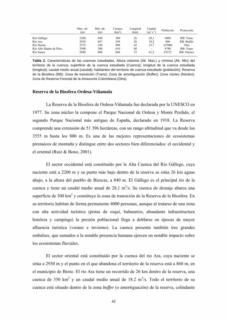
realidades muy distintas pero que comparten unas características comunes (Tabla 2).
Dos de las cuencas, el río Ara y el río Gállego, se encuentran en los Pirineos españoles.
Las otras tres se situan en los Andes tropicales, las cuencas de los ríos Hacha y Suaza,
en Colombia, y la cuenca del Alto Madre de Dios en Perú.
42
Max. alt.
(m) Min. alt.
(m) Cuenca (km2)
Longitud (km)
Caudal (m3 s-1)
Población Protección
Río Gállego 2200 840 300 26 28,1 4000 RB: Trans Río Ara 2930 867 350 26 18,2 900 RB: Buffer Río Hacha 2575 240 490 65 35,7 167000 Otra Río Alto Madre de Dios 3500 300 410 80 - 4790 RB: Trans Río Suaza 2840 800 660 35 41,2 47272 RB: Núcleo
Tabla 2. Características de las cuencas estudiadas. Altura máxima (Alt. Max.) y mínima (Alt. Min) del territorio de la cuenca; superficie de la cuenca estudiada (Cuenca); longitud de la cuenca estudiada (longitud); caudal medio anual (caudal); habitantes del territorio de cuenca estudiado (población); Reserva de la Biosfera (RB); Zona de transición (Trans); Zona de amortiguación (Buffer); Zona núcleo (Núcleo); Zona de Reserva Forestal de la Amazonía Colombiana (Otra).
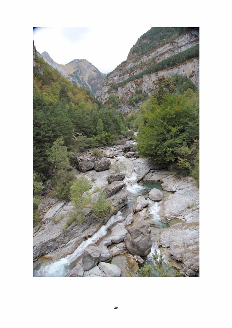
Reserva de la Biosfera Ordesa-Viñamala
La Reserva de la Biosfera de Ordesa-Viñamala fue declarada por la UNESCO en
1977. Su zona núcleo la compone el Parque Nacional de Ordesa y Monte Perdido, el
segundo Parque Nacional más antiguo de España, declarado en 1918. La Reserva
comprende una extensión de 51 396 hectáreas, con un rango altitudinal que va desde los
3555 m hasta los 800 m. Es una de las mejores representaciones de ecosistemas
pirenaicos de montaña y distingue entre dos sectores bien diferenciados: el occidental y
el oriental (Ruiz & Bono, 2001).
El sector occidental está constituido por la Alta Cuenca del Rio Gállego, cuya
naciente está a 2200 m y su punto más bajo dentro de la reserva se sitúa 26 km aguas
abajo, a la altura del pueblo de Biescas, a 840 m. El Gállego es el principal río de la
cuenca y tiene un caudal medio anual de 28,1 m3/s. Su cuenca de drenaje abarca una
superficie de 300 km2 y constituye la zona de transición de la Reserva de la Biosfera. En
su territorio habitan de forma permanente 4000 personas, aunque al tratarse de una zona
con alta actividad turística (pistas de esquí, balnearios, abundante infraestructura
hotelera y campings) la presión poblacional llega a doblarse en épocas de mayor
afluencia turística (verano e invierno). La cuenca presenta también tres grandes
embalses, que sumados a la notable presencia humana ejercen un notable impacto sobre
los ecosistemas fluviales.
El sector oriental está constituido por la cuenca del río Ara, cuya naciente se
sitúa a 2930 m y el punto en el que abandona el territorio de la reserva está a 860 m, en
el municipio de Broto. El río Ara tiene un recorrido de 26 km dentro de la reserva, una
cuenca de 350 km2 y un caudal medio anual de 18.2 m3/s. Todo el territorio de su
cuenca está situado dentro de la zona buffer (o amortiguación) de la reserva, colindante
43
con la zona núcleo, el Parque Nacional de Ordesa y Monte Perdido. En total habitan
unas 900 personas en la zona, y aunque también cuenta con infraestructura turística, la
presión ejercida es significativamente menor que para la cuenca del Alto Gállego, por lo
que los impactos antrópicos son notablemente menores. Además, el río Ara es el último
río libre del Pirineo, el único que todavía no ha sido represado.
Este contexto territorial con dos sistemas hidrográficos paralelos, con
características ambientales e geomorfológicas muy similares, pero expuestos a dos
realidades muy diferentes representa un interesante caso de estudio. Una cuenca
hidrográfica con una protección ambiental más estricta (zona buffer de la reserva) y
menos alterada, frente a otra con una protección mucho más laxa (zona de transición) y
mucho más impactada. El escenario es ideal para poner a prueba la efectividad de
nuestra metodología de muestreo, para llevar a cabo un diagnóstico ambiental y
comparar los resultados de estas dos realidades de gestión ambiental sobre los
ecosistemas fluviales. Así, este trabajo sirve de referencia a la hora de analizar el
pasado, presente y futuro de las otras cuencas fluviales estudiadas, que, aunque
diferentes biogeográficamente, se enfrentan a las mismas amenazas con perspectivas de
futuro similares.
Los ríos de los Andes Tropicales Río Hacha – Colombia
El río Hacha está situado al sur de Colombia, en el piedemonte Andino-
Amazónico de la cordillera oriental. Comprende una cuenca de 490 km2 con un caudal
medio anual de 35.7 m3/s, y fluye a lo largo de 65 km en un rango altitudinal que va
desde su naciente a 2575 m hasta los 240 m en su confluencia con el río Orteguaza. Sus
aguas drenan al río Caquetá, el principal afluente del Amazonas en Colombia. El
territorio de la cuenca está habitado por unos 167 000 habitantes, concentrados la
mayoría en la ciudad de Florencia.
La mayoría de la cuenca (un 89%) pertenece al piedemonte de los Andes, con
fuertes pendientes (media de 7,3%), valles estrechos en forma de V, con fuertes
corrientes y cauces casi lineares y muy erosivos. A partir de los 300 m, la pendiente
empieza a disminuir hasta el 0.06%, al entrar en llanura Amazónica. Es aquí donde se
sitúa la ciudad de Florencia. A partir de este punto el río se ancha, la velocidad del agua
44
disminuye y se forma un cauce meándrico que constituye un extenso valle aluvial. Las
cabeceras boscosas (por encima de los 1000 m) están muy bien conservadas y
protegidas dentro de la Zona de Reserva Forestal de la Amazonia Colombiana desde
1959. La ganadería es la principal actividad y ocupa un 19,9% del territorio. La
agricultura es de subsistencia y apenas cubre un 1.8% del área de la cuenca.
Río Suaza – Colombia
El río Suaza nace dentro del Parque Nacional Natural Cueva de los Guácharos,
primer parque nacional declarado en Colombia en 1960, y pertenece a la Reserva de la
Biosfera Cinturón Andino, nombrada por la UNESCO en 1979. Se ubica al sur de la
cordillera oriental de los Andes Colombianos y es la cuenca hidrográfica colindante al
río Hacha. Sin embargo, está situada al otro lado de la divisoria de aguas, por lo que en
lugar de pertenecer a la cuenca Amazónica forma parte del sistema hidrográfico del río
Magdalena, cuyas aguas fluyen al mar Caribe.
La porción de cuenca estudiada fluye a lo largo de unos 70 km, desde su
naciente a 2840 m, hasta las inmediaciones del municipio de Suaza, a uno 900 m, y
abarca una superficie de unos 660 km2 . Su caudal medio anual es de unos 41,2 m3/s. La
parte alta de la cuenca, situada dentro del parque nacional y siendo también la zona
núcleo y buffer de la reserva de la biosfera, está totalmente cubierta de bosque primario
y la forman estrechos y empinados valles en forma de “v”. A los 1280 m, ya fuera de
los límites de la Reserva de la Biosfera, la pendiente disminuye, el valle se abre y
aparecen los primeros asentamientos humanos. La mayoría de la cuenca a partir de ese
punto está deforestada (en un 75%) y predominan grandes superficies de pasto para usos
ganaderos. La población total de la zona suma unas 52 000 personas, y aunque existen
dos núcleos urbanos situados a las orillas del río Suaza (Suaza y Acevedo), casi el 80%
de los habitantes están dispersos en pequeños asentamientos rurales.
Río Alto Madre de Dios – Perú
La cuenca del Alto Madre de Dios está situada en el piedemonte Andino-
Amazónico de Perú, al suroeste del país. Conforma la zona de transición de la Reserva
de la Biosfera del Manu, declarada por la UNESCO en 1977, siendo el Parque Nacional
de Manu (establecido en 1973) su zona núcleo. El territorio estudiado abarca una cuenca
45
de 410 km2 por la cual el río Alto Madre de Dios fluye a lo largo de 80 km desde una
altitud de 3500 m hasta los 300 m. Hasta los 700 m de altura la cuenca está formada por
estrechos valles montañosos que discurren por las pendientes de los Andes, totalmente
cubiertas de bosque primario, para dar paso después a territorios de llanura, con valles
aluviales más abiertos. Es aquí donde aparecen los asentamientos humanos, con el
pueblo de Pilcopata como núcleo principal, y que suman un total de 4790 habitantes.
Una vez la cuenca abandona las estribaciones de los Andes es cuando empiezan a
aparecer cambios en los usos del territorio, con zonas deforestadas por la explotación
maderera y parte del territorio dedicada a explotaciones ganaderas extensivas.
Características comunes de las cuencas estudiadas
Aunque aparentemente muy diferentes, las cinco cuencas estudiadas comparten
unas características que las hacen comparables y hacen replicable la metodología de
muestreo seleccionada. Todos los ecosistemas fluviales estudiados son ríos de montaña
(Pirenaicos y Andinos). Aunque su rango altitudinal sea muy amplio (desde los 3500 m
de el Alto Madre de Dios, hasta los 250 m del río Hacha), todos ellos presentan un
patrón hidromorfológico similar y muestran un solapamiento de patrones ambientales y
antrópicos.
La mayoría del territorio de todas las cuencas estudiadas corresponde a ríos de
montaña: pronunciadas pendientes; valles estrechos y encajados en forma de “v”;
fuertes corrientes; cauces erosivos; sustratos de gran tamaño; aguas oligotróficas, frías,
con bajas conductividades y muy oxigenadas; cuencas poco alteradas y cubiertas de
bosque primario; organismos fuertemente adaptados. Y en todos los casos, en el punto
en el que la geomorfología cambia y las pendientes montañosas dan paso a zonas más
llanas, el territorio y los ecosistemas fluviales presentan características comunes: valles
abiertos más abiertos con llanuras de inundación; cauces anastomosados; corrientes más
lentas; procesos de sedimentación; sustratos finos; aguas mesotróficas, más calientes,
menos oxigenadas, con conductividades más altas; presencia de asentamientos humanos
y presiones antrópicas; sin protección ambiental (o con protección laxa); territorios de la
cuenca alterados; cambio a usos del suelo productivos (ganadería extensiva y
agricultura).
46
Presentación de los capítulos
A continuación se presentan brevemente los trabajos resultantes de esta tesis
doctoral y se explica el orden y formato elegidos para su exposición:
El primer capítulo incluye el análisis y comparación de las cuencas pirenaicas de
los ríos Gállego y Ara. Los otros seis capítulos presentan los casos estudiados en los
Andes Tropicales. Aunque separados por cuestiones relacionadas con objetivos de
publicación, deben ser considerados como tres bloques. El primer capítulo de cada
bloque expone de forma detallada el estudio ecológico y diagnóstico para las cuencas
del río Hacha (Capítulo 2), río Suaza (Capítulo 4) y río Alto Madre de Dios (Capítulo
6). Complementarios a cada uno de estos trabajos, los capítulos restantes son notas
técnicas con los resultados de las relaciones longitud-peso de las especies de peces más
abundantes para la cuenca del río Hacha (Capítulo 3), río Suaza (Capítulo 5) y río Alto
Madre de Dios (Capítulo 7).

47
48
49
CAPÍTULO 1ST CHAPTER DIAGNOSTICANDO LA INTEGRIDAD DEL ECOSISTEMA FLUVIAL EN LA RESERVA DE LA BIOSFERA ORDESA‐VIÑAMALA Diagnosing stream ecosystem integrity in the Ordesa‐Viñamala Biosphere Reserve
Tobes I, Gaspar S, Oscoz J, Miranda R
Journal of Applied Ichthyology, 32 (1): 229‐239 (2016)

50
51
Resumen
Este trabajo estudia la integridad ecológica de los ecosistemas fluviales dentro de la Reserva
de la Biosfera Ordesa-Viñamala. A pesar de su estado de protección, la Reserva de la Biosfera
Ordesa-Viñamala sufre una considerable presión antrópica. El presente trabajo aspira a
evaluar y comparar el estado de conservación de las dos cuencas que se encuentran dentro del
área protegida. La cuenca del río Gállego, situada dentro del área de transición de la Reserva
de la Biosfera, permite un amplio rango de actividades humanas. De forma paralela, la cuenca
del Ara, está situada dentro del área de amortiguamiento, donde sólo se permiten prácticas
ecológicamente respetuosas. El estado medioambiental de los ecosistemas fluviales fue
analizado estudiando las comunidades de peces y macroinvertebrados, las características del
hábitat, las variables físico-químicas y calculando varios índices de calidad ambiental. Desde
agosto a septiembre de 2011 se muestrearon un total de 14 lugares. Los muestreos de peces se
realizaron usando un equipo de pesca eléctrica y los macroinvertebrados se muestrearon
aplicando los procedimientos IBMWP y IASPT. Nuestros resultados mostraron que, mientras el
río Ara mantiene una buena integridad ecológica, el río Gállego muestra importantes
alteraciones del hábitat. La trucha, la especie dominante y exclusiva del río Ara, estaba ausente
y reemplazada por ciprínidos nativos translocados en algunos puntos del río Gállego. Esta
colonización se explicó por la alteración de los ecosistemas fluviales y su homogeneización. El
estudio de las comunidades de macroinvertebrados y la diagnosis obtenida con los índices de
calidad ambiental también mostró la deficiente integridad ecológica de algunos lugares en el
río Gállego. Nuestros resultados sugieren que la figura de la Reserva de la Biosfera no está
proporcionando una protección adecuada a los ríos dentro de sus límites, que conducen a una
degradación importante de su integridad biológica.
Palabras clave: peces endémicos, calidad medioambiental, índices bióticos, evaluación del
estado ecológico.
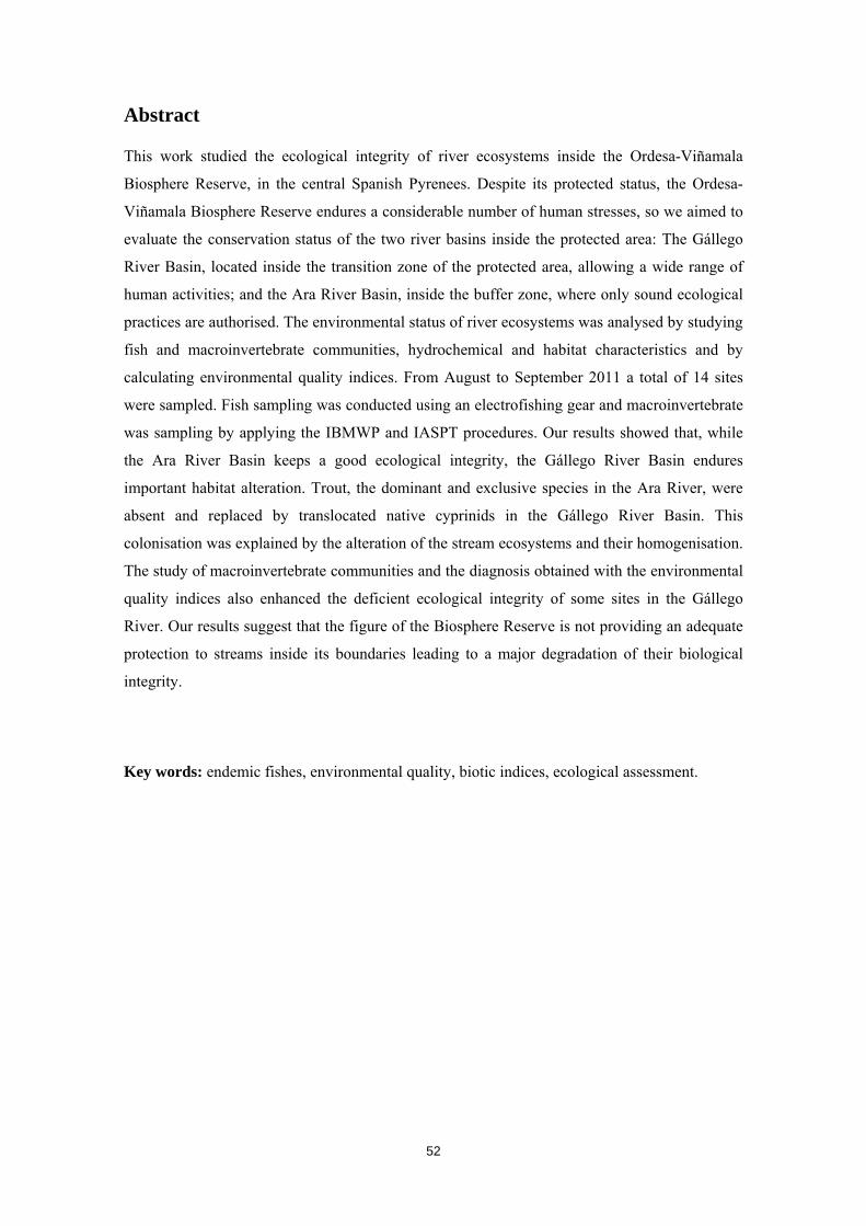
52
Abstract
This work studied the ecological integrity of river ecosystems inside the Ordesa-Viñamala
Biosphere Reserve, in the central Spanish Pyrenees. Despite its protected status, the Ordesa-
Viñamala Biosphere Reserve endures a considerable number of human stresses, so we aimed to
evaluate the conservation status of the two river basins inside the protected area: The Gállego
River Basin, located inside the transition zone of the protected area, allowing a wide range of
human activities; and the Ara River Basin, inside the buffer zone, where only sound ecological
practices are authorised. The environmental status of river ecosystems was analysed by studying
fish and macroinvertebrate communities, hydrochemical and habitat characteristics and by
calculating environmental quality indices. From August to September 2011 a total of 14 sites
were sampled. Fish sampling was conducted using an electrofishing gear and macroinvertebrate
was sampling by applying the IBMWP and IASPT procedures. Our results showed that, while
the Ara River Basin keeps a good ecological integrity, the Gállego River Basin endures
important habitat alteration. Trout, the dominant and exclusive species in the Ara River, were
absent and replaced by translocated native cyprinids in the Gállego River Basin. This
colonisation was explained by the alteration of the stream ecosystems and their homogenisation.
The study of macroinvertebrate communities and the diagnosis obtained with the environmental
quality indices also enhanced the deficient ecological integrity of some sites in the Gállego
River. Our results suggest that the figure of the Biosphere Reserve is not providing an adequate
protection to streams inside its boundaries leading to a major degradation of their biological
integrity.
Key words: endemic fishes, environmental quality, biotic indices, ecological assessment.
53
Introduction
Protected areas are a mainstay of biodiversity conservation throughout the world
(Gaston et al., 2008; Chessman, 2013), but uncertainty relative to their effectiveness is
particularly high in the cases were biodiversity indicators are used in freshwaters
(Herbert et al., 2010). Protected status per se may not adequately conserve freshwater
biodiversity especially where the principal threats are habitat destruction and
interferences caused by arriving alien species (Maceda-Veiga, 2012).
Biosphere Reserves (BR) are internationally recognized protected areas within
the framework of the “UNESCO Programme on Man and the Biosphere (MaB)”
(UNESCO, 1996) created for reconciling conservation and sustainable use of the
resources. They comprise three different protection zones: (a) core area, securely
protected; (b) buffer zones, allowing low-impact activities; (c) transition areas, used for
managing and developing resources that can be utilized by man in a sustainable manner.
At a time when the region is facing increasing development pressures it is
necessary to detect existing environmental issues, make steps forward for solving them
and prevent future threats. As rivers integrate all that happens in their landscapes, their
biological condition tells much about the side effects of human actions detecting the
causes and consequences of change, especially those that alter living systems (Karr,
1998). Therefore streams and biological communities are sensitive indicators of the
relative health of the aquatic ecosystems and their surrounding catchment (Fausch et al.,
2002; Hering et al., 2006).
The aims of this paper were 1) to carry out an integral evaluation of the
environmental status of freshwater systems inside the Ordesa-Viñamala BR, in the
central Spanish Pyrenees, emphasizing the fish communities 2) to detect environmental
impacts and to study their origin, processes and consequences, and 3) to evaluate the
effectiveness of the protected area for the conservation of the river ecosystems within
the reserve.
54
Materials and methods
Study area
The Ordesa-Viñamala BR is located within the central Spanish Pyrenees with
the headwater area of the Gállego and the Ara River systems (Fig. 1). Both rivers
belong to the Ebro River Basin and flow in parallel through two adjacent valleys.
Figure 1. Location of study sites in the Ara and Gállego River Basins, in the Ordesa-Viñamala Biosphere Reserve. Dark-dotted areas represent urban surfaces. The coding of samples sites is used in all figures and tables.
The climate in the area is quite heterogeneous due to the extreme
geomorphology and ranges from mountainous territories with oceanic influence,
rainfalls totalling 2000 mm year-1 and a mean annual temperature of 5ºC, to dryer
mountainous areas with a marked continentality. The Reserve is dominated by mixed
mountain and highland systems, with extensive areas of rocky habitats. Forested areas
have mixed woodlands of beech (Fagus sylvatica L.) and conifers such as Pinus
sylvestris L. Higher reaches are occupied by black mountain pine (Pinus uncinata Ram.
ex A.DC.) and widespread pasturelands (Pérez and Alonso, 1994).
The upper Gállego River (drainage area 300 km2) runs 26 km from its source at
2200 meters above sea level (m a.s.l.) to the village of Biescas (840 m a.s.l.), and
encompasses three tributaries, the Aguas Limpias (G01), Caldares (G04) and Bolatica
55
Rivers (G05). Three reservoirs collect the water of the Gállego River (Fig. 1). A large
skiing area is also within the basin. The average multi-annual water flow downstream
Bubal Reservoir is 28.1 m3 s-1. Several towns are in the area (about 4000 inhabitants).
The Gállego River draws the western boundary of the BR, and only the eastern side of
its basin is located inside the reserve, in the transition zone.
The headwater area of the Ara River Basin is the contiguous watershed (Fig. 1)
covering about 350 km2 and runs 26 km from its source at 2 930 m a.s.l. to the village
of Broto at 867 m a.s.l. There are few towns in the area (about 900 inhabitants). The Ara
River is the last “free running” river in the Pyrenees, without any dams. The average
multi-annual water flow is 18.2 m3 s-1. The watershed is located in the core and the
buffer area of the BR.
Data collection
From August to September 2011 a total of 14 sites were sampled along the
Gállego River Basin (five sites for the Gállego River and three sites for its tributaries)
and the Ara River (six sites) (Fig. 1).
At each sampling site, temperature (precision 0.1 °C), dissolved oxygen
(precision 0.01 mg l-1), pH, and electrical conductivity (precision 1 µS cm-1) were
measured with a multi-parameter water quality monitoring system (WTW Multi
340i).The instruments were calibrated daily during sampling period. Besides water
samples were collected. These samples were stored in ice and processed in the
laboratory one day later. Anions were analysed using ion chromatography (Dionex ICS-
2000) and cations were measured using an inductively coupled plasma mass
spectrometry (ICP-MS, Agilent 7500a). The analysed parameters were chloride (Cl-1)
(mg l-1), sulphate (SO42-) (mg l-1), nitrate (NO-2) (mg l-1) and nitrite (NO-3) (mg l-1) as
indicators of trophic status of the area (Table 1) (Pesce and Wunderlin, 2000). Habitat
structures were characterised by factors such as depth (m), water velocity (m s-1), tree
canopy shading percentage and dominant substrate, categorised as fines (<2 mm),
gravels (2-64 mm), cobbles (64-256 mm), boulders (>256 mm) and bedrock (Table 1)
(Armantrout, 1998).
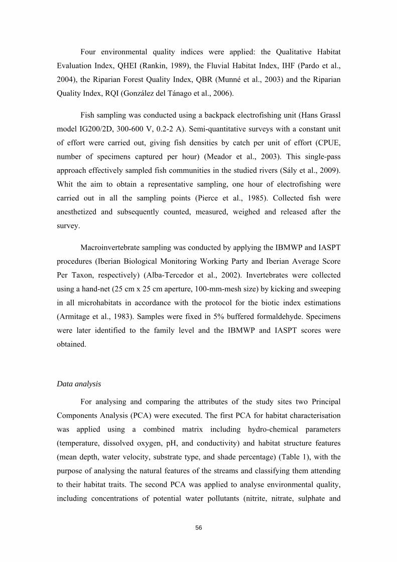
56
Four environmental quality indices were applied: the Qualitative Habitat
Evaluation Index, QHEI (Rankin, 1989), the Fluvial Habitat Index, IHF (Pardo et al.,
2004), the Riparian Forest Quality Index, QBR (Munné et al., 2003) and the Riparian
Quality Index, RQI (González del Tánago et al., 2006).
Fish sampling was conducted using a backpack electrofishing unit (Hans Grassl
model IG200/2D, 300-600 V, 0.2-2 A). Semi-quantitative surveys with a constant unit
of effort were carried out, giving fish densities by catch per unit of effort (CPUE,
number of specimens captured per hour) (Meador et al., 2003). This single-pass
approach effectively sampled fish communities in the studied rivers (Sály et al., 2009).
Whit the aim to obtain a representative sampling, one hour of electrofishing were
carried out in all the sampling points (Pierce et al., 1985). Collected fish were
anesthetized and subsequently counted, measured, weighed and released after the
survey.
Macroinvertebrate sampling was conducted by applying the IBMWP and IASPT
procedures (Iberian Biological Monitoring Working Party and Iberian Average Score
Per Taxon, respectively) (Alba-Tercedor et al., 2002). Invertebrates were collected
using a hand-net (25 cm x 25 cm aperture, 100-mm-mesh size) by kicking and sweeping
in all microhabitats in accordance with the protocol for the biotic index estimations
(Armitage et al., 1983). Samples were fixed in 5% buffered formaldehyde. Specimens
were later identified to the family level and the IBMWP and IASPT scores were
obtained.
Data analysis
For analysing and comparing the attributes of the study sites two Principal
Components Analysis (PCA) were executed. The first PCA for habitat characterisation
was applied using a combined matrix including hydro-chemical parameters
(temperature, dissolved oxygen, pH, and conductivity) and habitat structure features
(mean depth, water velocity, substrate type, and shade percentage) (Table 1), with the
purpose of analysing the natural features of the streams and classifying them attending
to their habitat traits. The second PCA was applied to analyse environmental quality,
including concentrations of potential water pollutants (nitrite, nitrate, sulphate and
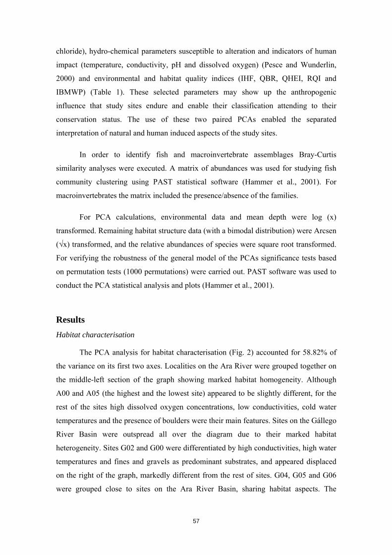
57
chloride), hydro-chemical parameters susceptible to alteration and indicators of human
impact (temperature, conductivity, pH and dissolved oxygen) (Pesce and Wunderlin,
2000) and environmental and habitat quality indices (IHF, QBR, QHEI, RQI and
IBMWP) (Table 1). These selected parameters may show up the anthropogenic
influence that study sites endure and enable their classification attending to their
conservation status. The use of these two paired PCAs enabled the separated
interpretation of natural and human induced aspects of the study sites.
In order to identify fish and macroinvertebrate assemblages Bray-Curtis
similarity analyses were executed. A matrix of abundances was used for studying fish
community clustering using PAST statistical software (Hammer et al., 2001). For
macroinvertebrates the matrix included the presence/absence of the families.
For PCA calculations, environmental data and mean depth were log (x)
transformed. Remaining habitat structure data (with a bimodal distribution) were Arcsen
(√x) transformed, and the relative abundances of species were square root transformed.
For verifying the robustness of the general model of the PCAs significance tests based
on permutation tests (1000 permutations) were carried out. PAST software was used to
conduct the PCA statistical analysis and plots (Hammer et al., 2001).
Results
Habitat characterisation
The PCA analysis for habitat characterisation (Fig. 2) accounted for 58.82% of
the variance on its first two axes. Localities on the Ara River were grouped together on
the middle-left section of the graph showing marked habitat homogeneity. Although
A00 and A05 (the highest and the lowest site) appeared to be slightly different, for the
rest of the sites high dissolved oxygen concentrations, low conductivities, cold water
temperatures and the presence of boulders were their main features. Sites on the Gállego
River Basin were outspread all over the diagram due to their marked habitat
heterogeneity. Sites G02 and G00 were differentiated by high conductivities, high water
temperatures and fines and gravels as predominant substrates, and appeared displaced
on the right of the graph, markedly different from the rest of sites. G04, G05 and G06
were grouped close to sites on the Ara River Basin, sharing habitat aspects. The
58
remaining sites, G01, G03 and G07 formed another cluster on the left bottom area of the
diagram, distinguished by high water velocities and pebbles as dominating substrate.
Figure 2. PCA biplot of study for habitat characterisation: Water physicochemical parameters (temperature, oxygen concentration, pH and conductivity) and physical habitat parameters (substrate type, mean width, mean depth, mean water velocity and shaded percentage of the river channel).
Environmental quality
The PCA biplot for environmental quality accounted on its two first axes for
66.30% of the variance (Fig. 3). The first axis explained 42.69% of the variability,
separating sites with good environmental quality on the left, influenced by high values
of the environmental quality indices, opposed to high concentrations of water nutrients.
All the sites on the Ara River except A05 were located on this area of the plot among
sites G01, G04, G05 and G06 showing good ecological integrity. Site G02 appeared
notoriously displaced on the right upper area of the plot, showing the highest
anthropogenic alteration.
The second axis accounted for the remaining 23.61% of variability and
discriminated sites showing greater physical habitat degradation but with lesser water
59
pollution, distributing them on the right bottom area of the graph. The lowest sites on
both basins, A05 and G07 were grouped here suffering similar alteration due to the
presence of urban areas, canalisation and sewage. Site G03, on the central bottom area
of the plot, presented low concentrations of water pollutants but important physical
habitat degradation, explained by the almost artificial morphology of the river channel
that flows excavating the tail sediments area of the Bubal Reservoir. Finally, site G00
appeared on the right bottom area of the graph, presenting remarkable water and habitat
alterations.
Figure 3. PCA biplot of study sites for ecological integrity: Environmental quality indices (QHEI, QBR, RQI, IHF and IBMWP), nutrients (nitrite, nitrate, chloride and sulphate concentration) and hydrochemical parameters (temperature, oxygen concentration, pH and conductivity).
Fish and macroinvertebrate species composition
A total of 1,978 specimens (four species of two families) was collected (Table
2). All species were native: one autochthonous salmonid (brown trout Salmo trutta
Linnaeus 1758) and three endemic cyprinids (Ebro nase Parachondrostoma miegii
Steindachner 1866, Pyrenean gudgeon Gobio lozanoi Doadrio & Madeira 2004 and
Pyrenean minnows Phoxinus bigerri Kottelat 2007). The cluster analysis for fish
separated sites in three groups (Fig. 4). The majority of them were grouped together
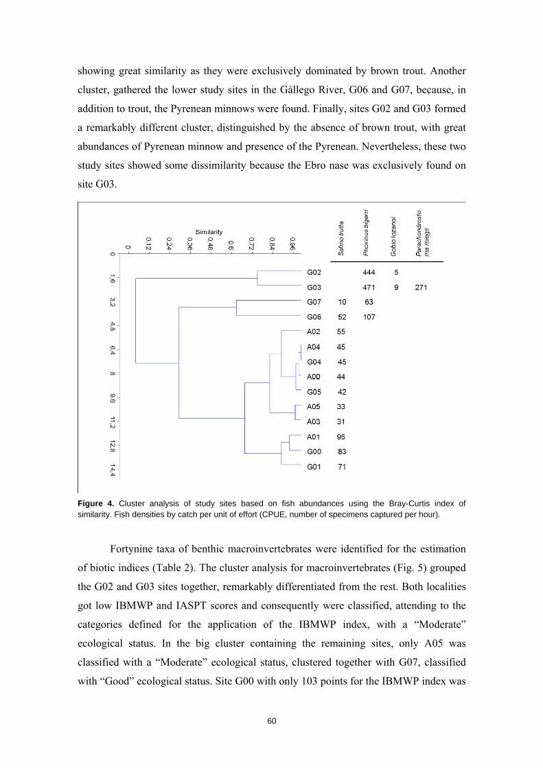
60
showing great similarity as they were exclusively dominated by brown trout. Another
cluster, gathered the lower study sites in the Gállego River, G06 and G07, because, in
addition to trout, the Pyrenean minnows were found. Finally, sites G02 and G03 formed
a remarkably different cluster, distinguished by the absence of brown trout, with great
abundances of Pyrenean minnow and presence of the Pyrenean. Nevertheless, these two
study sites showed some dissimilarity because the Ebro nase was exclusively found on
site G03.
Figure 4. Cluster analysis of study sites based on fish abundances using the Bray-Curtis index of similarity. Fish densities by catch per unit of effort (CPUE, number of specimens captured per hour).
Fortynine taxa of benthic macroinvertebrates were identified for the estimation
of biotic indices (Table 2). The cluster analysis for macroinvertebrates (Fig. 5) grouped
the G02 and G03 sites together, remarkably differentiated from the rest. Both localities
got low IBMWP and IASPT scores and consequently were classified, attending to the
categories defined for the application of the IBMWP index, with a “Moderate”
ecological status. In the big cluster containing the remaining sites, only A05 was
classified with a “Moderate” ecological status, clustered together with G07, classified
with “Good” ecological status. Site G00 with only 103 points for the IBMWP index was
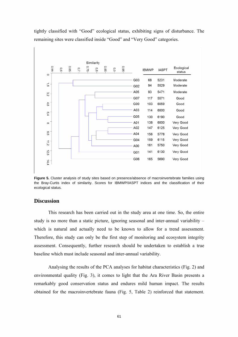
61
tightly classified with “Good” ecological status, exhibiting signs of disturbance. The
remaining sites were classified inside “Good” and “Very Good” categories.
Figure 5. Cluster analysis of study sites based on presence/absence of macroinvertebrate families using the Bray-Curtis index of similarity. Scores for IBMWP/IASPT indices and the classification of their ecological status.
Discussion
This research has been carried out in the study area at one time. So, the entire
study is no more than a static picture, ignoring seasonal and inter-annual variability –
which is natural and actually need to be known to allow for a trend assessment.
Therefore, this study can only be the first step of monitoring and ecosystem integrity
assessment. Consequently, further research should be undertaken to establish a true
baseline which must include seasonal and inter-annual variability.
Analysing the results of the PCA analyses for habitat characteristics (Fig. 2) and
environmental quality (Fig. 3), it comes to light that the Ara River Basin presents a
remarkably good conservation status and endures mild human impact. The results
obtained for the macroinvertebrate fauna (Fig. 5, Table 2) reinforced that statement.

62
Concerning fish fauna, streams were exclusively dominated by brown trout (Fig. 4) as
expected for this sort of rivers.
On the other hand, the results obtained for the Gállego River Basin highlighted a
remarkable human impact. The PCA analysis for environmental quality brought out the
degraded sites that combined with the PCA for habitat characterisation and cluster
analyses for macroinvertebrates and fish helped identify the most damaged river
stretches.
Site G00 was identified as an altered locality by both PCA analyses, although it
was not stressed as impacted by the invertebrate and fish analyses. The fish community
was exclusively composed by brown trout, showing one of the most abundant
populations (Table 2). The majority of the trout individuals were fry with +0 or +1 age.
That fact, along with the features of the habitat, distinguished by the abundance of
gravels and shallow waters, pointed out the site as a trout spawning area (Shirvell and
Dungey, 1983). Comparing it with the G01 site in the Aguas Limpias River (another
trout spawning area found in the adjacent valley at same elevation and sharing similar
natural features) or even with A01 (also an analogous locality in the Ara River), the
difference between them was notorious. While G01 and A01 localities demonstrated a
remarkable high environmental quality for the river and for the surrounding landscape,
G00 showed several traces of habitat degradation. The PCA for habitat characterisation
(Fig. 2) addressed the outstanding high water temperatures, the lack of shade and the
presence of fine substrates, while the environmental quality PCA analysis also
addressed the physical habitat and water quality degradation. This river stretch is totally
isolated from the rest of the basin due the presence downstream of the Gállego
Reservoir. In addition to the impact of the dam, urban areas, sewage and ripraps affect
its ecological integrity. However the greatest menaces upon this river stretch are the
increase of water temperature due to the total exposure of the river channel lacking
riparian vegetation and the remarkable siltation process caused by major soil erosion, as
a consequence of the extensive deforestation of the hillsides occupied by the Formigal
ski slopes (David et al., 2009). Both impacts, accentuated by the presence of physical
barriers that impede migration, can lead to the siltation and disappearance of suitable
spawning areas (Acornley and Sear, 1999) and together with the thermal habitat
alteration (Elliott, 1976) finally can cause the extinction of trout populations in this area.
63
The faunal composition of streams is thought to reflect ambient conditions and
integrate the influences of water quality and habitat degradation (Allan, 2004).
Therefore the unexpected reophilic cyprinids communities on G02 and G03 sites
pointed out an outstanding change in the river ecosystem (García de Jalón, 1996). The
abundance of these fish out of their expected distribution range could be considered as a
native fish invasion (Scott and Helfman, 2001; Leunda, 2010) and an indicator of the
habitat alteration (Courtenay and Moyle, 1996).
The process of invasion necessarily involves habitat destruction (Moyle and
Leidy, 1992) prior to human introduction of those new fish species, usually by the hand
of anglers utilising them as bait or forage (Maceda-Veiga et al., 2010). Unique and
limiting elements like the flood occurrence and clean cold waters are displaced and
eventually replaced by common, widespread elements (Scott and Helfman, 2001).
Water temperatures and sediment loads increase due to the lack of riparian vegetation
(Acuña et al.. 2013), flood occurrence disappears controlled by dams (García de Jalón et
al., 1988), reservoirs provide suitable lentic habitats (Clavero et al. 2004) resulting in
invasions of the streams that flow into them (García de Jalón, 1996) and nutrient
enrichment enhances phytobenthic biomass and favours phytophagous omnivorous
species like the Ebro nase (Maceda-Veiga, 2012). In consequence, highland stream
conditions change sufficiently to facilitate the establishment of widespread native fish
like the Ebro nase and the Pyrenean Minnow (Jones et al., 1999). At the same time,
these new habitat conditions may turn out to be adverse for upland endemics like the
trout (Elliot, 1976) and the presence of new fish species like the Pyrenean minnow, that
may result in trophic competition for resources at the larval and juvenile stages (Oscoz
et al., 2008), could end up with the disappearance of trout from these streams.
The replacement of trout from these headwater streams is usually overlooked
because these native invasions first lead to no change in diversity and perhaps even an
increase in diversity (Courtenay and Moyle 1996), a fact that has been found in a variety
of aquatic systems subject to invasions (Rahel, 2000). As stated by Pusey et al. (2006)
there is no reason to believe that the consequences derived from the introduction of non-
native indigenous species would be any different to those arising from the introduction
of fishes from other countries (del Carpio et al., 2010). This is the case of the studied
streams, being the Ebro nase, the Pyrenean minnow and the Pyrenean gudgeon the
64
translocated fish species (Leunda, 2010). Therefore, such invasions should be
recognized as an early warning sign of the homogenization process of the river
ecosystem (Scott and Helfman, 2001) and considered as a wake-up-call of major
environmental alteration.
The early detection of environmental threats is becoming essential for
developing efficient strategies and to prevent major and irreversible alterations (Allan,
2004). The present work proved the reliability of the study of the ecological integrity of
the streams for detecting impacts in the surrounding landscape (Karr, 1998). Even for
idyllic sceneries like the central Pyrenees, where everything looks pristine and
uncorrupted, rivers, as impact collectors, highlight the anthropogenic pressure endured
by the territory.
The studied area possesses a remarkable number of protected zones with a wide
range of protection levels (National Park designed by the Spanish Government and
Biosphere Reserve by UNESCO, among others). There is no doubt about the
effectiveness of the designation of a National Park and core area of a BR, but
concerning the protection given by the buffer and transition zones, it was remarkable the
different ecological integrity shown by the sites located on the buffer zone and the ones
on the transition zone. As seen before, the Ara River Basin located mostly inside the
buffer zone demonstrated a very good conservation status. In contrast, the Gállego River
Basin located on the transition zone, with the Gállego River drawing the limits of the
reserve, presented a remarkable alteration at some localities. This is due to the wider
range of land uses that the transition area endures and because only the left margin of
the basin is found inside the reserve, leaving the right margin unprotected. Terrestrial
protected areas often include only part of a river’s catchment or use rivers as boundaries
rather than fully including them (Nel et al., 2007). Consequently, rivers within protected
areas are often vulnerable to transmission of impacts from land and water use beyond
their boundaries (Pringle 2001). Furthermore, some stretches of the Gállego River are
not even included inside the BR, even as a boundary. These areas were excluded from
the designation of the territories inside the reserve because they were already urbanized
or occupied by reservoirs. This fact enhances the inconsideration of the Gállego River
as complex, interdependent and unitary ecosystem worthy of being protection target,
demoting it to merely drawing the limits of the protected area. Therefore, if we aspire to
65
effectively preserve these freshwater ecosystems, we should respect their entireness, we
should take into account all the ecological processes involved in their configuration, we
should reckon their tight interconnection with the territories of their watershed and we
should develop specific conservation efforts for guaranteeing their safeguard.
Acknowledgments
This study was sponsored by the Environmental Biology Department of the
Universidad de Navarra, providing logistic and economic resources to complete the
work. We are grateful to I. Azcona, M. E. Elizalde, A. Zapata, I. Vedia, E. Cinto, I.
Salvo, L. Capdet and K. Westfall who assisted carrying out the fieldwork and data
collection.
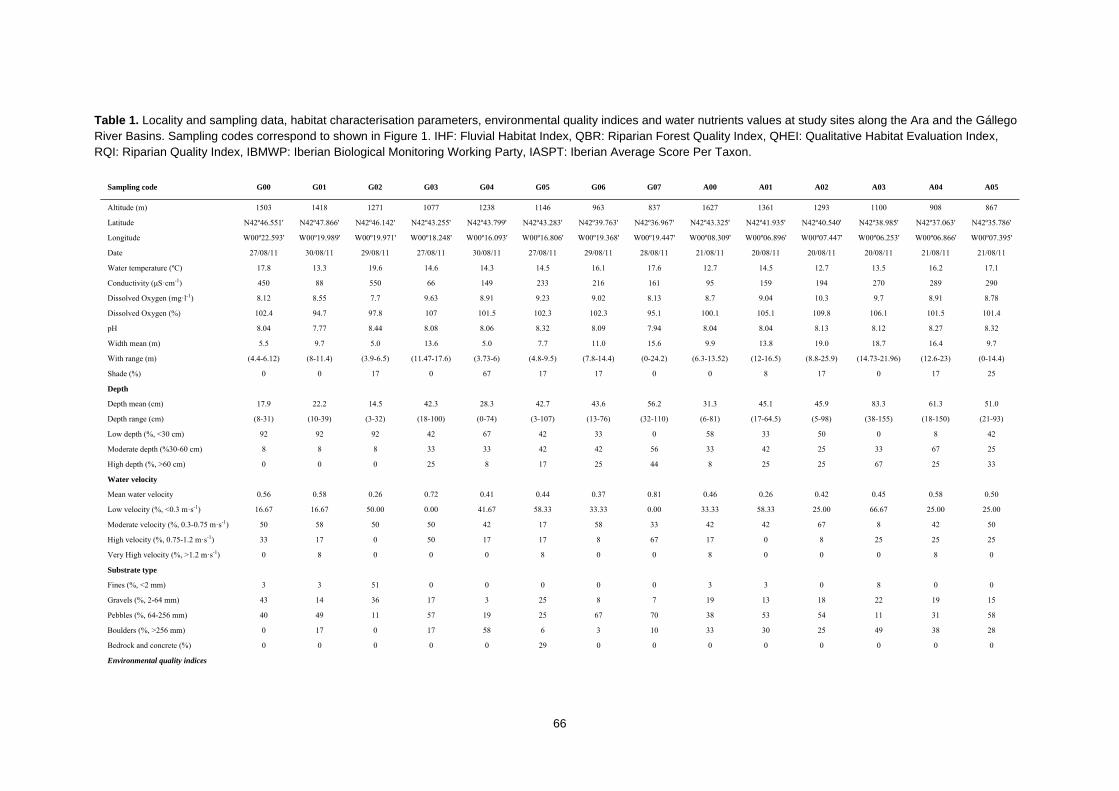
66
Table 1. Locality and sampling data, habitat characterisation parameters, environmental quality indices and water nutrients values at study sites along the Ara and the Gállego River Basins. Sampling codes correspond to shown in Figure 1. IHF: Fluvial Habitat Index, QBR: Riparian Forest Quality Index, QHEI: Qualitative Habitat Evaluation Index, RQI: Riparian Quality Index, IBMWP: Iberian Biological Monitoring Working Party, IASPT: Iberian Average Score Per Taxon.
Sampling code G00 G01 G02 G03 G04 G05 G06 G07 A00 A01 A02 A03 A04 A05
Altitude (m) 1503 1418 1271 1077 1238 1146 963 837 1627 1361 1293 1100 908 867
Latitude N42º46.551' N42º47.866' N42º46.142' N42º43.255' N42º43.799' N42º43.283' N42º39.763' N42º36.967' N42º43.325' N42º41.935' N42º40.540' N42º38.985' N42º37.063' N42º35.786'
Longitude W00º22.593' W00º19.989' W00º19.971' W00º18.248' W00º16.093' W00º16.806' W00º19.368' W00º19.447' W00º08.309' W00º06.896' W00º07.447' W00º06.253' W00º06.866' W00º07.395'
Date 27/08/11 30/08/11 29/08/11 27/08/11 30/08/11 27/08/11 29/08/11 28/08/11 21/08/11 20/08/11 20/08/11 20/08/11 21/08/11 21/08/11
Water temperature (ºC) 17.8 13.3 19.6 14.6 14.3 14.5 16.1 17.6 12.7 14.5 12.7 13.5 16.2 17.1
Conductivity (μS·cm-1) 450 88 550 66 149 233 216 161 95 159 194 270 289 290
Dissolved Oxygen (mg·l-1) 8.12 8.55 7.7 9.63 8.91 9.23 9.02 8.13 8.7 9.04 10.3 9.7 8.91 8.78
Dissolved Oxygen (%) 102.4 94.7 97.8 107 101.5 102.3 102.3 95.1 100.1 105.1 109.8 106.1 101.5 101.4
pH 8.04 7.77 8.44 8.08 8.06 8.32 8.09 7.94 8.04 8.04 8.13 8.12 8.27 8.32
Width mean (m) 5.5 9.7 5.0 13.6 5.0 7.7 11.0 15.6 9.9 13.8 19.0 18.7 16.4 9.7
With range (m) (4.4-6.12) (8-11.4) (3.9-6.5) (11.47-17.6) (3.73-6) (4.8-9.5) (7.8-14.4) (0-24.2) (6.3-13.52) (12-16.5) (8.8-25.9) (14.73-21.96) (12.6-23) (0-14.4)
Shade (%) 0 0 17 0 67 17 17 0 0 8 17 0 17 25
Depth
Depth mean (cm) 17.9 22.2 14.5 42.3 28.3 42.7 43.6 56.2 31.3 45.1 45.9 83.3 61.3 51.0
Depth range (cm) (8-31) (10-39) (3-32) (18-100) (0-74) (3-107) (13-76) (32-110) (6-81) (17-64.5) (5-98) (38-155) (18-150) (21-93)
Low depth (%, <30 cm) 92 92 92 42 67 42 33 0 58 33 50 0 8 42
Moderate depth (%30-60 cm) 8 8 8 33 33 42 42 56 33 42 25 33 67 25
High depth (%, >60 cm) 0 0 0 25 8 17 25 44 8 25 25 67 25 33
Water velocity
Mean water velocity 0.56 0.58 0.26 0.72 0.41 0.44 0.37 0.81 0.46 0.26 0.42 0.45 0.58 0.50
Low velocity (%, <0.3 m·s-1) 16.67 16.67 50.00 0.00 41.67 58.33 33.33 0.00 33.33 58.33 25.00 66.67 25.00 25.00
Moderate velocity (%, 0.3-0.75 m·s-1) 50 58 50 50 42 17 58 33 42 42 67 8 42 50
High velocity (%, 0.75-1.2 m·s-1) 33 17 0 50 17 17 8 67 17 0 8 25 25 25
Very High velocity (%, >1.2 m·s-1) 0 8 0 0 0 8 0 0 8 0 0 0 8 0
Substrate type
Fines (%, <2 mm) 3 3 51 0 0 0 0 0 3 3 0 8 0 0
Gravels (%, 2-64 mm) 43 14 36 17 3 25 8 7 19 13 18 22 19 15
Pebbles (%, 64-256 mm) 40 49 11 57 19 25 67 70 38 53 54 11 31 58
Boulders (%, >256 mm) 0 17 0 17 58 6 3 10 33 30 25 49 38 28
Bedrock and concrete (%) 0 0 0 0 0 29 0 0 0 0 0 0 0 0
Environmental quality indices
67
IHF 63 64 63 59 78 69 76 60 62 67 64 66 60 58
QBR 5 90 40 30 100 40 90 30 60 60 90 95 90 65
QHEI 48 68 58 53.5 84 63 75 61.5 69.5 65.5 74 80 76.5 62
RQI 18 87 62 33 94 62 82 52 46 51 71 97 95 72
IBMWP 103 141 94 68 159 130 165 117 161 138 147 114 156 93
IASPT 6059 6130 5529 5231 6115 6190 5690 5571 5750 6000 6125 6000 5778 5471
Stream class II I III I I II I II I I I II I II
Ecological status Good Very good Moderate Moderate Very good Good Very good Good Very good Very good Very good Good Very good Moderate
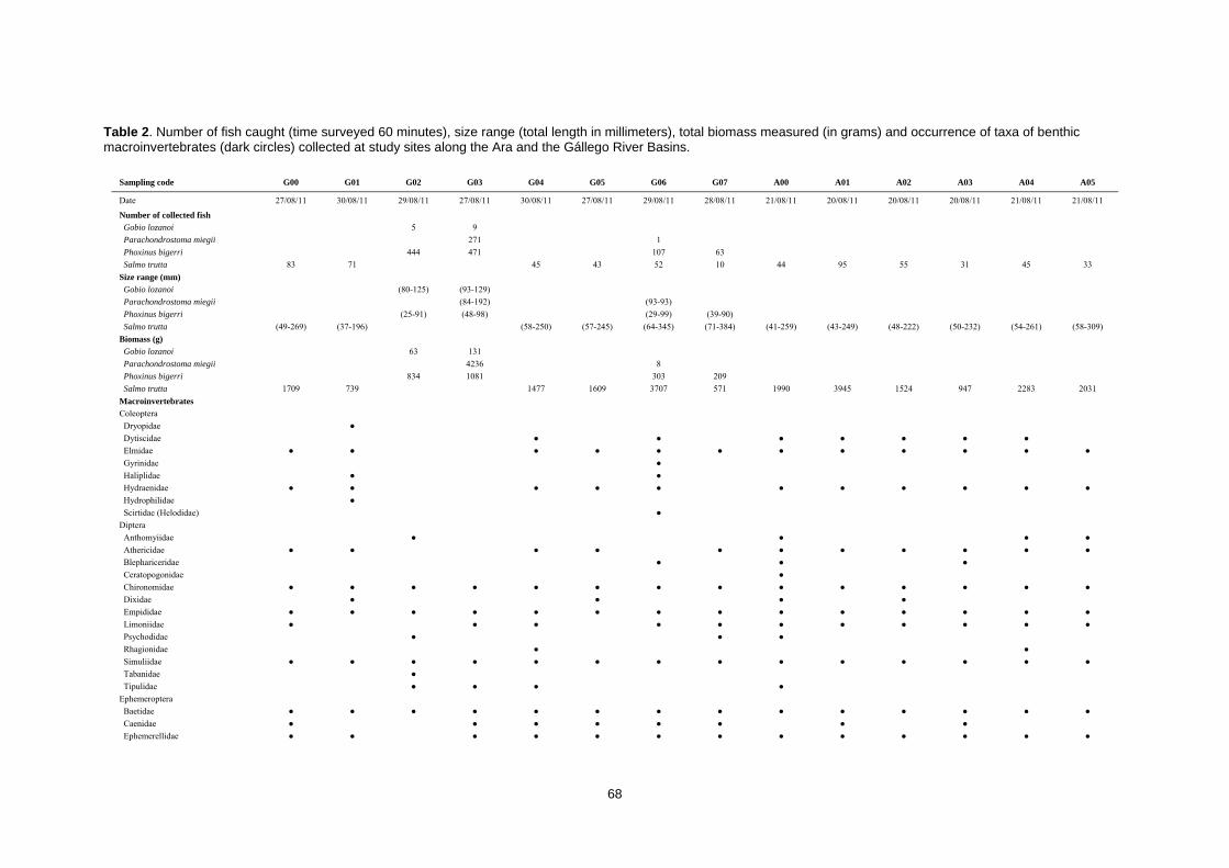
68
Table 2. Number of fish caught (time surveyed 60 minutes), size range (total length in millimeters), total biomass measured (in grams) and occurrence of taxa of benthic macroinvertebrates (dark circles) collected at study sites along the Ara and the Gállego River Basins.
Sampling code G00 G01 G02 G03 G04 G05 G06 G07 A00 A01 A02 A03 A04 A05
Date 27/08/11 30/08/11 29/08/11 27/08/11 30/08/11 27/08/11 29/08/11 28/08/11 21/08/11 20/08/11 20/08/11 20/08/11 21/08/11 21/08/11
Number of collected fish
Gobio lozanoi 5 9
Parachondrostoma miegii 271 1
Phoxinus bigerri 444 471 107 63
Salmo trutta 83 71 45 43 52 10 44 95 55 31 45 33
Size range (mm)
Gobio lozanoi (80-125) (93-129)
Parachondrostoma miegii (84-192) (93-93)
Phoxinus bigerri (25-91) (48-98) (29-99) (39-90)
Salmo trutta (49-269) (37-196) (58-250) (57-245) (64-345) (71-384) (41-259) (43-249) (48-222) (50-232) (54-261) (58-309)
Biomass (g)
Gobio lozanoi 63 131
Parachondrostoma miegii 4236 8
Phoxinus bigerri 834 1081 303 209
Salmo trutta 1709 739 1477 1609 3707 571 1990 3945 1524 947 2283 2031
Macroinvertebrates
Coleoptera
Dryopidae ●
Dytiscidae ● ● ● ● ● ● ●
Elmidae ● ● ● ● ● ● ● ● ● ● ● ●
Gyrinidae ●
Haliplidae ● ●
Hydraenidae ● ● ● ● ● ● ● ● ● ● ●
Hydrophilidae ●
Scirtidae (Helodidae) ●
Diptera
Anthomyiidae ● ● ● ●
Athericidae ● ● ● ● ● ● ● ● ● ● ●
Blephariceridae ● ● ●
Ceratopogonidae ●
Chironomidae ● ● ● ● ● ● ● ● ● ● ● ● ● ●
Dixidae ● ● ● ●
Empididae ● ● ● ● ● ● ● ● ● ● ● ● ● ●
Limoniidae ● ● ● ● ● ● ● ● ● ● ●
Psychodidae ● ● ●
Rhagionidae ● ●
Simuliidae ● ● ● ● ● ● ● ● ● ● ● ● ● ●
Tabanidae ●
Tipulidae ● ● ● ●
Ephemeroptera
Baetidae ● ● ● ● ● ● ● ● ● ● ● ● ● ●
Caenidae ● ● ● ● ● ● ● ●
Ephemerellidae ● ● ● ● ● ● ● ● ● ● ● ● ●
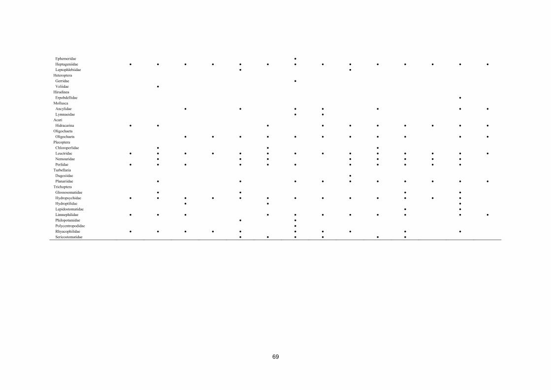
69
Ephemeridae ●
Heptageniidae ● ● ● ● ● ● ● ● ● ● ● ● ● ●
Leptophlebiidae ● ●
Heteroptera
Gerridae ●
Veliidae ●
Hirudinea
Erpobdellidae ●
Mollusca
Ancylidae ● ● ● ● ● ● ●
Lymnaeidae ● ●
Acari
Hidracarina ● ● ● ● ● ● ● ● ● ●
Oligochaeta
Oligochaeta ● ● ● ● ● ● ● ● ● ● ●
Plecoptera
Chloroperlidae ● ● ●
Leuctridae ● ● ● ● ● ● ● ● ● ● ● ● ● ●
Nemouridae ● ● ● ● ● ● ● ●
Perlidae ● ● ● ● ● ● ● ● ● ● ●
Turbellaria
Dugesiidae ●
Planariidae ● ● ● ● ● ● ● ● ● ●
Trichoptera
Glossosomatidae ● ● ● ●
Hydropsychidae ● ● ● ● ● ● ● ● ● ● ● ● ●
Hydroptilidae ● ● ●
Lepidostomatidae ● ●
Limnephilidae ● ● ● ● ● ● ● ● ● ● ●
Philopotamidae ● ●
Polycentropodidae ●
Rhyacophilidae ● ● ● ● ● ● ● ● ● ●
Sericostomatidae ● ● ● ● ● ●
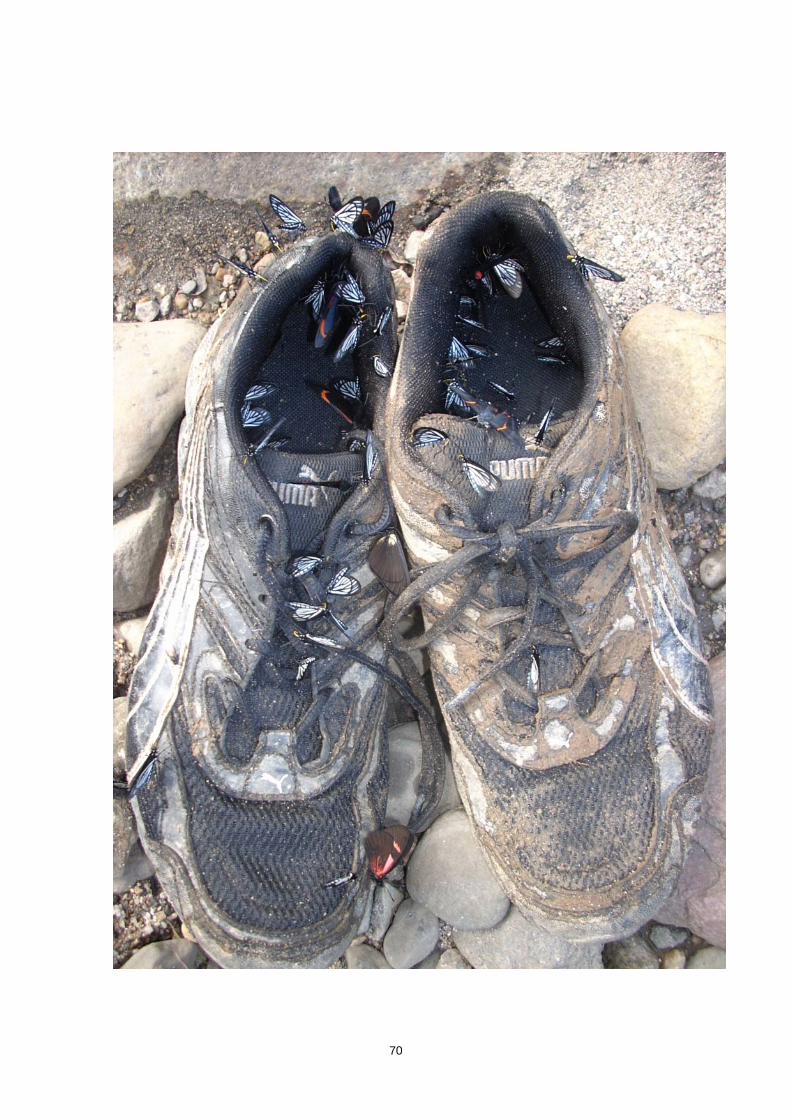
70
71
CAPÍTULO 2ND CHAPTER PATRONES DE DISTRIBUCIÓN ESPACIAL DE LAS COMUNIDADES DE PECES RELATIVOS A LOS MACROINVERTEBRADOS Y LAS CONDICIONES AMBIENTALES EN RÍOS DEL PIEDEMONTE DE LA AMAZONÍA COLOMBIANA Spatial distribution patterns of fish assemblages relative to macroinvertebrates and environmental conditions in Andean piedmont streams of the Colombian Amazon
Tobes I, Gaspar S, Peláez‐Rodríguez M, Miranda R
Inland Waters, 6: 89‐104 (2016)

72
73
Resumen
El presente trabajo ofrece una visión única de la biodiversidad y los procesos ecológicos de
unos ecosistemas neotropicales de agua dulce apenas estudiados. El río Hacha, situado al
suroeste de Colombia, en el piedemonte andino-amazónico, alberga una biodiversidad rica y
desconocida y está sufriendo la creciente influencia de los impactos humanos causados por la
ciudad de Florencia. Se analizaron los cambios en las características naturales del hábitat y la
calidad del medio ambiente y se relacionaron con la distribución de los peces y
macroinvertebrados. Se aplicaron cuatro índices de calidad ambiental y se midieron las
concentraciones de potenciales contaminantes del agua. Todos los índices de calidad ambiental
utilizados mostraron su fiabilidad, ya que evaluaron de forma conjunta y coherente la
integridad ecológica de los sitios de estudio y fueron inversamente proporcionales a las
posibles concentraciones de contaminantes del agua. Las comunidades de peces y de
macroinvertebrados cambiaron notablemente en respuesta a las diferencias en la calidad
ambiental, reforzando las evaluaciones de integridad ecológica. Sin embargo, los gradientes
naturales que influyen en las distribuciones de peces y macroinvertebrados mostraron una
superposición con los cambios en la calidad ambiental. Esta superposición enmascaró las
influencias de las alteraciones naturales confundiéndolas con las alteraciones provocadas por
el hombre, lo cuál limita nuestra capacidad de discernir entre ambas y atribuir a las
alteraciones de hábitat los notables cambios observados en los grupos de peces.
Palabras clave: ríos neotropicales, Colombia, contaminación del agua, evaluación del estado
ecológico, distribución piscícola, impacto humano, seguimiento biológico.
74
Abstract
The present work provides unique insight into an Andean-Amazonian river system by
conducting a comprehensive study of the biodiversity and ecological processes in a poorly
studied neotropical freshwater ecosystem. Hacha River, in western Colombia, harbours a rich
and unknown biodiversity and is experiencing an increase in human impacts from the city of
Florencia. Changes in natural habitat characteristics and environmental quality were analysed
and related to the distribution of fish and macroinvertebrates. Four environmental quality
indices were applied and concentrations of potential water pollutants were measured. All
environmental quality indices used were reliable, as they produced similar assessments of the
ecological integrity of the study sites and were inversely related to the potential water pollutant
concentrations. Fish and macroinvertebrate communities notably changed in response to
differences in environmental quality reinforcing the ecological integrity assessments.
Nevertheless, natural gradients that influence fish and macroinvertebrate distributions showed
an overlap with changes in environmental quality thereby confounding the ability to discern the
influence of natural and human-induced alterations and to confirm an initial shift in fish
assemblages due to anthropogenic impacts.
Key words: Neotropical stream, Colombia, water pollution, environmental quality indices, fish
assemblages, human impact, biomonitoring.
75
Introduction
Freshwater ecosystems are among the most threatened systems and are
especially vulnerable to degradation from anthropogenic activities (Vörösmarty et al.
2010). In this respect, knowledge of species distribution and diversity patterns are
crucial for developing conservation strategies, especially when focal species are
threatened or endangered. Unfortunately, knowledge on species diversity is still low in
some geographic areas. In particular, fish assemblage distribution in mountain streams
of the Andes are poorly understood, where only a few descriptive studies have been
conducted (e.g. Barthem et al. 2003, Maldonado-Ocampo et al. 2005).
Colombia harbours more than 10% of total global biodiversity; however, it
represents only 0.7% of the planetary surface (McNeely et al. 1990). This makes
Colombia among the top five countries in the world with respect to biodiversity.
Although detailed biological inventories for the entire Colombian territory are not yet
available, evidence suggests that the highest biodiversity occurs in the piedmonts of
mountain ranges (Romero et al. 2008). These territories belong to the tropical Andes
biodiversity hotspots for conservation priority due to the exceptional number of
endemic species experiencing habitat loss (Myers et al. 2000). Furthermore, expansive
areas of the tropical Andes still remain poorly studied, potentially concealing an
enormous and unknown biological richness (Romero et al. 2008).
There are 1435 described fish species inhabiting freshwater ecosystems in
Colombia, and 311 are endemic to the country. The Amazonian hydrographical system
is the main source of this biological richness (Maldonado-Ocampo et al. 2008).
Although the study of fishes in the Amazon Basin in Colombia has a long history
beginning at the end of the 19th century, most major water bodies still remain
unexplored, and consequently, species richness is most likely underestimated (Bogotá-
Gregory and Maldonado-Ocampo 2006).
One of the central tasks of freshwater research is to identify and explain how
environmental gradients configure the distribution and abundance of organisms along a
stream (Vannote et al. 1980, Schlosser 1991, Ward et al. 2002). Studies on stream
synecology have emphasised this relationship between species and their changing
environment as a prerequisite for species conservation and land management (Allan
76
2004). Organisms are influenced by numerous drivers operating at multiple spatial
scales (e.g. topography, geology) and landscape scale (e.g. climate). These drivers
determine factors at smaller scales, including type and availability of energy resources,
physical habitat or hydrochemical characteristics (Allan et al. 1997).
Biological communities are sensitive indicators of the relative health of aquatic
ecosystems and the surrounding catchment (Fausch et al. 2002, Allan 2004, Hering et
al. 2006). The use of macroinvertebrates is widely recognised as a biological monitoring
tool due to their sensitive response to changes in environmental conditions and the
biotic indices obtained from macroinvertebrates are accepted as reliable environmental
quality indicators (Bonada et al. 2006, Friberg et al. 2011). Similarly, fish also are
potentially effective indicators of aquatic ecosystem conditions because different
species exhibit diverse ecological, morphological, physiological and behavioural
adaptations to their natural habitat. Numerous studies have demonstrated the
bioindicator potential of fish communities (Karr 1981, Matthews and Hough 1992, Joy
and Death 2002, Hued and Bistoni 2005).
Human activities at the landscape scale have been increasingly recognised as a
major threat to the ecological integrity of river ecosystems, impacting habitat, water
quality, and biota via numerous and complex pathways (Allan et al. 1997, Bojsen and
Barriga 2002, Habit et al. 2006). Agriculture, cattle-raising and urbanisation represent
important sources of environmental impacts to riverine landscapes, as they are
responsible for major changes in the hydrochemical parameters of rivers. Organic
enrichment caused by these activities is a major threat (Hellawell 1986, Friberg et al.
2011). Some studies report changes in fish community composition and species
abundance below areas of concentrated anthropogenic impacts, proving their value as
human impact indicators (e.g., Lyons et al. 1995, Ortega et al. 2010b). Nevertheless, a
general response model does not exist (Paul and Meyer 2001), especially for the
neotropical region where relevant information is even more scarce (Alexandre et al.
2010).
The eastern Andean piedmont is a rapidly changing landscape where the recent
growth of human populations and the exploitation of natural resources have led to
extensive reductions in native vegetation and subsequent impacts on river habitats
(Brooks et al. 2002).
77
The main goal of this study is to achieve a better understanding of the local
ichthyofauna, examining how environmental variables and anthropogenic perturbations
affect and structure fish and macroinvertebrate assemblages, with the aim of identifying
patterns of association between fish assemblages and habitat variables, including human
activities. Several environmental quality indices were used to assess the presence and
intensity of human impacts. Although these indices are effective and widely used in
temperate regions, they are just starting to be applied in neotropical areas (Roldán,
2003; Acosta et al., 2009; Kutschker et al., 2009; Sirombra and Mesa, 2012), therefore
the reliability of the adapted versions of these indices was tested.
Materials and methods
Study area
This study was conducted along the Hacha River and its tributaries (Fig. 1). The
Hacha River Basin belongs to the Caquetá River Basin, the largest tributary of the
Amazon River in Colombia. The Hacha River Basin has a drainage area of 490 km2 and
the river flows 65 km south from its source at the peaks of the eastern Andes range
descending the piedmont to its confluence with the Orteguaza River in the Amazonian
plateau. Basin altitude ranges from 2575 m a.s.l. at the highest reach to 240 m a.s.l. at
the lowest point. The mean annual discharge is 35.7 m3 s-1, with a maximum value of
59.2 m3 s-1 in July and a minimum of 18.8 m3 s-1 in January (Rincón and Olarte, 2005).
The Hacha River runs through Florencia, the capital city of the Caquetá region,
and is the only substantial settlement in the basin with an estimated 167 000 inhabitants
and an annual population growth rate of 1.9% (Rincón and Olarte, 2005). The city,
founded in 1902, has experienced very rapid growth in an area that remained almost
pristine a century ago; therefore, its expansion represents a major impact to the area.
The city lacks a wastewater treatment plant, and consequently, all residential waters
flow directly into the river system without any prior treatment. The principal sewage
discharge is located upstream of the Q15 study site (Fig. 1) and represents a major
environmental impact. Other, smaller sewage outflows are located near study site Q16
and in the stretch of river between the H09 and H12 study sites.
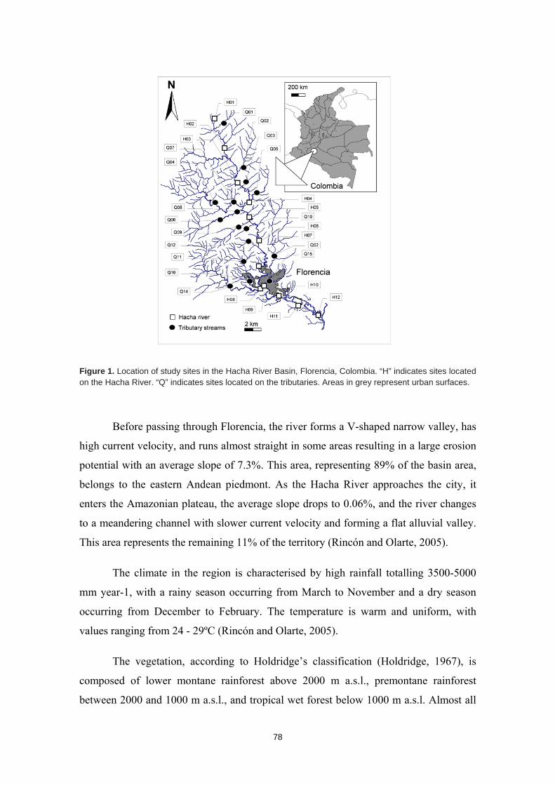
78
Figure 1. Location of study sites in the Hacha River Basin, Florencia, Colombia. “H” indicates sites located on the Hacha River. “Q” indicates sites located on the tributaries. Areas in grey represent urban surfaces.
Before passing through Florencia, the river forms a V-shaped narrow valley, has
high current velocity, and runs almost straight in some areas resulting in a large erosion
potential with an average slope of 7.3%. This area, representing 89% of the basin area,
belongs to the eastern Andean piedmont. As the Hacha River approaches the city, it
enters the Amazonian plateau, the average slope drops to 0.06%, and the river changes
to a meandering channel with slower current velocity and forming a flat alluvial valley.
This area represents the remaining 11% of the territory (Rincón and Olarte, 2005).
The climate in the region is characterised by high rainfall totalling 3500-5000
mm year-1, with a rainy season occurring from March to November and a dry season
occurring from December to February. The temperature is warm and uniform, with
values ranging from 24 - 29ºC (Rincón and Olarte, 2005).
The vegetation, according to Holdridge’s classification (Holdridge, 1967), is
composed of lower montane rainforest above 2000 m a.s.l., premontane rainforest
between 2000 and 1000 m a.s.l., and tropical wet forest below 1000 m a.s.l. Almost all
79
forests above 1000 m a.s.l. remain in good conservation status, as they are protected as
part of the “Amazonian Forest Reserve” representing 47.4% of the basin area. Areas
below the limits of the forest reserve have suffered massive deforestation and only
scattered forest stands remain. The slash-and-burn technique has been widely used
along the basin to convert land for agriculture. Those lands are mainly used for cattle-
raising, which represents the primary economic activity of the region occupying the
19.9% of the territory. Agriculture is a minor activity in the basin represented by some
subsistence farming lands occupying only the 1.8% of the territory (Rincón and Olarte
2005).
Data collection
A total of 28 sites were sampled once in the Hacha River (12 sites) and its
tributaries (16 sites) located between 2132 and 248 m a.s.l. (Fig. 1) from December
2008 to February 2009. The sampling period comprised the stable dry season in the
tropical rainforest climate. Study sites were distributed along the catchment area at
approximately five kilometre intervals to provide a comprehensive view of the basin
and to detect changes along the altitudinal gradient. Nevertheless, the selection of sites
was strongly limited by the poor accessibility. Stream reaches at each site were chosen
on the basis of ease of sampling and to avoid the deepest areas and very high current
velocities. Water temperature (°C), dissolved oxygen (mg l-1), pH, and specific
conductance (µS cm-1) were measured at each sampling site with a multi-parameter
water quality monitoring system (WTW Multi 340i). To assess water quality, samples
were collected and analysed for ammonium (N–NH+4) (mg l-1), orthophosphate (PO43-)
(mg l-1), nitrate (NO-2) (mg l-1) and nitrites (NO-3) (mg l-1) using standard methods
(Bartram 1996). These parameters were selected as possible indicators of water
pollution (Pesce and Wunderlin 2000). Habitat structure was characterised at three
locations along each of five to ten cross transects (depending on habitat heterogeneity)
distributed along the stream reach. Habitat parameters included depth (m), current
velocity (m s-1), % tree canopy shading, and dominant substrate categorised as fines (<2
mm), gravels (2-64 mm), cobbles (65-256 mm), boulders (>256 mm) and bedrock and
concrete (Armantrout 1998).
80
Three environmental quality habitat-based indices were applied: the Qualitative
Habitat Evaluation Index (QHEI), the Andean adapted versions of the Fluvial Habitat
Index (“Indice de Habitat Fluvial” or IHF) and the Riparian Forest Quality Index
(“Qualitat del Bosc de Ribera” or QBR). The QHEI index (Rankin 1989) focuses on
physical features that affect fish communities and other aquatic life. The IHF index
(Acosta et al., 2009; Pardo et al., 2004) characterises the physical habitat of streams and
rivers and evaluates the relationship between habitat heterogeneity and the physical
variables of the stream channel. The QBR index (Acosta et al. 2009; Munné et al. 2003)
is an easy-to-use field method for assessing the habitat quality of riparian forests.
Fish sampling was conducted using a backpack electrofishing unit (Hans Grassl
model IG200/2D, 300-600 V, 0.2-2 A). Semi-quantitative surveys with a constant unit
of effort (60 minutes per survey) were conducted (Meador et al., 2003), yielding fish
densities by catch per unit effort (CPUE, number of specimens collected per hour).
In the laboratory, fish were preserved in alcohol (75%) and identified to species,
when possible, or to higher taxonomic levels (i.e., genus or family) when taxonomic
information was insufficient for a reliable identification. Fish were identified using
taxonomic keys and other published literature (Mojica et al., 2005, Galvis et al., 2006,
Maldonado-Ocampo et al., 2008, Gaspar et al., 2012) as well as the collaborative efforts
of L. C. Chaves (Universidad de la Amazonia), J. I. Mojica and G. Galvis (Universidad
Nacional de Colombia). Fish fauna of this area are not well known. Most species have
complex taxonomic relationships that are unclear at present, and researchers are not in
full agreement on their taxonomic status. For this reason, the nomenclatural assignments
of Eschmeyer (2013) were used.
Macroinvertebrate sampling was conducted for evaluating water quality and
applying the BMWP procedure (Biological Monitoring Working Party) (Armitage et al.
1983). The BMWP is a procedure for measuring water quality using macroinvertebrates
as biological indicators. This method is based on the principle that aquatic invertebrate
taxa have different tolerances to pollutants, so the presence/absence of invertebrate
families can provide an assessment of water quality.
Qualitative macroinvertebrate samples were collected at each sampling site. A
representative stream reach was selected and a total of 20 kicks were taken
81
proportionally distributed in all microhabitats present at the site (Barbour et al. 1999). A
hand-net (25 cm x 25 cm aperture, 100-µm-mesh size) was used for the collection.
Kick-net contents were checked and deposited periodically in 2 litre plastic jars to avoid
losing organisms by overflow from the net. Samples were preserved in 5% buffered
formaldehyde for later identification in the laboratory. Specimens were identified to the
family level and the adapted BMWP index for Andean rivers developed to Colombia
(BMWP/Col) was applied (Roldán 2003), obtaining water quality values for all
sampling sites.
Data analysis
Differences in habitat variables and environmental quality among sample sites
were explored using two Principal Components Analyses (PCA), one assessing
variation of natural habitat characteristics across all sites, and one assessing
environmental quality across all sites. The first PCA for natural habitat characteristics
was applied using a combined matrix including hydrochemical parameters (temperature,
dissolved oxygen, pH, and conductivity) and habitat structure characteristics (mean
depth, water velocity, substrate type, and % canopy cover ) (Table 1). The second PCA
for environmental quality included concentrations of potential water pollution indicators
(nitrite, nitrate, ammonium and orthophosphates), hydrochemical parameters influenced
by anthropogenic alterations (temperature, conductivity, pH and dissolved oxygen)
(Pesce and Wunderlin, 2000) and scores from environmental and habitat quality indices
(IHF, QBR, QHEI, and BMWP/Col) (Table 1). Thus, two independent PCA analyses
were obtained to infer differences among sites for natural habitat characteristics and
environmental quality.
Shannon’s diversity (Shannon and Weaver, 1949) and Dominance indices
(Landau, 1951) for fish were estimated and the Bray-Curtis index of similarity was
used to compare fish and macroinvertebrate assemblages between study sites. A matrix
of abundances was used for studying fish community clustering using PAST statistical
software (Hammer et al., 2001) (Table 2). For macroinvertebrates, the matrix included
the presence/absence of families found at each site. This analysis provides a different
approach for studying the potential habitat distribution inferred from the similarity and
grouping of sites, and highlights different habitat ranges exclusively related to the
faunistic assemblages.
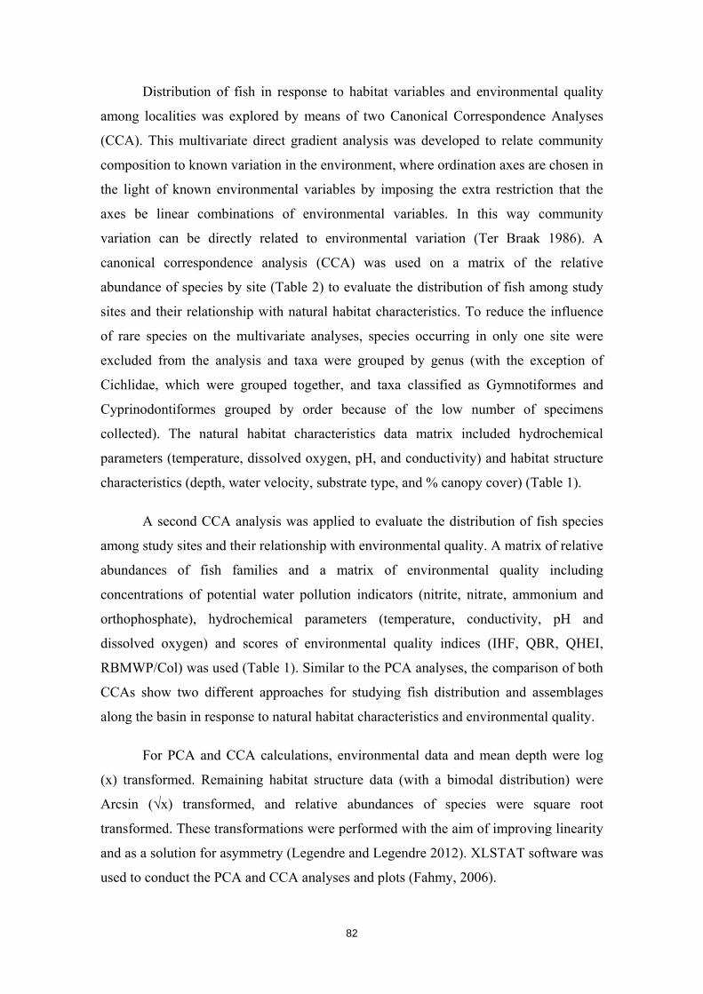
82
Distribution of fish in response to habitat variables and environmental quality
among localities was explored by means of two Canonical Correspondence Analyses
(CCA). This multivariate direct gradient analysis was developed to relate community
composition to known variation in the environment, where ordination axes are chosen in
the light of known environmental variables by imposing the extra restriction that the
axes be linear combinations of environmental variables. In this way community
variation can be directly related to environmental variation (Ter Braak 1986). A
canonical correspondence analysis (CCA) was used on a matrix of the relative
abundance of species by site (Table 2) to evaluate the distribution of fish among study
sites and their relationship with natural habitat characteristics. To reduce the influence
of rare species on the multivariate analyses, species occurring in only one site were
excluded from the analysis and taxa were grouped by genus (with the exception of
Cichlidae, which were grouped together, and taxa classified as Gymnotiformes and
Cyprinodontiformes grouped by order because of the low number of specimens
collected). The natural habitat characteristics data matrix included hydrochemical
parameters (temperature, dissolved oxygen, pH, and conductivity) and habitat structure
characteristics (depth, water velocity, substrate type, and % canopy cover) (Table 1).
A second CCA analysis was applied to evaluate the distribution of fish species
among study sites and their relationship with environmental quality. A matrix of relative
abundances of fish families and a matrix of environmental quality including
concentrations of potential water pollution indicators (nitrite, nitrate, ammonium and
orthophosphate), hydrochemical parameters (temperature, conductivity, pH and
dissolved oxygen) and scores of environmental quality indices (IHF, QBR, QHEI,
RBMWP/Col) was used (Table 1). Similar to the PCA analyses, the comparison of both
CCAs show two different approaches for studying fish distribution and assemblages
along the basin in response to natural habitat characteristics and environmental quality.
For PCA and CCA calculations, environmental data and mean depth were log
(x) transformed. Remaining habitat structure data (with a bimodal distribution) were
Arcsin (√x) transformed, and relative abundances of species were square root
transformed. These transformations were performed with the aim of improving linearity
and as a solution for asymmetry (Legendre and Legendre 2012). XLSTAT software was
used to conduct the PCA and CCA analyses and plots (Fahmy, 2006).
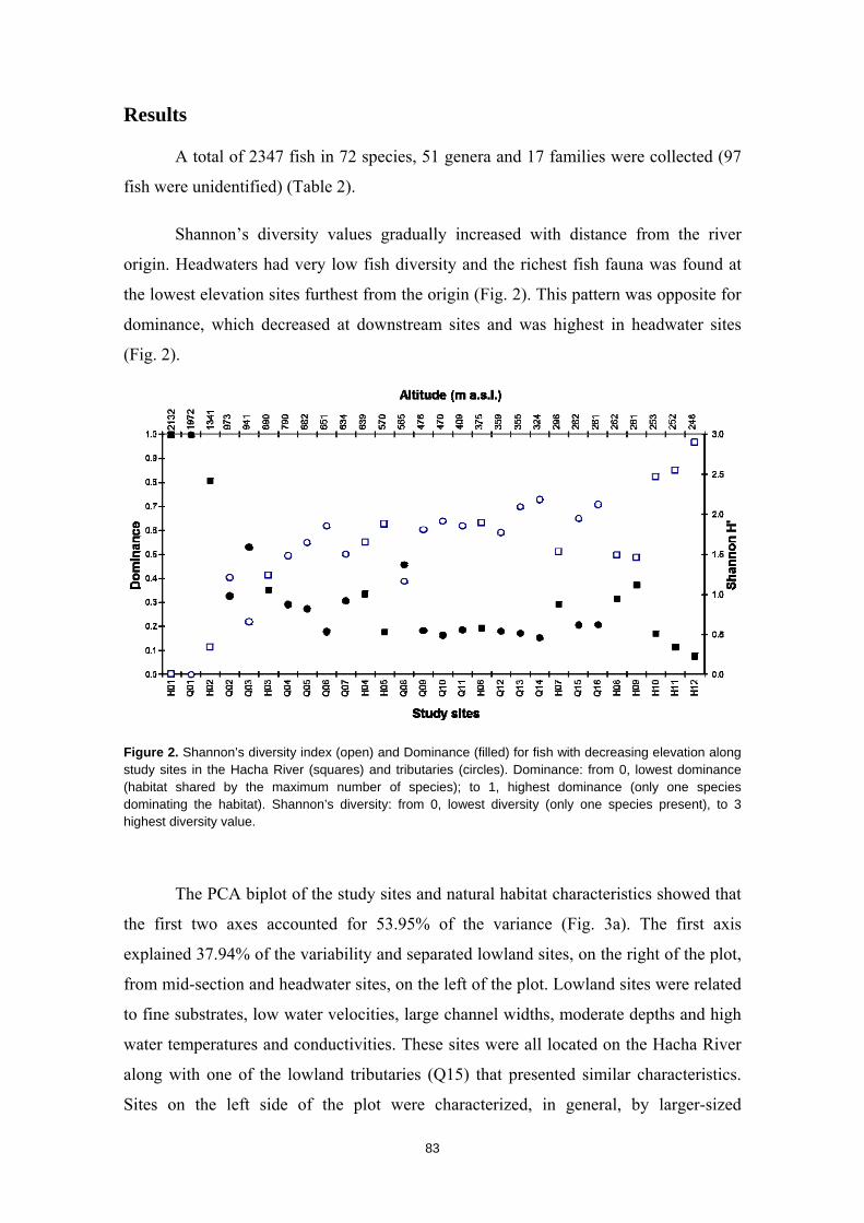
83
Results
A total of 2347 fish in 72 species, 51 genera and 17 families were collected (97
fish were unidentified) (Table 2).
Shannon’s diversity values gradually increased with distance from the river
origin. Headwaters had very low fish diversity and the richest fish fauna was found at
the lowest elevation sites furthest from the origin (Fig. 2). This pattern was opposite for
dominance, which decreased at downstream sites and was highest in headwater sites
(Fig. 2).
Figure 2. Shannon’s diversity index (open) and Dominance (filled) for fish with decreasing elevation along study sites in the Hacha River (squares) and tributaries (circles). Dominance: from 0, lowest dominance (habitat shared by the maximum number of species); to 1, highest dominance (only one species dominating the habitat). Shannon’s diversity: from 0, lowest diversity (only one species present), to 3 highest diversity value.
The PCA biplot of the study sites and natural habitat characteristics showed that
the first two axes accounted for 53.95% of the variance (Fig. 3a). The first axis
explained 37.94% of the variability and separated lowland sites, on the right of the plot,
from mid-section and headwater sites, on the left of the plot. Lowland sites were related
to fine substrates, low water velocities, large channel widths, moderate depths and high
water temperatures and conductivities. These sites were all located on the Hacha River
along with one of the lowland tributaries (Q15) that presented similar characteristics.
Sites on the left side of the plot were characterized, in general, by larger-sized
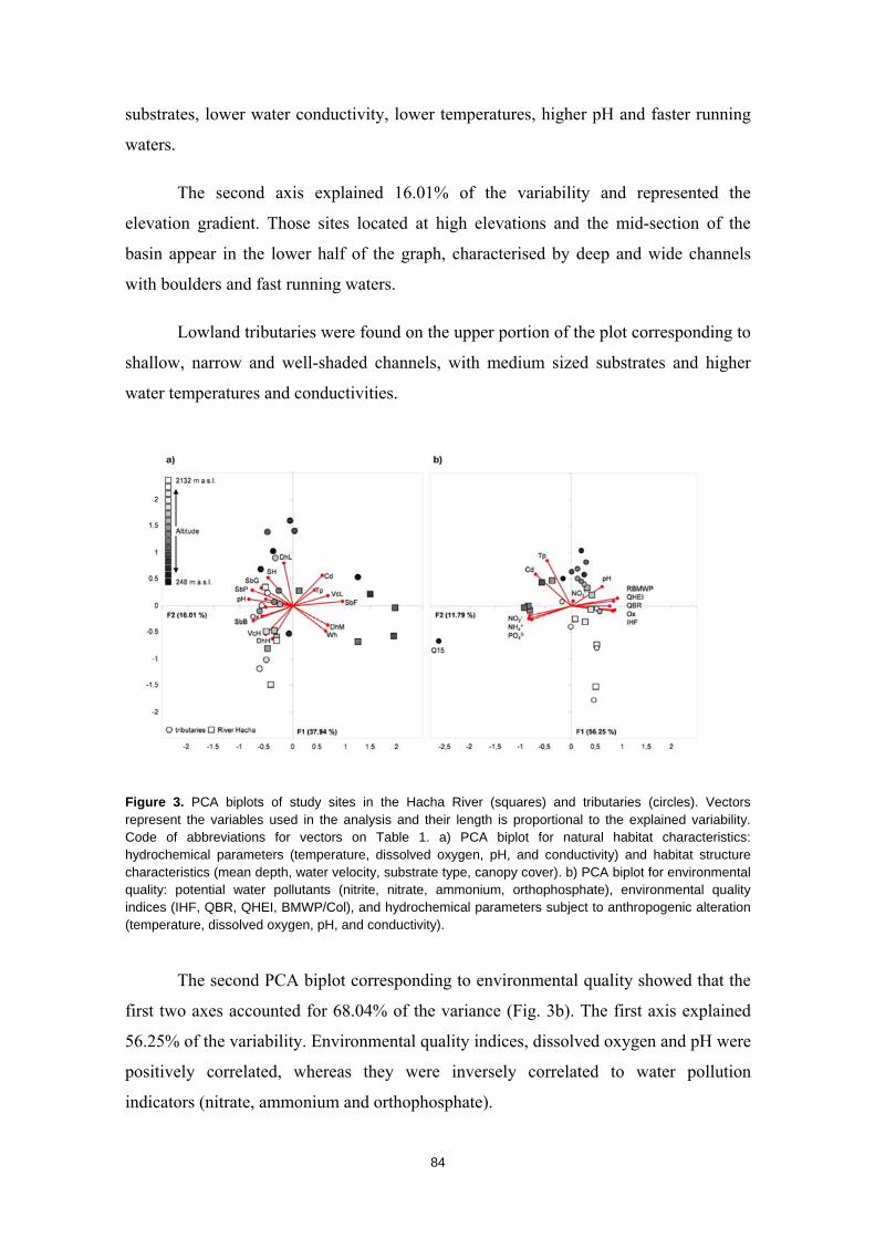
84
substrates, lower water conductivity, lower temperatures, higher pH and faster running
waters.
The second axis explained 16.01% of the variability and represented the
elevation gradient. Those sites located at high elevations and the mid-section of the
basin appear in the lower half of the graph, characterised by deep and wide channels
with boulders and fast running waters.
Lowland tributaries were found on the upper portion of the plot corresponding to
shallow, narrow and well-shaded channels, with medium sized substrates and higher
water temperatures and conductivities.
Figure 3. PCA biplots of study sites in the Hacha River (squares) and tributaries (circles). Vectors represent the variables used in the analysis and their length is proportional to the explained variability. Code of abbreviations for vectors on Table 1. a) PCA biplot for natural habitat characteristics: hydrochemical parameters (temperature, dissolved oxygen, pH, and conductivity) and habitat structure characteristics (mean depth, water velocity, substrate type, canopy cover). b) PCA biplot for environmental quality: potential water pollutants (nitrite, nitrate, ammonium, orthophosphate), environmental quality indices (IHF, QBR, QHEI, BMWP/Col), and hydrochemical parameters subject to anthropogenic alteration (temperature, dissolved oxygen, pH, and conductivity).
The second PCA biplot corresponding to environmental quality showed that the
first two axes accounted for 68.04% of the variance (Fig. 3b). The first axis explained
56.25% of the variability. Environmental quality indices, dissolved oxygen and pH were
positively correlated, whereas they were inversely correlated to water pollution
indicators (nitrate, ammonium and orthophosphate).
85
Study sites in the lower portion of the river were associated with low habitat
quality values (Fig. 3b). Among these sites, Q15 showed the most evident degradation.
In contrast, sites located on the right portion of the plot were characterised by high
habitat and water quality. The distribution along the second axis, explaining 11.79% of
the variability, was principally correlated with changes in water temperature,
conductivity and pH. Headwater sites were grouped on the bottom of the plot, mid-
section sites were distributed on the middle and lowland tributaries appeared on the top
of the plot.
Macroinvertebrate families along the study sites were separated into three main
groups by the Bray-Curtis similarity index (Fig. 4a). Sites corresponding to the upper
and middle locations on the basin appeared as a large unique group. Smaller clusters
were found within the larger cluster in response to the longitudinal location of sites
along the basin and corresponding to altitudinal ranges. Sites on the lowest areas of the
Hacha River formed a second group and were the same sites identified on the PCAs for
the lowest areas of the basin and the most impacted sites. Site Q15, grouped by the
PCAs with the sites on the lowest areas and showing the highest anthropogenic impact,
remained separated and alone in the cluster analysis, showing high dissimilarity to other
sites.
Cluster analysis of fish species using the Bray-Curtis similarity index (Fig. 4b)
matched the analysis of macroinvertebrates. Sites at the lowest areas were clustered
together as seen for macroinvertebrates and on the PCA analyses, and again, Q15
appeared different. The highest elevation headwater streams H01 and Q01 were similar
to each other but were different from the rest of sites.
Although Q15 was dissimilar from the rest of the sites in the cluster analyses of
macroinvertebrate and fish communities, this site was grouped with the lowland sites
with respect to fish, and showed no similarity with the rest of the sites and appeared
distinct with respect to macroinvertebrates (Fig. 4).
CCA plots (Fig. 5) exhibited a notable horseshoe deformation due to the high
number of fish groups included in the analysis; nevertheless, some distribution patterns
are evident. Permutation tests (1000 replicates) support the significance of the results (p
< 0.001). The first CCA (Fig. 5a), which related natural habitat characteristics and
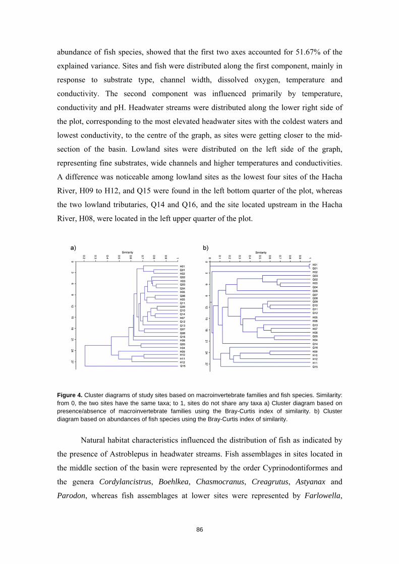
86
abundance of fish species, showed that the first two axes accounted for 51.67% of the
explained variance. Sites and fish were distributed along the first component, mainly in
response to substrate type, channel width, dissolved oxygen, temperature and
conductivity. The second component was influenced primarily by temperature,
conductivity and pH. Headwater streams were distributed along the lower right side of
the plot, corresponding to the most elevated headwater sites with the coldest waters and
lowest conductivity, to the centre of the graph, as sites were getting closer to the mid-
section of the basin. Lowland sites were distributed on the left side of the graph,
representing fine substrates, wide channels and higher temperatures and conductivities.
A difference was noticeable among lowland sites as the lowest four sites of the Hacha
River, H09 to H12, and Q15 were found in the left bottom quarter of the plot, whereas
the two lowland tributaries, Q14 and Q16, and the site located upstream in the Hacha
River, H08, were located in the left upper quarter of the plot.
Figure 4. Cluster diagrams of study sites based on macroinvertebrate families and fish species. Similarity: from 0, the two sites have the same taxa; to 1, sites do not share any taxa a) Cluster diagram based on presence/absence of macroinvertebrate families using the Bray-Curtis index of similarity. b) Cluster diagram based on abundances of fish species using the Bray-Curtis index of similarity.
Natural habitat characteristics influenced the distribution of fish as indicated by
the presence of Astroblepus in headwater streams. Fish assemblages in sites located in
the middle section of the basin were represented by the order Cyprinodontiformes and
the genera Cordylancistrus, Boehlkea, Chasmocranus, Creagrutus, Astyanax and
Parodon, whereas fish assemblages at lower sites were represented by Farlowella,
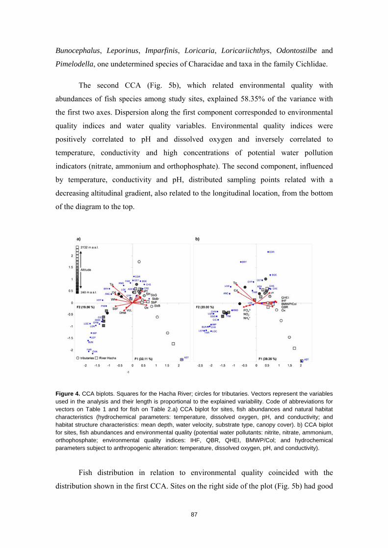
87
Bunocephalus, Leporinus, Imparfinis, Loricaria, Loricariichthys, Odontostilbe and
Pimelodella, one undetermined species of Characidae and taxa in the family Cichlidae.
The second CCA (Fig. 5b), which related environmental quality with
abundances of fish species among study sites, explained 58.35% of the variance with
the first two axes. Dispersion along the first component corresponded to environmental
quality indices and water quality variables. Environmental quality indices were
positively correlated to pH and dissolved oxygen and inversely correlated to
temperature, conductivity and high concentrations of potential water pollution
indicators (nitrate, ammonium and orthophosphate). The second component, influenced
by temperature, conductivity and pH, distributed sampling points related with a
decreasing altitudinal gradient, also related to the longitudinal location, from the bottom
of the diagram to the top.
Figure 4. CCA biplots. Squares for the Hacha River; circles for tributaries. Vectors represent the variables used in the analysis and their length is proportional to the explained variability. Code of abbreviations for vectors on Table 1 and for fish on Table 2.a) CCA biplot for sites, fish abundances and natural habitat characteristics (hydrochemical parameters: temperature, dissolved oxygen, pH, and conductivity; and habitat structure characteristics: mean depth, water velocity, substrate type, canopy cover). b) CCA biplot for sites, fish abundances and environmental quality (potential water pollutants: nitrite, nitrate, ammonium, orthophosphate; environmental quality indices: IHF, QBR, QHEI, BMWP/Col; and hydrochemical parameters subject to anthropogenic alteration: temperature, dissolved oxygen, pH, and conductivity).
Fish distribution in relation to environmental quality coincided with the
distribution shown in the first CCA. Sites on the right side of the plot (Fig. 5b) had good
88
environmental quality and were represented by Astroblepus, Creagrutus,
Chasmocranus, Boehlkea, Cordylancistrus and Astyanax, whereas sites on the left side
of the graph had habitat alteration and were represented by Farlowella, Bunocephalus,
Leporinus, Imparfinis, Loricaria, Loricariichthys, Odontostilbe and Pimelodella and
undetermined Characidae and Cichlidae.
Discussion
Two distinct regions were identified in the Hacha River Basin as a result of the
observed environmental gradients, the upper region, from the source at 2000 m a.s.l. to
approximately 300 m a.s.l., and the lower region, from approximately 300 m a.s.l. to its
confluence with the Orteguaza River. This zonation matches with the geomorphologic
changes occurring in the basin where the upper and middle sections are part of the
eastern Andean slopes, including sites from H01 to H07 in the Hacha River and
tributary streams from Q01 to Q14, and where the floodplain is on the Amazonian
plateau, represented by sites on the Hacha River between H08 and H12 and the Q15 and
Q16 tributary streams. The change in the geomorphology occurs abruptly near the city
of Florencia, changing from steep slopes to a flat plateau, and has a direct and major
influence on the hydromorphology of streams. The city of Florencia is located where
the transition occurs.
Changes in hydromorphology directly influence the biotic distribution and,
consequently, the structure and composition of fish assemblages in terms of
morphology and habitat use (Gorman and Karr, 1978; Matthews, 1998; Ward et al.,
2002; Jaramillo-Villa et al., 2010). Fish assemblages associated with river zonation are
evident, as the highest headwaters, lowland floodplains and the middle section sites
show corresponding fish groups, as indicated by CCA (Fig. 5) and Bray-Curtis
similarity analyses (Fig. 4).
The distributional range of freshwater fish species is related to a general increase
in the size and heterogeneity of habitats that provide more abundant and diverse food
resources and refuges (Matthews, 1998; Walters et al., 2003). This increase in habitat
diversity is directly related to changes in geomorphology, which can influence fish
community structure along altitudinal gradients (Robinson and Rand, 2005).
Environmental changes related to changes in geomorphology and the subsequent
response of the fish fauna was evident in the study area. Fish diversity along the Hacha
89
River Basin was highest in the lowest elevation sites corresponding to the floodplain
where the river becomes more suitable for a larger range of species and offers a wider
range of possible niches (e.g., Gorman and Karr, 1978).
Correspondingly, species richness decreased with increasing altitude and only a
few species increased in dominance. At the highest localities in the basin, Astroblepus
(climbing catfishes) were found to be strongly and exclusively related to the
headwaters, indicating turbulent, cold and highly oxygenated streams that still remain
almost pristine. This dominance of a few species at high altitudes seems to be a
compensating mechanism for adjusting populations to scarce available resources
(Matthews, 1998; Lomolino, 2001). Climbing catfishes occur in streams across a wide
range of elevations (100–4600 m) and ecosystems from Panama to Bolivia, with most
occurrences between 500 and 2000 m and associated principally with high elevation and
headwaters (Jaramillo-Villa et al., 2010; Schaefer and Arroyave, 2010; Anderson and
Maldonado-Ocampo, 2011).
Although limnological characteristics of rivers represent a major influence on
river ecosystems and subsequently on fish assemblages (Matthews and Hough, 1992)
due to increasing human uses of the land, anthropogenic influence is leading to a
notable alteration and degradation of riverine landscapes and is strongly affecting
natural distribution patterns (Booth and Jackson, 1997, Hering et al., 2006). Detecting
those impacts and their magnitude is crucial for guiding conservation efforts.
Environmental and water quality indices represent a valuable tool for identifying,
evaluating and locating human impacts and habitat degradation.
The values of the environmental quality indices QHEI, the Andean adaptations
of IHF and QBR and the adaptation of BMWP for Colombia agreed in their
environmental quality evaluation, identifying the same impacted sites. Although they
focus on different aspects of the river ecosystem, as one unique and complex
interrelated functional unit, the riverine landscape responds jointly to human influence,
so changes in one of the landscape components affects the others (Allan, 2004; Wiens,
2002). A deterioration in water quality was observed in the study sites affected by the
city of Florencia, where concentrations of potential anthropogenic water pollutants
(nitrate, nitrite, ammonium and orthophosphates) increased along with conductivity and
temperature, whereas dissolved oxygen concentration decreased, indicating a decline in
90
water quality due to sewage (Fig. 3b) (Pesce and Wunderlin, 2000). Therefore, the
inverse relationship between concentrations of potential water pollutants and scores for
environmental quality indices is consistent with the joint environmental quality
assessment. The concordance of selected water quality indicators and environmental
quality indices also supports the suitability of the selected parameters for detecting
water quality alterations.
Fish assemblages, as part of the riverine landscape, are intensely influenced by
human impacts and habitat degradation, so changes in fish assemblages are directly
related to the intensity and magnitude of these perturbations (Schlosser, 1991; Booth
and Jackson, 1997). This relationship is evident with the CCA analysis (Fig. 5b), where
various fish clusters were directly related to sites presenting different degrees of
anthropogenic influence, as Astroblepus appeared to be exclusively related to pristine
headwater sites, and cichlids, Bunocephalus, Imparfinis, Farlowella and Loricariichthys,
were found only in sites showing notable degradation. This group of fishes is associated
with areas of slow current velocity and low elevation extending into the Amazonian
plateau, and they are more tolerant of human impact than other Andean species (Reis et
al., 2003; Pouilly et al., 2006; Alexandre et al., 2010). Fish assemblages associate with
specific sites were also observed with the Bray-Curtis similarity analysis (Fig. 4b).
When compared to the macroinvertebrate similarity analysis (Fig. 4a), a noticeable
clustering was detected where the lowest areas of the basin were clustered together and
were dissimilar to the remaining sites.
In these same analyses, macroinvertebrate and fish communities corresponding
to the site experiencing the greatest and most direct anthropogenic effects, Q15, were
dissimilar from all other sites, although the difference was considerably greater for
macroinvertebrates (Fig. 4). Sites below H09, downstream of the confluence of the
Hacha River and the Q15 tributary, clustered together and were clearly separated from
the other sites. It is clear that the influence of polluted water entering the Hacha River
from Q15 affected both macroinvertebrate and fish populations (Coimbra et al., 1996;
Trujillo-Jiménez et al., 2010). Furthermore, due to the influence of this pollution source,
two sites occurring in close proximity appeared to be clearly distinct in both ordination
analyses. Site H09, located downstream of the confluence with Q15, receives polluted
water, and H08, located immediately upstream of the confluence, was not influenced by
91
the presence of sewage, and therefore presented healthier fish and macroinvertebrate
communities that was more similar to communities several kilometres upstream (at
H07) than to communities found a few meters downstream at H09 (Fig. 4).
The observed correlation between fish abundances and presence/absence,
macroinvertebrate distribution, and the BMWP/Col biotic index in response to
environmental quality indicates that fish have some predictive value as bioindicators
(Muotka et al., 1999; Carlisle et al., 2009). Nonetheless, although the fish and
macroinvertebrate cluster distributions and dissimilarity patterns were analogous, the
distinctiveness between sites and groups based on fish was less pronounced than for
macroinvertebrates. This suggests that macroinvertebrates may be more sensitive
indicators of water pollution than fish and, therefore, using macroinvertebrates as
bioindicators may be adequate for biomonitoring. Nevertheless, several studies have
found that macroinvertebrates are more sensitive to local habitat degradation than fish,
whereas fish are strongly correlated with land- use and catchment level variables,
emphasising the necessity of using both for conducting thorough environmental quality
assessments (Lammert and Allan, 1999; Freund and Petty, 2007).
Gradients of anthropogenic land-use are frequently superimposed on underlying
gradients of natural factors such as geology, soil type, topography, etc. (Allan, 2004).
This pattern was clearly observed along the Hacha River Basin. The part of the basin
located on the Andean slopes is characterised by narrow and V-shaped valleys with
steep slopes, which are less suitable for human land-use than floodplains with their flat
alluvial valleys. As a result, agriculture, cattle-raising and urbanisation occur in the
floodplain of the basin, concentrating the majority of human impacts below the H07
study site. The differences among Andean slopes and floodplain area not only affect
human settlement, it also noticeably influences streams and their environmental
characteristics, directly causing a significant change in fish diversity where the basin
becomes part of the Amazonian floodplains. Consequently, although fish community
changes related to anthropogenic impacts were observed (Alexandre et al., 2010), those
changes were also confounded by the distributional range of freshwater fish species
along the altitudinal gradients of the basin (Schlosser, 1991; Buisson et al., 2008). This
overlap of factors was apparent as the fish distributions shown by the CCA for natural
habitat characteristics (Fig. 5a) almost completely matched the CCA for environmental
92
quality indicators (Fig. 5b). Therefore, fish assemblages and distribution could not
solely be attributed to human impacts, as they overlapped with the natural change of
environmental variables. These results demonstrate the necessity of studying both
natural environmental conditions and those anthropogenically impacted to correctly
interpret information from faunal censuses. Ignoring important aspects such as habitat
or resource availability when using fish censuses for estimating environmental quality
or detecting the effects of anthropogenic disturbances can lead to misinterpretation of
the data, to the incorrect application of environmental quality indicators, and finally to
the implementation of inappropriate management decisions.
Although the application of environmental quality indices and the use of fish and
macroinvertebrates as bioindicators and as biomonitoring tools has been widely shown
to be useful for estimating ecological integrity in river ecosystems (Joy and Death,
2002; Leunda et al., 2009), the use of indices and fauna censuses must be combined
with a comprehensive knowledge of taxonomy, habitat requirements, and physiology of
the organisms being used as bioindicators. Furthermore, some studies show that changes
in fish assemblages do not occur immediately when human impacts begin but may take
many years of exposure, causing a gradual replacement of species (Fitzgerald et al.,
1998). This demonstrates the need for continued and prolonged monitoring, leading to
an accurate understanding and detection of changing fish assemblages (Appelberg et al.,
1995; Gutreuter et al., 1995).
Our results may show an initial shift of fish assemblages due to increasing
human impacts, but additional studies conducted in unimpacted rivers with similar
characteristics are necessary to verify if the observed patterns and fish assemblages
correspond to the presence of these impacts (Mercado-Silva et al., 2006; Carey and
Mather, 2008). Nevertheless, with further studies, fish assemblages might serve as an
important tool in the future to assess the condition of the environment or to diagnose the
causes of environmental changes.
Due to the paucity of information concerning neotropical fish biodiversity and
ecology and the few works studying the consequences of human impacts, it is difficult
to exclusively attribute observed changes in fish diversity to anthropogenic causes.
Consequently, if the goal is to develop adequate conservation policies and apply them
properly, there is a major need for additional research. A better understanding of the
93
wide range of processes occurring in riverine landscapes will allow us to quickly
identify potential threats and properly apply effective measures to control them.
Acknowledgments
This study was sponsored by the fellowship program III-B of the Ministry of
External Affairs of the Government of Spain (MAEC-AECID). The vice-rectory of
Research of the Universidad de la Amazonia provided logistic and economic resources
to complete this work. We are grateful to J. I. Mojica, G. Galvis (Universidad Nacional
de Colombia) and L. C. Chaves (Universidad de la Amazonia), who aided in the
identification of the fish; to D. Sierra, H. A. Peláez, Y. M. Salas, Y. A. Jara, D. Godoy,
C. A. Ospina and I. Sandoval, who assisted in fish collection and measurement; and to
A. F. Díaz, who helped with the SIG software and the cartography.
94
Table 1. Natural habitat characteristics and values for environmental quality estimation. “H” indicates sites on the Hacha River and “Q” indicates sites on the tributaries. Sampling points are ordered by altitude and distance from the origin. A column with the abbreviation codes for the variables is included.
Site Code H01 Q01 H02 Q02 Q03 H03 Q04 Q05 Q06 H04 Q07 H05 Q08 Q09
Coordinate (N) 1º52’40.7" 1º52’6.8" 1º50’2.6 1º47’41.4" 1º46’16.6" 1º46’28.8" 1º43’34.1" 1º44’55" 1º43’10" 1º44’38.0" 1º44’46" 1º43’33.7" 1º43’44.3" 1º42’42.2"
Coordinate (W) 75º40’44.1" 75º40’11.9" 75º40’4.7" 75º38’47.2" 75º38’21.3" 75º39’13.8" 75º40’3.6" 75º37’45" 75º39’54.3" 75º37’59.1" 75º78’34.5" 75º38’12.8" 75º7’49.5" 75º38’2.4"
Elevation (m) 2132 1972 1341 973 941 890 790 682 651 639 634 570 565 476
Water temperature (ºC) Tp 13.5 14.1 17.3 19.0 20.8 19.4 18.9 21.8 21.7 20.5 20.7 21.2 22.5 22.7
pH pH 7.1 7.1 7.3 7.3 7.3 7.7 7.1 7.4 7.4 7.4 7.3 7.3 7.4 7.5
Conductivity (μS cm-1) Cd 15.0 7.5 11.0 14.5 14.5 11.0 9.5 23.5 24.5 16.0 11.5 13.5 26.0 28.0
Dissolved Oxygen (mg l-1) Ox 10.60 8.12 8.10 8.27 8.27 8.34 8.40 7.93 8.00 8.39 8.27 8.39 7.92 8.24
Canopy cover (%) SH 83 33 33 10 44 0 40 21 24 27 80 8 67 33
Width mean (m) Wh 1.7 5 16 10 7 36 24 7 23 22 17 27 18 9
Depth
Low depth (%, <30 cm) DhL 42 62 33 19 57 13 20 63 43 33 40 42 21 33
Moderate depth (%, 30-60 cm) DhM 71 38 50 38 40 60 53 38 43 27 20 33 38 50
High depth (%, >60 cm) DhH 0 0 25 43 3 27 33 0 14 40 40 25 46 17
Water velocity
Low (%, <0.3 m s-1) VcL 25 38 42 14 30 20 27 33 43 27 33 17 33 28
Moderate (%, 0.3-0.75 m s-1) VcM 58 62 42 29 37 40 53 67 48 53 47 75 63 72
High (%, 0.75-1.2 m s-1) VcH 17 0 17 52 33 40 20 0 10 20 20 8 4 0
Substrate
Fines (%, <2 mm) SbF 0 13 14 3 1 11 6 8 9 9 8 18 15 13
Gravels (%, 2-64 mm) SbG 13 8 11 9 8 13 11 20 20 6 17 11 30 11
Pebbles (%, 64-256 mm) SbP 28 28 20 24 20 23 17 27 18 27 12 11 18 24
Boulders (%, >256 mm) SbB 22 25 35 47 35 47 35 20 30 14 5 18 13 23
Bedrock and concrete (%) SbBr 12 7 0 3 19 0 19 9 10 23 41 23 12 8
Chemical parameters
Nitrate (mg l-1) NO2- 0.531 0.366 0.493 0.736 0.531 0.689 0.336 0.303 1.687 0.372 1.961 1.459 1.459 0.107
Nitrites (mg l-1) NO3- 0.026 0.026 0.037 0.026 0.000 0.026 0.014 0.043 0.020 0.043 0.000 0.017 0.017 0.031
Ammonium (mg l-1) N-NH4+ 0.918 0.429 0.163 0.102 0.306 0.612 0.301 0.224 0.341 0.286 0.268 0.228 0.228 0.163
Orthophosphate (mg l-1) PO43- 0.013 0.083 0.017 0.022 0.002 0.017 0.008 0.057 0.007 0.025 0.005 0.018 0.018 0.053
Environmental indices
IHF IHF 66 73 71 62 70 63 81 57 71 66 79 68 66 64
QHEI QHEI 65 72 78 59 74 65 66 61 72 67 72 67 62 73
QBR QBR 100 90 100 30 100 65 100 70 80 65 90 95 80 95
RBMWP/Col RBMWP/Col 185 209 234 182 212 213 168 109 172 136 186 212 199 203
95
Site Code Q10 Q11 H06 Q12 Q13 Q14 H07 Q15 Q16 H08 H09 H10 H11 H12
Coordinate (N) 1º42’20.2" 1º38’58.7" 1º40’48.2" 1º40’48.4" 1º40’09.1" 1º36’22.6" 1º38’31.3" 1º36’34.2" 1º36’55.9" 1º36’21.9" 1º36’20" 1º35’39.1" 1º35’9.9" 1º33’19.2"
Coordinate (W) 75º37’39.6" 75º38’34.7" 75º37’18.9" 75º37’27.8" 75º35’47.3" 75º39’08.5" 75º37’3.6" 75º36’46.5" 75º37’40.8" 75º36’37" 75º36’32.4" 75º35’42.1" 75º33’19.6" 75º31’55"
Elevation (m) 470 409 375 359 355 324 296 282 281 262 261 253 252 248
Water temperature (ºC) Tp 23.6 24.1 22.1 24.0 24.4 25.3 22.4 25.4 24.9 25.1 24.0 23.6 23.9 24.5
pH pH 7.5 7.4 7.4 7.5 7.5 7.7 7.5 6.8 7.4 7.4 6.9 6.7 6.6 6.7
Conductivity (μS cm-1) Cd 36.0 30.5 16.5 33.0 22.0 27.0 15.5 55.5 27.5 26.5 32.0 29.0 29.0 34.0
Dissolved Oxygen (mg l-1) Ox 8.05 8.09 8.36 7.38 8.37 7.98 8.31 4.54 7.56 8.34 7.43 7.60 7.10 7.11
Canopy cover (%) SH 63 84 33 89 42 17 42 24 50 8 22 0 0 11
Width mean (m) Wh 4 9 30 6 17 27 68 21 12 69 70 120 90 100
Depth
Low depth (%, <30 cm) DhL 70 70 58 78 17 72 17 19 78 50 11 56 22 56
Moderate depth (%, 30-60 cm) DhM 23 30 8 22 58 28 42 67 28 50 78 56 89 56
High depth (%, >60 cm) DhH 7 4 33 0 25 0 42 14 0 0 11 0 0 0
Water velocity
Low (%, <0.3 m s-1) VcL 37 85 17 56 50 0 8 48 28 8 56 100 78 44
Moderate (%, 0.3-0.75 m s-1) VcM 63 15 33 44 33 78 83 52 50 67 44 0 22 56
High (%, 0.75-1.2 m s-1) VcH 0 0 50 0 17 22 8 0 22 25 0 0 0 0
Substrate
Fines (%, <2 mm) SbF 5 26 14 29 14 11 7 52 13 29 58 70 70 70
Gravels (%, 2-64 mm) SbG 21 21 0 2 3 19 6 15 17 25 0 0 0 0
Pebbles (%, 64-256 mm) SbP 31 23 0 20 25 38 27 10 36 35 0 0 0 0
Boulders (%, >256 mm) SbB 21 13 13 19 41 19 45 0 27 0 16 0 0 0
Bedrock and concrete (%) SbBr 0 5 49 8 0 4 0 0 4 0 0 0 0 0
Chemical parameters
Nitrate (mg l-1) NO2- 0.462 0.410 0.208 0.266 0.542 0.427 0.323 0.523 0.666 0.358 0.543 0.652 0.874 1.292
Nitrites (mg l-1) NO3- 0.046 0.006 0.000 0.034 0.011 0.011 0.000 0.100 0.026 0.057 0.057 0.040 0.049 0.023
Ammonium (mg l-1) N-NH4+ 0.163 0.082 0.041 0.224 0.612 0.000 0.061 3.673 1.551 0.673 2.082 1.020 0.980 0.367
Orthophosphate (mg l-1) PO43- 0.042 0.018 0.002 0.060 0.003 0.007 0.002 0.338 0.028 0.002 0.048 0.002 0.038 0.042
Environmental indices
IHF IHF 73 71 68 68 69 61 57 37 60 49 49 41 41 39
QHEI QHEI 79 73 70 69 66 66 70 36 67 54 54 40 40 50
QBR QBR 70 85 90 95 90 80 85 25 80 65 70 45 45 75
RBMWP/Col RBMWP/Col 187 212 149 162 183 197 159 9 168 107 72 61 111 120
96
Table 2. Relative abundances of fish species (catch per unit effort). “H” indicates sites located on the Hacha River and “Q” indicates sites located on the tributaries. Sampling points are ordered by altitude and distance from the origin. A column with abbreviation codes is included.
Code H01 Q01 H02 Q02 Q03 H03 Q04 Q05 Q06 Q07 H04 H05 Q08 Q09 Q10 Q11 H06 Q12 Q13 Q14 H07 Q15 Q16 H08 H9 H10 H11 H12 Total
Anostomidae Leporinus striatus Kner 1858 LEP 2 1 1 4
Characidae
Astyanax fasciatus Cuvier 1819 AST 4 7 11
Astyanax maximus Steindachner 1877 AST 1 1 7 12 2 1 24
Astyanax symmetricus Eigenmann 1908 AST 6 6
Astyanax sp1 Baird & Girard, 1854 AST 1 12 1 3 21 24 36 7 3 25 2 2 2 139
Astyanax sp2 Baird & Girard, 1854 AST 1 2 30 18 2 2 3 5 3 3 2 71
Astyanax sp3 Baird & Girard, 1854 AST 5 5
Boehlkea sp Géry 1966 BOE 2 7 1 6 1 30 44 42 10 28 11 4 1 187
Bryconamericus hypopterus Fowler 1943 BRY 16 1 2 19
Bryconamericus sp Eigenmann 1907 BRY 30 30
Ceratobranchia binghami Eigenmann 1927 CER 7 14 2 1 2 6 32
Creagrutus amoenus Fowler 1943 CRE 9 7 7 2 4 2 13 62 42 17 42 11 11 4 1 234
Creagrutus cochui Géry 1964 CRE 13 19 12 1 2 4 2 4 57
Creagrutus sp Günther 1864 CRE 3 10 13
Ctenobrycon hauxwellianus Cope 1870 CTE 2 12 14
Hemibrycon sp Günther 1864 HEB 24 24
Hemigrammus boesemani Géry 1959 HEG 2 2
Hyphessobrycon sp Durbin 1908 HYP 2 2
Knodus breviceps Eigenmann 1908 KNO 2 2
Knodus megalops Myers 1929 KNO 65 65
Moenkhausia robertsi Géry 1964 MOE 4 1 5
Odontostilbe fugitiva Cope 1870 ODO 4 4
Odontostilbe sp Cope 1870 ODO 2 11 4 10 1 28
Undetermined CHA 2 14 13 29
Crenuchidae
Characidium zebra Eigenmann 1909 CHM 1 6 3 1 1 9 21
Characidium sp1 Reinhardt 1867 CHM 5 2 2 8 14 2 3 3 4 4 2 49
Characidium sp2 Reinhardt 1868 CHM 11 11
Curimatidae
Steindachnerina bimaculata Steindachner 1876 STE 3 1 4
Erythrinidae
Hoplias malabaricus Bloch 1794 HOP 1 1 2
Parodontidae
Parodon pongoensis Allen 1942 PAR 3 1 4
97
Parodon sp Valenciennes 1850 PAR 1 1 1 1 3 1 8
Poeciliidae
Poecilia sp Bloch & Schneider 1801 CYP 1 5 2 1 9
Rivulidae
Rivulus sp Poey 1860 CYP 1 1 3 1 6
Apteronotidae
Apteronotus sp1 Lacepède 1800 GYM 3 2 5
Apteronotus sp2 Lacepède 1800 GYM 1 1 1 3
Platyurosternarchus macrostomus Günther 1870 GYM 2 2
Sternarchorhynchus sp Castelnau 1855 GYM 1 1
Rhamphichthyidae
Gymnorhamphichthys sp Ellis 1912 GYM 5 5
Sternopygidae
Eigenmannia virescens Valenciennes 1836 GYM 1 1 2
Sternopygus macrurus Bloch & Schneider 1801 GYM 1 2 1 2 6
Cichlidae
Aequidens sp Eigenmann & Bray 1894 CIC 1 11 4 2 4 7 1 30
Crenicichla sp Heckel 1840 CIC 2 2
Hypselecara temporalis Günther 1862 CIC 1 1
Aspredinidae
Bunocephalus spp Kner 1855 BUN 1 3 1 3 8
Astroblepidae
Astroblepus sp1 Humboldt 1805 AST 41 41
Astroblepus sp2 Humboldt 1805 AST 41 40 81
Astroblepus sp3 Humboldt 1805 AST 32 68 4 14 4 5 1 2 130
Heptapteridae
Cetopsorhamdia orinoco Schultz 1944 CET 1 5 25 14 33 10 14 22 124
Chasmocranus rosae Eigenmann 1922 CHS 3 1 3 3 1 15 22 1 14 63
Heptapterus sp Bleeker 1858 HEP 2 2
Imparfinis stictonotus Fowler 1940 IMP 6 5 7 18
Imparfinis sp Eigenmann & Norris 1900 IMP 1 3 1 2 7
Pimelodella conquetaensis Ahl 1925 PIM 3 7 18 1 49 37 1 6 122
Pimelodella spp Eigenmann & Eigenmann 1888 PIM 3 2 4 11 2 1 23
Rhamdia sp Bleeker 1858 RHA 1 1
Loricariidae
Ancistrus sp Kner 1854 ANC 4 9 5 18
Aposturisoma sp Isbrücker, Britski, Nijssen & Ortega 1983 APO 1 1
Chaetostoma alternifasciatum Fowler 1945 CHT 5 25 41 31 36 11 2 151
Chaetostoma sp Tschudi 1846 CHT 33 30 8 29 50 41 2 28 28 41 290
Cordylancistrus sp Isbrücker 1980 COR 1 19 20

98
Farlowella gracilis Regan 1904 FAR 1 12 22 8 43
Hypostomus plecostomus Linnaeus 1758 HYP 12 2 14
Hypostomus sp1 Lacepède 1803 HYP 2 1 3
Hypostomus sp2 Lacepède 1803 HYP 1 1
Lasiancistrus schomburgkii Günther 1864 LAS 3 3
Loricaria spp Linnaeus 1758 LOR 1 2 1 2 6
Loricariichthys sp Bleeker 1862 LOC 11 4 2 17
Otocinclus macrospilus Eigenmann & Allen 1942 OTO 1 1 2
Peckoltia vittata Steindachner 1881 PEC 2 2
Spatuloricaria sp Schultz 1944 SPA 2 2
Sturisoma sp Swainson 1838 STU 1 1
Sturisomatichthys sp Isbrücker & Nijssen 1979 STR 1 1 2
Synbranchidae 0
Synbranchus marmoratus Bloch 1795 SYN 1 1 2
99
CAPÍTULO 3RD CHAPTER RELACIONES LONGITUD‐PESO DE DIECISEIS PECES DE AGUA GULCE DEL RÍO HACHA Y SUS TRIBUTARIOS (CUENCA DEL AMAZONAS, CAQUETÁ, COLOMBIA) Length‐weight relationships of sixteen freshwater fishes from the Hacha River and its tributaries (Amazon Basin, Caquetá, Colombia)
Gaspar S, Tobes I, Miranda R, Leunda PM, Peláez M
Journal of Applied Ichthyology, 28: 667‐670 (2012)

100
101
Resumen
Se estimaron las relaciones del peso y la longitud corporal de dieciséis especies nativas de
peces (diez Characidae, tres Loricariidae, dos Heptapteridae y un Astroblepidae), todas ellas
especies de pequeño tamaño. Los muestreos se llevaron a cabo mediante pesca eléctrica en la
cuenca del río Hacha (Caquetá, Colombia), situada en el piedemonte andino-amazónico. Éstos
son los primeros parámetros longitud-peso y longitud-longitud registrados para estas especies,
principalmente endémicas de la cuenca amazónica. Además, en este estudio se registran las
máximas longitudes en ocho de las dieciséis especies. El conocimiento de estos datos
biométricos y sus relaciones pueden ser relevantes en la gestión y conservación de los recursos
pesqueros y la biodiversidad ictiológica local.
Palabras clave: peces endémicos, luz de malla, relaciones longitud-envergadura, gestión
pesquera local.
Abstract
Body lengths and weight relationships were estimated for sixteen native freshwater fish species,
(ten Characidae, three Loricariidae, two Heptapteridae and one Astroblepidae, mainly small-
sized fish) collected in the Andean piedmont Hacha River (Caquetá, Colombia) by
electrofishing. These are the first length-weight and length-length parameters reported for these
species, mostly endemic to the Amazonian basin. Besides, maximum lengths in eight of the
sixteen studied species are reported in this study. The knowledge of these biometric data and
relationships can be relevant in the management and conservation of local fish and fisheries.
Key words: endemic fishes, size mesh, girth-length relationships, local fisheries management.
102
Introduction
Inland freshwater fishery resources are exploited both commercially and for
subsistence in the Andean Amazon. Commercial fishing is carried out predominantly by
mobile and often urban-based professional fishermen, while subsistence fishing is
carried out locally by rural people resident in the riverside areas (Almeida and
Lorenzen, 2003).
The length-weight relationships (LWRs) of fishes are required in fishery
management and conservation because they are helpful to evaluate the production of
fish populations when only length measurements exists, enable the computation of
condition indexes and allow comparisons of species growth trajectories (between sexes,
seasons or regions) (Froese, 2006). In addition, relationships of total, standard and fork
lengths of fishes are also important in management for comparative growth studies
(Moutopoulos and Stergiou, 2002).
Besides, the morphological parameter of maximum girth is related to the
effectiveness of capture methods in fisheries (Jawad et al., 2009) because is the main
size factor determining the size of fish caught by different mesh sizes (Kurkilahti et al.,
2002). Good selection efficiency would lower the pressure on undersized fish, and
thereby increase the future size of exploitable stock (Grimaldo et al., 2008; Sistiaga et
al., 2009).
Few LWRs are known for freshwater fish species that are distributed in less-
studied areas (e.g., Hossain et al., 2009; Miranda et al., 2009). For example, according
to FishBase (Froese and Pauly, 2010) length-weight relationships have been determined
in this database for less than 8% of the native freshwater fish species registered in
Colombia. In fact, according to FishBase, none of the endemic freshwater fishes of
Colombia have published length-weight relationships.
Colombia is, after Brazil, the American country with the greatest freshwater fish
diversity, with more than 2,000 species, and the general knowledge on the biology of
these fishes is poor (Maldonado-Ocampo, 2006). Indeed, Colombia possesses the
highest diversity of mountain fishes within the Northern Andean region with 220
species, 37% of which are endemic (Jaramillo-Villa et al., 2010). In this area, fishes for
103
local consumption are caught with angling and traditional cast nets (atarraya in
Spanish).
In this paper we report the length-weight, length-length (total, standard and fork
length) and length-girth relationships of sixteen native freshwater fish species from the
Hacha River, in the (Caquetá, Colombia). Thirteen of them are endemic to the Amazon
basin and nine are endemic to the Upper Amazon (Colombia and Peru).
Materials and Methods
Sixteen freshwater fish species (ten Characidae, three Loricariidae, two
Heptapteridae and one Astroblepidae) were caught in the Hacha River and some little
tributaries (Amazon Basin, Colombia, 01º52’-01º33’ N and 75º31’-75º40’ W). Fish
specimens were obtained using a back-pack electrofishing unit (Hans-Grassl GmbH,
Model IG200-2C, voltage from 350 to 800 V and frequency from 35 to 100 pulses per
second) from November 2008 to March 2009. Twentyeight sites were sampled into the
Hacha River (12 sites) and their tributaries (16 sites). Altitude of sampling points varies
between 2132 m close to the source and 248 m near to its confluence with the River
Orteguaza (Amazon Basin).
Fish captured were anaesthetized with 2-phenoxyethanol, identified and
measured to the nearest 0.1 cm total length (TL), standard length (SL), fork length (FL),
height (HL) and width (WL). Subsequently, fish were weighted with a digital balance to
an accuracy of 0.05 g, before being returned to the river. In this study, both sexes have
been combined. Voucher specimens were euthanized by an overdose of anaesthesia and
transported to the laboratory for taxonomic verification.
In the laboratory, fishes were preserved in alcohol (75%) and identified using
taxonomic keys (Maldonado-Ocampo et al., 2005; Mojica et al., 2005; Galvis et al.,
2006) and the collaboration of L. C. Chaves (Universidad de la Amazonia), J. I. Mojica
and G. Galvis (Universidad Nacional de Colombia). Most of these species have
complex taxonomic relationships that presently are unclear, and researchers are not in
full agreement on their taxonomic status. For this reason, the nomenclatural assignments
of Eschmeyer (2010) were used. Once identified, specimens were deposited in the fish
collection of the Universidad de la Amazonia (Florencia, Colombia).
104
Length-weight relationships for all species were determined by the equation log
W = log a + b log TL, where W is the weight of the fish in grams, TL is the total length
in centimetres. Prior to regression analysis of log W on log TL, log–log plots of length
and weight values were performed for visual inspection of outliers. Only extreme
outliers attributed to data error were omitted from analyses (Froese, 2006). The length-
weight relationship calculated here is for adults and should not be used for juveniles
since it is likely that the relationship changes with maturity. Additionally, the b-value
for each species was tested by t-test to verify if it was significantly different from the
isometric growth (b = 3, Zar, 1999), where the body weight of fishes varies as the cube
of linear dimensions (Oscoz et al., 2005).
Maximum Girth (G) of fishes were obtained from the maximum height and
width, using the approximate formula proposed by Ramanujan in 1914 (Arfken and
Weber, 2000). Perimeter of ellipse (where minor and mayor radii are the maximum
height and width) is more accurate than maximum circumference to estimate the real
perimeter of body fish. The length-girth relationships (LGRs) between fish TL and
maximum girth were estimated by linear regression analysis: G = a + bTL.
Length-length relationships (LLRs) were also estimated by linear regression
analysis: TL = a + bFL and TL = a + bSL, where FL is the fork length and SL is the
standard length. Total and fork lengths relationship was not estimated for Chaetostoma
alternifasciatum, since caudal fin is truncated (Maldonado-Ocampo et al., 2005). In all
the regressions estimated, parameter a is the intercept and b the slope of the regression
line. The 95% confidence limits (CL) of b were calculated to estimate differences
between species (Zar, 1999).
Results
The size-class and the estimated parameters of the LWRs of the sixteen species
are given in Table 1. All LWRs were significant (p<0.01) with r2 values greater than
0.9, except for Boehlkea fredcochui (0.88). Farlowella gracilis, Pimelodella
conquetaensis, Boehlkea fredcochui, Chaetostoma alternifasciatum and Creagrutus
amoenus, showed significant positive-allometric growth (b > 3) and the remaining
species showed isometric growth (b = 3). The estimated parameters of the LGRs and
LLRs of the same species are presented in Table 2.
105
Discussion
The parameters of the calculated length-length, length-weight and length-girth
relationships can vary significantly according to sex and season (e.g., Kawamura, 1972;
Hossain et al., 2006), or due to other factors such as growth phase, stomach contents,
gonad development, habitat and health (e.g., Bagenal and Tesch, 1978; Leunda et al.,
2006). Since the individuals were collected over an extended period of time, these data
are not representative of a particular season or time of the year and for comparative
purposes should be considered only as mean annual values. Besides, positive allometric
growth has been widely reported in fishes, indicating an increase in relative body
fatness during the growth (Froese, 2006).
Gill and trammel nets selectivity are determined by girth and body length, along
with other biological and technical aspects as, for example, the existence of body
protuberances and spines, the fish behaviour, the mesh size or the hanging ratio (Santos
et al., 2006). Such is the case of the family Loricaridae (e.g. Chaetostoma
alternifasciatum or Cordylancistrus platyrhynchus) that presents pectoral and dorsal fin
spines that increase the gillnet capturability. Except for this family, girth is expected to
be more closely related to mesh size than length, because girth at the point of capture
has to be equal or slightly higher than the mesh perimeter for a fish to be retained.
Therefore, the information reported herein is particularly important for the management
of multispecies fisheries, which exploit a highly diversified fish fauna. This is the case
of the local Amazon fisheries, were practically all captured fish species by gill nets are
locally consumed.
To the authors’ best knowledge, this is the first published study in the consulted
literature that relates girths with other somatic measures in low commercial interest
freshwater fishes (Froese and Pauly, 2010). In spite of this, the knowledge of these
relationships has a relevant importance for management of local fisheries. These
relationships can avoid exploiting juveniles or immature specimens, using the correct
mesh size, providing the maintenance and the conservation of local fish populations.
However, the information presented in this study is preliminary and more detailed
studies are needed to answer several questions related to gillnet selectivity in inland
fisheries.
106
Acknowledgments
This study was sponsored by the fellowship program III-B of the Ministerio de
Asuntos Exteriores of the Government of Spain (MAEC-AECID). Vice-rectory of
Research of the Universidad de la Amazonia provided logistic and economics resources
for the achievement of this work. We are grateful to J. I. Mojica, G. Galvis (Universidad
Nacional de Colombia) and L. C. Chaves (Universidad de la Amazonia) who
collaborated in the fish’s identification; and to D. Sierra, H. A. Peláez, Y. M. Salas, Y.
A. Jara, D. Godoy, C. A. Ospina and I. Sandoval, who assisted in the collection and
measurement of the fish.
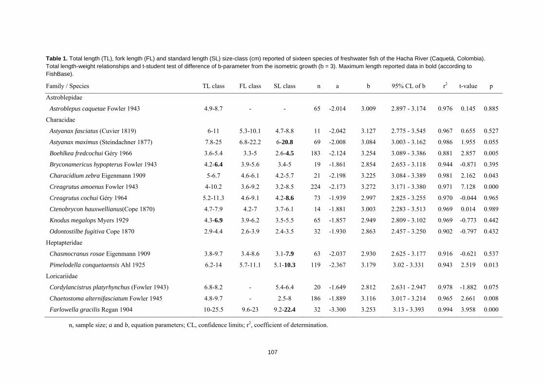
107
Table 1. Total length (TL), fork length (FL) and standard length (SL) size-class (cm) reported of sixteen species of freshwater fish of the Hacha River (Caquetá, Colombia). Total length-weight relationships and t-student test of difference of b-parameter from the isometric growth (b = 3). Maximum length reported data in bold (according to FishBase).
Family / Species TL class FL class SL class n a b 95% CL of b r2 t-value p
Astroblepidae
Astroblepus caquetae Fowler 1943 4.9-8.7 - - 65 -2.014 3.009 2.897 - 3.174 0.976 0.145 0.885
Characidae
Astyanax fasciatus (Cuvier 1819) 6-11 5.3-10.1 4.7-8.8 11 -2.042 3.127 2.775 - 3.545 0.967 0.655 0.527
Astyanax maximus (Steindachner 1877) 7.8-25 6.8-22.2 6-20.8 69 -2.008 3.084 3.003 - 3.162 0.986 1.955 0.055
Boehlkea fredcochui Géry 1966 3.6-5.4 3.3-5 2.6-4.5 183 -2.124 3.254 3.089 - 3.386 0.881 2.857 0.005
Bryconamericus hypopterus Fowler 1943 4.2-6.4 3.9-5.6 3.4-5 19 -1.861 2.854 2.653 - 3.118 0.944 -0.871 0.395
Characidium zebra Eigenmann 1909 5-6.7 4.6-6.1 4.2-5.7 21 -2.198 3.225 3.084 - 3.389 0.981 2.162 0.043
Creagrutus amoenus Fowler 1943 4-10.2 3.6-9.2 3.2-8.5 224 -2.173 3.272 3.171 - 3.380 0.971 7.128 0.000
Creagrutus cochui Géry 1964 5.2-11.3 4.6-9.1 4.2-8.6 73 -1.939 2.997 2.825 - 3.255 0.970 -0.044 0.965
Ctenobrycon hauxwellianus(Cope 1870) 4.7-7.9 4.2-7 3.7-6.1 14 -1.881 3.003 2.283 - 3.513 0.969 0.014 0.989
Knodus megalops Myers 1929 4.3-6.9 3.9-6.2 3.5-5.5 65 -1.857 2.949 2.809 - 3.102 0.969 -0.773 0.442
Odontostilbe fugitiva Cope 1870 2.9-4.4 2.6-3.9 2.4-3.5 32 -1.930 2.863 2.457 - 3.250 0.902 -0.797 0.432
Heptapteridae
Chasmocranus rosae Eigenmann 1909 3.8-9.7 3.4-8.6 3.1-7.9 63 -2.037 2.930 2.625 - 3.177 0.916 -0.621 0.537
Pimelodella conquetaensis Ahl 1925 6.2-14 5.7-11.1 5.1-10.3 119 -2.367 3.179 3.02 - 3.331 0.943 2.519 0.013
Loricariidae
Cordylancistrus platyrhynchus (Fowler 1943) 6.8-8.2 - 5.4-6.4 20 -1.649 2.812 2.631 - 2.947 0.978 -1.882 0.075
Chaetostoma alternifasciatum Fowler 1945 4.8-9.7 - 2.5-8 186 -1.889 3.116 3.017 - 3.214 0.965 2.661 0.008
Farlowella gracilis Regan 1904 10-25.5 9.6-23 9.2-22.4 32 -3.300 3.253 3.13 - 3.393 0.994 3.958 0.000
n, sample size; a and b, equation parameters; CL, confidence limits; r2, coefficient of determination.
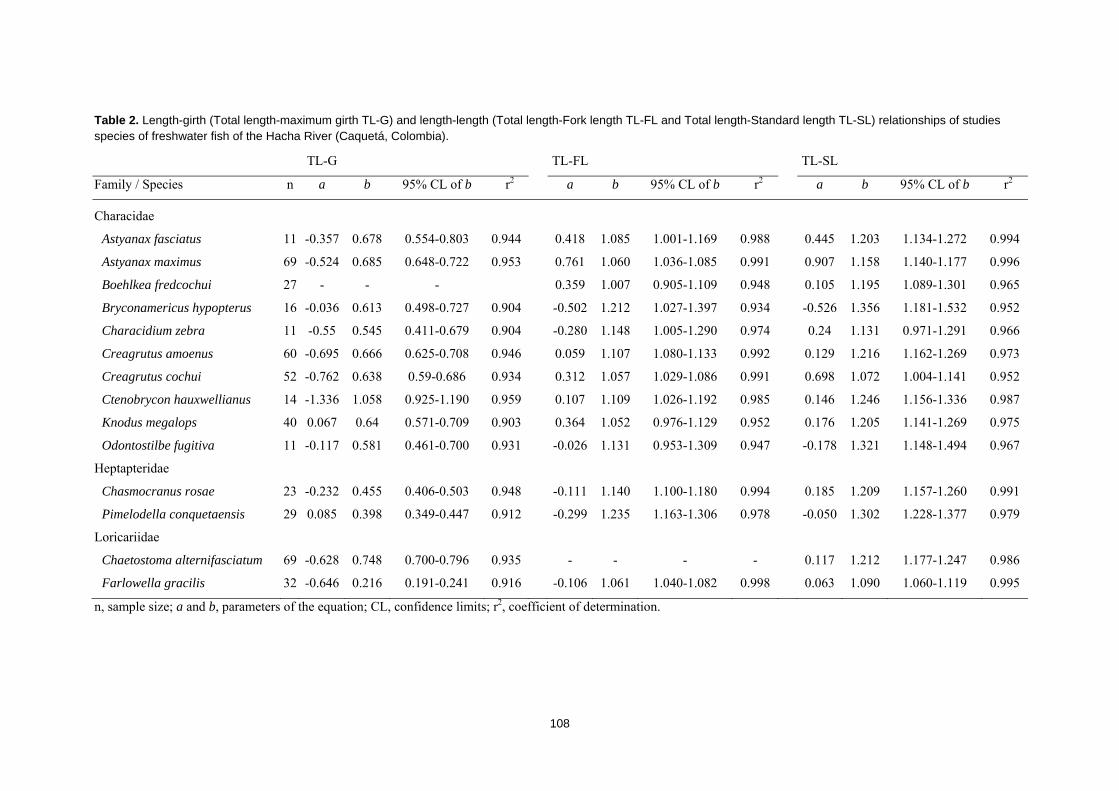
108
Table 2. Length-girth (Total length-maximum girth TL-G) and length-length (Total length-Fork length TL-FL and Total length-Standard length TL-SL) relationships of studies species of freshwater fish of the Hacha River (Caquetá, Colombia).
TL-G TL-FL TL-SL
Family / Species n a b 95% CL of b r2 a b 95% CL of b r2 a b 95% CL of b r2
Characidae
Astyanax fasciatus 11 -0.357 0.678 0.554-0.803 0.944 0.418 1.085 1.001-1.169 0.988 0.445 1.203 1.134-1.272 0.994
Astyanax maximus 69 -0.524 0.685 0.648-0.722 0.953 0.761 1.060 1.036-1.085 0.991 0.907 1.158 1.140-1.177 0.996
Boehlkea fredcochui 27 - - - 0.359 1.007 0.905-1.109 0.948 0.105 1.195 1.089-1.301 0.965
Bryconamericus hypopterus 16 -0.036 0.613 0.498-0.727 0.904 -0.502 1.212 1.027-1.397 0.934 -0.526 1.356 1.181-1.532 0.952
Characidium zebra 11 -0.55 0.545 0.411-0.679 0.904 -0.280 1.148 1.005-1.290 0.974 0.24 1.131 0.971-1.291 0.966
Creagrutus amoenus 60 -0.695 0.666 0.625-0.708 0.946 0.059 1.107 1.080-1.133 0.992 0.129 1.216 1.162-1.269 0.973
Creagrutus cochui 52 -0.762 0.638 0.59-0.686 0.934 0.312 1.057 1.029-1.086 0.991 0.698 1.072 1.004-1.141 0.952
Ctenobrycon hauxwellianus 14 -1.336 1.058 0.925-1.190 0.959 0.107 1.109 1.026-1.192 0.985 0.146 1.246 1.156-1.336 0.987
Knodus megalops 40 0.067 0.64 0.571-0.709 0.903 0.364 1.052 0.976-1.129 0.952 0.176 1.205 1.141-1.269 0.975
Odontostilbe fugitiva 11 -0.117 0.581 0.461-0.700 0.931 -0.026 1.131 0.953-1.309 0.947 -0.178 1.321 1.148-1.494 0.967
Heptapteridae
Chasmocranus rosae 23 -0.232 0.455 0.406-0.503 0.948 -0.111 1.140 1.100-1.180 0.994 0.185 1.209 1.157-1.260 0.991
Pimelodella conquetaensis 29 0.085 0.398 0.349-0.447 0.912 -0.299 1.235 1.163-1.306 0.978 -0.050 1.302 1.228-1.377 0.979
Loricariidae
Chaetostoma alternifasciatum 69 -0.628 0.748 0.700-0.796 0.935 - - - - 0.117 1.212 1.177-1.247 0.986
Farlowella gracilis 32 -0.646 0.216 0.191-0.241 0.916 -0.106 1.061 1.040-1.082 0.998 0.063 1.090 1.060-1.119 0.995
n, sample size; a and b, parameters of the equation; CL, confidence limits; r2, coefficient of determination.

109
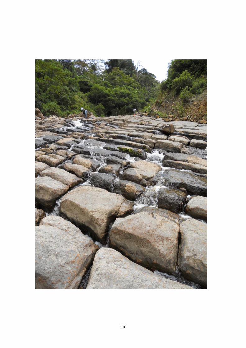
110
111
CAPÍTULO 4TH CHAPTER DISTRIBUCIÓN DE LAS COMUNIDADES DE PECES Y PATRONES AMBIENTALES A LO LARGO DE LA CUENCA DEL RÍO SUAZA (COLOMBIA): DESDE EL PARQUE NACIONAL NATURAL CUEVA DE LOS GUÁCHAROS HASTA LOS TERRITORIOS DE SU CUENCA BAJA Fish assemblage distribution and environmental patterns in the Suaza River Basin (Colombia): from the Cueva de los Guacharos National Park to the downstream territories
Tobes I, Gaspar S, Peláez‐Rodríguez M, Miranda R

112
113
Resumen
Las comunidades de peces en ríos de montaña de los Andes tropicales son poco conocidas y el
conocimiento se limita a lugares accesibles. Este trabajo presenta el primer estudio biológico
del remoto río Suaza, en los Andes de Colombia. El río fue estudiado desde la fuente, en el
Parque Nacional Cueva de los Guácharos, casi hasta su confluencia con el río Magdalena. En
el estudio da una visión mecanicista de los patrones ecológicos y los gradientes del río, se
centra en la distribución espacial de las comunidades de peces y su relación con las variables
ambientales y las características del hábitat. Se llevaron a cabo pesca eléctrica y toma de
muestras de macroinvertebrados, se caracterizó el hábitat del río, se han aplicado tres índices
de calidad ambiental y se hicieron mediciones de las concentraciones de potenciales
contaminantes del agua. Se registraron veintisiete especies de peces, dos de ellos exóticos
(Poecilia reticulata y Xiphophorus helleri) y se clasificaron cuarenta y cinco familias de
macroinvertebrados. La riqueza de especies de peces aumentó en altitudes más bajas, cuando
la pendiente disminuye y la temperatura, el tamaño y la heterogeneidad del hábitat
aumentaron. Aunque la diversidad de macroinvertebrados aumentó ligeramente aguas abajo
siguiendo un patrón similar, se redujo en los lugares más bajos. La distribución de los peces se
zonificó en tres grupos, correspondientes a las cabeceras, el curso medio y la sección inferior
del río Suaza, mostrando correlaciones con algunos factores ambientales y sugeriendo
preferencias de hábitat. Aunque el río Suaza permanece virgen en la zona de cabecera dentro
del Parque Nacional, se detectó la influencia de los asentamientos humanos, la agricultura y la
cría de ganado como responsables de una alteración incipiente del ecosistema fluvia en sus
tramos bajos.
Palabras clave: estructura poblacional, mocroinvertebrados, Andes tropicales, índices de
calidad ambiental, ríos neotropicales, áreas protegidas
114
Abstract
The fish assemblages in mountain streams of the Tropical Andes are poorly understood and the
knowledge is restricted to accessible places. This study represents the first biological survey of
the remote Suaza River, in the Colombian Andes. The river was studied from the source, in the
Cueva de los Guacharos National Park, almost to the confluence with the Magdalena River. The
paper gives a mechanistic insight into the ecological patterns and gradients of the river, focusing
on the spatial distribution of fish communities and their relationship with environmental
variables and habitat characteristics. Electrofishing and macroinvertebrate sampling were
carried out, river habitat was characterized, three environmental quality indices were applied
and measurements of concentrations of potential water pollutants were made. Twentyseven fish
species were recorded, two of them exotic (Poecilia reticulata and Xiphophorus helleri) and
forty five macroinvertebrate families were classified. Fish species richness increased at lower
altitudes, when slope decreased and temperature and the size and heterogeneity of the habitat
rose. Although macroinvertebrate diversity slightly increased downstream following a similar
pattern, it declined at lower sites. Fish assemblages were distributed in three clusters
corresponding with the headwaters, middle section and lower reaches of the Suaza River,
showing correlations with some environmental factors and suggesting habitat preferences.
Although the Suaza River remains pristine on the headwaters area inside the National Park, the
influence of human settlements, agriculture and cattle rising was detected as responsible of an
incipient alteration of the river ecosystem.
Key words: fish assemblages, macroinvertebrates, Tropical Andes, Environmental
quality indices, Neotropical Stream, protected area.
115
Introduction
Studies on stream fish assemblages and the relationship between species and
their environment has been highlighted as a requisite for species conservation, since it is
necessary to know ecological issues and habitat requirements to develop adequate
management plans of freshwater ecosystems.
The Tropical Andes hotspot comprises a very high richness and diversity of
fauna and flora, and high numbers of endemic species (Myers et al., 2000). Comprising
this extraordinary biodiversity, freshwater fishes of the Andean basins represent an
unknown vertebrate group, including an extraordinary number of endemic species.
Unfortunately, freshwater fishes of this area are severely exposed and already
experiencing high levels of species loss given present and projected oil and gas
exploitation (Finer et al., 2008), mining (Swenson et al., 2011), hydroelectric dams
(Finer and Jenkins 2012), deforestation trends and climate change (Malcom et al.,
2006).
Colombia harbours the highest diversity of mountain fishes within the Northern
Andes region with 184 native species (Maldonado-Ocampo et al. 2005) being 37%
endemic to the area (Anderson and Maldonado-Ocampo, 2010). Considering that 80%
of the socioeconomic development in this country is focused in the Andean region
(Rodríguez et al., 2004), it is essential to increase knowledge of freshwater fishes in
order to understand how their populations are affected by human activities. This
information is required to reduce the effects of human impact and generate effective
conservation plans and management strategies.
Despite of the increasing research effort in the last years focusing Andean
biodiversity (Arbeláez-Cortés, 2013; Lujan et al., 2013), we still have a poor
understanding of the taxonomic and geographical limits of many stream species, and of
the ecological processes that may affect species distributions across the Andean rivers.
For addressing this issue and to assess anthropogenic threats to Andean streams, we
investigated physicochemical conditions and aquatic community structure in the Suaza
River: the upstream mountain river that flows through the emblematic Cueva de los
Guácharos National Park and its buffer area, the first National Park of Colombia.
116
The aims of the study were to (1) describe fish assemblage and its spatial
variation of a remote Andean river, (2) to assess the influence of biotic and abiotic
factors (physicochemical water quality variables) on species richness and distribution
and (3) to investigate how fish community composition varies dependant to
environmental variables.
Material and Methods
Study Area
The Suaza River belongs to the Magdalena basin drainage, the largest river
system in Colombia draining most of the Colombian Andes, flowing to the Caribean
Sea (Kettner et al., 2010). The source of the Suaza River is found in the heights of La
Fragua Peaks, inside the Cueva de los Guácharos National Park (Sesana, 2016). The
park gets its name from the cave where thousands of oilbirds nest (Steatornis caripensis)
and it’s the first National Park of Colombia, declared in 1960. It’s also one of the three
territories that comprise the Cinturón Andino Biosphere Reserve, declared by UNESCO
in 1979. The river flows among mountains and primary tropical forest into the National
Park. Areas below the limits of the forest reserve have suffered massive deforestation
and only scattered forest stands remain. The slash-and-burn technique has been widely
used along the basin for gaining land for agriculture and cattle-raising, which represents
the primary economic activity of the region (Fig. 1). In this area, the vegetation on the
banks of the river has been modified and removed for stockbreeding.
The Suaza River runs 136 km, south to north, through Huila Department to its
confluence with the Magdalena River, draining an area of approximately 660 km2. The
annual average flow is approximately 41 m3 s-1 and collects the streams of the El
Chorro, Seca, Lindosa, Cresta, Cuadro and Chanchiras, and many others of minor
importance. The climatic regime is tropical rainforest with summer rains (June to
October) and dry season (November to May). Mean annual temperature is 21.5°C and
annual rainfall is about 1680 mm year-1.
Population density in the Suaza River valley is low, with scattered settlements
and two principal villages (Suaza and Acevedo), with a global population of 52 000
inhabitants in the area, according to the Statistical National Administrative Department
of the Colombian Government.
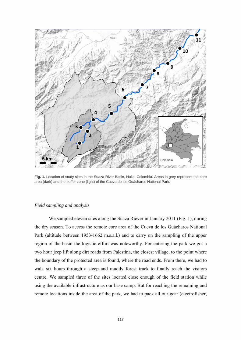
117
Fig. 1. Location of study sites in the Suaza River Basin, Huila, Colombia. Areas in grey represent the core area (dark) and the buffer zone (light) of the Cueva de los Guácharos National Park.
Field sampling and analysis
We sampled eleven sites along the Suaza Riever in January 2011 (Fig. 1), during
the dry season. To access the remote core area of the Cueva de los Guácharos National
Park (altitude between 1953-1662 m.s.a.l.) and to carry on the sampling of the upper
region of the basin the logistic effort was noteworthy. For entering the park we got a
two hour jeep lift along dirt roads from Palestina, the closest village, to the point where
the boundary of the protected area is found, where the road ends. From there, we had to
walk six hours through a steep and muddy forest track to finally reach the visitors
centre. We sampled three of the sites located close enough of the field station while
using the available infrastructure as our base camp. But for reaching the remaining and
remote locations inside the area of the park, we had to pack all our gear (electrofisher,
118
waders, multiparametrics, some supplies etc.) and walk for two days through the jungle
guided by an experienced park ranger.
At each sampling site, conductivity (µS/cm), water temperature (°C), dissolved
oxygen (mg l-1) and pH were measured in situ with a multi-parameter probe (Hanna
Instrument, HI 98129 Combo Waterproof). As indicators of water pollution and with
the aim to assess water quality, samples were collected and analysed for ammonium
(NH4+, mg L-1), orthophosphate (PO43-, mg L-1), nitrite (NO2-, mg L-1), and nitrate (NO3-
, mg L-1) using standard methods (APHA et al., 1992).
Characterization of habitat structure was done using transects according to
Armantrout (1998), and included depth (m), width (m), water velocity (m·s-1), percent
tree canopy shading and dominant substrate categorized as fines (<2 mm), gravels (~2–
64 mm), pebbles (~64–256 mm), boulders (>256 mm), or bedrock and concrete.
Additionally, three habitat quality indices were measured: the Qualitative Habitat
Evaluation Index QHEI (Rankin, 1989), the Andean-adapted versions of the Fluvial
Habitat Index (Indice de Habitat Fluvial, or IHF) and the riparian forest quality index
QBR (Acosta et al., 2009) (Table 1). QHEI jointly considers different habitat
parameters, such as bottom substrate and embeddedness, instream structure, velocity
and depth regime, canopy cover, channel alteration and pool/riffle or run/bend ratios.
The IHF characterises the physical habitat of streams and rivers and evaluates the
relationship between habitat heterogeneity and the physical variables of the stream
channel. QBR index includes aspects of the riparian forest such as total riparian
vegetation cover, cover structure, cover quality and channel alterations.
Fish assemblages were sampled in January 2011, in the dry season, following a
standardized protocol. Length of stream sampled was typically around 100 m and
covered all habitat types in the vicinity (e.g., riffles, runs and pools). Fish sampling was
taken by electrofishing surveys (Hans Grassl model IG200/2D, 300-600V, 0.2–2A)
following a single-run depletion methodology and estimating fish abundance. Semi-
quantitative surveys with a constant unit of effort (30 minutes per survey) were
conducted (Meador et al. 2003), yielding fish densities by catch per unit effort (CPUE,
number of specimens collected per hour). Collected fish were anesthetized with 2-
phenoxyethanol (0.1-0.2 mg l-1) and subsequently counted, measured and released after
119
the survey. For each individual, total length (TL) was measured to the nearest 0.01 cm,
and whole body weight (W) was taken on a digital balance with 0.05 g accuracy.
Voucher specimens of each species were euthanatized and taken to the
laboratory, fish were preserved in alcohol (75%) and identified to species, when
possible, or to higher taxonomic levels (i.e., genus or family) when taxonomic
information was insufficient for a reliable identification. Fish were identified using
taxonomic keys and other published literature (Mojica et al. 2005, Galvis et al. 2006,
Maldonado-Ocampo et al. 2008, Gaspar et al. 2012) as well as the collaborative efforts
of J. I. Mojica (Universidad Nacional de Colombia, Bogotá, D.C., Colombia), F.
Provenzano (Universidad Central de Venezuela, Caracas, Venezuela) and J. A.
Maldonado-Ocampo (Pontificia Universidad Javeriana, Bogotá, D.C., Colombia). Most
species have complex taxonomic relationships that are unclear at present, and
researchers are not in full agreement on their taxonomic status. For this reason, the
nomenclatural assignments of Eschmeyer et al. (2016) were used.
Macroinvertebrate sampling was conducted for evaluating water quality and
applying the BMWP procedure (Biological Monitoring Working Party) (Armitage et al.
1983). The BMWP is a procedure for measuring water quality using macroinvertebrates
as biological indicators. A hand-net (25 cm x 25 cm aperture, 100-µm-mesh size) was
used for the collection. Samples were preserved in 5% buffered formaldehyde for later
identification in the laboratory. Specimens were identified to the family level and the
adapted BMWP index for Andean rivers developed to Colombia (BMWP/Col) was
applied (Roldán 2003), obtaining water quality values for all sampling sites.
Data analysis
From fish community compositional data, richness (Margalef’s index R = (S-1)/
ln N), diversity (Shannon–Wiener index H’=-∑pi log2pi) and dominance (Simpson’s
index D = ∑pi2) measures were calculated, where pi is the proportion of species «i» at a
given site and S is the number of species (Margalef, 1980). Besides, Bray-Curtis index
of similarity was used to compare fish assemblages between study sites. A matrix of
abundances was used for studying fish community clustering using PAST statistical
software (Hammer et al. 2001; Table 2). This analysis provides a different approach for
studying the potential habitat distribution inferred from the similarity and grouping of
120
sites and highlights different habitat ranges exclusively related to the faunistic
assemblages.
We studied the association between the diversity and relative abundance of
fishes and the environmental variables of sampling points using Canonical
Correspondence Analyses (CCA). The main result is a scatterplot ordination diagram
displaying the pattern of fish assemblage variation along the environmental variables
shown as vectors. Vector direction and length indicate the relative magnitude and
influence of a particular variable on fish assemblages. To reduce the influence of rare
species on the multivariate analyses, poorly represented species (occurring in only one
site) were removed from this analysis, and taxa were grouped by genus. The
significance of the analyses was assessed by a permutation test with 999 random
permutations.
A CCA was used on a matrix of the relative abundance of species by site (Table
2) to evaluate the distribution of fish species among study sites and their relationship
with natural habitat characteristics, related to depth, width, canopy cover, water velocity
and substrate of riverbed. The percentage of bedrock and concrete (poorly represented)
was eliminated to avoid problems of multicollinearity among substrate predictor
variables. A second CCA analysis was applied to evaluate the distribution of fish among
study sites and their relationship with environmental quality. We used a matrix of
relative abundances of fish families and a matrix of environmental quality including
concentrations of potential water pollution indicators (nitrite, nitrate, ammonium, and
orthophosphate), hydrochemical parameters (temperature, conductivity, pH, and
dissolved oxygen), and scores of environmental quality indices (IHF, QBR, QHEI, and
RBMWP/ Col; Table 1).
To improve linearity, environmental data were transformed by using ln (x + 1).
Particularly for percentage data, logit-transformation was used, since Warton and Hui
(2011) recommend this method to analyse proportions in ecology research, as an
alternative to arcsine square root transformation. Abundance fish data were root
transformed. Assumptions of normality of distributions and homogeneity of variances
were verified through Shapiro-Wilks and Levene’s tests, respectively. The significance
level was set at P-value = 0.05. The statistical analyses were conducted with PAST
(v2.17) statistical software ((Hammer et al. 2001).
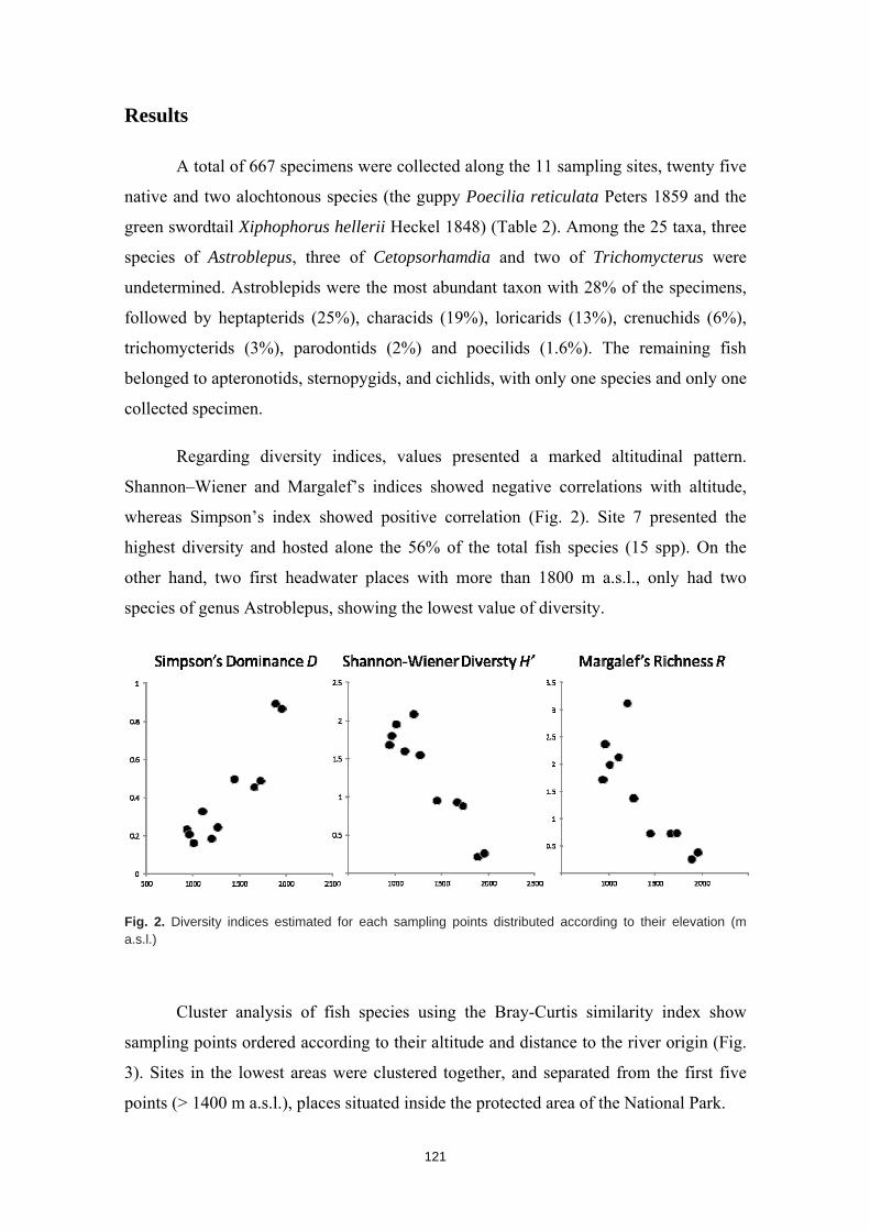
121
Results
A total of 667 specimens were collected along the 11 sampling sites, twenty five
native and two alochtonous species (the guppy Poecilia reticulata Peters 1859 and the
green swordtail Xiphophorus hellerii Heckel 1848) (Table 2). Among the 25 taxa, three
species of Astroblepus, three of Cetopsorhamdia and two of Trichomycterus were
undetermined. Astroblepids were the most abundant taxon with 28% of the specimens,
followed by heptapterids (25%), characids (19%), loricarids (13%), crenuchids (6%),
trichomycterids (3%), parodontids (2%) and poecilids (1.6%). The remaining fish
belonged to apteronotids, sternopygids, and cichlids, with only one species and only one
collected specimen.
Regarding diversity indices, values presented a marked altitudinal pattern.
Shannon–Wiener and Margalef’s indices showed negative correlations with altitude,
whereas Simpson’s index showed positive correlation (Fig. 2). Site 7 presented the
highest diversity and hosted alone the 56% of the total fish species (15 spp). On the
other hand, two first headwater places with more than 1800 m a.s.l., only had two
species of genus Astroblepus, showing the lowest value of diversity.
Fig. 2. Diversity indices estimated for each sampling points distributed according to their elevation (m a.s.l.)
Cluster analysis of fish species using the Bray-Curtis similarity index show
sampling points ordered according to their altitude and distance to the river origin (Fig.
3). Sites in the lowest areas were clustered together, and separated from the first five
points (> 1400 m a.s.l.), places situated inside the protected area of the National Park.
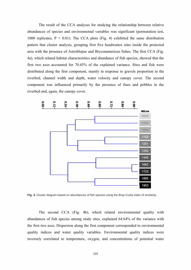
122
The result of the CCA analyses for studying the relationship between relative
abundances of species and environmental variables was significant (permutation test,
1000 replicates, P < 0.01). The CCA plots (Fig. 4) exhibited the same distribution
pattern that cluster analysis, grouping first five headwaters sites inside the protected
area with the presence of Astroblepus and Bryconamericus fishes. The first CCA (Fig.
4a), which related habitat characteristics and abundance of fish species, showed that the
first two axes accounted for 70.45% of the explained variance. Sites and fish were
distributed along the first component, mainly in response to gravels proportion in the
riverbed, channel width and depth, water velocity and canopy cover. The second
component was influenced primarily by the presence of fines and pebbles in the
riverbed and, again, the canopy cover.
Fig. 3. Cluster diagram based on abundances of fish species using the Bray-Curtis index of similarity.
The second CCA (Fig. 4b), which related environmental quality with
abundances of fish species among study sites, explained 64.64% of the variance with
the first two axes. Dispersion along the first component corresponded to environmental
quality indices and water quality variables. Environmental quality indices were
inversely correlated to temperature, oxygen, and concentrations of potential water
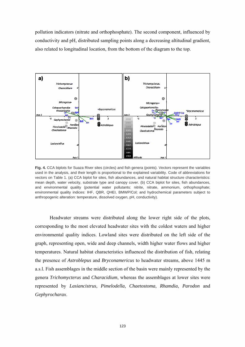
123
pollution indicators (nitrate and orthophosphate). The second component, influenced by
conductivity and pH, distributed sampling points along a decreasing altitudinal gradient,
also related to longitudinal location, from the bottom of the diagram to the top.
Fig. 4. CCA biplots for Suaza River sites (circles) and fish genera (points). Vectors represent the variables used in the analysis, and their length is proportional to the explained variability. Code of abbreviations for vectors on Table 1. (a) CCA biplot for sites, fish abundances, and natural habitat structure characteristics: mean depth, water velocity, substrate type and canopy cover. (b) CCA biplot for sites, fish abundances, and environmental quality (potential water pollutants: nitrite, nitrate, ammonium, orthophosphate; environmental quality indices: IHF, QBR, QHEI, BMWP/Col; and hydrochemical parameters subject to anthropogenic alteration: temperature, dissolved oxygen, pH, conductivity).
Headwater streams were distributed along the lower right side of the plots,
corresponding to the most elevated headwater sites with the coldest waters and higher
environmental quality indices. Lowland sites were distributed on the left side of the
graph, representing open, wide and deep channels, width higher water flows and higher
temperatures. Natural habitat characteristics influenced the distribution of fish, relating
the presence of Astroblepus and Bryconamericus to headwater streams, above 1445 m
a.s.l. Fish assemblages in the middle section of the basin were mainly represented by the
genera Trichomycterus and Characidium, whereas the assemblages at lower sites were
represented by Lasiancistrus, Pimelodella, Chaetostoma, Rhamdia, Parodon and
Gephyrocharax.
124
Discussion
Two distinct regions were identified in the Suaza River Basin as a result of the
observed environmental gradients and fish distribution: the upper region above 1400 m
a.s.l. and the lower region from 1400 m a.s.l. to its confluence with the Magdalena
River. The upper region, comprising the Cueva de los Guácharos National Park, is
characterized by the primary forest with steep slopes, deep valleys and gorges, and
pristine streams.
Downstream the sixth sampling point at 1280 m a.s.l., just in the limits of buffer
zone of the protected area (Fig. 1), the landscape change is remarkable. The slope
decreases and the river opens to a wider basin, followed by the appearance of the first
human settlements. Downstream this site the basin is extensively deforested. The slash-
and-burn technique has been widely used for obtaining land for agriculture and mainly
for cattle-raising. The exploitation of quinine in the 19th century and the involvement of
several companies in the Suaza River were responsible of the significant decrease of the
floral biodiversity of the valley (Sesana, 2006).
Changes in the valley morphology directly influence the structure and
composition of fish assemblages in terms of morphology and habitat use (Jaramillo-
Villa et al. 2010). Fishes show noticeable morphological and physiological adaptations
for survival in tropical Andean rivers (Anderson and Maldonado-Ocampo, 2010), and
changes of habitat characteristics an environmental quality levels modify severely the
fish abundance and distribution. The fish species diversity increased at lower altitudes
of the Suaza River, when slope decreased and temperature increased, primary
productivity increases and the river becomes more suitable for a wider range of species
(Pouilly et al., 2006).
At the highest localities in the basin, climbing catfishes (Astroblepus) were
found to be strongly and exclusively related to the headwaters, indicating turbulent, cold
streams that remain almost pristine. Climbing catfishes occur in streams across a wide
range of ecosystems from Panama to Bolivia, with most occurrences between 500 and
2000 m a.s.l. and associated principally with headwaters (Jaramillo-Villa et al., 2010).
Genus Bryconamericus appeared in higher elevations, close to Astroblepus populations,
associated with both lentic and lotic environments (Anderson and Maldonado-Ocampo,
125
2011), and related to clean waters and substrate composed to gravels and stones
(Román-Valencia 2003). Similar altitudes and environmental features were found for
other Bryconamericus populations (Román-Valencia and Muñoz, 2001; Valencia et al.,
2008). However, this genus appears often related to low elevation streams (~300 m
a.s.l.), wide stretches, high temperature and smooth slopes in a contiguous basin in the
Andean-Amazonian piedmont (Tobes et al., 2016).
Regarding to Trichomycterus and Characidium, these genera are related to
shallow and turbulent waters and substrates with gravels, fines and pebbles, although
they can be present in a wide range of river habitats (Maldonado-Ocampo et al. 2005).
Fishes related to lowland places of Suaza River (Lasiancistrus, Chaetosotma, Rhamdia,
Pimelodella and Parodon) are related to the medium stretches of rivers with rocky
substrates and torrent waters (Fialho et al., 2008; Tobes et al. 2016).
The presence of two exotic fishes (Poecilia reticulata and Xiphophorus helleri)
is an alarming discovery. Both species have been widely introduced in all continents
(ISSG, 2015) and their impact over other native fishes has been extensively studied (e.g.
Courtenay and Meffe, 1989). These species are popular aquarium species and their
presence in the Suaza River may be the result of escapes or releases from aquaria
(Gozlan et al. 2010). It is mandatory to manage and eradicate these populations because
of the major treat they represent for native fauna.
From the 27 studied species, only one species (Bryconamericus huilae) has been
evaluated and included in the IUCN Red List of Threatened Species as “least concern”
(IUCN, 2015). Four of the collected fish species (Bryconamericus huilae, Creagrutus
magdalenae, Chaetostoma thomsoni and Cynodonichthys magdalenae) are endemic of
Magdalena Basin, and the present study reports the first occurrences of these species in
the upper Magdalena. Regarding the knowledge of freshwater fishes in this area, it is
incipient, with some speies recently described (namely Bryconamericus huilae; Román-
Valencia, 2003), a genus recently revised as Lasiancistrus (Armbruster, 2005) or
Cynodonichthys (Costa, 2011), or species recently recognized as Rhamdia
guatemalensis, considered to date a synonymy of Rhamdia quelen in the northern South
America (Hernández et al., 2015). In the matter of the biology of these freshwater
fishes, in many cases only the environmental data included on the description of new
species are known, leaving an enormous knowledge gap concerning ecological
126
information. Because many rivers have never been inventoried, tropical Andean fishes
remain among the least studied and described vertebrates on the world (Jacobsen 2008).
The tropical Andes hotspot is considered as the most diverse biodiversity hotspot
in the world regarding its richness and endemism (Myers et al. 200). Unfortunately, our
lack of knowledge is very high about its biodiversity, and this void is especially
significant for freshwater fishes. However, this poor knowledge is due to a complex
reality that does not reflect scientific negligence (Arbeláez-Cortés, 2013). The access to
remote areas is not only difficult because of the complex logistics, it is also a dangerous
task. These faraway territories have been historically used as hiding places for many
outlaw organizations, as the FARC guerrilla or the paramilitary groups in Colombia.
They are frequently used for coca and opium plantations and certain areas are sowed
with anti-personnel mines (Thoumi, 2002). Therefore, sampling biodiversity in these
remote locations becomes an adventurous and risky duty and represents an major
impediment for science. However, there is a bright side, these dangerous territories are
avoided not only by scientist but also for any other kind of land uses, so the “restriction”
guarantees conservation. Nevertheless, there is an urgent priority to change the current
scenario, with the aim to improve our knowledge of Colombian biodiversity, “a unique,
irreplaceable, and very important natural resource of the country”, according to
Arbeláez-Cortés (2013).
Besides, many remote places of Andes are seriously threatened for current and
future exploitation projects (Finer et al. 2008, Finer and Jenkins 2012). These projects
will impact specially rivers and water resources, so future efforts should be focused on
the study of freshwater fishes of this singular region before it turns too late. Before we
lose unique biodiversity we haven’t even met.
127
Acknowledgments
The authors are grateful to the Aljemiro Escobar, Darwin Lenin Morabowen and
Kevin Usnavy Osorio for their invaluable field assistance and friendship. We thank the
collaborative efforts of J. I. Mojica (Universidad Nacional de Colombia, Bogotá, D.C.,
Colombia), F. Provenzano (Universidad Central de Venezuela, Caracas, Venezuela) and
J. A. Maldonado-Ocampo (Pontificia Universidad Javeriana, Bogotá, D.C., Colombia)
for assistance to identification of species. The authors are grateful to the Asociación de
Amigos – University of Navarra, which awarded Ibon Tobes a doctoral grant (2012-
2014). Vice-rectory of Research of the Universidad de la Amazonia provided logistic
and economics resources for the achievement of this work.
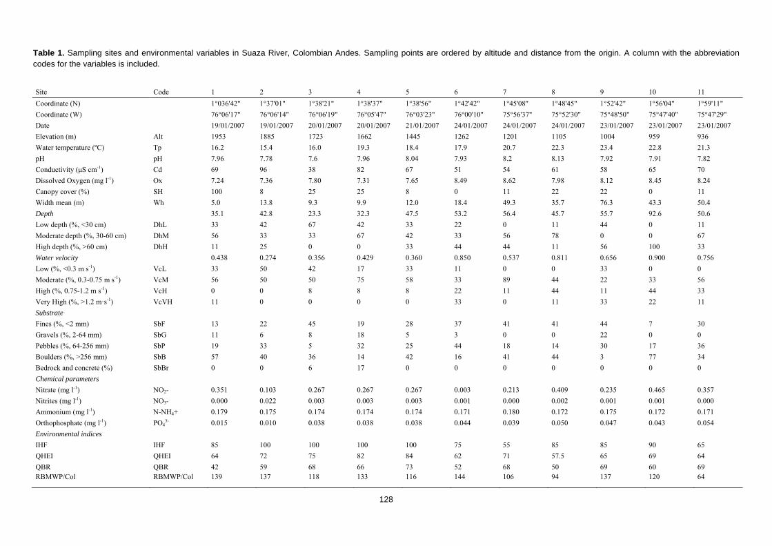
128
Table 1. Sampling sites and environmental variables in Suaza River, Colombian Andes. Sampling points are ordered by altitude and distance from the origin. A column with the abbreviation codes for the variables is included.
Site Code 1 2 3 4 5 6 7 8 9 10 11
Coordinate (N) 1°036'42" 1°37'01" 1°38'21" 1°38'37" 1°38'56" 1°42'42" 1°45'08" 1°48'45" 1°52'42" 1°56'04" 1°59'11"
Coordinate (W) 76°06'17" 76°06'14" 76°06'19" 76°05'47" 76°03'23" 76°00'10" 75°56'37" 75°52'30" 75°48'50" 75°47'40" 75°47'29"
Date 19/01/2007 19/01/2007 20/01/2007 20/01/2007 21/01/2007 24/01/2007 24/01/2007 24/01/2007 23/01/2007 23/01/2007 23/01/2007
Elevation (m) Alt 1953 1885 1723 1662 1445 1262 1201 1105 1004 959 936
Water temperature (ºC) Tp 16.2 15.4 16.0 19.3 18.4 17.9 20.7 22.3 23.4 22.8 21.3
pH pH 7.96 7.78 7.6 7.96 8.04 7.93 8.2 8.13 7.92 7.91 7.82
Conductivity (μS cm-1) Cd 69 96 38 82 67 51 54 61 58 65 70
Dissolved Oxygen (mg l-1) Ox 7.24 7.36 7.80 7.31 7.65 8.49 8.62 7.98 8.12 8.45 8.24
Canopy cover (%) SH 100 8 25 25 8 0 11 22 22 0 11
Width mean (m) Wh 5.0 13.8 9.3 9.9 12.0 18.4 49.3 35.7 76.3 43.3 50.4
Depth 35.1 42.8 23.3 32.3 47.5 53.2 56.4 45.7 55.7 92.6 50.6
Low depth (%, <30 cm) DhL 33 42 67 42 33 22 0 11 44 0 11
Moderate depth (%, 30-60 cm) DhM 56 33 33 67 42 33 56 78 0 0 67
High depth (%, >60 cm) DhH 11 25 0 0 33 44 44 11 56 100 33
Water velocity 0.438 0.274 0.356 0.429 0.360 0.850 0.537 0.811 0.656 0.900 0.756
Low (%, <0.3 m s-1) VcL 33 50 42 17 33 11 0 0 33 0 0
Moderate (%, 0.3-0.75 m s-1) VcM 56 50 50 75 58 33 89 44 22 33 56
High (%, 0.75-1.2 m s-1) VcH 0 0 8 8 8 22 11 44 11 44 33
Very High (%, >1.2 m·s-1) VcVH 11 0 0 0 0 33 0 11 33 22 11
Substrate
Fines (%, <2 mm) SbF 13 22 45 19 28 37 41 41 44 7 30
Gravels (%, 2-64 mm) SbG 11 6 8 18 5 3 0 0 22 0 0
Pebbles (%, 64-256 mm) SbP 19 33 5 32 25 44 18 14 30 17 36
Boulders (%, >256 mm) SbB 57 40 36 14 42 16 41 44 3 77 34
Bedrock and concrete (%) SbBr 0 0 6 17 0 0 0 0 0 0 0
Chemical parameters
Nitrate (mg l-1) NO2- 0.351 0.103 0.267 0.267 0.267 0.003 0.213 0.409 0.235 0.465 0.357
Nitrites (mg l-1) NO3- 0.000 0.022 0.003 0.003 0.003 0.001 0.000 0.002 0.001 0.001 0.000
Ammonium (mg l-1) N-NH4+ 0.179 0.175 0.174 0.174 0.174 0.171 0.180 0.172 0.175 0.172 0.171
Orthophosphate (mg l-1) PO43- 0.015 0.010 0.038 0.038 0.038 0.044 0.039 0.050 0.047 0.043 0.054
Environmental indices
IHF IHF 85 100 100 100 100 75 55 85 85 90 65
QHEI QHEI 64 72 75 82 84 62 71 57.5 65 69 64
QBR QBR 42 59 68 66 73 52 68 50 69 60 69 RBMWP/Col RBMWP/Col 139 137 118 133 116 144 106 94 137 120 64
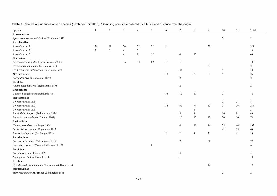
129
Table 2. Relative abundances of fish species (catch per unit effort). “Sampling points are ordered by altitude and distance from the origin.
Species 1 2 3 4 5 6 7 8 9 10 11 Total
Apteronotidae
Apteronotus rostratus (Meek & Hildebrand 1913) 2 2
Astroblepidae
Astroblepus sp.1 26 98 74 72 22 2 30 324
Astroblepus sp.2 2 6 4 2 14
Astroblepus sp.3 4 8 12 4 12 40
Characidae
Bryconamericus huilae Román-Valencia 2003 36 44 82 12 12 186
Creagrutus magdalenae Eigenmann 1913 2 2
Gephyrocharax melanocheir Eigenmann 1912 34 4 38
Microgenys sp. 14 2 6 4 26
Roeboides dayi (Steindachner 1878) 2 2
Cichlidae
Andinoacara latifrons (Steindachner 1878) 2 2
Crenuchidae
Characidium fasciatum Reinhardt 1867 58 12 10 2 82
Heptapteridae
Cetopsorhamdia sp.1 2 2 4
Cetopsorhamdia sp.2 38 62 74 12 2 26 214
Cetopsorhamdia sp.3 2 2
Pimelodella chagresi (Steindachner 1876) 8 8 16 8 40
Rhamdia guatemalensis (Günther 1864) 10 12 12 30 10 74
Loricariidae
Chaetostoma thomsoni Regan 1904 4 10 16 28 44 102
Lasiancistrus caucanus Eigenmann 1912 42 18 60
Rineloricaria jubata (Boulenger 1902) 2 2 4 2 6 16
Parodontidae
Parodon suborbitalis Valenciennes 1850 2 20 22
Saccodon dariensis (Meek & Hildebrand 1913) 6 6
Poeciliidae
Poecilia reticulata Peters 1859 4 4
Xiphophorus hellerii Heckel 1848 18 18
Rivulidae
Cynodonichthys magdalenae (Eigenmann & Henn 1916) 12 12
Sternopygidae
Sternopygus macrurus (Bloch & Schneider 1801) 2 2
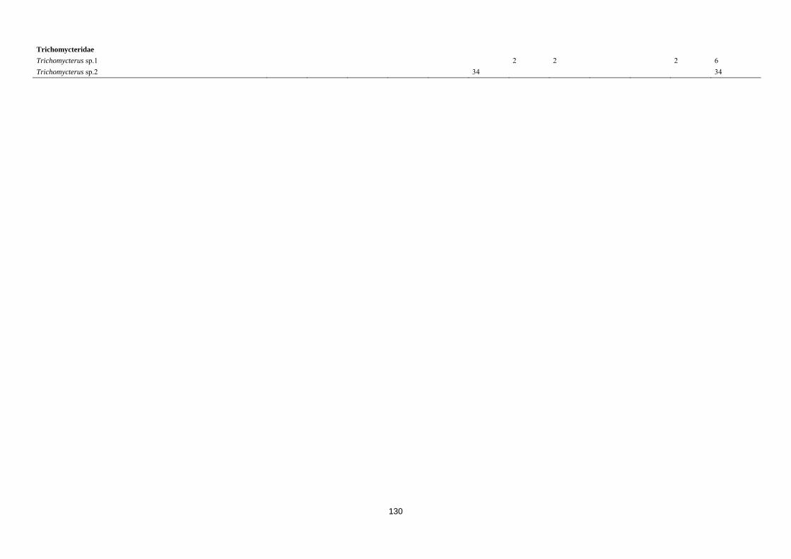
130
Trichomycteridae
Trichomycterus sp.1 2 2 2 6
Trichomycterus sp.2 34 34
131
CAPÍTULO 5TH CHAPTER RELACIONES BIOMÉTRICAS DE LOS PECES DEL RÍO SUAZA (DEPARTAMENTO DE HUILA, COLOMBIA) Biometric relationships of freshwater fishes of the Suaza River (Huila Department, Colombia)
Tobes I, Gaspar S, Peláez‐Rodríguez M, Miranda R
Enviado a Acta Ichthyologica et Piscatoria

132
133
Resumen
El conocimiento de peces de agua dulce en las remotas cabeceras de los Andes Tropicales es escaso y
se limita a examinar el cambio de la distribución de ocurrencia a lo largo de un gradiente específico.
El alto número de especies endémicas de peces requiere más estudios en cuanto a su biología y su
estado de conservación. Las relaciones talla-peso, longitud- y envergadura- longitud son útiles para
estimar la biomasa y las tallas de estos peces, y resulta una herramienta básica para su estudio. El
presente trabajo presenta las estimaciones de las relaciones morfométricas de nueve especies nativas
de peces de agua dulce (tres Loricariidae, dos Characidae, dos Heptapteridae, un Crenuchidae y un
Parodontidae) colectados en el río Suaza (Huila, Colombia). Estas son las primeras relaciones talla-
peso reportadas para todas estas especies, en su mayoría endémicas de los Andes colombianos. El
informe también proporciona el nuevo tamaño máximo de cuatro especies.
Palabras clave: longitud, peso, envergadura, peces neotropicales, ríos de montaña, Andes.
Abstract
Knowledge of freshwater fishes in the remote Andean mountains is scarce and restricted to examining
the change of occurrence distribution along a specific gradient. The high number of endemic fish
species requires further studies regarding their biology and their conservation status. The length-
weight, length-length and length- girth relationships are useful to estimate the biomass and lengths of
these fishes, and this is a basic tool for their study. The present work presents the estimates of
morphometric relationships for nine native freshwater fish species (three Loricariidae, two Characidae,
two Heptapteridae, one Crenuchidae and one Parodontidae) collected in the Suaza River (Huila,
Colombia). These are the first length-weight relationships reported for all these species, mostly
endemic to the Colombian Andes. The report also provides the new maximum size for four species.
Key words: length, weight, girth, Neotropical fishes, mountain river, Andes

Tobes I, Gaspar S, Peláez-Rodríguez M, Miranda R. Biometric relationships of freshwater fishes of the Suaza River (Huila Department, Colombia). Acta Ichthyologica et Piscatoria [under revision].

141
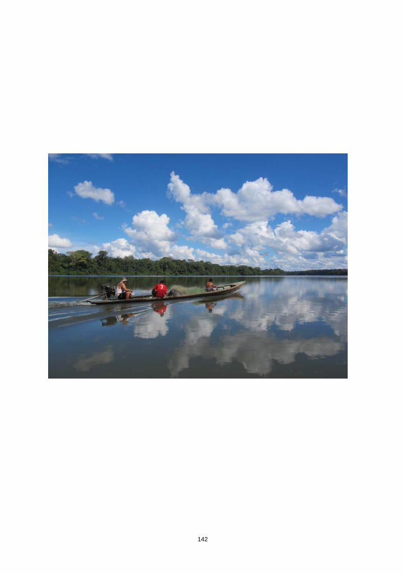
142
143
CAPÍTULO 6TH CHAPTER ECOLOGÍA Y PATRONES DE DISTRIBUCIÓN DE LAS COMUNIDADES DE PECES DEL RÍO ALTO MADRE DE DIOS, PERÚ: IMPLICACIONES DEL CONOCIMIENTO EN LA CONSERVACIÓN Y GESTIÓN Ecology and distribution patterns of fish assemblages in the Alto Madre de Dios River, Perú: implications of knowledge in the conservation and management Tobes I, Miranda R, Pino‐del‐Carpio A, Araujo‐Flores JM, Ortega H

144
145
Resumen
Este estudio analiza la ecología y la distribución espacial de las comunidades de peces relacionadas
con las variables ambientales del río Alto Madre de Dios. Los resultados presentados aportan nuevos
datos ecológicos de estos remotos ecosistemas de agua dulce apenas estudiados. El área de estudio se
encuentra entre los 300 y 2811 m, en el piedemonte amazónico de los Andes del Sur del Perú, dentro
de la Reserva de Biosfera del Manu. Mediante el uso de técnicas de electropesca se colectaron un
total de 1934 ejemplares de peces pertenecientes a 78 especies, 42 géneros y 15 familias. Los
carácidos fueron la familia más abundante sumando un 43% de las especies, seguidos por los
loricaridos (14%), trichomycteridos (8%), astroblepidos, cíclidos y heptapteridos (7% cada uno). La
riqueza de especies y la diversidad disminuyeron al aumentar la altitud, mientras que la dominancia
mostró un patrón inverso. Se llevaron a cabo análisis de correspondencias canónicas para obtener
una visión general de la estructura de las comunidades de peces en relación a los parámetros de
hábitats acuáticos. Así mismo, se aplicaron tres índices de calidad ambiental cuyos resultados
destacaron el buen estado de conservación de los ecosistemas estudiados. Sin embargo, la gran falta
de conocimiento en torno a la ecología de estos ríos y sus comunidades de peces supone un
importante obstáculo para el desarrollo de iniciativas de conservación y de gestión. Esta carencia
pone de manifiesto la urgente necesidad de nuevos estudios sistemáticos y ecológicos en torno a la
fauna de agua dulce de la región.
Palabras clave: Andes tropicales, índices de calidad ambiental, ríos neotropicales, dieta de los peces
146
Abstract
This study analyses the ecology and spatial distribution of fish assemblages related to environmental
variables of the Alto Madre de Dios River, contributing with new ecological data for these scarcely
studied and remote freshwater ecosystems. The study area is located between 300 and 2811 m.a.s.l. on
the Amazonian piedmont of the Southern Peruvian Andes, inside the Manu Biosphere Reserve. A total
of 1934 fish specimens belonging to 78 species, 42 genera and 15 families were collected using
electrofishing techniques. Characids were the most abundant taxon with 43% of the species, followed
by loricarids (14%), trichomycterids (8%), astroblepids, cichlids and heptapterids (7% each one).
Species richness and diversity declined rapidly with altitude, whereas dominance increased. Canonical
correspondence analyses were performed to obtain an overview of the fish community structure in
relation to aquatic habitat parameters. Some environmental quality indices were applied highlighting
the almost pristine conservation status of the streams. However, the great lack of knowledge
concerning freshwater ecology and fish communities represents an important restraint for conservation
and management initiatives, therefore systematic and ecological studies of the freshwater fish fauna of
this unique region are certainly needed.
Key words: Tropical Andes, environmental quality indices, neotropical stream, fish diet
147
Introduction
Freshwater ecosystems are often referenced among those that are most altered and
threatened by anthropogenic impacts (Gozlan, Britton, Cowx, & Copp, 2010) and their fauna
is at greater risk than any other animal and plant groups (Ricciardi & Rasmussen, 1999). The
decline in freshwater biodiversity is alarming and far greater than in the most affected
terrestrial ecosystems, positioning it as the over-riding conservation priority worldwide
(Dudgeon et al., 2006). In this respect, precise knowledge of ecological aspects like species
distribution and requirements are a key point for conservation strategies, especially when the
focal species are threatened or endangered (Dejean et al., 2011). Unfortunately, our limited
taxonomic knowledge and incomplete information on species distributions for broad
territories is very high, and represents an insurmountable obstacle for documentation of
imperilment and extinction of freshwater biodiversity (Allan & Flecker, 1993). In particular,
fish assemblage variations in mountain streams of the Andes are poorly understood, where
only few descriptive studies have been carried out (Barthem et al., 2003; Maldonado-Ocampo
et al., 2005; Lujan et al., 2013).
The tropical Andes is regarded as the richest of the 25 recognized global biodiversity
hotspots and its streams are ecologically important as the headwaters of the megadiverse
lowland river systems in South America (Albert & Reis, 2011). They are responsible of
delivering major loads of inorganic sediment and organic carbon to lowlands (Townsend-
Small et al., 2008) and play a key role in the ecological processes along the Andes-to-Amazon
fluvial continuum (Laraque et al., 2009). Furthermore, the Andean flank of the Amazon hosts
the highest biodiversity rates and has been least affected by historical climate variability and
land use (Malhi et al., 2008).
However, the Andean-Amazonian piedmont is a rapidly changing landscape, part of
the “arc of deforestation” (Aldrich et al., 2012), caused foremost by the expansion of cattle
and soybean production (Myers, 1993). The recent growth of human populations and the
exploitation of natural resources are leading to extensive reductions in habitats and
subsequent impacts on rivers (Brooks et al., 2002). Additionally, the proliferation of
hydroelectric dams in the Andean Amazon valleys represents a major threat for the integrity
of these ecosystems and may lead to irreversible and unpredictable changes both in the
148
headwaters and specially for the lowland areas in the Amazon (Finer & Jenkins, 2012).
Fortunately, many opportunities for protecting these habitats yet exist, particularly in Peru,
where entire river systems are still relatively intact and where there are few large dams and
other major structural changes to river channels (Nilsson et al., 2005).
Our study area, the Alto Madre de Dios River Basin, in the south west of Peru, is an
almost pristine basin. It’s located in the Andean-Amazonian piedmont, in the transition zone
of the Manu Biosphere Reserve, bordered on the northwest by the Manu National Park, and
on the southeast by the Amarakaeri Communal Reserve, two important protected areas of the
Peruvian Amazon. This region has long been known to tropical biologists as a region high in
species diversity, as well as some of the world’s largest expanses of pristine tropical forest
(Yu, Hendrickson & Castillo, 1997). Pitman et al. (Pitman et al., 2008) reviewed all the
scientific studies generated on the Department of Madre de Dios, and found that only 2.8% of
the analysed manuscripts focus on fish or hydrobiology. Just lichens have received less
attention than fish. Other research works regarding plants or mammals comprise 21.3% and
16.6% of the total scientific literature respectively.
However, Peru is home to 1,010 fish species (Ortega et al., 2010a), more than the 7%
of all the globally known freshwater species. Most of them (more than 800) are found in the
Amazonian Basin (Ortega & Hidalgo, 2008). Only during the past decade 155 new species
were named in Peru (Ortega et al., 2012) and the experts estimate the total number of
Peruvian freshwater fishes at approximately 1,200 spp. (Ortega & Chang, 1998). But as seen
before, there have been few ecological surveys focusing on fish and the majority point out the
uneven level of knowledge for this group of vertebrates (Ortega & Hidalgo, 2008), with some
taxa itemized at the species level, whereas others routinely are catalogued at family level,
order or even phylum (Allan & Flecker, 1993).
Given the pessimistic predictions for the sustainability and conservation of the Andean
biodiversity due to environmental alterations (Vuille et al., 2008; Jaramillo-Villa, Maldonado-
Ocampo & Escobar, 2010; Swenson e al., 2011) studies on the biotic and abiotic factors
conditioning the abundance and distribution of Andean fish are critical to document the
primary characteristics of the original communities and thereby contribute to the delimitation
of appropriate conservation areas and/or to recovery strategies. Furthermore, Andean rivers
are ecologically relevant as the upstream branches of the mega-diverse wetlands in the
149
Amazon plain, and freshwater fish should be considered as fundamental indicators of
ecological conditions in these critical regions (Finer & Jenkins, 2012).
In the present study we examine the freshwater ecology for the Alto Madre de Dios
River focusing on its ichthyofauna and to evaluate the environmental integrity of the studied
ecosystems. Our specific objectives are to (1) describe spatial variation of fish assemblage of
an unstudied Andean-Amazonian stream, and (2) to identify patterns of association between
fish assemblages and habitat variables.
Materials and methods
Study area
The Manu National Park has been considered one of the world’s most important
tropical protected areas since its creation in 1973 (Shepard et al., 2010). It is located in the
southern Peruvian Amazon rainforest and constitutes the core of the Manu Biosphere Reserve
and an IUCN World Heritage Site (Salvador, Clavero & Pitman, 2011). The southern buffer
zone of Manu Biosphere Reserve includes the Alto Madre de Dios basin (11°00’-13°30’S,
73°30’-68°30’W) (Fig. 1). The river flows, south to north, for 275 km through the rainforest
of Cusco and Madre de Dios Departments, draining an area of approximately 1600 km2. The
altitude in the basin varies from up to 3500 to 300 m.a.s.l. in the Manu River junction,
spanning five Andean vegetation zones: puna (4500–3500 m), upper cloud forest (3500–2500
m), lower cloud forest (2500–1000 m), piedmont (1000–400 m) and lowlands (400–50 m)
(Brack & Mendiola, 2000). Our highest sampling site was located at 2411 m.a.s.l. while to
lowest was at 398 m.a.s.l., 80 kms downstream. Rivers flow through deep and narrow valleys
and steep slopes from the source to around 700 m.a.s.l., where the valleys open to wide and
flat lowland floodplains. Flow regime is highly responsive to rainfall, and presents the
greatest discharge period from November to April, decreasing progressively in the dry season
(from May to October). The rivers remain turbid through the year, with highest sediment
loads during the rainy season.
Population density in the Alto Madre de Dios valley is low, with scattered settlements
which are under the administration of the village of Pilcopata in the District of Kosñipata,
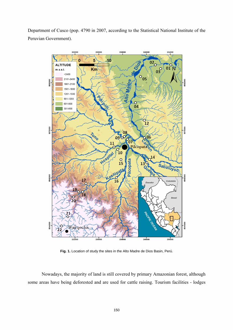
150
Department of Cusco (pop. 4790 in 2007, according to the Statistical National Institute of the
Peruvian Government).
Fig. 1. Location of study the sites in the Alto Madre de Dios Basin, Perú.
Nowadays, the majority of land is still covered by primary Amazonian forest, although
some areas have being deforested and are used for cattle raising. Tourism facilities - lodges
151
and a network of forest trails - are used by a relatively low number of tourists in comparison
with other lodges in Madre de Dios area (Yu, Hendrickson & Castillo, 1997).
Field sampling and analysis
Our survey was conducted at twenty-two sampling sites in June 2012 (Fig. 1). The
following environmental variables were recorded at each site using a multiparametric probe
(Hanna Instrument, HI 98129 Combo Waterproof): conductivity (µS/cm), water temperature
(°C), and pH. Characterization of habitat structure was done using transects according to
Armantrout (1998), and included depth (m), width (m), water velocity (m·s-1), percent tree
canopy shading and dominant substrate categorized as fines (<2 mm), gravels (~2–64 mm),
pebbles (~64–256 mm), boulders (>256 mm), or bedrock and concrete. Additionally, two
habitat quality indices were measured: the Qualitative Habitat Evaluation Index QHEI
(Rankin, 1989), and the Andean adapted version of the riparian forest quality index QBR
(Acosta et al., 2009) (Table 1). QHEI jointly considers different habitat parameters, such as
bottom substrate and embeddedness, instream structure, velocity and depth regime, canopy
cover, channel alteration and pool/riffle or run/bend ratios. QBR index includes aspects of the
riparian forest such as total riparian vegetation cover, cover structure, cover quality and
channel alterations.
Fish sampling was carried out by electrofishing surveys, using a backpack
electrofishing gear (Hans Grassl model IG200/2D, 300-600V, 0.2-2A) following a single-run
depletion methodology and estimating fish abundance based on catch per unit effort (CPUE)
(Meador, McIntyre & Pollock, 2003). Collected fish were anesthetized and subsequently
counted, measured to the nearest 0.1 cm total length (TL), weighed with a digital scale to an
accuracy of 0.05 g, and released after the survey, with the exception of some voucher
specimens kept for posterior identification.
Voucher specimens were deposited in the fish collection of the Natural History
Museum of National University of San Marcos (Lima, Peru). In the laboratory, fish were
preserved in alcohol (75%) and identified by Ana María Cortijo, Jessica Espino and Hernán
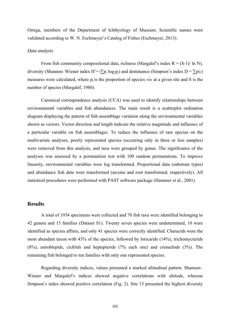
152
Ortega, members of the Department of Ichthyology of Museum. Scientific names were
validated according to W. N. Eschmeyer’s Catalog of Fishes (Eschmeyer, 2013).
Data analysis
From fish community compositional data, richness (Margalef’s index R = (S-1)/ ln N),
diversity (Shannon–Wiener index H’=-∑pi log2pi) and dominance (Simpson’s index D = ∑pi2)
measures were calculated, where pi is the proportion of species «i» at a given site and S is the
number of species (Margalef, 1980).
Canonical correspondence analysis (CCA) was used to identify relationships between
environmental variables and fish abundances. The main result is a scatterplot ordination
diagram displaying the pattern of fish assemblage variation along the environmental variables
shown as vectors. Vector direction and length indicate the relative magnitude and influence of
a particular variable on fish assemblages. To reduce the influence of rare species on the
multivariate analyses, poorly represented species (occurring only in three or less samples)
were removed from this analysis, and taxa were grouped by genus. The significance of the
analyses was assessed by a permutation test with 100 random permutations. To improve
linearity, environmental variables were log transformed. Proportional data (substrate types)
and abundance fish data were transformed (arcsine and root transformed, respectively). All
statistical procedures were performed with PAST software package (Hammer et al., 2001).
Results
A total of 1934 specimens were collected and 78 fish taxa were identified belonging to
42 genera and 15 families (Dataset S1). Twenty seven species were undetermined, 10 were
identified as species affinis, and only 41 species were correctly identified. Characids were the
most abundant taxon with 43% of the species, followed by loricarids (14%), trichomycterids
(8%), astroblepids, cichlids and heptapterids (7% each one) and crenuchids (3%). The
remaining fish belonged to ten families with only one represented species.
Regarding diversity indices, values presented a marked altitudinal pattern. Shannon–
Wiener and Margalef’s indices showed negative correlations with altitude, whereas
Simpson’s index showed positive correlation (Fig. 2). Site 13 presented the highest diversity
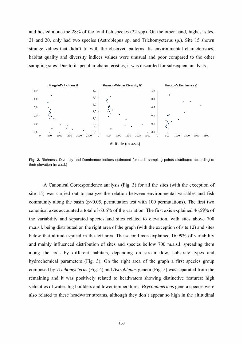
153
and hosted alone the 28% of the total fish species (22 spp). On the other hand, highest sites,
21 and 20, only had two species (Astroblepus sp. and Trichomycterus sp.). Site 15 shown
strange values that didn’t fit with the observed patterns. Its environmental characteristics,
habitat quality and diversity indices values were unusual and poor compared to the other
sampling sites. Due to its peculiar characteristics, it was discarded for subsequent analysis.
Fig. 2. Richness, Diversity and Dominance indices estimated for each sampling points distributed according to their elevation (m a.s.l.)
A Canonical Correspondence analysis (Fig. 3) for all the sites (with the exception of
site 15) was carried out to analyze the relation between environmental variables and fish
community along the basin (p<0.05, permutation test with 100 permutations). The first two
canonical axes accounted a total of 63.6% of the variation. The first axis explained 46,59% of
the variability and separated species and sites related to elevation, with sites above 700
m.a.s.l. being distributed on the right area of the graph (with the exception of site 12) and sites
below that altitude spread in the left area. The second axis explained 16.99% of variability
and mainly influenced distribution of sites and species bellow 700 m.a.s.l. spreading them
along the axis by different habitats, depending on stream-flow, substrate types and
hydrochemical parameters (Fig. 3). On the right area of the graph a first species group
composed by Trichomycterus (Fig. 4) and Astroblepus genera (Fig. 5) was separated from the
remaining and it was positively related to headwaters showing distinctive features: high
velocities of water, big boulders and lower temperatures. Bryconamericus genera species were
also related to these headwater streams, although they don´t appear so high in the altitudinal
154
gradient. A second group of fish composed by Astyanax, Corydoras, Knodus and Creagutus
genera, located on the bottom-left area of the graph, was positively related to still waters with
low velocities, higher conductivities and fine substrates (mainly sands). A third cluster,
located on the top-left area of the graph, included Hemibrycon, Hoplias, Chaetostoma and
Rineloricaria; related to open places with wide riverbed and mainly pebbles in the substrate.
Finally, on the central area of the diagram the rest of the genera and sites were gathered
together.
Fig. 3. CCA biplots for sites (squares) and fish genera (points). Vectors represent the variables used in the
analysis, and their length is proportional to the explained variability.
Attending to fish distribution and trophic specialization along the altitudinal gradient
(Fig. 6), no fish were found above 2200 m.a.s.l. Astroblepus and Trichomycterus genus were
the only genus found on highest reaches, feeding exclusively on invertebrates, but even
155
though they appear tightly related to headwaters, they were found all along the basin with
occasional and scarce occurrence in lowland streams. At 1400 m three new genera appear;
one invertivorous Bryconamericus, and the first two hervibore-detritivores Chaetostoma and
Ancistrus genera. Above the 700 m other four invertiborous genera were found: Characidium,
Rhamdia, Creagrutus and Chasmocranus. The rest of the fish taxa were found below 622 m,
representing the majority of the diversity. The first piscivorous species were found at this
altitude.
Discussion
According to some ecological studies and inventories carried out in this area (Ortega,
Corahua & Palacios, 2006; Araújo-Flores, 2015), more than 130 species of freshwater fishes
have been reported in the Alto Madre de Dios. In the present study, only 78 species were
collected, due to two main reasons: (1) the limitations of the electrofishing technique and (2)
the location of the sampling sites, mainly distributed in the piedmont area.
Regarding electrofishing, only wadeable stretches were sampled, whereas bigger
courses or deep stretches were avoided. This limitation directed our sampling efforts to
smaller rivers and tributaries where the electrofisher gained efficiency (Allard et al., 2014).
Although this represents a significant impediment for carrying out a complete biological
survey, also brings up new opportunities. Most of the ichthyofaunal studies undertaken in
Amazonia have focused on the large rivers and commercially valuable species, therefore
small and none commercial fishes and secondary streams have been usually overlooked
(Mendonça et al., 2005). Guided by our limitations, part of our surveying efforts were
concentrated on this poorly studied ecosystems and species.
Besides the restrictions for choosing samplings sites, fish resistance to electrofishing
was significant. This resistance was favored by low water conductivity and temperature, high
velocities, shelter’s abundance or low visibility (Zalewski, 1985). Furthermore, capture
efficiency depended on the mobility of species: little benthic fish were collected easily, in
contrast to bigger well-swimmer species that escaped the electrofishers range. However,
according to other authors (Zalewski, 1985; Meador et al., 2003) electrofishing is the best
sampling method when your objectives are to estimate and quantify freshwater fish
156
populations in streams and wadeable rivers and to correlate these abundances with
environmental features, habitat characteristics, hydrochemical parameters or other ecological
measures. Besides, although electrofishing surveys have been widely achieved on the world,
they have been scarce in remote places like the Alto Madre de Dios Basin due to the more
complex logistics.
If we match our results with the survey carried out with seine nets by Araújo-Flores in
2013 (reported in Araújo-Flores, 2015) we find remarkable differences. Comparing the total
44 spp. reported by Araújo-Flores with our 78 spp. only 17 of them where captured by both
studies. Nevertheless, survey of Araújo-Flores focused on two rivers and its tributaries
(Pilcopata and Piñi-Piñi Rivers), distributing 10 sampling sites in a smaller area with a limited
altitudinal range (500-600 m.a.s.l.). If we compare our data for the three sites coinciding with
the survey of Araújo-Flores (sites 7, 8 and 9), although our sampling effort was lower (3 vs 10
sites) and our captured diversity smaller (26 vs 44 spp.), we collected 15 spp. missing in the
survey of Araújo-Flores. Therefore, although electrofishing is not as effective in tropical
streams as it is for temperate streams, it may be more effective for capturing some species that
seem to be underestimated by other techniques. Consequently, as we focused on understudied
small rivers and streams, catching poorly known small fish, using an uncommon technique for
tropical freshwaters, our study presents new and relevant taxonomic and ecological
information, providing data for some fish never captured before by previous surveys in the
area.
Concerning the diversity indices, a gradual increase in species richness and diversity is
expected along longitudinal gradients in lotic systems; associated with changes in resource
availability, channel morphology, flow regime and substrate type (Hoeinghaus, 2004;
Alexandre et al., 2010). Addition of species is usually related to an increase of habitats
motivated for the structural diversification of the environment downstream (Leunda et al.,
2012). Our study confirms this patter (Fig. 2), with the only exception of one sampling point
15, that doesn’t fit the trend due to its low diversity values, explained by its peculiar features
as seen later.
All the studied environmental variables were correspondent with the values reported
by other works for natural and unaltered streams of this territory (Jaramillo-Villa et al., 2010;
Schaefer & Arroyave, 2010; Lujan et al., 2013; Tobes et al., 2016). Quality indices of riparian
157
and fluvial habitat (QBR and QHEI) got very high scores in all the sampling points,
highlighting the good environmental quality, with some remarkable exceptions. Riparian
forest (and adjacent jungle) on the right bank of the sampling point 13, in the Queros River,
was inexistent due to deforestation for extensive cattle raising. Besides, sampling point 15
showed significant differences both in environmental and diversity features, as already
mentioned. This site belongs to a special type of aquatic ecosystem of Amazon forest, known
as Aguajal. They are backswamp forests, defined as forest on low-lying areas outside of
streams courses, usually dominated by palms (Mauritia flexuosa), although other tree species
like figs (Ficus spp.) can be abundant as well (Hamilton et al., 2007). They also tend to be
clear and acidic, in contrast to the higher turbidity and cirmuneutral pH of the streams around
(Goulding et al., 2003). Sampling point 15 presented the described characteristics and showed
low habitat quality indices (Table 1) and very low diversity of fishes (Fig. 2), with only three
species present: Moenkhausia oligolepis, Crenicichla semicincta and Hoplias malabaricus. In
particular, this Aguajal was confined by extensive cattle pastures surrounding it and was used
as drinking reservoir for cattle, showing a remarkable eutrophication. Because of its special
and no-comparable characteristics, this peculiar sampling point has been excluded for the
general comparative analysis.
Fish abundance and distribution in response to environmental variables was
represented using the CCA analysis (Fig. 3). The observed distribution of species along the
longitudinal gradient of the basin was comparable to other fish assemblages found in rivers
with similar characteristics in adjacent areas (Maldonado-Ocampo et al., 2005; Jaramillo-
Villa et al., 2010; Lujan et al., 2013; Tobes et al., 2016). This biotic zonation corresponds to
discontinuities in river geomorphology or abiotic conditions, and are usually related to
smooth transitions of abiotic factors contributing to nested patterns of assemblage
composition along the altitudinal gradient (Tejerina-Garro et al., 2005). The graph highlights
this zonation, distributing headwater sites and their fish assemblages on the right of the
diagram, related to fast running waters, boulders and low water temperatures, opposed to
lowland streams on the left of the graph related to fine substrates, higher water temperatures
and low velocities. The boundary between both zones is located at 700 m.a.s.l. when the basin
changes from the steep piedmont streams flowing through narrow valleys, to flat and wide
floodplains were river channels widen.
158
Genera Astroblepus and Trichomycterus co-occur in high reaches, being the unique
species present on the sites close to the sources. These genera are adapted to headwaters,
related to rocky substrates and cold, clean and well oxygenated water (Fig. 3). They are
benthonic species without scales and a powerful sucker mouth or opercular odontodes
(Schaefer & Arroyave, 2010) Nevertheless, they occasionally occur in lower areas, although
their distribution is usually limited to elevations greater than 400 m.a.s.l. (Lujan et al., 2013).
Bryconamericus, a rheophilic genus, is the next genus joining the headwater assemblage at
1400 m.a.s.l. (Fig. 6). They prefer areas of moderate to strong current and present even in the
torrential flows (Maldonado-Ocampo et al., 2005; Jaramillo-Villa et al., 2010), occupying
intermediate places between mountain upstream and jungle downstream. We also found some
Chaetostoma and Ancistrus fishes at this reaches, although they appeared closely related with
lower middle section streams (Fig. 3).
The shift in assemblage composition in response to geomorphological changes in the
basin is significant under the 700 m.a.s.l. We found the majority of the species related to these
lower reaches, distributed along the left area of the CCA (Fig. 3). Habitats with fine substrata,
very slow water velocities and more conductivity due to organic decomposition were related
with some characid genera (Astyanax, Knodus and Creagrutus) and genus Corydoras,
grouped on the bottom left area of the diagram (Fig. 3) (Aranha et al., 1998; Pouilly et al.,
2006). Other lotic places with a substrate dominated by pebbles and wide riverbed were
distributed on the top left of the diagram, related with Hemibrycon genera characids and
loricarids like Rineloricaria, Chaetostoma and Ancistrus (Barthem et al., 2003; Alexandre et
al., 2010; Goulding et al., 2003).
We also observed a remarkable zonation related to trophic niches (Fig. 6). Headwaters
were dominated exclusively by invertivorous Astroblepus (Fig. 5) and Trichomycterus (Fig.
4) fishes due to the scarcity of other food resources in these clean waters (Schaefer &
Arroyave, 2010). Although the first herbivore-detritivore Chaetostoma and Ancistrus
individuals were found starting at 1400 m.a.s.l., they got more abundant below 1000 m.a.s.l.,
once the river carries enough organic matter coming from the surrounding forest offering a
new trophic niche (Tobes et al., 2016). The first piscivorous species, Hoplias malabaricus and
Crenicichla semicincta, were distributed around 600 m.a.s.l. and below, first found at site 15,
the aguajal, where the Moenkhausia oligolepis community was very abundant providing
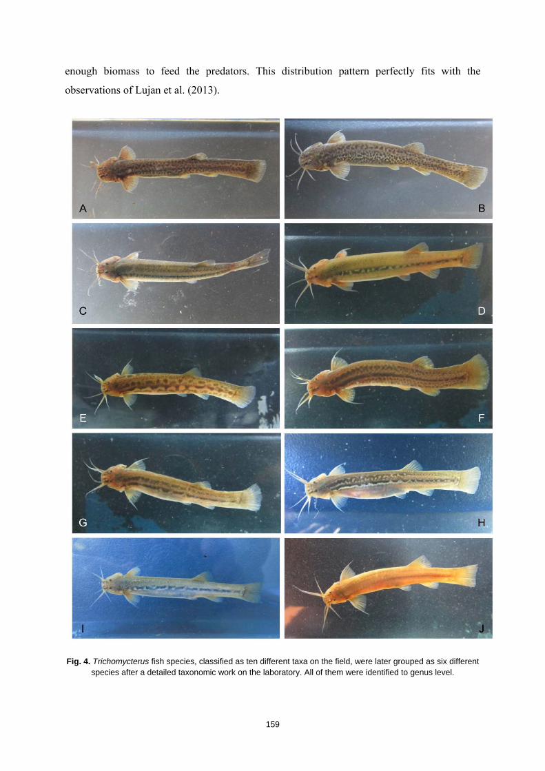
159
enough biomass to feed the predators. This distribution pattern perfectly fits with the
observations of Lujan et al. (2013).
Fig. 4. Trichomycterus fish species, classified as ten different taxa on the field, were later grouped as six different species after a detailed taxonomic work on the laboratory. All of them were identified to genus level.
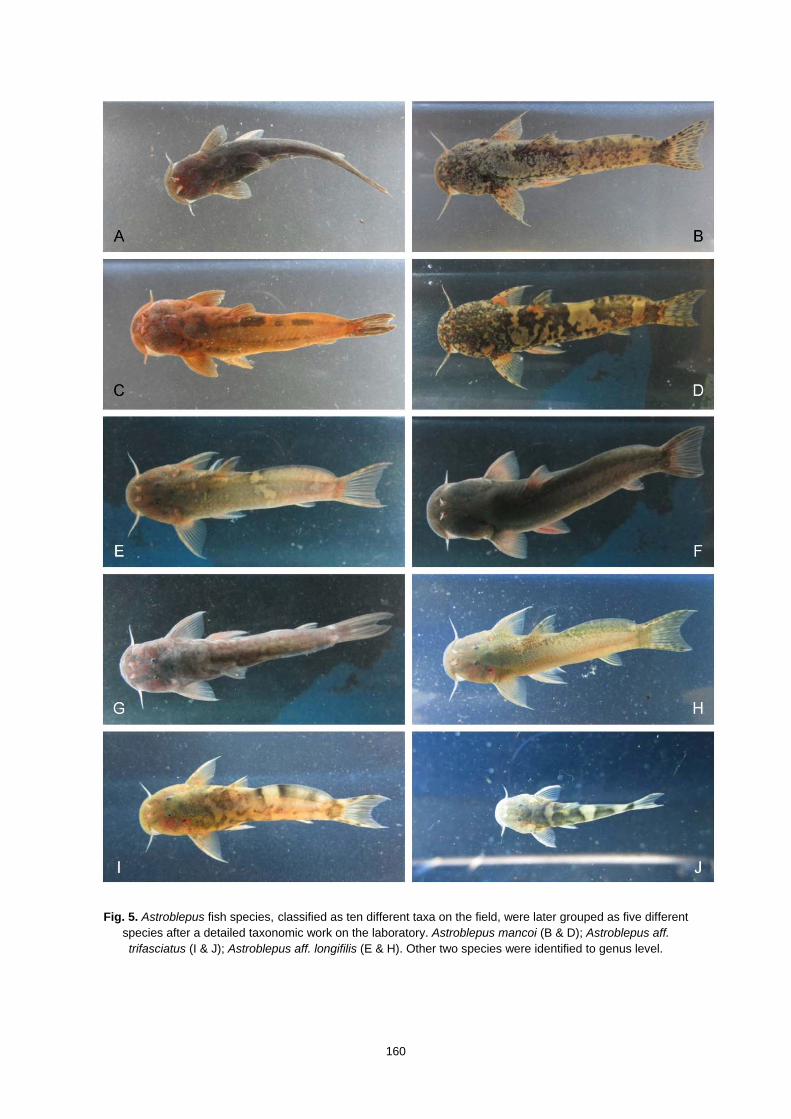
160
Fig. 5. Astroblepus fish species, classified as ten different taxa on the field, were later grouped as five different species after a detailed taxonomic work on the laboratory. Astroblepus mancoi (B & D); Astroblepus aff. trifasciatus (I & J); Astroblepus aff. longifilis (E & H). Other two species were identified to genus level.
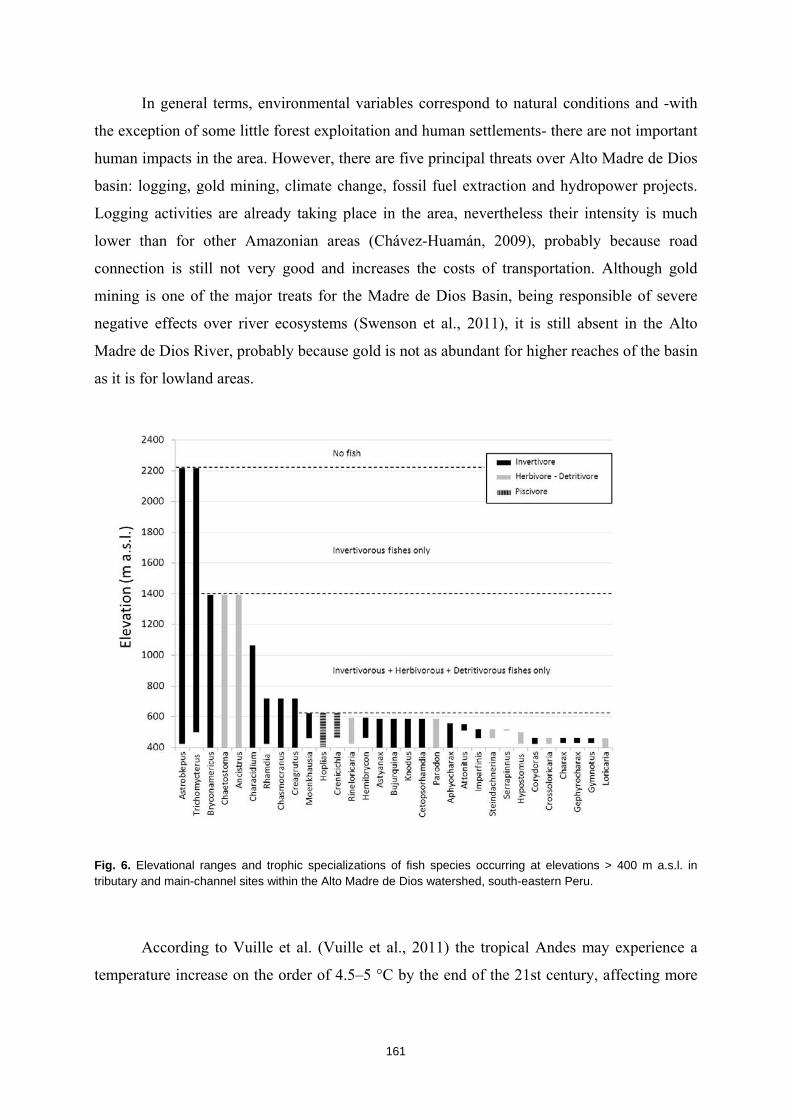
161
In general terms, environmental variables correspond to natural conditions and -with
the exception of some little forest exploitation and human settlements- there are not important
human impacts in the area. However, there are five principal threats over Alto Madre de Dios
basin: logging, gold mining, climate change, fossil fuel extraction and hydropower projects.
Logging activities are already taking place in the area, nevertheless their intensity is much
lower than for other Amazonian areas (Chávez-Huamán, 2009), probably because road
connection is still not very good and increases the costs of transportation. Although gold
mining is one of the major treats for the Madre de Dios Basin, being responsible of severe
negative effects over river ecosystems (Swenson et al., 2011), it is still absent in the Alto
Madre de Dios River, probably because gold is not as abundant for higher reaches of the basin
as it is for lowland areas.
Fig. 6. Elevational ranges and trophic specializations of fish species occurring at elevations > 400 m a.s.l. in tributary and main-channel sites within the Alto Madre de Dios watershed, south-eastern Peru.
According to Vuille et al. (Vuille et al., 2011) the tropical Andes may experience a
temperature increase on the order of 4.5–5 °C by the end of the 21st century, affecting more
162
severely high mountains than lower elevations (Bradley et al., 2006). Additionally, predicted
changes may cause an increase in precipitation during the wet season and a decrease during
the dry season, drastically modifying the seasonal hydrological cycle for the region (Vuille et
al., 2018).
The effects of this climate change, intensified by deforestation, would be catastrophic
for freshwater fauna, especially for the species with low mobility, strongly adapted to specific
seasonal changes. In addition, aquaculture is gaining importance as economic activity
especially along lower reaches of the basin (i.e. <400 m.a.s.l.) although it is still scarce in the
Alto Madre de Dios (Ortega & Hidalgo, 2008). However, the studied area presents a long-
lasting tradition of fish culture, and Pilcopata River has been catalogued with a high fish
production potential (Chávez-Huamán, 2009). Unfortunately, aquaculture of exotic species
(tilapias and carps) is promoted and growing in the Alto Madre de Dios, representing an
important threat to local diversity. Gas and oil extraction is responsible of critical
environmental impacts in the Amazon, caused by the construction of drilling platforms and
pipelines, and the contamination of rivers from oil spills and wastewater discharges (Finer et
al., 2008). Besides, it requires the creation of new roads that are responsible of several
indirect impacts like increase of human settlements, illegal colonization, logging, hunting and
wild meat trade (Suarez et al., 2009). One of the oil blocks under contract between Peruvian
government and a multinational company may be exploited in a near future inside the
Amarakaeri Communal Reserve, on the eastern Alto Madre de Dios River (Finer et al., 2008),
representing a major treat for the ecosystems and indigenous people in the area. Finally, there
proliferation of hydroelectric dams is threatening the integrity of many of the headwater
valleys draining the Amazon from the Andes, and would cause a major break in connectivity
from the sources to lowland areas and massive deforestation (Finer & Jenkins, 2012).
These threats over the Alto Madre de Dios Basin and the predicted changes for river
ecosystems highlight the necessity of taking action as soon as possible. The development and
implementation of management plans is crucial for anticipating and mitigating future impacts.
Nevertheless, the principal threat for this peculiar area, with high endemic biodiversity and
very good conservation status, is the lack of knowledge regarding its fauna and flora. Studies
of the fish fauna are critical to document the primary characteristics of the original
communities and thereby contribute to the delimitation of appropriate conservation areas
163
and/or to recovery strategies for degraded streams (Casatti et al. 2005). Therefore Peruvian
freshwater fish faunal inventory (including the Alto Madre de Dios River Basin) is a priority
(Ortega & Hidalgo, 2008). There are many remote areas, with poor accessibility, where
knowledge of freshwater fish fauna is negligible and for most fish taxa basic taxonomic work
is still required, not only for this area, but for all the Amazon and adjacent basins (Ortega et
al., 2012). Besides, there is even less information, in some cases null, on the ecology of many
species. This knowledge gap highlights the necessity of basic taxonomic works and the
creation of field guides providing new research projects an essential tool (Lowe-McConnell,
1998). Fortunately, there are some remarkable guides for the Madre de Dios Basin (Barthem
et al., 2003; Goulding et al., 2003) and adjacent areas (Galvis et al., 2006; Carvalho et al.,
2012) that offer inestimable material about freshwater fishes in this region, although, the
information in these guides is incomplete for many species. Scientists working in these areas
have felt this lack of knowledge as an impediment that reduces their possibility to study
community-level trends or events (Wheeler, Raven & Wilson, 2004).
River basins can be considered as islands, bounded by elevated land (Schaefer &
Arroyave, 2010). In the case of mountain headwaters, downstream environmental conditions
(i.e. temperature, dissolved oxygen, etc.) and the elevation represent another boundary to their
peculiar fish fauna, adapted to specific conditions found on higher reaches. This is why,
although Andean fish diversity is much smaller compared to the lowland Amazon
ecosystems, it is highly endemic and rich, with unique species found for each basin, making
them irreplaceable and precious (Schaefer et al., 2011).
Concerning this taxonomic constraint, freshwater fishes of high headwaters demand
special attention. After a review in the IUCN Red List of the 43 genera of fishes found in our
surveys, there are only four species belonging to these genera catalogued as threatened:
Astroblepus ubidiai (Pellegrin 1931) (Ecuador, Critically Endangered), Bryconamericus
plutarcoi Román-Valencia 2001 (Colombia, Vulnerable), Trichomycterus chungaraensis
Arratia, 1983 (Chile, Vulnerable) and Trichomycterus venulosus (Steindachner 1915)
(Colombia, Critically Endangered). All of them are Andean species and live in high altitudes,
areas where human settlements and their subsequent impact has a longer and more intense
presence, compared with Amazonian streams. We found five different species of Astroblepus
(Fig. 5), two of them undetermined, five species of Bryconamericus and six species of
164
Trichomycterus, all of the last genus undetermined (Fig. 4). Astroblepids and trichomycterids
are typically restricted in their geographical distribution and endemic to single or adjacent
river systems of the Andes, and its taxonomy is an especially confusing and in constant
revision (Schaefer et al., 2011). Advances on the taxonomic and ecological knowledge of
these high mountain species, related to tropical montane cloud forests, are mandatory for the
design of conservation and management plans in the area.
According to Ortega et al. (2008), there is not an official national Peruvian red list of
freshwater fishes because of this lack of knowledge (despite several attempts and proposals).
Although conservation lists have their limitations and critics, they represent an essential tool
required for protecting biodiversity (Jelks et al., 2008). Therefore, it is imperative to continue
with the study of freshwater fish species in Peru with the aim of improving management
actions and conservation plans.
The majority of the Andean-Amazonian basins, recognized as one of the global
biodiversity conservation hotspots are severely threatened (Myers et al., 2000). Although they
comprise a minor portion of the Amazon Basin’s total area, they contribute with the 40% of
the Amazon’s total discharge (Goulding et al., 2003) and provide essential ecosystem services
both in their adjoining territories and to the lowland rivers (Anderson et al., 2011), therefore
their conservation is essential for guaranteeing the future to the hole Amazon. In the light of
this scenario where no Andean-Amazon Basin will remain untouched, the Alto Madre de Dios
River Basin still preserves healthy ecosystems, with mild human impacts affecting some
stretches, but showing a good environmental quality overall. Therefore, this makes the basin a
perfect candidate for being preserved and considered as a reference basin for these seriously
endangered ecosystems.
One of the main tasks of conservation biology is to select places on the basis of their
biodiversity value and uniqueness, prioritizing those that have the highest values and that are
irreplaceable (Le Saout et al., 2013). To fulfill this task, first of all, the biodiversity in target
sites should be assessed. To assign an adequate biodiversity value to these sites the
knowledge of freshwater fish species is crucial, especially in areas where many species are
dependent on freshwater ecosystems. Having this in mind additional systematic and
ecological studies of the freshwater fish fauna in this particular region will undoubtedly be
needed to address this issue.
165
Acknowledgments
Invaluable field assistance and friendship was provided by Américo Quispe. We are
grateful for the unreserved cooperation of Hugo Pepper, who provided logistic and data
support. We thank the members of the Department of Ichthyology of MUSM for their help
and assistance. The Asociación para la Conservación de la Cuenca Aemazónica (ACCA),
kindly provided valuable information, collaboration and lodging during our fieldwork. The
authors are grateful to the Asociación de Amigos – University of Navarra, which awarded
Ibon Tobes a doctoral grant. Vice-rectory of Research of the Universidad de la Amazonia
provided logistic and economics resources for the achievement of this work.

166
Table 1. Sampling sites and environmental variables in Alto Madre de Dios River, Peruvian Amazon.
Code River Location Date Geographic coordenates Alt pH Ta Tw Cd Wh Dh Vc QBR QHEI 01R Alto Madre de Dios Aguas Calientes 13/06/2012 12°40'18"S 71°16'02"W 398 7.95 24.3 21.7 105 18.2 25.1 0.51 100 72 02R Shintuya Shintuya 12/06/2012 12°40'17"S 71°18'18"W 424 8.07 24.4 24.4 99 11.2 13.7 0.23 90 72 03A Quebrada Anaconda Shintuya 13/06/2012 12°40'54"S 71°17'50"W 428 7.37 26.4 21.4 119 3.45 16.8 0.05 95 61 04Q Quebrada Mascuitania Mascuitania 14/06/2012 12°47'24"S 71°23'09"W 459 6.82 29.0 25.4 44 7.86 25.6 0.25 85 67 05Q Quebrada Puente a km 250 Dos cincuenta 14/06/2012 12°41'18"S 71°20'54"W 462 8.03 26.1 22.4 169 5.54 18.7 0.15 100 74 06R Carbón Atalaya 11/06/2012 12°53'33"S 71°20'56"W 499 8.78 26.3 25.3 102 14.4 34.5 0.41 100 85 07R Pilcopata Villa Carmen 10/06/2012 12°53'44"S 71°23'59"W 511 6.94 24.8 25.0 119 15.7 15.6 0.04 100 74 08R Piñi-Piñi Villa Carmen 07/06/2012 12°53'19"S 71°24'21"W 518 6.86 22.3 22.0 131 6.86 44.1 0.19 100 88 09Q Quebrada en Piñi-Piñi Villa Carmen 07/06/2012 12°53'19"S 71°24'21"W 518 7.20 22.3 20.6 126 4.51 5.11 0.13 100 62 10R Hospital C N Huacari 08/06/2012 12°55'14"S 71°25'21"W 547 7.63 23.1 19.9 26 28.3 36.6 0.74 100 84 11R Tono C N Huacari 08/06/2012 12°55'01"S 71°25'44"W 551 7.70 19.1 18.5 50 6.94 22.1 0.30 100 68 12R Salvación Salvación 11/06/2012 12°50'23"S 71°21'09"W 558 7.26 24.0 23.2 33 4.42 30.1 0.39 100 66 13R Queros Pampa Azul 09/06/2012 12°58'07"S 71°20'28"W 587 8.00 20.0 18.3 61 10.4 39.5 0.31 80 82 14R Sabaloyacu Sabaloyacu 09/06/2012 12°57'27"S 71°20'09"W 593 7.70 19.7 21.2 44 22.9 31.0 0.43 100 87 15A Aguajal Agua Santa 17/06/2012 12°56'33"S 71°24'46"W 622 5.77 23.9 22.0 26 2.49 57.4 0.04 50 63 16R Kosñipata Asunción 10/06/2012 13°00'36"S 71°25'50"W 720 7.40 26.4 19.3 65 5.16 19.9 0.32 100 78 17Q Quebrada Quitacalzon Consuelo 16/06/2012 13°01'34"S 71°29'59"W 1064 7.83 20.9 18.7 52 4.07 31.4 0.45 100 88 18R Kosñipata San Pedro 16/06/2012 13°03'23"S 71°32'36"W 1347 7.53 22.2 16.0 89 6.42 24.4 0.15 95 70 19R Río San Pedro San Pedro 16/06/2012 13°03'19"S 71°32'48"W 1394 7.81 20.1 18.5 43 7.74 49.4 0.48 95 88 20R Unión Unión 17/06/2012 13°04'17"S 71°34'11"W 1673 7.72 20.2 15.3 64 8.41 32.0 0.72 75 66 21Q Quebrada Américo Wayquecha 18/06/2012 13°07'46"S 71°34'41"W 2218 7.40 17.3 11.4 51 3.99 30.2 0.83 100 84 22Q Pacchayoc Pacchayoc 18/06/2012 13°09'30"S 71°35'51"W 2411 4.41 16.1 11.7 188 6.11 23.9 0.89 100 82 Alt: Altitude (m), Ta: Air temperature (ºC), Tw: Water temperature (ºC), Cd: Conductivity (μS•cm-1), pH, Wh: Mean width (m), Dh: Mean depth (cm), Vc: Water velocity, QBR: riparian forest quality index and QHEI: qualitative habitat evaluation index.
167
CAPÍTULO 7TH CHAPTER RELACIONES DE LONGITUD‐PESO DE LOS PECES DEL RÍO ALTO MADRE DE DIOS (RESERVA DE LA BIOSFERA DEL MANU, PERÚ) Length‐weight relationships of freshwater fishes of the Alto Madre de Dios River (Manu Biosphere Reserve, Peru)
Tobes I, Miranda R, Pino‐del‐Carpio A, Araujo‐Flores JM, Ortega H
Enviado a Journal of Applied Icthyology

168
169
Resumen
El presente trabajo presenta las estimaciones de las relaciones morfométricas de 34 especies
nativas de peces de agua dulce (diecinueve Characidae, cinco Loricariidae, tres Heptapteridae,
dos Cichlidae, dos Astroblepidae, uno Crenuchidae, un Curimatidae y un Erythrinidae)
colectados en el río Alto Madre de Dios (Cusco y Madre de Dios, Perú). Los peces fueron
capturados en junio de 2012 con una unidad de pesca eléctrica móvil. Estas son las primeras
relaciones talla-peso reportadas para veinticuatro de estas especies, en su mayoría endémicas
de la cuenca del Amazonas. El conocimiento de estas relaciones biométricas puede ser
relevante en la gestión y conservación de la biodiversidad ictiológica y los recursos pesqueros
locales.
Palabras clave: longitud, peso, especies neotropicales, río de montaña, Andes
Abstract
This work presents the estimates of morphometric relationships for 34 native freshwater fish
species (nineteen Characidae, five Loricariidae, three Heptapteridae, two Cichlidae, two
Astroblepidae, one Crenuchidae, one Curimatidae and one Erythrinidae) collected in the Alto
Madre de Dios River (Cuzco and Madre de Dios, Peru). The fishes were sampled in June 2012
using a mobile backpack electrofishing unit. These are the first length-weight relationships
reported for twentyfour of these species, mostly endemic to the Amazonian basin. The
knowledge of these biometric relationships can be relevant in the management and conservation
of local fish and fisheries.
Key words: length, weight, girth, Neotropical fishes, mountain river, Andes
170
Introduction
Fish length is often more rapidly and easily measured than its weight on field
surveys of freshwater fishes; biomass determination is useful where only the length is
available. In addition, this kind of data and information are needed to analyze fish
distributions and they are the most important biological parameters for management and
conservation of natural populations (Hossain et al., 2012).
Few LWRs are known for fish without a prominent commercial interest that use
to be restricted to remote areas (Gaspar et al., 2012). This may be the case of the
Andean Amazon where inland freshwater fisheries are a relevant resource both from the
commercial and subsistence fishing point of view. Fisheries trade is carried out
predominantly by urban-based professional fishermen while in remote and sparsely
populated areas, local subsistence fishing is carried out by rural people resident
(Almeida and Lorenzen, 2003).
The Amazon Basin hosts the greatest richness of freshwater fish species in the
world (Thieme et al., 2007) and Peru is acknowledged as one of the ten biologically
megadiverse countries of the word. The freshwater fish diversity in this country is very
high with 1064 reported species, the majority of which inhabit the Amazon, and with
many new species described every year (Ortega et al., 2012).
Our study estimates these relationships of 31 species of fish captured from
ecological survey in the Alto Madre de Dios River, located on the Peruvian Andean-
Amazon piedmont, as a first approach to the study of the biology of fish species in this
remote area. Of this group of fishes no species have been evaluated and included in the
IUCN Red List of Threatened Species (IUCN, 2015), and the lack of knowledge of their
biology is virtually complete; the taxonomic description the only available information
for most of these species.
Materials and methods
The study was conducted on the southern buffer zone of Manu Biosphere
Reserve, in the Alto Madre de Dios Basin (11°00’-13°30’S, 73°30’-68°30’W). The river
flows, South to North, for 275 km through the rainforest of the Cusco and Madre de
Dios Departments, draining an area of approximately 1600 km2. The altitude varies
171
from more than 2700 to 300 m a.s.l. in the Manu River junction. The fishes were
collected using mobile backpack electrofishing unit (300–600 V, 0.2–2 A; IG200, Hans
Grassl GmbH, Schönau, Germany) at different sampling sites in June 2012.
The collected fishes were anesthetized and subsequently measured to the nearest
0.1 cm total length (TL), weighed with a digital scale to an accuracy of 0.01 g, and
released after the survey, with the exception of some voucher specimens kept for
posterior identification. In the laboratory, fish were preserved in alcohol (75%) and
identified by Ana María Cortijo, Jessica Espino and Hernán Ortega, members of the
Department of Ichthyology of the Natural History Museum of the National University
of San Marcos (Lima, Peru). Voucher specimens were labeled and stored in the fish
collection of the Museum. Scientific names were validated according to the Catalog of
Fishes of California Academy of Sciences (Eschmeyer and Fricke, 2015).
The parameters of LWRs were estimated using the allometric model as W =
a*TLb, where W is the total body weight (expressed in grams), TL is the total length
(expressed in centimeters), a is the intercept and b the slope of the regression line. Prior
to regression analysis plots of W and TL were used to detect and exclude outliers
(Froese, 2006). Only extreme outliers attributed to data error were omitted from
analyses. The 95% confidence limits (CL) of b were calculated (Zar, 1999) to estimate
differences between calculated slopes and those reported in FishBase database for this
species (Froese and Pauly, 2015). Statistical analyses were performed using PAST
software package (Hammer et al., 2001).
Results
A total of 1170 specimens belonging to eight families and 34 species were
analyzed, being nineteen Characidae, five Loricariidae, three Heptapteridae, two
Cichlidae, two Astroblepidae, one Crenuchidae, one Curimatidae and one Erythrinidae.
Results of the regression analyses along with the descriptive statistics are shown in
Table 1. All regressions were highly significant (P < 0.001), with r2 values greater than
0.902. From 27 species of the 34 analyzed, LWRs for these species were previously
unknown according to FishBase database (Froese and Pauly, 2015). This study also
provides new maximum sizes for 18 of studied species (Table 1).
172
Discussion
The high number of new LWRs for 24 species and maximum sizes recorded for
19 species supports and confirms the notion that the knowledge about Andean Amazon
fishes is poor and scarce.
Differences in b values were found only on three species. The slope b of
Astyanax bimaculatus population was higher than estimated to this species in Itaipu
Reservoir, Paraná, Brazil (Benedito-Cecilio et al., 1997). The obtained b value for
LWRs of Characidium zebra population was higher than estimated to this species in
Taquari River, Paranapanema Basin, Brazil (Nobile et al., 2015). Finally, the slope b of
Rhamdia quelen population was higher than estimated to this species in the Santa Lucía
river basin, Canelones-Montevideo, Uruguay (Teixeira-de Mello et al., 2009).
These differences in b values can be attributed to the combination of one or
more factors including habitat, area, seasonal effect, degree of stomach fullness, gonad
maturity, sex, health, preservation techniques and differences in the observed length
ranges of the captured specimens (Miranda et al., 2009; Hossain et al., 2012; 2015).
These results are useful for further studies or for other key parameters needed for
fisheries management; and serve as baseline data for species without previous
information on length–weight relationships and for comparison with future studies of
Andean Amazon freshwater fishes.
Acknowledgments
Invaluable field assistance and friendship was provided by Américo Quispe. We
are grateful for the unreserved cooperation of Hugo Pepper, who provided logistic and
data support. We thank the members of the Department of Ichthyology of MUSM for
their help and assistance. The Asociación para la Conservación de la Cuenca
Amazónica (ACCA), kindly provided valuable information, collaboration and lodging
during our fieldwork. The authors are grateful to the Asociación de Amigos –
University of Navarra, which awarded Ibon Tobes a doctoral grant. Vice-rectory of
Research of the Universidad de la Amazonia provided logistic and economics resources
for the achievement of this work.
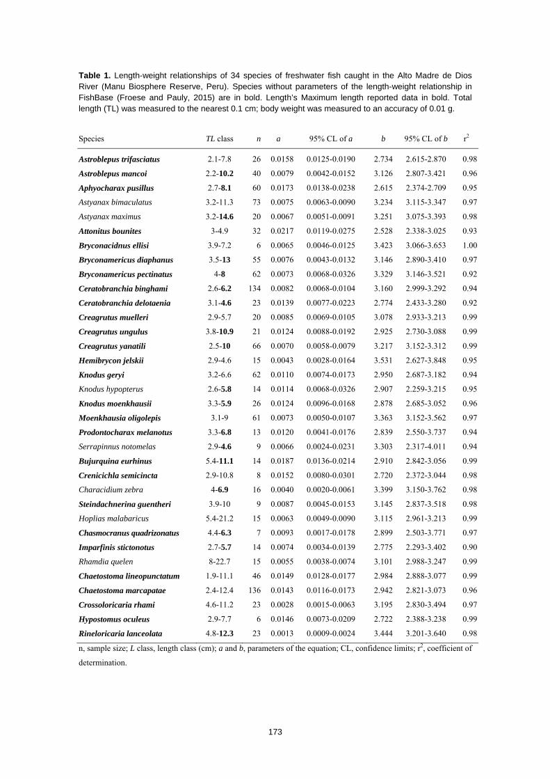
173
Table 1. Length-weight relationships of 34 species of freshwater fish caught in the Alto Madre de Dios River (Manu Biosphere Reserve, Peru). Species without parameters of the length-weight relationship in FishBase (Froese and Pauly, 2015) are in bold. Length’s Maximum length reported data in bold. Total length (TL) was measured to the nearest 0.1 cm; body weight was measured to an accuracy of 0.01 g.
Species TL class n a 95% CL of a b 95% CL of b r2
Astroblepus trifasciatus 2.1-7.8 26 0.0158 0.0125-0.0190 2.734 2.615-2.870 0.98
Astroblepus mancoi 2.2-10.2 40 0.0079 0.0042-0.0152 3.126 2.807-3.421 0.96
Aphyocharax pusillus 2.7-8.1 60 0.0173 0.0138-0.0238 2.615 2.374-2.709 0.95
Astyanax bimaculatus 3.2-11.3 73 0.0075 0.0063-0.0090 3.234 3.115-3.347 0.97
Astyanax maximus 3.2-14.6 20 0.0067 0.0051-0.0091 3.251 3.075-3.393 0.98
Attonitus bounites 3-4.9 32 0.0217 0.0119-0.0275 2.528 2.338-3.025 0.93
Bryconacidnus ellisi 3.9-7.2 6 0.0065 0.0046-0.0125 3.423 3.066-3.653 1.00
Bryconamericus diaphanus 3.5-13 55 0.0076 0.0043-0.0132 3.146 2.890-3.410 0.97
Bryconamericus pectinatus 4-8 62 0.0073 0.0068-0.0326 3.329 3.146-3.521 0.92
Ceratobranchia binghami 2.6-6.2 134 0.0082 0.0068-0.0104 3.160 2.999-3.292 0.94
Ceratobranchia delotaenia 3.1-4.6 23 0.0139 0.0077-0.0223 2.774 2.433-3.280 0.92
Creagrutus muelleri 2.9-5.7 20 0.0085 0.0069-0.0105 3.078 2.933-3.213 0.99
Creagrutus ungulus 3.8-10.9 21 0.0124 0.0088-0.0192 2.925 2.730-3.088 0.99
Creagrutus yanatili 2.5-10 66 0.0070 0.0058-0.0079 3.217 3.152-3.312 0.99
Hemibrycon jelskii 2.9-4.6 15 0.0043 0.0028-0.0164 3.531 2.627-3.848 0.95
Knodus geryi 3.2-6.6 62 0.0110 0.0074-0.0173 2.950 2.687-3.182 0.94
Knodus hypopterus 2.6-5.8 14 0.0114 0.0068-0.0326 2.907 2.259-3.215 0.95
Knodus moenkhausii 3.3-5.9 26 0.0124 0.0096-0.0168 2.878 2.685-3.052 0.96
Moenkhausia oligolepis 3.1-9 61 0.0073 0.0050-0.0107 3.363 3.152-3.562 0.97
Prodontocharax melanotus 3.3-6.8 13 0.0120 0.0041-0.0176 2.839 2.550-3.737 0.94
Serrapinnus notomelas 2.9-4.6 9 0.0066 0.0024-0.0231 3.303 2.317-4.011 0.94
Bujurquina eurhinus 5.4-11.1 14 0.0187 0.0136-0.0214 2.910 2.842-3.056 0.99
Crenicichla semicincta 2.9-10.8 8 0.0152 0.0080-0.0301 2.720 2.372-3.044 0.98
Characidium zebra 4-6.9 16 0.0040 0.0020-0.0061 3.399 3.150-3.762 0.98
Steindachnerina guentheri 3.9-10 9 0.0087 0.0045-0.0153 3.145 2.837-3.518 0.98
Hoplias malabaricus 5.4-21.2 15 0.0063 0.0049-0.0090 3.115 2.961-3.213 0.99
Chasmocranus quadrizonatus 4.4-6.3 7 0.0093 0.0017-0.0178 2.899 2.503-3.771 0.97
Imparfinis stictonotus 2.7-5.7 14 0.0074 0.0034-0.0139 2.775 2.293-3.402 0.90
Rhamdia quelen 8-22.7 15 0.0055 0.0038-0.0074 3.101 2.988-3.247 0.99
Chaetostoma lineopunctatum 1.9-11.1 46 0.0149 0.0128-0.0177 2.984 2.888-3.077 0.99
Chaetostoma marcapatae 2.4-12.4 136 0.0143 0.0116-0.0173 2.942 2.821-3.073 0.96
Crossoloricaria rhami 4.6-11.2 23 0.0028 0.0015-0.0063 3.195 2.830-3.494 0.97
Hypostomus oculeus 2.9-7.7 6 0.0146 0.0073-0.0209 2.722 2.388-3.238 0.99
Rineloricaria lanceolata 4.8-12.3 23 0.0013 0.0009-0.0024 3.444 3.201-3.640 0.98
n, sample size; L class, length class (cm); a and b, parameters of the equation; CL, confidence limits; r2, coefficient of
determination.
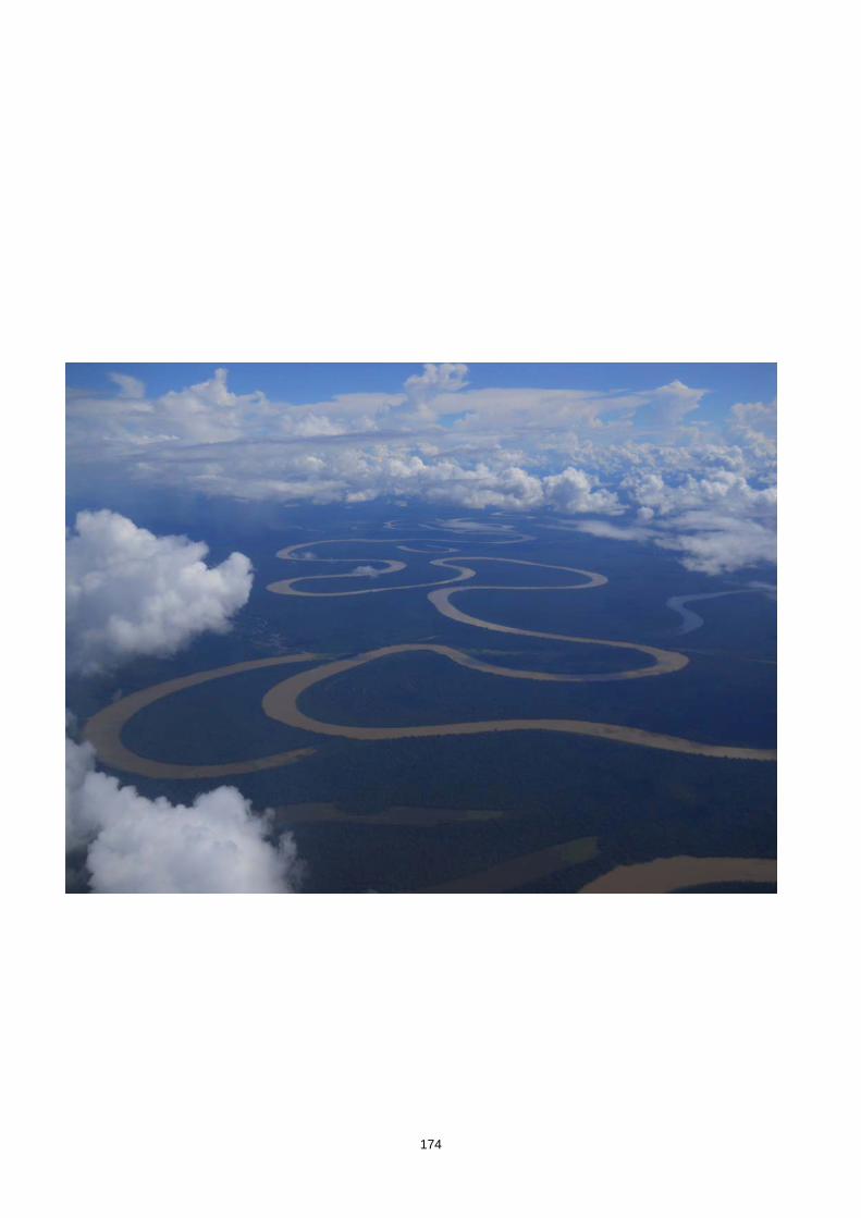
174

175
DISCUSIÓN GENERAL
GENERAL DISCUSSION

176
177
Evaluación de la metodología de muestreo
¿Es efectiva la pesca eléctrica?
La pesca eléctrica es la técnica más usada en la actualidad para llevar a cabo
estudios de la fauna piscícola en ecosistemas fluviales (Bain, Finn & Booke, 1985;
Paller, 1996; Pusey et al., 1998; Bertrand, Gido, & Guy, 2006; Survey, 2003), pero, tal
y como se mencinaba con anterioridad, existen discrepancias en cuanto a su eficacia en
ríos del neotrópico.
Para el desarrollo de esta tesis doctoral se llevaron a cabo un total de 75
muestreos de pesca eléctrica, 14 de ellos en el Pirineo español y 61 en el neotrópico. Las
pescas llevadas a cabo en España fueron en ríos que presentaban las condiciones
óptimas para las que fue desarrollada la técnica, y por ello los resultados fueron muy
buenos (Capítulo 1). Las poblaciones y abundancias de peces se correspondieron con lo
esperable para ríos de estas características, probando la robustez del método. Pero, en
cuanto a las 61 pescas eléctricas llevadas a cabo en el neotrópico, en Colombia
(Capítulo 2 y 4) y Perú (Capítulo 6), es posible que la eficacia del método fuera menor.
Esta incertidumbre sobre la efectividad de las colectas se debe a la falta de estudios que
nos sirvan de referencia para comparar y evaluar su eficacia. Aunque no pudiéramos
cuantificarlo, la impresión general era que en algunas localidades la técnica no resultaba
tan efectiva como al pescar en los ríos la Península Ibérica. Observábamos como había
peces que escapaban del rango de acción del equipo, por lo que posiblemente las
abundancias fueron subestimandas para algunos puntos de muestreo.
Solo para el caso de la cuenca del Alto Madre de Dios, en Perú, existía
información previa a nuestro trabajo. Un inventario llevado a cabo usando redes de
arrastre reportó un total de 130 especies de peces para toda la cuenca del río Madre de
Dios (Ortega, Corahua & Palacios, 2006). Nuestros muestreos de pesca eléctrica
sumaron un total de 78 especies, casi la mitad, aunque Ortega, Corahua y Palacios
abarcaron una extensión de cuenca mucho mayor, incluyendo zonas bajas, mientras que
nuestro esfuerzo se concentró en el territorio del río Alto Madre de Dios, la subcuenca
que conforma la cabecera.
178
También pudimos comparar nuestros resultados con un trabajo llevado a cabo
por Araujo-Flores (2015), quien inventarió con redes de arrastre una porción de la
cuenca del Alto Madre de Dios incluida en nuestros muestreos. De las 44 especies
reportadas por Araujo-Flores, solo 17 coincidieron con las 78 capturadas por nosotros.
Y al comparar las tres localizaciones de nuestro trabajo coincidentes con las
localizaciones de Araujo-Flores, frente a sus 44 especies nosotros capturamos solo 26,
aunque 15 de ellas estaban ausentes en el trabajo de Araujo-Flores.
A la luz de estos resultados, parece obvio que la eficacia de la pesca eléctrica es
significativamente menor en el neotrópico comparada con los ríos de zonas templadas,
especialmente al trabajar en grandes masas de agua y con conductividades muy bajas
(Penczak & Lasso, 1991). Estas limitaciones restringen la fiabilidad de la técnica a
pequeños ríos con suficiente conductividad (Pusey et al., 1998). Sin embargo, aunque la
técnica esté subestimando la abundancia de las especies, algunos autores destacan su
utilidad para llevar a cabo inventarios faunísticos, ya que la estimación de la riqueza de
especies parece no verse afectada (Allard et al., 2014). Además, parece ser que usando
la pesca eléctrica se capturan especies que escapan a los muestreos con redes, y con ella
pueden muestrearse con mucha efectividad pequeños ríos poco profundos en los cuales
las redes no resultan efectivas (Dewey, 1992).
Debido a las limitaciones demostradas por la pesca eléctrica y las redes, hay
autores que defienden el uso de rotenona en latitudes tropicales como la técnica más
fiable para completar estudios precisos de las comunidades de peces y sus abundancias
(Głowacki & Penczak, 2005). Aunque su efectividad sea incuestionable, intoxicar un río
y sacrificar toda la población de peces (y otros organismos con agallas) para poder
estudiarla no parece ser muy compatible con los objetivos de conservación. Sin
embargo, para ríos profundos o con conductividades muy bajas, la rotenona sigue
siendo el único método que permite estudiar de forma rápida y completa la comunidad
de peces (Allard et al., 2014).
Por todo ello, la pesca eléctrica parece ser una técnica fiable para llevar a cabo
inventarios de biodiversidad o para realizar estudios de comunidades y abundancias de
peces en ríos pequeños y con conductividades no demasiado bajas (Allard et al., 2014).
Aún así, parece recomendable complementarla con otras técnicas como las redes, sobre
todo en aquellos lugares donde pierde efectividad. Sin embargo, al ser una técnica
179
todavía poco habitual en latitudes tropicales donde la mayoría del esfuerzo científico se
ha centrado en grandes ríos y en especies de interés comercial, todavía existe un gran
vacío de conocimiento relativo a los ríos y especies me menor tamaño, para las cuales,
el uso de esta metodología puede resultar de gran utilidad (Mendonça, Magnusson, &
Zuanon, 2005).
¿Sirven las comunidades de peces y macroinvetebrados como bioindicadores?
Las comunidades biológicas, como parte del paisaje fluvial, están directamente
influenciadas por la intensidad y magnitud de las alteraciones antrópicas por lo que son
buenos indicadores de la integridad de los ecosistemas fluviales y sus cuencas (Allan,
2004). Sin embargo, carecer de una base ecológica sólida en la que basarnos puede
llevarnos a malinterpretar cambios naturales en la composición de las comunidades y
atribuirlos erróneamente a alteraciones antrópicas (Capítulo 3).
Afortunadamente, tanto para la península ibérica (Alba Tercedor et al., 2002)
(Capítulo 1) como para Colombia (Roldán, 2003) (Capitulo 2 y 4) ya existían
adaptaciones del índice BMWP que nos permitieron llevar a cabo diagnósticos de
calidad ambiental usando las comunidades de macroinvertebrados, con la seguridad de
que los resultados obtenidos eran fiables y representativos de las condiciones de los ríos
analizados.
Sin embargo, aunque también muestreamos los invertebrados acuáticos en la
cuenca del Alto Madre de Dios, en Perú (Capítulo 6), todavía no existe una adaptación
del índice BMWP para esta región, por lo que los resultados obtenidos, aunque
aparentemente consistentes, carecen de una base científica sólida que nos garantice la
fiabilidad del diagnóstico. Afortunadamente, recientes investigaciones están llevando a
cabo trabajos ecológicos que finalmente permitirán desarrollar un índice adaptado a
estos territorios (Medina et al., 2010).
El uso de esta técnica demostró su valía como herramienta diagnóstica y nos
permitió identificar aquellos lugares donde el río estaba más alterado (Capitulo 1, 2 y
4). Los resultados obtenidos fueron consistentes con las alteraciones detectadas en las
comunidades de peces, con los puntajes de los índices de calidad ambiental y con las
medidas de presencia de contaminantes, lo que refuerza y demuestra la fiabilidad de la
técnica.
180
Son también abundantes los estudios han probado el potencial de las
comunidades de peces como bioindicadores (Hued & Bistoni, 2005; Joy & Death, 2002;
Karr, 1981; Matthews & Hough, 1992), aunque todavía no existe para muchas regiones
un modelo estandarizado de respuesta ante el cambio, especialmente para regiones
neotropicales. Este conocimiento permitiría llevar a cabo diagnósticos precisos de la
integridad ecológica del río, identificando la presencia, origen e intensidad de los
impactos (Alexandre & Esteves, 2010).
Aun y todo, los resultados obtenidos mediante el presente trabajo de
investigación, aunque no nos permitan evaluar de forma cuantitativa el grado de
alteración del ecosistema basándonos en un puntaje relacionado con la presencia o
ausencia de taxones, o relativo a sus abundacias (tal y como se hace con los
macroinvetebrados), sí que nos han servido identificar posibles alteraciones en las
condiciones ambientales. Resulta especialmente notable el caso de Ordesa (Capitulo 1),
para el cual sí disponíamos de unas condiciones de referencia naturales sobre las que
trabajar, el río Ara. Sus características pusieron en evidencia la notable alteración de los
hábitats fluviales del río Gállego, en el cual habitaban especies de peces que en unas
condiciones originales nunca podrían haber sobrevivido. Sin embargo, hacer una
interpretación como esta para los ríos estudiados en el neotrópico es imposible, ya que
carecemos de información sobre las condiciones de referencia en las que basarnos.
Además, la correspondencia entre las comunidades de peces, sus abundancias y
su distribución han mostrado un patrón que encaja perfectamente con el diagnóstico
ambiental llevado a cabo usando los índices de calidad y las comunidades de
macroinvertebrados, lo que confirma su utilidad como bioindicadores (Muotka et al.,
1999, Carlisle et al., 2009). Sin embargo, los macroinvertebrados han demostrado ser
indicadores más sensibles a la contaminación de las aguas y degradación de hábitat a
escala local (Capítulo 2), posiblemente debido a su limitada movilidad y mayor
exposición a los impactos sobre el medio (Lammert & Allan 1999). Además, su
muestreo no presenta tantas limitaciones metodológicas como la pesca eléctrica y la
logística necesaria es más sencilla, lo cuál destaca su mayor versatilidad como
bioindicadores. Aun así, hemos observado que las comunidades de peces también
cambiaban ante impactos humanos, pero especialmente en respuesta a alteraciones a
escala de cuenca hidrográfica (Capitulo 2). Esto pone de manifiesto la necesidad de usar
tanto peces como macroinvetebrados como bioindicadores si queremos obtener

181
diagnósticos ambientales integrales, tanto a escala de tramo como a escala de cuenca
(Freund & Petty, 2007).
¿Sirven de los índices de calidad ambiental como herramientas de diagnostico?
Los índices de calidad ambiental han mostrado ser una herramienta fiable para
diagnosticar el estado de salud de los ríos. Los valores obtenidos por el QHEI (Rankin,
1989), IHF (Pardo et al., 2002) y QBR (Fornells, Solá & Munné, 1998) y sus
adaptaciones andinas (Acosta et al., 2008), han sido coherentes y han identificado
conjuntamente aquellos tramos más alterados (Capítulos 1, 2, 4 y 6). Además, su
diagnóstico ha sido consistente con el de las adaptaciones del BMWP (Alba Tercedor et
al., 2002; Roldán, 2003) y con la presencia de contaminantes. Es por ello que el uso de
estos índices puede considerarse como una herramienta fiable y fácil de usar para
evaluar la calidad ambiental.
Sin embargo, para poder contar con mayor objetividad a la hora de ser aplicados,
es recomendable que el muestreador sea el mismo, para que los criterios de valoración
se mantengan. Aunque los índices busquen ser lo más objetivos posibles y que cualquier
persona que los aplique llegue al mismo resultado, es imposible evitar cierta
subjetividad.
Aunque a menudo criticados, los índices de calidad ambiental han demostrado
ser una útil herramienta que nos ha ayudado a cuantificar y estandarizar observaciones
personales. Nos permiten evaluar y comparar el estado ecológico de forma empírica, y
nos obligan a analizar el ecosistema con más detalle y atención, ayudándonos a
comprender mejor aquello que estudiamos. Además, sus hojas de datos,
complementadas con fotografías y con el resto de los datos ambientales, pueden volver
a acercarnos a las orillas del río sin salir de la oficina de forma más objetiva que con un
simple recuerdo, pudiendo ser un gran apoyo a la hora de analizar e interpretar los
resultados.
Consideraciones generales y limitaciones de la metodología empleada
A la vista de los resultados, podemos afirmar que la metodología elegida ha
dado unos resultados suficientemente buenos para sentar una base de conocimiento allí
182
donde nada se sabía. Y su logística ha resultado lo suficientemente versátil como para
poder llevárnosla allí donde nadie había llegado antes a hacer ciencia.
Pero sin duda, uno de los mayores obstáculos, incluso mayor que la
inaccesibilidad y peligrosidad de los lugares elegidos, ha sido el tiempo. Siempre es el
tiempo. El tiempo limitado para poder llevar a cabo una campaña de muestreos siempre
ambiciosa. Ha sido él quien ha restringido el número de puntos de muestreo, pero, sobre
todo, su falta no nos ha permitido ir más que una vez a cada lugar. Por ello, los
resultados obtenidos deben ser interpretados desde esta limitación, ya que lo obtenido
ha sido una “foto” de un momento concreto para una realidad compleja y dinámica.
Los ríos son ecosistemas en constante cambio, “ningún hombre puede bañarse
dos veces en el mismo río”, así que, si queremos realmente saber que está pasando en
cada una de las cuencas estudiadas deberíamos seguir monitoreando. Para saber como
cambian el río y sus habitantes en las distintas estaciones, para valorar como responden
a impactos ambientales que no solo no cesan, sino que se intensifican, y para evaluar si
las medidas de protección están funcionando, resulta necesario prolongar la
investigación en el tiempo. Es por ello que nuestra fotografía ha dejado fuera del
encuadre gran parte de una compleja realidad ambiental.
Pero también nos han fallado las lentes. Solo hemos llevado una, la de la
biología. Y estas complejas realidades tienen una dimensión humana que no hemos
considerado más allá de las negativas consecuencias de su presencia. Hablamos de
gestionar ecosistemas, de desarrollo sostenible, aportamos información ecológica,
detectamos amenazas, pero no incluimos en nuestras investigaciones a las personas que
allí viven. ¿Cuál es su relación con los ríos, con el territorio, con los peces? ¿Cómo
podemos ayudarles de la mejor forma para que alcancen un desarrollo que les garantice
la armonía con el medio del que dependen? Son preguntas que dejamos sin responder.
Respuestas necesarias para conseguir un desarrollo consciente y cuidadoso con el
medio.
Utilidad de los trabajos descriptivos y relaciones de longitud-peso
Una de las ideas recurrentes en esta tesis doctoral es la falta de conocimiento
existente referente a los peces del neotrópico, y en concreto a las especies de los Andes
183
Tropicales (Albert & Reis, 2011). Este vacío, nos ha supuesto y supone para todos los
ictiólogos y ecólogos fluviales una barrera difícil de superar (Brooks et al., 2002).
Las consecuencias del impedimento taxonómico, en la práctica, se presentan así:
‐ Y este pez… ¿Qué será? ‐ Sí se parece a estos otros, ¿no? Entonces, manchita negra opérculo, aleta
amarilla. ¡Otro más! ‐ Y este… ¡Este no es lo mismo! Este es otra cosa… Es como estos otros, ¿no? ‐ Pues… ¿Sin manchita aleta amarilla? ¿Apunto otros siete? ‐ ¡Dale! Y este otro…
Aunque contamos con el apoyo de los principales expertos en ictiología de
Colombia (Javier Maldonado-Ocampo y José Iván Mojica) y Perú (Hernán Ortega), de
las 177 especies de peces colectadas en los Andes Tropicales 87 no pudieron ser
identificadas, quedando la mayoría clasificadas a nivel de género, con algunas pocas
que no pasaron del nivel de familia.
Este “impedimento taxonómico” (Taylor, 1983) y ecológico representa un
importante obstáculo para la biología de la conservación, y es por esto que resulta
prioritario llevar a cabo trabajos descriptivos e inventarios que permitan rellenar estos
vacíos de conocimiento (Abell et al., 2008). Estos trabajos descriptivos aportan una base
sistemática y taxonómica referencial, fundamentada en inventarios históricos y en la
constante actualización de catálogos y colecciones de biodiversidad (Nielsen & West,
1994). Desgraciadamente, aunque posean un valor intrínseco indiscutible, los trabajos
puramente descriptivos son cada vez más escasos debido a las dificultades existentes a
la hora de publicarlos en revistas científicas (sustento y vara de medida para un
investigador), y son habitualmente infravalorados y rechazados (Underwood, 1996). Es
por ello que los estudios ecológicos descriptivos tan comunes en el pasado, los grandes
inventarios taxonómicos de la era de los exploradores, son minoritarios en el siglo XXI.
Este “impedimento taxonómico”, un problema endémico del neotrópico, ha dado
lugar a un movimiento “parataxonómico” llamado “suficiencia taxonómica”, un
enfoque pragmático para esquivar el problema (Ellis, 1985). Esta idea se acabó
convirtiendo en algo común para la biología de la conservación y dio lugar a que la
riqueza de taxones o unidades taxonómicas sustituyeran a la riqueza de especies (Faith,
1994). Sin embargo, solo el uso del más preciso nivel de clasificación, la especie,
184
garantiza unas estimaciones de biodiversidad consistentes y comparables (Pleijel &
Rouse, 2000).
En nuestro caso, para salvar este obstáculo hemos abordado el estudio de la
ecología de los peces a nivel de género. Pero sin duda es insuficiente. Al trabajar a esta
escala asumimos que todos los peces del mismo género compartirán ciertas preferencias
de nicho, y así, estudiamos su ecología de forma conjunta. Pero las evidencias nos
muestran que en muchos casos puede resultar insuficiente tal y como se expondrá más
adelante.
Por ello, además de la utilidad innegable de los trabajos descriptivos, resultan
igualmente valiosos los reportes de relaciones de longitud-peso de las diferentes
especies colectadas (Capítulos 3, 5 y 7). Aunque aparentemente tengan una relevancia
menor, aportan una información que puede ser muy útil en varios contextos: pueden ser
usadas a la hora de desarrollar planes de pesca selectiva y sostenible, ya que nos
proporcionan una información con la que adaptar la luz de las redes para capturar
ciertos individuos y dejar escapar a otros (Almeida, Lorenzen & McGrath, 2003); sirven
de referencia para comparar poblaciones de diferentes lugares pudiendo poner en
evidencia inconsistencias taxonómicas (Doadrio, Carmona & Fernandez-Delgado,
2002); nos informan del estado de los peces y sus poblaciones, ya que gracias a ellas
podemos ver si hay peces de todas las edades (Appelberg et al., 1995), si la población es
estable y tiene un buen reclutamiento (Gabelhouse, 1984), si los peces están en buenas
condiciones físicas, o si por el contrario existen problemas que estén afectando a las
comunidades (Froese, 2006). Así, el estudio de las tallas de los peces puede resultar
también una herramienta muy útil a la hora de detectar alteraciones ambientales, e
incluso puede ser usada sin falta de conocimiento taxonómico, permitiéndonos evaluar
el estado de las comunidades de peces y la integridad del ecosistema allí donde la
información existente sea escasa (Benejam et al., 2015).
Biodiversidad y ecología de las cuencas estudiadas
La influencia de las condiciones ambientales en los ríos: la altitud como variable
Una de las principales líneas de investigación en ecología, y uno de los objetivos
principales de esta tesis doctoral, ha sido determinar cómo las características
185
ambientales, a escala de paisaje y escala local, conforman distintos hábitats y limitan la
distribución de las especies.
El estudio de los gradientes ambientales y la influencia que tienen sobre los
patrones de distribución de los organismos en ecosistemas fluviales tiene una larga
historia. En el caso de la composición y distribución de las comunidades de peces, estos
patrones han sido asociados con cambios temporales y espaciales en la morfología de
los cauces y la disponibilidad de recursos (Schlosser, 1982), a los cambios en el caudal
(Taylor et al., 1996), al tamaño del río y su cubierta vegetal (Angermeier & Karr, 1983),
al tamaño del río y la velocidad del agua (Meffe & Sheldon, 1988), al tamaño del río y
la alcalinidad de sus aguas (Peterson & Gale, 1991), a la presencia de barreras (caídas
de agua) y cambios en la estructura de los hábitats (Pusey et al., 1998), al régimen
termal de las aguas, la ecoregión y el tamaño del río (Lyons, 1996), o a cambios
graduales en el hábitat (sustratos, profundidad, cantidad y tipo de refugio disponible)
(Angermeier & Karr, 1984).
También son abundantes los trabajos que han estudiado la influencia de las
variables ambientales en la distribución longitudinal de los peces en el neotrópico.
Ibarra & Steward (1989) atribuyeron los cambios en las comunidades a lo largo del
gradiente longitudinal de los ríos a los grandes cambios en la composición del sustrato
(dominancia de rocas y cantos rodados en zonas altas y su ausencia en los tramos
bajos). Abes y Agostinho (2001) relacionaban la diversidad de especies con el orden del
río, y afirman que según este aumenta los mesohábitats también aumentan de tamaño y
se vuelven más diversos, dando lugar a una mayor diversidad de peces. Casatti & Castro
(1998) hablan de la velocidad del agua y el tipo de sustrato como los principales
factores que configuran las comunidades de peces y Reyes-Gavilán (1996) concluye
que, en términos generales, las varaciones en la composición de especies a lo largo del
curso del río están determinados por factores abióticos en los tramos de cabecera y por
las interacciones bióticas en las zonas bajas.
Existe también una marcada tendencia que analiza la variación de las
comunidades de los organismos acuáticos en relación al gradiente altitudinal y que
relaciona los rangos de distribución de las especies con la elevación (Schlosser, 1982;
Ormerod et al., 1994; Tejerina-Garro et al., 2005; Miranda-Chumacero, 2006; Nogués-
Bravo et al., 2008; Jaramillo-Villa, Maldonado-Ocampo, & Escobar, 2010; Lorion,
186
Kennedy, & Braatne, 2011; Lujan et al., 2013). Esto es también habitual para muchos
trabajos de investigación llevados a cabo en los ríos de los Andes. Bistoni & Hued
(2002) relacionaron para los ríos argentinos la riqueza de especies con la altitud, la
distancia al origen y el orden del río. Otros trabajos en Chile (Campos, 1982), Ecuador
(Ibarra & Steward, 1989), Colombia (Jiménez et al., 1998) y al sureste de Brasil (Abes
& Agostinho, 2001) relacionaron los patrones de distribución de especies y sus
comunidades con las condiciones físico-químicas del agua y la altitud.
Pero esto es un error, ya que la altitud no es una variable ambiental, es una
variable geográfica, de posición. Nos indica dónde está el punto de muestreo respecto al
nivel del mar. Por ello, incluir la altitud como un variable que condiciona las
características del río puede dar lugar a interpretaciones erróneas, ya que son las
características del territorio y no la altitud las que definen los límites entre zonas
hidrobiológicas. Aun así, la elevación está sin duda en estrecha relación con las
variables ambientales, y comparando tramos a lo largo del mismo río a diferentes
altitudes podemos afirmar casi con total seguridad que, cuanto más abajo, el agua estará
más caliente, menos oxigenada, tendrá mayor conductividad, fluirá más despacio, etc.
Pero esto no quiere decir que dos lugares situados a la misma altitud en dos ríos
diferentes vayan a compartir valores ambientales.
Si analizamos esta problemática en base a nuestros resultados, vemos que en el
río Hacha, por encima de los 300 metros, aún teníamos un ecosistema con marcado
carácter montañoso con unas comunidades adaptadas a sus hábitats particulares
(Capítulo 2). Sin embargo, en el Alto Madre de Dios, a los 700 metros, el río ya se
volvía de llanura y la composición de especies cambiaba notablemente (Capítulo 6). Y
en la cuenca del río Suaza (con un nivel base mucho más elevado al tratarse de un valle
interandino) este salto ecológico ocurría a los 1280 metros de altitud (Capítulo 4).
Es por ello que, la altitud es una variable relativa que no puede tomarse como
referencia para comparar diferentes cuencas, y que además no explica la variabilidad
ambiental sino la espacial. Así, incluirla como variable ambiental en los análisis
estadísticos es un error. También porque es una variable redundante, ya que los cambios
del resto de los factores medidos a lo largo de su curso (e.g. oxígeno, temperatura,
conductividad) nos aportan ya esta información sobre el cambio gradual a lo largo del
río.
187
Diversidad, riqueza y dominancia
Tal y como se exponía anteriormente, podemos atribuir el rango de distribución
de los peces a un aumento en la cantidad y heterogeneidad de los hábitats disponibles,
los cuales ofrecen una mayor variedad de recursos alimenticios y refugios aguas abajo
(Matthews, 1998, Walters et al., 2003). Este aumento en la diversidad de hábitats está
directamente relacionado a los cambios en la geomorfología, los cuales influencian
directamente la estructura de las comunidades de peces a lo largo de los gradientes
altitudinales (Robinson & Rand 2005) y crean un gradiente de productividad biológica
que aumenta aguas abajo. Es por ello que la diversidad de especies es mayor cuanto más
alejado está el tramo de su origen, y, por el contrario, la dominancia de unas pocas
especies se reduce con el aumento del número de especies (Schlosser, 1982). Este
aumento en la riqueza aguas abajo se incrementa a un ritmo mucho mayor en latitudes
tropicales en comparación con zonas templadas (Welcomme, 1979).
Este fenómeno se ha visto claramente reflejado en los ecosistemas estudiados.
En las tres cuencas de los Andes Tropicales, la riqueza y diversidad de especies
aumentaba significativamente aguas abajo, mientras que la dominancia de especies
disminuya de forma proporcional (Capítulos 2, 4 y 6).
No ha sido así sin embargo para el caso de Ordesa (Capítulo 1). Además de que
el aumento de la riqueza de especies es mucho menor en climas templados, los ríos
estudiados se restringían a zonas de cabecera donde de forma natural solo habita una
especie, Salmo trutta, tal y como se observó en el río Ara. Es por ello que el aumento en
la diversidad de especies del río Gállego es una consecuencia directa de las alteraciones
del hábitat debidas a presiones antrópicas. Es posible que este mismo fenómeno esté
ocurriendo en los ríos de los Andes, pero la falta de referencias de las condiciones
originales nos impide atribuir el aumento en la riqueza de especies a los impactos
humanos.
Sinecología fluvial: quién, dónde y por qué
Llegados hasta aquí resulta evidente que la composición y distribución de las
comunidades de peces responden directamente a las condiciones ambientales y a la
diversidad y abundancia de otros organismos. Estos procesos sinecológicos han sido ya
analizados en cada capítulo, caso por caso para, cada una de las cuencas. A
188
continuación, intentaré hacer una interpretación en conjunto de como las variables
ambientales determinan la distribución de los peces.
Tal y como se ha comentado anteriormente, existe una clara zonificación de las
cuencas fluviales marcada por las variables geomorfológicas e hidrobiológicas. Se
pueden identificar por ello dos regiones marcadamente diferentes, las cabeceras y las
zonas de llanura, y entre ambas, podemos identificar una zona de transición o curso
medio.
Sin embargo, resulta muy difícil establecer un criterio geográfico o espacial que
nos permita definir estas zonas de forma conjunta para todas las cuencas estudiadas, ya
que este cambio de zona de cabecera a curso medio se da por una acumulación gradual
de influencias ambientales. La lógica nos empuja a pensar en rangos altitudinales que
nos permitan establecer los límites, pero tal y como se ha expuesto anteriormente,
resulta una aproximación errónea. Por lo tanto, la zonificación que a continuación se
presenta responde a unos rasgos comunes agrupan tramos fluviales por sus
características ambientales. Pero, como incluso bajo esta visión resulta difícil establecer
un límite concreto. El criterio usado responderá también a cambios significativos en la
composición de la comunidad de peces, lo cual es un signo inequívoco de un cambio en
el hábitat.
Las composición de las comunidades y su distribución a lo largo de las cuencas
presentadas a continuación muestran patrones similares a los descritos por estudios
anteriores, lo cual refuerza nuestros resultados, tanto para las cuencas de los Andes
Tropicales (Angermeier & Karr, 1983; Arratia, 1983; Winemiller, 1983; Sabino &
Castro, 1990; Flecker, 1997; Aranha et al., 1998; Sabino & Zuanon, 1998; Mazzoni &
Lobón-Cerviá, 2000; Lemes and Garutti, 2002; Tejerina-Garro et al., 2005; Cotapata &
Miranda-Chumacero, 2006; Nogués-Bravo et al., 2008; Jaramillo-Villa, Maldonado-
Ocampo, & Escobar, 2010; Lorion, Kennedy, & Braatne, 2011; Lujan et al., 2013),
como para las cuencas pirenaicas (García de Jalon et al., 1988; García de Jalón,
González de Tánago, & Casado, 1992; García de Jalón, Mayo, & Molles, 1996; Alonso-
González et al., 2008; Leunda et al., 2009; Miranda et al., 2012).
189
Ríos de cabecera
Estas zonas definidas como cabeceras abarcan un rango altitudinal muy amplio
al comparar las diferentes cuencas. Considerando la elevación de nuestros puntos de
muestreo en los Andes Tropicales, para la cuenca del río Hacha iría desde los 2132 m
hasta los 1341, en el río Suaza se extiende desde los 1880 m hasta los 1445 m, y en el
Alto Madre de Dios desde los 2132 m hasta los 1341 m. En todos los casos el límite lo
ha marcado la aparición de las primeras especies detritívoras-herbívoras lo cual nos
indica que los ríos han dejado de ser excluyentemente oligotróficos (Chaetostoma en el
Hacha, Chaetostoma y Ancistrus en el Alto Madre de Dios y Saccodon dariensis en el
Suaza).
En el caso de los ríos Gállego y Ara podríamos hablar de que toda la cuenca
estudiada pertenece a zonas de cabecera. Aunque en las zonas más bajas de ambas
cuencas (en torno a los 850 m) las características geomorfológicas empiecen a cambiar,
si nos fijamos en la comunidad de peces, en el caso del Ara solo encontramos Salmo
trutta, lo que nos lleva a pensar que el río todavía conserva su carácter de río de
cabecera. Es verdad que en el Gállego encontramos especies exclusivamente herbívoras
ya a los 1077 m, pero esto se debe a una fuerte alteración humana de los hábitats, por lo
que tomaremos como referencia las características naturales del Ara y agruparemos
todos los sitios de estudio dentro de la categoría de ríos de cabecera.
Los ecosistemas fluviales situados en las partes más altas de las cuencas
comparten unas características comunes. Son ríos más pequeños: más estrechos, menos
profundos y menos caudalosos, pero expuestos también a bruscas crecidas y estiajes. El
dosel arbóreo cubre sus cauces sombreando los ríos y aportando materia orgánica. Sin
embargo, este aporte alóctono de nutrientes es todavía escaso, por lo que sus aguas son
bastante oligotróficas y apenas presentan vegetación acuática. Las fuertes pendientes
hacen que sus aguas fluyan más torrentosas, oxigenándose mucho. Además, al ser las
nacientes, la conductividad y la temperatura del agua son menores, y los sustratos son
de mayor tamaño que aguas abajo.
Estas características ambientales ejercen una fuerte presión selectiva sobre los
peces, siendo especialmente limitante la escasa disponibilidad de alimento. Por ello, son
unas pocas especies reófilas y exclusivamente invertívoras las que los habitan. Esta baja
190
diversidad y marcada dominancia de unas pocas especies es un mecanismo
compensatorio de las poblaciones que se adaptan a la escasa disponibilidad de recursos
(Matthews, 1998; Lomolino, 2001).
Aparecen buenos nadadores que habitan la columna de agua, como Salmo trutta,
única especie presente en las cabeceras de los ríos pirenaicos, mientras que en los Andes
Tropicales destaca la presencia de los Bryconamericus, que, aunque no está presente en
las localidades más altas (aparece a los 1400 m en el Alto Madre de Dios y a los 1615 m
en el Suaza) es uno de los primeros géneros en aparecer. Sin embargo, aunque este
género esté habitualmente relacionado con ríos de cabecera (Román-Valencia &
Muñoz, 2001), en la cuenca del río Hacha apareció solo en pequeños ríos de zonas más
bajas (~300 m).
Sin embargo, los peces más comunes en todas las cabeceras andinas son los
Astroblepus. Son peces invertívoros bentónicos muy adaptados a las fuertes corrientes.
Cuentan con una ventosa en la boca con la se pegan a las rocas y unas aletas espinosas
que usan para arrastrarse contracorriente sin despegarse del sustrato. Aunque están
principalmente asociados a las cabeceras de los ríos, tal y como se ha visto en el caso
del río Hacha y el río Suaza, abarcan un amplio rango altitudinal (4600-100m)
apareciendo a los 424 en la cuenca del Alto Madre de Dios (Schaefer & Arroyave,
2010). Además, tienen un amplio rango territorial y pueden encontrarse desde Panamá
hasta Bolivia (Jaramillo-Villa et al. 2010; Anderson & Maldonado-Ocampo, 2011).
Acompañando a los Astroblepus suele ser habitual encontrar distintas especies
de Trichomycterus, tal y como ocurrió en la cabecera del Alto Madre de Dios (Capítulo
6). Son peces que también aparecen a lo largo de un amplio rango altitudinal, que
pueden aparecer estrechamente relacionados y adaptados a zonas altas de las cuencas,
pero que, así como los Astroblepus están presentes en la mayoría de las cabeceras
andinas, los Trichomycterus no siempre muestran este mismo patrón. Por ejemplo, no se
halló ninguno en la cuenca del río Hacha (Capítulo 2), y en el río Suaza aparecieron por
primera vez a los 1240 m, en la zona media de la cuenca (Capítulo 4).
Cabe destacar que, aunque la diversidad local de estas zonas de cabecera sea
muy baja en comparación con los cursos bajos de sus cuencas, si estudiamos su
diversidad a escala andina muchas de las comunidades y especies de estos ríos son
191
únicas, lo que pone de manifiesto su elevada diversidad β. Es por ello que estas zonas
de cabecera, aunque poco diversas en cuanto al número total de especies que albergan,
tienen un gran valor ya que estas especies tienen altas tasas de (Schaefer & Arroyave,
2010).
Curso medio
Después de haber clasificado las dos cuencas del Pirineo como zonas de
cabecera, la categorización como curso medio y curso bajo será exclusiva de los ríos de
los Andes Tropicales.
Tal y como se mencionaba con anterioridad, las cuencas estudiadas están
claramente divididas en dos zonas marcadamente diferentes, las cabeceras y las zonas
más bajas. Sin embargo, entre medio encontramos una zona de transición, tanto
ambiental como biológica, en la cual seguimos encontrando las especies que habitan
exclusivamente las cabeceras, como los Astroblepus, junto con especies con marcada
preferencia por ríos de curso bajo, como pueden ser los Ancistrus. Es por eso que resulta
más complejo establecer unos límites claros que sean iguales para las tres cuencas a
estudio. Aún y todo, si observamos los cambios en la composición de especies y
también tenemos en cuenta la aparición de un nuevo nicho trófico, las especies
piscívoras, podemos hacer una nueva categorización.
Estos ríos de transición ya portan mayores cantidades de agua y son más anchos
y profundos. Aunque los ríos de esta zona también estén sujetos a grandes crecidas, el
agua desbordará en las llanuras de inundación que ya se empiezan a formar al ir
abriéndose los valles, por lo que su carácter erosivo empieza a cambiar a sedimentario.
Además, sus cauces con pendientes cada vez más moderadas muestran una
geomorfología muy bien definida y estable, alterando rápidos y pozas. Es por esto que
la diversidad de sustratos aumenta significativamente, y además de encontrarnos todavía
grandes rocas y cantos rodados típicos de las zonas de cabecera, aparecen también
gravas, arenas, limos y arcillas. Por todo ello, la diversidad de hábitats aumenta, así
como la diversidad y cantidad de recursos tróficos, por lo que la diversidad ictiológica
crece también.
En el caso del Alto Madre de Dios, resulta complicado establecer el límite entre
esta zona y la zona de llanura, ya que el solapamiento de especies es bastante notable
192
entre ambas. Sin embargo, es significativo el salto en riqueza de especies que ocurre en
torno a los 700 m, y destaca también la aparición de las primeras especies piscívoras a
los 620 m, por lo que parece que el límite inferior del curso medio podría situarse en
este rango altitudinal. En cuanto a las especies más características de esta comunidad
destacan las de los géneros Characidium, Rhamdia, Creagrutus y Chasmocranus.
Para el río Suaza también es difícil definir un límite entre la cuenca media y
cuenca baja, aunque ateniendo de nuevo a la composición de especies y a las
características ambientales, es posible apreciar una diferenciación entre los tres sitios
más bajos, situados a partir de los 1101 m, y los otros tres de curso medio, entre los
1280 y 1205 m. Las especies características de esta zona media pertenecen en este caso
a los géneros Trichomycterus y Characidium. Ambos géneros aparecen también en el
curso medio del Alto Madre de Dios. Sin embargo, mientras que los Trichomycterus
aparecen en el Alto Madre de Dios estrechamente relacionados con las zonas de
cabecera, resulta llamativo que en el Suaza no aparezcan en las zonas altas y estén
relacionados con el curso medio del río.
Esta distribución poco predecible del género Trichomycterus (también observada
previamente para el género Bryconamericus) pone en evidencia las carencias resultantes
de llevar a cabo análisis ecológicos a nivel de género, tal y como se mencionaba con
anterioridad.
Por último, en el caso del río Hacha encontramos un curso medio más extenso
que en los otros casos, el cual abarca un rango altitudinal desde los 1341 hasta los 282
m. Esto se debe a que las pendientes de los Andes se extienden hasta ese punto, lugar en
el que abruptamente dan paso a la llanura amazónica. Tal y como ocurría en el río Suaza
y Alto Madre de Dios, volvemos a encontrar peces del género Characidium como
característicos del curso medio, a los que se suman los Chasmocranus y Creagrutus,
también presentes en el curso medio del Alto Madre de Dios. Además, completan la
comunidad especies pertenecientes a los géneros Cordylancistrus, Boehlkea, Astyanax y
Parodon.
Curso bajo
En las zonas más bajas de las cuencas, donde los ríos ya abandonan
definitivamente las laderas de las montañas y se abren a las grandes llanuras, la
193
pendiente se reduce considerablemente, los ríos se anchan, la velocidad de la corriente
baja y se forman hábitats con aguas calmadas, pozas y remansos. La dinámica del río
cambia de erosiva a sedimentaria. Los cauces se cubren de materiales finos. Las aguas
son más calientes, con mayor conductividad y abundantes en nutrientes, tanto por todos
los arrastrados desde el curso alto como por los autóctonos, lo que aumenta
significativamente la producción primaria (Winemiller et al., 2008). Además, la gran
cantidad de materia orgánica que se deposita en el lecho del río da lugar a que la
mayoría de las especies de peces que habitan estas zonas sean de hábitos bentónicos. Se
trata del comienzo de las extensas y diversas cuencas bajas de los grandes ríos del
subcontinente americano.
Acompañando el marcado salto geomorfológico, las comunidades de peces
cambian notablemente y la cantidad de especies crece significativamente. Aparecen ya
especies exclusivamente piscívoras como los Hoplias malabaricus (presente en el río
Hacha y en el Alto Madre de Dios) o los Crenicichla semicincta (en el Alto Madre de
Dios) debido a un aumento en las poblaciones de peces que se convierten en recurso
trófico.
Las comunidades que definen el tramo bajo en el río Suaza las componen peces
de los géneros Lasiancistrus, Pimelodella, Chaetostoma, Rhamdia y Parodon, que
abarcarían para nuestro caso de estudio un rango altitudinal desde los 1101 a los 997 m.
En el caso del Alto Madre de Dios, a partir de los 700-600 m, encontramos dos
comunidades de peces relacionadas con las zonas bajas de la cuenca, pero diferenciadas
por sus preferencias de hábitat. Por un lado, tenemos a los géneros Astyanax, Knodus,
Creagrutus y Corydoras, asociados a pequeños afluentes con sustratos finos, aguas con
conductividades algo más altas y con presencia de abundante materia orgánica en
descomposición. Y por otro lado están los tramos en los cauces principales, más anchos,
con presencia de guijarros y con aguas más rápidas, donde encontramos peces de los
géneros Hemibrycon, Rineloricaria, Chaetostoma y Ancistrus.
Por último, en la cuenca del río Hacha, a partir de los 282 m ocurre un drástico
cambio en las características de los ríos y de sus comunidades de peces, mucho más
marcado que en las otras cuencas estudiadas. Tanto la diversidad como la abundancia
aumentan de forma muy significativa y repentina, y la comunidad de peces es mucho
194
más compleja que en los otros casos, conformada por peces de los géneros Farlowella,
Bunochephalus, Leporinus, Imparfinis, Loricaria, Loricariichthys, Odontostilbe y
Pimelodella, así como varias especies de las familias Characidae y Cichlidae.
Este brusco cambio está intensificado por la presencia de la ciudad de Florencia,
situada en las últimas estribaciones de la cordillera y en el comienzo de la llanura
amazónica. Concretamente, el punto de corte entre las comunidades de curso medio y
bajo lo marca la desembocadura en el río Hacha de un afluente que recibe la mayoría de
las aguas residuales de la ciudad.
Al solaparse el cambio en la geomorfológia del paisaje con las alteraciónes
producidas por la ciudad de Florencia, resulta imposible determinar en qué medida la
comunidad de peces del curso bajo del río Hacha es natural o está alterada por los
impactos humanos. Esto se debe a que no contamos con información previa al impacto
ni con unas condiciones de referencia con las que comparar.
Desgraciadamente este escenario es habitual. En la cuenca baja los ríos
abandonan los valles cerrados y empinados de las laderas de las montañas y se abren en
anchos valles con fértiles llanuras, paisajes mucho más adecuados para los
asentamientos humanos y el aprovechamiento de los recursos naturales. Es por esto que
los cursos bajos de los ríos están mucho más expuestos a alteraciones, y muchos ya
sufren marcados procesos de degradación de hábitats.
Uno de los cambios más notables es una producción y diversidad de peces
mayor a la esperada. Las zonas urbanas aportan con sus vertidos grandes cantidades de
materia orgánica lo que aumenta artificialmente la productividad total del río (Mazzoni
& Lobón-Cerviá, 2000). Para entender la influencia que estas aguas residuales pueden
tener basta con comparar la comunidad de peces de los puntos H08 y H09 en la cuenca
baja del río Hacha. Tal y como se exponía anteriormente, ambos puntos están situados
muy cercanos dentro del río Hacha y presentan características de hábitat similares, pero
los separa la desembocadura de un afluente que recibe la mayoría de las aguas urbanas.
Es tal la alteración que ocasionan las aguas residuales que las comunidades de peces de
ambos puntos son totalmente diferentes. La comunidad del tramo anterior al vertido se
agrupa con la de los ríos de curso medio, mientras que el otro tramo, apenas situado 500
195
metros aguas abajo, presenta una comunidad de peces totalmente diferente,
característica de los tramos más bajos de la cuenca.
Esta influencia de los impactos humanos ha sido también notable en el caso de la
Reserva de la Biosfera de Ordesa-Viñamala (Capítulo 1). El río Ara apenas tiene
influencia antrópica y en sus aguas capturamos 303 peces en 6 puntos de muestreo,
todos ellos Salmo trutta. Sin embargo, en la cuenca del Gállego, donde la alteración de
los ecosistemas por impactos humanos es bastante mayor, las diferencias fueron
notables: 1674 peces en 8 puntos de muestreo, y tres especies nuevas muy alejadas de
su rango de distribución natural.
Queda en evidencia por lo tanto la drástica influencia que tienen las alteraciones
antrópicas sobre los ríos y sus organismos. Es por ello que si queremos conservar estos
ecosistemas y su biodiversidad necesitamos entender mejor los mecanismos naturales
que conforman sus procesos y que condicionan la distribución de la fauna a lo largo del
río. Además de que resulta esencial contar con unas condiciones de referencia, es muy
importante también que estudiemos las consecuencias de los impactos que causamos a
los ríos, que midamos su intensidad, que identifiquemos las tipologías de las
alteraciones y busquemos soluciones para paliarlas.
Identificar y definir zonas prioritarias para la conservación: los Andes Tropicales
Llegados hasta aquí, parece indiscutible la necesidad de actuar de forma
inmediata y efectiva para salvaguardar la biodiversidad del planeta. La identificación de
los hotspots mundiales para la conservación de la biodiversidad llevada a cabo por
Myers et al., (2000), facilita el trabajo a la biología de la conservación y permiten
focalizar los esfuerzos en territorios prioritarios. Este es el caso de los Andes
Tropicales, considerado el más diverso de todos los hotspot del planeta, cuya
denominación geográfica, aunque útil, presenta ciertos problemas.
Para el caso de los peces de agua dulce, los Andes Tropicales abarcan en su
territorio un total de 380 especies, de las cuales 131 son endémicas (Mittermeier et al.,
2011). Si comparamos estos datos con las 6000 (Reis et al. 2003) y las 8000 especies de
peces de agua dulce estimadas para todo el neotrópico (Vari & Malabarba, 1998),
parece ser que la diversidad de esta denominación biogeográfica está ampliamente
subestimada (Anderson & Maldonado-Ocampo, 2011). Esto puede deberse en parte a la
196
notable falta de información referente a este grupo de vertebrados, tal y como se ha
expuesto con anterioridad, y a que es habitual que estos sean excluidos de los estudios
de biodiversidad y los planes de conservación (e.g., Myers et al. 2000). Además, no
debemos olvidar que la naturaleza tiene un carácter continuo, gradual, por lo que al
establecer límites artificiales nos encontramos ante la imposibilidad de trazar fronteras
claras y concretas que se adapten a nuestras necesidades.
Esta problemática surge a escala local, tal y como se exponía anteriormente a la
hora de definir zonas a lo largo de una cuenca fluvial, pero también a escala continental.
Este es el caso de la delimitación del hotspot de los Andes Tropicales. Si analizamos su
definición geográfica, parece que su distribución latitudinal está bastante bien definida
por el paso de la cordillera por regiones y climas tropicales, lo cual marca unos límites
ecológicos claros. Sin embargo, al analizar su rango altitudinal, nos encontramos con
que el límite inferior está fijado a los 500 m, a la misma altura a lo largo de toda la
cordillera (Myers et al., 2000).
Esta frontera se basa en la existencia de un punto de inflexión notable a lo largo
del piedemonte andino, en el cual la riqueza de especies aumenta muy
significativamente y la composición de las comunidades cambia (Romero, Cabrera &
Ortiz, 2008). Tal y como se ha presentado anteriormente, este salto de hábitats
montañosos a ecosistemas de llanura también es notable para los ríos. No obstante, tal y
como se ha visto para el caso del río Hacha, los hábitats de curso alto y medio se pueden
llegar a extender hasta una elevación de 300 m. Además, estos tramos están habitados
por unas comunidades de peces diversas y estrechamente ligadas a esos territorios de
transición, todavía dependientes del influjo montañoso.
Es por ello que establecer el límite de lo que son o no son ecosistemas de los
Andes Tropicales basándonos en la altitud vuelve a traernos problemas. Esta frontera
artificial deja fuera de su denominación geográfica partes del piedemonte andino que
por sus características hidrogeomorfológicas se corresponderían con ecosistemas
fluviales de montaña (Lujan et al., 2013). Estudios más recientes estiman que pueden
ser más de 600 especies de peces las habiten los ríos de los Andes Tropicales, con una
tasa de endemismo del 40%: Colombia alberga 223 especies andinas, Ecuador 92, Perú
123 y Bolivia 155 (Anderson & Maldonado-Ocampo, 2011).
197
Por todo ello, una vez hecho el trabajo a gran escala, después de haber
identificado y definido grandes territorios cuya protección debe ser prioritaria, resulta
esencial considerar la casuística regional para adaptar los planes de gestión a cada
realidad concreta. Además, esta política debe ser aplicada tanto a la luz de las
cambiantes condiciones ambientales como de su dimensión y contexto social (Moulton
& Wantzen, 2006).
¿Protegen las áreas protegidas?
Las áreas protegidas son reconocidas ampliamente como esenciales para la
conservación de la biodiversidad mundial (Gaston et al., 2008; Chessman, 2013), pero
¿realmente consiguen sus objetivos, y sirven en este caso concreto para proteger los
ecosistemas fluviales y su biota?
Los ríos son ecosistemas unitarios, continuos e interdependientes, constituidos
por todo el territorio que drena a sus cauces (Lammert & Allan, 1999).
Consecuentemente, deberíamos tomar en cuenta todos los procesos ecológicos que los
conforman y configuran, y entender y considerar su estrecha conexión con toda la
superficie que integra su cuenca hidrográfica (Allan, 2004). Desgraciadamente, los ríos
son frecuentemente usados para trazar límites territoriales, también a la hora de
delimitar áreas de conservación (Nel et al., 2007). Esto tiene unas consecuencias
negativas importantes, tal y como se analizaba en el Capítulo 1 para la cuenca del río
Gállego. Aunque uno de los márgenes de la cuenca esté bajo la más estricta protección,
si en la otra orilla no existen restricciones al uso del territorio, el río está totalmente
expuesto a la trasmisión de impactos provenientes del territorio colindante.
Otro de los principales errores cometidos al establecer áreas de conservación
para los ecosistemas fluviales, su escala. Al tratarse de ecosistemas longitudinales e
interconectados, es habitual que las áreas destinadas a su protección sean demasiado
pequeñas o que solo consideren tramos o afluentes secundarios de las cuencas (Pringle,
2001). Sin embargo, al tratarse de ecosistemas unitarios compuestos por todo el
territorio de su cuenca de drenaje, la efectividad de las áreas protegidas establecidas
dependerá tanto del estado de su cuenca inmediata y sus porciones de río, como del
estado de los territorios situados aguas arriba y aguas debajo de sus límites (Nel et al.,
2007). Es por ello que habitualmente se destaque la necesidad de establecer amplias
198
zonas de protección conectadas entre sí para garantizar así la conservación de la fauna
acuática y los ecosistemas fluviales (Pringle, 2001).
Debido al amplio rango territorial que comprende un ecosistema fluvial existe un
amplio consenso que señala la cuenca fluvial como unidad lógica de gestión y
conservación de los ríos (Shclooser, 1991). E incluso así, debido a la existencia de
especies que realizan migraciones de miles de kilómetros, es posible que sea necesario
planear medidas a una escala continental (Wishart and Davies, 2003). Pero por el
momento, la realidad de los espacios protegidos y los ríos es muy distinta.
Una tendencia muy habitual, tal y como se ha visto en el presente trabajo de
investigación, es que los espacios protegidos estén situados en zonas de cabecera de
cuenca. La geomorfología de estos territorios ha posibilitado que se conserven casi
prístinos en muchos casos. Lo abrupto y remoto de su situación los hace más
inaccesibles y menos rentables para explotar sus recursos. Además, tal y como ocurre en
la cuenca alta del río Suaza o en algunos de los tributarios del Alto Madre de Dios, estas
características los convierten también en zonas controladas por grupos armados y
destinados a cultivos ilícitos, lo que restringe totalmente el acceso y su colonización.
El problema de limitar las áreas de protección a las cabeceras es que así solo
protegemos una pequeña parte de la biodiversidad de toda la cuenca, ya que, tal y como
se ha visto anteriormente, la diversidad de estos tramos de cabecera es mínima en
comparación con la diversidad de los tramos más bajos. Sin embargo, tal y como se
exponía con anterioridad, debido al efecto isla de estas cabeceras, cada uno de estos
ecosistemas y sus especies son únicos, con especies endémicas restringidas
exclusivamente a cada una de las cuencas, lo que dota a estos ecosistemas de un valor
intrínseco muy alto ya que son irremplazables (Schaefer & Arroyave, 2010). Esto
convierte a las cabeceras de las grandes cuencas de los Andes Tropicales en objeto
prioritario de conservación, tanto por su buena integridad ecológica, sus altos grados de
endemismo como por sus servicios ecosistémicos.
Aun así, deberíamos considerar la protección de tramos bajos de los ríos, donde
encontramos a la mayoría de las especies de peces. Además, debido a las condiciones
más favorables de estos territorios para la presencia de asentamientos humanos y la
explotación de sus recursos naturales, están expuestos a importantes amenazas o ya
199
sufren importantes alteraciones ambientales. Por ello, resulta esencial ampliar los
límites longitudinales de las áreas de protección en zonas bajas, tanto a lo largo del
cauce principal como de sus tributarios, los cuales pueden cumplir un papel de
reservorio muy importante, o en el más ambicioso de los casos, el ideal, aplicar políticas
de protección para toda la cuenca (Abel et al., 2009). Desgraciadamente, si tenemos en
cuenta los pocos recursos destinados a las políticas de conservación y las limitaciones
económicas de muchos países en desarrollo, empezar a trabajar a pequeña escala resulta
mucho más realista y práctico (Rodríguez-Olarte, Taphorn & Lobón-Cerviá, 2011). Por
ello, podemos empezar a implementar medidas a escala local como planes de
reforestación de las riberas y la creación de zonas boscosas a lo largo de los ríos que
cumplan una función protectora o de buffer (Saunders et al., 2002). Esta aproximación
más local, aunque menos ambiciosa que una actuación a nivel de cuenca, permite
concentrar los esfuerzos en objetivos locales, en proyectos de menor escala más fáciles
de llevar a cabo y mitiga y facilita procesos de protección y recuperación de
ecosistemas.
Finalmente, debemos tener en cuenta que no es suficiente con establecer límites
y medidas de gestión para los espacios protegidos, resulta totalmente necesario evaluar
la efectividad de estas decisiones llevando a cabo campañas de monitoreo que nos
permitan hacer un seguimiento de la efectividad de dichas medidas (Abell et al., 2009).
Aunque es reciente el interés mostrado por los gestores hacia los ríos y los peces,
existen ya trabajos de evaluación de la efectividad de las áreas de conservación
centrados en el monitoreo de los ecosistemas fluviales. (Abellán et al., 2005; Herbert et
al., 2010).
El caso de las Reservas de la Biosfera
Si centramos nuestra atención en la figura de las Reservas de la Biosfera y su
efectividad como áreas de protección, a la vista de los resultados del presente trabajo de
investigación, parece ser que, aunque estén cumpliendo parcialmente con sus objetivos,
adolecen de muchos de los problemas expuestos anteriormente.
La efectividad de protectora de las zonas núcleo no deja lugar a la duda. Su casi
total restricción garantiza en gran medida su integridad, y, por lo tanto, cumple de forma
efectiva con su función como reservorio inalterado y garantiza la conservación de sus
200
ecosistemas a largo plazo. Sin embargo, el escenario es diferente en las zonas de
amortiguación o buffer y en las zonas de transición.
Al contrario de lo que suele ser habitual desde la perspectiva occidental de la
conservación de los espacios naturales, las Reservas de la Biosfera aspiran a integrar a
las poblaciones humanas dentro de estas dos zonas de usos compartidos, considerando
su presencia y usos sostenibles de los recursos dentro de los planes de gestión (Moulton
& Wantzen, 2006). Pero los resultados para estas zonas son dispares. Mientras que las
zonas buffer parecen funcionar como zonas de usos compartidos y son capaces de
integrar ciertos aprovechamientos humanos sin alterar la integridad de los hábitats, las
zonas de transición están sujetas a impactos ambientales que amenazan gravemente sus
ecosistemas.
Esto es observable para el caso de la Reserva de la Biosfera de Ordesa-Viñamala
(Capítulo 1), en la cual la zona buffer está garantizando un buen estado ecológico de la
cuenca del río Ara, mientras que la zona de transición que cubre gran parte de la cuenca
del Gállego (sumado a la falta de protección de la margen izquierda de su cuenca) está
dando lugar a grandes alteraciones de sus ríos.
En el caso de la Reserva de la Biosfera del Manu, en Perú (Capítulo 6), y el
Cinturón Andino (de la cual forma parte el Parque Nacional Natural Cueva de los
Guácharos) en Colombia (Capítulo 4), la situación es muy distinta. La primera y más
importante diferencia es la menor presión antrópica a la que están sometidas ambas
áreas protegidas en comparación con Ordesa-Viñamala. Tal y como se ha mencionado
con anterioridad, esto se debe en gran parte a su difícil acceso, el cual garantiza así la
protección de los ecosistemas.
Oportunidades y propuestas para un desarrollo sostenible usando los peces
Ante la perspectiva de un cambio inminente en los remotos territorios en las que
encontramos algunas de las Reservas de la Biosfera, todavía tenemos la oportunidad de
adelantarnos a las alteraciones ambientales e ir desarrollando políticas y medidas de
gestión que garanticen un desarrollo sostenible y armónico con el medio ambiente. Es
por ello que debemos actuar cuanto antes, ofreciendo a las comunidades que habitan
estos territorios opciones de desarrollo económico que sean sostenibles y respetuosas
con el medio.
201
La diversidad de la fauna acuática no es simplemente de interés científico o
estético. Los peces, especialmente en las regiones tropicales de todo el planeta (Asia,
África y América), son una de las principales fuentes de alimento para muchas
poblaciones (Pauly et al., 2002).
Son también reservorios genéticos de los actuales y futuros stocks para
acuicultura. Tanto para ser usados como fuente de alimentos como para su comercio
como especies ornamentales (Naylor et al., 2000). Ambas actividades tienen una
importancia económica considerable y podrían representar una fuente de ingresos
sostenible y respetuosa con el medio para estas poblaciones, habitualmente
desfavorecidas económicamente (Dudgeon et al., 2006). Por ello, la piscicultura de
especies autóctonas, tanto para alimentación como para comercio, se sitúa como una
línea estratégica prioritaria.
Cabría destacar la creciente demanda de peces tropicales para acuariofília. Su
incotrolada captura y el interés por nuevas especies, son responsables de una creciente
presión extractiva sobre muchas de estas comunidades (Tudge, 1990). Grandes
cantidades de individuos son pescados para garantizar que unos pocos sean capaces de
sobrevivir el largo viaje desde sus hábitats neotropicales hasta los mercados
internacionales, dando lugar a importantes mermas en sus poblaciones que pueden
acabar con extinciones locales o incluso poner en riesgo a la supervivencia de la especie
(Moreau & Coomes, 2006).
Sin embargo, la cría de peces con interés ornamental puede convertirse en una
importante alternativa sostenible para el desarrollo económico de muchas comunidades
(Pauly et al., 2002). Para ello es necesario que sean implementadas políticas nacionales
e internacionales que eviten la extracción y sobreexplotación de estas especies de peces
y que se promueva su cría y comercialización controlada (Andrews, 1990). De forma
complementaria, la cría de especies para consumo humano puede convertirse en una
fuente de alimento clave en estos territorios (Dudgeon et al., 2006).
Sin embargo, la piscicultura puede ser causante de graves problemas
especialmente debidos a la llegada de especies alóctonas. Estas especies, como puede
ser el caso de la tilapia (Oreochromis niloticus) o la carpa (Cyprinus carpio), son las
principales especies de cría en cautividad en este tipo de ecosistemas, y la globalización
202
de su uso las ha hecho responsables de extinciones masivas por todo el mundo
(Zambrano et al., 2006). Y lo mismo ocurre con otras especies ornamentales como los
Xiphophorus o los Poecilia (Knight, 2010). En el caso concreto de las tres cuencas
sudamericanas incluidas en este estudio, se tiene constancia de que en todos los casos
existen piscinas de cría de tilapias y carpas, aunque afortunadamente parece que todavía
no están presentes en el río (o por lo menos no fueron capturadas por nosotros). Sin
embargo, resulta especialmente llamativa y preocupante la presencia de ejemplares de
Xiphophorus o los Poecilia en la cuenca del río Suaza, siendo prioritario el control y
erradicación de lo que parece una invasión incipiente. Es por ello que el estudiar en
profundidad la ecología de las especies autóctonas puede ayudar a que estas sustituyan a
los peces alóctonos en la producción piscícola.
Además, la pesca deportiva en los ríos tropicales y el ecoturismo que esta
genera, están experimentando una importante expansión, ofreciendo nuevas
oportunidades de desarrollo económico sostenible. (Winemiller, Agostinho, &
Caramaschi, 2008)
Problemas para le gestión y conservación
Además de todo lo ya mencionado, uno de los principales problemas a los que se
enfrentan estas Reservas de la Biosfera, especialmente en el caso de América Latina, es
la ausencia de gestión socio-política. Aunque sean espacios reconocidos a nivel
internacional por UNESCO y también por las naciones que los albergan, en muchos
casos, lo único que adquieren estos territorios es la “etiqueta” de Reserva de la Biosfera,
sin que ello implique ningún tipo de medida de gestión por parte de la administración
local, nacional o internacional (Sundberg, 2003). Debido a este vacío administrativo, no
es raro que ni siquiera exista una clara delimitación geográfica del territorio que abarcan
las reservas, y en muchos casos, los límites de la zona buffer y de transición no están
definidos o son contradictorios. Además, especialmente en aquellos territorios más
remotos, tampoco existe ningún tipo de control de las actividades que se desarrollan
dentro del área protegida, por lo que su vulnerabilidad es preocupante (Maikhuri et al.,
2000).
También es notable la falta de información biogeográfica y ecológica disponible
en muchas de las reservas, y como vienen siendo habitual, especialmente en lo que
203
atañe a los ríos. Además, aunque exista información relevante, al encontrarse dispersa
en distintos organismos o plataformas, muchas veces no es aprovechada de forma
efectiva (Pino-del-Carpio et al., 2011).
Esto resulta muy evidente al considerar la información aportada por la Unión
Internacional para la Conservación de la Naturaleza (IUCN) respecto a las especies de
peces amenazadas en América Latina. Lo primero que llama la atención es que se trata
de la única región del mundo para la cual no existe ningún dato sobre las áreas de
distribución de las especies catalogadas como amenazas. Resulta también llamativo que
la región del planeta con la mayor diversidad de peces de agua dulce que está sufriendo
severos impactos ambientales en muchos de sus territorios, tenga tan pocas especies
catalogadas como amenazadas (IUCN, 2015). Esta falta de información ya ha sido
puesta en evidencia en varios países sudamericanos, como Colombia (Mojica et al.,
2008), Perú (Ortega & Hidalgo, 2008), Venezuela (Rodríguez & Rojas–Suárez, 2008) o
Brazil (Rosa & Lima, 2008).
Gracias a plataformas como la Global Biodiversity Information Facility, GBIF
(http://www.gbif.org/), que nos facilita la divulgación y acceso a grandes bases de datos
de biodiversidad, o la reciente aparición de revistas científicas interesadas en publicar
sets de datos biológicos como Scientific Data de Nature (http://www.nature.com/sdata/),
que permite obtener cierto reconocimiento científico a la persona que aporta los datos
para que sean usados de forma abierta, parece que los problemas de acceso y
transferencia de información pueden ser resueltos.
Sin embargo, para poder alimentar estas grandes infraestructuras de información,
siguen siendo totalmente necesario continuar muestreando biodiversidad. Por ello la
recolección de información biológica debe continuar, tanto en lugares ya conocidos
como en aquellos que permanecen inexplorados. Es por todo esto que es necesario
seguir llevando a cabo trabajos de carácter descriptivo con los que llenar este gran vacío
de conocimiento que obstaculiza la efectividad de la biología de la conservación.
¿Hasta dónde necesitamos seguir investigando antes de actuar?
Llegados hasta este punto, nos enfrentamos ante un importante dilema:
¿deberíamos seguir estudiando en profundidad los ecosistemas para poder tomar
204
decisiones adecuadas, o deberíamos actuar inmediatamente usando estrategias que han
demostrado su efectividad en otros territorios?,
La respuesta es clara y rotunda, debemos aprender sobre la marcha, ya que la
situación es demasiado urgente como para no actuar. Aunque tengamos mucho que
aprender del funcionamiento de estos ecosistemas, no podemos permitirnos que la falta
de conocimiento sea un obstáculo para actuar.
Ante esta disyuntiva surge otra cuestión: ¿necesitan los ecosistemas fluviales
tropicales medidas específicas de protección y gestión, o los principios de conservación
aplicados para zonas templadas pueden resultar pertinentes y efectivos?
La respuesta es “sí y no”. Los principios generales como los conocimientos
ecológicos que rigen los ecosistemas son aplicables en su mayor parte, pero es también
necesario conocer las condiciones específicas para contextualizar adecuadamente
(Moulton & Wantzen, 2006).
Aunque exista una larga historia de conservación y gestión de los espacios
naturales y toda la experiencia acumulada nos sirva como un buen punto de partida, no
por ello debemos dejar de seguir investigando los ecosistemas, ni debemos dejar de
evaluar y monitorear la efectividad de proyectos de restauración y planes de gestión.
205
CONCLUSIONES GENERALES
GENERAL CONCLUSIONS

206
207
1. La metodología de muestreo seleccionada (pesca eléctrica, colecta de
macroinvetebrados, caracterización de hábitats y aplicación de índices de calidad
ambiental) ha resultado versátil y suficiente para completar un estudio ecológico
y diagnóstico de los ecosistemas fluviales.
2. La pesca eléctrica tiene limitada su efectividad en el neotrópico debido a las
bajas conductividades y al gran tamaño de los ríos. Sin embargo, resulta más
efectiva que cualquier otra técnica en los ríos de menor tamaño.
3. El uso de los índices de calidad ambiental (IHF, QBR, QHEI, BMWP) aporta
una valiosa información sobre la integridad de los ecosistemas, y sus
evaluaciones son coherentes entre ellas. Sin embargo, resulta necesario
adaptarlas y cotejarlas con las variables ambientales naturales para una correcta
interpretación de sus resultados.
4. Las comunidades de peces y macroinvertebrados pueden ser usadas para hacer
diagnósticos de calidad ambiental, pero es necesario un preciso conocimiento de
la ecología de los organismos y su tolerancia a las alteraciones para adaptarlos a
las zonas de estudio y que resulten efectivos.
5. La falta de información relativa a los ríos y los peces del neotrópico, y en
concreto de los Andes Tropicales, supone uno de los principales obstáculos para
la conservación de estos hábitats fluviales y su biodiversidad.
6. Resulta necesario continuar haciendo inventarios taxonómicos y estudios
ecológicos que sirvan de referencia para futuras investigaciones, ya que su
información es esencial para desarrollar estrategias de conservación adecuadas y
efectivas.
7. Los trabajos biométricos de las especies de peces aportan una información
práctica y valiosa que puede ser de gran utilidad para gestores e investigadores.
8. El estudio de los gradientes ecológicos nos ha ayudado a comprender los
patrones que determinan la zonificación de los ecosistemas fluviales e identificar
los procesos que influencian la distribución de las especies de peces.
208
9. El uso de la altitud como variable ambiental a la hora de estudiar los patrones
ecológicos de los ríos y los peces es incorrecto ya que la elevación es una
variable espacial.
10. Comprender los patrones ecológicos y conocer la influencia de los impactos
humanos nos ha permitido diagnosticar de forma adecuada la integridad de los
ecosistemas fluviales, identificar los puntos alterados y entender sus causas.
11. Para que las áreas de conservación resulten eficaces para los ecosistemas
fluviales, estos deben ser tenidos en cuenta como objeto de conservación
principal. Además, deben ser considerados sistemas unitarios e interconectados
cuya integridad la determina el estado de todo el territorio de su cuenca.
12. Las Reservas de la Biosfera cumplen solo parcialmente con sus objetivos de
conservación y desarrollo. Hace falta una voluntad socio-política que garantice
la correcta gestión de estos territorios y que promueva alternativas de desarrollo
sotenible.
13. Los Andes Tropicales, y en concreto sus cuencas de cabecera, son ecosistemas
únicos e irremplazables que además de albergan una gran diversidad de
endemismos proveen de servicios ecosistémicos vitales. Además, muchos se
conservan en un estado casi prístino, por lo que resulta prioritario llevar a cabo
planes de protección que garanticen su integridad de cara al futuro.
14. Aunque sea necesario contar con unas sólidas bases de conocimiento científico
para desarrollar eficaces planes de gestión y conservación, la apremiante
situación a la que nos enfrentamos nos obliga a actuar en base a lo que ya
sabemos e ir aprendiendo sobre la marcha, por lo que resulta esencial continuar
haciendo trabajos de investigación ecológica y diagnóstico ambiental para
evaluar la efectividad y mejorar las estrategias de gestión y conservación.
209
Bibliografía References
Abell, R., Blanch, S., Revenga, C., & Thieme, M. (2009). Conservation of aquatic ecosystems. Oxford,
UK: Elsevier.
Abell, R., Thieme, M., Revenga, C., & Bryer, M. (2008). Freshwater ecoregions of the world: a new map
of biogeographic units for freshwater biodiversity conservation. BioScience, 58(5), 403–414.
Abell, R. (2002). Conservation biology for the biodiversity crisis: a freshwater follow-up. Conservation
Biology, 16(5), 1435–1437.
Abellán, P., Sánchez-Fernández, D., Velasco, J., & Millán, A. (2005). Conservation of freshwater
biodiversity: a comparison of different area selection methods. Biodiversity & Conservation,
14(14), 3457–3474.
Acornley, R. M., & Sear, D. A. (1999). Sediment transport and siltation of brown trout (Salmo trutta L.)
spawning gravels in chalk streams. Hydrological processes, 13(3), 447–458.
Acosta, R., Rieradevall, M., Ríos, B., & Prat, N. (2009). Propuesta de un protocolo de evaluación de la
calidad ecológica de ríos andinos (CERA) y su aplicación a dos cuencas en Ecuador y Perú.
Limnetica, 28(1), 35–64.
Acuña, V., Díez, J. R., Flores, L., Meleason, M., & Elosegi, A. (2013). Does it make economic sense to
restore rivers for their ecosystem services? Journal of Applied Ecology, 50(4), 988–997.
Alba Tercedor, J., Jáimez-Cuéllar, P., Álvarez, M., Avilés, J., Bonada i Caparrós, N., Casas, J., &
Rieradevall i Sant, M. (2002). Caracterización del estado ecológico de ríos mediterráneos
ibéricos mediante el índice IBMWP (antes BMWP'). Limnetica, 21(3-4), 175–185.
Albert, J. S., & Reis, R. E. (2011). Historical biogeography of Neotropical freshwater fishes. Berkeley,
California: University of California Press.
Aldrich, S., Walker, R., Simmons, C., Caldas, M., & Perz, S. (2012). Contentious land change in the
Amazon's Arc of Deforestation. Annals of the Association of American Geographers, 102(1),
103–128.
Alexandre, C. V., & Esteves, K. E. (2010). Analysis of fish communities along a rural–urban gradient in a
neotropical stream (Piracicaba River Basin, São Paulo, Brazil). Hydrobiologia, 641(1), 97–114.
Allan, J. (2004). Landscapes and riverscapes: the influence of land use on stream ecosystems. Annual
Review of Ecology, Evolution, and Systematics, 35(2004), 257–284.
210
Allan, D., Erickson, D., & Fay, J. (1997). The influence of catchment land use on stream integrity across
multiple spatial scales. Freshwater biology, 37(1), 149–161.
Allan, J. D., & Flecker, A. S. (1993). Biodiversity Conservation in Running Waters Identifying the major
factors that threaten destruction of. BioScience, 43(1), 32–43.
Allard, L., Grenouillet, G., Khazraie, K., Tudesque, L., Vigouroux, R., & Brosse, S. (2014).
Electrofishing efficiency in low conductivity neotropical streams: Towards a non-destructive fish
sampling method. Fisheries Management and Ecology, 21(3), 234–243.
Alonso-González, C., Gortázar, J., Baeza Sanz, D., & García de Jalón, D. (2008). Dam function rules
based on brown trout flow requirements: design of environmental flow regimes in regulated
streams. Hydrobiologia, 609, 253–262.
Almeida, O. T., Lorenzen, K., & McGrath, D. G. (2003). Commercial fishing in the Brazilian Amazon:
regional differentiation in fleet characteristics and efficiency. Fisheries Management and
Ecology, 10(2), 109–115.
An, K. G., Park, S. S., & Shin, J. Y. (2002). An evaluation of a river health using the index of biological
integrity along with relations to chemical and habitat conditions. Environment International,
28(5), 411–420.
Anderson, E. P., & Maldonado‐Ocampo, J. A. (2011). A regional perspective on the diversity and
conservation of tropical Andean fishes. Conservation Biology, 25(1), 30–39.
Anderson, E. P., Marengo, J., Villalba, R., Halloy, S., Young, B., Cordero, D., ... & Ruiz, D. (2011).
Consequences of climate change for ecosystems and ecosystem services in the tropical Andes.
São José dos Campos, Brasil: Instituto Interamericano para la Investigación del Cambio Global y
Comité Científico sobre Problemas del Medio Ambiente.
Anderson, E. P., Pringle, C. M., & Rojas, M. (2006). Transforming tropical rivers: an environmental
perspective on hydropower development in Costa Rica. Aquatic Conservation: Marine and
Freshwater Ecosystems, 16(7), 679–693.
Andrews, C. (1990). The ornamental fish trade and fish conservation. Journal of Fish Biology, 37, 53–59.
Angermeier, P. L., & Davideanu, G. (2004). Using Fish Communities to Assess Streams in Romania:
Initial Development of an Index of Biotic Integrity. Hydrobiologia, 511(1-3), 65–78.
Angermeier, P. L., & Karr, J. R. (1984). Relationships between woody debris and fish habitat in a small
warmwater stream. Transactions of the American Fisheries society, 113(6), 716–726.
Angermeier, P. L., & Karr, J. R. (1983). Fish communities along environmental gradients in a system of
tropical streams. Environmental Biology of Fishes, 9(2), 117–135.
211
An, K. G., Park, S. S., & Shin, J. Y. (2002). An evaluation of a river health using the index of biological
integrity along with relations to chemical and habitat conditions. Environment International,
28(5), 411–420.
APHA, AWWA and WEF. (1992) Standard Methods for the Examination of Water and Wastewater.
Washington, DC: American Public Health Association.
Appelberg, M., Berger, H. M., Hesthagen, T., Kleiven, E., Kurkilahti, M., Raitaniemi, J., & Rask, M.
(1995). Development and intercalibration of methods in Nordic freshwater fish monitoring.
Water, Air, and Soil Pollution, 85(2), 401–406.
Arbeláez-Cortés, E. (2013). Knowledge of Colombian biodiversity: published and indexed. Biodiversity
and Conservation, 22(12), 2875–2906.
Aranha, J. M. R., Takeuti, D. F., & Yoshimura, T. M. (1998). Habitat use and food partitioning of the
fishes in a coastal stream of Atlantic Forest, Brazil. Revista de Biología Tropical, 46(4), 951–
959.
Araújo-Flores J.M. 2015. Characterization of aquatic biodiversity in the Andean-Amazon basin of Madre
de Dios – Peru. Doctoral Thesis. University of Huelva - Spain.
Arimoro, F. O. (2009). Impact of rubber effluent discharges on the water quality and macroinvertebrate
community assemblages in a forest stream in the Niger Delta. Chemosphere, 77(3), 440–449.
Arfken, G. B., & Weber, H. (2000). Mathematical Methods for Physicists. London, UK: Academic Press.
Armantrout, N. B. (1998). Glossary of aquatic habitat inventory terminology. Bethesda, Maryland:
American Fisheries Society.
Armbruster, J. W. (2005). The loricariid catfish genus Lasiancistrus (Siluriformes) with descriptions of
two new species. Neotropical Ichthyology, 3(4), 549–569.
Armitage, P. D., Moss, D., Wright, J. F., & Furse, M. T. (1983). The performance of a new biological
water quality score system based on macroinvertebrates over a wide range of unpolluted
running-water sites. Water research, 17(3), 333–347.
Aylward, B., Bandyopadhyay, J., Belausteguigotia, J. C., Borkey, P., Cassar, A. Z., Meadors, L., ... &
Tortajada, C. (2005). Freshwater ecosystem services. Ecosystems and human well-being: policy
responses, 3, 213–256.
Bagenal, T. B., & Tesch, F. W. (1978). Age and growth. In: Methods for assessment of fish production in
fresh waters. Oxford, UK: Blackwell Scientific Publications.
212
Bailey, R. C., Kennedy, M. G., Dervish, M. Z., & Taylor, R. M. (1998). Biological assessment of
freshwater ecosystems using a reference condition approach: Comparing predicted and actual
benthic invertebrate communities in Yukon streams. Freshwater Biology, 39(4), 765–774.
Bain, M. B., Finn, J. T., & Booke, H. E. (1985). A quantitative method for sampling riverine
microhabitats by electrofishing. North American Journal of Fisheries Management, 5(3B), 489–
493.
Barbour, M. T., Gerritsen, J., Snyder, B. D., & Stribling, J. B. (1999). Rapid bioassessment protocols for
use in streams and wadeable rivers. Washington, DC: USEPA.
Barthem, R., Goulding, M., Fosberg, B., Cañas, C. & Ortega, H. (2003). Aquatic ecology of the Rio
Madre de Dios, scientific bases for Andes Amazon Headwaters. Lima, Peru: Asociación para la
Conservación de la Cuenca Amazónica (ACCA) / Amazon Conservation Association (ACA),
Gráfica Biblos S.A.
Bartram, J. (1996). Water Quality Monitoring: Practical Guide to the Design and Implementation of
Freshwater Quality Studies and Monitoring Program. London, UK: Taylor & Francis.
Beaumont, W. R. C., Peirson, G., & Lee, M. J. (2006). Factors affecting the characteristics and
propagation of voltage gradient fields from electric fishing anodes. Fisheries Management and
Ecology, 13(1), 47–52.
Beaumont, W. R. C., Taylor, A. A. L., Lee, M. J., & J, W. (2002). Guidelines for Electric Fishing Best
Practice R & D Technical Report W2-054. London, UK: Environment Agency.
Benedito-Cecilio, E., Agostinho, A.A., & Velho, R.C.C.-M., (1997). Length-weight relationship of fishes
caught in the Itaipu Reservoir, Paraná, Brazil. Naga ICLARM Q, 20(3/4), 57–61.
Benejam, L., Teixeira-de Mello, F., Meerhoff, M., Loureiro, M., Jeppesen, E., & Brucet, S. (2015).
Assessing effects of change in land use on size-related variables of fish in subtropical streams 1.
Canadian Journal of Fisheries and Aquatic Sciences, 73(999), 1–10.
Bertrand, K. N., Gido, K. B., & Guy, C. S. (2006). An evaluation of single-pass versus multiple-pass
backpack electrofishing to estimate trends in species abundance and richness in prairie streams.
Transactions of the Kansas Academy of Science, 109, 131–138.
Beyene, A., Addis, T., Kifle, D., Legesse, W., Kloos, H., & Triest, L. (2009). Comparative study of
diatoms and macroinvertebrates as indicators of severe water pollution: case study of the Kebena
and Akaki rivers in Addis Ababa, Ethiopia. Ecological Indicators, 9(2), 381–392.
Bistoni, M. A., & Hued, A. C. (2002). Patterns of fish species richness in rivers of the central region of
Argentina. Brazilian Journal of Biology, 62(4B), 753–764.
213
Bogotá-Gregory, J. D., & Maldonado-Ocampo, J. A. (2006). Peces de la zona hidrogeográfica de la
Amazonia, Colombia [Fishes of the hydrogeographic area of the Amazonian, Colombia]. Biota
Colombiana, 7(1), 55–94.
Bojsen, B. H., & Barriga, R. (2002). Effects of deforestation on fish community structure in Ecuadorian
Amazon streams. Freshwater Biology, 47(11), 2246–2260.
Bonada, N., Prat, N., Resh, V. H., & Statzner, B. (2006). Developments in aquatic insect biomonitoring: a
comparative analysis of recent approaches. Annual Review of Entomology, 51, 495–523.
Booth, D. B., & Jackson, C. R. (1997). Urbanization of aquatic systems: degradation thresholds,
stormwater detection and the limits of mitigation. Journal of the American Water Resources
Association, 33, 1077–1090.
Boulton, A., & Boyero, L. (2008). Are tropical streams ecologically different from temperate streams. In
Tropical stream ecology. San Diego, CA, USA: Academic Press.
Brack, A., & Mendiola, C. (2000). Ecología del Perú. Lima, Perú: Editorial Bruño.
Bradley, R. S., Vuille, M., Diaz, H. F., & Vergara, W. (2006). Threats to water supplies in the tropical
Andes. Science, 312, 1755–1756.
Brauman, K. A., Daily, G. C., Duarte, T. K. E., & Mooney, H. A. (2007). The nature and value of
ecosystem services: an overview highlighting hydrologic services. Annual Review of
Environmental Resources, 32, 67–98.
Briand, N., & Carret, P. (2012). Le CEPF et Les Fonds Fiduciaires pour la Conservation. CEPF
Brooks, T. M., Mittermeier, R. A., Mittermeier, C. G., Da Fonseca, G. A., Rylands, A. B., Konstant, W.
R., Flick, P., Pilgrim, J., Oldfield, S., Magin, G. & Hilton‐Taylor, C. (2002). Habitat loss and
extinction in the hotspots of biodiversity. Conservation biology, 16(4), 909–923.
Bührnheim, C. M., & Fernandes, C. C. (2003). Structure of fish assemblages in Amazonian rain-forest
streams: effects of habitats and locality. Copeia, 2003(2), 255–262.
Buisson, L., Blanc, L., & Grenouillet, G. (2008). Modelling stream fish species distribution in a river
network: the relative effects of temperature versus physical factors. Ecology of Freshwater Fish,
17(2), 244–257.
Campos, H. (1982). Sistemática del género Cheirodon (Pisces: Characidae) en Chile con descriptión de
una nueva especie. análisis de Multivarianza. Studies on Neotropical Fauna and Environment,
17(2-3), 129–162.
214
Canton, S., Cline, L., Short, R., & Ward, J. V. (1984). The macroinvertebrates and fish of a Colorado
stream during a period of fluctuating discharge. Freshwater Biology, 14, 311–316.
Carey, M. P., & Mather, M. E. (2008). Tracking change in a human‐dominated landscape: developing
conservation guidelines using freshwater fish. Aquatic Conservation: Marine and Freshwater
Ecosystems, 18(6), 877–890.
Carlander, K., (1969). Handbook of freshwater fishery biology. Ames, USA: Iowa State University Press.
Carlisle, D. M., Hawkins, C. P., Meador, M. R., Potapova, M., & Falcone, J. (2008). Biological
assessments of Appalachian streams based on predictive models for fish, macroinvertebrate, and
diatom assemblages. Journal of the North American Benthological Society, 27(1), 16–37.
Carvalho T. P., Araujo-Flores J. M., Espino J., Trevejo G., Ortega H., Jerep F. C., Reis R,E., & Albert
J.S. (2012) Fishes from the Las Piedras River, Madre de Dios Basin, Peruvian Amazon. Check
List, 8, 973–1019.
Casatti, L. (2005). Fish assemblage structure in a first order stream, southeastern Brazil: longitudinal
distribution, seasonality, and microhabitat diversity. Biota Neotropica, 5(1), 75–83.
Casatti, L., & Castro, R. M. C. (1998). A fish community of the São Francisco River headwaters riffles,
southeastern Brazil. Ichthyological exploration of freshwaters, 9, 229–242.
Castro, R. M. C., Caramaschi, E. P., Mazzoni, R., & Peres-Neto, P. R. (1999). Evolução da ictiofauna de
riachos sul-americanos: padrões gerais e possíveis processos causais. Ecologia de peixes de
riachos, 6, 139–155.
Ceballos, G., Vale, M. M., Bonacic, C., Calvo‐Alvarado, J., List, R., Bynum, N., ... & Rodriguez, J. P.
(2009). Conservation challenges for the Austral and Neotropical America section. Conservation
biology, 23(4), 811–817.
Chapman, D. V. (Ed.). (1996). Water quality assessments: a guide to the use of biota, sediments and
water in environmental monitoring. London, UK: E & Fn Spon.
Chávez-Huamán, W. (2009) Zonificación ecológica y económica del departamento de Cusco (2005).
Cusco, Perú: Gobierno Regional de Cusco e Instituto Nacional de Investigaciones de la
Amazonía Peruana.
Chessman, B. C. (2013). Identifying species at risk from climate change: traits predict the drought
vulnerability of freshwater fishes. Biological Conservation, 160, 40–49.
Clavero, M., Blanco‐Garrido, F., & Prenda, J. (2004). Fish fauna in Iberian Mediterranean river basins:
biodiversity, introduced species and damming impacts. Aquatic Conservation: Marine and
Freshwater Ecosystems, 14(6), 575–585.
215
Coimbra, C. N., Graça, M. A. S., & Cortes, R. M. (1996). The effects of a basic effluent on
macroinvertebrate community structure in a temporary Mediterranean river. Environmental
pollution, 94(3), 301–307.
Convention on Biological Diversity. (2010). Decision X/2 the Strategic Plan for Biodiversity 2011–2020
and the Aichi Biodiversity Targets. Nagoya, Japan, 18–29 October 2010.
Costa, W. J. (2011). Phylogenetic position and taxonomic status of Anablepsoides, Atlantirivulus,
Cynodonichthys, Laimosemion and Melanorivulus (Cyprinodontiformes: Rivulidae).
Ichthyological Exploration of Freshwaters, 22(3), 233.
Courtenay Jr, W. R., & Moyle, P. B. (1996). Biodiversity, fishes, and the introduction paradigm.
Biodiversity in Managed Landscapes: Theory and Practice, 239–252.
Courtenay Jr, W. R., Meffe, G. K. (1989). Small fishes in strange places: a review of introduced
poeciliids. Upper Saddle River, New Jersey: Prentice Hall.
d'Arge, R., Limburg, K., Grasso, M., de Groot, R., Faber, S., O'Neill, R. V., ... & Hannon, B. (1997). The
value of the world's ecosystem services and natural capital. London, UK: Nature publishing
group
da Silva Abes, S., & Agostinho, A. A. (2001). Spatial patterns in fish distributions and structure of the
ichthyocenosis in the Água Nanci stream, upper Paraná River basin, Brazil. Hydrobiologia,
445(1-3), 217–227.
David, G. C., Bledsoe, B. P., Merritt, D. M., & Wohl, E. (2009). The impacts of ski slope development on
stream channel morphology in the White River National Forest, Colorado, USA.
Geomorphology, 103(3), 375–388.
Dejean, T., Valentini, A., Duparc, A., Pellier-Cuit, S., Pompanon, F., Taberlet, P., & Miaud, C. (2011).
Persistence of environmental DNA in freshwater ecosystems. PloS one, 6(8), e23398.
Dewey, M. R. (1992). Effectiveness of a drop net, a pop net, and an electrofishing frame for collecting
quantitative samples of juvenile fishes in vegetation. North American Journal of Fisheries
Management, 12(4), 808–813.
Dirzo, R., Young, H. S., Galetti, M., Ceballos, G., Isaac, N. J., & Collen, B. (2014). Defaunation in the
Anthropocene. Science, 345(6195), 401–406.
Doadrio, I., Carmona, J. A., & Fernandez-Delgado, C. (2002). Morphometric study of the Iberian
Aphanius (Actinopterygii, Cyprinodontiformes), with description of a new species. Folia
Zoologica, 51(1), 67–80.
216
Duderstadt, J. J. (1997). The future of the university in an age of knowledge. Journal of Asynchronous
Learning Networks, 1(2), 78–88.
Dudgeon, D., Arthington, A. H., Gessner, M. O., Kawabata, Z. I., Knowler, D. J., Lévêque, C., Naiman
R. J., Prieur-Richard, A. H., Soto, D., Stiassny, M. L. J., Sullivan, C. A. (2006). Freshwater
biodiversity: importance, threats, status and conservation challenges. Biological Reviews, 81,
163–182.
Elliott, J. M. (1976). The energetics of feeding, metabolism and growth of brown trout (Salmo trutta L.)
in relation to body weight, water temperature and ration size. The Journal of Animal Ecology,
923–948.
Ellis, D. (1985). Taxonomic sufficiency in pollution assessment. Marine Pollution Bulletin, 16(12), 459.
Eschmeyer, W. N., Fricke, R., & van der Laan, R. (2016). Catalog of Fishes. California Academy of
Sciences. Available at: http://researcharchive.calacademy.org/research/ichthyology/
catalog/fishcatmain.asp [accessed on 6 May 2016].
Eschmeyer, W. N., & Fricke, R. (2015). Catalog of Fishes California Academy of Sciences. Available at:
http://researcharchive.calacademy.org/research/ichthyology/catalog/ fishcatmain.asp [accessed
on 3 November 2015].
Eschmeyer, W. N. (2013). Catalog of Fishes. California Academy of Sciences. Available at:
http://research.calacademy.org/research/ichthyology/catalog/fishcatmain.asp. [accessed on 16
February 2013].
Eschmeyer, W. N. (2013). Catalog of Fishes. California Academy of Sciences. Available at:
http://research.calacademy.org/research/ichthyology/catalog/fishcatmain.asp [accessed on 9
January 2013].
Eschmeyer, W. N. (2010). Catalog of Fishes. California Academy of Sciences. Available at:
http://research.calacademy.org/ichthyology/catalog/fishcatmain.asp [accessed on 31 May 2010].
Esteves, K. E., & Lobón-Cerviá, J. (2001). Composition and trophic structure of a fish community of a
clear water Atlantic rainforest stream in southeastern Brazil. Environmental Biology of fishes,
62(4), 429–440.
Etter, A., & van Wyngaarden, W. (2000). Patterns of landscape transformation in Colombia, with
emphasis in the Andean region. Ambio: A journal of the Human Environment, 29(7), 432–439.
Faith, D. P. (1994). Phylogenetic pattern and the quantification of organismal biodiversity. Philosophical
Transactions of the Royal Society of London B: Biological Sciences, 345(1311), 45–58.
Fahmy, T. (2006). XLSTAT version 2006. Addinsoft, Paris.
217
Fausch, K. D., Torgersen, C. E., Baxter, C. V., & Li, H. W. (2002). Landscapes to riverscapes: bridging
the gap between research and conservation of stream fishes. BioScience, 52(6), 483–498.
Fialho, A. P., Oliveira, L. G., Tejerina-Garro, F. L., & de Mérona, B. (2008). Fish-habitat relationship in a
tropical river under anthropogenic influences. Hydrobiologia, 598(1), 315–324.
Finer, M., & Jenkins, C. N. (2012). Proliferation of hydroelectric dams in the Andean Amazon and
implications for Andes-Amazon connectivity. PloS one, 7(4), e35126.
Finer, M., Jenkins, C. N., Pimm, S. L., Keane, B., & Ross, C. (2008). Oil and gas projects in the western
Amazon: threats to wilderness, biodiversity, and indigenous peoples. PloS one, 3(8), e2932.
Fisher, W. L., & Brown, M. E. (1993). A prepositioned areal electrofishing apparatus for sampling stream
habitats. North American Journal of Fisheries Management, 13(4), 807–816.
Fitzgerald, D. G., Kott, E., Lanno, R. P., & Dixon, D. G. (1997). A quarter century of change in the fish
communities of three small streams modified by anthropogenic activities. Journal of Aquatic
Ecosystem Stress and Recovery, 6(2), 111–127.
Fornells, N. P., Solá, C., & Munné, A. (1998). QBR: Un índice rápido para la evaluación de la calidad de
los ecosistemas de ribera. Tecnología del agua, 175, 20–39.
Freund, J. G., & Petty, J. T. (2007). Response of fish and macroinvertebrate bioassessment indices to
water chemistry in a mined Appalachian watershed. Environmental Management, 39(5), 707–
720.
Friberg, N., Bonada, N., Bradley, D. C., Dunbar, M. J., Edwards, F. K., Grey, J., … Woodward, G.
(2011). Biomonitoring of human impacts in freshwater ecosystems: the good, the bad and the
ugly. Advances in Ecological Research, 44, 1–68.
Froese, R., & Pauly, D. (2016) FishBase. World Wide Web electronic publication.
<http://www.fishbase.org> version (01/2016). Downloaded on: 3 May 2016.
Froese, R., & Pauly, D. (2015). FishBase. World Wide Web electronic publication.
<http://www.fishbase.org> version (05/2010). Downloaded on: 24 October 2015.
Froese, R., & Pauly, D. (2010). FishBase. World Wide Web electronic publication.
<http://www.fishbase.org> version (05/2010). Downloaded on: 1 July 2010.
Froese, R. (2006). Cube law, condition factor and weight–length relationships: history, meta‐analysis and
recommendations. Journal of Applied Ichthyology, 22(4), 241–253.
Gabelhouse Jr, D. W. (1984). A length-categorization system to assess fish stocks. North American
Journal of Fisheries Management, 4(3), 273–285.
218
Galvis, G., Mojica, J. I., Duque, S. R., Castellanos, C., Sánchez-Duarte, P., Arce, M., Gutiérrez, A.,
Jiménez, L. F., Santos, M., Vejarano, S., Arbeláez, F., Prieto, E. & Leiva, M. (2006). Peces del
medio Amazonas: región de Leticia. Bogotá, Colombia: Conservación Internacional Colombia.
Galy, V., Peucker-Ehrenbrink, B., & Eglinton, T. (2015). Global carbon export from the terrestrial
biosphere controlled by erosion. Nature, 521(7551), 204–207.
Gaines, S., & Roughgarden, J. (1985). Larval settlement rate: a leading determinant of structure in an
ecological community of the marine intertidal zone. Proceedings of the National Academy of
Sciences, 82(11), 3707–3711.
García de Jalón, D., Mayo, M. & Molles, M. C. (1996). Characterization of Spanish Pyrenean stream
habitat: relationships between fish communities and their habitat. Regulated Rivers: Research &
Management, 12, 305–316.
García de Jalón, D., González de Tánago, M., & Casado, C. (1992). Ecology of regulated streams in
Spain: An overview. Limnetica, 8, 161–166.
García de Jalón, D. G., Montes, C., Barcelo, E., Casado, C., & Menes, F. (1988). Effects of hydroelectric
scheme on fluvial ecosystems within the Spanish Pyrenees. Regulated Rivers: Research &
Management, 2(4), 479–491.
Gaspar, S., Tobes, I., Miranda, R., Leunda, P. M., & Peláez, M. (2012). Length–weight relationships of
sixteen freshwater fishes from the Hacha River and its tributaries (Amazon Basin, Caquetá,
Colombia). Journal of Applied Ichthyology, 28(4), 667–670.
Gaston, K. J., Jackson, S. F., Cantú-Salazar, L., & Cruz-Piñón, G. (2008). The ecological performance of
protected areas. Annual review of ecology, evolution, and systematics, 93–113.
Giangrande, A. (2003). Biodiversity, conservation, and the ‘Taxonomic impediment’. Aquatic
Conservation: Marine and Freshwater Ecosystems, 13(5), 451–459.
Gibbons, M., Limoges, C., Nowotny, H., Schwartzman, S., Scott, P., & Trow, M. (1994). The new
production of knowledge: The dynamics of science and research in contemporary societies.
Thousand Oaks, CA, USA: Sage.
Głowacki, Ł., & Penczak, T. (2005). Species richness estimators applied to fish in a small tropical river
sampled by conventional methods and rotenone. Aquatic Living Resources, 18(02), 159–168.
Gorman, O. T., & Karr, J. R. (1978). Habitat structure and stream fish communities. Ecology, 59, 507–
515.
Goulding, M., Barthem, R., & Ferreira, E. (2003). The Smithsonian atlas of the Amazon. Washington,
DC: Smithsonian Institution Press.
219
Goulding, M., Cañas, C., Barthem, R., Forsberg, B., & Ortega, H. (2003). Amazon Headwaters. Rivers,
Life and Conservation of the Madre de Dios River Basin. Lima, Peru: Asociacion para la
conservación de la Cuenca Amazonica, ACCA,
González del Tánago, M., García de Jalón, D., Lara F. & Garilleti, R. (2006). Índice RQI para la
valoración de las riberas fluviales en el contexto de la directiva marco del agua. Ingeniería Civil,
143, 97–108.
Gozlan, R. E., Britton, J. R., Cowx, I., & Copp, G. H. (2010). Current knowledge on non-native
freshwater fish introductions. Journal of Fish Biology, 76(4), 751–786.
Grimaldo, E., Sistiaga, M., & Larsen, R. B. (2008). Evaluation of codends with sorting grids, exit
windows, and diamond meshes: Size selection and fish behaviour. Fisheries Research, 91(2),
271–280.
Gutreuter, S., Burkhardt, R., & Lubinski, K. (1995). Long term resource monitoring program procedures:
fish monitoring. Onalaska, Wisconsin: National Biological Service. Environmental Management
Technical Center.
Habit, E., Belk, M. C., Cary Tuckfield, R., & Parra, O. (2006). Response of the fish community to
human‐induced changes in the Biobío River in Chile. Freshwater Biology, 51(1), 1–11.
Hamilton, S. K., Kellndorfer, J., Lehner, B., & Tobler, M. (2007). Remote sensing of floodplain
geomorphology as a surrogate for biodiversity in a tropical river system (Madre de Dios, Peru).
Geomorphology, 89(1), 23–38.
Hammer, Ø., Harper, D. A. T. & Ryan, P. D. (2001). PAST: Paleontological statistics software package
for education and data analysis. Palaeontologia Electronica 4: 1–9
Harris, G. M., Jenkins, C. N., & Pimm, S. L. (2005). Refining Biodiversity Conservation Priorities.
Conservation Biology, 19(6), 1957–1968.
Hellawell, J. M. (1986). Biological Indicators of Freshwater Pollution and Environmental Management.
London, UK: Elsevier Applied Science.
Herbert, M. E., Mcintyre, P. B., Doran, P. J., Allan, J. D., & Abell, R. (2010). Terrestrial reserve networks
do not adequately represent aquatic ecosystems. Conservation Biology, 24(4), 1002–1011.
Hering, D., Johnson, R. K., Kramm, S., Schmutz, S., Szoszkiewicz, K., & Verdonschot, P. F. (2006).
Assessment of European streams with diatoms, macrophytes, macroinvertebrates and fish: a
comparative metric‐based analysis of organism response to stress. Freshwater Biology, 51(9),
1757–1785.
220
Hernández, C. L., Ortega-Lara, A., Sánchez-Garcés, G. C., & Alford, M. H. (2015). Genetic and
Morphometric Evidence for the Recognition of Several Recently Synonymized Species of Trans-
Andean Rhamdia (Pisces: Siluriformes: Heptapteridae). Copeia, 103(3), 563–579.
Herzog, S. K., Martínez, R., Jørgensen, P. M., & Tiessen, H. (2012). Climate Change and Biodiversity in
the Tropical Andes. Mountain Research and Development. Inter-American Institute for Global
Change Research (IAI) and Scientific Committee on Problems of the Environment (SCOPE).
Hoeinghaus, D. J., Winemiller, K. O., & Taphorn, D. C. (2004). Compositional change in fish
assemblages along the Andean piedmont-Llanos floodplain gradient of the río Portuguesa,
Venezuela. Neotropical Ichthyology, 2(2), 85–92.
Holdridge, L. R. (1967). Life zone ecology. San José, Costa Rica: Tropical Science Center.
Holling, C. S. (1986). The resilience of terrestrial ecosystems: local surprise and global change.
Sustainable Development of the Biosphere, 292–317.
Hossain, M. Y., Sayed, S. R. M., Mosaddequr Rahman, M., Ali, M. M., Hossen, M. A., Elgorban, A. M.,
Ahmed, Z. F., & Ohtomi, J. (2015). Length-weight relationships of nine fish species from the
Tetulia River, southern Bangladesh. Journal of Applied Ichthyology, 31, 967–969.
Hossain, M. Y., Rahman, M. M., Fulanda, B., Jewel, M. A. S., Ahamed, F., & Ohtomi, J., (2012) Length–
weight and length–length relationships of five threatened fish species from the Jamuna
(Brahmaputra River tributary) River, northern Bangladesh. Journal of Applied Ichthyology, 28,
275–277.
Hossain, M. Y., Jasmine, S., Ibrahim, A. H. M., Ahmed, Z. F., Rahman, M. M., & Ohtomi, J. (2009).
Length–weight and length–length relationships of 10 small fish species from the Ganges,
Bangladesh. Journal of Applied Ichthyology, 25(1), 117–119.
Hossain, M. Y., Ahmed, Z. F., Leunda, P. M., Jasmine, S., Oscoz, J., Miranda, R., & Ohtomi, J. (2006).
Condition, length–weight and length–length relationships of the Asian striped catfish Mystus
vittatus (Bloch, 1794) (Siluriformes: Bagridae) in the Mathabhanga River, southwestern
Bangladesh. Journal of Applied Ichthyology, 22(4), 304–307.
Hued, A. C., & Bistoni, M. A. (2005). Development and validation of a Biotic Index for evaluation of
environmental quality in the central region of Argentina. Hydrobiologia, 543(1), 279–298.
Hughes, T. P., Baird, A. H., Bellwood, D. R., Card, M., Connolly, S. R., Folke, C., ... & Lough, J. M.
(2003). Climate change, human impacts, and the resilience of coral reefs. Science, 301(5635),
929–933.
221
Ibañez, C., Belliard, J., Hughes, R. M., Irz, P., Kamdem‐Toham, A., Lamouroux, N., ... & Oberdorff, T.
(2009). Convergence of temperate and tropical stream fish assemblages. Ecography, 32(4), 658–
670.
Ibarra, M., & Stewart, D. J. (1989). Longitudinal zonation of sandy beach fishes in the Napo River basin,
eastern Ecuador. Copeia, 364–381.
Infante, D. M., David Allan, J., Linke, S., & Norris, R. H. (2008). Relationship of fish and
macroinvertebrate assemblages to environmental factors: implications for community
concordance. Hydrobiologia, 623(1), 87–103.
Invasive Species Specialist Group ISSG (2015). The Global Invasive Species Database. Version 2015.1
<http://www.iucngisd.org/gisd/> Downloaded on May 10 2016.
IUCN (2015). The IUCN Red List of Threatened Species. Version 2015.4. <http://www.iucnredlist.org>.
Downloaded on 26 April 2016.
IUCN (2015). The IUCN Red List of Threatened Species. Version 2015.1. <http://www.iucnredlist.org>.
Downloaded on 01 September 2015.
Jackson, J. K., & Sweeney, B. W. (1995). Present status and future directions of tropical stream research.
Journal of the North American Benthological Society, 14, 5–11.
Jacobsen, D. (2008). Tropical high-altitude streams. Pages 219–256 in D. Dudgeon, editor. Tropical
stream ecology. London, UK: Academic Press.
Jáimez-Cuéllar, P., Vivas, S., Bonada, N., Robles, S., Mellado, A., Álvarez, M., ... & Prat, N. (2002).
Protocolo GUADALMED. Limnetica, 21(3-4), 187–204.
Jaramillo‐Villa, U., Maldonado‐Ocampo, J. A., & Escobar, F. (2010). Altitudinal variation in fish
assemblage diversity in streams of the central Andes of Colombia. Journal of Fish Biology,
76(10), 2401–2417.
Jawad, L. A., McKenzie, A., & Al‐Noor, S. S. (2009). Relationship between opercular girth, maximum
girth and total length of fishes caught in gillnets in the estuarine and lower river sections of Shatt
al‐Arab River (Basrah Province, Iraq). Journal of Applied Ichthyology, 25(4), 470–473.
Jelks, H. L., Walsh, S. J., Burkhead, N. M., Contreras-Balderas, S., Diaz-Pardo, E., Hendrickson, D. A.,
... & Platania, S. P. (2008). Conservation status of imperiled North American freshwater and
diadromous fishes. Fisheries, 33(8), 372–407.
Jenkins, R. E. (1988). Information management for the conservation of biodiversity. Biodiversity, 231–39.
222
Jimenez, J. L., Román-Valencia, C., & Cardona, M. (1998). Distribución y constancia de las comunidades
de peces en la quebrada San Pablo, cuenca del río La Paila, Alto Cauca, Colombia. Actualidades
Biológicas, 20, 21–27.
Johnson, R. K., Furse, M. T., Hering, D., & Sandin, L. (2007). Ecological relationships between stream
communities and spatial scale: implications for designing catchment-level monitoring
programmes. Freshwater Biology, 52(5), 939–958.
Jones, E. B., Helfman, G. S., Harper, J. O., & Bolstad, P. V. (1999). Effects of riparian forest removal on
fish assemblages in southern Appalachian streams. Conservation biology, 13(6), 1454–1465.
Josse, C., Cuesta, F., Navarro, G., Barrena, V., Cabrera, E., Chacón-Moreno, E., ... & Tovar, A. (2009).
Ecosistemas de los Andes del norte y centro. Bolivia, Colombia, Ecuador, Perú y Venezuela.
Lima, Peru: Secretaría General de la Comunidad Andina.
Joy, M. K., & Death, R. G. (2002). Predictive modelling of freshwater fish as a biomonitoring tool in
New Zealand. Freshwater Biology, 47(11), 2261–2275.
Junk, W. J., & Piedade, M. T. F. (2004). Status of knowledge, ongoing research, and research needs in
Amazonian wetlands. Wetlands Ecology and Management, 12(6), 597–609.
Junqueira, V. M., & Campos, S. C. M. (1998). Adaptation of the “BMWP” method for water quality
evaluation to Rio das Velhas watershed (Minas Gerais, Brazil). Acta Limnologica Brasiliensia,
10(2), 125–135.
Kalis, A. J., Merkt, J., & Wunderlich, J. (2003). Environmental changes during the Holocene climatic
optimum in central Europe-human impact and natural causes. Quaternary Science Reviews,
22(1), 33–79.
Karr, J. R. (1998). Rivers as sentinels: using the biology of rivers to guide landscape management. River
ecology and management: lessons from the Pacific Coastal ecoregion. New York, USA:
Springer.
Karr, J. R. (1981). Assessment of biotic integrity using fish communities. Fisheries, 6(6), 21–27.
Kawamura, G. (1972). Gill-net mesh selectivity curve developed from length-girth relationship. Nippon
Suisan Gakkaishi, 38, 1119–1127.
Kemp, C. (2015). The endangered dead. Nature, 518(7539), 292–294.
Kemsey, J., Ravilious, C., Corrigan, C., Besançon, C., Burgess, N., Bertzky, B., & Kenney, S. (2012).
Protected Plant Report 2012: Tracking progress towards global targets for protected areas.
United Nations Environment Programme World Conservation Monitoring Centre.
223
Kettner, A. J., Restrepo, J. D., & Syvitski, J. P. M. (2010). A spatial simulation experiment to replicate
fluvial sediment fluxes within the Magdalena River Basin, Colombia. The Journal of Geology,
118(4), 363–379.
Knight, J. D. M. (2010). Invasive ornamental fish: a potential threat to aquatic biodiversity in peninsular
India. Journal of Threatened Taxa, 2(2), 700–704.
Kurkilahti, M., Appelberg, M., Hesthagen, T., & Rask, M. (2002). Effect of fish shape on gillnet
selectivity: a study with Fulton’s condition factor. Fisheries Research, 54(2), 153–170.
Kutschker, A., Brand, C., & Miserendino, M. L. (2009). Evaluación de la calidad de los bosques de ribera
en ríos del NO del Chubut sometidos a distintos usos de la tierra. Ecología Austral, 19(1), 19–34.
Lammert, M., & Allan, J. D. (1999). Assessing Biotic Integrity of Streams : Effects of Scale in Measuring
the Influence of Land Use / Cover and Habitat Structure on Fish and Macroinvertebrates.
Environmental Management, 23(2), 257–270.
Landau, H. G. (1951). On dominance relations and the structure of animal societies: I. Effect of inherent
characteristics. The Bulletin of Mathematical Biophysics, 13(1), 1–19.
Laraque, A., Bernal, C., Bourrel, L., Darrozes, J., Christophoul, F., Armijos, E., Fraizy, P., Pombosa, R.,
Guyot, J. L. (2009). Sediment budget of the Napo river, Amazon basin, Ecuador and Peru.
Hydrological Processes, 23(25), 3509–3524.
Lees, A. C., Peres, C. A., Fearnside, P. M., Schneider, M., & Zuanon, J. A. S. (2016). Hydropower and
the future of Amazonian biodiversity. Journal of Applied Ecology, 451–466.
Legendre, P., Legendre, L. F. (2012). Numerical ecology. Amsterdam, Netherlands: Elsevier.
Le Saout, S., Hoffmann, M., Shi, Y., Hughes, A., Bernard, C., Brooks, T. M., Bertzky, B., Butchart, S.
H., Stuart, S. N., Badman, T. and Rodrigues, A. S. (2013). Protected areas and effective
biodiversity conservation. Science, 342(6160), 803–805.
Leunda, P. M., Sistiaga, M., Oscoz, J., & Miranda, R. (2012). Ichthyofauna of a near-natural Pyrenean
river: spatio-temporal variability and reach-scale habitat. Environmental Engineering and
Management Journal, 11(6), 1111–24.
Leunda, P. M. (2010). Impacts of non-native fishes on Iberian freshwater ichthyofauna: current
knowledge and gaps. Aquatic Invasions, 5(3), 239–262.
Leunda, P. M., Oscoz, J., Miranda, R., & Ariño, A. H. (2009). Longitudinal and seasonal variation of the
benthic macroinvertebrate community and biotic indices in an undisturbed Pyrenean river.
Ecological Indicators, 9(1), 52–63.
224
Leunda, P. M., Oscoz, J., & Miranda, R. (2006). Length-weight relationships of fishes from tributaries of
the Ebro River, Spain. Journal of Applied Ichthyology, 22(4), 299–300.
Levine, J. M. (2000). Species diversity and biological invasions: relating local process to community
pattern. Science, 288(5467), 852–854.
Lomolino, M. V. (2001). Elevation gradients of species‐density: historical and prospective views. Global
Ecology and Biogeography, 10(1), 3–13.
Lorion, C. M., Kennedy, B. P., & Braatne, J. H. (2011). Altitudinal gradients in stream fish diversity and
the prevalence of diadromy in the Sixaola River basin, Costa Rica. Environmental biology of
fishes, 91(4), 487–499.
Lowe-McConnell, R. (1998). Freshwater fishes of northern South America: a need for field guides.
Environmental Biology of fishes, 53(1), 111–115.
Lujan, N. K., Roach, K. A., Jacobsen, D., Winemiller, K. O., Vargas, V. M., Ching, V. R., & Maestre, J.
A. (2013). Aquatic community structure across an Andes‐to‐Amazon fluvial gradient. Journal of
Biogeography, 40(9), 1715–1728.
Lyons, J. (1996). Patterns in the species composition of fish assemblages among Wisconsin streams.
Environmental Biology of Fishes, 45(4), 329–341.
Lyons, J., Navarro‐Pérez, S., Cochran, P. A., Santana, E. C., & Guzmán‐Arroyo, M. (1995). Index of
Biotic Integrity Based on Fish Assemblages for the Conservation of Streams and Rivers in
West‐Central Mexico. Conservation Biology, 9(3), 569–584.
Maceda-Veiga, A., Monleon‐Getino, A., Caiola, N., Casals, F., & De Sostoa, A. (2010). Changes in fish
assemblages in catchments in north‐eastern Spain: biodiversity, conservation status and
introduced species. Freshwater Biology, 55(8), 1734–1746.
Maceda-Veiga, A. (2013). Towards the conservation of freshwater fish: Iberian Rivers as an example of
threats and management practices. Reviews in Fish Biology and Fisheries, 23(1), 1–22.
Maikhuri, R. K., Nautiyal, S., Rao, K. S., Chandrasekhar, K., Gavali, R., & Saxena, K. G. (2000).
Analysis and resolution of protected area–people conflicts in Nanda Devi Biosphere Reserve,
India. Environmental Conservation, 27(01), 43–53.
Malcolm, J. R., Liu, C., Neilson, R. P., Hansen, L., & Hannah, L. E. E. (2006). Global warming and
extinctions of endemic species from biodiversity hotspots. Conservation Biology, 20(2), 538–
548.
Maldonado-Ocampo, J. A., Vari, R. P., & Usma, J. S. (2008). Checklist of the freshwater fishes of
Colombia. Biota Colombiana, 9(2), 143–237.
225
Maldonado-Ocampo, J. A. (2006). Peces dulceacuícolas colombianos. Biota Colombiana, 7, 1–3.
Maldonado-Ocampo, J. A., Ortega-Lara, A., Usma, J. S., Galvis, G., Villa-Navarro, F. A., Vásquez, G. L.,
Prada-Pedreros, S., & Ardila, C. (2005). Peces de los Andes de Colombia. Bogotá, Colombia:
Instituto de Investigación de Recursos Biológicos Alexander von Humboldt.
Malhi, Y., Roberts, J. T., Betts, R., Killeen, T. J., Li, W., & Nobre, C. a. (2008). Climate change,
deforestation, and the fate of the Amazon. Science, 319(5860), 169–72.
Marengo, J. A., Pabón, J. D., Díaz, A., Rosas, G., Ávalos, G., Montealegre, E., ... & Rojas, M. (2011).
Climate change: evidence and future scenarios for the Andean region. Herzog, S, 110–27.
Margalef, R. (1980) Ecología. Barcelona, Spain: Editorial Omega.
Matthews, W. J. (1998). Patterns in Freshwater Fish Ecology. New York, USA: Chapman & Hall.
Matthews, W. J., Hough, D. J., & Robison, H. W. (1992). Similarities in fish distribution and water
quality patterns in streams of Arkansas: congruence of multivariate analyses. Copeia, 296–305.
Mazzoni, R., & Lobón-Cerviá, J. (2000). Longitudinal structure, density and production rates of a
neotropical stream fish assemblage: the river Ubatiba in the Serra do Mar, southeast Brazil.
Ecography, 5, 588–602.
McNeely, J. A., Miller, K. R., Reid, W. V., Mittermeier, R. A., & Werner, T. B. (1990). Conserving the
world's biological diversity. Washington, DC: International Union for conservation of nature and
natural resources.
Meador, M. R., McIntyre, J. P., & Pollock, K. H. (2003). Assessing the efficacy of single-pass backpack
electrofishing to characterize fish community structure. Transactions of the American Fisheries
Society, 132(1), 39–46.
Meadows, D. H., Meadows, D. L., & Randers, J. (1992). Beyond the limits: global collapse or a
sustainable future. Earthscan Publications Ltd.
Medina, C., Hora, M., Pereda, W., Aguilar, R., & Guzmán, I. (2010). El indice Biological Monitoring
Working Party (BMWP), modificado y adaptado a tres microcuencas del Alto Chicama, La
Libertad, Perú. Sciéndo, 13, 5–20.
Meffe, G. K., & Sheldon, A. L. (1988). The influence of habitat structure on fish assemblage composition
in southeastern blackwater streams. American Midland Naturalist, 225–240.
Mendonça, F. P., Magnusson, W. E., & Zuanon, J. (2005). Relationships between Habitat Characteristics
and Fish Assemblages in Small Streams of Central Amazonia. Copeia, 2005(4), 751–764.
226
Menezes, N. A. (1996). Methods for assessing freshwater fish diversity, p. 289–295. In: Biodiversity in
Brazil: a First Approach. N. A. Menezes and C. E. M. Bicudo (eds.). Saõ Paulo, Brasil: Conselho
Nacional de Desenvolvimento Científico e Tecnológico.
Mercado‐Silva, N., Lyons, J., Díaz‐Pardo, E., Gutiérrez‐Hernández, A., Ornelas‐García, C. P.,
Pedraza‐Lara, C., & Zanden, M. (2006). Long‐term changes in the fish assemblage of the Laja
River, Guanajuato, central Mexico. Aquatic Conservation: Marine and Freshwater Ecosystems,
16(5), 533–546.
Meybeck, M. (2003). Global analysis of river systems: from Earth system controls to Anthropocene
syndromes. Philosophical Transactions of the Royal Society B: Biological Sciences, 358(1440),
1935–1955.
Miranda, R., Martínez-Lage, J., Molina, J., Oscoz, J., Tobes, I., & Vilches, A. (2012). Effects of stress
controlled loading of a reservoir on downstream fish populations in a Pyrenean river.
Environmental Engineering and Management Journal, 11(6), 1125–1131.
Miranda, R., Galicia, D., Monks, S., Pulido-Flores, G. (2009). Weight-length relationships of some native
freshwater fishes of Hidalgo State, Mexico. Journal of Applied Ichthyology, 25, 620–621.
Miranda Chumacero, G. (2006). Distribución altitudinal, abundancia relativa y densidad de peces en el
Río Huarinilla y sus tributarios (Cotapata, Bolivia). Ecología en Bolivia, 41(1), 79–93.
Mittermeier, R. A., Turner, W. R., Larsen, F. W., Brooks, T. M., & Gascon, C. (2011). Global
biodiversity conservation: the critical role of hotspots. In Biodiversity hotspots (pp. 3–22).
Springer Berlin Heidelberg.
Murphy, B. R., & Willis, D. W. (Eds.). (1996). Fisheries techniques (2nd ed., p. 732). Bethesda,
Maryland: American fisheries society.
Nobile, A.B., Brambilla, E. M., de Lima, F. P., Freitas-Souza, D., Bayona-Perez, I. L., & Carvalho, E. D.
(2015). Length-weight relationships of 37 fish species from the Taquari River (Paranapanema
Basin, Brazil). Journal of Applied Ichthyology, 31, 580–582.
Nogués-Bravo, D., Araújo, M. B., Romdal, T., & Rahbek, C. (2008). Scale effects and human impact on
the elevational species richness gradients. Nature, 453(7192), 216–219.
Mojica, J. I., Galvis, G., Arbeláez, F., Santos, M., Vejarano, S., Prieto-Piraquive, E., Arce, M., Sánchez-
Duarte, P., Castellanos, C., Gutiérrez, A., Duque, S. R., Lobón-Cerviá, J., Granado-Lorencio, C.
(2005). Peces de la cuenca del río Amazonas en Colombia: Región de Leticia. Biota
Colombiana, 6(2), 191–210.
Moreau, M. A., & Coomes, O. T. (2006). Potential threat of the international aquarium fish trade to silver
arawana Osteoglossum bicirrhosum in the Peruvian Amazon. Oryx, 40(02), 152–160.
227
Moulton, T., & Wantzen, K. (2006). Conservation of tropical streams—special questions or conventional
paradigms? Aquatic Conservation: Marine and Freshwater Ecosystems, 16, 659–663.
Moutopoulos, D. K., & Stergiou, K. I. (2002). Length–weight and length–length relationships of fish
species from the Aegean Sea (Greece). Journal of Applied Ichthyology, 18(3), 200–203.
Moyle, P. B., & Leidy, R. A. (1992). Loss of biodiversity in aquatic ecosystems: evidence from fish
faunas. In Conservation biology (pp. 127–169). Springer US.
Munne, A., Prat, N., Sola, C., Bonada, N., & Rieradevall, M. (2003). A simple field method for assessing
the ecological quality of riparian habitat in rivers and streams: QBR index. Aquatic
Conservation: Marine and Freshwater Ecosystems, 13(2), 147–163.
Muotka, T., Mäki-Petäys, A., Kreivi, P., & Hoegmander, H. (1998). Spatial associations between lotic
fish, macroinvertebrate prey and the stream habitat: a multi-scale approach. Boreal Environment
Research, 3, 371–380.
Murphy, B. R., & Willis, D. W. (Eds.). (1996). Fisheries techniques. Bethesda, Maryland: American
Fisheries Society.
Mustow, S. E. (2002). Biological monitoring of rivers in Thailand: use and adaptation of the BMWP
score. Hydrobiologia, 479(1-3), 191–229.
Myers, N., Mittermeier, R. A., Mittermeier, C. G., da Fonseca, G. A., & Kent, J. (2000). Biodiversity
hotspots for conservation priorities. Nature, 403(6772), 853–858.
Myers, N. (1993). Tropical forests: the main deforestation fronts. Environmental Conservation, 20(01),
9–16.
Naylor, R. L., Goldburg, R. J., Primavera, J. H., Kautsky, N., Beveridge, M. C., Clay, J., ... & Troell, M.
(2000). Effect of aquaculture on world fish supplies. Nature, 405(6790), 1017–1024.
Nel, J. L., Roux, D. J., Maree, G., Kleynhans, C. J., Moolman, J., Reyers, B., ... & Cowling, R. M. (2007).
Rivers in peril inside and outside protected areas: a systematic approach to conservation
assessment of river ecosystems. Diversity and Distributions, 13(3), 341–352.
Nielsen, E. S., & West, J. G. (1994). Biodiversity research and biological collections: transfer of
information. Systematics Association Special Volume, 50, 101–101.
Nilsson, C., Reidy, C. A., Dynesius, M., & Revenga, C. (2005). Fragmentation and flow regulation of the
world's large river systems. Science, 308(5720), 405–408.
Norgaard, R. B. (2010). Ecosystem services: From eye-opening metaphor to complexity blinder.
Ecological economics, 69(6), 1219–1227.
228
Olden, J. D., Kennard, M. J., Leprieur, F., Tedesco, P. A., Winemiller, K. O., & García-Berthou, E.
(2010). Conservation biogeography of freshwater fishes: Recent progress and future challenges.
Diversity and Distributions, 16(3), 496–513.
Olson, D. M., & Dinerstein, E. (1998). The Global 200: a representation approach to conserving the
Earth’s most biologically valuable ecoregions. Conservation Biology, 12(3), 502–515.
Ormerod, S. J., Rundle, S. D., Wilkinson, S. M., Daly, G. P., Dale, K. M., & Juttner, I. (1994). Altitudinal
trends in the diatoms, bryophytes, macroinvertebrates and fish of a Nepalese river system.
Freshwater Biology, 32(2), 309–322.
Ortega, H., Hidalgo, M., Trevejo, G., Correa, E., Cortijo, A. M., Meza, V., & Espino, J. (2012). Lista
anotada de los peces de aguas continentales del Perú: Estado actual del conocimiento,
distribución, usos y aspectos de conservación. Lima, Perú: Ministerio del Ambiente, Dirección
General de Diversidad Biológica - Museo de Historia Natural, UNMSM.
Ortega, H., Hidalgo, M., Correa, E., Espino, J., Chocano, L., Trevejo, G., Meza, V., Cortijo, A.M. &
Quispe, R. (2010a). Lista Anotada de los Peces de Aguas Continentales del Perú: Estado actual
del conocimiento, distribución, usos y aspectos de conservación (Vol. 1). Lima, Perú: Ministerio
del Ambiente, Dirección General de Diversidad Biológica – Museo de Historia Natural,
UNMSM.
Ortega, H., Chocano, L., Palma, C., & Samanez, I. (2010b). Biota acuática en la Amazonía Peruana:
diversidad y usos como indicadores ambientales en el Bajo Urubamba (Cusco-Ucayali). Revista
Peruana de Biología, 17(1), 29–36.
Ortega, H., & Hidalgo, M. (2008). Freshwater fishes and aquatic habitats in Peru: Current knowledge and
conservation. Aquatic Ecosystem Health & Management, 11(3), 257–271.
Ortega, H., Corahua, M. I. & Palacios, V. (2006). Las especies de peces registradas en la cuenca del río
Madre de Dios. Lima, Perú: Museo de Historia Natural, UNMSM, Asociación para la
Conservación de la Cuenca Amazónica (ACCA).
Oscoz, J., Leunda, P. M., Escala, M. C., & Miranda, R. (2008). Summer feeding relationships of the co-
occurring hatchling brown trout Salmo trutta and Ebro minnows Phoxinus bigerri in an Iberian
river. Acta Zoologica Sinica, 54(4), 675–685.
Oscoz, J., Campos, F., & Escala, M. C. (2005). Weight–length relationships of some fish species of the
Iberian Peninsula. Journal of Applied Ichthyology, 21(1), 73–74.
Ott, W. R. (1978). Environmental indices: theory and practice. Collingwood, USA: Ann Arbor Science
Publishers.
229
Paller, M. H. (1996). Effectiveness of multiplate invertebrate samplers, periphytometers, and
electrofishing for biomonitoring in streams. Water Research, 30(9), 2095–2101.
Pardo, I., Gómez-Rodríguez, C., Wasson, J.-G., Owen, R., van de Bund, W., Kelly, M., … Ofenböeck, G.
(2012). The European reference condition concept: A scientific and technical approach to
identify minimally-impacted river ecosystems. Science of the Total Environment, 420, 33–42.
Pardo, I., Álvarez, M., Casas, J., Moreno, J. L., Vivas, S., Bonada, N., Alba-Tercedor, J., Jáimez-Cuéllar,
P., Moyà, G., Prat, N., Robles, S., Suarez, M. L., Toro, M., Vidal-Abarca, M. R. (2002). El
hábitat de los ríos mediterráneos. Diseño de un índice de diversidad de hábitat. Limnetica, 21(3-
4), 115–133.
Park, J. M., & Huh, S. H. (2015). Length–weight relations for 29 demersal fishes caught by small otter
trawl on the south-eastern coast of Korea. Acta Ichthyologica et Piscatoria, 45(4), 427–431.
Paul, M. J., & Meyer, J. L. (2008). Streams in the urban landscape. In Urban ecology. Springer US.
Pauly, D., Christensen, V., Guénette, S., Pitcher, T. J., Sumaila, U. R., Walters, C. J., ... & Zeller, D.
(2002). Towards sustainability in world fisheries. Nature, 418(6898), 689–695.
Perez, V., & JL, B. A. (1994). Esquema de la vegetacion del Parque Nacional de Ordesa y Monte
Perdido, más su zona periférica. Lucas Mallada, 6, 235–273.
Pesce, S. F., & Wunderlin, D. A. (2000). Use of water quality indices to verify the impact of Córdoba
City (Argentina) on Suquı́a River. Water Research, 34(11), 2915–2926.
Penczak, T., Agostinho, A. A., & Gomes, L. C. (1997). The effect of artificial increases in water
conductivity on the efficiency of electric fishing in tropical streams (Paraná, Brazil).
Hydrobiologia, 350(1-3), 189–202.
Penczak, T., & Lasso, C. (1991). Problems of estimating population parameters and production of fish in
a tropical rain forest stream, North Venezuela. Hydrobiologia, 215(2), 121–133.
Peterson, R. H., & Gale, D. (1991). Fish species associations in riffle habitat of streams of varying size
and acidity in New Brunswick and Nova Scotia. Journal of fish biology, 38(6), 859–871.
Pierce, R. B., Coble, D. W., & Corley, S. D. (1985). Influence of river stage on shoreline electrofishing
catches in the upper Mississippi River. Transactions of the American Fisheries Society, 114(6),
857–860.
Pino-del-Carpio, A, Villarroya, A, Ariño, A H., Puig, J., & Miranda, R. (2011). Communication gaps in
knowledge of freshwater fish biodiversity: implications for the management and conservation of
Mexican biosphere reserves. Journal of Fish Biology, 79(6), 1563–91.
230
Pino-del-Carpio, A., Miranda, R. & Puig, J. (2010): Non-Native freshwater fish management in
Biosphere Reserves. Management of Biological Invasions, 1, 13–33.
Pimentel, D., Houser, J., Preiss, E., White, O., Fang, H., Mesnick, L., ... & Alpert, S. (1997). Water
resources: agriculture, the environment, and society. BioScience, 47(2), 97–106.
Pitman, N. C., Salas, K., Azáldegui, L., del Carmen, M., Vigo, G., & Lutz, D. A. (2008). Historia e
impacto de la literatura científica del Departamento de Madre de Dios, Perú. Revista Peruana de
Biología, 15(2), 15–22.
Pleijel, F., & Rouse, G. W. (2000). Least-inclusive taxonomic unit: a new taxonomic concept for biology.
Proceedings of the Royal Society of London, Series B: Biological Sciences, 267(1443), 627–630.
Postel, S., & Mastny, L. (2005). Liquid assets: The critical need to safeguard freshwater ecosystems (Vol.
170). Worldwatch Institute.
Pouilly, M., Barrera, S., & Rosales, C. (2006). Changes of taxonomic and trophic structure of fish
assemblages along an environmental gradient in the Upper Beni watershed (Bolivia). Journal of
Fish Biology, 68(1), 137–156.
Pringle, C. M. (2001). Hydrologic connectivity and the management of biological reserves: a global
perspective. Ecological Applications, 11(4), 981–998.
Pusey, B., Burrows, D., Arthington, A. & Kennard, M., (2006): Translocation and spread of piscivorous
fishes in the Burdekin River, north-eastern Australia. Biological Invasions, 8, 965–977.
Pusey, B. J., Kennard, M. J., Arthur, J. M., & Arthington A. H. (1998). Quantitative sampling of stream
fish assemblages: single- vs. multiple-pass electrofishing. Australian Journal of Ecology 23,
365–374.
Pykh, Y. A., Kennedy, E. T., & Grant, W. E. (2000). An overview of systems analysis methods in
delineating environmental quality indices. Ecological Modelling, 130(1), 25–38.
Rahel, F. J. (2000). Homogenization of fish faunas across the United States. Science 288, 854–856.
Rankin, E. T. (1989). The qualitative habitat evaluation index [QHEI]: Rationale, methods, and
application. Columbus, Ohio: State of Ohio Environmental Protection Agency.
Raup, D. M. (1991). Extinction: bad luck or bad genes. New York: WW Norton
Reis, R. E., Kullander, S. O., & Ferraris, C. J. (2003). Check list of the freshwater fishes of South and
Central America. Porto Alegre, Brasil: Edipucrs.
231
Reyes-Gavilán, F. G., Garrido, R., Nicieza, A. G., Toledo, M. M., & Brana, F. (1996). Fish community
variation along physical gradients in short streams of northern Spain and the disruptive effect of
dams. Hydrobiologia, 321(2), 155–163.
Reyjol, Y., Loot, G., & Lek, S. (2005). Estimating sampling bias when using electrofishing to catch stone
loach. Journal of fish biology, 66(2), 589–591.
Ricciardi, A., & Rasmussen, J. B. (1999). Extinction rates of North American freshwater fauna.
Conservation Biology, 13(5), 1220–1222.
Rincón, H. H., & Olarte, J. F. (2005). Plan de Ordenación y Manejo de la Cuenca del río Hacha.
Florencia, Colombia: Corpoamazonía.
Robinson, J. L., & Rand, P. S. (2005). Discontinuity in fish assemblages across an elevation gradient in a
southern Appalachian watershed, USA. Ecology of Freshwater Fish, 14(1), 14–23.
Rodríguez, N., Armenteras, D., Morales, M. & Romero, M. (2004). Ecosistemas de los Andes
Colombianos. Bogotá, Colombia: ARFO Editores.
Rodríguez, J. P., & Rojas-Suárez, F. (1995). Libro rojo de la fauna venezolana. Caracas, Venezuela:
Provita.
Rodríguez-Olarte, D., Taphorn, D. C., & Cerviá, J. L. (2011). Do protected areas conserve neotropical
freshwater fishes? A case study of a biogeographic province in Venezuela. Animal biodiversity
and conservation, 34(2), 273–285.
Roldán, G. (2003). Bioindicación de la calidad del agua en Colombia. Uso del método BMWP/Col.
Medellín, Colombia: Editorial Universidad de Antioquia.
Roman-Valencia, C. (2003). Three new species of the genus Bryconamericus (Teleostei: Characidae)
from Venezuela. Dahlia (Revista de la Asociación Colombiana de Ictiólogos), 6, 7–15.
Román-Valencia, C. & Muñoz, A. (2001). Ecología trófica y reproductiva de Bryconamericus caucanus
(Pisces: Characidae). Bollettini di Museo Regionale di Scienze Naturali di Torino 18(2), 459–
467.
Romero, M., Cabrera, E., & Ortiz, N. (2008). Informe sobre el estado de la biodiversidad en Colombia
2006-2007. Bogotá, Colombia: Instituto de Investigacion de Recursos Biológicos Alexander von
Humboldt.
Rosa, R. S., & Lima, F. C. T. (2008). Os peixes brasileiros ameaçados de extinção. In Livro vermelho da
fauna brasileira ameaçada de extinção. Brasília, Brasil: MMA; Fundação Biodiversitas.
232
Rosenberg, D. M., & Resh, V. H. (1993). Freshwater biomonitoring and benthic macroinvertebrates.
New York, USA: Chapman & Hall.
Ruiz, J. M. G., & Bono, C. E. M. (2001). Mapa geomorfológico del Parque Nacional de Ordesa y Monte
Perdido. Madrid, España: Instituto Minero y Geológico de España.
Sala, O. E., Chapin, F. S., Armesto, J. J., Berlow, E., Bloomfield, J., Dirzo, R., ... & Leemans, R. (2000).
Global biodiversity scenarios for the year 2100. Science, 287(5459), 1770–1774.
Salvador, S., Clavero, M., & Pitman, R. L. (2011). Large mammal species richness and habitat use in an
upper Amazonian forest used for ecotourism. Mammalian Biology-Zeitschrift für
Säugetierkunde, 76(2), 115–123.
Sály, P., Erős, T., Takács, P., Specziár, A., Kiss, I., & Bíró, P. (2009). Assemblage level monitoring of
stream fishes: the relative efficiency of single-pass vs. double-pass electrofishing. Fisheries
Research, 99(3), 226–233.
Sandoval-Huerta, E. R., Madrigal-Guridi, X., Domínguez-Domínguez, O., Ruiz-Campos, G., &
González-Acosta, A. F. (2015). Length–weight and length–length relations for 14 fish species
from the central Mexican Pacific coast. Acta Ichthyologica et Piscatoria, 45(2), 199–201.
Santos, M. N., Canas, A., Lino, P. G., & Monteiro, C. C. (2006). Length–girth relationships for 30 marine
fish species. Fisheries research, 78(2), 368–373.
Saunders, D. L., Meeuwig, J. J., & Vincent, A. C. J. (2002). Freshwater protected areas: strategies for
conservation. Conservation Biology, 16(1), 30–41.
Schaefer, S. A., Chakrabarty, P., Geneva, A. J., & Sabaj-Pérez, M. H. (2011). Nucleotide sequence data
confirm diagnosis and local endemism of variable morphospecies of Andean astroblepid
catfishes (Siluriformes: Astroblepidae). Zoological Journal of the Linnean Society, 162(1), 90–
102.
Schaefer, S. A., & Arroyave, J. (2010). Rivers as islands: determinants of the distribution of Andean
astroblepid catfishes. Journal of Fish Biology, 77(10), 2373–2390.
Schlosser, I. J. (1991). Fish Ecology: A Landscape Perspective. BioScience, 41(10), 704–712.
Schlosser, I. (1982). Fish community structure and function along two habitat gradients in a headwater
stream. Ecological Monographs, 52(4), 395–414.
Scott, M. C., & Helfman, G. S. (2001). Native invasions, homogenization, and the mismeasure of
integrity of fish assemblages. Fisheries, 26(11), 6–15.
Sesana, L. (2006). Colombia Natural Parks. Bogotá, Colombia: Villegas Asociados.
233
Shannon, M. A., Bohn, P. W., Elimelech, M., Georgiadis, J. G., Mariñas, B. J., & Mayes, A. M. (2008).
Science and technology for water purification in the coming decades. Nature, 452(7185), 301–
310.
Shannon, C. E., & Weaver, W. (1949). The mathematical theory of communication. Illinois, USA:
University of Illinois Press.
Shepard Jr, G. H., Rummenhoeller, K., Ohl-Schacherer, J., & Yu, D. W. (2010). Trouble in paradise:
Indigenous populations, anthropological policies, and biodiversity conservation in Manu
National Park, Peru. Journal of Sustainable Forestry, 29(2-4), 252–301.
Shirvell, C. S., & Dungey, R. G. (1983). Microhabitats chosen by brown trout for feeding and spawning
in rivers. Transactions of the American Fisheries Society, 112(3), 355–367.
Sirombra, M. G., & Mesa, L. M. (2012). A method for assessing the ecological quality of riparian forests
in subtropical Andean streams: QBRy index. Ecological Indicators, 20, 324–331.
Sistiaga, M., Herrmann, B., & Larsen, R. B. (2009). Investigation of the paired-gear method in selectivity
studies. Fisheries Research, 97(3), 196–205.
Song, J., Cheng, D., Li, Q., He, X., Long, Y., & Zhang, B. (2015). An Evaluation of River Health for the
Weihe River in Shaanxi Province, China. Advances in Meteorology: Hindawi Publishing
Corporation
Suarez, E., Morales, M., Cueva, R., Utreras Bucheli, V., Zapata‐Rios, G., Toral, E., ... & Vargas Olalla, J.
(2009). Oil industry, wild meat trade and roads: indirect effects of oil extraction activities in a
protected area in north‐eastern Ecuador. Animal Conservation, 12(4), 364–373.
Sundberg, J. (2003). Conservation and democratization: constituting citizenship in the Maya Biosphere
Reserve, Guatemala. Political Geography, 22(7), 715–740.
Survey, U. S. G. (2003). Assessing the Ef cacy of Single-Pass Backpack Electro shing to Characterize
Fish Community Structure. Transactions of the American Fisheries Society, (1995), 39–46.
Swenson, J. J., Carter, C. E., Domec, J. C., & Delgado, C. I. (2011). Gold mining in the Peruvian
Amazon: global prices, deforestation, and mercury imports. PloS one, 6(4), e18875.
Taylor, C. M., Winston, M. R., & Matthews, W. J. (1996). Temporal variation in tributary and mainstem
fish assemblages in a Great Plains stream system. Copeia, 280–289.
Taylor, R. W. (1983). Descriptive taxonomy: past, present, and future. Australian systematic entomology:
a bicentenary perspective, 93, 134.
234
Tejerina-Garro, F., Maldonado, M., Ibañez, C., Pont, D., Roset, N., & Oberdorff, T. (2005). Effects of
natural and anthropogenic environmental changes on riverine fish assemblages: a framework for
ecological assessment of rivers. Brazilian Archives of Biology and Technology, 48(January), 91–
108.
Ter Braak, C. J. (1986). Canonical correspondence analysis: a new eigenvector technique for multivariate
direct gradient analysis. Ecology, 67(5), 1167–1179.
Teixeira-de Mello, F., Vidal, N., Eguren, G., & Loureiro, M. (2009). Length-weight relationships of 21
fish species from the lower section of the Santa Lucía river basin (Canelones-Montevideo,
Uruguay). Journal of Applied Ichthyology, 25, 491–492.
Thieme, M., Lehner, B., Abell, R., Hamilton, S. K., Kellndorfer, J., Powell, G., & Riveros, J. C. (2007).
Freshwater conservation planning in data-poor areas: An example from a remote Amazonian
basin (Madre de Dios River, Peru and Bolivia). Biological Conservation, 135(4), 484–501.
Thorne, R., & Williams, P. (1997). The response of benthic macroinvertebrates to pollution in developing
countries: a multimetric system of bioassessment. Freshwater Biology, 37(3), 671–686.
Thoumi, F. E. (2002). Illegal drugs in Colombia: From illegal economic boom to social crisis. The Annals
of the American Academy of Political and Social Science, 582(1), 102–116.
Tobes, I., Gaspar, S., Peláez-Rodríguez, M., & Miranda, R. (2016). Spatial distribution patterns of fish
assemblages relative to macroinvertebrates and environmental conditions in Andean piedmont
streams of the Colombian Amazon. Inland Waters, 6(1), 89–104.
Townsend-Small, A., McClain, M. E., Hall, B., Noguera, J. L., Llerena, C. A., & Brandes, J. A. (2008).
Suspended sediments and organic matter in mountain headwaters of the Amazon River: Results
from a 1-year time series study in the central Peruvian Andes. Geochimica et Cosmochimica
Acta, 72(3), 732–740.
Trujillo-Jiménez, P., López-López, E., Díaz-Pardo, E., & Camargo, J. A. (2010). Patterns in the
distribution of fish assemblages in Río Amacuzac, Mexico: influence of abiotic factors and biotic
factors. Reviews in Fish Biology and Fisheries, 20(4), 457–469.
Tudge, C. (1990). Underwater, out of mind. New Scientist, 128(1741), 40–45.
Underwood, A. J. (1996). Detection, interpretation, prediction and management of environmental
disturbances: some roles for experimental marine ecology. Journal of Experimental Marine
Biology and Ecology, 200(1), 1–27.
UNESCO (1970) Plan for long term intergovernmental and interdisciplinary program on Man and the
Biosphere. General Conference, sixth session.
235
Utz, R. M., Hilderbrand, R. H., & Boward, D. M. (2009). Identifying regional differences in threshold
responses of aquatic invertebrates to land cover gradients. Ecological Indicators, 9(3), 556–567.
Valencia, C. R., Ruiz, R., & Giraldo, A. (2008). Dieta y reproducción de dos especies sintópicas:
Hemibrycon boquiae y Bryconamericus caucanus (Pisces: Characidae) en la quebrada Boquía,
Río Quindío, Alto Cauca, Colombia. Revista del Museo Argentino de Ciencias Naturales nueva
serie, 10(1), 55–62.
Valero, E., Álvarez, X., & Picos, J. (2015). An assessment of river habitat quality as an indicator of
conservation status. A case study in the Northwest of Spain. Ecological Indicators, 57(MAY),
131–138.
Vannote, R. L., Minshall, G. W., Cummins, K. W., Sedell, J. R., & Cushing, C. E. (1980). The River
Continuum Concept. Canadian Journal of Fisheries and Aquatic Sciences, 37(1), 130–137.
Vari, R. P., & Malabarba, L. R. (1998). Neotropical ichthyology: an overview. Phylogeny and
classification of Neotropical fishes, 1, 1–12.
Verhoff, F. H., Melfi, D. A., & Yaksich, S. M. (1980). River nutrient and chemical transport estimation.
Journal of the Environmental Engineering Division, 106(3), 591–608.
Vörösmarty, C. J., McIntyre, P. B., Gessner, M. O., Dudgeon, D., Prusevich, A., Green, P., … Davies, P.
M. (2010). Global threats to human water security and river biodiversity. Nature, 467(7315),
555–561.
Vuille, M., Francou, B., Wagnon, P., Juen, I., Kaser, G., Mark, B. G., & Bradley, R. S. (2008). Climate
change and tropical Andean glaciers: Past, present and future. Earth-science reviews, 89(3), 79–
96.
Walters, D. M., Leigh, D. S., Freeman, M. C., Freeman, B. J., & Pringle, C. M. (2003). Geomorphology
and fish assemblages in a Piedmont river basin, USA. Freshwater Biology, 48(11), 1950–1970.
Ward, J. V., Tockner, K., Arscott, D. B., & Claret, C. (2002). Riverine landscape diversity. Freshwater
Biology, 47(4), 517–539.
Warton, D. I., & Hui, F. K. (2011). The arcsine is asinine: the analysis of proportions in ecology.
Ecology, 92(1), 3–10.
Welcomme, R. L. (1979). Fisheries ecology of floodplain rivers. London, UK: Longman.
Wheeler, Q. D., Raven, P. H., & Wilson, E. O. (2004). Taxonomy: impediment or expedient?. New York,
NY: Science.
236
Wiens, J. A. (2002). Riverine landscapes: taking landscape ecology into the water. Freshwater Biology,
47(4), 501–515.
Winemiller, K. O., Agostinho, A. A., & Caramaschi, É. P. (2008). Fish ecology in tropical streams. In D.
Dudgeon (Ed.), Tropical stream ecology (pp. 107–146). London, UK: Elsevier.
Winemiller, K. (1996). Dynamic Diversity in Fish Assemblages of Tropical Rivers. In Long-term studies
of vertebrate communities. Texas, USA: Department of Wildlife and Fisheries Sciences, Texas
A&M University.
Yu, D. W., Hendrickson, T., & Castillo, A. (1997). Ecotourism and conservation in Amazonian Peru:
short-term and long-term challenges. Environmental Conservation, 24(02), 130–138.
Zalasiewicz, J., Williams, M., Haywood, A., & Ellis, M. (2011). The Anthropocene: a new epoch of
geological time?. Philosophical Transactions of the Royal Society of London A: Mathematical,
Physical and Engineering Sciences, 369(1938), 835–841.
Zalewski, M. (1985). The estimate of fish density and biomass in rivers on the basis of relationships
between specimen size and efficiency of electrofishing. Fisheries Research, 3, 147–155.
Zambrano, L., Martínez-Meyer, E., Menezes, N., & Peterson, A. T. (2006). Invasive potential of common
carp (Cyprinus carpio) and Nile tilapia (Oreochromis niloticus) in American freshwater systems.
Canadian Journal of Fisheries and Aquatic Sciences, 63(9), 1903–1910.
Zar, J. H. (1999): Biostatistical analysis. Upper Saddle River, New Jersey, USA: Prentice-Hall.