Embed Size (px)
Citation preview

Universitatea POLITEHNICA Bucureşti
Facultatea de Electronică, Telecomunicaţii şi Tehnologia Informaţiei
Teză de doctorat
Aplicaţii de timp real ale reţelelor Ethernet în experimentul ATLAS
Ethernet Networks for Real-Time Use in the ATLAS Experiment
Doctorand: ing. Cătălin Meiroşu Conducător ştiinţific: prof. dr. ing. Vasile Buzuloiu
Iulie 2005
CE
RN
-TH
ESI
S-20
07-0
7722
/07
/20
05


Acknowledgments
First, I would like to thank my three supervisors for the opportunity to pursue the work that lead to this thesis. Professor Vasile Buzuloiu sent me to CERN and suggested I might want to consider a PhD. He then supported and encouraged me through sometimes difficult moments. The late Bob Dobinson initiated and energetically steered most of the work presented here. His enthusiasm was contagious; his desire to always push the limits further was a permanent lightpath for me. Brian Martin’s sharp critical sense and outspoken manners helped me focus on the right direction. He also carried the bulk of the proof-reading work and guided me to constantly improve the manuscript. The work presented here was funded in part by two EU projects: SWIFT (ESPRIT EP28742) and ESTA (IST-33281-2001). I am grateful to the members of the ATLAS Trigger DAQ community at CERN and abroad for their support and useful interactions during the time interval covered by this thesis, with special mentions for Micheal LeVine, Krzysztof Korcyl and Richard Hughes-Jones. I would like to thank the TDAQ management team for the continuous support. I appreciate the contributions of my colleagues, current and former members of Bob’s group throughout the years (in no particular order): Stefan Haas, Frank Saka, Emil Knezo, Stefan Stancu, Matei Ciobotaru, Mihail Ivanovici, Razvan Beuran, David Reeve, Alexis Lestra, Piotr Golonka, Miron Brezuleanu and Jamie Lokier. The long-distance experiments described in this work would have been impossible without the cooperation of many people. Wade Hong, Andreas Hirstius, professor Kei Hiraki and professor Cees de Laat were instrumental in setting up and running the experiments. The international circuits were gracefully offered by the following national research network operators: SURFnet, CANARIE, WIDE, PNW. The switching equipment was loaned by Force10 Networks and Foundry Networks. Ixia provided test equipment and special support. Last, but not least, I would like to thank my family (with a particular “thank you, sister”) for their uninterrupted support and understanding. And to my friends, for putting up with my terrible working hours and still continuing to support me.


Abstract Ethernet became today’s de-facto standard technology for local area networks. Defined by the IEEE 802.3 and 802.1 working groups, the Ethernet standards cover technologies deployed at the first two layers of the OSI protocol stack. The architecture of modern Ethernet networks is based on switches. The switches are devices usually built using a store-and-forward concept. At the highest level, they can be seen as a collection of queues and mathematically modelled by means of queuing theory. However, the traffic profiles on modern Ethernet networks are rather different from those assumed in classical queuing theory. The standard recommendations for evaluating the performance of network devices define the values that should be measured but do not specify a way of reconciling these values with the internal architecture of the switches. The introduction of the 10 Gigabit Ethernet standard provided a direct gateway from the LAN to the WAN by the means of the WAN PHY. Certain aspects related to the actual use of WAN PHY technology were vaguely defined by the standard. The ATLAS experiment at CERN is scheduled to start operation at CERN in 2007. The communication infrastructure of the Trigger and Data Acquisition System will be built using Ethernet networks. The real-time operational needs impose a requirement for predictable performance on the network part. In view of the diversity of the architectures of Ethernet devices, testing and modelling is required in order to make sure the full system will operate predictably. This thesis focuses on the testing part of the problem and addresses issues in determining the performance for both LAN and WAN connections. The problem of reconciling results from measurements to architectural details of the switches will also be tackled. We developed a scalable traffic generator system based on commercial-off-the-shelf Gigabit Ethernet network interface cards. The generator was able to transmit traffic at the nominal Gigabit Ethernet line rate for all frame sizes specified in the Ethernet standard. The calculation of latency was performed with accuracy in the range of +/- 200 ns. We indicate how certain features of switch architectures may be identified through accurate throughput and latency values measured for specific traffic distributions. At this stage, we present a detailed analysis of Ethernet broadcast support in modern switches. We use a similar hands-on approach to address the problem of extending Ethernet networks over long distances. Based on the 1 Gbit/s traffic generator used in the LAN, we develop a methodology to characterise point-to-point connections over long distance networks. At higher speeds, a combination of commercial traffic generators and high-end servers is employed to determine the performance of the connection. We demonstrate that the new 10 Gigabit Ethernet technology can interoperate with the installed base of SONET/SDH equipment through a series of experiments on point-to-point circuits deployed over long-distance network infrastructure in a multi-operator domain. In this process, we provide a holistic view of the end-to-end performance of 10 Gigabit Ethernet WAN PHY connections through a sequence of measurements starting at the physical transmission layer and continuing up to the transport layer of the OSI protocol stack.


Contents 1. The Use of Ethernet in the Trigger and Data Acquisition System of the ATLAS Experiment ........................................................................................ 1
1.1. The ATLAS detector........................................................................................... 2 1.2. The overall architecture of the TDAQ................................................................ 3
1.2.1. The DataFlow system ................................................................................. 5 1.2.2. The High Level Trigger system .................................................................. 5
1.3. The TDAQ interconnection infrastructure.......................................................... 6 1.4. The option for remote processing ....................................................................... 8 1.5. The need for evaluation and testing .................................................................... 8 1.6. Conclusion .......................................................................................................... 9
2. The State of Networking: Ethernet Everywhere.................................... 11 2.1. The evolution of Ethernet: 1974 - 2004............................................................ 11
2.1.1. The foundation of Ethernet ....................................................................... 12 2.1.2. The evolution of Ethernet – faster and further.......................................... 17 2.1.3. The evolution of Ethernet – more functionality........................................ 19
2.2. Introduction to long-haul networking technology ............................................ 21 2.3. The 10 Gigabit Ethernet standard ..................................................................... 23
2.3.1. The 10 GE LAN PHY – connectivity for LAN and MAN....................... 24 2.3.2. The 10 GE WAN PHY – Ethernet over long-distance networks.............. 25
2.4. Conclusion ........................................................................................................ 27 3. LAN and WAN building blocks: functionality and architectural overview........................................................................................................ 29
3.1. Introduction to queuing theory.......................................................................... 29 3.2. Switch fabric architectures................................................................................ 32
3.2.1. Output buffered switches and shared memory.......................................... 33 3.2.2. Input buffered switches............................................................................. 34 3.2.3. Combined input-output buffered switches................................................ 38 3.2.4. Multi-stage architectures: Clos networks.................................................. 38
3.3. Characteristics of Ethernet traffic ..................................................................... 39 3.4. Generic architecture of an Ethernet switch....................................................... 40 3.5. Considerations on routers and routed networks................................................ 42 3.6. Conclusion ........................................................................................................ 43
4. Programmable traffic generator using commodity off-the-shelf components ................................................................................................... 45
4.1. Survey of traffic generator implementations .................................................... 45 4.1.1. The use of PCs as traffic generators ......................................................... 46 4.1.2. FPGA-based traffic generators ................................................................. 48 4.1.3. The use of a programmable Gigabit Ethernet NIC ................................... 48
4.2. The initial version of the Advanced Network Tester........................................ 49 4.2.1. A new driver for the AceNIC card............................................................ 50 4.2.2. A new firmware running on the AceNIC.................................................. 51

4.2.3. The Graphical User Interface.................................................................... 54 4.3. Results from the initial ANT............................................................................. 55 4.4. The distributed version of the ANT.................................................................. 59
4.4.1. Clock synchronisation for the distributed ANT........................................ 61 4.4.2. The performance of the IP-enabled firmware........................................... 62 4.4.3. The IPv6 traffic generator......................................................................... 64
4.5. Conclusion ........................................................................................................ 64 5. Results from switch characterisation ..................................................... 65
5.1. Methodology..................................................................................................... 65 5.1.1. Unicast traffic............................................................................................ 67 5.1.2. Broadcast traffic........................................................................................ 68
5.2. Results from measurements using Ethernet unicast traffic............................... 69 5.2.1. Intra-line card constant bitrate traffic ....................................................... 69 5.2.2. Inter-line card constant bitrate traffic ....................................................... 74
5.2.2.1. A simple inter-line card traffic pattern.............................................. 74 5.2.2.2. A “pathological” traffic pattern ........................................................ 78
5.2.3. Fully-meshed random traffic..................................................................... 82 5.2.4. Results on a multi-stage architecture ........................................................ 84 5.2.5. Summary ................................................................................................... 89
5.3. Broadcast traffic................................................................................................ 90 5.3.1. Intra-line card broadcast traffic................................................................. 90
5.3.1.1. One broadcast source ........................................................................ 90 5.3.1.2. Four broadcast sources...................................................................... 94
5.3.2. Inter-line card broadcast traffic................................................................. 97 5.3.2.1. Four traffic sources ........................................................................... 97 5.3.2.2. Eight traffic sources .......................................................................... 99 5.3.2.3. Maximum broadcast configuration – 32 sources ............................ 100
5.3.3. Summary ................................................................................................. 101 5.4. Conclusion ...................................................................................................... 101
6. 10 GE WAN PHY Long-Haul Experiments........................................ 103 6.1. Proof of concept in the laboratory .................................................................. 103 6.2. Experiments on real networks......................................................................... 108
6.2.1. Geneva – Amsterdam.............................................................................. 108 6.2.2. Geneva-Ottawa ....................................................................................... 110 6.2.3. Geneva-Tokyo......................................................................................... 112
6.2.3.1. Single-stream TCP tests.................................................................. 113 6.2.3.2. Combined TCP and UDP tests........................................................ 114
6.3. Conclusion ...................................................................................................... 116 7. Conclusions.......................................................................................... 119
7.1. Outline............................................................................................................. 119 7.2. Recommendations for the ATLAS TDAQ system ......................................... 122 7.3. Original contributions ..................................................................................... 125 7.4. Future work..................................................................................................... 126
8. References............................................................................................ 129


The Use of Ethernet in the Trigger and Data Acquisition System of the ATLAS Experiment
1
1. The Use of Ethernet in the Trigger and Data Acquisition System of the ATLAS Experiment
An ancient tradition in the field of physics calls for obtaining an experimental proof for any theoretical exploits. Experiments are also a way of always raising questions that sometime provide answers that in turn spawn new theories. The Large Hadron Collider (LHC), to start operation in 2007 at CERN in Geneva, will be the biggest experimental physics machine built to date. The LHC is a particle accelerator based on a ring with a circumference of 27 km (Figure 1-1).
Five experiments will take place at the LHC: ATLAS (A Thoroidal LHC Apparatus), CMS (The Compact Muon Solenoid), ALICE (A Large Ion Collider Experiment), LHCb, TOTEM (Total Cross Section, Elastic Scattering and Diffraction Dissociation at the LHC). Two beams of protons, travelling in opposite directions, are accelerated to high energies on the LHC ring. At particular locations along the ring, the beams are bent using magnets and brought to head-on collision inside particle detectors. Each one of the first four experiments is developing its own particle detector, optimized for the particular physics that constitute the mission of the experiment. The ATLAS experiment was setup to explore the physics of proton-proton collisions at energies around 14 TeV [tdr-03]. The major goals are the discovery of a family of particles (known as the Higgs bosons, named after the physicist that first predicted its
Figure 1-1 - Overall view of the LHC experiments {(c) CERN}

The Use of Ethernet in the Trigger and Data Acquisition System of the ATLAS Experiment
2
existence) that would explain the breaking of the electroweak symmetry and to search for new physics beyond the Standard Model. The beams at the LHC are not continuous – instead, they are formed by bunches of particles, succeeding each other at a distance of about 7 m (or 25 nanoseconds). The bunch-to-bunch collision (also known as bunch crossing) rate is hence 40 MHz. Every bunch crossing is expected to generate 23 inelastic particle collisions, producing a luminosity equal to 1034 cm-2s-1 in the detector [tdr-03].
1.1. The ATLAS detector The ATLAS detector (Figure 1-2) is composed of three major detection systems: the Inner Detector, the Calorimeters and the Muon Spectrometer.
The Inner Detector measures the paths of electrically charged particles [inn-98]. It is composed of three parts: Pixels, Silicon Tracker (SCT) and Transition Radiation Tracker (TRT). The Pixel sub-detector is built using semiconductor devices that provide a position accuracy of 0.01 mm. The SCT is built from silicon microstrip detectors. The TRT is a tracking detector built using gas-filled straw tubes. Charged particles traversing the tube would induce electrical pulses that are recorded by the detector.
Figure 1-2 - Architectural view of the ATLAS detector {© CERN}

The Use of Ethernet in the Trigger and Data Acquisition System of the ATLAS Experiment
3
The calorimeter measures the energy of charged or neutral particles. A traversing particle interacts with the calorimeter, leaving a trace known as “shower”. The shower is observed by the sensing elements of the detector. The Liquid Argon (LAr) calorimeter [lar-96] is composed out of four separate calorimeters: the barrel electromagnetic, the endcap electromagnetic, the endcap hadron, and the forward calorimeter. The sensing element is argon in liquid state – the showers in argon liberate electrons that are later recorded. The barrel calorimeter and two extended barrel hadronic calorimeters form the Tile calorimeter [tile-96]. The sensing elements of the Tile calorimeter are scintillating optical fibres – the showers reaching a fibre would produce photons that are later recorded. The Muon Spectrometer [muon-97] detects muons, heavy particles that cannot be stopped by the calorimeters. It is composed of gas-filled tubes placed in a high magnetic field that bends the trajectory of the muons. The total data collected by detectors at each bunch crossing is estimated to be around 1.5 MB [tdr-03]. This data is referred to as an “event” throughout this document. As events take place at a rate of 40 MHz, the overall quantity of data produced amounts to some 60 TB/s. However, only part of this data is interesting from the physics point of view. Therefore, the task of the ATLAS Trigger system is to select only the most interesting data, finally reducing the rate to O(100) Hz to be sent to permanent storage. The Data Acquisition system channels the data from the detector, through the trigger system, all the way to the input of the permanent storage. Even if it is expected that the ATLAS experiment will operate at lower luminosities in the first years [tdr-03], the Trigger and Data Acquisition system (TDAQ) will channel about the same quantity of data to the permanent storage [compm-05].
1.2. The overall architecture of the TDAQ The generic architecture of the TDAQ system is presented in Figure 1-3. The data acquired by the detectors is temporarily stored in pipelined memories directly connected to the respective detectors. The operation of the pipeline is synchronous to the event rate in the detector. The Level 1 filtering system will analyse fragments of the data, in real time, and select the most interesting events while reducing the data rate to 100 kHz. The TDAQ system is made of two main logical components: the DataFlow and the High-Level Trigger (HLT) system.

The Use of Ethernet in the Trigger and Data Acquisition System of the ATLAS Experiment
4
The DataFlow has the task of receiving data accepted by Level 1, serving part of it to the HLT and transporting the selected data to the mass storage. The HLT is responsible for reducing the data rate (post-Level 1) by a factor of O(1000) and for classifying the events sent to mass storage. Both the DataFlow and HLT systems will have an infrastructure based on large Ethernet networks while the computing power will be provided by server-grade PCs. The operation of the entire TDAQ system is made under the supervision of the ATLAS Online software. The Online software is responsible for all operational and control aspects during data taking or special calibration and test runs. A separate network (the TDAQ Control network) will carry the traffic generated by the Online software. The data selected by Level 1 is passed from the Read Out Drivers (RODs) to the Read Out Buffers (ROBs), via 1600 optical fibres using S-LINK technology [slink]. Multiple ROBs are housed in the same chassis, known as a Read Out System (ROS). The Read
Level 1
ROD
ROS ROS
Level 2 farm
DC / EB network
SFI
ROB ROB ROB RoIB
L2SV
DFM
EF network
SFO
Event Filter farm
Mass storage
TDAQ ControlNetwork
Front end pipeline memories
Figure 1-3 - Overall architecture of the ATLAS TDAQ system

The Use of Ethernet in the Trigger and Data Acquisition System of the ATLAS Experiment
5
Out System is directly connected to the Data Collection (DC) and Event Building (EB) network, together with the Level 2 (LVL2) processing farm (about 600 computers), the LVL2 supervisors (L2SV - about 10 computers), the Data Flow Manager (DFM), and the Sub-Farm Inputs (SFIs - about 50 computers). The flow of data in the DC and EB networks will be described in more detail later. The Event Filter (EF) farm will regroup a number of about 1600 computers. The Sub-Farm Outputs (SFOs - about 10 computers) will assure that the selected events are successfully sent to the mass storage facility. The Event Filter network (EF) interconnects the SFIs, the Event Filter farm and the SFOs. The flow of data in the EF network will be described in more detail later.
1.2.1. The DataFlow system The boundary between the detector readout and the data acquisition system was established at the ROBs. The Level 1 filter defines a Region of Interest (RoI) in the selected events and the set of event fragments that belong to this region is passed to the L2SV through the Region of Interest Builder (RoIB). For each event selected by Level 1, requested fragments, part of the RoI, are sent on request by the ROBs to a computer in the Level 2 processing farm. The supervisor informs the DFM, who will start of the event building process by assigning an SFI to collect all the fragments of an accepted event. The fragments of the rejected events are deleted from the ROBs as result of a command issued the DFM. The SFI serves the complete events to computers in the EF. The events accepted by the EF are transmitted to the SFO, while the events rejected by the EF are deleted by the SFI. The SFO is the last component of the ATLAS Online analysis system. The events sent to permanent storage are later retrieved, processed and analysed worldwide by the members of the ATLAS collaboration. This step is referred to as “Offline analysis” and is detailed in the ATLAS computing model document [compm-05]. The ATLAS Online analysis system operates in synch with the detector. Different parts of the system must operate with real-time constraints. The amount of time available for data transfer and analysis increases as the events approach the SFO. The ATLAS Offline analysis system has no real-time operation requirements. Its challenge will be to distribute the massive amount of data accumulated (about 26 TB/day) to the ATLAS collaboration institutes for detailed analysis.
1.2.2. The High Level Trigger system The HLT system has two components: the LVL2 and the EF. Due to the high data rate to be handled at LVL2 (100 kHz of events x 1.5 MB/event = 150 GB/s), a trade-off position was adopted whereby this stage will base its decision on a relatively simple analysis

The Use of Ethernet in the Trigger and Data Acquisition System of the ATLAS Experiment
6
performed on a small part of the available data. The EF will run a throughout analysis, on the entire data of one event. The RoIB is informed by Level 1 which areas of the detector are expected to have observed interesting results. These areas are included in a list of RoI associated to each event. The RoIB sends the list to the L2SV. The L2SV allocates one node in the processing farm to analyse the data, according to the RoI list. The LVL2 processor may process several events at the same time. The analysis is carried in sequential steps, processing one RoI from the list at a time. The processor may decide to reject an event at any step of the processing. The time available for processing at LVL2 is about 10ms [tdr-03]. The decision taken as result of the processing is sent back to the L2SV. The EF receives complete events, built by the SFI. The data rate at the entrance of the EF is about O(100) lower than in the LVL2, hence more time can be allocated to analysis while still using a reasonable amount of computers. The assumption is that a processor will spend about 1 second processing each event [tdr-03]. The EF will apply sophisticated reconstruction and triggering algorithms, adapted from the software framework for offline analysis.
1.3. The TDAQ interconnection infrastructure The input data is channelled into the TDAQ system through 1600 optical fibres using the SLink transmission protocol, a standard throughout the ATLAS experiment. The interconnections inside the TDAQ system, including the TDAQ control network, will be realized over networks built on Ethernet technology. With respect to the choice of Ethernet technology, the TDAQ TDR contains the following statement [tdr-03]: “Experience has shown that custom electronics is more difficult and expensive to maintain in the long term than comparable commercial products. The use of commercial computing and network equipment, and the adoption of commercial protocol standards such as Ethernet, wherever appropriate and possible, is a requirement which will help us to maintain the system for the full lifetime of the experiment. The adoption of widely-supported commercial standards and equipment at the outset will also enable us to benefit from future improvements in technology by rendering equipment replacement and upgrade relatively transparent. An additional benefit of such an approach is the highly-competitive commercial market which offers high performance at low cost.”

The Use of Ethernet in the Trigger and Data Acquisition System of the ATLAS Experiment
7
Table 2-1 summarizes the bandwidth requirements for the data path of the TDAQ system.
It is clear that Ethernet technology, at the stage it is today (see chapter 2 for an introduction) can fulfil the raw bandwidth requirements. The architectures envisaged for the DC/EB and EF networks are presented in Figure 1-4. A detailed view on the architectural choices is presented in [sta-05].
The requirements, in terms of latency and bandwidth guarantees, are very different between then DC/EB and EF networks. The DC/EB network, due to the fact that the
Table 1-1- Required performance for 100 kHz Level 1 accept rate [tdr-03]
ROSROS
ROS
Central switch Central switch
Control switch
SFI
SFI
SFI
SFI
Central switch
SFO SFO
Concentrationswitch
PC PC
Concentrationswitch
PC PC
Concentrationswitch
PC PC
Concentrationswitch
PCPC
Concentrationswitch
PCPC
Concentrationswitch
PCPC
L2SV DFM
ROSROS
ROS
Central switch Central switch
Control switch
SFI
SFI
SFI
SFI
Central switch
SFO SFO
Concentrationswitch
PC PC
Concentrationswitch
PC PC
Concentrationswitch
PC PC
Concentrationswitch
PCPC
Concentrationswitch
PCPC
Concentrationswitch
PCPC
L2SV DFM
Figure 1-4 - The generic architecture of the DC, EB and EF networks

The Use of Ethernet in the Trigger and Data Acquisition System of the ATLAS Experiment
8
transfer protocol is based on the UDP/IP protocol (that means there are no automatic retransmissions of lost messages), requires a configuration that minimizes the packet loss and the transit time. The traffic in the DC/EB network is inherently bursty, due to the request-response nature of the communication between the LVL2 processors and ROSes and SFIs and ROSes. The traffic in the EF network is based on TCP/IP, hence benefits from automatic retransmission of the lost messages at the expense of additional traffic on the network. Considerations related to the overall cost of the system discard the use of a massively over provisioned network as a solution to minimise the packet loss.
1.4. The option for remote processing The TDAQ TDR specifies that the full luminosity of will only be reached after a couple of years from the start of the experiment. The full size deployment of the TDAQ system is expected to follow the increase of luminosity [tdr-03]. In addition to a potentially reduced-scale TDAQ system at the start of the experiments, the true requirements for the detector calibration and data monitoring traffic are largely unknown even today. The numbers included in this respect in the TDR are only indicative and were taken into account as such when dimensioning the different TDAQ data networks. A certain amount of computing power could be made available at institutes collaborating in the ATLAS experiment. If the applications running over the TDAQ network would efficiently support data transmission over long-distances, this computing power could be made available in particular for calibration and monitoring tasks. The applications running over the DC/EB networks would not allow such an option due to the transit time constraints over the LVL2 filter. However, the processing time allocated to applications running over the EF network would allow for such deployment model. A significant part of the calibration data is expected to be handled at the EF, so this would be the natural place where remote computing capacities may intervene in real time. The options for remote processing in real time are detailed in [mei-05a]
1.5. The need for evaluation and testing The configuration of the TDAQ data networks has been optimized for the particular traffic pattern they are expected to carry. This is very different from the traffic in a generic network, mainly due to the high frequency request-response nature of the data processing in the TDAQ. Due to the complexity of the network and the operational constraints, it was necessary to develop a model of the entire network, together with the devices attached to it. Korcyl et al. developed a parametric switch model described in [kor-00]. The data for the parameterisation had to be obtained from real switches in order to make the predictions of the model relevant to the TDAQ system. The Ethernet standards only define the functionality that has to be offered by the compliant devices, but not the ways to implement it. Often, even if the point to point connection supports the transfer rate of the full-duplex connection, the switching fabric

The Use of Ethernet in the Trigger and Data Acquisition System of the ATLAS Experiment
9
might only support part of the aggregated capacity. These concerns will be discussed in further detail in Chapter 3. More important, Ethernet is by definition a best-effort transfer protocol. It offers no guarantees with respect to the amount of bandwidth that can be used by one application on shared connections. The eight classes of services are only defined by the standard, leaving each manufacturer to choose a specific solution for how to handle prioritised traffic. There was a clear need to qualify the devices that will be part of the network with respect to the requirements of the TDAQ prior to the purchase. This need was already expressed by Dobson [dob-99] and Saka [sak-01]. It was also important to evaluate whether these requirements are realistic in terms of what the market can actually provide. The performance reports made available by some of the manufacturers or independent test laboratories only detail a part of the capabilities of the device, usually a subset of the tests prescribed by RFC 2544 [rfc-2544]. In addition, the members of the TDAQ team know better than anyone else the particular traffic pattern that has to be supported by the network. Therefore, in the best tradition of the experimental physicists, the TDAQ decided to run the evaluation of network devices at their own premises, using equipment that was developed in house. Developing the own TDAQ equipment for traffic generation was a logical step, in view of the costs of commercial equipment and combined expertise of the group members. More details on the advantages of this approach will be given in Chapter 4. In addition to the development of the test equipment, the design of an entire evaluation framework for local and wide area networks was required in order to provide a system-wide view and eventually integrate the results on a model covering the operation of the entire TDAQ data path. The problems raised by the long-distance connections were somehow different. At first, a demonstration that a certain technology would actually work at all in a novel scenario was required. Then, transfers over long-distance networks that were relevant to the TDAQ environment concerned a set of point-to-point connections, deployed in a star technology centred at CERN. Multiple technologies may be used for building these connections, depending on the particular services offered by the carrier and the financial abilities of the company or research institute using the connection. Could Ethernet, the technology of choice for building the local TDAQ system, be used for the long-distance data transfers? What problems would appear in this scenario?
1.6. Conclusion The ATLAS experiment at CERN is building a Trigger and Data Acquisition system based on commodity-of-the-shelf components. Real-time operation constraints apply to parts of the TDAQ. The amount of data has to be reduced from about 150 GB/s at the entry of the system to about 300 MB/s to be sent to the permanent storage. Ethernet networks will be used to interconnect the different components of the system. Several thousands of connections will thus have to be integrated in the system. Chapter 2 will introduce Ethernet, the technology of choice for the TDAQ networks.

The Use of Ethernet in the Trigger and Data Acquisition System of the ATLAS Experiment
10
The State of Networking: Ethernet Everywhere
11
2. The State of Networking: Ethernet Everywhere Computer networks were invented in the 1960s as a way of accessing, from a low cost terminal, expensive mainframes located at distance. As data began to accumulate, the network naturally provided access to remote storage. The invention and evolution of the Internet transformed our information world into a web of interconnected computer networks. The networking paradigm remained practically unchanged throughout the last 40 years: a network allows a computer to access external resources and eventually share its own capabilities. A Local Area Network (LAN) enables data exchanges between computers located in the same building. It requires a technology that provides high transmission speed while allowing for low installation and management overheads. Today, Ethernet is the de-facto standard for LAN connectivity. Ethernet owes its success to the cost effectiveness and continuous evolution while maintaining compatibility with the previous versions. This chapter will describe the evolution of Ethernet from 10 Mbps in the 1980s to 10 Gbit/s today. Even more than the increase in raw speed, it is the evolution in what the technology provides at the logical level that makes Ethernet ready for being used in one of the most demanding production environments: the Trigger and Data Acquisition System of the ATLAS experiment at CERN. The old telephony system provided the basis of communications between computers from within a city to transcontinental scale. Referred as Metropolitan Area Networks (MAN) at city-scale or Wide Area Networks (WAN) at country to intercontinental scales, these networks were developed on top of an infrastructure designed for carrying phone calls. Reliability and service guarantees are traditionally the main issues to be addressed in the MAN and WAN. The technology that currently dominates the WAN is known as the Synchronous Optical Network (SONET) in America and the Synchronous Digital Hierarchy (SDH) in Europe and Japan. This chapter includes a brief introduction to SONET/SDH and explains how the 10 Gigabit Ethernet standard defines a novel way for interconnecting the LAN and the WAN.
2.1. The evolution of Ethernet: 1974 - 2004 The International Standards Organisation defined a model for interconnecting computing systems, known as the Open System Interconnect (OSI) model [osi-94]. The OSI model divides the space between the user interface and the transmission medium into seven vertical layers. The data is passed between layers top-down and bottom-up in such way that a layer communicates directly only with the layer above. The OSI model is presented in Figure 2-1.

The State of Networking: Ethernet Everywhere
12
The physical layer interfaces directly the computer to the transmission medium. It converts the bit stream received from the upper layer into signals adapted to an efficient transmission over the physical medium. The data link layer provides a managed virtual communication channel. It defines the way the transmission medium is accessed by the connected devices, detects and possibly corrects errors introduced by the lower layer and handles the control messages and protocol conversions.
2.1.1. The foundation of Ethernet Ethernet is a technology that spans the first two layers of the OSI model: the physical layer and the data link layer. The part situated at the data link layer remained quasi-unchanged during the entire evolution of Ethernet. The history of Ethernet started in the Hawaii islands. At the beginning of the 1970s, Norman Abramson from the University of Hawaii developed the Aloha protocol [abr-70] to allow an IBM mainframe situated in a central location to communicate with terminals located on different islands (Figure 2-2). The wireless network allowed a source to transmit at any time on a shared communication channel.
Figure 2-1 - The seven layers of the OSI model

The State of Networking: Ethernet Everywhere
13
The data rate was 9600 bauds and fixed-size frames were transmitted as a serial stream of bits. The mainframe would send an acknowledgment packet over a separate channel to the source of a successfully received packet. The terminal would time out if it did not receive an acknowledgement from the mainframe in a fixed time interval. Upon timeout, the terminal waited a random time and then tried to retransmit the packet. When two terminals would transmit at the same time, the data arriving at the mainframe would be corrupted due to physical interferences on the transmission channel. This event was referred to as a “collision” and resulted in both packets being lost. The two terminals would not receive acknowledgements from the mainframe in case a collision happened. A timeout mechanism triggered the retransmission of the unacknowledged packets. The Aloha protocol was quite inefficient [tan-96], due to the collisions and timeout mechanism: only 18% of the available bandwidth could be used. Robert Metcalfe from the Xerox research laboratory in Palo Alto developed an improved version of the Aloha network (Figure 2-3) to interconnect the minicomputers in its laboratory [met-76]. Metcalfe named his protocol “Ethernet”: ether was the ubiquitous transmission medium for light, hypothesized at the end of the 19th century.
Figure 2-2 - The Aloha network
Figure 2-3 - The concept of Ethernet – an original drawing by Bob Metcalfe [met-76]

The State of Networking: Ethernet Everywhere
14
Ethernet introduced a new transmission medium: a thick yellow coaxial copper. Yet, the approach was similar to AlohaNet: the coaxial cable was a shared medium. The control channel that propagated the messages from the mainframe to the terminals in AlohaNet does not exist in Ethernet. To improve the use of the bandwidth available on the transmission medium, Metcalfe invented the Carrier Sense Multiple Access with Collision Detection (CSMA-CD) protocol [tan-96]. The CSMA/CD protocol had to take into account the variable size of the Ethernet frames. The operation of CSMA/CD is presented in Figure 2-4.
The CSMA/CD protocol specifies that a node has to listen on the shared medium before, during and after transmitting a frame. It can only transmit if the transmission medium is available. However, due to the finite propagation time on the transmission medium, two nodes can consider the medium to be available and start transmitting at about the same time. This results in a collision. The time interval when a collision may happen is referred to as a collision window. The nodes will detect the collision and stop transmitting immediately, thus making the channel available for the other nodes. As in Aloha, the node that detected a collision while transmitting had to wait a random time interval before retransmitting the frame. The maximum collision window extends over the double of the propagation time between the two ends of the network. The time to transmit the smallest frame has to be the same as the collision window in order for the collision detection mechanism to work. It is hence obvious that a small collision window combined with large frames transmitted when the medium has been seized would translate into maximum efficiency for the use of the transmission medium. However, for practical reasons, the minimum and maximum frame sizes are defined in the Ethernet standard, practically determining the span of the
Figure 2-4 – Operation of the CSMA-CD protocol

The State of Networking: Ethernet Everywhere
15
network and the theoretical efficiency of the transmission. An in-depth study of the Ethernet efficiency through measurements on real networks can be found in [bog-88]. The first Ethernet standard was adopted by IEEE in 1985 [eth-85], five years after an industry alliance composed of Digital, Intel and Xerox issued an open specification for the protocol and transmission method [spu-00]. The minimum frame size was 64 bytes while the maximum frame length was set to 1518 bytes. The transmission speed was 10 Mbps. The official denomination was 10BASE5 (10 Mbps data rate, base band transmission, network segments having a maximum length of 500 meters). The medium was used for bidirectional transmission on the same channel, hence creating a half duplex network. It is well known that signals are attenuated and degraded by interferences while propagating on the transmission medium. Devices called repeaters were introduced in order to clean and amplify the signal, thus increasing the span of the network. Figure 2-5 presents the result of the rules that directed the design of the first Ethernet networks.
The design of the first Ethernet networks was governed by five simple principles, known as the “5-4-3-2-1”: • 5 segments, each segment spanning maximum 500 meters • 4 repeaters to interconnect the segments • 3 segments populated with nodes for a maximum of 100 nodes per segment • 2 segments cannot be populated with nodes • all the above form 1 collision domain or logical segment The first IEEE Ethernet standard [eth-85] defined the structure of the frame as presented in Figure 2-6.
Figure 2-5 - Illustration of the 5-4-3-2-1 Ethernet rule
Figure 2-6 - The structure of the 802.3-1985 Ethernet frame

The State of Networking: Ethernet Everywhere
16
The special pattern of the preamble bits allowed the receiver to lock onto the incoming serial bit stream. The Start of Frame Delimiter (SFD) signalled the imminent arrival of the frame. The source address was a number that uniquely identified a device connected to the Ethernet network. The IEEE allocated a particular address range to each manufacturer of Ethernet devices [oui]. The destination address may be the address of another Ethernet device or a special address that designated multicast or broadcast traffic (see below). The length / type field could be used to indicate the amount of data in the payload (if the value is less than 1500). When its value was bigger than 1500, this field identified the frame as either an Ethernet control frame or gave information on the higher layer protocol to be used when interpreting the payload. The payload contained the data passed by the higher layers in the OSI stack. This field may contain between 46 and 1500 bytes of data. When data was less than 46 bytes, zeroes were added to the data until the 46 bytes limit was reached. The length of the smallest transmitted frame was always 64 bytes, regardless of the amount of user data in the payload. The frame check sequence field contained a cyclic redundancy check (CRC) code that allowed the receiver to determine whether the content of the incoming frame was altered while in transit. The End of Frame Delimiter, in fact an idle period of 96 bit times, signals the end of the transmission and allows the cable to settle in a neutral electrical state. Since all the members of the network are listening on the cable at the same time, Ethernet is effectively a protocol based on broadcast communications. To take advantage of the native support for broadcast in Ethernet, special addresses were allocated for broadcast traffic [eth-85]. A frame sent to the generic 0xFFFFFFFF address will be received and processed by all the devices connected to the network. A range of addresses (having the first bit equal to 1) were reserved for multicast, a special type of broadcast traffic where only some of the devices on the network are interested in and will process the received frames. The number of connected devices increased as personal computers became more affordable for companies. The limitations imposed by an efficient CSMA-CD operation on the span of the network and number of connected devices turned out to be too important. The traffic over the network also increased with the number of devices. A phenomenon known as “network congestion” appeared when the throughput measured on the network was much lower than the theoretical numbers, due to the large number of devices to the network. The CSMA/CD protocol tried to control congestion through the exponentially random time a traffic source would have to wait before trying to retransmit in case of collision. However, higher layer transfer protocols (like TCP [rfc-793]) included their own congestion control mechanisms, further limiting the achieved transfer rate on Ethernet segments with an important number of nodes. One approach for reducing the number of nodes in a segment was the introduction of active network devices called bridges. The bridge interconnected two collision domains, thus effectively doubling the span of the network (Figure 2-7).

The State of Networking: Ethernet Everywhere
17
The bridges were first defined by IEEE in 1990 with the IEEE 802.1D standard [bri-90]. Traffic local to a collision domain was not passed over the bridge. At that time, it was generally accepted that the traffic in a bridged network followed the Pareto principle, with an average of only 20% of the traffic crossing the bridge [spu-00]. In a carefully designed network, most of the traffic was local to the collision domain, therefore the effective bandwidth available on the two networks connected through a bridge improved when compared with a big single collision domain.
2.1.2. The evolution of Ethernet – faster and further In the same year with the bridging standard, the IEEE introduced the 802.3i standard [utp-90] to define Ethernet transmission over the Unshielded Twisted Pair cable (UTP). The UTP cable could be used for full-duplex transmission. The topology of the network segment changed from a shared bus to a star. The device positioned at the centre of the network was either a hub or a switch. The hub was a special type of multi-port repeater that had a single network node connected to each one of its ports. It just replaced the shared coaxial cable but brought no additional functionality. From the logical point of view, the entire network was still a shared bus. The communication on a segment was still made in half-duplex mode, hence limited to 10 Mbps shared between all connected devices. The switch (Figure 2-8) was a multi-port bridge that interconnected any port to any other port momentarily and rapidly changed these temporary configurations. The presence of a switch enabled full-duplex connections, hence practically doubled the bandwidth at each node and greatly increased the total bandwidth available on the network.
Figure 2-7 - Bridged Ethernet network

The State of Networking: Ethernet Everywhere
18
Modern Ethernet networks are built using switches. The internal bandwidth of the switch does not necessarily equal the sum of the bandwidth required to provide full duplex connections to all the ports in any traffic configuration. In this case, the switch is said to be “oversubscribed”. Oversubscription is a common practice between equipment manufacturers for offering cost effective solutions to users that do not need all the theoretically available bandwidth at all times. Chapter 3 of the thesis will describe in detail the architecture of modern switches. Transmission of Ethernet over optical fibre was introduced in 1993 by the IEEE 802.3j standard [fib-93]. An upgrade in speed followed in 1995, increasing the available bandwidth to 100 Mbps [fast-95]. The transmission speed was further increased in 1998 to 1 Gbit/s by the IEEE 802.3z specification (known as Gigabit Ethernet) [gig-98]. The Gigabit Ethernet standard was the first Ethernet standard that did not target workstations as the primary user. The backbones of the data centres and small campus networks were addressed instead. At the time of adoption, optical fibre was the only transmission medium specified by the standard. Standard UTP copper cable was added later in 1999 by the adoption of the 802.3ad standard. The optical components defined by the 802.3z standard allowed for a maximum of 5 km distance between the two endpoints of a point-to-point connection. However, non-standard components allowed for up to 10 km and, in 2003, for up to 100 km distances. The CSMA/CD algorithm remained part of the standard in order to provide backward-compatibility support for devices operating in half duplex mode. However, it was very seldom used in practice as the vast majority of the deployed networks only used the full-duplex operation mode. Starting with the Gigabit Ethernet standard, Ethernet practically became a technology that only uses full-duplex point-to-point connections and a switch-centred star topology for the network. During the first decade of Ethernet’s life, other technologies arguably provided better services to the local area networks. Token Ring, for example, was collision-free and
Figure 2-8 - Switched Ethernet network

The State of Networking: Ethernet Everywhere
19
provided more bandwidth than the original Ethernet. The Asynchronous Transmit Mode (ATM) provided guarantees on the amount of bandwidth that could be shared between different types of traffic. However, prices for components built for these technologies were too high compared to their Ethernet counterparts. The simplicity of installation, management and troubleshooting were additional advantages of the Ethernet technology. The 10 Gigabit Ethernet standard (10 GE), adopted in 2002, built on this legacy but aimed to also bring Ethernet into the WAN area. A detailed description of the novelties introduced by this standard is presented after an introduction to wide area networking technology.
2.1.3. The evolution of Ethernet – more functionality In parallel with increasing the speed and span of the network, Ethernet had to improve the manageability, survivability and functionality of the network in response to market demand. This subsection will only refer to the features that may be relevant in the context of the ATLAS experiment at CERN: virtual LANs, quality of service, flow control and spanning tree. The switches and full-duplex connections allowed for increased network throughput compared to hubs and half-duplex connections. However, since the network was no longer a shared medium, broadcast and multicast traffic became a non-trivial issue. The switch had to forward a received broadcast packet to all the active ports and since many ports may send broadcast at the same time, large networks could be easily flooded by broadcast traffic. The broadcast floods could be limited by partitioning the switch in several logical entities that handled the traffic independently. A generalization of this feature is called Virtual LAN (VLAN) and was defined in the IEEE 802.1Q standard [etq-98]. Each VLAN contains its own broadcast domain and frames originating in one VLAN are not passed to any other VLAN (Figure 2-9).
Figure 2-9 - Ethernet network with VLANs
The State of Networking: Ethernet Everywhere
20
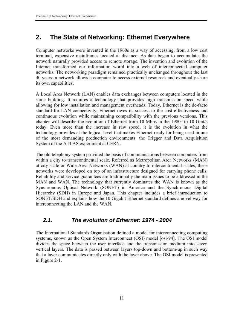
To enable this feature, a special field was added after the type/length field on the Ethernet header (Figure 2-10). The value of the type field is set to 0x8100 when the frame carries a VLAN identifier.
The 14 bits reserved to the VLAN tag identifier limited the number of VLANs that could be defined in a network to 4094. When the standard was adopted, this number was considered large enough even for the requirements of the biggest corporation. In addition to the VLAN identifier, the 802.1Q standard provided support for marking eight different classes of traffic through three bits in the VLAN tag (Figure 2-10). Different applications require different service levels from the network and Ethernet was equipped with the basic features for allowing differentiated services. However, IEEE only defined the bits while allowing the manufacturers to specify how many classes of traffic are supported by a particular device. The policies to handle this traffic were not specified by the standard. Flow control was introduced in the IEEE 802.1z standard for handling momentarily congestion on point to point full duplex links. A slow receiver could request a transmitter to pause transmission by transmitting a special Ethernet frame (Figure 2-11) that will be processed and consumed at the MAC level.
Two types of frames were defined: XOFF (stop transmit for a defined time interval) and XON (start transmit). An overloaded receiver may specify a time interval the transmitter should wait before sending the next frame. The time to wait was defined in terms of intervals equal to the time to send the minimum size frame. Also, if the processing of the backlog queue took less than anticipated, the receiving device may ask the source of traffic to resume transmission immediately by sending a XON packet. A switched Ethernet network is not allowed to contain loops. This is due to the mechanism that enables the bridge to learn what devices are attached to the network. Also, the broadcast mechanism requires a loop-free network. Since topologies became
Figure 2-10 - VLAN additions to the Ethernet frame structure
Figure 2-11 - The structure of an Ethernet flow control frame

The State of Networking: Ethernet Everywhere
21
more and more complicated, the IEEE introduced the spanning tree [bri-90] as a method of automatically detecting and removing loops from the network.
The loops are removed from the network by logically excluding the redundant connections from the packet forwarding path. Figure 2-12 presents a network where a loop was logically removed by the spanning tree. However, in case of changes in the network topology (like failure of one of the forwarding connections), the standard spanning tree algorithm was too slow to converge to an alternate topology. Since traffic was blocked while the spanning tree tried to determine a loop-free configuration, this may translate in minutes of network interruption for large complicated networks. IEEE’s response to this problem was the adoption of the 802.1w standard (Rapid Spanning Tree) that enabled faster convergence. Running only one instance of the spanning tree on devices that are part of different VLANs may hamper connectivity by removing links that would be part of a loop, but belong to different VLANs. The IEEE 802.1s standard defined multiple instances of the spanning tree running on the same bridge and in combination with the 802.1r standard enabled running one instance of the spanning tree per VLAN.
2.2. Introduction to long-haul networking technology Throughout the last 30 years, the telecommunication networks were optimized for carrying voice traffic. The digitized phone signal had a bitrate of 64 Kbps (8-bit samples taken at a frequency of 8 KHz) and it was known as Digital Signal – level 0 (DS-0). Multiple DS-0s were aggregated by multiplexers into higher order signals. The DS-1 signal, for example, contained 24 DS-0 channels. However, the hierarchy of digital signals was not standardised for rates higher than DS-3 (28 DS-1 signals) [gor-02]. In addition, the network was plesiochronous: the network devices used their own internal clocks for probing the incoming bits. The differences between free-running clocks
Figure 2-12 - Physical loop logically removed by the spanning tree

The State of Networking: Ethernet Everywhere
22
translated into bit sampling errors, hence a reduced quality of the voice signal recovered at the other end of the connection. With the start of data communications during 1970s, the telephone operators could not afford the level of bit error rates provided by a plesiochronous network. In addition, the widespread of telecommunications required worldwide-agreed standards for interconnecting equipment from different manufacturers. Introduced in the 1980’s, the SONET/SDH protocols are the foundation of today’s long haul networks. Bellcore (now Telcordia) proposed the SONET standard to the American National Standards Institute (ANSI) in 1985. In 1988, the Consultative Committee for International Telegraph and Telephone (CCITT – now ITU-T, the International Telecommunications Union) adopted SDH, a standard that includes SONET but supports different start payloads adapted to the European and Japanese telephone systems. The SONET/SDH protocols operate at layer one of the OSI stack. They allow mixing voice and data traffic while offering specific guarantees for each type of traffic. The philosophy of the SONET/SDH protocols can be summarized as follows: • Time-division multiplexed system with synchronous operation • The network is organised hierarchically, starting with slower connections at the edge followed by increasing speeds, in fixed increments, on the links towards the core • Management and maintenance functionalities are included in the communication protocol • The network supports rapid self-healing capabilities (less than 50 milliseconds) in case of an outage on a connection in a ring topology The SONET/SDH protocol was developed to support the legacy plesiochronous network hierarchy. The equipment always transmits 8000 frames per second. However, the size of the frame increased with the capacity of the channel. The current state-of-the art transmission speed is 9.95 Gbaud/s (OC-192/SDH-64). Table 1-1 shows the SONET/SDH transport hierarchy (DS – Digital Signal, STS – Synchronous Transport Signal, OC – Optical Carrier, STM – Synchronous Transport Module). Bit rate [Mbps] PDH America PDH Europe SONET SDH 9952 STS/OC-192 STM-64 2488 STS/OC-48 STM-16 622 STS/OC-12 STM-4 155 STS/OC-3 STM-1 140 E4 51 STS/OC-1 45 DS-3/T3 STS-1 SPE STS-1 SPE 34 E3 8 E2 6 DS-2/T2 2 E1 1.5 DS-1/T1 0.064 DS-0/T0 E0
Table 2-2 - The SONET/SDH hierarchy

The State of Networking: Ethernet Everywhere
23
The transmission medium for SONET/SDH is the optical fibre for long-distance communications or electrical wires for very short distances, mainly inside a rack of equipment. Due to the attenuation on the fibre, repeaters have to be installed at fixed distances on a long-distance connection. The repeaters are optical amplifiers that amplify the incoming light with no knowledge on the communication protocol. They are hence signal-agnostic. For the fibre commonly deployed (category C as defined by the ITU-T G.652 standard), the distance between two consecutive repeaters is about 40km. The repeaters are commonly referred as Erbium Doped-Fibre Amplifiers (EDFAs) from the technology employed in their construction. The EDFAs have a usable bandwidth of 30nm, centred on the 1545 nm wavelength. Within this narrow interval, they can amplify multiple optical channels. Especially at high transmission speeds, optical signal dispersion in the optical fibre is the parameter that limits the distance that can be achieved before the signal must be regenerated. The operations to be applied to the signal are reshaping, reamplification and retiming (3R regeneration). The retiming operation requires an optical-electro-optical (OEO) conversion has to be performed. Due to the electrical stage involved, the 3R regeneration stage is no longer signal-agnostic: it requires knowledge about the bitrate and generic content of the signal to be reconstructed. The 3R regenerators deployed today in the long-distance network infrastructure assume SONET/SDH framing for the incoming signal. The distance between two regenerators is in general around 600 km. The transmission capacity of an optical fibre can be increased through a wavelength division multiplex (WDM) technique that combines multiple communication channels using different frequencies over a single fibre. Up to 128 channels have been demonstrated, at a speed of 10 Gbit/s per channel, using a dense WDM technique [luc-02]. The WDM systems are signal agnostic, but whenever 3R regeneration is needed an OEO conversion has to be employed. Therefore SONET/SDH framing is required today for any signal that traverses a WDM connection. Practically, all current long-distance networks are built using SONET/SDH running over DWDM.
2.3. The 10 Gigabit Ethernet standard The 10 GE standard (IEEE 802.3ae-2002, [10ge-02]) defined the first Ethernet that did not support half duplex communications via CSMA/CD. By supporting only full-duplex connectivity, the 10 GE freed Ethernet of the CSMA/CD legacy. Henceforth, the distance of a point-to-point connection will only be limited by the optical components used for transmitting and propagating the signal. Several physical layers were defined in the 10 GE standard. The only transmission medium supported by the original version of the 802.3ae standard, issued in June 2002, was the optical fibre. The adoption of a standard for transmitting 10 GE over UTP copper cable is currently scheduled for 2006.

The State of Networking: Ethernet Everywhere
24
The standard defined a maximum reach of 40 km for a point-to-point connection, using 1550 nm lasers over single mode carrier-grade optical fibre. Two categories of physical layer devices (referred as transceivers later in this work) were supported by 10 GE: LAN PHY and WAN PHY (Figure 2-13).
LAN PHY was developed as a linear evolution in the purest Ethernet tradition: faster and further, keeping the Ethernet framing of the signal. WAN PHY was defined by IEEE for SONET/SDH compatible signalling rate and framing in order to enable the attachment of Ethernet to the existing base of long-distance network infrastructure.
2.3.1. The 10 GE LAN PHY – connectivity for LAN and MAN
The LAN PHY specified a transmission rate of 10.3125 Gbaud/s. The outgoing signal is encoded using a 64B/66B code, hence the actual transmission rate from the user’s point of view is exactly 10 Gbit/s. The original commitment of the standard, transmit 10 times more data than the previous Ethernet version, had thus been fulfilled. The minimum and maximum frame sizes of the original Ethernet have been maintained, assuring the compatibility with older versions of the standard. The structure of the frame remained unchanged as well. Four different optical devices were defined by the standard (Figure 2-13):
• the 10 GBASE-LX4, for operation over singlemode fibre using four parallel wavelengths simultaneously in order to reduce the signalling rate
• the 10 GBASE-SR, for operation over multimode fibre and a reach of up to 850 meters
• the 10 GBASE-LR, for operation over singlemode fibre and a reach of up to 10 km
Media Access Control (MAC)Media Access Control (MAC)
10 Gigabit Media Independent Interface (XGMII)10 Gigabit Media Independent Interface (XGMII)10 Gigabit Media Independent Interface (XGMII)oror
10 Gigabit Attachment Unit Interface (XAUI)10 Gigabit Attachment Unit Interface (XAUI)10 Gigabit Attachment Unit Interface (XAUI)
WAN PHYWAN PHYWAN PHY
--EWEW--LWLW--SWSW
10GBASE-10GBASE-LAN PHYLAN PHYLAN PHY
--SRSR --LRLR --ERER--LX4LX4
10GBASE-10GBASE-CWDM
Media Access Control (MAC)Media Access Control (MAC)
10 Gigabit Media Independent Interface (XGMII)10 Gigabit Media Independent Interface (XGMII)10 Gigabit Media Independent Interface (XGMII)oror
10 Gigabit Attachment Unit Interface (XAUI)10 Gigabit Attachment Unit Interface (XAUI)10 Gigabit Attachment Unit Interface (XAUI)
WAN PHYWAN PHYWAN PHY
--EWEW--LWLW--SWSW
10GBASE-10GBASE-WAN PHYWAN PHYWAN PHY
--EWEW--LWLW--SWSW
10GBASE-10GBASE-LAN PHYLAN PHYLAN PHY
--SRSR --LRLR --ERER--LX4LX4
10GBASE-10GBASE-CWDM
LAN PHYLAN PHYLAN PHY
--SRSR --LRLR --ERER--LX4LX4
10GBASE-10GBASE-CWDM
Figure 2-13- Transceiver options in the 10 GE standard

The State of Networking: Ethernet Everywhere
25
• the 10 GBASE-SR, for operation over singlemode fibre and a reach of up to 40 km
The first generation of optical devices employed by the manufacturers were modules inherited from SONET/SDH. The second generation introduced modular hot-pluggable optical devices that complied to the XENPAK [xenpak] multi-source agreement between component manufacturers. The XENPAK device implemented the Physical Medium Attachment (PMA) and Physical Medium Dependent (PMD) layers of the 10 GE specification, thus being more than pure optical equipment. The XENPAK modules were relatively large and the heat produced posed problems to certain chassis designs or network environments. Subsequent generations, the XPAK and X2 modules, featured the same optical characteristics in a reduced package while also reducing the heat dissipation. The XFP modules [xfp] only contained the PMD layer, thus further reducing the footprint, power consumption and heat dissipation. An innovative use of the 10 GE LAN PHY was demonstrated by the ESTA EU project [esta]. In two subsequent experiments, the span of a point-to-point 10 GE connection over dark fibre was pushed from 40 km (as defined by the standard) to 250 km and later to 525 km [pet-04]. This demonstration proved that a network built with 10 GE technology can span a country of the size of Denmark, almost reaching the limit where optical signals have to be regenerated. Above a certain number of amplifiers and a certain distance on the optical fibre, the optical signal needs to be fully regenerated before being transmitted towards its destination. In order to follow the traditional 10x increase in data speed, the signalling rate of LAN PHY is 10.31 GBaud due to the 64B/66B coding technique used for the signal. The data rate and framing made LAN PHY incompatible with the installed wide area network infrastructure, hence the requirement to use a different device for transmitting Ethernet frames at long distances. WAN PHY was introduced by IEEE as a direct gateway from the LAN into the SONET/SDH-dominated WAN.
2.3.2. The 10 GE WAN PHY – Ethernet over long-distance networks
WAN PHY was defined to be compatible with SONET/SDH in terms of signalling rate and encapsulation method. By inserting a WAN Interface Sublayer (WIS) before the PMD sublayer, the Ethernet frames are directly encapsulated onto SONET/SDH frames. WAN PHY therefore enabled the direct transport of native Ethernet frames over existing long-distance networks. However, the 10 GE standard does not guarantee strict interoperability of WAN PHY with SONET/SDH equipment due to mismatched optical and clock stability characteristics. Certain bits of the SONET/SDH management overhead were unused in the WAN PHY frame or were used with default values imposed by the standard. The SONET/SDH ring topology and 50ms restoration time were explicitly excluded from the WAN PHY specification.
The State of Networking: Ethernet Everywhere
26
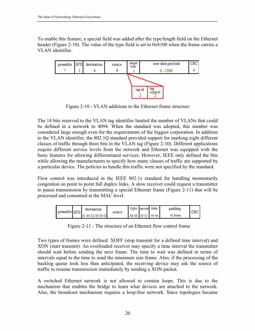
The optical jitter characteristics of WAN PHY lasers were relaxed in comparison to the SONET/SDH standard. The main reason for the relaxed jitter specifications was to provide a less expensive solution by using lower price optoelectronic devices. Although the WAN PHY standard permits timing and optics that diverge from the SONET/SDH requirements in practice there were no available components to take advantage of the opportunity. All WAN PHY implementations evaluated in this work used SONET compatible laser sources. The newly introduced XFP device format defined the same optical components to be used for SONET/SDH, 10 GE and Fibre Channel [xfp]. The clock used as a reference for WAN PHY transmissions was allowed to be less accurate (20 parts per million – ppm instead of 4.6 ppm or a variation of +/- 20 microseconds per second instead of +/- 4.6 microseconds per second of the standard SONET clock). The 20 ppm value is the required timing accuracy of a SONET/SDH connection operating in a special maintenance mode. A SONET/SDH connection operating in production mode is required to have a timing signal accuracy of 4.6 ppm or better. Instead of a direct interoperability guarantee, IEEE defined an additional piece of equipment (the Ethernet Line Terminating Equipment – ELTE) for connecting WAN PHY to SONET/SDH networks (Figure 2-14).
The main tasks of the ELTE were to compensate for differences in clock accuracy and eventually add bits in the frame management overhead. However, no manufacturer had, to date, built an ELTE. The direct attachment of WAN PHY to the existing long-distance infrastructure was the only solution available for directly connecting 10 GE equipment to long-distance networks, at the time our experiments were performed. The WAN PHY was defined to be compatible with SONET/SDH in terms of data rate and encapsulation method. The transmission rate was set to 9.95 GBaud/s, using a 64B/66B encoding. The payload capacity is only 9.58 Gbaud/s, using the Synchronous
Figure 2-14 - Native Ethernet connection to the WAN through ELTE

The State of Networking: Ethernet Everywhere
27
Transport Signal (STS)-192c / Virtual Container (VC)-4-64c frame format. This translates into a usable data rate of 9.28 Gbit/s. The theoretical Ethernet data throughput of the WAN PHY was thus only 92.94% of the throughput achieved by the LAN PHY. An automatic rate control mode was defined by the IEEE 802.3ae standard to adjust the transmission rate between the two types of PHY. There is a lot of LAN expertise and equipment readily available at research institutes and universities, but few people here have experience with SONET. The WAN PHY simplifies the implementation of the distributed LAN concept, allowing for native transmission of 10 GE frames worldwide.
2.4. Conclusion “Ethernet” is a generic denomination for the standard technology used in today’s local area networks. The current version of the Ethernet standard has greatly evolved from the original starting point. Transmitting at 10 Gbit/s and empowered by advanced features like Virtual LANs, Class of Service and Rapid Spanning Tree, Ethernet is a technology that can be used everywhere a customer is looking for cost effective solutions. The Ethernet standards define the transmission methods and specify the content of the frames. However, these standards do not include specifications related to the internal architecture of devices built for switching Ethernet frames. Chapter 3 introduces the most popular architectures of Ethernet switches.

The State of Networking: Ethernet Everywhere
28

LAN and WAN building blocks: functionality and architectural overview
29
3. LAN and WAN building blocks: functionality and architectural overview
Modern Ethernet networks are built using full-duplex links and a star architecture, with the switch at the centre of the network. The switch has two basic functions: the spatial transfer of frames from the input port to the destination port and the resolution of contention (that is providing temporary storage and perhaps a scheduling algorithm to decide the order in which multiple frames destined to the same output port will leave the switch). The switch thus acts as a statistical multiplexer, whereby unscheduled arrival frames are transferred to their destination in a predictable and controlled manner. This chapter will start with a theoretical approach to congestion through queuing theory. Then, the most common architectures used in switches will be reviewed. Traffic profiles on Ethernet networks will be briefly examined, in order to better understand the problem that switches have to address. The chapter will finish by presenting a generic Ethernet switch architecture, characteristic for the implementations present on the market in the interval 2001-2004.
3.1. Introduction to queuing theory Poisson processes are sequences of events randomly spaced in time. Poisson distributions are used for describing a diverse set of processes, ranging from natural phenomenon (the amount of photon emission by radioactive materials) to social behaviour (the arrival of clients at the cashier’s desk in a supermarket). The arrival of jobs to the service queue of a batch processing system, characteristic for the computing technology of mid-1960s, could also be described by Poisson formulas. Figure 3-1 shows a time representation of a Poisson process.
A Poisson process is characterised by a parameter noted λ that is defined as the long-time average number of events per unit time. The probability of n events to happen within a
time interval of length t is given by the formula: tn
n enttP λλ −=!)()( .
It can be shown that the number of events in disjoint time intervals are independent. The τ1, τ2, … intervals, defined as the length of the time between consecutive events, are
Figure 3-1 – Temporal representation of a Poisson process

LAN and WAN building blocks: functionality and architectural overview
30
random variables called the “interarrival times” of the Poisson process. It can also be shown that the interarrival times are independent and characterized by the probability: P(τ2 > t) = e-λt. Exponentially distributed random variables are said to be memoryless: for any t and l, P(τ > t + l | τ > l) = P(τ > t). For example, a frame arriving in a queue “knows” nothing about the arrival times of the previous frames or the state of the queue. The Poisson processes have the following two properties, of particular relevance to queuing systems:
1. The merging of two independent Poisson processes, of rate λ1 and λ2, results in another Poisson process, dependent on λ1+λ2.
2. The splitting of a Poisson process of rate λ results in two Poisson processes, characterised by pλ and (1-p)λ, where p is a uniformly-distributed random probability.
Therefore, the Poisson character of the traffic is maintained throughout a network of queues, regardless on the number of queuing stages and independent on the flow through the system. Kleinrock modelled the arrival of packets to a network queue using Poisson distributions in his seminal PhD thesis, published in 1964 [kle-61]. The assumption that incoming traffic is Poisson-distributed is widely used in modern switching theory. Figure 3-2 shows a generic queue model.
Frames arrive in the queue at a rate λ and after a processing stage they leave the queue at a rate µ. Classic queuing theory uses the Kendall notation A/S/s/k to describe a queue: - A represents the type of arrival process (examples: M – memoryless = Poisson, G –
Geometric, D – Deterministic) - S represents the time required for the processing of each frame (example: M –
exponential, D – deterministic, G – generic or arbitrary) - s is the number of servers that take frames from the queue - k stands for the capacity of the queue. For simplicity, the capacity is usually
considered infinite and the k parameter is omitted. The two types of queues most widely used for modelling switching systems are M/D/1 and M/M/1. The M/D/1 is a queue consumed by one server, has Poisson arrivals with rate λ and a deterministic service time. The M/M/1 queue is also consumed by one server, has Poisson-distributed arrival times with rate λ, but the service time is Poisson-distributed with rate µ.
Figure 3-2 - Generic queue model

LAN and WAN building blocks: functionality and architectural overview
31
The behaviour of frames in an M/M/1 queue can be modelled as a continuous Markov process chain, due to the fact that the length of the queue increases and decreases depending on the frame arrival and service times. Hence a Markov analysis can be performed on the queue in order to find the distribution of waiting times and the average queue size. Figure 3-3 presents an M/M/1 queue modelled as a Markov chain.
The interarrival rate λ and the service rate µ are the labels associated to the transitions
between the Markov states. Defining µλρ = to represent the queue occupancy rate, the
average queue size can be calculated using the formula:ρ
ρ−
=1
)(QE . It follows that ρ
has to be less than 1 in order for the queue to be stable, e.g. not grow to infinity. Intuitively, it makes sense to require that the arrival rate be lower than the service rate – otherwise, the system is just oversubscribed and the queue grows continuously. The steady state probability of finding n frames in the queue is given by the equation: pn=(1-ρ)ρn. The average delay experienced by a frame in the queue is determined using
Little’s formula:λ
)()( QETE = , where T is the time spent by a frame in the queue,
including the waiting and service times. In the case of the M/M/1 queue, λµ −
=1)(TE .
Due to the constant service time, the M/D/1 queue can no longer be studied as a continuous Markov chain. However, Little’s result still holds and together with the Pollaczek-Khinchin formula (that states that the expected waiting time is proportional
with the second order moment of the service time and a factor of )1(2 ρ
λ−
) allows for
determining the average delay. The average number of frames in the queue is determined
by the following formula: ⎟⎠⎞
⎜⎝⎛ −
−=
21
1)( ρ
ρρQE . The average delay is determined by
)(2)(
λµµλ−
=TE .
As the offered load (λ) approaches the service rate (µ), it becomes clear that the average delay experienced by a frame in an M/D/1 queue is about half of what would be the result of an M/M/1 queue. The deterministic service time may be associated with fixed frame sizes, which made the M/D/1 queuing model popular for modelling ATM switches and
Figure 3-3 - M/M/1 queue represented as a Markov chain

LAN and WAN building blocks: functionality and architectural overview
32
cell-based switching fabrics. However, assuming the length of Ethernet frames in the incoming traffic is Poisson distributed, an M/M/1 queue would better reflect the average occupancy and service time.
3.2. Switch fabric architectures Independent on the actual distribution of the frame arrival times, Ethernet switches have to solve the fundamental problem of congestion. There is only one way to solve this problem, without discarding frames immediately: providing a buffer memory, where frames may be stored temporarily until the congested resource is free. The generic architecture of a switch is presented in Figure 3-4.
The combination of switching matrix and buffer memory will be referred as the “switching fabric” throughout this document. The two components of the fabric determine the performance of the switch. This section will present the most popular switching fabric architectures. The following assumptions were considered for each of the subsequent analysis of a switch. The system operates synchronously and the time is partitioned in constant intervals, equal to the time required to transmit one frame. The length of the incoming frames is considered constant. To further mark the distinction, only the term “cell”, referring to a fixed-size logical data transfer entity, will be used throughout this section. The time is considered to be partitioned in fixed size intervals, equal to the time interval needed to transmit one cell from the input port to the output port of the switch. The switch may transmit at most one cell from an input port to an output port during a time slot. One may consider that Ethernet frames arriving to such switch are split into cells of fixed size and it is the cells that are taken into account by the scheduler. The arrivals on the N input ports of the switch are governed by identical and independent (i.i.d) Bernoulli processes. Such a process is the discrete-time equivalent of the Poisson distribution presented in section 3.1. The probability that one cell will arrive at a particular input
Figure 3-4 - Generic switch architecture

LAN and WAN building blocks: functionality and architectural overview
33
during a time slot is p. Each cell is addressed to any given input with a uniform probability of 1/N, and successive cells are independent.
3.2.1. Output buffered switches and shared memory The output buffered switch architecture allows for storing frames only at the output ports of the switch. Figure 3-5 presents the generic architecture of an output buffered switch.
The switching matrix is in fact a crosspoint fabric, connecting every input port to the memory associated to each output port. Therefore, each input port may use its own private connection to immediately transfer cells to the output port’s memory. The flow of cells from an input port towards a particular output port is thus unaffected by the flows between the other ports. The transfer of cells from the input port to the output port’s memory is performed in a FIFO manner. Karol et al. demonstrate [kar-87] that such an output buffered switch can be considered a linear combination of N parallel switches, each serving one output port. Queuing is only due to the probability of simultaneous arrivals of multiple cells addressed to the same output port, e.g. queuing appears because of an inherent property of the traffic. Follows immediately that an output buffered switch architecture will always provide the smallest average delay. Furthermore, Karol demonstrates that the steady-state probabilities for the average queue occupancy converge to those of an M/D/1 queue for each of the output ports. Therefore, an output buffered switch can achieve 100% throughput using infinite buffers that employ a FIFO strategy. Since each of the input ports is independently connected to each of the output ports, the switching matrix has to provide a speedup factor of N. In practice, the implementation is made more difficult by the fact that, in addition of the large speedup factor of the switching matrix, also the buffer memory has to allow for an access rate (N+1) times higher than the transmission speed of the output port. The direct implementation of output buffered switches in real devices is thus limited by the memory access speed and
Figure 3-5 - Generic architecture of an output buffered switch

LAN and WAN building blocks: functionality and architectural overview
34
the width of the access bus. The access time of memory chips is well known not to follow the Moore’s law governing the progress of microprocessors. In the case of integrating the buffer and the switching matrix on the same chip not only the quantity of memory that can be integrated is limited, but supporting a large number of ports would translate into a technologically unfeasible large number of contact pins for the chip. Also, such chip would become a single point of failure of the system, which would be unacceptable in carrier-grade communication systems. A solution that was proposed in order to reduce the memory scaling problem was to share the buffer between the output ports. As Engbersen showed in [eng-03], the total number of N2 connections required by the classical output buffered switch architecture is over-dimensioned with respect to any traffic pattern in real networks, apart from broadcast frames arriving simultaneously at all the input ports of the switch. Figure 3-6 shows the generic architecture of a shared memory switch.
The access to the shared memory only requires 2N times the bandwidth of the incoming connections. However, at incoming traffic speeds of Gbit/s and hundreds of ports in a switch, this architecture also becomes unfeasible to implement. Engbersen also pointed out that the shared memory architecture, usually optimised for a certain cell size, would present reduced performance in the presence of traffic burstiness due to long-range dependencies or networks that operate with frames rather than cells.
3.2.2. Input buffered switches The input-buffered switches were designed for solving the scalability problems of the shared memory switches. The memory is distributed to each one of the input ports. Hence the access speed required is equal to the transmission speed of the input port. The memory can also be easily extended to relatively large per-port quantities in order to accommodate traffic burstiness. Figure 3-7 presents the generic architecture of an input buffered switch.
Figure 3-6 - Generic architecture of a shared memory switch

LAN and WAN building blocks: functionality and architectural overview
35
Solving the issue of the memory access was done at the expense of creating a new problem: the switching matrix has now to perform the spatial transportation of the cell from the input port to the output port that will transmit the cell directly with no temporary buffer. The switching matrix is usually a crossbar – an electronic version of the two-dimensional array of electro-mechanical contacts designed for use in telephony systems in the 1950s. Other switching matrices, like multi-stage switching devices, will be described later in this chapter. However, in such matrices the input ports of the switch no longer have a permanent connection to each of the output ports. Only a single input port may send one cell to an output port during a given time slot. A global scheduling algorithm is required to examine the state of the queues at the input ports and decides the configuration of the crossbar for each time slot. The problem of the scheduler may be reduced to that of finding a matching on a bipartite graph.The input and the output ports of the switch are the nodes of the graph and the cells at the head of the queue are the edges of the graph. Efficient solutions for the bipartite graph matching problem were known since 1973 when Hopcroft and Karp published an algorithm solving this problem in O(sqrt(NM))[hop-73] . However, when the problem is put in the form of a maximum matching (either maximum size matching, e.g. maximizing the number of frames transferred, or maximum weight matching, e.g. finding the match that maximizes a certain objective criteria), the most efficient known algorithms have a complexity of O(N2.5) for uniform traffic and O(N3log(N)) for non-uniform traffic [kri-99]. Even if a match may be efficiently made by an algorithm implemented in hardware, the architectural choice of distributing the buffers in one queue at every input port creates a new problem, known as “head-of-line blocking” (HOLB). This is illustrated in Figure 3-8. If M cells arrive to the switch at the same time and are destined to the same output port, only one of them can be transferred over the crossbar during a one-cell time interval. The other cells will remain at the top of the queues of their respective ports, blocking
Figure 3-7 - Generic architecture of an input buffered switch

LAN and WAN building blocks: functionality and architectural overview
36
subsequent incoming cells to be scheduled for transfer to their destination port, even if they are destined to an output port that is available.
In their seminal paper published in 1987, Karol et al. [kar-87] study the transfer rate of such an input buffered switch for i.i.d. Bernoulli traffic. They find that, for a FIFO scheduling policy of the input queues, the switch will only allow a maximum throughout of 58.6% of the transmission line rate. Dropping blocked cells immediately, instead keeping them in the buffer and employing a classic FIFO policy, would only improve the throughput to 63.2% of the line rate and that only for an offered load higher than 88.1% [kar-87]. Karol et al. assume that the crossbar operates at the same transmission speed as the input ports. This assumption makes sense, as the input and output ports may also be considered as operating at the same transmission speed. If the crossbar operates at a different speed, a buffer will be required at the output port in order to perform the rate adaptation. Charny demonstrates in her PhD thesis [cha-98] that a speedup factor of 2 inside the crossbar, coupled with a different strategy for accessing the queue and a more sophisticated scheduling technique, allows an input buffered switch to achieve 100% throughput. She proposes the “oldest cell maximal matching” algorithm for deciding which cell will be transferred over the matrix at any given time. However, Charny also showed that a speedup factor of at least 4 is required in order to provide 100% throughput for generic traffic. For large numbers of ports inside a switch, a speedup factor of 2 on the switching matrix is already difficult to implement, while a factor of 4 would make the implementation impractical. A different technique was suggested for improving the throughput, also by Karol et al., in a subsequent paper [kar-92]. They proposed the use of separate FIFO queues dedicated to each of the output ports. This technique was called “virtual output queueing”-VOQ. It is illustrated in Figure 3-9.
Figure 3-8 - Head of Line blocking

LAN and WAN building blocks: functionality and architectural overview
37
Each input port maintains a separate FIFO for every output port. Upon arrival, the cells are immediately sent to their respective FIFO, where they wait to be scheduled over the crossbar. The separate FIFO strategy solves the head of line blocking problem because it removes the potential conflict between consecutive cells. McKeown introduced the iSLIP algorithm [mck-99a] that was able to achieve 100% throughput for i.i.d. Bernoulli traffic in an input buffered VOQ switch, while still being simple enough to allow for a hardware implementation due to its O(logN) complexity. Later, McKeown et al. proposed a set of maximum weight matching algorithms [mck-99b] that achieved 100% throughput for both uniform and non-uniform traffic. Several researchers considered the effects of traffic patterns other than the standard i.i.d. Bernoulli arrivals. Li has shown [kri-99] that the throughput of a classic input-buffered switch (without VOQ) decreases monotonically with increasing burst size. The iSLIP algorithm is notoriously unstable for some cases of non-uniform traffic. Scheduling algorithms for input buffered switches are a topical research area today. The emphasis has shifted from only assuring 100% throughout to providing bounded delay guarantees as well as fairness between concurrent flows while also taking into account traffic prioritisation. A significant part of the work is concentrated towards combined input-output buffered switches, because this architectural choice is very popular with the industry.
Figure 3-9 - Virtual Output Queuing

LAN and WAN building blocks: functionality and architectural overview
38
3.2.3. Combined input-output buffered switches The combined input-output buffered switch addresses the congestion problem by allowing the switching fabric to operate at a higher speed than the output connection. Therefore, a buffering stage has to be introduced at the output ports in order to perform the rate adaptation. The generic architecture is presented in Figure 3-10.
The separate buffers at the output ports of the switch allow for solving temporary congestion, while the queuing still takes place at the input ports. Even when using a centralised scheduler, as shown in figure 3-10, is has been demonstrated that a speedup factor of 2 is enough for this architecture to perfectly match the characteristics of an output-buffered switch [sto-98], therefore providing 100% throughput and delay guarantees. Moreover, Krishna et al. introduced a scheduling algorithm, called the “lowest occupancy cell first” (LOOFA) [kri-99], which guaranteed the work-conserving property while being independent on the switch size and of the input traffic pattern. The relative simplicity and high performance of the combined input-output switches made them popular with both industry and academia. The use of a distributed scheduler and integrating small amounts of buffering inside the crossbar has been proposed for the first time by Katevenis et al. [ste-02]. Engbersen and Minkenberg presented a similar architecture for the IBM PRIZMA switching fabric chip in [eng-02].
3.2.4. Multi-stage architectures: Clos networks The idea behind multi-stage interconnects was to reduce the number of connection point, compared with the crossbar. The concept of a Clos multi-stage network was introduced by Charles Clos in 1953 [clo-53]. A Clos network is a multi-stage network having an odd number of layers, in addition to separate layers for the input and the output ports. Figure 3-11 presents the architecture of a 3-stage Clos network. Each layer is composed of relatively small crossbar switches.
Figure 3-10 - Generic architecture of a combined buffered switch

LAN and WAN building blocks: functionality and architectural overview
39
Clos proved that this network architecture would be non-blocking if m > 2n – 1. In other words, he proved that the network is non-blocking if there are twice (less one) as many crossbars in the central layer as directly connected input or output ports of the switch on each of the crossbars at the borders of the network. Thus Clos showed, for the first time, that a non-blocking interconnection can be built with less than square complexity, measured in term of the number of crosspoints. Jajszczyk et al. showed [jaj-83] that, when splitting the capacity of each link in k equal time slots, each corresponding, for example, to a time-division multiplexed circuit, and we constrain each circuit to use no more than B time slots, no circuit will be blocked as
long as ⎥⎦⎥
⎢⎣⎢
+−−
>1
2Bk
Bnkm . A generalisation of this observation for packet networks was
made by Melen and Turner [mel-89].
3.3. Characteristics of Ethernet traffic Queuing theory was developed before Ethernet networks were invented. The applications generating the traffic have also evolved in time. Today, the LANs are traversed by a complex mixture of traffic generated by web servers, file servers providing access to the NFS or AFS distributed file systems, FTP servers and interactive telnet or secure shell (ssh) sessions, instant messaging and file sharing through peer-to-peer technologies. Several empirical studies tried to determine the exact nature of the traffic through long-term measurements performed on real networks. Most of the authors of these studies agree on the fact that most of the traffic is different than Poisson. Leland et al. studied a trace comprising 4 years of traffic at Bell Labs [lel-91]. They found evidence that the actual nature of the network traffic is self-similar, e.g. bursty over a large range of time scales. LAN traffic measured over milliseconds to seconds range exhibited the same second-order statistics as the LAN traffic measured over a period of
Figure 3-11 - Generic architecture of a three-stage Clos network

LAN and WAN building blocks: functionality and architectural overview
40
minutes. This is in strong contradiction to the predictions of the Poisson traffic, whereby the burstiness only exists over very short (time-wise) intervals. Paxson and Floyd. [pax-95] studied WAN traffic traces and also found evidence of self-similarity. Other authors [cao-01], using different traffic traces, found evidence of Poisson traffic on modern long-distance networks. The study of Roughan and Veitch [rou-03] provided new evidence for long-range traffic dependencies. Field et al. [fie-01] discovered a mixture of Poisson and self similarity in traffic traces from the LAN of the computing department of the Imperial College in London. However, a complete explanation for the observed self-similarity of the network traffic has yet to be presented. Taqqu [taq-02] recognized that partial explanations are available (such as the fact that web page response data usually requires more than one Ethernet frame to be transmitted and the same applies to file transfers, for example), but a global explanation as well as a comprehensive analysis framework has yet to be developed. The conclusion is that today’s switching fabrics are designed and dimensioned, using queuing theory, for Poisson traffic that is uniformly distributed and eventually analysed for non-uniform traffic creating hot-spots. However, this model is completely different from the actual traffic observed on the networks. In addition, Ethernet networks define multicast and broadcast traffic, whereby the traffic replication must be implemented by the switch. Although studies of multicast protocol implementations exist in the context of IP protocols, none of the articles cited in the previous section offers a theoretical approach to the switch’s performance under a mixture of unicast, multicast and broadcast traffic.
3.4. Generic architecture of an Ethernet switch In section 3.3 we have seen that the actual traffic on the network does not match the assumptions of switch design theory. Very few manufacturers make available to the public a detailed description of the internal architecture of their devices. Notable exceptions were IBM (for the PRIZMA series of switching fabrics [eng-02]), Cisco (for the GSR 12000 series of routers [mck-97]) and Broadcom (for the StrataXGS family of fabrics [lau-03]). In general, the manufacturers provide whitepapers describing the architecture in some detail, but for an average user is difficult to obtain further details beyond the information in the whitepapers and datasheets. The typical architecture of a large chassis switch from the 2002-2005 generation is presented in Figure 3-12.

LAN and WAN building blocks: functionality and architectural overview
41
The functionality of the switch is partitioned between several line cards connected to the same chassis. One line card contains the switching matrix. Usually a different line card contains a switch management module. The role of the management module is to implement the control path – network control and management protocols that are too complex to be implemented in hardware and thus require software running on a CPU. The other line cards in the chassis contain the actual input and output ports of the switch. Due to the full-duplex nature of the Ethernet traffic, the same physical port of the switch may act simultaneously as both input and output port. However, the buffers allocated to the incoming and outgoing directions are either physically separated or each of them has a minimum reserved space in a shared memory chip. The architecture thus resembles that of a combined input-output buffered switch. In addition to buffer memory, each line card that houses ports contains transceivers – the devices that actually transmit and receive the frames on/from the transmission medium. Also, a chip that encapsulates the functionality of the Ethernet MAC plus simple and fast frame processing functions is associated to each of the ports. Ports serving different transmission mediums at different speeds may coexist in the same chassis. This is the essence of a modular switch – allow the customers to mix and match line cards according to their particular requirements. The main switching matrix is usually a crossbar, with or without internal memory. The frames from lower speed ports are multiplexed before entering the switching matrix. This is because of the well-known scalability issues of the crossbars: it is not sound economically to build a crossbar with hundreds of ports, but it is feasible to build one with less ports operating at higher speeds. It is also common that the matrix operates without speedup or having a small sub-unitary speedup. In addition to the main switching matrix, a local switching stage is implemented on the line card, usually at the same stage as the multiplexing.
Figure 3-12 - Generic architecture of a modern switch
LAN and WAN building blocks: functionality and architectural overview
42
Every manufacturer provides an indication of the switching capacity of their respective devices in the datasheets. However, these numbers are not determined using queuing theory analysis but instead they are a simple sum of transmission speeds of all the available ports. Sometimes the local switching capacity is also accounted for, in addition to that of the main switching matrix. Therefore, these values should only be regarded as an indication of the best-case capacity of the switching system.
3.5. Considerations on routers and routed networks We use the term “packet” to refer to a block of data transferred over the Internet using the IP protocol. In this respect, “packet” is thus a synonym for the term “datagram” employed in the definition of the IP protocol [rfc-791]. We define the router as a device that forwards packets based on “best path” selection algorithm. For selecting the best path between the source and destination points, out of all the possible paths over the network, the router examines information located in the headers corresponding to the Layers 3 and 4 of the OSI stack protocols (Figure 2-1, chapter 2). In addition to the information from the packet to be forwarded, the router may also take into account the distance (in terms of a defined cost function) between two network nodes, the traffic load on the alternative connections and the number of intermediary points between the source and destination nodes. In contrast, an Ethernet bridge only forwards frames based on the Ethernet destination address. In the context of this work, we restrict the definition of a router to the scope of the “gateway” as introduced in RFC 1009 [rfc-1009]. The gateway is defined in RFC1009 as an IP-layer router. The forwarding of packets follows the IP specification defined in RFC 791. When IP traffic is transmitted over Ethernet networks, the IP packets are encapsulated in the data field of an Ethernet frame. The original information in the Layer 2 header of the packet is removed during the forwarding process in the router, as specified in RFC 791. It should also be noted that the IP protocol does not guarantee the in-order delivery of packets. The traditional Ethernet network based on a shared transmission medium excluded the out of order delivery of frames. The generic approach to routing in computer networks is known as the path constrained routing or the multi-path constrained routing problem. These problems have both been demonstrated to be NP-complete [che-98]. Several algorithms have been proposed and implemented taken into account limited sets of criteria The Open Shortest Path First (OSPF) [rfc-2328], Intermediate System – Intermediate System (IS-IS) [rfc-1195] and Border Gateway Protocol (BGP) [rfc-1771] are the most commonly deployed over the Internet. All these algorithms are implemented on the control path of the routers, while the data path of modern routers makes use of pre-calculated routing tables for forwarding the packets to their destination.

LAN and WAN building blocks: functionality and architectural overview
43
From the architectural point of view, a modern router is identical to the generic switch architecture presented in Figure 3-12. The main differences consist in the deeper packet inspection to be implemented by the packet processing chip on the line card and the addition of routing protocols on the control path implemented on the CPU located on the management module. Therefore it is common for high-end switches to implement a subset of the router functionalities, targeted at the enterprise market. Compared to the routers targeted to a telecommunication carrier environment, the switch/routers in the enterprise typically provide lower amounts of buffer memory, less sophisticated quality of service features and fewer implementations of routing protocols. The Multi-Protocol Layer Switching (MPLS) protocol was designed as a replacement for IP-based routing in the core network of a telecommunication carrier environment. MPLS introduces a fixed-size tag in the packet between the Layer 2 and the IP header, with the aim of simplifying the packet forwarding decision over the core of a long-distance network. When MPLS is used, the router at the edge of the network has to examine the packet Layer 3 and Layer 4 headers in order to determine what label to apply to the packet. The path through the core network is determined by the label attached to the packet. Routers further down the path only examine the MPLS label in order to take the routing decision. MPLS is one of the protocols that allows for the definition of so-called Layer 2 services. Through the use of Layer 2 services, sites located remotely would appear to be on the same LAN segment, reducing the management and simplifying the network setup. The entire content of the packet (including the entire Layer 2 header) has to be forwarded over long-distance networks. The encapsulation of Ethernet frames into MPLS is defined by the so-called “Martini draft” IETF document [mar-05]. The Martini draft specifies a method for creating point-to-point Ethernet connections over routed networks. A Virtual Private LAN Service over MPLS (VPLS) is defined in an additional Internet-Draft [las-05]. The VPLS draft defines multi-point to multi-point connectivity, thus permitting for multiple sites to be part of the same logical network. A VPLS-based network describes thus an Ethernet broadcast domain that is distributed over long-distance networks.
3.6. Conclusion Ethernet switches are the main building blocks of modern LANs. Practically all the existing devices implement a store and forward architectures. Their behaviour can be mathematically described by considering them as a collection of queues and applying queuing theory models. However, such a mathematical description implies certain restrictions on the types of traffic that can be studied. The traffic observed in real networks is quite different from the assumptions of the mathematical models. The information that can be obtained from the datasheet of a switch, complemented by possible independent evaluations of the device usually provides only an estimate of the best-case performance. Taking into account as well the diversity of architectures, testing switches is required in order to determine the performance under any particular scenario,

LAN and WAN building blocks: functionality and architectural overview
44
regardless whether this scenario can be covered or not by the standard mathematical modelling.

Programmable traffic generator using commodity off-the-shelf components
45
4. Programmable traffic generator using commodity off-the-shelf components
A network traffic generator is an apparatus that inserts traffic into the network in a controlled way. Due to the fact that Ethernet links are full-duplex, a traffic generator device has to support both the send and receive functions. The traffic is defined such as to explore the behaviour of the network in a particular scenario. The effect of traversing the network is measured on the frames received at the destination. The basic statistics that can be calculated based on the received frames are throughput, frame loss and one-way latency. These statistics have been defined in chapter 3 and can be related to a single switch or to the entire network, depending on the configuration of the testbed. Traffic generators may be used for determining the raw performance of network devices. In this scenario, only traffic that is created by the generator exists in the network. A different scenario calls for the traffic generator to provide background traffic as part of investigations onto higher layer data transfer protocols. The background traffic tries to reproduce, in a controlled environment, situations that an application may have to handle when deployed in a real system. The main aim of the traffic generators presented in this chapter was to determine the performance of Ethernet switches in isolation. As discussed in chapter 3, due to the diversity of architectures, Ethernet switches may have different levels of performance that cannot be determined just by consulting the datasheet of the device. The equipment to be deployed in the data acquisition system of the ATLAS experiment has to fulfil certain criteria [sta-05b], due to the real-time constraints of the system and the particular data transfer protocols deployed. The only way to evaluate the extent to which a certain device meets the requirements is by using a traffic generator. This chapter continues with a survey of traffic generator implementations. Then two generations of traffic generators based on a Gigabit Ethernet programmable network interface card are presented. The performance of the traffic generator is analysed. The implementation of a 32-port Ethernet test system, based on this traffic generator, is presented. The extensions of the system for determining basic performance metric of long-distance networks, using both IP and IPv6 traffic, are described and analysed. Results obtained on real long-distance Ethernet connections are presented to validate the approach.
4.1. Survey of traffic generator implementations The flow of traffic sent by an Ethernet traffic generator can be characterised in terms of the content of the frames and the time interval between consecutively sent frames. The content of an Ethernet frame (detailed in chapter 2) consists in a header of fixed size and a variable user data field. The header contains the destination address, determining thus
Programmable traffic generator using commodity off-the-shelf components
46
the path taken by the frame when traversing the network. The header may also contain VLAN and priority information, further constraining the path (in the case of the VLAN tag) or determining the class of service (in the case of the priority field). The time between consecutively sent frames determines the load over a certain point-to-point connection – the smaller this time is, the higher the number of frames hence the higher load on the link. Together with the throughput, the one-way latency is one of the most important values that have to be calculated by a traffic generator. RFC 2544 defines a way to measure the latency by sending special frames that carry a mark (referred as “timestamp” further in this document), representing the moment of sending, interleaved with the regular traffic at fixed time intervals. When such a frame is received by the traffic generator, the device would apply another timestamp corresponding to the moment of arrival of the frame to the destination. The latency is calculated as the difference between the two marks (or timestamps). The result of the calculation is meaningful only if the two clocks involved in the timestamping process were synchronised with good accuracy. On Gigabit Ethernet connections, the duration in time of a minimum length frame is 512 ns. Inside a local area network, an accuracy at least in the order of the minimum transit time would be required for the computation of the latency. The ability to timestamp each frame would allow the possibility to evaluate the jitter (the variation of latency), an important parameter for certain applications. The definition of the traffic generator presented at the beginning of chapter 4 was expressed in a generic way. A particular implementation would be made in terms of an architecture having a hardware and a software component. At a minimum, the hardware part implements the physical connection to the network. The minimal functionality of the software part would be to act as a user interface, allowing basic control over the hardware’s operation. How to best distribute the remaining functionality between these two components and the efficiency of each approach is the object of the brief survey in the remaining of this section. The discussion will exclude from start the possibility of building a customised hardware system that would integrate both the control and frame generation functions in a single box. Although possible from the technical point of view (it is the solution of choice for commercial implementations of traffic generators), this approach would make no sense in terms of the costs to a university or a research institute. The generic architecture detailed below is based on PCs, a commodity item available at relatively low costs on the market today.
4.1.1. The use of PCs as traffic generators Personal computers would seem to be ideal devices for the implementation of Ethernet traffic generators. We will only consider server PCs because their architecture is optimised for handling network traffic. The configuration of a typical server PC always includes at least one Ethernet network interface card. This card can be used as the basic hardware component of the traffic generator. All the other functions could be implemented in software running on the PC, making use of standard code libraries

Programmable traffic generator using commodity off-the-shelf components
47
offered by the operating system. One example of such an implementation was presented in [sak-01]. Many software programs that fulfil the functionality of traffic generators exist in the public domain today. The de-facto standard in the field is iperf, a program written in C++ and available for multiple operating systems [iperf]. Iperf measures the available bandwidth using the UDP and TCP protocols. It also reports the delay jitter and the UDP datagram loss. Tools like udpmon [udpmon] were developed within the time interval covered by this thesis. Udpmon improves on the iperf bandwidth and one-way latency calculation, while also providing additional statistics like CPU utilisation and latency histograms. The common problem of the software approach to traffic generators is the fact that the performance is highly dependent on the hardware architecture and components of the server. The specifications for a high-end server PC at the end of the year 2000 included a Pentium III processor at a frequency around 600 MHz. The fastest PCI bus was 32 bits wide, running at a maximum of 66 MHz thus allowing a theoretical transfer bandwidth of 2.112 Gbit/s. The performance of such computer as a traffic generator was extensively studied [gol-04, sak-01] and found to be less than satisfactory at Gigabit Ethernet speeds. In addition to the low throughput obtained, the frame timestamping operation has an accuracy in the order of 10 µs. This is caused by a combination of timing uncertainty when reading the clock register of the CPU and the accuracy of synchronization between several CPU clocks [sak-01]. In short, a PC equipped with a Gigabit Ethernet card does not fulfil the requirements to be used as a high-performance traffic generator. Similar problems were depicted by studies that took place in 2004. Backed by the latest generation Intel Xeon processors and PCI-X bus (64 bits, 133 MHz) and networking stack implemented in the 2.6 series of the Linux kernel, the performance improved but is yet not high enough for achieving full-duplex Gigabit line speed at all frame sizes [rhj-04]. The computers based on architectures for Intel Itanium-2 processors may provide the required level of performance [hur-04], but the high cost of such configuration would make building a system with tens of ports prohibitive. These systems were not available at the time of start of the work described here. The limitations of the all-software implementation of a traffic generator may be addressed by off-loading the frame generation task to an extension card, connected on the PCI bus. The advantage of this solution is the fact that no frames would be passed through the PCI bus to the server – they would have to be produced and consumed on the card. The control and user interaction components remain implemented in software, running on the PC. The extension card will have to incorporate the physical Gigabit Ethernet port to transmit and receive the frames from the network. An additional advantage of using a PCI card to directly handle the Ethernet frames would be that a single server could host multiple cards, thus becoming a multi-Gigabit traffic generator.

Programmable traffic generator using commodity off-the-shelf components
48
4.1.2. FPGA-based traffic generators The Field-Programmable Gate Arrays (FPGAs) are chips that contain basic logic blocks which can be interconnected in different configurations by a user-defined program. The program can be developed either using hardware description languages like VHDL or programming languages with C-like syntax like Handel-C. Compared to an ASIC, the FPGA allows for a faster time to market and facilitates the implementation of new features. It is worth noting that one of the first Gigabit Ethernet network adapters, the Farallon PN9000-SX, was built around an FPGA. The PCI board for traffic generator functionality would contain at least the Gigabit Ethernet PHY chip, an FPGA and maybe some memory. The functionality required for generating Ethernet frames would be implemented in the FPGA, together with the gathering of statistics on the incoming and outgoing traffic. The inherent parallelism of processing different parts of an Ethernet frame at the same time can be well exploited by the FPGA, where multiple internal blocks may access and process parts of the frame at the same time. The design and production of a customised PCI card carries a certain cost. Extensive expertise in hardware design and programming would be required. One example in this direction would be the GETB traffic generator, developed at CERN in 2004 [cio-05]. The main reason for developing this adapter was the unavailability of commodity-off-the-shelf programmable Gigabit Ethernet NICs.
4.1.3. The use of a programmable Gigabit Ethernet NIC Standard network adapters are built around an ASIC chip that integrates the Gigabit Ethernet MAC functionality and limited frame processing capabilities. The ASIC is optimised for sending and receiving frames, but extending the functionality requires a re-spin of the chip. We define a programmable NIC to be a network adapter that uses an on-board microcontroller (or microprocessor or network processor) to perform certain frame processing tasks. Firmware running on the microcontroller would implement the frame handling operations, thus allowing additional functionality to be provided by modifying the source code. A Gigabit Ethernet NIC (known as “AceNIC”) based on a programmable controller was developed by Alteon Websystems in 1999. The company made available the source code of the firmware running on the controller, together with a complete documentation in 2000. The development kit was available free of charge to anyone that purchased the NIC. The availability of free software, combined with the rights to modify the firmware and use the modified version without paying royalties were powerful arguments in favour of re-programming this network adapter to act as a traffic generator. This was the approach taken at CERN in the framework of the EU project SWIFT [swift].
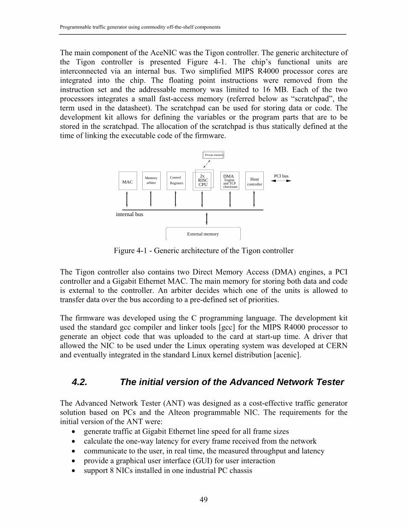
Programmable traffic generator using commodity off-the-shelf components
49
The main component of the AceNIC was the Tigon controller. The generic architecture of the Tigon controller is presented Figure 4-1. The chip’s functional units are interconnected via an internal bus. Two simplified MIPS R4000 processor cores are integrated into the chip. The floating point instructions were removed from the instruction set and the addressable memory was limited to 16 MB. Each of the two processors integrates a small fast-access memory (referred below as “scratchpad”, the term used in the datasheet). The scratchpad can be used for storing data or code. The development kit allows for defining the variables or the program parts that are to be stored in the scratchpad. The allocation of the scratchpad is thus statically defined at the time of linking the executable code of the firmware.
The Tigon controller also contains two Direct Memory Access (DMA) engines, a PCI controller and a Gigabit Ethernet MAC. The main memory for storing both data and code is external to the controller. An arbiter decides which one of the units is allowed to transfer data over the bus according to a pre-defined set of priorities. The firmware was developed using the C programming language. The development kit used the standard gcc compiler and linker tools [gcc] for the MIPS R4000 processor to generate an object code that was uploaded to the card at start-up time. A driver that allowed the NIC to be used under the Linux operating system was developed at CERN and eventually integrated in the standard Linux kernel distribution [acenic].
4.2. The initial version of the Advanced Network Tester The Advanced Network Tester (ANT) was designed as a cost-effective traffic generator solution based on PCs and the Alteon programmable NIC. The requirements for the initial version of the ANT were:
• generate traffic at Gigabit Ethernet line speed for all frame sizes • calculate the one-way latency for every frame received from the network • communicate to the user, in real time, the measured throughput and latency • provide a graphical user interface (GUI) for user interaction • support 8 NICs installed in one industrial PC chassis
Figure 4-1 - Generic architecture of the Tigon controller
PCI bus
CPU
2xRISC
Private memory
Control
RegistersMACDMAEngine
checksumand TCP
internal bus
Memoryarbiter controller
Host
External memory

Programmable traffic generator using commodity off-the-shelf components
50
The generic architecture of the ANT is presented in Figure 4-2. In addition to the PC equipped with Alteon NICs, a custom-made PCI board had to be employed. This board, based on an FPGA, was used as a high-definition common clock reference for the NICs. The clock card (as it will be referred to onwards) enabled the precise synchronisation of the timestamping processes running on the Tigon controllers. Therefore, the one-way latency computation could be performed on frames received by any of the NICs, independent on where the frame originated. See section 4.2.2 for a detailed discussion on the use of the clock card.
The software part of the ANT was composed of two drivers to allow accessing the NIC and the clock card from the Linux operating system and a GUI to interact with the user. The GUI used the Application Programmer Interface (API) of the NIC driver to pass commands and read the basic statistics computed by the firmware. The driver of the clock card programmed the FPGA on the card and provided access to registers in the FPGA to the operating system. The firmware was programmed to communicate directly with the clock card through the PCI bus of the host, with no intervention from the host processor. The ANT system was developed by a small team with whom I started as a member and later led the further technical design and development. The contributions of the other team members will be acknowledged in due place. Two pattern generators were used throughout the lifetime of the ANT. The pattern generator used in this version of ANT was developed by Stefan Haas and Frank Saka. A new pattern generator, with increased functionality, was developed by Matei Ciobotaru [cio-02] for a subsequent version of the ANT.
4.2.1. A new driver for the AceNIC card The device driver is a software component that makes a physical device available to an operating system. In the case of the Linux operating system, the device drivers are known
Figure 4-2 - The generic architecture of the initial ANT

Programmable traffic generator using commodity off-the-shelf components
51
as “modules”. With respect to the OSI stack (as presented in Figure 2-1, chapter 2), the driver of an Ethernet card implements the interface between Layer 2 and Layer 3 of the stack. The standard AceNIC driver was thus specialised in sending and receiving Ethernet frames between the NIC and the operating system of the host server. Our solution called for generating the frames directly on the NIC, therefore the bulk of functionality offered by the standard driver was not needed. The memory installed on the AceNIC can be directly accessed by the host PC over the PCI bus through a sliding window mechanism [tig-97]. In addition to the external memory window, a number of registers of the Tigon controller are exposed within the PCI-addressable range, hence could be directly accessed from the host. The standard driver used these registers in order to control the operation of the adapter. To function as a traffic generator, the AceNIC worked under the control of the host. The control software would have to be able to read the statistics from pre-defined memory locations. A simple device driver that exploited the PCI interface of the Tigon to access the external memory and the control registers could thus be developed in response to the limited set of requirements. The Linux operating system defined two types of generic devices that could be used for accessing the memory on the AceNIC: character devices and block devices. The block devices were more performance oriented and are used in general for access to storage media. The character devices were less performance-oriented and had an easier programming interface. Our intent in developing the ANT was to keep the interaction between the control software and the Tigon as low as possible. The performance of the Tigon memory access from the host was thus less important for the development of the traffic generator. Therefore the implementation of the new AceNIC driver as a character device driver was preferred. Jamie Lokier participated in the initial stages of the development. The driver, that we called “tigon” in order to differentiate it from the standard “acenic” driver, was tested on Linux kernels from the 2.2 and 2.4 series. It provided read and write memory access primitives as well as ioctl() function calls to control the operation of the adapter.
4.2.2. A new firmware running on the AceNIC The firmware supplied by Alteon with the AceNIC was optimised for exchanging frames with the host PC. The functionality required by the traffic generator was quite different – starting with the fact that the frames would be created and consumed in the NIC. Practically, the firmware was re-written from zero, with the notable exception of the parts involved in the initialization of the controller that were kept unchanged. Kevin Vella wrote the first trimmed-down transmit function and Jamie Lokier contributed an initial example of simple send and receive functions. These examples served me as a baseline for writing the optimised send and receive functions.

Programmable traffic generator using commodity off-the-shelf components
52
As detailed later in section 4.3, the two MIPS processors running at 88 MHz of the Tigon were found to be too slow for generating Ethernet frames at full Gigabit line speed. Therefore, several versions of the send and receive functions had to be developed, optimised for different operating scenarios. The optimised function for a particular scenario was copied to the scratchpad at runtime in order to speed-up the execution. A special operating mode, which we called the “warp mode” allowed for generating traffic at line speed for all frame sizes while still gathering a limited amount of statistics. The user-defined traffic pattern was controlled through a set of traffic descriptors. The descriptors were uploaded to the NIC by the host, prior to starting a measurement trial. The traffic descriptors were organised as a list and contained a valid Ethernet header for each frame, the size of the frame and the time between two consecutively sent frames. No IP or higher layer protocol header were included as the system was aimed at characterizing Ethernet switches. Different traffic profiles could be obtained by varying the inter-frame time. For example, Constant Bit Rate (CBR) traffic was obtained through a fixed inter-packet time coupled with a fixed frame size. Poisson traffic was generated using a negative exponentially-distributed random inter-frame time. The calculation of one-way latency traffic for any traffic scenario required the synchronisation of the clocks used by different cards in the timestamping process. The Tigon had a free-running clock based on an 88 MHz oscillator. The clock was implemented as a 32 bit self-incrementing register. Naturally, this clock could be used for timestamping the incoming and outgoing frames as long as all the free-running clocks in the system could be somehow synchronised to a reference value. The latency could be computed directly by the AceNIC if all the clocks in the system would start counting at the same time. The self-incrementing register could only be read but not written by the firmware. Hence the free-running clocks could not be made to start at the same time. The solution, initially designed together with Jamie Lokier, was to create a software clock on the Tigon. The software clock could be reset at the time by the firmware. It was derived from the local clock of the Tigon under the control of a global reference, available to all the NICs in the system. The clock card mentioned in Figure 4-2 provided the global reference. The clock card was developed as a traffic generator for a different network technology in the ARCHES EU-funded project [haa-98]. A master card could be connected through cables to multiple slave cards in a chain. One cable was used for carrying a reset signal, while the other cable provided a reference frequency for the slave clocks. The master card extracted its reference clock from the 66 MHz signal available on the PCI connector. Jamie Lokier wrote the code for the FPGA on the clock card and the corresponding Linux kernel module. A number of clock cards were already available, so no additional investment was required from the CERN group. The ANT system would work without the clock card, but in this case it would be unable to calculate the latency. The AceNIC was operated as a PCI master device. It could initiate a DMA transfer from the clock card located in the same chassis and thus obtain the value of the global clock reference. The local and global clocks had different counting frequencies (88 and 66

Programmable traffic generator using commodity off-the-shelf components
53
MHz, respectively). To further complicate the clock synchronisation process, the Tigon did not support floating point operations. Thus a direct mathematical translation between the two frequencies could only be implemented through emulating the division operation in firmware. This solution, implemented in assembler language and optimised by Jamie Lokier, would require about 300 clock cycles to yield a result. For reference, processing a 64 bytes frame has to be done in no more than 48 clock ticks for assuring Gigabit line speed operation. The solution to the frequency conversion problem was developed together with Jamie Lokier. We used fixed-point arithmetic and two conversion tables, stored in the fast scratchpad memory. The dimension of the tables was limited by the amount of available memory, so they could only cover intervals of about 10 ms. Therefore the tables had to be recalculated at least 100 times per second. The recalculation of the tables was coupled with a obtaining a new reference value via DMA transfer from the clock card. In order to account for possible delays in the DMA transfer (in case another device was holding the shared PCI bus), we performed this operation 128 times per second. The timestamping operation implemented through this heuristic took about 20 clock cycles (of the Tigon internal 88 MHz clock), so the total time used at the sender and at the receiver was comparable to the time budget of the Gigabit Ethernet transmission for the minimum size frame. Every outgoing frame received a 32 bits timestamp value before being added to the MAC transmit queue. The timestamp was inserted in a pre-defined position in the user data part of the Ethernet frame. Another timestamp was applied when the frame was completely received at the destination card. The one-way latency, expressed in 66 MHz clock ticks (15 ns-long) was obtained as the difference between the two timestamps. The components of the measured latency value are detailed in Figure 4-3. The 32 bit value only covered latencies less than 64.42 seconds. The free running counters would wrap around when the value 2^32 would be reached. However, such frame latencies (corresponding to almost 18 hours) were considered impossible for LANs. Thus, the timestamping process was designed such that only took into account one wrap around of the clock register. Results on the accuracy of the timestamping process are presented in the section 4.3.
Figure 4-3 - Latency measured by the ANT

Programmable traffic generator using commodity off-the-shelf components
54
The following statistics derived from the network traffic were made available by the firmware to software running on the host PC: number of sent and received frames and bytes, number of frames received with CRC errors, number of lost frames. The latency was made available as a histogram or as the sum of latencies for the frames represented in the received frames counter.
4.2.3. The Graphical User Interface The use of a GUI to control the ANT was specified in the requirements of the system. The GUI was built using the GTK 1.2 graphical library for the Linux operating system. It controlled up to eight AceNIC adapters installed in the same chassis. The code was organised in two parts: a low-level library to communicate with the NICs through the interface offered by the kernel module and a higher level part to display the results and eventual error messages. The GUI implemented basic test management functionality, together with incremental real-time control on the offered traffic load. A screenshot of the GUI used in the initial ANT system is presented in Figure 4-4.
The raw values of the counters were collected from the NICs and the throughput and corresponding frame rates were calculated by the low-level library. Results from the on-going test were displayed in real time on the dials and saved on a file for later processing. Latency histograms collected by the card were directly saved to a file.
Figure 4-4 - The GUI of the initial ANT

Programmable traffic generator using commodity off-the-shelf components
55
4.3. Results from the initial ANT The baseline performance of the send, receive and clock synchronisation functions was determined using two AceNIC adapters directly connected through an optical fibre cable. The adapters were operated in full-duplex mode, sending and receiving frames at the same time. Figure 4-5 presents the throughput measured for the standard and warp operating modes, compared to the theoretical Gigabit Ethernet line rate. The warp mode provided the maximum frame generating performance, filling all the available bandwidth.
The frame generation performance in the standard operating mode was reduced for small frame size, due to the overhead introduced by the computation of latency and additional per-frame statistics on the traffic (like the frame loss, for example). The maximum frame processing rate attained in the standard operating mode is about 806000 frames per second (counting the frames sent and received in full-duplex mode). The sending and the receiving of frames were implemented as software processes. Each of them ran on a separate processor of the Tigon. An event was triggered by hardware on the receive processor when the frame was received completely by the adapter and the CRC was validated by the MAC. In the interval between analysing the received frames, the processor waited for events in a tight loop polling the event register. The processor that ran the send code also performed the table computation associated to clock synchronisation. It waited in a tight loop checking the event register for a timer interrupt (associated to a clock synchronization event) or for the moment to add the next frame to the MAC send queue. Certain registers that had to be accessed in this process were located in the main memory of the NIC, hence the processors had to compete for bus access. The default setting was for the processors to have the lowest priority when accessing the memory. The MAC and the DMA engines had higher priority. This was done in order to guarantee that no Ethernet frames will be dropped by the MAC or by the DMA engines. The memory access time for a processor depended on the amount of network traffic, but also on the activity of the other processor.
Figure 4-5 – The performance of the ANT send and receive functions
0
200000
400000
600000
800000
1000000
1200000
1400000
1600000
64 128
256
384
512
640
768
896
1024
1152
1280
1408
1518
Frame size [bytes]
Rece
ived
thro
ughp
ut [f
ram
es/s
]
standardwarptheoretical

Programmable traffic generator using commodity off-the-shelf components
56
Figure 4-6 presents the average latency measured on a direct connection between two AceNICs. The average is calculated for an interval of 1 second. A constant overhead of about 1.63 µs is introduced by the frame send and receive processes. The latency was measured at an offered load of 10% of the line rate.
Figure 4-7 shows a histogram of the latency values measured for three frame sizes, also for an offered load of 10% of the line rate using constant bitrate traffic. The latency is calculated using the 66 MHz global clock. The width of one bin of the histogram is 15 ns. The mean and variance values of the data in the histograms are presented in table 4-1. The width of the histogram peak, at half of its height, is between about 200 ns (for the 64 bytes frames) and about 300 ns (for the 1518 bytes frames). The increase in variance can be explained by the uncertainties introduced by the access to from the Tigon to the shared memory. Four main actors are competing for access: the send and receive MAC processes, the ANT send process (implemented on CPU1 of the Tigon) and the ANT receive process (implemented on CPU0 of the Tigon).
0
2
4
6
8
10
12
14
16
64 128
256
384
512
640
768
896
1024
1152
1280
1408
1518
Frame size [bytes]
Tim
e [u
s]
ANT latencyGigE tx time
Figure 4-6 - Average ANT latency over a direct Gigabit Ethernet connection
(a) 64 bytes
Figure 4-7 - Latency on a direct connection, 1518 bytes
0.8 1 1.2 1.4 1.6 1.8 2 2.2 2.4 2.60
1
2
3
4
5
6
7
8
x 105
Latency [us]
Nu
mb
er
of
fra
me
s
4.5 5 5.5 6 6.5
0
1
2
3
4
5
6
7
8
x 104
Latency [us]
Num
ber
of fr
am
es
12.6 12.8 13 13.2 13.4 13.6 13.8 14 14.2 14.40
0.5
1
1.5
2
2.5
3
3.5
x 104
Latency [us]
Num
ber
of fr
am
es
(b) 512 bytes (c) 1518 bytes

Programmable traffic generator using commodity off-the-shelf components
57
Table 4-1 - Statistical parameters calculated from the histograms in Figure 4-7
Figure 4-8 displays the latency histograms for two frame sizes, measured on 100000000 frames at an average load of 50% and for the maximum load achievable for that particular frame size. Constant bitrate traffic was used in theses trials.
Figure 4-9 presents the histograms of the time intervals between consecutive frames arriving at the receiver, for constant bitrate traffic. The interval between consecutive frames is calculated from the start of one frame to the start of the next frame. The inter-arrival time is calculated using the internal clock of the Tigon (88 MHz), therefore the width of a bin is 11.3 ns.
Frame size [bytes] Mean [µs] Variance 64 1.725 0.0850
512 5.350 0.6629 1518 13.375 2.8175
4.8 5 5.2 5.4 5.6 5.8 60
1
2
3
4
5
6
7
x 106
Latency [us]
Num
ber
of fr
ames
12.8 13 13.2 13.4 13.6 13.8 14 14.20
0.5
1
1.5
2
2.5
3
3.5
4
4.5
5
x 106
Latency [us]
Num
ber
of fr
ames
4.8 5 5.2 5.4 5.6 5.8 60
1
2
3
4
5
6
7
x 106
Latency [us]
Num
ber
of fr
ames
12.8 13 13.2 13.4 13.6 13.8 14 14.20
1
2
3
4
5
6
x 106
Latency [us]
Num
ber
of fr
ames
512 bytes 50% load Mean: 5.325µs Variance 0.0791
512 bytes 99% load Mean: 5.396µs Variance 0.0684
1518 bytes 50% load Mean: 13.394µs Variance 0.1996
1518 bytes 100% load Mean: 13.443µs Variance 0.2002
Figure 4-8 - Latency distribution on a direct connection

Programmable traffic generator using commodity off-the-shelf components
58
The graph shown in Figure 4-9(b) exposes the fact that the 100% load reported by the ANT in the case of the standard firmware actually includes a rounding error. The actual throughput is 99.6% of the line rate. The smaller bins in the histogram account for the difference in load. Figure 4-10 presents the inter-packet arrival time for a Poisson distributed traffic. An average offered load of 50% of the line speed was generated using 1518 bytes frames.
The negative exponential distribution that characterises the Poisson traffic can be still observed in the histogram. The structure in the histogram is caused by the fact that the traffic descriptors used discrete inter-frame times, with a resolution of 1 us.
(a) 50% load (b) 100 % load
Figure 4-9 - Inter-arrival time histograms for 1518 bytes frames
Figure 4-10 - Inter-arrival time for Poisson traffic

Programmable traffic generator using commodity off-the-shelf components
59
We can conclude that the ANT fulfilled all the initial requirements in terms of performance of the traffic generation function and computation of the latency. Further discussion on the ANT performance can be found in [swi-01] and [dob-02]. However, the tester was limited to single chassis housing up to 8 ports. Support for IP traffic was required for the investigations on the use of long-distance connections over the Internet in the context of the studies related to the real-time use of computing farms in the TDAQ system. A second generation of the ANT was developed to answer these new requirements.
4.4. The distributed version of the ANT The second version of the ANT was developed in 2002. The new system was designed such that it could be scaled up to 256 devices, with nodes that could be distributed anywhere in the world under the control of a unique user interface. The generic architecture of the distributed ANT is presented in Figure 4-11.
The main issue to be addressed by the distributed ANT version was to provide a generic mechanism for clock synchronization of the traffic generator NICs. The synchronisation of computers located in the same laboratory could be addressed by the master-slave mechanism already present in the clock cards. Computers situated in geographically remote locations required a global time reference to be supplied. This reference was provided by using signals from the Global Positioning System (GPS). One additional PCI card, available as commodity item on the market, was required at every location for receiving the GPS signals. The new method for clock synchronisation is presented in more detail in section 4.4.1. The low-level library and high-level software code from the old GUI were evolved in two separate components of the new ANT. The low-level library that directly accessed the
Figure 4-11 - The generic architecture of the distributed ANT

Programmable traffic generator using commodity off-the-shelf components
60
Linux kernel module interface evolved into a component known as the “Agent”, a server program that ran on every computer part of the testbed. The high-level software code of the initial GUI was re-written from the ground up as a client for the Agent. The new GUI communicated with the Agent through the standard Linux network sockets interface using the TCP/IP protocol to transport statistics data and control messages. Therefore, the new GUI could control computers located anywhere in the world. The distributed ANT system was also the result of team work, as was the previous version. I was responsible for the design and implementation of the client-server components and contributed to the development of the other parts of the system. The GUI could integrate up to 256 network interface cards. Due to cost issues and the unavailability of Alteon AceNIC cards starting at the end of 2002, the maximum number of ports that were actually used in the system was 32. Figure 4-12 shows the distributed ANT GUI in operation controlling a 32-port Gigabit Ethernet traffic generator system.
The offered load, received throughput and average latency were displayed in real-time on the GUI. A Windows wizard-like interface was developed for guiding the user through the test definition process. The firmware running on the AceNIC required no modifications for operating in a distributed environment, as long as the test scenario only required Ethernet traffic. The experience accumulated while using the old version dictated small feature additions, like separating the frame counters for all eight traffic priorities defined in the IEEE 802.1q standard and per-source calculation of the frame loss for up to 32 traffic sources. Major developments at the firmware level were required for the characterisation of long-distance network connections over the Internet.
Figure 4-12 - A 32-port system controlled by the distributed ANT GUI
Programmable traffic generator using commodity off-the-shelf components
61
4.4.1. Clock synchronisation for the distributed ANT The computation of the one-way latency requires the timestamping processes of the transmitter and the receiver to be synchronised to the same clock reference. In LANs, the latency may be approximated by calculating the round trip time of a frame and dividing this value by two. However, on long-distance networks, the return path of the frame may be different from the departure path therefore the latency of each of the paths cannot be estimated using the round trip time. The clock cards of the computers that composed a locally distributed ANT could be interconnected through coaxial cables. The master clock card would thus provide a clock reference to slave cards installed in other computers. The slave clock cards would in turn propagate the reference to the NICs installed in the same chassis. However, such a direct hardware connection could not be implemented in the case of a geographically distributed system. The GPS is based on a constellation of satellites placed on fixed orbits. The satellites continuously transmit their position and a timestamp value of the Coordinated Universal Time (UTC). The satellites are equipped with atomic clocks, hence the accuracy of the timestamp is in the range of nanoseconds. A GPS receiver located on the surface of the Earth can use a triangulation method, using signals from several satellites, to calculate its position within several tens of meters. Using the timestamps emitted by the satellites, the receiver can also synchronize an internal clock to the UTC with accuracy in the range of 100 ns [mfg-02]. GPS receivers with a PCI bus interface were available as commodity items on the market. Unfortunately, none of the available models could support a direct DMA transfer of the type required for the synchronisation of the AceNIC timestamping function. The solution, designed together with Brian Martin and Stefan Haas, was to take advantage of signals that were available through serial connectors of the Meinberg GPS167PCI card [mfg-02]. A high frequency signal of 10 MHz and a 1 Hz pulse were accessible on two separate pins of the serial output connector. The 10 MHz signal used a high precision internal oscillator as reference. The internal oscillator was controlled by using the results of GPS timing computation [mfg-02]. The 1 Hz pulse was released as a TTL signal every time the UTC second was updated. The two signals were transmitted to the local clock card by direct coaxial cable connections. The 10 MHz signal was used by the local clock card as the input signal for its self-incrementing counter. The counter was reset to a known value each time a pulse was received on the 1 Hz signal line. The clock synchronisation solution required reprogramming the FPGA on the local clock card. Miron Brezuleanu and Matei Ciobotaru participated in the design and implemented the solution, under my supervision. The implementation included a method of synchronously resetting the counters at the same time when starting a test, described in [bre-02]. The graph shown in Figure 4-13, obtained by Miron Brezuleanu and included in [bre-02] shows the difference, in clock ticks, between the value of the counter on the clock card with respect to the reference value at every 1 Hz pulse for an interval of 256 seconds.
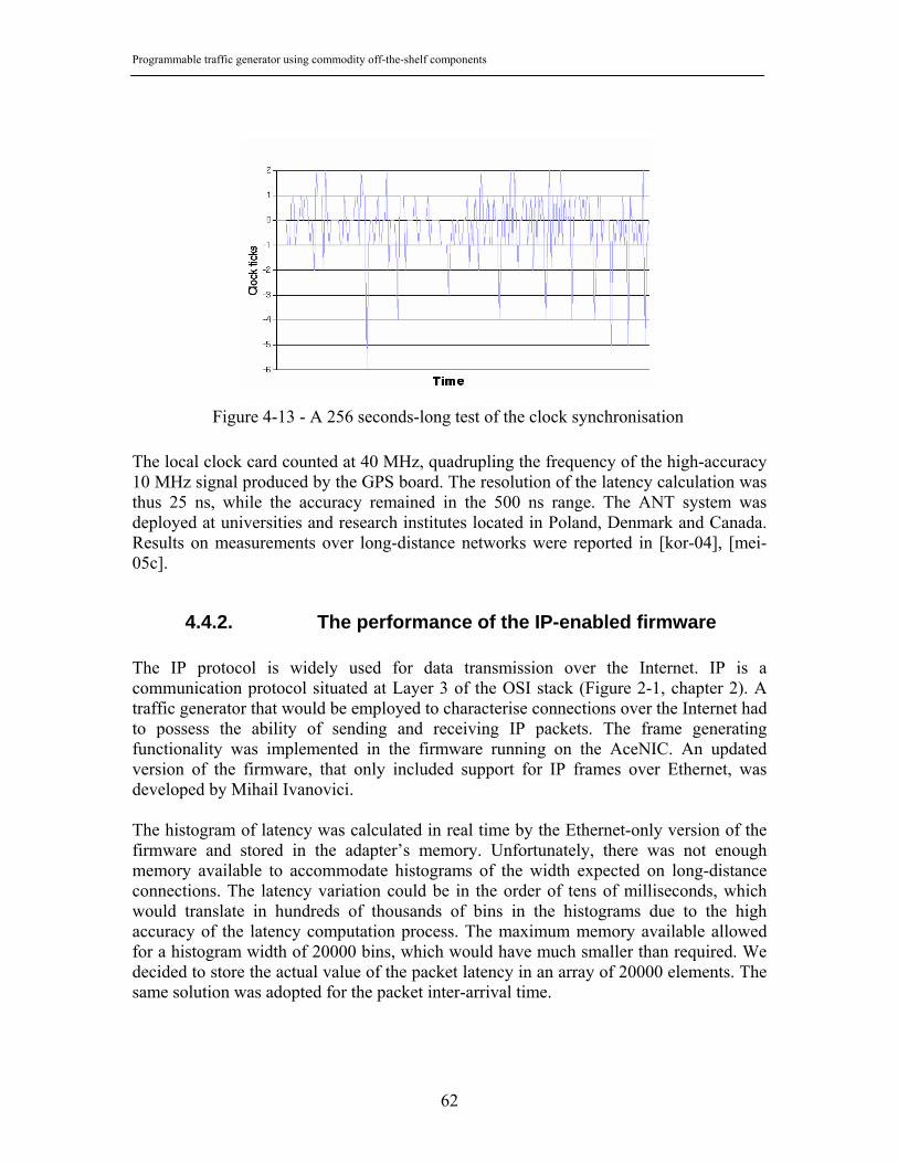
Programmable traffic generator using commodity off-the-shelf components
62
The local clock card counted at 40 MHz, quadrupling the frequency of the high-accuracy 10 MHz signal produced by the GPS board. The resolution of the latency calculation was thus 25 ns, while the accuracy remained in the 500 ns range. The ANT system was deployed at universities and research institutes located in Poland, Denmark and Canada. Results on measurements over long-distance networks were reported in [kor-04], [mei-05c].
4.4.2. The performance of the IP-enabled firmware The IP protocol is widely used for data transmission over the Internet. IP is a communication protocol situated at Layer 3 of the OSI stack (Figure 2-1, chapter 2). A traffic generator that would be employed to characterise connections over the Internet had to possess the ability of sending and receiving IP packets. The frame generating functionality was implemented in the firmware running on the AceNIC. An updated version of the firmware, that only included support for IP frames over Ethernet, was developed by Mihail Ivanovici. The histogram of latency was calculated in real time by the Ethernet-only version of the firmware and stored in the adapter’s memory. Unfortunately, there was not enough memory available to accommodate histograms of the width expected on long-distance connections. The latency variation could be in the order of tens of milliseconds, which would translate in hundreds of thousands of bins in the histograms due to the high accuracy of the latency computation process. The maximum memory available allowed for a histogram width of 20000 bins, which would have much smaller than required. We decided to store the actual value of the packet latency in an array of 20000 elements. The same solution was adopted for the packet inter-arrival time.
Figure 4-13 - A 256 seconds-long test of the clock synchronisation

Programmable traffic generator using commodity off-the-shelf components
63
Figure 4-14 presents a comparison of the histogram for the inter-arrival times on a direct connection between two AceNICs (Figure 4-14, a) and the effect of a long-distance connection (Figure 4-14, b, c). The data displayed on graphs 4-14,b and 4-14,c was collected on the two directions of the connection between Geneva, Switzerland and Krakow, Poland. The asymmetry between the two directions of the long-distance connection was expected and is due to the sharing of the available bandwidth with other users. The horizontal axis of the graphs represent the inter-arrival time in µs. The vertical axis represent the number of packets received.
The long-distance networks do not guarantee the in-order delivery of the IP packets. A counter for packets arrived out of order was implemented in the IP-enabled version of the firmware. Figure 4-15 shows the increase of frames received out of order during a measurement performed on the Geneva – Krakow connection using 1500 bytes IP frames. The offered load was 100% of the 1 Gbit/s capacity of the circuit.
(a) (b) (c)
Figure 4-14 – Packet inter-arrival times on local and long-distance connections
266 267 268 2690
1000
2000
3000
4000
Direct back−to−back connection
Frame inter−arrival time [us]240 260 280 300
0
1000
2000
3000
4000
Frame inter−arrival times [us]
Krakow − Geneva
240 260 280 3000
1000
2000
3000
4000
Frame inter−arrival time [us]
Geneva − Krakow
Figure 4-15 - Out-of-order frames on the Geneva-Krakow connection

Programmable traffic generator using commodity off-the-shelf components
64
The results presented in Figure 4-15 will be discussed further in chapter 7, in the context of the ATLAS studies for the real-time access to remote computing farms.
4.4.3. The IPv6 traffic generator The limitations of the IP protocol, in particular the limited address space and the lack of native support for secure communications, are addressed by the IPv6 protocol. Certain network operators manage IPv6 networks in parallel to the standard IP network. A demonstrator platform for IPv6 routing was developed in the context of the ESTA EU project during 2003. The demonstrator was built around a network processor capable of routing IPv6 packets internally at 10Gbit/s. The interface was in the form of 8 x 1 Gigabit Ethernet connections. The Gigabit Ethernet streams were merged together and processed internally as a single stream at 10 Gbit/s. Modifying the ANT to generate IPv6 traffic was a natural solution for validating the ESTA IPv6 reference platform. The main changes required were at the AceNIC firmware level. All the features of the Ethernet version of the ANT are available in the IPv6 version. Sent and received throughput, one-way latency and packet loss for up to 32 sources at each destination were calculated and displayed in real-time on the GUI. The control and data display interfaces of the ANT were also updated to accommodate IPv6 traffic generation.
4.5. Conclusion This chapter presented in detail the design and implementation of a 32-port Gigabit Ethernet programmable traffic generator, known as ANT. The system was built using commodity off the shelf components: industrial PC chassis and Gigabit Ethernet network interface cards. The use of custom-developed PCI cards was necessary for allowing the computation of one-way latency with a precision better than 400 ns. The system was capable of sending and receiving traffic at Gigabit Ethernet nominal line speed for all the frame sizes defined in the IEEE 802.3 standard. The traffic profiles could be controlled through user-defined descriptors uploaded to the card prior to the start of a measurement session. The system was extended to support IP and IPv6 traffic, with test stations deployed in Canada, Denmark and Poland. The one-way latency computation was possible through the addition of one GPS receiver per site. The accuracy of the latency computation process remained unchanged. Chapter 5 will describe how simple measurements performed with the ANT system allowed revealing details on the internal architecture of switches from the generation available on the market between 2001 and 2003. Chapter 7 will mention results from characterisation of the long-distance connections using the ANT.
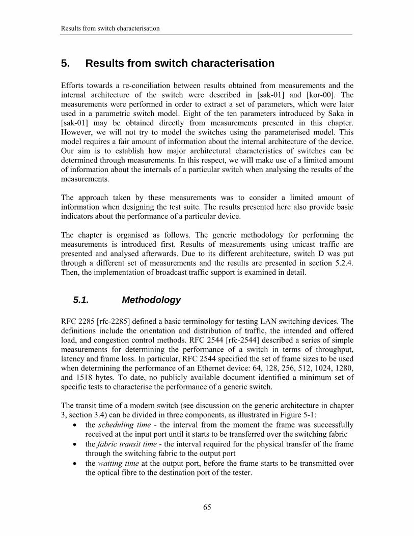
Results from switch characterisation
65
5. Results from switch characterisation Efforts towards a re-conciliation between results obtained from measurements and the internal architecture of the switch were described in [sak-01] and [kor-00]. The measurements were performed in order to extract a set of parameters, which were later used in a parametric switch model. Eight of the ten parameters introduced by Saka in [sak-01] may be obtained directly from measurements presented in this chapter. However, we will not try to model the switches using the parameterised model. This model requires a fair amount of information about the internal architecture of the device. Our aim is to establish how major architectural characteristics of switches can be determined through measurements. In this respect, we will make use of a limited amount of information about the internals of a particular switch when analysing the results of the measurements. The approach taken by these measurements was to consider a limited amount of information when designing the test suite. The results presented here also provide basic indicators about the performance of a particular device. The chapter is organised as follows. The generic methodology for performing the measurements is introduced first. Results of measurements using unicast traffic are presented and analysed afterwards. Due to its different architecture, switch D was put through a different set of measurements and the results are presented in section 5.2.4. Then, the implementation of broadcast traffic support is examined in detail.
5.1. Methodology RFC 2285 [rfc-2285] defined a basic terminology for testing LAN switching devices. The definitions include the orientation and distribution of traffic, the intended and offered load, and congestion control methods. RFC 2544 [rfc-2544] described a series of simple measurements for determining the performance of a switch in terms of throughput, latency and frame loss. In particular, RFC 2544 specified the set of frame sizes to be used when determining the performance of an Ethernet device: 64, 128, 256, 512, 1024, 1280, and 1518 bytes. To date, no publicly available document identified a minimum set of specific tests to characterise the performance of a generic switch. The transit time of a modern switch (see discussion on the generic architecture in chapter 3, section 3.4) can be divided in three components, as illustrated in Figure 5-1:
• the scheduling time - the interval from the moment the frame was successfully received at the input port until it starts to be transferred over the switching fabric
• the fabric transit time - the interval required for the physical transfer of the frame through the switching fabric to the output port
• the waiting time at the output port, before the frame starts to be transmitted over the optical fibre to the destination port of the tester.
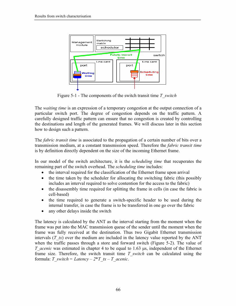
Results from switch characterisation
66
The waiting time is an expression of a temporary congestion at the output connection of a particular switch port. The degree of congestion depends on the traffic pattern. A carefully designed traffic pattern can ensure that no congestion is created by controlling the destinations and length of the generated frames. We will discuss later in this section how to design such a pattern. The fabric transit time is associated to the propagation of a certain number of bits over a transmission medium, at a constant transmission speed. Therefore the fabric transit time is by definition directly dependent on the size of the incoming Ethernet frame. In our model of the switch architecture, it is the scheduling time that recuperates the remaining part of the switch overhead. The scheduling time includes:
• the interval required for the classification of the Ethernet frame upon arrival • the time taken by the scheduler for allocating the switching fabric (this possibly
includes an interval required to solve contention for the access to the fabric) • the disassembly time required for splitting the frame in cells (in case the fabric is
cell-based) • the time required to generate a switch-specific header to be used during the
internal transfer, in case the frame is to be transferred in one go over the fabric • any other delays inside the switch
The latency is calculated by the ANT as the interval starting from the moment when the frame was put into the MAC transmission queue of the sender until the moment when the frame was fully received at the destination. Thus two Gigabit Ethernet transmission intervals (T_tx) over the medium are included in the latency value reported by the ANT when the traffic passes through a store and forward switch (Figure 5-2). The value of T_acenic was estimated in chapter 4 to be equal to 1.63 µs, independent of the Ethernet frame size. Therefore, the switch transit time T_switch can be calculated using the formula: T_switch = Latency – 2*T_tx – T_acenic.
Figure 5-1 - The components of the switch transit time T_switch

Results from switch characterisation
67
The latency is available to the user in the form of a histogram, calculated in real time by the AceNIC, or as an average value calculated by the ANT software for a pre-configured time interval. The values presented on the graphs in this chapter are those of the average latency calculated by the ANT over an interval of 1 second. The latency was recorded after a minimum interval of 60 seconds of stable operation. In view of the limitations presented in chapter 4, the latency measurements were only performed for a subset of the frame sizes specified in RFC 2544.
5.1.1. Unicast traffic All the frames sent during a measurement trial must have the same length in order to use the average latency as an estimate of the per-frame latency. It is the per-frame latency that we need for the calculation of T_switch. Taking into account the length of the frame, we could thus estimate the internal transfer speed of the switch. The use of the fixed frame size during a trial has the additional advantage to guarantee zero waiting time when no congestion is created through the traffic pattern. Two types of traffic will be used during the measurements: constant bitrate and Poisson. Both traffic types are generated with fixed-size frames. The constant bitrate traffic is composed of frames separated by equal time intervals. Figure 5-3(a) shows an idealistic representation of constant bitrate traffic. In fact, the interval between frames consecutively sent by the ANT was not constant. You are referred to chapter 4, figure 4-9 for a typical histogram of the inter-arrival times. Constant bitrate traffic sent between pairs of ports is not expected to create congestion inside the switching fabric. The latency measured by ANT for this type of traffic only reflects the network transit time of a frame. We can thus calculate T_switch, for a given frame size. Differences in the values measured for T_switch on the same device but using different traffic distributions may be translated in considerations about the internal architecture of the device.
Figure 5-2 - The components of the latency reported by ANT in a LAN test

Results from switch characterisation
68
The combination of random choice of destinations with Poisson inter-frame times implements the traffic type that is most popular in characterising switch architectures through mathematical modelling. A sequence of frames separated by Poisson intervals is represented in Figure 5-3(b). The particular patterns employed in section 5.2.3 used constant frame sizes and a uniformly distributed random choice of the destinations. The times between consecutively sent frames were generated using a negative exponential distribution. This traffic pattern creates bursts of traffic on the point-to-point connection due to the particular choice of the inter-frame times. It creates congestion inside the switch due to the uniform random distribution of the destinations. The most important value measured for the random traffic is the throughput. The latency measured in this scenario is mainly due to the queuing induced by the traffic pattern. While it may be interesting to compare, in terms of latency, how different switches handle the congestion, these values cannot give additional information regarding the switch architecture.
5.1.2. Broadcast traffic As explained in detail in chapter 3, Ethernet networks are natural broadcast-enabled environments. The broadcast was easily implemented in the original Ethernet where all the members of the network listened to the same physical transmission medium. However, in modern switched networks, the support for broadcast traffic requires transmitting the same frame out on all the active ports of the switch. Thus an incoming broadcast frame has to be replicated inside the switch. The implementation of the frame replication is proprietary to every switch manufacturer. We introduce a “normalized received load” in order to account for the amount of traffic replication that has to be performed by the switch. The normalized received load is
calculated using the following formula: inoutsspins
inoutsoutsnl_)(*_
100*)__(+−
+= , where:
nl – the normalized value of the measured received load, for all the ports in the test s_out – the sum of the received load measured on all the ports that are not sources of broadcast traffic
Figure 5-3 - Constant bitrate (a) and Poisson traffic (b)

Results from switch characterisation
69
s_inout - the sum of the received load measured on all the ports that are sources of broadcast traffic. The ports that acts as broadcast sources receive less traffic, because a switch does not forward broadcast frames out on the originating port. s_in – the total traffic load generated by the broadcast sources p – the number of ports involved in the test s – the number of broadcast sources We start characterising the switch by sending traffic within one line card. We measure the throughput and average latency and establish a mapping between the measured values and architectural features. We continue by sending traffic between different line cards in order to characterise the switching fabric.
5.2. Results from measurements using Ethernet unicast traffic
At the end of the test interval, discussions with each of the manufacturers brought more light on the actual architecture of the switches. However, the content of these interactions is covered by non-disclosure agreements. This is also the reason why the switches will be referred only as A, B, C, D and E. Table 5-1 summarises the information regarding the internal architecture of the devices that was available at the start of the tests. All switches used store and forward architectures.
switch GE ports per line card
Local switching on the line card Buffers Switch fabric
architecture
A 8 No data Input-output Crossbar
B 8 No data Input-output Crossbar
C 24 No Input-output Crossbar
D 8 some Input-output Multi-stage; static routing
E 8 No data Input-output Dual parallel
fabrics, static and dynamic routing
Table 5-1 - Summary of switch architectures under test
5.2.1. Intra-line card constant bitrate traffic The traffic was sent between pairs of ports using a one-to-one bi-directional and symmetrical mapping, as shown in Figure 5-4. The two ports in the pair were always chosen to be neighbours on the same line card. This traffic distribution can be viewed as a particular realization of the partial mesh traffic defined in RFC 2285. We will start by

Results from switch characterisation
70
discussing the throughput and will continue with a detailed analysis of the latency measured for the same traffic distribution. The graph shown in Figure 5-4 presents the received rate for all frame sizes specified in RFC 2544. Switch B has a throughput of 100% only for frame sizes larger than 66 bytes. The other switches presented a 100% throughput for this particular distribution of the traffic. The measurements were performed in the ANT warp mode, which allowed generating a load of 100% percent of the line speed while performing only a limited amount of calculations on the traffic generator.
Figure 5-5 presents the average latency measured on the received traffic for three frame sizes that allowed the tester to send and receive up to 100% of the line rate while still being able to compute the latency in real-time. No frames were lost during this test, hence the choice of the offered load (instead of the received load) for the label of the horizontal axis. Switch C presented an interesting variation of the latency with the size of the frame. It was unexpected and counter-intuitive for the average latency to vary for this distribution of the traffic. The results from switches A, B and E will be interpreted first, leaving the results of switch C for the final part of this sub-section.
0 200 400 600 800 1000 1200 1400 160090
91
92
93
94
95
96
97
98
99
100
101
Frame Size [bytes]
Rec
eive
d Lo
ad [%
]
switch Aswitch Bswitch Cswitch EOffered Load
Figure 5-4 - Intra-line card traffic distribution and throughput

Results from switch characterisation
71
Figure 5-6 presents the T_switch for switches A, B and E. The results obtained on switch C are discussed later in Figure 5-7. The value of the average latency used for calculating T_switch was taken from the dataset presented in Figure 5-5. The standard deviation of the average latency calculation was added to the data points in the form of error bars. The transmission time on a Gigabit Ethernet connection was included in the graph for comparison. A full line was used for the Gigabit Ethernet graph because the transmission time can be directly obtained, for each frame size, from the transmission rate defined by the standard. The scale of the vertical axis differs between the two graphs in order to better observe the details of the points representing switch B and E.
0 10 20 30 40 50 60 70 80 90 100 11010
20
30
40
50
60
70
Offered Load [%]
Ave
rage
Lat
ency
[us]
Switch A
512 bytes1024 bytes1518 bytes
0 10 20 30 40 50 60 70 80 90 100 11010
20
30
40
50
60
70
Offered Load [%]
Ave
rage
Lat
ency
[us]
Switch B
512 bytes1024 bytes1518 bytes
0 10 20 30 40 50 60 70 80 90 100 11010
20
30
40
50
60
70
Offered Load [%]
Ave
rage
Lat
ency
[us]
Switch C
512 bytes1024 bytes1518 bytes
0 10 20 30 40 50 60 70 80 90 100 11010
20
30
40
50
60
70
Offered Load [%]
Ave
rage
Lat
ency
[us]
Switch E
512 bytes1024 bytes1518 bytes
Figure 5-5 - One-way average latency over the 32 ports, intra-module traffic
Figure 5-6 – T_switch, intra-line card traffic
3
5
7
9
11
13
15
17
512 1024 1518Frame size [bytes]
Inte
rnal
late
ncy
[us]
Sw itch A
GE transmit time
2
2.5
3
3.5
4
4.5
5
512 1024 1518Frame size [bytes]
Inte
rnal
late
ncy
[us]
Switch BSwitch E

Results from switch characterisation
72
Switch A presented a nearly linear increase of the transit time with respect to the frame size. The slope of the transit time graph is comparable to that of the Gigabit Ethernet transmission time for the same frame sizes. This suggests that the frames were transferred spatially between the input and the output ports of the switch. The spatial transfer involved one store and forward operation. The frame was transported from the buffer of the input port to a separate buffer associated to the output port. The available data does not allow us to speculate on how the transfer was carried on. For example, we cannot state whether an entire Ethernet frame was transferred as a block (resulting in a fixed overhead per-frame size) or whether the frame was split in cells (the header of each cell would add a per-frame overhead that increases with the size of the frame). Switches B and E showed similar characteristics during this experiment. The internal transit time was practically constant and independent of the Ethernet frame size, considering the variation introduced by the inaccuracy in the calculation of the average latency. A constant “transit” time means that the frame was not transported from the buffer of the input port. Therefore, the ports located on the same line card of switch B and E must share the input and output buffers. This observation is valid for all the ports of the respective chassis. Hence of the switching fabric is shared memory. We will see in the next section that this fabric was in fact local to the line card and the switch had an additional layer of switching fabric for the inter-line card communications. The transit time measured on switch C for frames addressed to port 1 of the tester is presented in Figure 5-7. The traffic was sent between pairs of ports during this test, so one could consider the waiting time negligible because the traffic pattern caused no congestion at the output port. The low value measured for the latency and the absence of the frame loss confirm that there was no permanent congestion. The fabric transit time is by definition dependent on the size of the frame because it is associated to the propagation of a certain number of bits over a transmission medium, at a constant transmission speed.
Figure 5-7 – T_switch, intra-line card traffic, switch C
0
5
10
15
20
25
30
35
40
0 10 20 30 40 50 60 70 80 90 100 110
Received Load [% of line speed]
In-s
witc
h la
tenc
y [u
s]
512 bytes1024 bytes
1518 bytes

Results from switch characterisation
73
The only component of T_switch that could have caused the behaviour observed in Figure 5-7 would be the scheduling time. The switch transit time seemed to be almost independent of the frame size, as shown in Figure 5-7 for 6 out of 10 measurement points. The fabric transit time increased with the size of the frame, hence the scheduling time must be dependent on the frame size as well. The scheduling time had to decrease when the size of the frame increased, in order to compensate for the larger fabric transit time of larger frames. The fabric transit time, as defined in section 5.1, is constant for a given frame size, so the scheduling time has to also be dependent on the traffic load in order to explain the variation of the T_switch with the load. A detailed explanation could not be included in this work due to a non-disclosure agreement clause with the switch manufacturer. We had to access proprietary information in order to find a justification for our results.
Figure 5-8 presents a detailed account of the T_switch measured for 512-bytes frames at each port of switch C, compared to switch E. Switch E presents a collection of similar, flat average latency curves, in agreement with the global average values displayed in Figure 5-5. The results measured for switch C present a consistent anomaly for the last group of 8 ports of the tester. For certain traffic loads, the latency measured on these ports is consistently higher than the one measured on the other ports of the switch. However, for higher loads, the latency was similar to that measured for all the ports of the switch. This group of 8 ports was connected to the second line card of the switch, while the first 24 ports of the tester were connected to the first line card. The switch chassis only contained two line cards (out of a maximum number of 8), therefore no further investigations were possible to determine a potential dependency between the position of the line card in the chassis and the scheduling overhead. The results presented in this section demonstrate that the switches were capable of forwarding traffic at the maximum line rate. Differences of architectures and frame processing overheads were highlighted by precise one-way latency measurements. Not many considerations could be made about the internal switch architectures after only one
0
10
20
30
40 0
20
40
60
80
100
0
0.5
1
1.5
2
2.5
3
3.5
4
Offered load [%]Port index
T__
swit
ch [
us]
0
5
10
15
20
25
30
35
0
20
40
60
80
100
10
15
20
25
30
35
40
Offered load [%]Port index
T__
swit
ch [
us]
Switch C Switch E
Figure 5-8 – Detailed view of T_switch, intra-line card traffic

Results from switch characterisation
74
measurement scenario. However, results obtained during these measurements will be correlated with those obtained during the inter-line card trials described below.
5.2.2. Inter-line card constant bitrate traffic The aim of the inter-line card measurements is to determine the transfer rate and latency for the communication between ports located on separate line cards of the same chassis. By comparing the latency to the results of the intra-line card measurements we can conclude whether the switch uses several layers of switching fabrics. We can also determine by measuring the throughput the extent in which the switching fabric is oversubscribed by design. We present results from two different sets of measurements, even though a total of 8 different configurations were quantified. The traffic distribution was that of a partial mesh, performed using all 32 ports of the tester, for all frame sizes specified in RFC 2544. The traffic was sent between pairs of ports using a one-to-one bi-directional and symmetrical mapping. Constant bitrate traffic was used during each one of the trials. The first traffic pattern shows the maximum level of performance that was measured during these trials. The second traffic distribution represents what we called “a pathological pattern”. This traffic distribution generated results that could not be predicted neither from the information contained in the datasheet of the device nor by previous measurements.
5.2.2.1. A simple inter-line card traffic pattern Figure 5-9 presents a configuration for distributing traffic over multiple line cards and the resulting throughput, measured on switches A, B, C and E. The two ports in the pair were always chosen to belong to different line cards, apart from switch C (see Figure 5-13 for the configuration of the traffic sent through this switch).
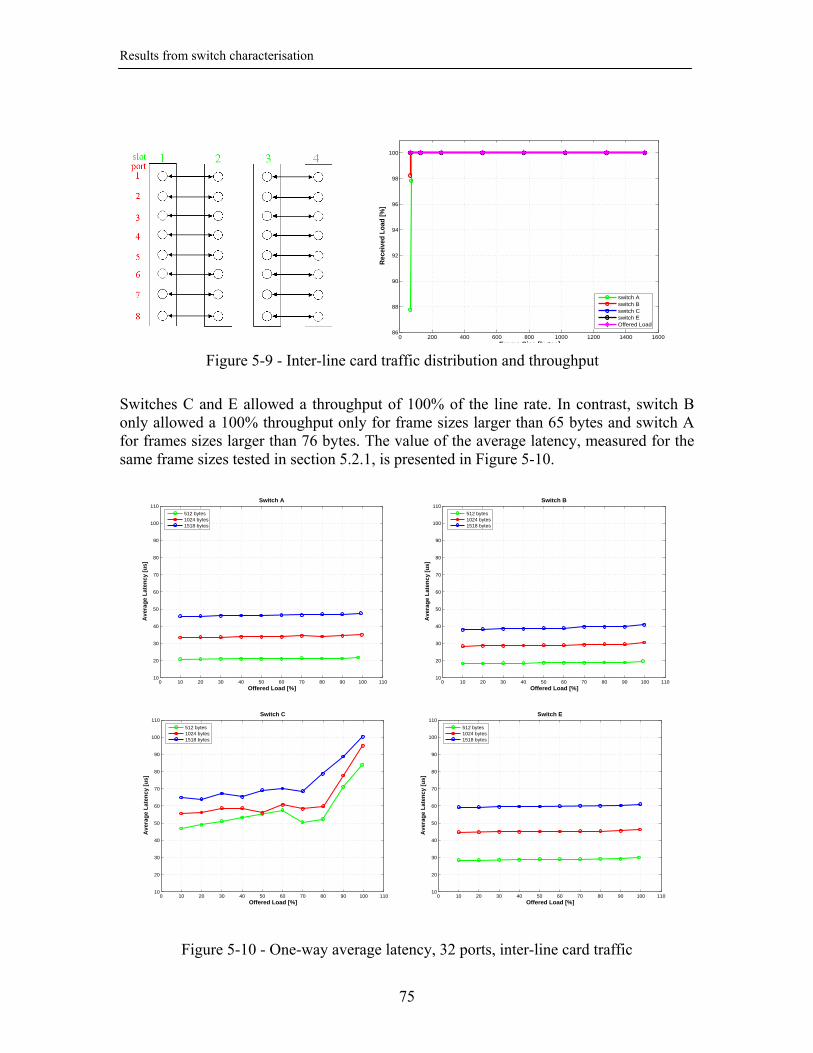
Results from switch characterisation
75
Switches C and E allowed a throughput of 100% of the line rate. In contrast, switch B only allowed a 100% throughput only for frame sizes larger than 65 bytes and switch A for frames sizes larger than 76 bytes. The value of the average latency, measured for the same frame sizes tested in section 5.2.1, is presented in Figure 5-10.
0 200 400 600 800 1000 1200 1400 160086
88
90
92
94
96
98
100
Frame Size [bytes]
Rec
eive
d Lo
ad [%
]
switch Aswitch Bswitch Cswitch EOffered Load
Figure 5-9 - Inter-line card traffic distribution and throughput
0 10 20 30 40 50 60 70 80 90 100 11010
20
30
40
50
60
70
80
90
100
110
Offered Load [%]
Ave
rag
e L
aten
cy [
us]
Switch A
512 bytes1024 bytes1518 bytes
0 10 20 30 40 50 60 70 80 90 100 11010
20
30
40
50
60
70
80
90
100
110
Offered Load [%]
Ave
rag
e L
aten
cy [
us]
Switch B
512 bytes1024 bytes1518 bytes
0 10 20 30 40 50 60 70 80 90 100 11010
20
30
40
50
60
70
80
90
100
110
Offered Load [%]
Ave
rag
e L
aten
cy [
us]
Switch C
512 bytes1024 bytes1518 bytes
0 10 20 30 40 50 60 70 80 90 100 11010
20
30
40
50
60
70
80
90
100
110
Offered Load [%]
Ave
rag
e L
aten
cy [
us]
Switch E
512 bytes1024 bytes1518 bytes
Figure 5-10 - One-way average latency, 32 ports, inter-line card traffic

Results from switch characterisation
76
Switch A, B and E had, again, a similar behaviour with respect to the latency. However, the latencies measured were consistently higher than the ones determined for the intra-line card distribution (presented in section 5.2.1). This is an indication that the inter-line card traffic had to traverse an additional layer of switching. We could thus consider that each of these three switches employed a local switching fabric to handle traffic flowing inside the same the line card and a separate switching fabric for transporting frames between the line cards. The values calculated for T_switch presented in Figure 5-11(a). Figure 5-11(b) shows a per-byte transfer time calculated taking into account T_switch and the size of the Ethernet frame. The Gigabit Ethernet transmission time is also included for comparison.
The slope of the internal latency graph for switch A is similar to the gradient of the pure Gigabit Ethernet transmission time. Interesting enough, the intra-line card results were analogous. The latency of the inter-line card communication is larger than that of the intra-line card connection by about 20%. The difference is large enough, in percentages and real values, to justify hypothesizing the existence of two layers of switching, one local to the line card and another one global to the entire chassis. In contrast, the angle presented by the results measured on switch B is much lower than the slope of the Gigabit Ethernet transmission time plot. This might indicate a relatively high scheduling time and a small transit time, due to a high speed-up factor inside the main switching fabric. The slope of the graph corresponding to switch E is higher than the one of the Gigabit Ethernet transmission. This might indicate a per-frame scheduling time that is increasing with the size of the frame. Another possible explanation would be the existence of a size-dependent overhead, additional to the transit time determined by the transmission of the Ethernet bytes of the frame over the switching fabric. Such overhead is generated by splitting the Ethernet frame onto fixed-size cells before the transfer over the switching fabric. Such scenario is common in modern switches, as detailed in chapter 3. However, only a large header/data ratio inside the cell would explain a slope of the value presented in Figure 5-11(a).
(a) Figure 5-11 - Internal switch latencies and calculated transmit time, inter-line card
(b)
0
5
10
15
20
25
30
35
40
512 1024 1518Frame size [bytes]
Inte
rnal
late
ncy
[us]
Sw itch ASw itch BSw itch EGE transmit time
00.0050.01
0.0150.02
0.0250.03
0.0350.04
0.0450.05
512 1024 1518
Frame size [bytes]
Tim
e to
tran
sfer
1 b
yte
[us]
Sw itch A
Sw itch B
Sw itch E
GE transmit time

Results from switch characterisation
77
Figure 5-12 presents a comparison of the T_switch measured on switches C and E for 512-bytes frames. As during the intra-line card tests, switch E presents latency values that are consistent throughout the entire system. On the graph characterising switch C we can observe a certain structure in the latency.
Due to the physical configuration of switch C and the limited number of ANT ports available, it was impossible to create a traffic pattern similar to the other switches. Figure 5-13 presents the actual traffic distribution, together with a view on the results for the 1518 bytes frame size. In creating this distribution of the traffic pattern, we took into consideration the fact that each group of 12 ports on the line card of switch C had an independent connection to the switching fabric. The intra-line card measurements showed that even the traffic between two ports of the same group of 12 had to traverse the switching fabric. Only 32 ports of the tester were available. The traffic pattern tried to load the switching fabric as much as possible while maintaining symmetry and fully using the ports on the first line card. The different groups of ports can be clearly identified through the structure exhibited by the latency values measured for each offered load.
05
1015
2025
3035
0
20
40
60
80
10010
12
14
16
18
20
22
Port indexOffered load [%]
T__
swit
ch [
us]
05
1015
2025
3035
0
20
40
60
80
10010
20
30
40
50
60
70
80
Port indexOffered load [%]
T__
swit
ch [
us]
Switch C Switch E
Figure 5-12 – Detailed view of T_switch, inter-line card traffic
212223 20 19 18 17 16 15 14 13 12 11 10 9 8 7 6 5 4 3 2 01
port
Four ports, intra-line card traffic - latency like port 10 on the graph
Four ports, inter-line card traffic - latency like port 8 on the graph
Figure 5-13 - Detailed traffic distribution and latency results, switch C
0 10 20 30 40 50 60 70 80 90 10045
50
55
60
65
70
75
80
85
90
95
100
Inte
rnal
late
ncy
[u
s]
Offered load [%]
port 5
port 8
port 10
All other ports - latency like port 5 on the graph
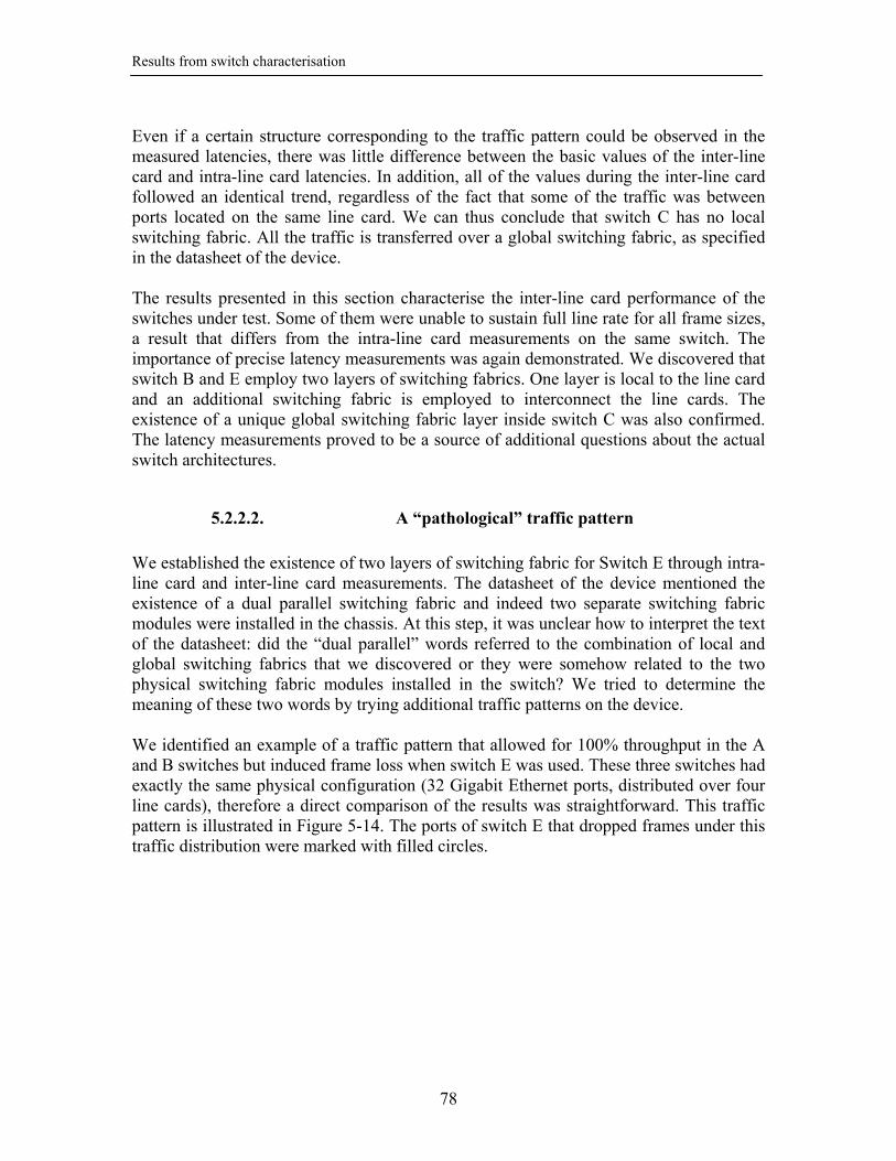
Results from switch characterisation
78
Even if a certain structure corresponding to the traffic pattern could be observed in the measured latencies, there was little difference between the basic values of the inter-line card and intra-line card latencies. In addition, all of the values during the inter-line card followed an identical trend, regardless of the fact that some of the traffic was between ports located on the same line card. We can thus conclude that switch C has no local switching fabric. All the traffic is transferred over a global switching fabric, as specified in the datasheet of the device. The results presented in this section characterise the inter-line card performance of the switches under test. Some of them were unable to sustain full line rate for all frame sizes, a result that differs from the intra-line card measurements on the same switch. The importance of precise latency measurements was again demonstrated. We discovered that switch B and E employ two layers of switching fabrics. One layer is local to the line card and an additional switching fabric is employed to interconnect the line cards. The existence of a unique global switching fabric layer inside switch C was also confirmed. The latency measurements proved to be a source of additional questions about the actual switch architectures.
5.2.2.2. A “pathological” traffic pattern We established the existence of two layers of switching fabric for Switch E through intra-line card and inter-line card measurements. The datasheet of the device mentioned the existence of a dual parallel switching fabric and indeed two separate switching fabric modules were installed in the chassis. At this step, it was unclear how to interpret the text of the datasheet: did the “dual parallel” words referred to the combination of local and global switching fabrics that we discovered or they were somehow related to the two physical switching fabric modules installed in the switch? We tried to determine the meaning of these two words by trying additional traffic patterns on the device. We identified an example of a traffic pattern that allowed for 100% throughput in the A and B switches but induced frame loss when switch E was used. These three switches had exactly the same physical configuration (32 Gigabit Ethernet ports, distributed over four line cards), therefore a direct comparison of the results was straightforward. This traffic pattern is illustrated in Figure 5-14. The ports of switch E that dropped frames under this traffic distribution were marked with filled circles.
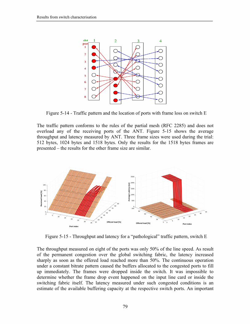
Results from switch characterisation
79
The traffic pattern conforms to the rules of the partial mesh (RFC 2285) and does not overload any of the receiving ports of the ANT. Figure 5-15 shows the average throughput and latency measured by ANT. Three frame sizes were used during the trial: 512 bytes, 1024 bytes and 1518 bytes. Only the results for the 1518 bytes frames are presented – the results for the other frame size are similar.
The throughput measured on eight of the ports was only 50% of the line speed. As result of the permanent congestion over the global switching fabric, the latency increased sharply as soon as the offered load reached more than 50%. The continuous operation under a constant bitrate pattern caused the buffers allocated to the congested ports to fill up immediately. The frames were dropped inside the switch. It was impossible to determine whether the frame drop event happened on the input line card or inside the switching fabric itself. The latency measured under such congested conditions is an estimate of the available buffering capacity at the respective switch ports. An important
05
1015
2025
3035 10
20
30
40
50
60
70
80
90
0
20
40
60
80
100
Offered load [%]
Port index
Rec
eive
d lo
ad [
%]
05
1015
2025
3035
0
20
40
60
80
1000
500
1000
1500
2000
2500
Port indexOffered load [%]
Ave
rag
e L
aten
cy [
us]
Figure 5-15 - Throughput and latency for a “pathological” traffic pattern, switch E
Figure 5-14 - Traffic pattern and the location of ports with frame loss on switch E

Results from switch characterisation
80
observation is the fact the architecture of the switch isolates the congestion. The latency or throughput of the other uncongested ports is not affected by the permanent congestion that involves 25% of the available ports. Discussions with the manufacturer revealed the fact the switch was actually using the two global switch fabric modules, each line card being connected to both modules at the same time. A command on the switch management command line interface chose the static or dynamic routing of frames over the global switching fabrics. The default setting was to use static routing, thus effectively creating the possibility of “pathological” traffic patterns (we discuss this fact in further details in the introduction of section 5.2.4). The dynamic routing, however, could not guarantee maintaining the strict order at which the frames of a certain Ethernet flow arrived at the switch. The IEEE 802.1d standard requires the in-order delivery of frames that belong to the same flow (where a flow is defined by source and destination MAC address and VLAN and priority tags). Out-of-order frames at Ethernet layer have to be handled in the higher layer protocols by the computers connected to the network. Figure 5-16 presents the result of a measurement performed after configuring a round-robin algorithm for the scheduling of the switching fabric. The traffic distribution was identical to the one presented in Figure 5-14. In this case, the trial was performed in the ANT warp mode in order to determine the maximum forwarding performance.
The dynamic scheduling of the switching fabric did not increase the total average throughput, but ensured a fairer distribution of the available bandwidth between the active ports. The throughput for small frames was higher than the value measured for large frames. The total frame loss for large frame sizes was about 10% of the line speed. The results presented in section 5.2.1.1 demonstrated that the switching fabric had enough bandwidth to accommodate 32 flows at Gigabit Ethernet line speed. The values presented in Figure 5-19 were due to overload on fixed routed paths – they are not an indication of the overall switching capacity of the fabric. We attribute the results in Figure 5-16 to an increase in the scheduling time introduced by the dynamic routing algorithm.
Figure 5-16 - Throughput switch E, dynamic scheduling, ANT warp mode
0
10
20
30
400 200 400 600 800 1000 1200 1400 1600
50
55
60
65
70
75
80
85
90
95
100
Frame size [bytes]
Rece
ived
load
[%]
Port index

Results from switch characterisation
81
Figure 5-17 presents an additional example of traffic configuration for which switch E had a throughput of 50% of the line rate, while switch B and E were measured with 100% throughput. The results of the measurements for switch E are presented in Figure 5-18.
Only the results for 1518 bytes frames are presented. The switch was configured to use the default static policy for the scheduling of the global switching fabrics. The 2-dimensional view was preferred due to the fact that the measured values were equal for all the ports of the switch. For this particular traffic distribution, all ports of switch E only allowed a throughput of 50% of the line speed. The horizontal axis of the graphs in Figure 5-18 represents the total offered load on all the ports of the switch. Also, the lost traffic is summed up for all the ports of the switch. The value of the latency presented is an average over the values measured on the 32 ports involved in the test. In conclusion, through inter-line card measurements we evidenced new architectural features on switch B and confirmed the information available on switch C. We discovered the existence of the local switching fabric on the line cards of switch E and
Figure 5-17 - Traffic configuration for 50% throughput on switch E
Figure 5-18 - Throughput and latency, switch E, 1518 bytes frames
5000 10000 15000 20000 25000 300000
2000
4000
6000
8000
10000
12000
14000
16000
Total sent traffic [Mbps]
Tota
lost
traf
fic [M
bps]
5000 10000 15000 20000 25000 30000
200
400
600
800
1000
1200
1400
1600
1800
2000
2200
Total sent traffic [Mbps]
Ave
rage
Lat
ency
[us]

Results from switch characterisation
82
exposed the effects of the static and dynamic scheduling of the global switching fabric. We continue now with measurements using random traffic, as defined in section 5.1. The random traffic generated by ANT applies a full mesh pattern, exercises both the local and the global switching fabrics at the same time. In the previous tests, only one of the fabrics was traversed during a measurement trail.
5.2.3. Fully-meshed random traffic A standard crossbar that has a FIFO policy for serving the input buffers and no speed-up would allow a maximum transfer rate of 58% for Poisson traffic (see chapter 4 and [kar-87] for details). The VOQ technique [mck-99b] coupled with an efficient scheduling algorithm has to be employed in order to obtain higher throughput, as discussed in chapter 4. By generating Poisson traffic from the ANT and comparing the measured throughput to the theoretical value we can indicate whether the architectures based on crossbars employed the VOQ technique. The fully-meshed random distribution generated both intra- and inter- line card traffic. The coordination between the local and the global switching fabric could thus be evaluated for the devices that made this architectural choice.
0 10 20 30 40 50 60 70 80 90 100 110
20
40
60
80
100
120
140
160
180
Offered Load [%]
Ave
rage
Lat
ency
[us]
Switch A
512 bytes1024 bytes1518 bytes
0 10 20 30 40 50 60 70 80 90 100 110
20
40
60
80
100
120
140
160
180
Offered Load [%]
Ave
rage
Lat
ency
[us]
Switch B
512 bytes1024 bytes1518 bytes
0 10 20 30 40 50 60 70 80 90 100 110
20
40
60
80
100
120
140
160
180
Offered Load [%]
Ave
rage
Lat
ency
[us]
Switch C
512 bytes1024 bytes1518 bytes
0 10 20 30 40 50 60 70 80 90 100 110
20
40
60
80
100
120
140
160
180
Offered Load [%]
Ave
rage
Lat
ency
[us]
Switch E
512 bytes1024 bytes1518 bytes
Figure 5-19 - One-way average latency for random traffic

Results from switch characterisation
83
The results of the measurements performed using 32 ports of the ANT are presented in Figure 5-19. The time between consecutively sent frames was determined using a negative-exponential distribution. The destination of each frame was chosen from the set of available destinations with a random uniform distribution (see section 5.1). Switch A, B and E are allegedly based on crossbar switching fabrics. They forward this particular traffic distribution, with no loss, at up to 99% of the line rate. The results presented in Figure 5-19 demonstrate that these switches make use of VOQ. With respect to switch E, as the manufacturer did not disclose the generic architecture of the switching fabric module, we can just state that the results for random traffic are a perfect match, in terms of measured latency and throughput, to those of the crossbar-based switches evaluated at the same time. At low offered loads, the latency measured on all switches is similar to that of a partial mesh using constant bitrate traffic, determined in section 5.2.2.1. The Poisson traffic distribution creates bursts of back-to-back frames at any load. The average size of a burst increases with the increase of the offered load. The random choice of destinations, performed independently by each of the traffic sources, is likely to create contention for the access to the switching fabric, as two traffic sources might send frames to the same destination at the same time. The congestion thus created is reflected in the exponential increase of latency, as presented in Figure 5-19. Figure 5-20 shows a detailed view of T_switch calculated for each of the 32 ports that participated in the trial, for one of the three measured frames sizes, for two of the switches. As presented in Figure 5-19, the behaviour for other frame sizes was similar.
The latency increase with the load was evenly distributed between the ports of the switch, with few ports suffering higher than average delays due to the uneven distribution of the traffic offered by the generator. The congestion was more severe for larger frame sizes due to the increased amount of data that had to be transferred over the switching fabric.
05
1015
2025
3035
0
20
40
60
80
10020
40
60
80
100
120
140
160
180
200
Port indexOffered load [%]
T__
swit
ch [
us]
05
1015
2025
3035
0
20
40
60
80
1000
50
100
150
200
250
Port indexOffered load [%]
T__
swit
ch [
us]
Switch B Switch C
Figure 5-20 - Detailed view of T_switch, random traffic, 1518 bytes frames

Results from switch characterisation
84
The latency values measured on switch C were almost equal for all ports and increased with the offered load, in contrast to the results for constant bitrate traffic obtained in section 5.2.1 and 5.2.2. A potential explanation would be that the switch fabric scheduler is optimised for quantities larger than one Ethernet frame. In the case of traffic bursts, most of the waiting time would be smoothed out and averaged. In the case of the constant bit rate using frames equally spaced in time, the scheduler would delay a frame for more time than when the traffic arrives in bursts. Switch B performed as expected, in accordance to the results obtained in the previous sections. We could conclude that all switches under test appeared to be optimised for handling random traffic. This type of traffic is often considered a good approximation of the traffic in real networks (as discussed in chapter 4). The influence of the particular switch architectures on the latency could be seen only at relatively low traffic loads. For an average traffic load of about 50%, the measured latencies were almost equal for all switches. The queuing effect induced by the traffic removes any latency advantage that different implementations may provide. From the architectural point of view, we provided evidence for the existence of a VOQ implementation in the switches A, B and C that were based on crossbars.
5.2.4. Results on a multi-stage architecture Switch D employed a multi-stage switching fabric architecture. This was known prior to starting the tests, together with the fact that the switching fabric defined fixed routes to interconnect the switch ports. The use of fixed routes would mean that frames addressed to several destinations will always share the same path across the fabric. In a three-stage architecture (as the Clos network presented in Figure 5-21 for example), a connection between the central switching stage and an edge switch chip may thus be overloaded without having the possibility to re-route the traffic through an under-utilised connection. It would hence be possible to encounter “pathological” traffic patterns that would only reach throughput values much lower than the maximum achievable.
Assume two ports connected to crossbars i1 and in in Figure 5-21 have to send traffic to two other ports, connected to crossbar o1. Also assume that only a unique path is
Figure 5-21 - Generic multi-stage architecture (Clos network)

Results from switch characterisation
85
statically configured between any crossbar in the i column and any other crossbar in the o column. Thus it possible that the paths from i1 and in to o1 share the same direct connection between s1 and o1. The amount of traffic passed to the destination ports in this scenario depends on the speed-up factor of the s1-o1 connection relative to the traffic sources. In case the speed-up factor equals 1, only 50% of the traffic would be sent to each of the destinations. Other scenarios are also possible in the case of statically configured routing:
• two ports located in the in crossbar share the same uplink to one of the crossbars in the s column, depending on the destination of the respective traffic
• more than two ports, located in different in crossbars, share the same connection between the s and o columns
The existence of shared internal routes in a multi-stage architecture can be determined via throughput and latency measurements. While we were aware of the higher level architecture of the multistage switching fabric implemented in switch D, the actual dimensions of the crossbars and the choice of wiring routes was unknown to us. The speed-up factor was also unknown. We will show how the value of the speed-up can be measured indirectly. If the speed-up factor of the internal connection is lower than the maximum number of concurrent paths routed over it, frame loss will appear and could be measured using a traffic generator. The measured throughput is proportional to the speedup factor and the number of routes over the spared path. A brute force approach to switch testing was taken in order to try finding some of the “pathological” patterns. Therefore, a series of 30 tests was performed, each using a different traffic distribution. A total of 30 ports of the switch were involved in each test, organized in 15 pairs. A new set of pairs was generated for each test using a uniformly distributed random number selection algorithm, thus producing a different traffic distribution. The throughput and latency values were recorded at every port, for several values of the offered load. Constant bitrate traffic was used during the trials. Figure 5-22 presents the histogram of the received rate and the one-way latency, measured for an offered load of 25% of the line speed. The value represented on the vertical axis is the number of ports where a certain value of the parameter represented on the horizontal axis (throughput or latency) was measured. The histogram was calculated for the total number of tests performed, hence the maximum number of ports was 900 (30 tests, each using 30 ports of the switch).

Results from switch characterisation
86
At an offered load of 25% switch D forwards all the incoming traffic without losses for all the traffic distributions tested. The latency varies between 40 and 59 µs, apart from one port that measures 82.5 µs. The latency measured in a separate test for an intra-module pair configuration was about 41 µs for each port. Therefore, compared with the intra-module latency, the values presented in Figure 5-22 suggest that some frames followed a path that traversed more than one stage of the multi-stage switching fabric. Congestion due to sharing internal switch connections accounts for part of the tail of the histogram. The remaining part of the tail can be explained by the number of switching stages traversed. However, using only this data, it is impossible to identify how many stages were traversed by every frame. We could do this by increasing the throughput thus increasing the congestion and potentially forcing the appearance of frame loss if the speed-up on an internal connection is matched by the congestion factor that we induce. Figure 5-23 presents a histogram of the throughput and latency values measured for an offered load of 50% of the line rate. Due to the internal architecture of the switch, the measured values of throughput and latency are radically different from those observed during previous measurements. This is the first time in this work when we present in this level of detail results from a switch that dropped frames before the offered load matched the Gigabit Ethernet line speed. This is why is important to remember that the values of the throughput presented in Figure 5-23 are still calculated relative to the line speed. They are not calculated relative to the offered load.
24.5 24.6 24.7 24.8 24.9 25 25.1 25.2 25.3 25.4 25.50
100
200
300
400
500
600
700
800
900
Throughput [% of line rate] − offered load 25%40 45 50 55 60 65 70 75 80 85
0
50
100
150
Latency [us] − offered load 25%
Figure 5-22 - Histograms of throughput and latency, switch D, offered load 25%

Results from switch characterisation
87
The measured throughput could be divided in three categories, centred on the 30%, 41% and 50% values. We used constant bitrate traffic distributed between pairs of ports. As the offered load was steady, the congestion ramped up rapidly on the oversubscribed paths over the switching fabric. Eventually, the buffers of the input ports filled up. The output ports of the switch were not oversubscribed, hence the waiting time at the destination ports was zero. Each of the three throughput categories was characterised by a particular latency value: 1900 µs, 1420 µs and 40 µs.. The correlation of latency values with the throughput demonstrate that the large latency values were determined by the different service rates of the input buffers (scheduling time). After a certain time of steady congestion, the buffers of the input ports were fully occupied and it was to be expected that the ports with the lowest service rate to experience the highest latency.
Throughput 30% 41% 50% Total pairs 8 87 805
Per trial 4 3, 6 or 9 n.r.1 Total trials 2 18 30 (all)
Table 5-2 - Distribution of throughput for an offered load of 50%, switch D
As summarised in Table 5-2, the 30% throughput was always measured for a number of ports that is a multiple of four, while the 41% throughput was measured for a number of ports that is a multiple of three. This observation (confirmed by subsequent tests at higher offered loads), lead us to believe that a speed-up factor of about 1.2 was available on the connections over the switching fabric, compared to the input and output ports of the switch. Figure 5-24 presents the throughput and latency histograms for an offered load of 100% of the line speed.
1 Not relevant for the interpretation
30 35 40 45 50 550
100
200
300
400
500
600
700
800
900
Throughput [% of line rate] − offered load 50%0 200 400 600 800 1000 1200 1400 1600 1800 2000
0
100
200
300
400
500
600
700
800
900
Latency [us] − offered load 50%
Figure 5-23 - Histogram of throughput and latency, switch D, offered load 50%

Results from switch characterisation
88
Throughput 30% 40% 60% 80% 100% Total pairs 0.9% 9.67% 43% 1.1% 45% Per trial 4 3 2 2, 1 n.r.2
Table 5-3 - Distribution of throughout for an offered load of 100%, switch D
Table 5-3 summarises the values of throughput that were measured during the trials with an offered load of 100% of the line speed. The 100% throughput value corresponds to direct intra-line card connections, fact confirmed by the value of the 41 µs bin in the histogram latency. Again, the 40% and 30% values of the throughput appeared in groups of three and four ports, exactly for the same ports and in the same ratio relative to the total number of port combinations as for the test presented in Figure 5-23. The throughput value of 60% confirmed the hypothesis of the 1.2 speedup factor of the switching fabric. This value of the throughput was the result of two Gigabit Ethernet connections sharing the same path over the switching fabric. Due to the speed-up factor, only 60% of the Gigabit Ethernet line rate offered load could be transferred over the switching fabric. The value of 80% received throughput was certainly due to the connections between the s and o layers of crossbars (Figure 5-21). This value was measured for two ports during the one trial and one port in eight other trials (out of a total of 30 trials). During each one of these tests, multiple ports were measured with a 40% throughput. Thus, the 80% throughput is the result of the shared usage of a connection between the s-o layers that is also carrying a flow reduced at 40% of the Gigabit Ethernet bandwidth over a connection between the i-s layers. However, it is unclear what mechanism was used for determining the share of the bandwidth occupied by each one of the flows.
2 Not relevant for the interpretation
20 30 40 50 60 70 80 90 1000
50
100
150
200
250
300
350
400
450
Throughput [% of line rate] − offered load 99%0 500 1000 1500 2000 2500
0
50
100
150
200
250
300
350
400
450
Latency [us] − offered load 99%
Figure 5-24 - Histogram of throughput and latency, 100% offered load

Results from switch characterisation
89
In the case of the flows occupying 30%, 40% or 60% of the Gigabit Ethernet bandwidth, a round-robin mechanism for the bandwidth allocation may explain the results. A connection over the switching fabric is oversubscribed by N flows (where N=4, 3, 2) and the available bandwidth is divided fairly between the incoming flows. However, in the case of the 80% measured throughput, a connection over the switching fabric was oversubscribed by a flow that was reduced to 40% of the Gigabit Ethernet bandwidth and another flow that used 100% of the Gigabit Ethernet bandwidth. This connection could accommodate up to 120% of the Gigabit Ethernet bandwidth, therefore some of the incoming traffic had to be dropped. A solid explanation why all the traffic was dropped from the second flow, even when the flows had the same priority, could be provided only by including additional knowledge about the internal architecture of the crossbars. In conclusion, by using a brute force tactic and some information about the internal architecture of switch D we were able to determine the speed-up factor of the interconnections between the crossbars of the multistage switching fabric. As with switch E, the performance level we measured on switch D was dependent on the particular traffic pattern. In case the switch is purchased to be used for a particular application, it is important to evaluate whether the traffic generated by this application falls within one of the “pathological” patterns.
5.2.5. Summary Through measurements of throughput and latency we were able to find additional information about the architectures of the switches under test. Table 5-4 summarises our findings. Results from characterising the quality of service implementation in the same switches were obtained by Beuran and reported in [beu-04].
switch GE
ports Local switching on the line
card Buffers Switch fabric architecture
A 8
Yes
Latency dependent on frame size Input-output Crossbar, VOQ
B 8
Yes, shared memory
4µs latency Input-output Crossbar, VOQ
C 24 No - confirmed Input-output Crossbar, VOQ
D 8
Some – confirmed
16µs latency Input-output
Multi-stage; static routing
Speed-up factor 1.2
E 8
Yes, shared memory
3µs latency Input-output
Dual parallel fabrics, static and dynamic routing
throughput as low as 50%
Table 5-4 - Main results of the measurements using unicast traffic

Results from switch characterisation
90
5.3. Broadcast traffic RFC 2285 mentioned the determination of the forwarding rate of broadcast frames and the associated latency as mandatory measurements for switch characterisation. Our approach is, again, to try to discover the mechanism that implements the broadcast instead of providing a list of performance-related numbers. Only the results of the investigation on switches A, B, C and E are presented. Very low (compared to the other switches) broadcast rates were measured on switch D. Discussions with the manufacturer revealed that the switch used a software implementation on the management CPU for replicating broadcast frames, as well as plans to migrate to a hardware-based implementation in the next generation of the device. Therefore it would be irrelevant to present results from measurements on an outdated solution. We will apply the same methodology that we used for the trials using unicast traffic. We measure throughput and latency and speculate on the architecture based on the results of the measurements. In addition, following the real temporal succession of the tests, we consider that the architectural features evidenced for unicast traffic are known.
5.3.1. Intra-line card broadcast traffic All the ports on one line card were connected to ANT traffic generators. Three separate sets of trials were made. Each set of trials employed a number of 1, 4 or 8 sources while the remaining ports of the line card received the broadcast traffic. As indicated in section 5.1.2, when multiple sources were active at the same time, each one of them received the broadcast generated by the other sources. We start by presenting the results of the measurements using one broadcast source. They provide an evaluation of the bottom line performance to be expected during the rest of the tests. We continue by discussing the results of the trials done using four sources of broadcast. We do not present the results of the measurements using 8 sources as they will not provide new information about the implementation of broadcast support inside the switch.
5.3.1.1. One broadcast source The normalized receive load (defined in section 5.1.2) measured for traffic produced by one broadcast source and received by tester ports connected to all the other ports of the same line card is presented in Figure 5-25.

Results from switch characterisation
91
Switch A forwarded only a limited amount of frames out of the offered load. This limitation can be observed better in Figure 5-26, where the horizontal axis represents the offered load expressed in frames per second instead of the percentage of the line speed measure used in Figure 5-15. For all three frame sizes, the normalised received load plot presents an inflexion point at approximately the same value, situated around 43000 frames per second. The frame rate limitation might be caused by a per-frame processing overhead that is independent of the frame size.
0 10 20 30 40 50 60 70 80 90 100 11070
75
80
85
90
95
100
Total Offered Load [% of line rate]
Nor
mal
ized
Rec
eive
Loa
d [%
]Switch A
512 bytes1024 bytes1518 bytes
0 10 20 30 40 50 60 70 80 90 100 11070
75
80
85
90
95
100
Total Offered Load [% of line rate]
Nor
mal
ized
Rec
eive
Loa
d [%
]
Switch C
512 bytes1024 bytes1518 bytes
0 10 20 30 40 50 60 70 80 90 100 11070
75
80
85
90
95
100
Total Offered Load [% of line rate]
Nor
mal
ized
Rec
eive
Loa
d [%
]
Switch E
512 bytes1024 bytes1518 bytes
0 10 20 30 40 50 60 70 80 90 100 11070
75
80
85
90
95
100
Total Offered Load [% of line rate]
Nor
mal
ized
Rec
eive
Loa
d [%
]
Switch B
512 bytes1024 bytes1518 bytes
Figure 5-25 - Throughput for one source of broadcast traffic
0 1 2 3 4 5 6
x 104
70
75
80
85
90
95
100
Offered Load [frames/s]
Nor
mal
ized
Rec
eive
Loa
d [%
]
Switch A
512 bytes1024 bytes1518 bytes
Figure 5-26 - Throughput limitation for broadcast traffic

Results from switch characterisation
92
Switch B also presented a limitation in the throughput, but only for the smallest of the frame sizes under test. The maximum throughput for this frame size was about 124000 frames per second, a value 288% higher compared to switch A. Switch E and switch C were capable of supporting a throughput of 100% of the line rate for the three frame sizes used in this test. Further investigations were carried on these two switches using the set of frame sizes specified in RFC 2544. The ANT warp mode that allowed generating 100% of the line speed for all frame sizes was used and the results are presented in Figure 5-27.
Switch E was able to forward broadcast frames at the nominal line rate, for all frame sizes. The shared memory architecture of the local switching fabric on the line card (determined by the measurements in section 5.2.1) is well adapted to the implementation of broadcast traffic. The actual broadcast frame would be stored in memory once, upon arrival at the input port. Only simple pointer processing would be required in order to perform the frame replication, with no actual copying of the frame to a newer location. Switch C showed a limitation in terms of accepted frame rate for frames smaller than 512 bytes. As the two consecutive points for measurement correspond to 256 and 512 bytes frames, it is impossible to determine exactly the minimum frame size that allowed 100% throughput. We could also draw the attention to the fact that switch C had 24 ports on the same line card, therefore the total broadcast traffic rate (expressed in frames per second) within this test was much higher than the one measured on switch E, which only had 8 ports per line card. Figure 5-28 presents the results of the latency measurements for the scenario of using one source of broadcast traffic and intra-line card traffic distribution. The different implementations were characterised by different average latency values measured.
0 200 400 600 800 1000 1200 1400 16000
10
20
30
40
50
60
70
80
90
100
110
Frame Size [bytes]
Rec
eive
d Lo
ad [%
]
switch Cswitch EOffered Load
Figure 5-27 - Broadcast throughput, one source

Results from switch characterisation
93
At 10% offered load, the latency measured on switch A presents a 300% increase compared to the unicast traffic measured in section 5.2.1. The latency had perfectly equal values for all the receivers of the traffic (details presented in Figure 5-29). From the unicast tests it was known that the switch did no use a shared memory fabric. The other possible explanation for the equal values of the latency would be the implementation of a shared bus, independent of the regular switching fabric and reserved for the broadcast traffic. To push the speculation further, the switch management CPU might also be connected to this bus. In this case, the limitation in frame rate would be explained by the processing capability of the CPU. The maximum values measured for the latency, in excess of 6.2 ms, were much higher than those measured (in the range of 320 µs [mei-02n]) during induced congestion using unicast traffic. Therefore additional buffers must have been made available for the broadcast traffic when compared to the unicast traffic. Considering the minimum broadcast latency of about 75.5 µs as the lower limit of the service time, the maximum queue length would be about 82 frames compared to about 7 frames for unicast traffic. The lowest latency measured on switch B presented a 230% increase with respect to that of the unicast traffic measure din section 5.2.1. A broadcast implementation similar to that of switch A can be hypothesised due to the limitation observed in terms of frame rate and the similarity in terms of the highest average latency value recorded.
05
1015
2025
0
20
40
60
80
10012
14
16
18
20
22
24
26
28
30
Frame size / port indexOffered load [%]
Ave
rage
Lat
ency
[us]
010
2030
4050
6070
0
20
40
60
80
10040
45
50
55
60
65
70
75
80
Frame size / port indexOffered load [%]
Ave
rage
Lat
ency
[us]
05
1015
2025
0
20
40
60
80
1000
500
1000
1500
2000
2500
Frame size / port indexOffered load [%]
Ave
rage
Lat
ency
[us]
05
1015
2025
0
10
20
30
40
50
600
1000
2000
3000
4000
5000
6000
7000
Frame size / port indexOffered load [%]
Ave
rage
Lat
ency
[us]
Switch A Switch B
Switch C Switch E
Figure 5-28 – One way latency for broadcast traffic, 1 sender, intra-line card

Results from switch characterisation
94
The average latency measured for switch C was similar to the value measured for unicast traffic in section 5.2.1. This lead us to believe that the broadcast traffic follows the same path as the unicast traffic, traversing the switching fabric. The measured latency was equal for all the ports (Figure 5-29). The equal values of the latency meant that the switching fabric performed the replication of the broadcast frames and sent the resulting frames, in parallel, to all the destination ports.
The average latency measured for switch E was similar to the values measured for intra-line card unicast traffic in section 5.2.1. These results confirm our hypothesis that the shared memory fabric existent on the line cards implements both unicast and broadcast traffic support.
5.3.1.2. Four broadcast sources Figure 5-30 presents the results of the throughput measurements when four broadcast sources were located on the same line card. Each of the sources received the broadcast from the other three transmitters. The other ports on the line card received traffic from all the sources.
0
2
4
6
8
0
20
40
60
8012
12.5
13
13.5
14
14.5
15
15.5
16
Port indexOffered load [%]
Ave
rage
Lat
ency
[us]
05
1015
2025
0
20
40
60
80
10040
45
50
55
60
Port indexOffered load [%]
Ave
rage
Lat
ency
[us]
0
2
4
6
8
0
20
40
60
80
10040
50
60
70
80
90
100
110
120
130
Port indexOffered load [%]A
vera
ge L
aten
cy [u
s]0
2
4
6
8
0
10
20
30
40
50
600
20
40
60
80
100
Port indexOffered load [%]
Ave
rage
Lat
ency
[us]
Switch A Switch B
Switch C Switch E
Figure 5-29 - Latency of 1518 bytes frames, one broadcast source, intra-line card traffic
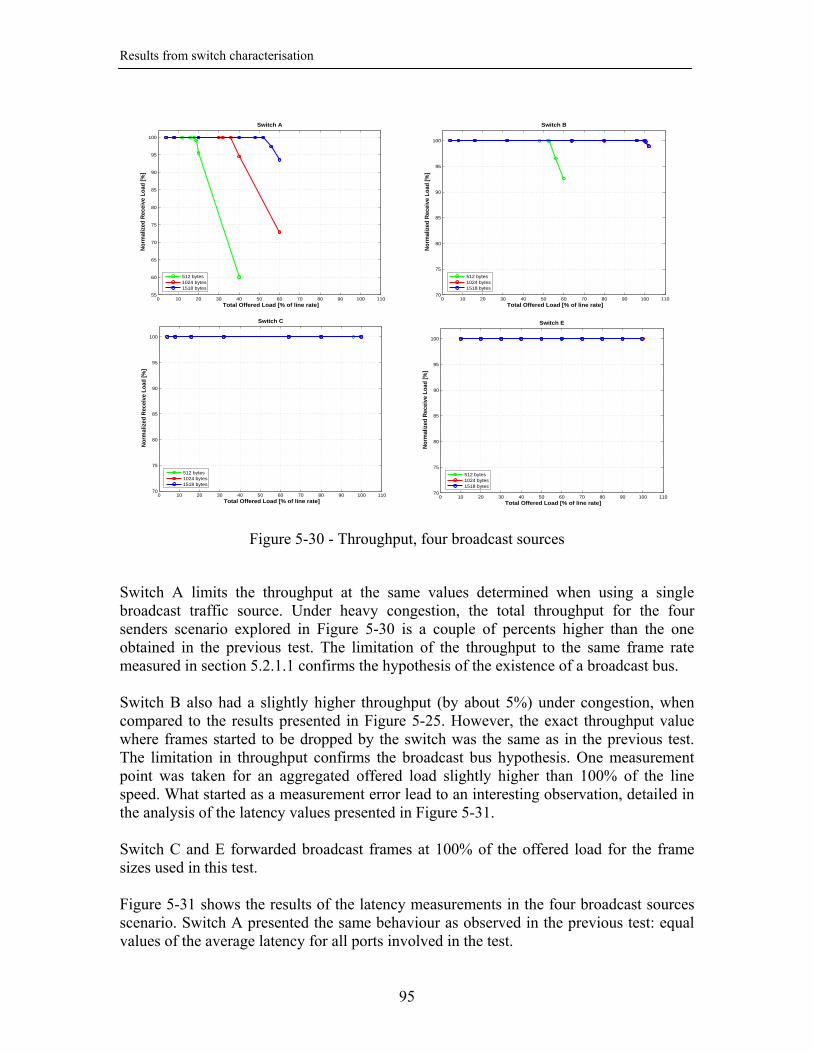
Results from switch characterisation
95
Switch A limits the throughput at the same values determined when using a single broadcast traffic source. Under heavy congestion, the total throughput for the four senders scenario explored in Figure 5-30 is a couple of percents higher than the one obtained in the previous test. The limitation of the throughput to the same frame rate measured in section 5.2.1.1 confirms the hypothesis of the existence of a broadcast bus. Switch B also had a slightly higher throughput (by about 5%) under congestion, when compared to the results presented in Figure 5-25. However, the exact throughput value where frames started to be dropped by the switch was the same as in the previous test. The limitation in throughput confirms the broadcast bus hypothesis. One measurement point was taken for an aggregated offered load slightly higher than 100% of the line speed. What started as a measurement error lead to an interesting observation, detailed in the analysis of the latency values presented in Figure 5-31. Switch C and E forwarded broadcast frames at 100% of the offered load for the frame sizes used in this test. Figure 5-31 shows the results of the latency measurements in the four broadcast sources scenario. Switch A presented the same behaviour as observed in the previous test: equal values of the average latency for all ports involved in the test.
0 10 20 30 40 50 60 70 80 90 100 11055
60
65
70
75
80
85
90
95
100
Total Offered Load [% of line rate]
Nor
mal
ized
Rec
eive
Loa
d [%
]
Switch A
512 bytes1024 bytes1518 bytes
0 10 20 30 40 50 60 70 80 90 100 11070
75
80
85
90
95
100
Total Offered Load [% of line rate]
Nor
mal
ized
Rec
eive
Loa
d [%
]
Switch B
512 bytes1024 bytes1518 bytes
0 10 20 30 40 50 60 70 80 90 100 11070
75
80
85
90
95
100
Total Offered Load [% of line rate]
Nor
mal
ized
Rec
eive
Loa
d [%
]
Switch C
512 bytes1024 bytes1518 bytes
0 10 20 30 40 50 60 70 80 90 100 11070
75
80
85
90
95
100
Total Offered Load [% of line rate]
Nor
mal
ized
Rec
eive
Loa
d [%
]
Switch E
512 bytes1024 bytes1518 bytes
Figure 5-30 - Throughput, four broadcast sources
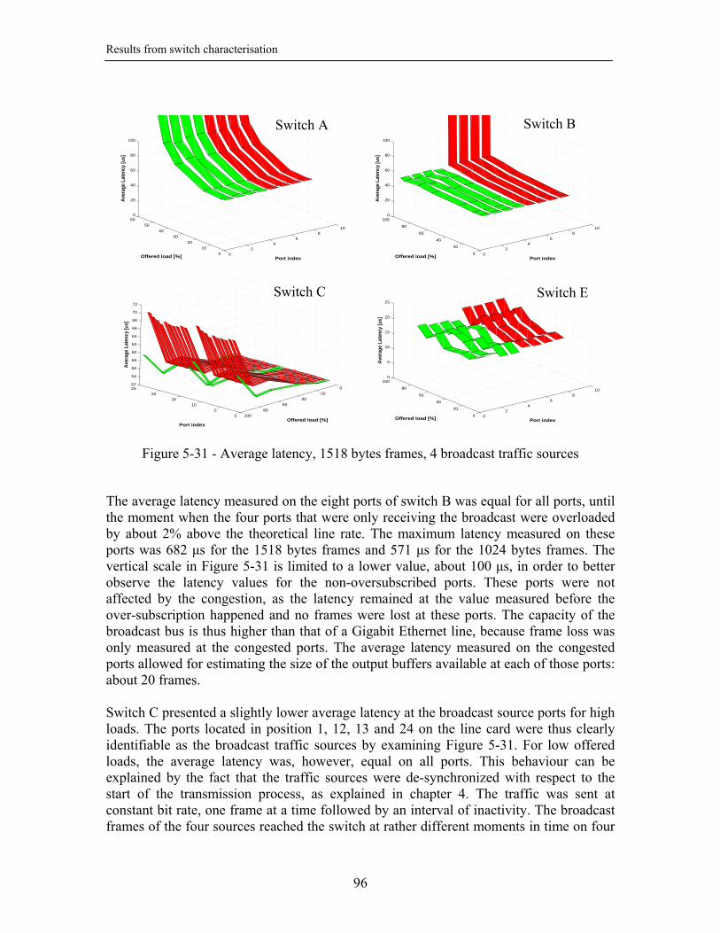
Results from switch characterisation
96
The average latency measured on the eight ports of switch B was equal for all ports, until the moment when the four ports that were only receiving the broadcast were overloaded by about 2% above the theoretical line rate. The maximum latency measured on these ports was 682 µs for the 1518 bytes frames and 571 µs for the 1024 bytes frames. The vertical scale in Figure 5-31 is limited to a lower value, about 100 µs, in order to better observe the latency values for the non-oversubscribed ports. These ports were not affected by the congestion, as the latency remained at the value measured before the over-subscription happened and no frames were lost at these ports. The capacity of the broadcast bus is thus higher than that of a Gigabit Ethernet line, because frame loss was only measured at the congested ports. The average latency measured on the congested ports allowed for estimating the size of the output buffers available at each of those ports: about 20 frames. Switch C presented a slightly lower average latency at the broadcast source ports for high loads. The ports located in position 1, 12, 13 and 24 on the line card were thus clearly identifiable as the broadcast traffic sources by examining Figure 5-31. For low offered loads, the average latency was, however, equal on all ports. This behaviour can be explained by the fact that the traffic sources were de-synchronized with respect to the start of the transmission process, as explained in chapter 4. The traffic was sent at constant bit rate, one frame at a time followed by an interval of inactivity. The broadcast frames of the four sources reached the switch at rather different moments in time on four
02
46
810
0
20
40
60
80
1000
5
10
15
20
25
Port indexOffered load [%]
Ave
rage
Lat
ency
[us]
05
1015
2025 0
2040
6080
100
52
54
56
58
60
62
64
66
68
70
72
Offered load [%]Port index
Ave
rage
Lat
ency
[us]
02
46
810
0
20
40
60
80
1000
20
40
60
80
100
Port indexOffered load [%]
Ave
rage
Lat
ency
[us]
02
46
810
0
10
20
30
40
50
600
20
40
60
80
100
Port indexOffered load [%]
Ave
rage
Lat
ency
[us]
Switch A Switch B
Switch C Switch E
Figure 5-31 - Average latency, 1518 bytes frames, 4 broadcast traffic sources

Results from switch characterisation
97
separate connections, as long as the offered load was low. Thus the switching fabric performed similar to the unique broadcast source scenario, with the same result: equal latency measured on all ports. As the generated traffic increased in throughput and the transmit times became synchronised, more frames arrived at the switching fabric at the same time. Therefore, even if the fabric was capable of replicating frames faster than the Gigabit Ethernet transmission speed, frames would have to queue in the output buffers of the switch ports. The shorter queues in the buffers of the broadcast source ports were responsible for the slightly smaller values of the average latency. The latency measured on switch E at high loads was about 10% to 18% higher for the ports that were only receivers of the broadcast. The same mechanism of partial overlap of the offered broadcast frames, coupled with the increased load on the ports that only received the traffic, is responsible for the increase in latency. As expected, the broadcast implementations in the four switches under test were rather different. Table 5-5 summarises our findings. switch Ethernet broadcast support architecture A Bus B Bus C Crossbar of the main switching fabric E Shared memory
Table 5-5 - Summary of broadcast support architectures in switches under test
It was particularly interesting to see how some of these devices used a separate fabric for the transmission of the broadcast frames, compared to standard unicast. The next step was to investigate the behaviour in the case when broadcast traffic was sent between ports located in different line cards of the switch.
5.3.2. Inter-line card broadcast traffic
5.3.2.1. Four traffic sources A first measurement for determining the inter-line card performance of the broadcast traffic support was performed using four traffic sources, each of them located on a different line card. The traffic was received by the other 28 ports of the tester, connected to the remaining ports of the switch. Figure 5-32 presents the results of the throughput and latency measurements for switch A under this traffic distribution.

Results from switch characterisation
98
The broadcast implementation of the switch showed exactly the same limitation, in terms of forwarded frame rate, as observed during the intra-line card measurements. The average latency for low traffic loads was only 10% higher than the one measured for the intra-module traffic. The hypothesis of a broadcast bus that interconnects all the ports of the switch was thus confirmed again. The throughput measured on switch B and E in this scenario was, again, 100% of the line rate – apart from the case of 512-bytes frames for switch B. However, similar throughput plots were already presented in this chapter so we considered that these graphs would present little interest. The results of the latency measurements were different from those observed before, so they are presented in Figure 5-33.
Apart from the somewhat lower latency measured on the broadcast source ports and explained in section 5.2.1, switch B presented a consistent pattern of lower latencies on a certain line card. Within this line card, three of the ports, physically close to the broadcast source port, were measured with a lower latency than the other four ports located on the same line card. These four ports, in turn, presented lower latencies than the other ports of
0 10 20 30 40 50 60 70 80 90 100 11082
84
86
88
90
92
94
96
98
100
102
Total Offered Load [% of line rate]
Nor
mal
ized
Rec
eive
Loa
d [%
]
Switch A
512 bytes1024 bytes1518 bytes
05
1015
2025
3035
35
40
45
50
55
600
50
100
150
200
250
300
350
400
Port indexOffered load [%]
Ave
rage
Lat
ency
[us]
Figure 5-32 – Aggregated throughput and detailed view of the latency for switch A
0 5 10 15 20 25 30 35 0
20
40
60
80
100
0
5
10
15
20
25
30
35
40
45
50
55
Offered load [%]
Port index
Ave
rage
Lat
ency
[us]
0 5 10 15 20 25 30 350
50100
30
35
40
45
50
55
60
65
Port index
Ave
rage
Lat
ency
[us]
Offered load [%]
Switch B Switch E
Figure 5-33 - Average latency measurements, 4 broadcast sources

Results from switch characterisation
99
the switch. No reasonable explanation could be given for this behaviour, neither by the author nor by the manufacturer of the device. However, this behaviour was consistent during the broadcast tests that involved all four line card of the switch, for all the tested frames sizes and was independent on the number of broadcast sources. Switch E shown a different behaviour the other three switches: the latencies measured for the broadcast source ports were higher than those measured for the ordinary receivers. Combined with the existing evidence about the local shared memory switching fabric of each line card, this observation lead us to believe that the replication of the broadcast frames took place in two stages. One stage was local to the line card and involved the shared memory fabric, as determined in section 5.2.1. However, in case receivers were located on multiple line cards, a single copy of a broadcast frame was transmitted over the main switching fabric to each of the line cards. The second stage of the broadcast replication would thus take place on the line card that received the frame, but involved the transmission of a number of frames over the main switching fabric. The larger latency measured on the broadcast sources can be explained as follows. The ports that were only receivers of the broadcast would receive frames that were immediately replicated on the line card (25%of the total number of received frames) and also frames that traversed the fabric before being replicated locally (75% of the total number of received frames). The sources of broadcast traffic would only receive frames that traversed the main switching fabric, having a larger latency than the frames replicated locally. See sections 5.2.1 and 5.2.2 for the respective latency values of unicast traffic and section 5.2.1 for the proof that the latency of intra-line card broadcast traffic is equal to that of the intra-line card unicast traffic.
5.3.2.2. Eight traffic sources An experiment involving eight sources of broadcast traffic, located on the same line card (thus using all the available ports), and 24 receiver ports located on the remaining line cards was performed on switches A, B and E. It made little sense to perform this experiment on switch C that could accommodate 24 ports on the same line card. The measurements for throughput were in accordance to the previous tests, in terms of limited forwarded frame rates for switch A and B and support of 100% throughout for switch E. Therefore the corresponding graphs are not presented. The results of latency measurements on switch A are not presented on the same grounds. A detailed view of the latencies measured for switch B and E is presented in Figure 5-34.

Results from switch characterisation
100
The sources of broadcast traffic are indicated with green arrows on the plot for switch B. As expected from the results of previous tests, these ports were affected by the frame rate limitation of the broadcast implementation at the same time as all the other ports, as shown by the sharp increase in latency for 512-bytes frames. However, they were unaffected by the increase in latency caused by the overload of the receiver’s bandwidth for the 1024-bytes frames. The ports located on one particular line card of the switch (marked with a magenta arrow on the figure) presented smaller latencies than the other ports, as discussed in section 5.2.2.1. The results measured on switch E confirmed the hypothesis of a two-stage implementation of the broadcast support and also brought new information. It was expected that the first eight ports, sources of broadcast traffic located on the same line card, would present a lower latency than the other ports due to the local replication of the received broadcast frames. The fact that all the other 24 ports of the switch had equal average latency values suggested that the replication of broadcast frames to be transmitted to the other line cards was performed inside the main switching fabric rather than on the originating line card. If the second stage of the broadcast replication would have been implemented sequentially on the line card that originated the traffic, each group of eight ports on a destination line card would have presented a different value of the average latency. The difference between the values measured on two line cards would have been equal to the time required for a broadcast frame to traverse the main switching fabric.
5.3.2.3. Maximum broadcast configuration – 32 sources The results performed using the maximum tester configuration, 32 ports, acting as broadcast traffic sources and receivers at the same time. We only mention these trials, without presenting the graphs. The results only confirmed the information gathered through the previous experiments, for all the four switches. We observed the same limit of a maximum of 430000 frames per second forwarded by switch A. Switch B only
05
1015
2025
3035
0
20
40
60
80
10010
20
30
40
50
60
70
Port indexOffered load [%]
Ave
rage
Lat
ency
[us]
05
1015
2025
3035
0
20
40
60
8030
35
40
45
50
55
60
65
70
Port indexOffered load [%]
Ave
rage
Lat
ency
[us]
Switch B Switch E
Figure 5-34 – Latency for broadcast traffic, 8 sources on the same line card

Results from switch characterisation
101
shows a limitation for limited for smaller frame sizes. One particular line card exhibited a particular structure in the measured latency values that we could not explain. In case of overload, all 32 ports of switch B dropped traffic in equal parts from all sources and presented the same maximum average latency. Switch C and E supported broadcast traffic at line rate for the frame sizes used in the test. The average latency values were equal for all ports on the respective switches.
5.3.3. Summary We examined in detail the implementation of broadcast traffic support in four modern Ethernet switch architectures. Our findings are presented in Table 5-6.
switch Ethernet broadcast support architecture A Bus; limited at about 43000 frames/s B Bus; limited at about 120000 frames/s C Main switching fabric;
Frame replication implemented in the fabric E Intra-line card: shared memory
Inter-line card: inside the main switching fabric
Table 5-6 - Summary of broadcast support implementations
We also encountered unexpected results in the case of switch B. Discussions with the manufacturer did not shed more light on this issue.
5.4. Conclusion This chapter demonstrated how simple measurements of throughput and latency can be used to investigate the internal structure of Ethernet switches. Starting from the generic set of measurements for throughput and latency defined in RFC 2285 and RFC 2544, originally aimed at determining the raw performance of the device, a set of particular measurements was designed and applied on real Ethernet switches. Each section of this chapter showed how the raw values of the throughput and the value of the average latency between pairs of traffic flows can be interpreted in a way that would reveal information about the internal architecture of the switch. The detailed look on how different switch manufacturers implement Ethernet broadcast traffic is unique in the literature. The results measured on real switches show the importance of developing a highly accurate traffic generator, as the one described in chapter 4 and used throughout these tests. The offered load for the broadcast traffic had to be adjusted in quantities of 0.1% of the Gigabit Ethernet line rate in order to determine the exact frame rate for which the broadcast limitation appeared in switch A. The less-than-microsecond accuracy in the

Results from switch characterisation
102
measurement of latency on a per-frame basis allowed the coherent explanation of the broadcast mechanism in switch E and the calculation of internal transfer rates on all the four switches under test. It also allowed the detailed investigation of the internal transit times of the multi-stage architecture employed by switch D. The motivation for performing these measurements was extracting parameters for the modelling of Ethernet switches in the context of the ATLAS TDAQ system. The highest accuracy in the determination of these parameters would assure that a relatively simple parameterised model of an Ethernet switch would be able to provide a reasonable degree of confidence during the simulation of the full-scale TDAQ system. The possibility of determining the raw performance of a particular switch would allow the selection of the devices that would best fit the requirements of the TDAQ system. We also showed that some switches may encounter what we called “pathological” traffic patterns. Such traffic flows could only be predicted by having an in-depth knowledge of the architecture of the switch. Only few manufacturers would disclose such detailed information. Therefore, the measurements on the real device are the only way to ensure that the TDAQ traffic pattern will not fall into the “pathological” flow of a particular switch. Chapter 7 will present further conclusions relevant for the ATLAS experiment. Chapter 6 presents innovative contributions in the use of native Ethernet technology over long-distance networks.

10 GE WAN PHY Long-Haul Experiments
103
6. 10 GE WAN PHY Long-Haul Experiments In the context of evaluating the use of remote computing capacities for ATLAS, the WAN PHY is a technology of interest due to the distances that could potentially be covered (transeuropean or transatlantic). The WAN PHY has a lower data rate available to the user (9.28 Gbit/s) in comparison to the LAN PHY (10 Gbit/s). The way this limitation would impact traffic on a LAN distributed over continents required further study. The very fact that WAN PHY would be able to directly interconnect with long-distance networks in the absence of an ELTE had to be verified. Only one prior experiment was performed in this area [hub-02] but the distance was relatively small and no deployments in the field followed the end of the experiment. No information was given with respect of the solution chosen for the clock synchronization of the equipment used in these experiments. No conclusion could be taken with regard to the inter-operation with fully compliant SONET/SDH equipment. We applied to the 10 GE measurements the same method that we developed together with our colleagues for the characterisation of 1 Gbit/s long distance connections [kor-04]. First, traffic generators were used for determining the basic level of performance of the connection or circuit. These trials consisted in running traffic continuously, in both directions of the circuit, at an offered load as close to the line speed as the equipment allowed us to generate. The traffic consisted in Layer 2 frames with randomised data as payload. We had exclusive use of the circuits; hence there was no contention with traffic produced of other users. The frames lost in this simple configuration could thus be considered as an inherent generic characteristic of a particular circuit. The use of the traffic generators would thus allow determining basic statistical parameters associated to the circuit. These parameters could compensate for a sophisticated monitoring infrastructure that was not accessible over the course of the long-distance connection. For example, a certain frame loss pattern observed during these measurements could be correlated with losses measured using higher layer traffic generated by PCs. The second step of our long-distance measurements method consisted in the use of standard PCs and traffic generators implemented in software. The reason for using an additional step was to determine in what way the long-distance would affect real data transfers. Usually, the transfer protocol was TCP. The standard TCP protocol’s implementation would suffer a severe reduction in throughput when even a single frame would be lost over a high-latency connection [flo-02]. Therefore it would be of particular relevance to be able to clearly identify such loss as due to the network or to the poor performance of the end nodes.
6.1. Proof of concept in the laboratory An OC-192/STM-64 module in SONET/SDH-compliant devices provides the closest functionality to that of an ELTE. However, no manufacturer took the necessary steps to qualify their OC-192/STM-64 modules with respect to the ELTE requirements. The

10 GE WAN PHY Long-Haul Experiments
104
collaboration with the research network operators CANARIE and SURFnet, who at the time managed an infrastructure based on Cisco ONS 15454 devices, made the Cisco equipment the obvious target of the experiments. Only one switch manufacturer (Force10 Networks) had a WAN PHY module available on the market, so there was no possibility of a choice here either. The smallest version of the Force10 switches, the E600 chassis, was used during these experiments. The experiments presented in this section took place in July 2003 at CANARIE’s research laboratory in Ottawa, Canada. A set of basic measurements were performed on the Force10 switches prior to connecting the WAN PHY ports to the OC-192 in the long-distance networking equipment. These measurements were necessary in order to establish a baseline for the expectations in the follow-up tests. The configuration under test is presented in Figure 6-1.
Measurements performed by Hurwitz et al. [hur-03] using server PCs showed that a maximum transfer rate of about 5 Gbit/s would be achievable using a PC equipped with 10 GE network adaptors. We therefore had no choice but to use commercial traffic generators in order to completely utilize the bandwidth available on the network. Traffic generators manufactured by Ixia were available, on loan from the manufacturer, during the interval of the experiments. The Ixia chassis was equipped with two 10 GE LAN PHY interfaces and four Gigabit Ethernet interfaces. Only one of the switch-to-switch connections showed in Figure 6-1 was active during a measurement trial. The switches were configured to accept jumbo frames up to 9252 bytes. Though still unsupported by the IEEE 802.3 standard, it was demonstrated that jumbo frames could provide substantial performance increases for server applications [hur-03]. The connections between the two switches were activated and characterized one at a time. The test to determine the maximum throughput according to RFC1944 was run in each network configuration. When the interconnection was realized through the LAN PHY ports, the traffic generators measured a throughput equal to 100% of the line rate for bidirectional simultaneous traffic. The average latency measured under these circumstances is presented in Figure 6-2. The traffic was sent simultaneously in both directions.
E 600 E 600
10GBASE-LWIXIA
1
2
10GBASE-LR10GBASE-LR
Figure 6-1 - Network configuration for the baseline WAN PHY measurements

10 GE WAN PHY Long-Haul Experiments
105
The WAN PHY defined a transmission rate of 9.95 Gbaud/s, but the payload capacity is only 9.28 Gbit/s due to part of the SONET/SDH frame being reserved for management and monitoring purposes and also due to the 64B/66B encoding of the signal. Compared to the 10.31 Gbaud/s transmission rate of the LAN PHY, the WAN PHY payload capacity only represents about 93% of the LAN PHY throughput. The measurements for the configuration when the switches are interconnected through the WAN PHY ports match the expectations from the theoretical calculation (Figure 6-3).
The large value of the latency presented in Figure 6-3 reflects the permanent congestion at the WAN PHY port of the first switch, due to the discrepancy between the input traffic (LAN PHY rate) and the output traffic (WAN PHY rate). The maximum LAN PHY throughput that was found to consistently produce zero packet loss for all the frame sizes specified in RFC 2544, on the WAN PHY ports was 91.3% of the LAN PHY line speed (corresponding to about 98% occupancy on the WAN PHY line).
020406080
100120140160
0 2000 4000 6000 8000 10000
Frame size [bytes]
Late
ncy
[us]
1 to 2 2 to 1
Figure 6-2 - Latency for a LAN PHY interconnection at 100% of the line rate
92.5
92.6
92.7
92.8
92.9
93
93.1
93.2
93.3
93.4
93.5
0 2000 4000 6000 8000 10000
Frame size [bytes]
Thro
ughp
ut [%
of t
he L
AN
PHY
line
sp
eed]
1 to 2 2 to 1
0
2
4
6
8
10
12
14
16
0 1000 2000 3000 4000 5000 6000 7000 8000 9000 10000
Frame size [bytes]
Late
ncy
[ms]
1 to 2 2 to 1
Figure 6-3 - Throughput and latency for a WAN PHY interconnection

10 GE WAN PHY Long-Haul Experiments
106
Figure 6-4 presents one of the configurations that connected WAN PHY directly to OC-192 interfaces. The two ONS 15454s were connected through the 1550nm OC-192 ports. An STS-192c circuit composed of a single line having a unique section was provisioned between the two OC-192 interfaces equipped with 1310nm lasers. Hence the OC-192 interfaces equipped with 1310nm lasers acted as Line Terminating Equipment. The SONET path was terminated by the two WAN PHY ports, according to the IEEE 802.3ae specification. Even through the WAN PHY port allowed for using the “line timing” option of the SONET/SDH standard, we configured the ports to use their own clock oscillators in free running mode, hence using the system in the worst-case clock synchronization scenario.
The traffic was generated by the Ixia testers at 91.3% of the LAN PHY line speed. The latency is presented in Figure 6-5. Zero packet loss was observed during this test. The profile of the latency curve is similar to what we obtained on the direct connection between the two switches.
Figure 6-5 - Latency for a 98% throughput over the WAN PHY connection
Figure 6-4 - WAN PHY to OC-192 connection in the laboratory
ONS 15454 ONS 15454 E-600 E-600
IXIA
10GBASE-LR
10GBASE-LW OC-192
SONET Path
SONET Line
SONET Section
OC-192 OC-192
OC-192
10GBASE-LW
SONET Section SONET Section

10 GE WAN PHY Long-Haul Experiments
107
Equally important for the circuit in Figure 6-4 was how the WAN PHY ports would take note of errors appearing on the SONET circuit. The SONET specification (ANSI T1.416-1999) includes comprehensive failure monitoring and detection features for troubleshooting network outages. The 10 GE specification only implements part of these features for the WAN PHY, namely he Path, Line and Section error monitoring bits. Network outages were created by disconnecting the cables between devices, one cable at a time, following the SONET path. While a cable was unplugged, we observed what errors were indicated by the switch. The following defects on the connection were detected by the WAN PHY interface, in accordance to the standard specification:
• Loss of Signal (physical media unplugged or laser shut down at the other end of the cable)
• Loss of Frame • Loss of Pointer • Alarm Indication Signal, for line and path (AIS-L and AIS-P) • Remote Defect Indication, for line and path (RDI-L and RDI-P)
The following anomalies on the connection were reported by the WAN PHY interface: • Remote Error Indication, for line and path (REI-L and REI-P) • Bit Interleaved Parity, for line and path (BIP-N,L and BIP-N,P)
The Link Aggregation standard defines a method for grouping multiple Ethernet point to point links into a single logical connection, providing increased bandwidth and resiliency. When one or several of the aggregated links fail, the traffic is automatically redistributed over the remaining connections. The IEEE standard specifies that traffic is allocated to a particular link on the trunk based on the source-destination address pair. The in-order delivery of the Ethernet frames is thus guaranteed for any pairs of sources and destinations. An Ethernet WAN PHY connection over a long-distance circuit is dependent on the underlying SONET transmission layer for signalling a physical failure. The error condition would have to be propagated to the Ethernet layer that will decide the re-routing of the traffic. We setup the configuration described in Figure 6-6 in the lab in order to measure how fast the Link Aggregation would re-route traffic over two WAN PHY aggregated links. The types of optical components, described in Figure 6-6 in terms of the laser wavelength (1310 and 1550nm) were only mentioned for completion.
ONS 15454ONS 15454E-600 E-600
IXIA
10GE 1310nm
1550nm
1310nm
1
2
Figure 6-6 - Link aggregation over the WAN PHY

10 GE WAN PHY Long-Haul Experiments
108
We configured link aggregation on the two WAN PHY ports on each of the E600 switches. The first two WAN PHY ports are connected through the ONSes and the other two are directly connected. An STS-192c circuit was configured between the 1310nm ports on the ONS-15454s. The IXIA traffic generator was configured to generate two traffic streams from each of the traffic sources (by sending traffic towards two different MAC addresses). In this way the link aggregation algorithm distributed the traffic equally between the two aggregated links. The throughput of one transmitter was 91.3% of the LAN PHY line speed and the frame size used was 64 bytes. A fixed number of 407608710 frames were generated during each trial. After several seconds of steady traffic, a fault was simulated on the direct link between the E600 and the ONS15454 by disconnecting the optical fibre cable. At the end of the trial, only 392759227 were received at the destination. The difference between the number of frames sent and received is represented by frames dropped due to the simulated failure. The switch needed about 1.9 seconds to re-route the traffic over the available connection. The fact that the switch actually transferred the traffic from the failed WAN PHY connection to the active WAN PHY circuit was the significant outcome of this experiment. This was a demonstration of the fact that the Ethernet standard included the basic functionality for building resilient long-distance networks. In conclusion, the WAN PHY ports were found to interoperate with SONET OC-192 interfaces at a level that would allow them to be deployed over a long-distance network. The next step of the long-distance experiments was to use a connection between Geneva and Amsterdam for this purpose.
6.2. Experiments on real networks Experiments in the field were the logical continuation of the tests in the laboratory. By complicating the long-distance network configuration, these new sets of experiments tried to push the WAN PHY connection closer to the practical limits in terms of distance and number of 3R regeneration stages. The quality of the signal in synchronous networks decreases after a sufficient number of 3R regeneration stages. The circuit tested in the laboratory had only two 3R regeneration stages, so it could be considered nothing more than a proof of concept.
6.2.1. Geneva – Amsterdam The first field deployment experiment of WAN PHY within a trans-European testbed was performed between Geneva (at CERN) and Amsterdam (at NIKHEF, the Dutch national high-energy physics research institute) on a circuit offered by SURFnet. The configuration of the 1700km-long point-to-point connection is presented in Figure 6-7.

10 GE WAN PHY Long-Haul Experiments
109
Ixia traffic generators were again used for basic characterization of the line. For these tests, the traffic generators were equipped with 10GBASE-LW interfaces. Therefore they enabled loading the line at full capacity without congestion. They could also measure the one-way latency with an accuracy of 100 ns due to the GPS synchronization of their timestamps. We began by characterizing the connection in terms of latency, throughput and packet loss using traffic generators directly connected to the STS-192c circuit. To determine the packet loss, we applied constant 100% load for long time intervals (more then 90 hours for each network configuration). The traffic was a mix of 1518-byte frames (90%) and 64-byte frames (10%). The payload of the 1518-byte packets was populated with the Continuous Jitter Test Pattern (CJPAT) [10ge-02]. The payload of the 64-byte packets was populated with the Continuous Random Test Pattern (CRPAT) [10ge-02]. Both patterns are related to the streams used in Bit Error Rate (BER) measurements. The traffic generators reported no packet loss: 3.65 * 1014 bytes transmitted in 91 hours. This is equivalent to a bit error rate lower than 10-15, three orders of magnitude better than the specification of the 802.3ae standard. After adding the switches to the network, the topology became identical with the description in Figure 6-7. Using the same mix of traffic as for the previous tests, we obtained comparable results: 3.95 * 1014 bytes transmitted in 98 hours and 48 minutes with no packet loss. The average round trip time, measured on a loopback connection at a load of 100%, was 17.08 ms. A separate measurement of the one-way latency yielded 8.6 ms, in perfect agreement with the previously determined round trip time. Later, the connection was used together with researchers from the University of Amsterdam for studying long-distance data transfer protocols using PC servers. These experiments highlighted a failure-free behaviour of the network and limitations in the hardware and software architecture of the computers used as end-nodes. An aggregate rate in excess of 9 Gbit/s was achieved using simultaneously two servers as traffic sources [mei-05].
Figure 6-7 - WAN PHY over DWDM between Geneva and Amsterdam
ONS 15454
DWDM
Force10 E600
Ixia
ONS 15454 DWDM
OC192
Force10 E600
10GBASE-LW
AmsterdamIxia
10GBASE-LW OC192
Geneva

10 GE WAN PHY Long-Haul Experiments
110
6.2.2. Geneva-Ottawa A public demonstration of a WAN PHY to OC-192 connection was organised during the ITU Telecom World 2003 exhibition. Building on our previous experience, the demonstration showcased the first transatlantic connection built with WAN PHY technology between Geneva (CERN) and Ottawa (the Carleton University) via Amsterdam. Two research network operators, CANARIE and SURFnet, provided the long-distance infrastructure by directly interconnecting two of their circuits (Figure 6-8) to form point-to-point connection spanning over 10000 km.
The 10 GE WAN PHY port on the E600 switch was connected directly to the OC-192 port of the ONS 15454. Two Hewlett-Packard rx2600 servers powered by dual Intel Itanium-2 processors at 1.5 GHz were connected to the E600 switch at CERN. An Itanium-2 (dual processor, 1.3 GHz) system from Intel and a server (dual Intel Xeon processor, 3.2 GHz, Intel E7501 chipset) also from Intel were connected to the Force10 switch at Carleton University. These systems were equipped with Intel Pro/10GbE network adapters. Ixia traffic generators were attached to the switches on the 10 GE WAN PHY ports. The traffic generators were synchronized through GPS for the high-precision timestamping required for the one-way latency computation. The one-way average latency measured by the traffic generator between CERN and Carleton University was on average 71.1 ms. The variation of latency (jitter) during the test, represented in Figure 6-9, has particularly low values. The jitter measurement was taken for a load of 100% of the WAN PHY line speed at each frame size. The increased value for small size frames comes from the way the two switches were processing the incoming frames.
Figure 6-8 - WAN PHY over OC192 between Geneva and Ottawa
ONS 15454
10 GE WAN OC192
Force10 E600
10GE
Server PC Ottawa
Ixia
ONS 15454
OC192
Force10 E600
10 GE WAN
10GE
Geneva
Server PC
Ixia
ONS 15454 ONS 15454
Chicago Amsterdam

10 GE WAN PHY Long-Haul Experiments
111
A traffic generator was also used to run endurance tests. During one test, 51 TB of data were transferred in 12 hours and 27 minutes at an average rate of 9.16 Gbit/s (line speed for 1518 bytes frames). No frames were lost during this test, demonstrating that the WAN PHY technology is suited for sustaining transatlantic error-free operation. The results of this test correspond to a bit error rate better than 4*10-12, matching the requirements of the IEEE 802.3ae standard. TCP is the protocol that carries most of today’s Internet traffic, from web pages to file transfer. Every available parameter of the operating system has to be highly optimized in order to obtain the maximum performance. The bandwidth-delay product (BDP) for the transatlantic connection is 71.1 ms x 9.25 Gbit/s = 82 MB. Assuming a transfer rate of a maximum 6 Gbit/s (that was obtained in previous UDP measurements by my colleagues), the BDP can be reduced to 53 MB. The recommended TCP window size is twice the size of the BDP. Therefore, the TCP window has to be configured between 106 and 164 MB in order to obtain the maximum throughput. Using the Linux kernel parameters described by the Caltech team in [rav-03] we were able to obtain an average transfer rate of 5.67 Gbit/s, as presented in Figure 6-10.
Figure 6-9 - Jitter on the Geneva-Ottawa connection
0 200 400 600 800 1000 1200 1400 1600 18000
1
2
3
4
5
6
7
Running Time [sec]
Aver
age
rate
[Gbi
ts/s
ec]
Figure 6-10 - TCP average throughput as reported by the iperf client

10 GE WAN PHY Long-Haul Experiments
112
Figure 6-10 shows the average sustained TCP streaming rate for a 30 minutes interval. The throughput values are calculated every 2 seconds by the Iperf client running on the PC receiving the data. The variation in rate reflects in part the way the calculations were performed by Iperf. No packets were lost during this test; otherwise the TCP rate would have shown a sharp decrease while the protocol was recovering [ant-03].
6.2.3. Geneva-Tokyo The ultimate demonstration of WAN PHY over OC192 circuits took place in October 2004. A large international collaboration pooled circuits provided by four research network operators (WIDE, Pacific Northwest, CANARIE, SURFnet) to form a testbed for experiments between the University of Tokyo and CERN. Figure 6-11 shows the network configuration. In addition to the increased number of operator domains involved, different operators used hardware from several manufacturers for building their respective circuits.
The switches used were the NI40G models manufactured by Foundry Networks. The reason for choosing this particular model of switch was the support it offered for the first XENPAK-based WAN PHY optical module. The WAN PHY connection traversed an OC-192 circuit spanning more than 18000 km and having a round trip time (RTT) of 262 ms. To the best knowledge of the participants in the experiment, this was the longest WAN PHY connection at that time. The configuration at the end points was similar: a cluster of servers owned by the DataReservoir project of the University of Tokyo. A total of 50 servers were connected to the network, equally divided between the two sites. Most of the servers were IBM x345 equipped with two Intel Xeon processors at 2.4 GHz, and 2GB of RAM. Each cluster also contained one server built by the DataReservoir project using dual-Opteron 248 processors at 2.2 GHz and equipped with 1 GB of RAM. All computers were running the Linux operating system using the 2.6.6 kernel. Some of the computers, including the Opterons, were equipped with the Chelsio T110 10 GE NIC using the 10GBASE-SR optics. The Chelsio T110 NIC was built around a processor that performed TCP offload functions, freeing the server’s CPU of the bulk of processing required for handling TCP/IP connections.
Figure 6-11 - WAN PHY over OC192 between Geneva and Tokyo
ONS 15454
10 GE WAN OC192
NI40G
10GE LAN
Server PC
Tokyo
ONS 15454
OC192
NI40G
10 GE WAN
10GE LAN
Geneva
Server PC
ONS 15454 OME 6500
Seattle Chicago
OME 6500
Amsterdam

10 GE WAN PHY Long-Haul Experiments
113
6.2.3.1. Single-stream TCP tests Figure 6-12 presents the throughput of a single TCP stream between the two Opteron-based machines, with no background traffic on the connection.
The measurement trial ran for 2000 seconds at an average transfer rate of 7.41 Gbit/s. Jumbo frames of 8192 bytes were used and the maximum transfer rate achieved was 7.49 Gbit/s. The performance using standard 1500-bytes Ethernet frames would have been 7.2 Gbit/s, as indicated by earlier measurements performed by the Japanese team. The decreases in throughput registered at times 341, 351, 960 and 1560 are the effect of packet losses that occurred on the connection. Figure 6-13 presents a detailed view of the packet loss suffered at time 960.
Figure 6-12 - Macroscopic view on the throughput of a single TCP stream
Figure 6-13 - Microscopic view of a packet loss during a TCP transfer

10 GE WAN PHY Long-Haul Experiments
114
The packet loss occurred during the 959-th second of the transfer. Due to the resolution of the average value calculated by the Iperf program, it is impossible to determine the exact moment of the packet loss with better precision. Due to the way Iperf calculates the average reception rate and the TCP retransmit timeout, the received data rate reaches 0 only in the 962-th second. The T110 adapter was configured with the default aggressive TCP window increase algorithm, therefore the recovery time was very short. For reference, the recovery time of the standard TCP Reno algorithm, for the same values of MTU, TCP window and RTT, would have been about 5000 seconds. The actual cause of the packet losses was not determined due to the unavailability of monitoring hardware. The information provided by the end nodes and the switches could only indicate that the frame loss took place somewhere on the long distance network. We had no access to the operator’s management software that monitored the state of the connection using statistics extracted directly from the underlying OC-192 channel.
6.2.3.2. Combined TCP and UDP tests Figure 6-14 presents a longer run of single stream TCP traffic, in the presence of bursty UDP traffic background.
The TCP stream was sent between the same computers and using the same settings as the previous experiment. The UDP stream was sent from the rx2650 server in Geneva to the x345 server in Tokyo, at an average transfer rate of 1.30 Gbit/s. The combined transfer rate of the two streams, including the Ethernet overhead, was below 9.2 Gbit/s which is the maximum client data rate for the WAN PHY. The UDP traffic was made to last only the first 20000 out of the 25000 seconds of the trial, in order to observe the difference
Figure 6-14 - Seven hours-throughput of single TCP stream with UDP background

10 GE WAN PHY Long-Haul Experiments
115
between running with and without background traffic. The transfer rate of the TCP streams, averaged over the entire interval, was 6.39 Gbit/s.
Figure 6-15 presents a detailed view of the TCP stream’s throughput over a short time interval. In the presence of the UDP background traffic, the throughput of the TCP stream is decreased because of packet losses even when the combined rate of the two streams is below the maximum line speed. This can be explained by the fact that packets generated on the servers arrive at the switch in bursts at 10 GE LAN PHY speed, with the length of the burst depending on the actual data rate, hardware and operating system options configured. As the user-available data rate of the WAN PHY is about 93% of that of the LAN PHY, the switch may provide enough buffers for some of the bursts, but not for all of them hence the packet loss that appears on either stream. The packet loss suffered by the UDP stream is presented in Figure 6-16. A total of 53836 datagrams were lost, out of the 2147483648 transmitted (this translates onto a 0.0025% loss).
Figure 6-15 - Microscopic view of a single TCP stream in the presence of UDP background
Figure 6-16 – The packet loss measured on the UDP stream

10 GE WAN PHY Long-Haul Experiments
116
The jitter of the UDP datagrams, as calculated by Iperf, is presented in Figure 6-17.
The Iperf calculation includes the jitter on both the sending and receiving servers. As the data rate was pretty low compared to the capabilities of the end-nodes, we can assume the jitter on the end-nodes was minimal. The median, mean and average values of the jitter, presented together with the histogram, were extremely low, in the microsecond range, comparable to what we measured on the circuit between Geneva and Ottawa on a completely uncongested connection. The results of the measurements suggest that there was practically no correlation between jitter and the rather cyclic increase in packet loss on the UDP stream, presented in Figure 6-16.
6.3. Conclusion Our experiments demonstrated, for the first time, that the WAN PHY can be used for point-to-point connections over the installed long-distance SONET/SDH and DWDM network infrastructure. The longest path we demonstrated reached 18000 km through a STS-192c circuit provisioned over the backbones of four research network operators. As a point-to-point link layer transmission technology, an Ethernet approach became thus a viable alternative to SONET/SDH. We showed in [mei-05d] that 10 Gigabit Ethernet technology could be used for building the infrastructure of the national research and education network for a country of the size of Romania. We developed a methodology for characterising long-distance high-speed connections starting at the physical layer and reaching the OSI transport layer. We used a complex of traffic generators, bit error rate measurements and software running on fast servers to determine the underlying performance of the network. However, the capabilities for troubleshooting problems were limited by the fact that we could access only the equipment installed at the edge of the circuits. The high-speed recovery from packet loss
Figure 6-17 - Jitter of the UDP traffic

10 GE WAN PHY Long-Haul Experiments
117
implemented on one model of 10 GE NICs was key in achieving a good throughput in the presence of packet loss on a connection with large RTT.

10 GE WAN PHY Long-Haul Experiments
118

Conclusions
119
7. Conclusions The word “Ethernet” covers a complex collection of networking standards based on documents authored by the IEEE 802.3 and IEEE 802.1 working groups. Through hands-on experimentation we presented an updated view on current Ethernet devices, covering both local and long-distance network connectivity. This view extends from the pure technology, as defined by the standard, to the actual implementations in recent network equipment. This chapter starts with an outline of this thesis. It will continue by exposing the conclusions and recommendations regarding the use of Ethernet in the ATLAS TDAQ system. We then summarise our original contributions. Directions for future research in the area will be outlined at the end of the chapter.
7.1. Outline The ATLAS experiment at CERN is expected to continue for over 15 years after the first particle collision inside the detector, scheduled to take place in 2007. The experiment decided to build the TDAQ system using equipment that complies with widely supported international standards. The use of commodity-off-the-shelf components was preferred. This approach is particularly relevant in view of the fast evolution of the information technology sector. The choice for using Ethernet technology in this system is included in the TDAQ Technical Design Report document [tdr-03]. Real-time operation constraints apply to parts of the TDAQ. The amount of data has to be reduced from 150 GB/s at the entry of the system to about 300 MB/s to be sent to the permanent storage. There is a bi-directional optimisation relationship between the configuration of the TDAQ data networks and the particular traffic pattern they are expected to carry. This is very different from the traffic in a generic network, mainly due to the high frequency request-response nature of the data processing. Due to the complexity of the network and the operational constraints, it was necessary to develop a model of the entire network, together with the devices attached to it. Korcyl et al. developed a parametric switch model described in [kor-00]. “Ethernet” is a generic denomination for the de-facto standard technology used in today’s local area networks. The current version of the Ethernet standard has greatly evolved from the original starting point. Transmitting at 10 Gbit/s and empowered by advanced features like Virtual LANs, Class of Service and Rapid Spanning Tree, Ethernet is a technology that can be used everywhere a customer is looking for cost effective yet high- performance solutions. The Ethernet standards define the transmission methods and specify the structure of the frames. The 10 Gigabit Ethernet standard introduced a gateway from the LAN to the WAN by means of the WAN PHY. However there was still an open debate as to whether native Ethernet was suitable for WAN deployment. Ethernet switches are the main building blocks of modern LANs. Practically all the existing devices implement a store and forward architecture. Their behaviour can be

Conclusions
120
mathematically described by considering them as a collection of queues and applying well-known queuing theory models. However, such a mathematical description implies certain restrictions on the types of traffic that can be studied. The traffic observed in real networks is quite different from the assumptions of the mathematical models [lel-91] [cao-01] [taq-02]. The Ethernet standards do not include specifications related to the internal architecture of devices built for switching Ethernet frames. Moreover, Ethernet is by definition a best-effort transfer protocol. It offers no guarantees with respect to the amount of bandwidth that can be used by one application on shared connections. Often, even when the point to point connection supports the transfer rate specified by the Ethernet standard for a full-duplex connection, the switching fabric of a particular device might only support part of the aggregated capacity of all the installed ports. The information that can be obtained from the datasheet of a switch, complemented by possible independent evaluations of the device usually provides only an estimate of the best-case performance. Taking into account the diversity of architectures, testing switches is required in order to determine the performance under any particular scenario, regardless whether this scenario can be covered or not by the standard mathematical modelling. The need for testing switches in the TDAQ context was already expressed by Dobson [dob-99] and Saka [sak-01]. The performance reports made available by some of the manufacturers or independent test laboratories only detail a part of the capabilities of the device, usually a subset of the tests prescribed by RFC 2544 [rfc-2544]. We participated in the design and implementation of a 32-port Gigabit Ethernet programmable traffic generator, known as ANT. The system was built using commodity off the shelf components: industrial PC chassis and Gigabit Ethernet network interface cards. The use of custom-developed PCI cards was necessary for allowing the computation of one-way latency with a precision better than 400 ns. The system was capable of sending and receiving traffic at Gigabit Ethernet nominal line speed for all the frame sizes defined in the IEEE 802.3 standard. The traffic profiles could be controlled through user-defined descriptors uploaded to the card prior to the start of a measurement session. Started as an Ethernet-only LAN performance measurement system, the ANT was extended to support IP and IPv6 traffic in order to characterise long-distance network connections. Test workstations were deployed in Canada, Denmark and Poland. The one-way latency computation was possible through the addition of one GPS receiver per site. The accuracy of the latency computation process remained unchanged. We developed a simple framework of throughput and latency measurements based on the definitions provided by in RFC 2285 [rfc-2285] and RFC 2544. The parameters introduced in the RFCs were originally aimed at determining the raw performance of switches. We designed a set of particular measurements aimed at revealing details of the internal switch architecture. Throughout section 5.2 and 5.3, we showed the results of using this framework on real Ethernet switches. We were able to detect the presence of shared memory switching fabrics on a line card, confirm the use of VOQ in crossbar architectures and measure the speed-up factor of a multi-stage architecture. We also showed that some switches may encounter what we called “pathological” traffic patterns. Such traffic flows could only be predicted by having an in-depth knowledge of the

Conclusions
121
architecture of the switch. This information was not available at the time we performed our tests. The detailed look on how different switch manufacturers implement Ethernet broadcast traffic, presented in section 5.4, is unique in the literature. The results measured on real switches showed the importance of developing a highly accurate traffic generator. The offered load for the broadcast traffic had to be adjusted in quantities of 0.1% of the Gigabit Ethernet line rate in order to determine the exact frame rate for which the broadcast limitation appeared on some switches. The sub-microsecond accuracy in the measurement of latency on a per-frame basis allowed a coherent explanation of the broadcast mechanism implementation. The motivation for performing these measurements was to extract parameters for the modelling of Ethernet switches in the context of the ATLAS TDAQ system. The highest accuracy in the determination of these parameters would assure that a relatively simple parameterised model of an Ethernet switch would be able to provide a reasonable degree of confidence during the simulation of the full-scale TDAQ system [kor-00]. The measurements on the real devices would also provide a way only way to ensure that the TDAQ traffic pattern will not fall into a “pathological” flow of a particular switch. We present a system for characterising long-distance high-speed connections. We deployed equipment, measured the throughput of data transfers, and found that Ethernet can provide the bandwidth required for long-distance bulk data transfers. A complex of traffic generators, bit error rate measurements and software running on fast servers was used to determine the underlying performance of the network. This comprehensive approach provided a view of the point-to-point performance starting at the transmission layer and reaching up to the transport layer of the OSI protocol stack. We report on the results obtained on real long-distance connections in chapter 6. The capabilities for troubleshooting problems were limited in some cases by the fact that we could access only the equipment installed at the edge of the circuits. The high-speed recovery from packet loss implemented on one model of 10 GE NICs was key in achieving a good application-level throughput in the presence of packet loss on a connection with large RTT. Our experiments presented in chapter 6 demonstrated, for the first time, that the 10 GE WAN PHY can be used for point-to-point connections over the installed long-distance SONET/SDH. The longest path we demonstrated reached 18000 km through a STS-192c circuit provisioned over the backbones of four research network operators. As a point-to-point link layer transmission technology, an Ethernet approach became thus a viable alternative to SONET/SDH. We have also shown, in laboratory conditions, that the Link Aggregation standard can be used for providing higher-bandwidth Ethernet connections with built-in redundancy over existing long-distance network infrastructure.

Conclusions
122
7.2. Recommendations for the ATLAS TDAQ system Based on our experience gathered through measurements, interactions with the colleagues and discussion with Ethernet equipment manufacturers we can make the following recommendations related to the use of Ethernet in the TDAQ:
1. Ethernet switches of the size envisaged in the TDR were available on the market in 2005. The TDAQ community must purchase the switches that are best adapted to its particular set of requirements, which are different from standard market needs. These considerations were already made in [dob-99] and [sak-01], but the results of our measurements allow us to reinforce the recommendations. Our strong opinion is that switches must be extensively tested before being deployed in a system with real-time requirements, such as the HLT.
2. The particular needs of the TDAQ system have to be specified in terms of desired switch characteristics and a comprehensive measurement framework has to be developed to cover these requirements.
3. High performance traffic generators have to be used for characterising the switches. Server PCs do not allow accurate enough calculation of statistics so that parameters can be extracted for modelling. Solutions based on programmable PCI extension cards should be preferred. In addition to an accurate calculation of per-frame statistics, PCI extension cards allow for savings in terms of rack space and power consumption.
4. Class of Service features are supported over Ethernet networks through the IEEE 802.1q and IEEE 802.1p standards. The behaviour of several switches was characterised by Beuran using the ANT system and presented in [beu-04]. Based on his results, we can conclude that at least four classes of traffic could be supported over Ethernet networks. The network supporting the Event Filter part of the HLT will have to carry both control and data traffic. The two categories of traffic could be associated with two separate classes of service over the network. The primary advantage consists in the fact that the bandwidth for the control traffic could be guaranteed, depending on the choice of the bandwidth allocation algorithm.
5. Switched Ethernet networks offer native support for broadcast and multicast. Modern switches implement this functionality directly in hardware, with good performance. The use of multicast traffic is envisaged in the TDAQ system [tdr-03]. Our measurements show that the traffic rates specified in [tdr-03] can be easily supported by modern switches. However, the combination of multicast and unicast traffic specific to the Level2 system of the HLT, has to be carefully investigated. Broadcast traffic may suffer important latency penalties compared to unicast traffic on certain implementations. The additional latency has to be taken into account when implementing timeouts in the communication framework of the TDAQ software.
6. The support for Ethernet Pause frames (the IEEE 802.3x standard) has not changed since [sak-01]. Only one of the switches we tested offered full support for Pause frames. Some of the switches would only respond to Pause frames received by the device, but would not send Pause frames under congestion

Conclusions
123
conditions. One of the switches did not implement support for Pause frames at the time of out tests. Starting in 2004, a working group within the IEEE is proposing to modify the specification for Ethernet Pause frames. In view of this activity and the support offered by equipment on the market for the current standard, we suggest that Pause frames should no longer be considered for use in the TDAQ.
7. Almost all switches characterised in chapter 4 presented at least one scenario under which they dropped frames due to the traffic distribution. The pattern of the request-response traffic in the HLT system depends on the results of particle collisions inside the detector. Temporary hotspots may thus appear on the network. We consider that a lossless operation of the network cannot be guaranteed, even if all the premises were taken so that such loss is minimal. Therefore the data transmission protocols should be designed to handle data retransmission as an exceptional case. Care should be taken when defining application-level timeouts in the communication library. Even though we only had one switch in the network configuration under test, latencies of the order of milliseconds were measured in conditions of heavy congestion.
8. The 10 GE technology was introduced in 2002 and matured through 2005. We demonstrated that low bit error rates can be achieved using this technology even over long-distance networks. The connectivity of the servers we used during these trials was assured by 10 GE NICs equipped with LAN PHY optical modules. The best places to use this technology throughout the HLT system should be identified.
9. The 10 GE standard allows for direct connectivity to existing long-distance networks by means of the WAN PHY. Point-to-point links based on WAN PHY could be used for distributing data to collaborating institutes for detector calibration and monitoring purposes, for example. However, the cost of the underlying circuit (at 10 Gbit/s) over the long distance network is high, which makes the technology irrelevant to the average institute member of the TDAQ community at large. Ethernet over SONET circuits or Ethernet tunnels over MPLS, defined with lower bandwidth capabilities, could be used instead of WAN PHY for the data distribution. The Ethernet over SONET/MPLS approach would allow for the remote sites to be tightly integrated in the TDAQ system. The network security implications of such approach would have to be considered before the deployment.
10. The potential use of remote connections implemented via Ethernet over MPLS tunnels built over Layer 3 long-distance networks needs further study. Frame re-ordering may appear on such connections, as we showed in chapter 4. Random packet losses may also occur due to the shared nature of the connections. Therefore the data and message transport protocols of the applications have to implement recovery mechanisms from such error conditions.
11. Network adapters based on 10 GE technology were available on the market since 2003. The current performance of server PC architectures would not allow fully exploiting the potential of these adapters in the TDAQ. The CPU load due to interrupts generated by UDP traffic would limit the processing rate to a few Gbit/s. Installing such network adapters in the Level2 Trigger (for example, in the SFI – see chapter 1, Figure 1-4) would be thus inefficient. Traffic based on the

Conclusions
124
TCP protocol is only envisaged for the Event Filter. Network adapters that support TCP offload exist on the market and results of measurements over long-distance networks were presented in chapter 6. These adapters significantly reduce the load of the CPU and allow better exploitation of the bandwidth available over the PCI bus of the host. One could argue that such 10 GE NICs could be deployed in the Event Filter, either for the SFI or for the SFO computers. However, the SFI computers are equipped with two data network interfaces, one facing the Level2 and the other one connected to the Event Filter. The number of the SFIs is dictated by the Level2, therefore it would make no sense to employ a 10 GE card in a system that can only offer a data rate of maximum 1 Gbit/s. A solution based on 10 GE NICs with TCP offload capabilities may be envisaged for the SFO. According to the results presented in chapter 6, the network bandwidth could be provided by a single computer. Disk-to-disk transfer rates double with respect to the TDR requirements were reported in [rav-04]. A dual server system may have to be installed due to redundancy considerations. Further investigations would be required when all the data transfer protocols between the components of the system will be fully implemented.
12. In view of our experience on the long-distance connection to Tokyo and the work on the investigations for the use of remote farms (reported in [rhj-05]), we recommend that standard TCP stacks should not be used in the TDAQ for data transfers over long-distance networks. Problems in the design of the protocol are well described in the literature. Implementation-specific issues relevant to the TDAQ context were described in [rhj-05]. However, the use of the new TCP stacks requires patching the Linux kernel, which increases the complexity of the maintenance task. We recommend an investigation on the relevance for TDAQ of protocols based on UDP and implemented in the Linux user mode [laa-05], that do not require changes in the kernel. Results from a preliminary generic investigation of such protocols were described in [mei-04].
13. The 802.3ad standard introduced link aggregation as a way to increase the bandwidth and resiliency of Ethernet point-to-point connections. In [sak-01] the use of trunking is recommended for multiple Gigabit Ethernet connections, while the replacement of a GE trunk with 10 GE connectivity is suggested depending on price efficiency. We push the argument further and recommend that aggregated Gigabit Ethernet links should not be used at all in the system. Connections based on 10GE should be used instead. The prices are falling rapidly and in view of the time span of the TDAQ system, the advantages in terms of interoperability and ease of management brought by using 10 GE connections are more relevant that the temporary price advantage of Gigabit Ethernet trunks.
14. Basic fault detection and transmission quality monitoring features are included in the Ethernet standard. We mainly experienced network problems during our long-distance network experiments. A new standard for Ethernet in the First Mile (IEEE 802.3ah-2004) added improved specifications for fault detection, localisation and management in a telecommunications carrier environment. We expect that LAN equipment will take some time before implementing such requirements. Network management software that automates the fault detection,

Conclusions
125
isolation and management should be used in the TDAQ system. Several such products exist on the market.
15. The advertised Mean Time Between Failures (MTBF) of the switches we characterised was in the range of 120000 hours. The architecture of the HLT calls for the use of three levels of switches in the Level2 system [tdr-03], for example. A well-known rule of thumb in the industry says that the MTBF decreases in a system having serially connected components compared to the individual MTBF of the devices. A number of switches in the order of a several hundreds are envisaged to be deployed in the HLT system. The aggregate sum of the hours under power (in a year) of the all devices is higher by at least one order of magnitude than the individual MTBF. Therefore, the failure of a switch in the system has to be expected. Provisions should be made in order to minimise the consequences of such event for the operation of the system.
7.3. Original contributions The work covered in this thesis started as a natural continuation of the evaluation of Ethernet technology in the context of the ATLAS TDAQ system described in [sak-01]. The first basic results of using Ethernet in the TDAQ system were presented in [dob-99]. The need for the use of traffic generators was already exposed in [sak-01]. We started by developing a scalable traffic generator system capable of fully characterising Gigabit Ethernet switches. The solution designed using programmable network interface cards as traffic generators broke the traditional approach that called for developing dedicated hardware or using server PC and software for this task. Our contribution was critical in the design and development of the system. The performance, in terms of generated throughput and accuracy of the latency calculation, made this system equivalent to commercial implementations but built with a 10x reduction in cost [swi-01]. At the time, the ANT traffic generator allowed for more flexibility in the generation of traffic patterns, compared to a commercial traffic generator. We demonstrated through results from switch measurements exposed in chapter 5 that the ANT implemented all the functionality required for characterising Ethernet switches. The precision of the traffic generation and timestamping functionality allowed for a detailed investigation of switch architectures using simple measurements. We developed a simple framework of throughput and latency measurements based on the definitions provided by in RFC 2285 [rfc-2285] and RFC 2544. The parameters introduced in the RFCs were originally aimed at determining the raw performance of switches. We designed a set of particular measurements aimed at revealing details of the internal switch architecture. This work presents a unique investigation on the Ethernet broadcast traffic support in modern switches. Some information regarding the switch architecture is nevertheless required in order to interpret the results of the measurements. With the implementation of IPv4 and IPv6 protocols, the ANT became a platform for running performance measurements over current and future long-distance networks. The path open by the development of the ANT using programmable NICs was followed by my

Conclusions
126
colleagues who implemented an ATLAS ROB emulator [sta-05] and a traffic monitoring device [beu-03] based on the AceNIC card. The work we carried for the EU-funded ESTA project demonstrated, through measurements performed on real networks, the potential of native Ethernet as a long-distance networking technology. This was the first time, to the best of our knowledge, that WAN PHY technology was deployed over SONET OC-192c circuits in production at a national research network operator. Several claims of “longest Ethernet point-to-point connection” were issued as result of our experiments and remained unchallenged to date. The maximum distance covered was 18000 km (262 ms of round trip time) between Geneva and Tokyo, traversing the domains of four network operators. The method used for characterising the connections combined traffic generators and server PCs in an exceptional testbed. A holistic view of the end to end network performance was thus offered by starting the characterisation at the physical layer and going up to the transport layer of the OSI stack.
7.4. Future work The Ethernet standards are evolving rapidly. The largest switch size increased in the number of Gigabit Ethernet ports, from 32 to more than 600 in the last 4 years. This work focused on the basic characteristics of technology, first covering LAN devices and later moving to address point-to-point connections over the WAN. A return to characterising LAN devices would be required, in view of the augmented capacity of the switches and imminence of purchase for TDAQ equipment. The basic test scenarios we presented could not provide a complete view of the device under test. There is need for a measurements framework that would allow building a new model of the internal features of the device. Building test systems with hundreds of ports would be unrealistic, though, in view of financial effort required. It could be interesting to investigate how to minimise the number of tester ports while still obtaining results that allow a comprehensive modelling. We demonstrated that Ethernet is adequate as a transmission-layer technology for WAN. There are well known limitations, summarised in chapter 2, in using Ethernet bridges to build WANs. Efforts are under way within industry bodies like the IEEE, the ITU-T and the Metro Ethernet Forum to address these limitations. A new proposal for congestion control is being studied in the IEEE 802.3 working group. The implications of deploying this new mechanism over long-distance networks could be assessed in a timely fashion by implementing the new specification in a programmable traffic generator and performing measurements over real point-to-point connections. The Spanning Tree Protocol is associated with Ethernet topology. Throughout the time interval of the work covered by this thesis, two new versions of the protocol were adopted as IEEE standards. Several manufacturers implemented proprietary protocols with claims of further reducing the convergence time. A comparative study of the Spanning Tree protocols, as deployed in a heterogonous multi-vendor network would be

Conclusions
127
of high relevance. The use of the new Spanning Tree protocols on LAN topologies distributed over long-distance networks could also be quantified.

Conclusions
128

References
129
8. References [10ge-02] IEEE Standard for Information Technology - Local & Metropolitan Area Networks - Part 3: Carrier Sense Multiple Access with Collision Detection (CSMA/CD) Access Method and Physical Layer Specifications - Media Access Control (MAC) Parameters, Physical Layer, and Management Parameters for 10 Gb/s Operation, IEEE Press, 2002 [abr-70] N. Abramson, "The ALOHA system---Another alternative for computer communications," in Proc. AFIPS Fall Joint Computer Conference, Montvale, NJ, Nov. 1970, vol. 37, pp. 281--285. [acenic] The Linux acenic driver website, http://jes.home.cern.ch/jes/gige/acenic.html [ant-03] A. Antony, J. Blom, C. de Laat, J. Lee, W. Sjouw – “Micro-scopic examination of TCP flows over transatlantic links, iGrid2002 Future Generations Computer Systems, Volume 19, Issue 6, August 2003, pp 1017-1029 [beu-03] R. Beuran, M. Ivanovici, B. Dobinson, N. Davies, P. Thompson - "Network Quality of Service Measurement System for Application Requirements Evaluation" , International Symposium on Performance Evaluation of Computer and Telecommunication Systems, July 20-24, 2003, Montreal, Canada, pp. 380-387. [beu-04] R. Beuran, "Mesure de la qualité dans les réseaux informatiques", Ph.D. thesis, CERN-THESIS-2005-004, University "Jean Monnet", Saint-Etienne, France and University "POLITEHNICA", Bucharest, Romania, July 2004 [bog-88] D. Boggs, J. Mogul, and C. Kent, "Measured Capacity of an Ethernet: Myths and Reality", Proc. of SIGCOMM '88 Symposium on Communications Architectures and Protocols, Computer Communication Reviews, vol. 18, no. 4, pp. 222-234, 1988 [bri-90] IEEE 802.1d, Standard for Local and Metropolitan Area Networks: Media Access Control (MAC) Bridges, IEEE Press, 1990 [bra-02] R. Brand, 10 Gigabit Ethernet Interconnection with Wide Area Networks, March 2002, http://www.10gea.org/10GbE%20Interconnection%20with%20WAN_0302.pdf [bre-02] M. Brezuleanu, M. Ciobotaru, C. Meirosu, GPS Synchronization status report, June 2002 [cao-01] J. Cao, W. S. Cleveland, D. Lin, D. X. Sun, On the nonstationarity of Internet traffic, in Proceedings of the 2001 ACM SIGMETRICS, Cambridge, Massachusetts, USA, pp. 102-112,
References
130
[cha-98] A. Charny, Providing qos guarantees in input-buffered crossbar switches with speedup, PhD Thesis, available as MIT/LCS Technical Report 764, September 1998 [che-98] Shigang Chen; K. Nahrstedt, On finding multi-constrained paths, in Processings of the IEEE International Conference on Communications ICC’98, Vol. 2, Pp. 874 - 879 [cio-02] M. D. Ciobotaru, Traffic Generator for the Analysis and Testing of Computer Networks, "Politehnica" University of Bucharest, Department of Engineering Sciences, Electrical Engineering and Computer Science, Bucharest, 2002 [cio-05] M. D. Ciobotaru, S. Stancu, M. Le Vine, B. Martin, GETB, a Gigabit Ethernet Application Platform: its Use in the ATLAS TDAQ Network, in Proceedings of the 14th IEEE-NPSS Real Time Conference, Stockholm, Sweden, June 4-10, 2005 [clo-53] C. Clos, A study of non-blocking switching networks, The Bell System Technical Journal, 32(2):406--424, March 1953. [compm-05] The ATLAS Computing Model, CERN-LHCC-2004-037/G-085, v.1.2, January 10, 2005. [cx4-04] IEEE Standard for Information Technology - Telecommunications and Information Exchange Between Systems - Local and Metropolitan Area Networks - Specific Requirements Part 3: Carrier Sense Multiple Access with Collision Detection (CSMA/CD) Access Method and Physical Layer Specifications Amendment: Physical Layer and Management Parameters for 10 Gb/s Operation, Type 10GBASE-CX4, IEEE Press, 2004 [dob-99] M. Dobson, The Second Level Trigger of the ATLAS detector at the LHC, PhD Thesis, Royal Holloway, University of London, 1999 [dob-02] R.W. Dobinson, S. Haas, E. Knezo, K. Korcyl, M.J. LeVine, J. Lokier, B. Martin, C. Meirosu, Testing Ethernet Networks for the ATLAS Data Collection System, IEEE Transactions on Nuclear Sciences, Vol. 49 (2002) no.1, pp.516-520 [eng-02] A. Engbersen, C. Minkenberg, A combined input and output queued packet-switched system based on a Prizma switch-on-a-chip technology, IEEE Communications Magazine. 38(12), pp. 70-77, December 2000 [eng-03] A.P.J. Engbersen, Prizma switch technology, IBM J. Res. & Dev. Vol. 47 No. 2/3 March/May 2003 [esta] Ethernet Switching at Ten Gigabit and Above, IST-2001-33182, http://www.ist-esta.org [eth-85] IEEE 802.3, Local Area Networks: Carrier Sense Multiple Access with Collision Detection (CSMA/CD) - (ETHERNET), IEEE Press, 1985
References
131
[etq-98] IEEE Standards for Local and metropolitan area networks — Virtual Bridged Local Area Networks, IEEE Std. 802.1Q, 1998 [fast-95] IEEE 802.3u, Local and Metropolitan Area Networks-Supplement - Media Access Control (MAC) Parameters, Physical Layer, Medium Attachment Units and Repeater for 100Mb/s Operation, Type 100BASE-T (Clauses 21-30), IEEE press, 1995 [gig-98] IEEE 802.3z, Media Access Control Parameters, Physical Layers, Repeater and Management Parameters for 1,000 Mb/s Operation, Supplement to Information Technology - Local and Metropolitan Area Networks - Part 3: Carrier Sense Multiple Access with Collision Detection (CSMA/CD) Access Method and Physical Layer Specifications, IEEE Press, 1998 [far-99] Farallon PN9000-SX Datasheet, 1999 [fib-93] IEEE 802.3j, Supplement to 802.3 - Fiber Optic Active and Passive Star-Based Segments, Type 10BASE-F (Sections 15-18), IEEE press, 1993 [fie-01] T. Field, U. Harder, P. G. Harrison, Analysis of Network Traffic in Switched Ethernet Systems, CoRR cs.PF/0107001: (2001) [flo-02] S. Floyd, HighSpeed TCP for Large Congestion Windows, internet-draft draft-floyd-tcp-highspeed-00.txt, work in progress, June 2002 [gcc] The GNU Compiler Collection, http://gcc.gnu.org/ [gol-04] – P. Golonka, F. Wickens, Evaluation of rack-mountable, PC-based servers for Atlas TDAQ testbeds, ATLAS note ATL-DQ-ER-0004, https://edms.cern.ch/file/391585/0.3/DC-050.pdf [gor-02] W. Goralski, SONET/SDH, Osborne/McGraw-Hill; 3rd edition, October 4, 2002 [haa-98] S. Haas, The IEEE1355 Standard: Developments, Performance and Application in High Energy Physics. PhD thesis, University of Liverpool, 1998. [hop-73] J. Hopcroft and R. Karp. An algorithm for maximum matchings in bipartite graphs. SIAM J. Computing, 2:225-231, 1973. [hur-04] J. G. Hurwitz, Wu-chun Feng, End-to-End Performance of 10-Gigabit Ethernet on Commodity Systems. pp10-22, IEEE Micro, Volume 24, Number 1, 2004 [hub-02] W. Huber, U. Eppenberger, SWITCHlambda – Experiences with national dark fibres @ SWITCH – http://www.switch.ch/network/switchlambda/SWITCHlambda200310.pdf [inn-98] ATLAS Pixel Detector Technical Design Report, CERN/LHCC/98-013 (1998)

References
132
[iperf] The Iperf Network Bandwidth Measurement Tool, http://dast.nlanr.net/Projects/Iperf/ [ixc-02] IxClock Quick Start Guide, Release 3.6.5, October 2002 [jaj-83] A. Jajszczyk, “On Nonblocking Switching Networks Composed of Digital Symmetrical Matrices,” IEEE Transactions on Communications, vol. 31, no. 1, Jan. 1983, pp. 2–9. [kar-87] M. J. Karol, M. Hluchyj and S. Morgan, Input Versus Output Queueing of a Space-Division Packet Switch, IEEE Transactions on Communications, 35(12), December 1987, pp. 319-352. [kar-92] M. J. Karol, Kai Y. Eng, Hitoshi Obara: Improving the Performance of Input-Queued ATM Packet Switches. In Proceedings of INFOCOM 1992, Florence, Italy pp.110-115 [kle-61] L. Kleinrock, "Information Flow in Large Communication Nets", Ph.D. Thesis Proposal, Massachusetts Institute of Technology, July 1961 [kor-00] K.Korcyl, F.Saka, R.W.Dobinson, Modeling Ethernet networks for the ATLAS Level-2 trigger, note the TDAQ, ATL-DAQ-2000 [kor-04] K. Korcyl, R. Beuran, B. Dobinson, M. Ivanovici, M. Losada Maia, C. Meirosu, G. Sladowski, Network Performance Measurements as Part of Feasibility Studies on Moving an ATLAS Event Filter to Off-Site Institutes, Lecture Notes In Computer Science LNCS 2970/2004, pp. 206-213 [kri-99] P. Krishna, N. S. Patel, A. Charny, R. J. Simcoe, On the Speedup Required for Work-Conserving Crossbar Switches, IEEE Journal on Selected Areas in Communications, Vol. 17, No. 6, June 1999 [laa-05] R. L. Grossman, Yunhong Gu, Xinwei Hong, A. Antony, J. Blom, F. Dijkstra, C. de Laat, "Experimental Studies Using Hybrid Protocols BasedUpon UDP to Support Applications Requiring Very High Volume Data Flows", High-Speed Networks and Services for Data-Intensive Grids: the DataTAG Project, special issue, Future Generation Computer Systems, volume 21 issue 4 (2005) [lar-96] ATLAS Liquid Argon Technical Design Report, CERN/LHCC/96-041 (1996) [las-05] M. Lasserre, V. Kompella (editors), Virtual Private LAN Services over MPLS, draft-ietf-l2vpn-vpls-ldp-06.txt, February 2005

References
133
[lau-03] M. V. Lau, S. Shieh, P.-F. Wang, B. Smith, D. Lee, J. Chao, B. Shung, C.-C. Shih, Gigabit ethernet switches using a shared buffer architecture, IEEE Communications Magazine, vol. 41, no. 12, pp. 76-84, December 2003 [lel-91] W. E. Leland, D. V. Wilson, High Time-Resolution Measurement and Analysis of LAN Traffic: Implications for LAN Interconnection, in Proceedings of IEEE INFOCOM'91, Bal Harbour, Florida; pp. 1360-1366, April 1991 [li-89] S.-Q. Li “Performance of a non-blocking space-division packet switch with correlated traffic”, in Proc. IEEE Globecom, 1989, pp.1754-1763 [luc-02] Lucent Technologies' Bell Labs scientists set new fiber optic transmission record, press release, Lucent, March 22, 2002, http://www.lucent.com/press/0302/020322.bla.html [mar-05] L. Martini (editor), E.C. Rosen, N. El-Aawar, G. Heron, Encapsulation Methods for Transport of Ethernet Over MPLS Networks, draft-ietf-pwe3-ethernet-encap-10.txt, work in progress, June 2005 [mck-97] N. McKeown, A Fast Switched Backplane for a Gigabit Switched Router" Business Communications Review, December 1997 [mck-99a] N. McKeown, iSLIP: A Scheduling Algorithm for Input-Queued Switches, EEE Transactions on Networking, Vol 7, No.2, April 1999 [mck-99b] N. McKeown, A. Mekkittikul, V. Anantharam, J. Walrand, Achieving 100% Throughput in an Input-Queued Switch, IEEE Transactions on Communications, Vol. 47, No. 8, August 1999 [mei-02n] C. Meirosu, Results from testing a Gigabit Ethernet switch, internal report. [mei-04] C. Meirosu, P. Golonka, A. Hirstius, S. Stancu, B. Dobinson, E. Radius, A. Antony, F. Dijkstra, J. Blom, C. de Laat, Native 10 Gigabit Ethernet Experiments between Amsterdam and Geneva, CERN ATL-D-TN-0001. [mei-05] C. Meirosu, P. Golonka, A. Hirstius, S. Stancu, B. Dobinson, E. Radius, A. Antony, F. Dijkstra, J. Blom, C, de Laat, Native 10 Gigabit Ethernet Experiments over Long Distances, Datatag Future Generations Computer Systems, Volume 21, Issue 4, April 2005, pp 457-468 [mei-05b] C. Meirosu, C. Bee, T. Bold, B. Caron, G. Fairey, J. B. Hansen, J. R. Hansen, R. Hughes-Jones, K. Korcyl, B. Martin, R. Moore, J. L. Nielsen, J. Pinfold, R. Soluk, T. Szymocha, A. Waananen, S. Wheeler, On the Potential Use of Remote Computing Farms in the ATLAS TDAQ System, in Proceedings of the 14th IEEE-NPSS Real Time Conference, Stockholm, Sweden, June 4-10, 2005

References
134
[mei-05c] C. Meirosu, Native Ethernet Transmission beyond the LAN, invited talk at the TERENA networking conference, Poznan, Poland, June 6-9, 2004 [mei-05d] C. Meirosu, V. Buzuloiu, On Using Ethernet for Building A New Romanian Research and Education Network Infrastructure, submitted to Scientific Bulletin Journal of the POLITEHNICA University, Bucharest [mel-89] R. Melen and J. S. Turner, Nonblocking Multirate Networks, SIAM J. Comp., vol. 18, no. 2, Apr. 1989, pp. 301–13. [met-76] R. Metcalfe and D. Boggs, "Ethernet: Distributed packet switching for local computer networks," Commun. ACM, vol. 19, no. 7, 1976, pp. 395-403. [mfg-02] Meinberg Funkuhren, GPS167PCI card datasheet, 2002 [muon-97] ATLAS Muon Spectrometer Technical Design Report, CERN/LHCC/97-022 (1997) [net100] The Net100 project website, http://www.net100.org [osi-94] ISO/IEC 7498-1:1994, Information technology - Open Systems Interconnection - Basic Reference Model: The Basic Model. [oui] IEEE Organizationally Unique Identifiers (OUIs) http://standards.ieee.org/regauth/oui/oui.txt [pax-95] V. Paxson and S. Floyd, Wide-Area Traffic: The Failure of Poisson Modeling. IEEE/ACM Transactions on Networking, Vol. 3 No. 3, pp. 226-244, June 1995 [pet-04] M.N. Petersen, M.H. Olesen, 10 Gb/s Non-Regenerated Ethernet Field Trial over 525 km Dark Fibre, OECC/COIN 2004, July 12-16, Yokohama Kanagawa, Japan [rav-03] S. Ravot, Internet2 Land Speed Record: 5.44 Gbit/s from Geneva to Chicago, http://sravot.home.cern.ch/sravot/Networking/10GbE/LSR.htm [rav-04] .S. Ravot, Y. Xia, D. Nae, X. Su, H. Newman, J. Bunn, A Practical Approach to TCP high Speed WAN Data Transfers, in Proceedings of the First Annual Conference on Broadband Networks, San Jose, CA, USA, October 25-29, 2004 [rfc-791] Internet Protocol DARPA Internet Program Protocol Specification, IETF RFC 791, September 1981 [rfc-793] Postel, J., Transmission Control Protocol, IETF RFC 793. September 1981. [rfc-1009] R. Braden, J. Postel, Requirements for Internet Gateways, IETF RFC 1009, June 1987

References
135
[rfc-1771] Y. Rechter, T. Li (editors), A Border Gateway Protocol 4 (BGP-4), IETF RFC 1771, March 1995 [rfc-1995] R. Callon, Use of OSI IS-IS for Routing in TCP/IP and Dual Environments, IETF RFC 1195, December 1990 [rfc-2285] R. Mandeville, Benchmarking Terminology for LAN Switching Devices, IETF RFC 2285, February 1998 [rfc-2328] J. Moy, OSPF version 2, IETF RFC 2328, April 1998 [rfc-2544] S. Bradner, J. McQuaid, Benchmarking Methodology for Network Interconnect Devices, IETF RFC 2544, March 1999 [rfc-2615] A. Malis, W. Simpson, PPP over SONET/SDH, IETF RFC 2615, June 1999 [rhj-04] R. Hughes-Jones, PCI-X Activity and UDP measurements using the Intel 10 Gigabit Ethernet NIC, Second International Workshop on Protocols for Fast Long-Distance Networks, February 16-17, 2004, Argonne National Laboratory, Argonne, Illinois USA [rhj-05] R. Hughes-Jones, B. Caron, G. Fairey, K. Korcyl, C. Meirosu, J. L. Nielsen, Investigation of the Networking Performance of Remote Real-Time Computing Farms for ATLAS Trigger DAQ, in Proceedings of the 14th IEEE-NPSS RealTime Conference, Stockholm, Sweden, June 4-10, 2005 [rou-03] M. Roughan, A. Greenberg, C. Kalmanek, M. Rumsewicz, J. Yates, and Y. Zhang, Experience in measuring Internet backbone traffic variability: Models, metrics, measurements and meaning, in Proceedings of the International Teletraffic Congress (ITC-18), 2003 [sak-01] F.Saka, Ethernet for the ATLAS Second Level Trigger, Royal Holloway Centre for Particle Physics, University of London, RHCPP 01-31 (Thesis) 2001 [slink] The CERN S-LINK website, http://hsi.web.cern.ch/HSI/s-link/ [spu-00] C. E. Spurgeon, Ethernet: The Definitive Guide, O’Reilly and Associates, 2000, ISBN: 1-56592-660-9 [sta-05] S. Stancu, Networks for the Atlas LHC detector: requirements, design and validation, PhD Thesis, work in progress. [sta-05b] S. Stancu, M. Ciobotaru, D.J. Francis, Relevant features for DataFlow switches, work in progress, http://sstancu.home.cern.ch/sstancu/docs/sw_feat_noreq_v0-5.pdf

References
136
[ste-02] D. Stephens, H. Zhang, Implementing Distributed Packet Fair Queueing in a Scalable Switch Architecture, in Proceedings of IEEE INFOCOM, San Francisco, CA, USA, March 29 - April 2, 1998 [sto-98] I. Stoica, H. Zhang, Exact emulation of an output queueing switch with a combined input output queueing switch, in Proceedings of IWQoS, Rice University, Houston, Texas, USA, May 18-20, 1998. [swift] The EU ESPRIT project SWIFT, EP28742. [swi-01] SWIFT Project EP28742, Deliverable D3.5/2, Testbed demo and report, January 2001 [taq-02] M. Taqqu, The modeling of Ethernet data and of signals that are heavy-tailed with infinite variance, Scandinavian Journal of Statistics, No. 29 (2002), pp. 273-295 [tan-96] Tanenbaum, A. S., Computer Networks (Third Edition). Prentice-Hall International, 1996 [tdr-03] ATLAS High-Level Trigger, Data Acquisition and Controls, Technical Design Report, CERN/LHCC/2003-022, July 2003 [tig-97] Alteon Networks, Tigon/PCI Ethernet Controller datasheet, revision 1.4, August 1997 [tile-96] ATLAS Tile Calorimeter Technical Design Report, CERN/LHCC/96-042 (1996) [umon] UDPmon: a Tool for Investigating Network Performance, http://www.hep.man.ac.uk/~rich/net [utp-90] IEEE 802.3i, Supplement to 802.3 - System Considerations for Multisegment 10 M/S Baseband Networks (Section 13) and Twisted-Pair Medium Attachmen Unit and Baseband Med Spec, Type 10BASE-T (Section 14), IEEE Press, 1990 [xenpak] The XENPAK Multisource Agreement, http://www.xenpak.org [xfp] The XFP Multisource Agreement, http://www.xfpmsa.org