Embed Size (px)
Citation preview
2009.07
FACULTE DES SCIENCES ECONOMIQUES ET SOCIALES HAUTES ETUDES COMMERCIALES
WHY DO THE SWISS RENT? Steven C. BOURASSA Martin HOESLI

Why Do the Swiss Rent?
Steven C. Bourassa and Martin Hoesli
S. C. Bourassa
School of Urban and Public Affairs, University of Louisville, 426 W. Bloom Street, Louisville,
KY 40208, USA, and CEREBEM, BEM Management School, 680 cours de la Libération, 33405
Talence cedex, France
e-mail: [email protected]
M. Hoesli
HEC and SFI, University of Geneva, 40 boulevard du Pont-d’Arve, CH-1211 Geneva 4,
Switzerland, University of Aberdeen Business School, Edward Wright Building, Aberdeen
AB24 3QY, Scotland, UK, and CEREBEM, BEM Management School, 680 cours de la
Libération, 33405 Talence cedex, France
e-mail: [email protected]

2
Why Do the Swiss Rent?
Abstract At less than 34%, Switzerland has the lowest home ownership rate in Western Europe.
This may seem odd given the economic strength of the country. We use household survey data
for five Swiss cantons to explore some possible reasons for this. We estimate a tenure choice
equation that allows us to analyze the impacts of a number of key variables on the ownership
rate. We pay particular attention to the relative cost of owning and renting, which is a function
of house prices, rents, and the user cost of owning. The latter is a function of income tax policy
and expected house price inflation, among other things. We also measure mortgage underwriting
criteria and consider rent control and other policies affecting rental housing. By simulating a
number of hypothetical changes to taxation and other policies, underwriting criteria, and price
levels, we assess the importance of these variables in explaining the ownership rate. We
conclude that high house prices—relative to household incomes and wealth—and the tax on
imputed rent are the most important causes of Switzerland’s low ownership rate.
Keywords Home ownership, Switzerland
Introduction
At less than 34%, Switzerland has the lowest home ownership rate by a significant margin
among a comparison group consisting of Western European countries, Australia, Canada, New
Zealand, and the United States (Table 1). The next lowest rates are for Germany, at 42%, and
the Czech Republic, at about 47%. Few countries have rates below 50% and most have rates
above two-thirds. Switzerland has consistently had a rate below 40% during the latter half of the

3
20th century. The rate dropped somewhat between 1950 and 1970, and has been increasing very
slowly since then. The rate in 2000 remained below the 1950 and 1960 rates.
[Table 1 here]
What accounts for the fact that a relatively wealthy country like Switzerland has such a
low home ownership rate? A survey conducted in Switzerland in 1996 found that 83% of
respondents would prefer to be home owners if there were no financial or other constraints
(Thalmann and Favarger 2002, p. 29). Some 90% of respondents aged 30 to 49 preferred
owning to renting. So the explanation for Switzerland’s low ownership rate cannot be due to
peculiar tastes that differentiate that country’s population from the rest of the world. The answer
or answers to the question must lie elsewhere.
Several possible explanations relate to housing costs. First, house prices—and especially
single-family house prices—are relatively high compared to incomes due to severe constraints on
availability of land for development or redevelopment. Switzerland’s topography obviously
limits the amount of developable land, but tight restrictions on development of agricultural land
and redevelopment of urban land also contribute to the high prices of houses and apartments.1
Second, owner-occupied homes appear to be heavily taxed in Switzerland relative to at least
some other countries, making the cost of ownership higher than it otherwise would be. Owner-
occupied homes are subject to transfer, property, wealth, imputed rent, and capital gains taxes.
However, mortgage interest payments, property taxes, and some other housing expenses are
deductible from income for taxation purposes, housing wealth and imputed rent are undervalued
1 One could carry this argument further by pointing out that the scarcity of land means higher densities, and higher
densities mean more multi-family housing. If multi-family housing can be supplied more efficiently as rental
housing with single ownership of buildings or projects, then land scarcity causes lower ownership rates (Linneman
1985).

4
for taxation purposes, and some households may also benefit from the ability to indirectly
amortize their mortgages by paying into a tax-sheltered retirement fund. Third, Swiss mortgage
lenders have fairly rigorous down payment requirements, with a minimum 20% deposit required
in addition to closing costs. On houses that are quite expensive to begin with, this requirement
could easily be prohibitive.
At the same time as owning is fairly expensive, renting seems relatively attractive in
Switzerland, at least from the point of view of tenants. Landlord-tenant laws provide substantial
protections for renters, including restrictions on rent increases and eviction. In some cantons
(which are similar to provinces or states in other countries), rent is at least partially deductible
from income for the purposes of the cantonal and communal (municipal) income taxes. A small
percentage of renters also benefit from government subsidies.2 Generally, the system is designed
to support long-term rental tenure. Of course, the greater protections for tenants than in some
other countries mean that rental housing is less attractive for investors than it otherwise would
be. This is reflected in quite low rental vacancy rates in Switzerland.
The aim of this paper is to explore ideas about possible economic causes of Switzerland’s
low ownership rate. We accomplish this by specifying and estimating a model of tenure choice
and then using that model to simulate the effects of changes in taxes and subsidies, mortgage
underwriting criteria, and prices. We pay particularly careful attention to measuring the user cost
of owner-occupied housing so that the effects of hypothetical changes in taxation can be
assessed.
Our primary data source is the 1998 Enquête sur les revenus et la consommation, which
was a national survey of household income and expenditures (Office fédéral de la statistique
2 There are some exceptions to this. For example, a significant percentage of rental housing in Zurich is cooperative
housing that receives a substantial subsidy in the form of below-market leasehold land rents.
5
1999). We focus here on the cantons of Zurich, Berne, Vaud, Geneva, and the two “half”
cantons of Basel Stadt (City) and Basel Landschaft (Country). These cantons include the five
largest cities in the country and contain 50.4% of the Swiss population (in 1999). Given that the
two Basel cantons make up a single housing market, we combine them for analysis purposes.
Swiss tenure choice has been modeled previously by Aebersold (1994) and Thalmann
and Favarger (2002). Aebersold used a 1990 household survey to conclude that tenure choice is
a function of permanent and transitory income, the relative cost of owning and renting, and
demographic characteristics of households, particularly the age and marital status of the
household head. He concluded that the user cost of ownership is lower for households in higher
tax brackets. The probability of ownership, all else equal, was 0.12 for Swiss household heads of
age 25 and 0.49 for those of age 65. In contrast, drawing from Goodman (1990), the
probabilities for household heads of those ages in the United States were 0.60 and 0.94,
respectively. Aebersold speculated that these differences were due to differences in the supply
side of the housing market rather than individual characteristics or preferences.
Thalmann and Favarger (2002) found that tenure choice is a function of preferences for
ownership and for single-family homes, age, marital status, nationality, self-employment,
parents’ home ownership, income, and wealth. All else equal, persons less than 30 years of age
had a 0.13 probability of ownership, while those 65 years or older had a 0.57 probability.
Individuals in the highest income and wealth brackets were much more likely to be owners than
those in the lowest brackets. The probability of ownership was 0.61 for the highest income class
and 0.66 for the highest wealth group and even 0.84 when both income and wealth were in the
upper category.
Neither Aebersold nor Thalmann and Favarger used their models to attempt to simulate
the effects of hypothetical changes in tax and subsidy policies or economic and demographic
6
circumstances. In fact, Thalmann and Favarger make very simple assumptions regarding, for
example, tax rates and house values and rents, which yield an identical user cost for owners and
tenants. Their model is thus not suited to examine the effects of the tax system on the user cost
of owning. Aebersold’s specification of the user cost is simplified and, therefore, not adequate
for simulation of policy alternatives. Neither of these two studies directly measures lenders’
borrowing constraints. They also do not control for the endogeneity of income and wealth, both
of which may be functions of the household’s decision to purchase a home (Bourassa 2000).
The rest of this paper is structured as follows. In the second section, we review the
institutional and economic context for tenure choice decisions in Switzerland, focusing on: taxes,
subsidies, and regulations affecting rental housing; taxation of owner-occupied housing; house
prices and rents; and financing of owner-occupied housing. Then we specify a model of tenure
choice in the third section, paying particular attention to the user cost of owner-occupied
housing. In the fourth section, we discuss the household survey and other data. We also present
the results of our estimations and various simulations of policy and other changes. Among other
simulations, we use the United States as a basis for a rough comparison by predicting the effects
of changes that would make the Swiss situation somewhat more like that in the U.S. We offer
some conclusions in the final section of the paper.
Institutional and Economic Context
Taxation, Subsidization, and Regulation of Rental Housing
As a federal state, taxes are levied in Switzerland at the national level and also at the cantonal
(provincial) and communal (municipal) levels. Cantonal and communal taxes account for a large

7
fraction of taxes paid. Whereas the federal tax rules apply to the entire country, there is much
variation in taxation across cantons and communes.
The variations in tax rules affect the taxation of rental and owner-occupied housing.
There is no tax benefit to renters at the federal level. However, a deduction for rent is permitted
in two of the cantons that are included in this study, Basel Landschaft and Vaud. In Vaud, the
deduction is also allowed for homeowners’ imputed rent.
The development of rental properties is promoted by government bodies in several ways.
The aim is to facilitate construction of buildings whose units can be rented out at below-market
rents. We will discuss here two of these means: loans and subsidies (see Cuennet et al. 2002 for
a discussion of other means). The legal basis for these incentives is contained in federal
legislation, but is complemented by cantonal and communal programs. A federal law aimed at
encouraging housing construction and home ownership (Loi encourageant la construction et
l’accession à la propriété de logements, or LCAP) was enacted in 1974. The ambiguous stand of
Swiss authorities with respect to home ownership emerges as the same law deals with promoting
investment in both rental properties and home ownership. We focus in this section on the rental
sector.
One of the instruments included in this legislation provides for investors to be granted a
loan (Abaissement de base, or “primary abatement”) from the federal authorities so that rents can
be set below market during the initial 15 years of operation. The law also makes it possible for
landlords to receive subsidies to lower rents even further when units are occupied by very low
income households (abaissements supplémentaires). Several communes and cantons (such as
Basel Stadt) top up the federal subsidies. Note that shortly after 1998 the amounts of federal
help were significantly reduced.

8
In our sample, Geneva and Vaud stand out as having well developed cantonal subsidy
schemes. Tenants need to satisfy income requirements to occupy a subsidized apartment. Zurich
has a cantonal scheme whereby rents can be reduced by the granting of loans to landlords at
below market interest rates or even without interest. The variation in subsidy schemes across
cantons is reflected in our survey data. In Geneva and Vaud, the proportions of households
benefiting from these subsidies are 20.9% and 8.6%, respectively, whereas the proportion is only
3.4% for Zurich.3 It is approximately 2.5% in the other cantons, reflecting the fact that only
federal subsidies and possibly some limited top-ups were available.
Rental aid, in the form of subsidies paid directly to the tenant to cover part of the rent, is
far less developed, although Geneva and Basel Stadt have cantonal programs. In the other
cantons, the aid is limited to a few communes. Geneva stands out again with 3.4% of tenants
benefiting from a rental aid, sometimes in addition to occupying a subsidized unit. The
assistance rate for Basel Stadt is diluted as it is merged with Basel Landschaft for the purposes of
our analysis: the combined proportion is 1.2%. In the other cantons, the proportion is virtually
zero.
Regulation of the rental housing sector and protection of tenants constitutes a popular
topic among Swiss politicians. Werczberger (1997) suggests that rent controls may help to
explain Switzerland’s low ownership rate; however, his interpretation reflects a focus on the
demand side of the rental market, but not the supply side. In any case, rents can be adjusted only
to reflect higher operating and maintenance costs, and interest rates. The rent can be challenged
if the increase exceeds any change in these items, but also if it is considered that rents offer an
“abnormal” return on equity. From 1970 to 1990, rents kept pace with the consumer price index
3 A much larger percentage in Zurich benefits from the implied subsidy in the form of reduced land rents for
cooperatives.
9
(CPI), but increased quite sharply thereafter following increases in interest rates. As many
tenants did not request a rent decrease when interest rates started to fall, the rent index was well
above the CPI at the end of the 1990s. Overall, adjustments are still rather sluggish, possibly
contributing to a length-of-tenure discount for sitting tenants (see also Thalmann 1987). In our
sample, the discount per year of occupancy is in the 0.3% (Vaud) to 1.1% (Geneva) range. This
is comparable with the figure reported by Thalmann for Lausanne (0.8%). The extent to which
these discounts are due to rent controls versus normal market behavior is unclear.
Rental leases are in most cases one year renewable leases. Tenants are to some extent
protected against evictions; exceptions are when the landlord needs the dwelling for his or her
family or when the apartment must be vacated for a major renovation. If the tenant can
document that an eviction would cause hardship for the tenant or the tenant’s family, an
extension of up to several years will in most cases be granted.
Taxation of Owner Occupied Housing
As is customary in many countries, an income tax, a property tax, and a capital gains tax are
levied in Switzerland.4 In addition, there is a wealth tax that is levied at the cantonal and
communal levels only. Income taxes are federal, cantonal, and communal. Property taxes are
cantonal or communal, but are not levied in all cantons. Capital gains taxes are cantonal and/or
communal. Income and wealth taxes can in some cantons also include a church tax. As
mentioned above, the bulk of taxation is at the cantonal and local level. In addition to the taxes
which are discussed in this section, a large fraction of closing costs comprises transfer taxes
4 For an overview of taxation in Switzerland, see Bureau d’information fiscale (2006a).

10
(Bureau d’information fiscale 2003). The rate varies across cantons, but for the cantons in this
study transfer taxes can be as high as 3% (Basel Stadt and Geneva).
Income taxes are the most important type of tax. Taxable income is calculated somewhat
differently for federal and cantonal purposes (Bureau d’information fiscale, 2005). Communal
taxes are calculated as a percentage of cantonal taxes. In all cantons and for federal tax
purposes, the imputed rent of owner-occupied housing is included as part of income. The
method used to estimate the imputed rent varies across cantons (Commission intercantonale
d’information fiscale 1999). It is in most cases calculated by comparison of market rents on
rental properties, based on the house’s characteristics, or as a percentage of the tax value of the
property. Most cantons calculate a gross imputed rent (that is, the rent before any expense
deductions). Only the canton of Geneva uses a net imputed rent.
Generally speaking, imputed rent lies well below market rent. The federal tax authorities
aim to capture an imputed rent that is no less than 70% of market rent. Market rent is generally
considered to be 5% of the value of the property. Except for Geneva, the federal tax authorities
use the cantonal imputed rent as the federal imputed rent, but may apply an adjustment factor if
they believe that imputed rent is less than 70% of market rent. For Geneva, the federal
authorities do their own calculation of imputed rent. Of the cantons included in this study, we
consider that the undervaluation of imputed rent is on average 30% in Vaud and Zurich, 40% in
Berne, 33% in Basel Stadt, and 39% in Basel Land. In Geneva, the imputed rent is net of
expenses and constitutes 3% of the tax value of the property, which is estimated to be 40% below
market value.
There are also some housing deductions from income for tax purposes. All cantons and
the federal authorities allow mortgage interest to be deducted. Except in Geneva, other expenses
can also be deducted. These include maintenance costs, insurance premiums, property taxes, and
11
condominium fees. The taxpayer can choose whether to itemize these other expenses or use a set
percentage of imputed rent. The set percentage for federal tax purposes as well as in some
cantons is 10% for buildings up to 10 years of age and 20% thereafter. Given that an owner will
itemize expenses if they exceed the amount calculated using the set percentage, we assume that
the deduction amounts on average to 1% of the market value of a property. This percentage is
the same as that assumed by banks when granting mortgage loans (see the section on financing
owner-occupied housing below).
Compared to the U.S., where mortgage interest payments and property taxes can be
deducted with no taxation of imputed rent (Bourassa and Grigsby 2000), income tax rules in
Switzerland seem less favorable to home ownership. Nevertheless, in 1993, 59% of Swiss voters
rejected by referendum a suggested change in law which, among other things, would have
significantly lowered the amount of imputed rent in the first 10 years after the purchase of a
building and used a very conservative imputed rent calculation method thereafter. This outcome
is probably not surprising, given that two-thirds of Swiss households are renters. There has also
been discussion about removing all items related to home ownership (imputed rent and the
mortgage interest and expense deductions) from the income tax system. As the imputed rent is
on average slightly lower than the deductions, one would expect such a change to have a
negative impact on the home ownership rate.
Tenure choice has an impact on wealth taxation as the tax value of a property is in almost
all cases below market value. We assume the underestimation of value to be identical to that for
imputed rent. Valuation methods vary substantially across cantons. Some cantons use sales of
comparable properties to determine the tax value, while others use the income capitalization
12
approach or a combination of the two methods. The depreciated cost method is also used in
some cases.5
Property taxes are cantonal or communal, but do not exist in all cantons. In cantons
where property taxes are communal, the canton grants the commune the right but not the
obligation to levy a tax. In our sample of cantons, property taxes are cantonal in Geneva and
communal in Berne and Vaud. Zurich and Basel Landschaft do not have a property tax. In
Basel Stadt, a property tax is levied only if the tax amount is greater than the sum of income and
wealth taxes. In contrast to the U.S., where effective property taxes average about 1% of value,
nominal property tax rates in Switzerland are in the 0.1-0.15% range. The percentage is applied
to the tax value which is, as discussed above, substantially less than market value in most cases,
making the effective percentage very small.
There is also a capital gains tax (Commission intercantonale d’information fiscale 2000).
Rates increase with the magnitude of the capital gains in Zurich, Basel Landschaft, and Berne,
but not in Basel Stadt, Vaud, and Geneva. However, capital gains tax rates always bear an
inverse relationship with the holding period. In Geneva, for instance, the rate is 50% if the
property is sold within two years. There is no tax if the property is held for more than 25 years.
In all cantons, the tax liability is postponed if the proceeds of a sale are used to purchase another
property (with some restrictions).
House Prices and Rents
Residential real estate prices dropped dramatically in Switzerland during the 1990s.
Condominiums have only recently returned to their pre-bust levels, while single-family houses 5 More details about the wealth tax are available in Bureau d’information fiscale (2006b).

13
and rental apartment buildings still have some way to go to return to their late-1980s and early-
1990s peaks, respectively. According to the Swiss National Bank (2006a), from peak to trough,
single-family houses fell by 33% and owner-occupied apartments fell by 20%.
In spite of these declines, residential real estate prices in Switzerland are high relative to
household incomes. The two reasons commonly given for this are the scarcity of land in general
and of buildable land in particular, as well as high construction quality standards. Credit Suisse
(2005), for instance, estimate that the ratio of average single-family house prices to average
household income (averaged across all households) fluctuated between approximately 7 and 8.5
over the period 1985 to 2004, while the ratio was between 3.7 and 5 for condominiums.6 In
comparison, the ratio of median value to median household income was about 3.4 in the U.S. in
2003 (U.S. Census Bureau 2004).
According to the Office fédéral de la statistique (2007), rents in Switzerland rose
consistently between 1982 and 2006, with an average annual rate of increase of 3.2% in the
1980s, 7.6% from 1990 to 1993, 0.7% for the balance of the 1990s, and 1.5% between 2000 and
2006. In 1998, according to our survey data, rents averaged about 18% of renters’ household
incomes. This compares with about 28% for the U.S. in 2003 (U.S. Census Bureau 2004).
Generally, these data indicate that the prices of dwellings, particularly single-family houses, are
much higher relative to average household incomes in Switzerland than in the U.S., while rents
as a percentage of renters’ incomes are lower.
6 The ratio for single-family house prices may be more relevant to tenure choice than the condominium ratio, as
most buyers prefer single-family houses. Of owning households in our sample, 74% occupy single-family houses.

14
Financing Owner-Occupied Housing
Mortgage underwriting criteria in Switzerland are quite stringent. Generally speaking, banks
will not finance more than 80% of the value of a property. Prior to the real estate crash of the
early 1990s, which led to numerous foreclosures, the percentage was 90%. As closing costs
constitute on average 4% of the value of a property, the wealth of a household must typically
amount to a minimum of 24% of the value of the property.
Mortgage financing is usually granted through a first mortgage covering up to 65% of the
value of the property. First-time buyers with limited equity may also finance up to an additional
15% of the value with a second mortgage. As the default risk on the second mortgage is greater,
the interest rate for second mortgages is typically 100 basis points higher than the rate on first
mortgages. Banks usually do not require any amortization of the first mortgage. The second
mortgage must be amortized over 15 years (implying amortization of 1% of the purchase price
each year). Some banks require that it be fully amortized by the time the borrower turns 60. The
bulk of mortgages have a variable interest rate or a rate that is fixed for a limited number of years
only (typically three to five years).
Another feature of the Swiss mortgage market is that loans can be amortized “indirectly”
through a tax exempt retirement account. This retirement savings plan is called the Troisième
pilier (“third pillar”) as it supplements retirement income from the state pension plan (Premier
pilier) and the employer pension plan (Deuxième pilier). Rather than amortizing the loan, a
borrower will pay the equivalent amount into the Troisième pilier, with the bank having a
preferred claim on the accumulated savings. There is a cap, however, on the annual contribution
into a Troisième pilier, which varies with employment status (self-employed or not).

15
Banks also use an income criterion to determine whether a household can afford to buy a
property. The annual cost of owning a house must not exceed 33% of gross household income.
The first component of the annual cost is the mortgage interest payment, which is typically
calculated using an average of historical mortgage interest rates. The reference interest rate is in
most cases 5%, although some banks will consider a rate of 5% for the first mortgage and a rate
of 6% for the second mortgage. The annual cost also includes loan amortization and an
allocation for expenses. The cost related to each of these two items is calculated at 1% of the
value of the property, so 2% in total.
The wealth and income constraints restrict many households from purchasing a property.
The LCAP provides for some measures to alleviate these constraints. The primary abatement,
which is also available to purchasers of income-producing properties as discussed above, is a
loan that must be paid back with interest. Such a loan makes it possible to reduce the cost
burden in the initial years of ownership. The annual cost of ownership will then rise but it is
expected that income will increase as well, offsetting the increase. Additional subsidies are
possible as for rental properties. The home buyer can also apply for a federal guarantee that will
allow a lower interest rate and/or a loan-to-value ratio up to 90%. This measure thus reduces the
wealth constraint. Thalmann (1999) reports that federal support helped fewer than 10% of
buyers, and that half of them would have purchased a property in any case.
Another means for overcoming the wealth constraint is to use part of one’s retirement
funds to reach the 24% that is needed to acquire a property. This is possible through the
Deuxième pilier (since 1985) and the Troisième pilier (since 1990), provided that the monies are
used to purchase a primary residence. These funds can also be used as collateral for a mortgage
loan or to amortize an existing mortgage loan. The Office fédéral du logement (2004) estimates
that one purchase out of five in 1998 was made using Deuxième pilier funds. While Deuxième
16
pilier funds were mostly used by households in intermediate income brackets, Troisième pilier
funds were used by high income households.
Contrary to what is the case in some other countries, such as France and Germany,
preferred tax exempt savings accounts specifically for house purchase are usually not available
in Switzerland. The Basel Landschaft and Geneva tax rules, however, provide for such savings
accounts.
Tenure Choice Model
Modeling the Probability of Home Ownership
Housing tenure choice is modeled as a function of the relative cost of owning and renting, the
borrowing constraint gap, household after-tax permanent income, and several demographic
characteristics of households. Note that household income enters the model both directly
(because the preference for owner-occupation may increase with income) and indirectly through
variables measuring the relative cost of owning and renting (the user cost of owner-occupied
housing is a function of income in part because it depends on the household’s income tax
bracket) and borrowing constraints (which are a function of income). We control for the possible
endogeneity of income and, particularly, wealth by substituting estimated values in place of the
actual measures when calculating relative cost ratios, borrowing constraints, and after-tax
household income. The demographic variables include the marital status and age of the
household head, and the number of dependent children in the household.
The tenure choice model is:
17
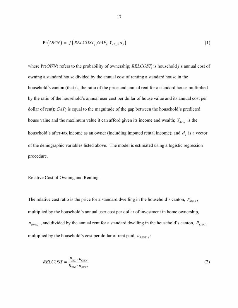
( ) ( ,Pr , , , )j j AT j jOWN f RELCOST GAP Y d= (1)
where Pr(OWN) refers to the probability of ownership; RELCOSTj is household j’s annual cost of
owning a standard house divided by the annual cost of renting a standard house in the
household’s canton (that is, the ratio of the price and annual rent for a standard house multiplied
by the ratio of the household’s annual user cost per dollar of house value and its annual cost per
dollar of rent); GAPj is equal to the magnitude of the gap between the household’s predicted
house value and the maximum value it can afford given its income and wealth; ,AT jY is the
household’s after-tax income as an owner (including imputed rental income); and jd is a vector
of the demographic variables listed above. The model is estimated using a logistic regression
procedure.
Relative Cost of Owning and Renting
The relative cost ratio is the price for a standard dwelling in the household’s canton, ,
multiplied by the household’s annual user cost per dollar of investment in home ownership,
, and divided by the annual rent for a standard dwelling in the household’s canton, ,
multiplied by the household’s cost per dollar of rent paid, :
,STD lP
R,OWN ju ,STD l
,RENT ju
STD OWN
STD RENT
P uRELCOSTR u
⋅=
⋅ (2)

18
where the household and locational subscripts (j and l, respectively) are omitted (henceforth we
will omit these subscripts from all equations). The standard prices and rents for each canton are
calculated from hedonic equations, holding the dwelling characteristics constant.7
The user cost of owner occupied housing in Switzerland is:
( )( ) ( )( ) ( ) ( )
( )( )
1 1 1 1 1
1
OWN Y UA E Y UA IA F Y Y W
K
u v i v v i
r
τ τ τ μ τ η
τ π
∗ ∗ ∗
∗
= − − + − + + − + + −
− − −
φ τ (3)
where is the annual user cost per dollar of investment in an owner-occupied house; OWNu Yτ is
the household’s tenure choice income tax rate taking into account federal, cantonal, and
communal rates; is the rate of return that could be earned on alternative investments of the
equity; is the present-value equivalent of the declining unamortized loan-to-value (LTV)
ratios over the expected holding period;
Ei
UAv∗
8 IAv∗ is the present-value equivalent of the indirectly
amortized LTV ratios over the expected holding period;9 is the mortgage interest rate (which
we assume here to be the same for first and second mortgages); μ is housing costs other than
mortgage interest, which are defined here to include maintenance, property taxes, and insurance
premiums; η is imputed rent as a fraction of house price;
Fi
φ is the proportion by which house
7 Further details about the hedonic and other estimations not reported here are available from the first author.
8 Assuming no inflation in house prices, a 10-year holding period, a discount rate of 3%, and amortization of 1% of
the value of the house each year, , where is the current unamortized LTV ratio. 0.53UA UAv v∗ = − UAv
9 For households that amortize only indirectly, , given the same assumptions as for (see
footnote 8). For households that amortize both directly and indirectly, the present value adjustment factor is
multiplied by the proportion amortized indirectly.
0.053IA IAv v∗ = + UAv∗

19
value is underestimated for purposes of wealth or property taxation; Wτ is the household’s tenure
choice wealth tax rate; Kτ∗
*IAv >
is the annualized capital gains tax rate; π is the expected rate of
capital gains in housing (net of depreciation); and r is a risk adjustment to expected capital gains.
The tenure choice income and wealth tax rates measure the tax advantage of owning relative to
renting; they are defined in more detail in the Appendix.
The first term on the right-hand side of Eq. (3) is the opportunity cost of equity, which is
after-tax because the returns to alternative investments would generally be taxed. The second
term is the after-tax (because it is deductible) cost of mortgage interest. Note that in the case of
indirect amortization ( ), the household continues to pay interest on both the unamortized
part of the mortgage and the indirectly amortized part. The third term refers to housing
expenses, which are all assumed to be deductible. The fourth, fifth, and sixth terms in Eq. (3)
refer to the imputed rent tax, the wealth tax adjusted for the undervaluation of housing wealth,
and the after-tax risk-adjusted expected capital gains rate, respectively.
0
10
Focusing now on the cost of rental housing, the annual user cost per dollar of market rent
paid, , equals 1, with two exceptions. As noted above, rent is partially deductible from
income for tax purposes in the cantons of Vaud and Basel Landschaft. In addition to the Vaud
and Basel Landschaft deductions, rents may be subsidized in all cantons for households that meet
certain criteria. Therefore, the rental user cost is:
RENTu
( )( ,11 Y CRENTu )τ ρθ −= − , (4)
10 We assume that households’ Troisième pilier contributions are independent of tenure choice and, therefore, that
indirect amortization does not affect the user cost of ownership except with respect to mortgage interest payments.

20
where θ is the proportion of the rent that is subsidized, is the household’s cantonal and
communal marginal income tax rate, and ρ is the amount of rent that can be deducted, expressed
here as a proportion of the rent paid.
,Y Ct
Borrowing Constraints
Mortgage underwriters impose both a wealth and an income constraint on borrowers. Previous
research has documented the impacts of borrowing constraints on home ownership rates
(Linneman and Wachter 1989; Haurin et al. 1997; Chiuri and Jappelli 2003). The wealth
constraint is defined as:
0.24W ≥ H
H
(5)
where W is the household’s liquid wealth and H is the value of the house the household desires to
purchase. This constraint requires a minimum 20% of the value of the house in equity, plus an
additional 4% of the value for closing costs, consisting mainly of transfer taxes. The income
constraint is defined as follows:
( )0.33 0.05 1.04 0.02Y H W≥ − + (6)
where Y is household income and the other terms are as defined above. As noted previously, this
assumes a 5% interest rate on the mortgage, amortization of 1% per year, and other housing

21
expenses (maintenance, property taxes, insurance, and so forth) of 1% per year.11 The
borrowing constraint gap is then defined for the purposes of estimating the tenure choice
equation as the maximum of the wealth and income constraint gaps, based on the househo
optimal or predicted house value ( H ), predicted liqu wealth (W ), and permanen inc
ld’s
id t ome ( ): Y
( )( )ˆ ˆ ˆ ˆ ˆ ˆmax 0.24 , 0.05 1.04 0.02 0.33GAP H W H W H Y= − − + − . (7)
Household Income and Other Variables
In addition to the relative cost ratio and borrowing constraint gap variables, the tenure choice
equation also includes a variable measuring after-tax income calculated as if each household
were an owner. This is hypothesized to have an effect on tenure choice independent of the other
two economic variables because the taste for privacy and control over domestic space may be a
function of income. This variable is income as an owner as calculated for the purposes of the
tenure choice income tax rate less the taxes that would be paid as an owner (see the Appendix for
further details on the calculation of these tax payments).
Demographic characteristics included in the model are marital status and age of the
household reference person and the number of dependent children in the household.12 Marital
status is specified as a series of dummy variables for single, divorced, and widowed persons,
with married being the default. The hypothesis is that married persons are most likely to be
homeowners and single persons least likely. The probabilities for divorced and widowed persons
11 The income constraint as defined here is a blend of the criteria of the two main mortgage lenders in Switzerland,
Credit Suisse and UBS.
12 We initially also included the gender of the household head, but this was not statistically significant.
22
should be between those for single and married persons. Age is also specified as a series of
dummy variables, in this case for four age groups, of which the youngest is the default. The
probability of ownership should increase with age, as individuals become more settled in their
careers and personal lives. Also, the addition of children to a household implies greater stability
and a desire for additional indoor and outdoor space that may be associated with ownership.
Endogeneity Issues
Bourassa (2000) shows that current income and wealth can be endogenous in a model of tenure
choice. Households may work more hours and save more if they decide to purchase a home.
Also, amortizing a mortgage builds up wealth in the form of home equity. For the latter reason,
it would seem that endogeneity would be particularly likely to be a problem with respect to
current wealth. In fact, we find that in Switzerland current liquid wealth for owners averages
nearly five times that for renters, while fitted or predicted liquid wealth from a regression of
current liquid wealth on selected household characteristics averages only twice as high for
owners as for renters. In contrast, current household income averages about 40% higher for
owners, while permanent household income (the fitted value from a regression of current
household income on household characteristics) averages about 30% higher. Thus it appears that
current liquid wealth is more likely to be endogenous than is current income.
To avoid potential endogeneity problems, we use predicted liquid wealth and permanent
household income to calculate the borrowing constraint gap (see Haurin et al. 1997 for another
example of this approach). We also use these variables to estimate and predict optimal house
values and we use permanent income in the optimal rent equation estimated for Vaud and Basel.
The optimal house values are used when calculating the borrowing constraint gap and loan-to-

23
value ratios. We use permanent salary income to predict Deuxième and Troisième pilier
contributions, and predicted liquid wealth in the calculation of LTV ratios. Predicted liquid
wealth is also the basis for our tenure choice wealth tax rate calculations.
We use a somewhat different approach for calculating the tenure choice income tax rates
that are part of the user cost in the numerator of the relative cost ratio and for after-tax income as
an owner. Here, because endogeneity is not likely to be as much of an issue, we start out with
actual incomes but use predicted house values and LTV ratios to estimate how households’
incomes would differ if they owned rather than rented. As discussed in the Appendix, for current
owners we convert income as an owner to income as a renter by adding an estimate of the actual
return to home equity. Then, to obtain income as an owner, we subtract the return from home
equity—calculated using optimal (predicted) house values and predicted LTV ratios—from
income as a renter.
The multi-stage estimation process that we implement in response to the potential
endogeneity problems raises questions about identification and standard errors. We rely on
functional form (logit versus OLS) to insure that the structural tenure choice equation is
identified. We use bootstrapping to calculate more accurate standard errors. Bootstrapping
involves repeated sampling with replacement from a sample of data to produce a distribution of
estimates which can then be used to calculate standard errors and other statistics (Efron and
Tibshirani 1993; Mooney and Duval 1993). The multi-stage estimation process used here may
result in standard errors that are too small, particularly with respect to the borrowing constraint
gap variable, the calculation of which depends directly on the results of other estimations.
Consequently, we bootstrap the entire system of equations that feed into the borrowing constraint
gap and report the resulting standard errors rather than the ones from the non-bootstrapped tenure
choice estimation.
24
Data and Analysis
Data
Our primary data source is the 1998 Enquête sur les revenus et la consommation. Of the 9,295
households participating in the survey nationwide, 3,588 were located in the cantons we focus on
here, had sufficient data for analysis, and satisfied our requirement that the household reference
person be of working age (between 18 and 65) and in the labor force. The survey provides
detailed information about household revenues and their sources as well as details regarding
household expenses and household characteristics.
The survey does not document household wealth, although it does provide indirect
information about wealth by recording details about income from wealth. Here we use income
from selected sources to impute liquid wealth, using as a discount rate. Also, no information
is provided about the value of owner-occupied dwellings. However, characteristics of the
dwellings are provided, and we were able to obtain hedonic estimates of the dwellings’ values
from the Centre d’Information et de Formation Immobilières SA (CIFI), a commercial property
valuation firm in Zurich.
Ei
Means for the variables in the tenure choice equations are shown in Table 2. The data for
Basel are weighted averages for the two Basel half-cantons. Compared to the sample as a whole,
ownership rates are relatively high in Berne and low in Geneva. After-tax income is fairly
comparable across locations, but the relative cost of owning and renting is high in Zurich and
Geneva and low in Berne. The borrowing constraint gap is low in Berne, Basel, and Vaud, and
high in Zurich and Geneva. Demographic characteristics are fairly constant across cantons,
although household reference persons in Berne and Vaud are more likely to be married and to

25
have children, while household reference persons in Zurich and Geneva are more likely to be in
the youngest and oldest age groups.
[Table 2 here]
The last two columns of Table 2 compare owners with renters. Owners have higher
incomes and lower relative cost ratios than renters. On average, owners have a negative
borrowing constraint gap (that is, the average household has more liquid wealth than needed to
purchase the optimal house), while renters have a positive gap. Owners are much more likely
than renters to be married and much less likely to be in the youngest age group. Owners also
have more children on average.
Table 3 provides additional details about the relative cost ratios calculated for all
households (current owners and renters) in the sample. Geneva, which has the highest average
relative cost ratio, also has the highest standard house value and price-rent ratio. On the other
hand, it has the lowest average user cost of owner-occupied housing, due to high income tax
rates and low imputed rents.13 Geneva households also have by far the lowest rental cost factor,
due to the fact that they are much more likely to receive rental subsidies. These subsidies would
reduce average rents by nearly 7%.14 Rent deductions from income for taxation purposes that
are available in Basel and Vaud reduce rental costs there by about 8% and 10%, respectively.15
[Table 3 here]
13 The Swiss user costs are similar in magnitude to those reported by Himmelberg et al. (2005) for U.S. cities in
2004.
14 We estimated a logit model to predict the probability of receiving a rental subsidy, and the likelihood of receiving
rental subsidies is so low in the other cantons that the model predicts that none of the households in our sample in
those cantons would receive such a subsidy.
15 The mean reduction for Basel is the weighted average deduction after applying the rules for Basel Landschaft
(which allows a deduction) and Basel Stadt (which does not).
26
In addition to the user cost variables and parameters listed in Table 3, Eq. (3) includes
two interest rates and a risk-adjusted expected capital gains rate. The rate of interest that would
be earned on alternative investments of home equity, , is set at 0.03, which is the rate for
medium-term bank notes issued by large banks as reported by the Swiss National Bank (2006b)
for 1998. The mortgage interest rate, , set at 0.04, is also based on Swiss National Bank
(2006b) statistics. We assume that the risk-adjusted capital gains rate,
Ei
Fi
rπ − , is 0, given that
there was considerable uncertainty about future house price movements in 1998.
Geneva also stands out in the statistics on borrowing constraints (Table 4). In addition to
having by far the largest borrowing constraint gap, it also has the highest mean optimal house
value and the highest percentage of households that are either wealth or income constrained. In
contrast, in Berne, where house prices are relatively low, households are much less likely to be
either wealth or income constrained.
[Table 4 here]
Optimal House Value and Rent Estimations
The optimal house value equation is estimated for current owners by regressing hedonic
estimates of their dwelling values on the user cost of owner-occupied housing, permanent
household income, predicted liquid wealth, the number of children in the household, and dummy
variables for the cantons. The user cost is identical to the user cost in Eq. (3), except for the fact
that marginal tax rates are substituted for tenure choice tax rates. We then use this equation to

27
predict optimal house values for the entire sample.16 These values are then used to estimate LTV
ratios, user costs, relative cost ratios, and borrowing constraint gaps, which are in turn used to
estimate the tenure choice equation. The user cost was not significant, so it was omitted from the
final estimation.
A simple optimal rent equation was estimated for Basel and Vaud for the purposes of
calculating ρ, the rent deduction as a proportion of optimal rent. The dependent variable is the
actual annual rent paid by current renters, and the independent variables are permanent income
and the number of children. This equation is then used to predict optimal rents for all households
in Vaud and Basel.
Loan-to-Value Ratio Estimations
We model LTV ratios as a function of a hypothetical LTV ratio that assumes that all liquid
wealth is invested in the home before investing in any other asset ( HYPv
COTP
) plus a variable
measuring the amount of the annual Troisième pilier contribution ( ). Our estimation of the
LTV ratio equation shows that the actual LTV ratio is virtually the same as the hypothetical ratio
except when the household contributes to a Troisième pilier:
N
16 Following Haurin et al. (1997), Green and Vandell (1999), and others, we initially applied Heckman’s (1979) two-
stage sample selection bias method to address the fact that we are using estimations based on owners to make
predictions about renters. It was evident, however, that the inverse Mills ratio calculated from the first stage tenure
choice equation was collinear with variables in the optimal house value, optimal rent, and loan-to-value ratio
equations. As pointed out by a referee, the same variables that explain tenure choice are also likely relevant to these
other factors, thus calling into question the appropriateness of the two-stage technique in these cases. Note that
Haurin et al. (1997) concluded that there was no sample selection bias in their study. In any case, controlling for
sample selection bias has only a trivial impact on the tenure choice estimates and simulation results.

28
5
5
0.010 0.106 102
1.011 1.369 10 ,
. 0.788, 996.
HYP CONv v TP
Adj R n
−
−
×= + ×
= = (8)
Here , where and are the current unamortized and indirectly amortized LTV
ratios. We deliberately omit the constant term from this model. We use this model to predict
for all households, but use predicted liquid wealth and optimal house values to calculate
UA IAv v v= + UAv IAv
v
ˆHYPv a
predictions from an OLS regression to calculate COTP en ˆ ˆUAv v
nd
ThN . 1.011 HYP= and
enure Choice Estimations
he tenure choice estimates are shown in Table 5. As noted above, the reported standard errors
The
ˆIAv = v − UAv .
T
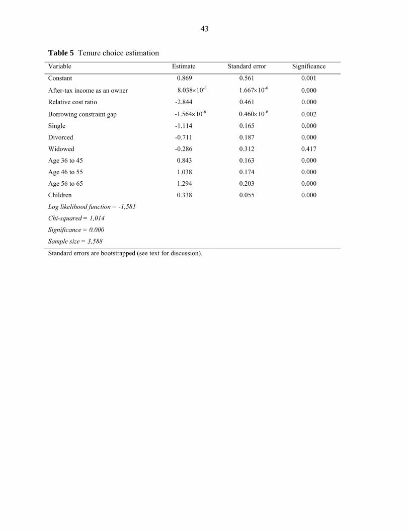
T
are bootstrapped.17 The results are as expected, with all but one of the estimates (the dummy
variable for widowed persons) significant at better than the 0.01% level. The probability of
ownership is positively related to after-tax income as an owner and negatively related to the
relative cost of owning and renting and to the borrowing constraint gap. Single household
reference persons are least likely to be owners, followed by divorced and widowed persons.
likelihood of ownership increases with age and with the number of children in the household.
17 Generally, bootstrapping has a small impact on the standard errors, although the bootstrapped standard error for
the gap variable is somewhat higher than the non-bootstrapped standard error (0.460 × 10⁻⁶ versus 0.289 × 10⁻⁶).
The bootstrapped results are based on 100 random samples with replacement of the same size as the original sample
(n = 3,588).

29
The estimates shown in Table 5 are then used together with modified variable values for the
purposes of simulating hypothetical changes.
[Table 5 here]
Simulation of Changes in Tax Policy, Underwriting Standards, and Price Levels
We simulate a number of hypothetical changes as a means for answering the question posed by
the title of this article (Table 6). These simulations are partial in the sense that we do not attempt
to model general equilibrium effects.18 We report bootstrapped confidence intervals around the
simulated ownership rates; in all cases these are fairly narrow and in all but one case (elimination
of rent subsidies) they suggest that the hypothetical change in ownership rates is statistically
significant.19
We first simulate the impacts of relaxing wealth and income constraints, both separately
and together. Reducing the down payment constraint from 24% to 14% (10% plus 4% closing
costs) or 9% would in each case increase the ownership rate by about 1 percentage point (from
26.9% to 28.0%), reflecting the fact that these constraints would continue to be binding for many
households. Relaxing the income constraint to allow mortgage principal, interest, and other
expenses to be as much as 40% of gross income rather than 33% has a similarly small impact.
18 A similar approach is used to simulate impacts of hypothetical changes in tax and subsidy policies on home
ownership in the U.S. in Bourassa and Yin (2006; 2008).
19 To bootstrap each simulated ownership rate we take 1,000 random samples with replacement of the same size as
the original sample. The bootstrapped distribution is then centered on our simulated ownership rate and the
estimated ownership rates corresponding to cumulative probabilities 0.025 and 0.975 are the lower and upper
bounds, respectively, of the 95% confidence interval.

30
However, relaxing the down payment constraint to 14% while also relaxing the income
constraint to 40% would raise the ownership rate by about 3 percentage points.
[Table 6 here]
We next simulate the effects of eliminating the tax on imputed rent with and without also
removing the deductions for mortgage interest and other housing expenses. Removing the
imputed rent tax while retaining the deductions increases the ownership rate by 9 percentage
points. Removing both the tax and the deductions reduces the ownership rate by about 1
percentage point, reflecting the fact that mortgage interest and other housing expenses on
average exceed imputed rent.
As mentioned above, eliminating rent subsidies (θ = 0) would have virtually no impact on
the ownership rate, although eliminating rent controls would increase the ownership rate by over
2 percentage points by making renting less attractive relative to owning. We simulate the
elimination of rent controls by setting the duration of tenancy variable in the hedonic rent models
to zero (rather than to its mean) for the purposes of calculating the standard rent ( STDR ) for each
canton. This assumes that initial rents are at market and that rent controls operate mainly to limit
rent increases after a dwelling is occupied. General equilibrium effects would be smaller than
our results suggest if the supply of rental housing expanded and market rents dropped due to
elimination of rent controls. Also, part of the discount due to duration of tenancy may be due to
normal market functioning (it is cheaper to retain a good tenant than to search for a new one).
Again, this suggests that we may be overestimating the impacts of rent controls. If we eliminate
all benefits to renters—including subsidies, controls, and income tax deductions—our partial
analysis suggests that the ownership rate increases by less than 3 points, although general
equilibrium analysis would probably find a smaller effect.
31
The last set of simulations involves changes in price levels and price-rent ratios. If prices
and price-rent ratios drop by 10%, the ownership rate increases by 6 points. If this change is
combined with relaxation of the down payment constraint to 14% and the income constraint to
40%, then the ownership rate increases by about 10 points. We then simulate a more dramatic
change in prices and price-rent ratios by dropping prices by 20%, which is the approximate
difference between the mean price-rent ratios in Geneva and Berne (note that our standard house
price for Geneva is nearly 50% greater than that in Berne). This 20% drop in prices and ratios
results in about a 13 percentage point increase in the ownership rate, to over 40%.
Finally, we simulate a combination of changes designed to make the Swiss situation
somewhat more like that in the U.S. (in 1998). Prices and price-rent ratios drop by 20%, the
imputed rent tax is eliminated, and the wealth constraint is relaxed to 9% (5% down payment
plus 4% closing costs). When eliminating the imputed rent tax, we retain the mortgage interest
deduction and the deduction for other housing expenses, which is worth about as much in
Switzerland as the property tax deduction is worth in the U.S. (about 1% of house value). This
combination of changes results in a nearly 23 point increase in the ownership rate, to 49.5%.
Given the individual results for reducing prices, eliminating the imputed rent tax, and relaxing
the wealth constraint, this result is due primarily to the reduction in prices. Elimination of the
tax on imputed rent is responsible for most of the balance of the change, with only a small
impact due to the reduction in the wealth constraint.

32
Conclusions
Switzerland’s low rate of home ownership is attributable to the fact that prices are very high
relative to household incomes and wealth. Another important factor is the tax on imputed rent;
however, if the deductions for mortgage interest and other housing expenses were removed along
with the imputed rent tax, the effect would be to reduce, rather than increase, the ownership rate.
A combination of lower prices (and price-rent ratios), elimination of the imputed rent tax, and
reduction in the wealth constraint to 9% of house value would raise the ownership rate for the
Swiss cantons studied here to nearly 50%.
Swiss-style house prices and home ownership rates can certainly be found in the more
costly parts of other countries, including the U.S. To use one of that country’s most expensive
cities as an example, the 2000 U.S. census reports that median house prices in the City of San
Francisco were $396,400, or about SFr. 574,500 (using the 1998 exchange rate), which is
comparable to our standard price for Geneva. San Francisco’s home ownership rate in 2000 was
35%, while the national rate was about 66%. Glaeser and Gyourko (2003) show that San
Francisco has the highest land costs in the nation, and they attribute that largely to land use
constraints, although topography is obviously also a factor.
Similarly, house prices are high in Switzerland mainly because land prices are high.
Land prices are high because there is relatively little developable land, both for topographical
reasons and because the Swiss attach considerable importance to conservation of both
agricultural landscapes and urban heritage. Although a large majority of households would
prefer home ownership in Switzerland, the country has a tradition of long-term rental tenancy. It
seems unlikely that the Swiss would support a substantial expansion of the ownership rate if that
came at the expense of environmental quality or the current system of supports for renters.
33
Consequently, it seems likely that Swiss ownership rates will remain low into the foreseeable
future.
Acknowledgments The authors thank Peter Bolliger (Swiss Statistical Office) for providing the
household survey data, Donato Scognamiglio and Philippe Sormani (CIFI) for calculating the
hedonic estimates of house values, Séverine Cauchie and Céline Kuhn for collecting the tax and
subsidy data, and Jörg Baumberger, Philippe Thalmann, and an anonymous referee for helpful
comments.
References
Aebersold, A. (1994). Miete oder Eigentum? Die ökonomische Entscheidung über den
Wohnungsbesitz. Hallstadt, Switzerland: Rosch-Buch.
Bourassa, S. C. (2000). Ethnicity, endogeneity, and housing tenure choice. Journal of Real
Estate Finance and Economics, 20(3), 323–341.
Bourassa, S. C., & Grigsby, W. G. (2000). Income tax concessions for owner-occupied housing.
Housing Policy Debate, 11(3), 521-546.
Bourassa, S. C., & Yin, M. (2006). Housing tenure choice in Australia and the United States:
impacts of alternative subsidy policies. Real Estate Economics, 34(2), 303-328.
Bourassa, S. C., & Yin, M. (2008). Tax deductions, tax credits, and the home ownership rate of
young urban adults in the United States. Urban Studies, 45(5/6), 1141–1161.
Bureau d’information fiscale (2003). Les droits de mutation. Berne, Switzerland.

34
Bureau d’information fiscale (2005). L’impôt sur le revenu des personnes physiques. Berne,
Switzerland.
Bureau d’information fiscale (2006a). Les impôts en vigueur de la Confédération, des cantons et
des communes. Berne, Switzerland.
Bureau d’information fiscale (2006b). L’impôt sur la fortune des personnes physiques. Berne,
Switzerland.
Chiuri, M. C., & Jappelli, T. (2003). Financial market imperfections and home ownership: a
comparative study. European Economic Review, 47(5), 857–875.
Commission intercantonale d’information fiscale (1999). L’imposition de la valeur locative.
Berne, Switzerland.
Commission intercantonale d’information fiscale (2000). L’impôt sur les gains immobiliers.
Berne, Switzerland.
Credit Suisse (2005). Real estate bubble in Switzerland? Economic Research Spotlight
(December).
Cuennet, S., Favarger, P., & Thalmann, P. (2002). La politique du logement. Lausanne,
Switzerland: Presses polytechniques et universitaires romandes.
Efron, B., & Tibshirani, R. J. (1993). An introduction to the bootstrap. New York: Chapman &
Hall.
Glaeser, E. L., & Gyourko, J. (2003). The impact of building restrictions on housing
affordability. Economic Policy Review (June), 21–39.
Goodman, A. C. (1990). Demographics of individual housing demand. Regional Science and
Urban Economics, 20(1), 83–102.

35
Green, R. K., & Vandell, K. D. (1999). Giving households credit: how changes in the U.S. tax
code could promote homeownership. Regional Science and Urban Economics, 29(4), 419–
444.
Haurin, D. R., Hendershott, P. H., & Wachter, S. M. (1997). Borrowing constraints and the
tenure choice of young households. Journal of Housing Research, 8(2), 137–154.
Heckman, J. J. (1979). Sample selection bias as a specification error. Econometrica, 47(1), 153–
161.
Hendershott, P. H., & J. Slemrod (1983). Taxes and the user-cost of capital for owner-occupied
housing. Journal of the American Real Estate and Urban Economics Association, 10(4),
375–393.
Himmelberg, C., Mayer, C., & Sinai, T. (2005). Assessing high house prices: bubbles,
fundamentals and misperceptions. Journal of Economic Perspectives, 19(4), 67-92.
Linneman, P. (1985). An economic analysis of the homeownership decision. Journal of Urban
Economics, 17(2), 230-246.
Linneman, P., & Wachter, S. M. (1989). The impacts of borrowing constraints on
homeownership. Journal of the American Real Estate and Urban Economics Association,
17(4), 389–402.
Mooney, C. Z., & Duval, R. D. (1993). Bootstrapping: a nonparametric approach to statistical
inference. Newbury Park, CA: Sage Publications.
Office fédéral du logement (2004). Encouragement à la propriété du logement au moyen de la
prévoyance professionnelle. Berne, Switzerland.
Office fédéral de la statistique (1999). Enquête sur les revenus et la consommation 1998: bases.
Neuchâtel, Switzerland.

36
Office fédéral de la statistique (2007). Indice suisse des prix à la consommation: loyer du
logement. Available at <http://www.statistik.admin.ch/> (March).
Swiss National Bank (2006a). Real estate price indices. Monthly Statistical Bulletin. Available at
<http://www.snb.ch/> (June).
Swiss National Bank (2006b). Interest rates on bank deposits and mortgages. Monthly Statistical
Bulletin, available at <http://www.snb.ch/> (September).
Thalmann, P. (1987). Explication empirique des loyers lausannois. Swiss Journal of Economics
and Statistics, 123(1), 47–70.
Thalmann, P. (1999). Which is the appropriate administrative level to promote home ownership?
Swiss Journal of Economics and Statistics, 135(1), 3–20.
Thalmann, P., & Favarger, P. (2002). Locataires ou propriétaires? Enjeux et mythes de
l’accession à la propriété en Suisse. Lausanne, Switzerland: Presses polytechniques et
universitaires romandes.
U.S. Census Bureau (2004). American Housing Survey for the United States, Current Housing
Reports, Series H150/03. Washington, DC: U.S. Government Printing Office.
Werczberger, E. (1997). Home ownership and rent control in Switzerland. Housing Studies,
12(3), 337–353.

37
Appendix: Tenure Choice Tax Rates
The tenure choice income tax rate measures the tax advantage (or disadvantage) of
owning relative to renting and is an average rather than a marginal rate (Hendershott and
Slemrod 1983). In the case of Switzerland, it is generally defined as:
( ) ( )( ), ,
ˆ 1Y RENT Y OWN
YUA E UA IA F
T T
H v i v v iτ
μ η∗ ∗ ∗
−=
− + + + − (A1)
where is the federal and cantonal (including communal and church) income tax a
household would pay if it rented; is the income tax it would pay if it owned a dwelling of
value H; and the other terms are as defined previously. The denominator in Eq. (A1) is the
change in taxable income when a household shifts from renting to owning.
,Y RENTT
,Y OWNT
The procedure for calculating the tenure choice tax rate is as follows. In the case of
current owners, taxable income as a renter is calculated by adding the return to actual home
equity, , to actual income. Here H is the value of each homeowner’s house and
is the homeowner’s current unamortized LTV ratio. Taxable income as an owner is then
calculated for renters and recalculated for owners as taxable income as a renter less a predicted
return to home equity, , where is the household’s “optimal” house value and
is the predicted current LTV ratio. Then all of the applicable housing and other deductions are
applied to income as a renter and as an owner before calculating the tax payments and
, which are then inserted into Eq. (A1).
( )1 UA EH v i− UAv
UAv( )ˆ ˆ1 UA EH v i− H
,Y RENTT
,Y OWNT
As noted above, the denominator in Eq. (A1) represents the change in taxable income if

38
the household rented rather than owned. Additions to taxable income are the return to home
equity, deductible mortgage interest payments, and maintenance and other deductible housing
expenses. Imputed rent is a reduction from taxable income. For households in Vaud, where
imputed rent is partially deductible, only the nondeductible portion of η affects cantonal tax
liability. In the case of Geneva, expenses are not deductible at the cantonal level, so μ enters into
Eq. (A1) only to the extent that it affects federal income tax liability. For households in Vaud
and Basel Landschaft, where rent is at least partly deductible from income for cantonal income
tax purposes, the difference in taxable income also takes into account the deductible portion of
rent paid.
Similar considerations apply to the wealth tax rate:
, ,
ˆW RENT W OWN
W
T TH
τφ−
= (A2)
where and are the wealth taxes the household would pay as a renter and as an
owner, respectively. Here the denominator is the increase in the wealth tax base if the household
rents rather than owns, which is due to the fact that housing wealth is undervalued for tax
purposes.
,W RENTT ,W OWNT

39
Table 1 Ownership rates for selected European, North American, and Australasian
countries
Country % Country %
Romania 91.6 New Zealand 67.8
Hungary 90.9 United States 66.2
Lithuania 84.9 Luxembourg 66.1
Spain 82.1 Canada 66.1
Slovenia 81.5 Finland 63.5
Ireland 76.9 Belgium 63.1
Norway 76.7 Latvia 59.6
Portugal 74.8 Poland 58.9
Slovakia 73.6 France 54.7
Estonia 72.2 Netherlands 50.4
Greece 71.7 Austria 48.7
Italy 71.2 Liechtenstein 48.1
Australia 69.5 Czech Republic 47.1
United Kingdom 68.0 Germany 42.0
Cyprus 68.0 Switzerland 33.6
Sources: European Commission (http://epp.eurostat.ec.europa.eu); Australian Bureau of Statistics
(http://www.abs.gov.au); Statistics Canada (http://www.statcan.ca); Statistics New Zealand
(http://www.stats.govt.nz); and United States Bureau of the Census (http://www.census.gov). Data are
from the most recent census prior to 2002.

40
Table 2 Tenure choice variable means Variable
Zurich
Berne
Basel
Vaud
Geneva
Full sample
Owners
Renters
Owner (%) 24.9 35.5 25.7 26.5 10.3 26.9 100.0 0.0
After-tax income as an owner ( ATY ) (SFr.)
94,614
79,151
87,641
92,157
86,364
88,368
112,404
79,538
Relative cost ratio (RELCOST)
1.27
1.07
1.14
1.14
1.38
1.18
1.14
1.20
Borrowing constraint gap (GAP) (SFr.)
152,259
–40,325
67,546
20,269
200,995
68,635
–108,452
133,697
Marital status of reference person (%)
Married 50.2 57.3 52.2 58.9 49.9 54.0 83.2 43.3
Single 35.5 28.8 32.6 27.5 36.0 31.8 7.5 40.8
Divorced 12.9 12.0 13.0 12.0 12.8 12.5 6.8 14.6
Widowed 1.4 1.9 2.2 1.6 1.3 1.7 2.5 1.3
Age of reference person (%)
18 to 35 38.2 35.7 33.1 36.4 41.0 36.8 11.3 46.2
36 to 45 27.8 28.5 30.3 30.1 24.1 28.4 34.5 26.1
46 to 55 21.5 24.1 25.5 21.7 21.1 22.7 33.3 18.8
56 to 65 12.5 11.7 11.1 11.8 13.8 12.1 20.9 8.9
Number of children
0.58
0.68
0.54
0.72
0.58
0.63
0.94
0.51
Sample size 1,237 1,015 452 605 279 3,588 998 2,590
All sample data are weighted so that they more accurately reflect the populations from which they are drawn.
We use household weights calculated by the Swiss Statistical Office. In 1998, SFr. 1.00 ≈ US$ 0.69.

41
Table 3 Relative cost ratio variable means and parameters Variable
Zurich
Berne
Basel
Vaud
Geneva
Full sample
Relative cost ratio (RELCOST)
1.27
1.07
1.14
1.14
1.38
1.18
Standard house value (PSTD) (SFr.)
510,617
364,962
455,457
392,252
542,210
444,382
Standard annual rent (RSTD) (SFr.)
18,613
15,268
18,634
16,431
18,810
17,303
Price-rent ratio (PSTD/RSTD) 27.4 23.9 24.4 23.9 28.8 25.6
User cost (uOWN) 0.046 0.045 0.046 0.047 0.044 0.046
Tenure choice income tax rates
Combined ( Yτ ) 0.245 0.286 0.280 0.240 0.307 0.265
Federal ( ,Y Fτ ) 0.059 0.048 0.055 0.053 0.054 0.054
Cantonal ( ,Y Cτ ) 0.187 0.238 0.226 0.187 0.253 0.211
Tenure choice wealth tax rate ( Wτ )
0.001
0.002
0.002
0.003
0.002
0.002
Unamortized LTV ( ) UAv∗ 0.743
0.657
0.714
0.697
0.757
0.709
Indirectly amortized LTV ( IAv∗ )
0.041
0.049
0.045
0.046
0.039
0.044
Cantonal taxable imputed rent as a proportion of house value (η )
0.035
0.030
0.032
0.035
0.018
0.032
Cantonal wealth tax discount (φ )
0.300
0.400
0.360
0.300
0.400
0.344
Rental cost ( RENTu ) 1.000 1.000 0.982 0.993 0.933 0.990
Subsidy as a proportion of rent (θ)
0.000
0.000
0.000
0.000
0.067
0.006
Cantonal income tax deduction as a proportion of rent (ρ)
0.000
0.000
0.082
0.102
0.000
0.030
Cantonal tax rates include communal and church rates.

42
Table 4 Borrowing constraint gap variable means Variable
Zurich
Berne
Basel
Vaud
Geneva
Full sample
Borrowing constraint gap (GAP) (SFr.)
152,259
–40,325
67,546
20,269
200,995
68,635
Optimal house value ( H ) (SFr.)
605,444
421,406
523,032
454,701
654,789
520,844
Predicted liquid wealth ( ) (SFr.) W
134,858
137,231
134,961
128,173
134,762
134,213
Permanent household income ( ) (SFr.) Y
104,823
105,645
104,793
103,875
105,003
104,875
Wealth constrained (%) 62.2 40.2 53.3 48.2 61.5 52.4
Income constrained (%) 61.2 16.7 37.9 24.5 71.0 40.1
Either wealth or income constrained (%)
64.9
40.2
53.7
48.2
72.9
54.3
43
Table 5 Tenure choice estimation Variable Estimate Standard error Significance
Constant 0.869 0.561 0.001
After-tax income as an owner 8.038×10⁻⁶ 1.667×10⁻⁶ 0.000
Relative cost ratio -2.844 0.461 0.000
Borrowing constraint gap -1.564×10⁻⁶ 0.460×10⁻⁶ 0.002
Single -1.114 0.165 0.000
Divorced -0.711 0.187 0.000
Widowed -0.286 0.312 0.417
Age 36 to 45 0.843 0.163 0.000
Age 46 to 55 1.038 0.174 0.000
Age 56 to 65 1.294 0.203 0.000
Children 0.338 0.055 0.000
Log likelihood function = -1,581
Chi-squared = 1,014
Significance = 0.000
Sample size = 3,588
Standard errors are bootstrapped (see text for discussion).

44
Table 6 Simulation results Simulation
Simulated ownership rate (%)
Bootstrapped 95% confidence intervals
Relax down payment constraint to 14% (10% plus closing costs) 28.0 27.2–28.7
Relax down payment constraint to 9% (5% plus closing costs) 28.0 27.3–28.8
Relax income constraint to 40% 28.1 27.4–28.9
Relax down payment constraint to 14% and income constraint to 40% 30.3 29.5–31.1
Eliminate tax on imputed rent 36.2 35.3–37.1
Eliminate tax on imputed rent and mortgage interest and housing expense deductions 25.8 25.0–26.6
Eliminate rent subsidies ( 0θ = ) 27.1 26.4–27.8*
Eliminate rent controls 29.0 28.2–29.9
Eliminate rent subsidies ( 0θ = ), rent controls, and rent deductions ( 0ρ = ) 29.4 28.6–30.2
House prices and price-rent ratios drop by 10% 33.3 32.5–34.1
House prices and price-rent ratios drop by 10%, down payment constraint is relaxed to 14%, and income constraint is relaxed to 40% 36.8 35.9–37.7
House prices and price-rent ratios drop by 20% 40.1 39.2–41.1
House prices and price-rent ratios drop by 20%, imputed rent tax is eliminated, and down payment constraint is relaxed to 9% 49.5 48.6–50.5
* The actual (weighted) ownership rate in the sample (26.9%) is within the confidence interval.