Embed Size (px)
Citation preview
University of PortoFaculty of Engineering
Analytical and Experimental Study on the Evolution ofResidual Stresses in Composite Materials
Jorge Borges de Almeida
Mechanical Engineer
A Thesis presented to the
Faculty of Engineering of the University of Porto
In partial fulfillment of the requirements for the Master of Science Degree in
Mechanical Engineering
Supervisor
Professor Doutor Pedro M. P. R. C. CamanhoAssessor
Professor Doutor António Torres Marques
Porto, September 20, 2005
Abstract
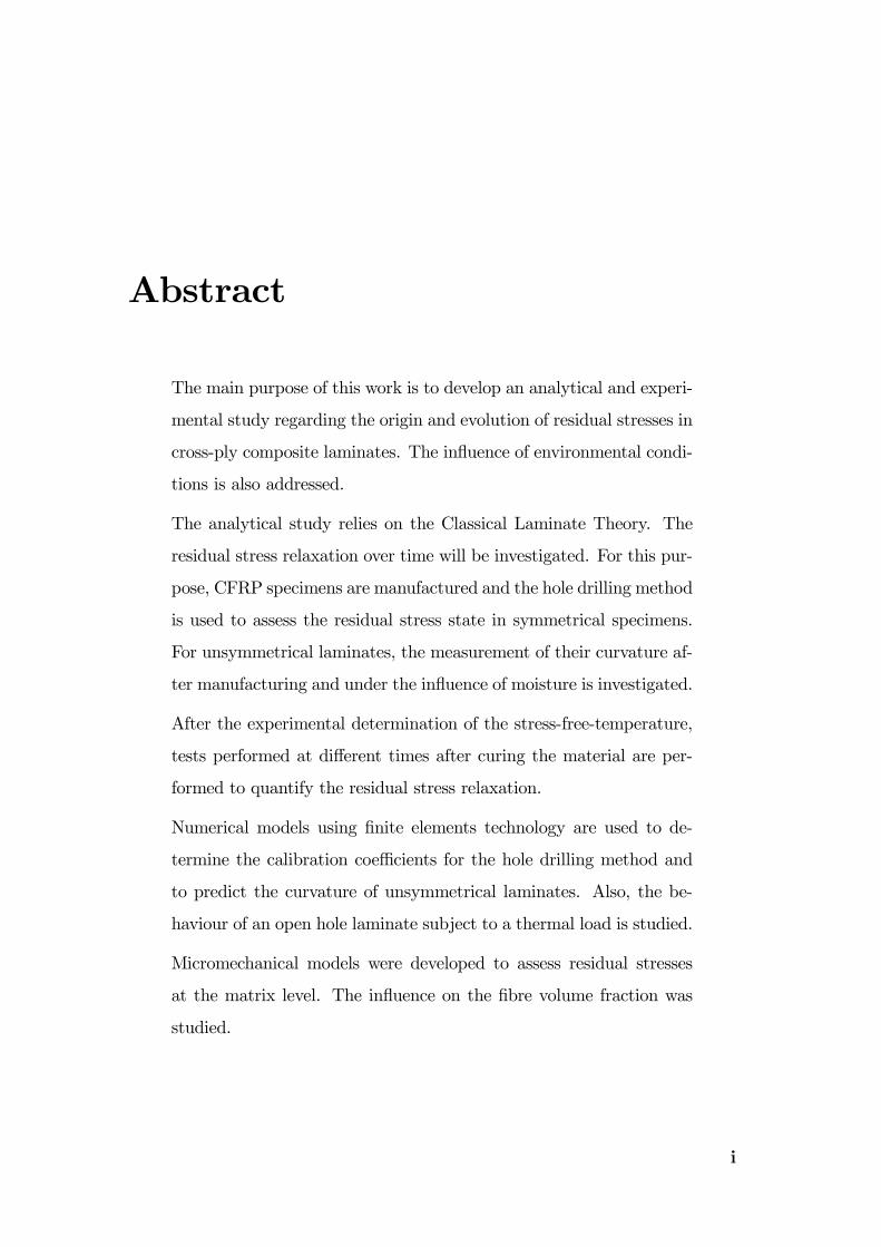
The main purpose of this work is to develop an analytical and experi-
mental study regarding the origin and evolution of residual stresses in
cross-ply composite laminates. The influence of environmental condi-
tions is also addressed.
The analytical study relies on the Classical Laminate Theory. The
residual stress relaxation over time will be investigated. For this pur-
pose, CFRP specimens are manufactured and the hole drilling method
is used to assess the residual stress state in symmetrical specimens.
For unsymmetrical laminates, the measurement of their curvature af-
ter manufacturing and under the influence of moisture is investigated.
After the experimental determination of the stress-free-temperature,
tests performed at different times after curing the material are per-
formed to quantify the residual stress relaxation.
Numerical models using finite elements technology are used to de-
termine the calibration coefficients for the hole drilling method and
to predict the curvature of unsymmetrical laminates. Also, the be-
haviour of an open hole laminate subject to a thermal load is studied.
Micromechanical models were developed to assess residual stresses
at the matrix level. The influence on the fibre volume fraction was
studied.
i

ii
Resumo
O objectivo principal deste trabalho é desenvolver um estudo analítico
e experimental relacionado com a origem e evolução de tensões residu-
ais em laminados compósitos cruzados. A influência de certas condições
ambientais será estudada.
O estudo analítico baseia-se na Teoria Clássica dos Laminados. A re-
laxação de tensões ao longo do tempo é investigada. Para tal, provetes
em carbono-epóxido são fabricados e o método do furo será usado para
avaliar o estado de tensões residuais nos provetes simétricos. Para o
caso dos provetes assimétricos, o estudo baseia-se na medição da re-
spectiva curvatura após cura e sob a influência de humidade.
Após a determinação experimental da temperatura correspondente
ao estado livre de tensões internas do material, são conduzidos testes
em diferentes ocasiões após a cura do material para quantificar o
relaxamento das tensões.
Métodos numéricos baseados na tecnologia dos elementos finitos são
igualmente usados para a determinação dos coeficientes de calibração
do método do furo. O comportamento de um provete de furo aberto
sujeito a uma carga térmica é também estudado.
Foram desenvolvidos modelos micromecânicos para avaliar tensões
residuais ao nível da matriz. A influência da fracção volúmica da
fibra foi estudada.
iii

iv
Zusammenfassung
Der Hauptzweck dieser Arbeit ist, die Entwicklung von Eigenspan-
nungen in gekreuzte Laminaten durch analytische und experimentelle
Weisen zu studieren. Der Einfluß von Klimabedingungen wird auch
adressiert.
Das CLT-Rechenverfahren wird angewendet. Die mögliche überzeitliche
Entspannung der Eigenspannungen wird untersucht. Für diesen Zweck
werden CFRP Laminaten hergestellt und die Bohrungmethode wird
angewendet, um die Eigenspannungen in den symmetrischen Lami-
naten festzustellen. Nach der Herstellung von unsymmetrischen Lam-
inaten wird die Biegung gemesst und mit numerischen Ergebnissen
verglischen. Ihre Entwicklung unter den Einfluss von Feuchtigkeit
wird auch erforscht.
Nach der Feststellung der spannungsfrei Temperatur des Werkstoffes,
werden verschiedene Tests überzeitlich durchgeführt, um die Entspan-
nung des Werkstoffes zu quantifizieren.
Durch die Technik der finite Elemente, werden die Biegungen der
unsymmetrischen Laminaten und die Calibrationskoeffizienten für die
Bohrungmethode festgestellt.
Das Verhalten einer Platte mit einem Loch unter den Einfluss einer
termischen Ladung wir auch untersucht.
Micromechanische Modellen wurden entwickelt, um die Eigenspan-
nungen am Matrixniveau festzustellen. Der Einfluß des Faseraus-
v

gabenbruches wurde studiert.
vi
Resumeé
Le but principal de ce travail est développer une étude analytique et
expérimentale concernant l’origine et l’évolution des efforts résiduels
dans des composites stratifiés. L’influence des conditions environ-
nementales est également adressée.
L’étude analytique se fonde sur la théorie classique des stratifiés. Le
temps fini de relaxation résiduelle d’effort sera étudié. À cette fin,
les spécimens de CFRP sont manufacturés et la méthode du trou
incrémental est employée pour évaluer l’état résiduel d’effort dans les
spécimens symétriques. Pour les stratifiés non symétriques, la mesure
de leur courbure après la fabrication et sous l’influence de l’humidité
est étudiée.
Après la détermination expérimentale de la température correspon-
dant à un état libre de contraintes, les essais sont exécutés à différentes
heures après avoir traité le matériel pour mesurer la relaxation résidu-
elle des contraintes.
Des modèles numériques employant la technologie d’éléments finis
sont employées pour déterminer les coefficients de calibrage pour la
méthode du trou et prévoir la courbure des stratifiés non symétriques.
En outre, le comportement d’un stratifié ouvert de trou sujet à une
charge thermique est étudié.
Des modèles micromécaniques ont été développés pour évaluer des
efforts résiduels au niveau de la matrice. L’influence de la fraction de
vii

viii
volume de fibre a été étudiée.
Contents
1 Introduction 1
1.1 Basic Definitions . . . . . . . . . . . . . . . . . . . . . . . . . . . 1
1.2 Applications of Composite Materials . . . . . . . . . . . . . . . . 2
1.3 Environmental effects on Composite Materials . . . . . . . . . . . 4
1.3.1 Physical and Chemical effects . . . . . . . . . . . . . . . . 5
1.3.2 Effects on mechanical properties . . . . . . . . . . . . . . . 5
1.3.3 Hygrothermoelastic effects . . . . . . . . . . . . . . . . . . 5
1.4 Scope of this work . . . . . . . . . . . . . . . . . . . . . . . . . . 5
2 Residual Stresses in Composite Materials 7
2.1 Development of residual stresses . . . . . . . . . . . . . . . . . . . 7
2.2 Residual stress effects . . . . . . . . . . . . . . . . . . . . . . . . . 9
2.3 Experimental Methods for assessing residual stresses in composite
materials . . . . . . . . . . . . . . . . . . . . . . . . . . . . . . . . 11
2.3.1 Embedded Strain Gauges . . . . . . . . . . . . . . . . . . 11
2.3.2 X-Ray Diffraction . . . . . . . . . . . . . . . . . . . . . . . 12
2.3.3 Successive Grooving Technique . . . . . . . . . . . . . . . 12
2.3.4 First Ply Failure Method . . . . . . . . . . . . . . . . . . . 13
2.3.5 The Hole Drilling Method . . . . . . . . . . . . . . . . . . 13
3 Material Characterization 15
3.1 Introduction . . . . . . . . . . . . . . . . . . . . . . . . . . . . . . 15
3.2 Material Description . . . . . . . . . . . . . . . . . . . . . . . . . 15
ix
x CONTENTS
3.2.1 Curing cycle and Residual Stress Development . . . . . . . 15
3.2.2 Curing Procedure . . . . . . . . . . . . . . . . . . . . . . . 17
3.3 Experimental Tests . . . . . . . . . . . . . . . . . . . . . . . . . . 18
3.3.1 Selection of Strain Gauges . . . . . . . . . . . . . . . . . . 18
3.3.2 Surface preparation . . . . . . . . . . . . . . . . . . . . . . 19
3.4 Strain gauge bonding . . . . . . . . . . . . . . . . . . . . . . . . . 19
3.4.1 Ply Properties . . . . . . . . . . . . . . . . . . . . . . . . . 20
3.4.2 Micromechanical properties . . . . . . . . . . . . . . . . . 31
3.5 Manufacture of specimens for hole drilling and hygrothermal tests 33
3.5.1 Specimens’ specifications and manufacture . . . . . . . . . 33
4 Analytical Determination of Residual Stresses 37
4.1 Stress-Srain relations of an individual ply within a laminate . . . 37
4.1.1 Analytical Procedure for RTS Determination . . . . . . . . 39
4.1.2 Maple code for the CLT implementation . . . . . . . . . . 40
5 Experimental Procedures 43
5.1 Theoretical formulation . . . . . . . . . . . . . . . . . . . . . . . . 43
5.2 Specimens . . . . . . . . . . . . . . . . . . . . . . . . . . . . . . . 46
5.3 Strain Gauging . . . . . . . . . . . . . . . . . . . . . . . . . . . . 46
5.4 Hole Quality . . . . . . . . . . . . . . . . . . . . . . . . . . . . . . 47
5.5 Determination of the calibration coefficients . . . . . . . . . . . . 49
5.5.1 Measurement of residual strains . . . . . . . . . . . . . . . 54
5.6 Moisture effect on composite laminates . . . . . . . . . . . . . . . 66
5.6.1 Unsymmetrical laminates . . . . . . . . . . . . . . . . . . . 66
6 Analytical and Numerical Models 77
6.1 Open Hole Specimen subjected to Thermal load . . . . . . . . . . 77
6.2 Prediction of curvatures of unsymmetrical laminates . . . . . . . . 79
6.3 Micromechanical modelling of residual stresses . . . . . . . . . . . 80
6.3.1 Square array unit cells . . . . . . . . . . . . . . . . . . . . 83

CONTENTS xi
6.3.2 Hexagonal array unit cells . . . . . . . . . . . . . . . . . . 85
7 Conclusions 97
Bibliography 105
Appendix 108

xii
List of Figures
1-1 Phases of a composite system (after [1]) . . . . . . . . . . . . . . . 1
1-2 Unidirectional ply and principal coordinate axes (after [1]) . . . . 2
1-3 Multidirectional laminate and reference coordinate system (after [1]) 3
1-4 Boeing 777 commercial airliner (after [2]) . . . . . . . . . . . . . . 3
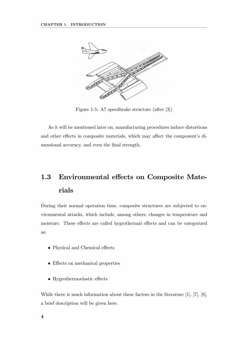
1-5 A7 speedbrake structure (after [3]) . . . . . . . . . . . . . . . . . 4
1-6 Unsymmetrical CFRP laminate . . . . . . . . . . . . . . . . . . . 6
2-1 Residual stress formation after cool down (after [4]) . . . . . . . . 9
2-2 Grooving experimental setup (after [5]) . . . . . . . . . . . . . . . 13
2-3 Main components of a typical drilling equipment for residual stress
analysis (after [6]) . . . . . . . . . . . . . . . . . . . . . . . . . . . 14
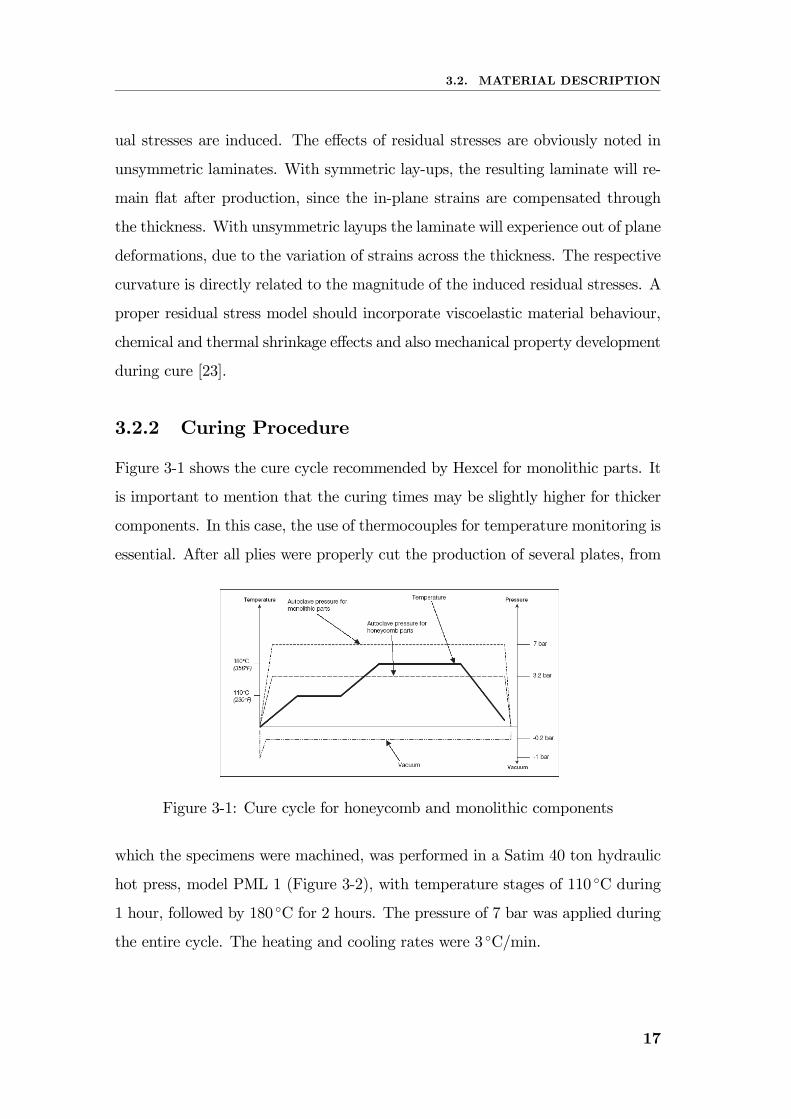
3-1 Cure cycle for honeycomb and monolithic components . . . . . . . 17
3-2 Satim hydraulic hot press . . . . . . . . . . . . . . . . . . . . . . 18
3-3 Stress-strain relation for the 0 specimens loaded in tension . . . 21
3-4 Stress-strain relation for the 90 specimens loaded in tension . . . 22
3-5 Stress-strain relation for the shear specimens loaded in tension . . 24
3-6 Plate and specimens’ dimensions (mm) . . . . . . . . . . . . . . . 26
3-7 Dilatometer . . . . . . . . . . . . . . . . . . . . . . . . . . . . . . 27
3-8 Heating and cooling rates . . . . . . . . . . . . . . . . . . . . . . 27
3-9 Results of the dilatometer test in the longitudinal direction . . . . 27
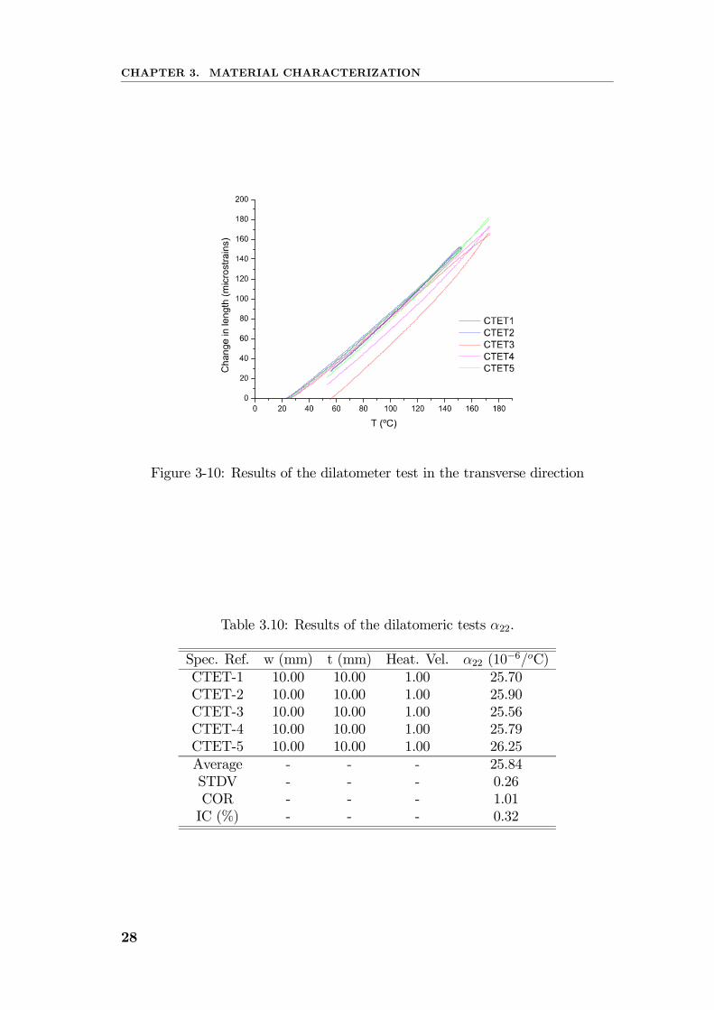
3-10 Results of the dilatometer test in the transverse direction . . . . . 28
3-11 Measured height . . . . . . . . . . . . . . . . . . . . . . . . . . . . 29
3-12 Determination of the stress free temperature . . . . . . . . . . . . 29
xiii
xiv LIST OF FIGURES
3-13 Flowchart for the stress free temperature . . . . . . . . . . . . . . 29
3-14 Laminate micrograph . . . . . . . . . . . . . . . . . . . . . . . . . 30
3-15 Flowchart for the determination of microscopic properties . . . . . 33
3-16 Ply designation . . . . . . . . . . . . . . . . . . . . . . . . . . . . 34
3-17 Autoclave equipment used . . . . . . . . . . . . . . . . . . . . . . 35
4-1 Reference plane and ply coordinates (after [1]) . . . . . . . . . . . 38
4-2 Classical Laminate Theory flowchart . . . . . . . . . . . . . . . . 41
5-1 Dimensions of the specimen used with the HDM . . . . . . . . . . 46
5-2 Parameters of the rosette strain gauge . . . . . . . . . . . . . . . 47
5-3 Specimen used for microscopic inspection . . . . . . . . . . . . . . 48
5-4 Cross ply laminate micrograph . . . . . . . . . . . . . . . . . . . . 49
5-5 Quasi isotropic laminate micrograph . . . . . . . . . . . . . . . . 49
5-6 Applied load to determine Ain . . . . . . . . . . . . . . . . . . . . 50
5-7 Nodes where the displacements are determined . . . . . . . . . . . 51
5-8 Applied load to determine Bin and Cin . . . . . . . . . . . . . . . 51
5-9 Fortran subroutine DLOAD . . . . . . . . . . . . . . . . . . . . . 52
5-10 Fourth drilling stage . . . . . . . . . . . . . . . . . . . . . . . . . 52
5-11 First increment . . . . . . . . . . . . . . . . . . . . . . . . . . . . 53
5-12 Second increment . . . . . . . . . . . . . . . . . . . . . . . . . . . 53
5-13 Third increment . . . . . . . . . . . . . . . . . . . . . . . . . . . . 53
5-14 Fourth increment . . . . . . . . . . . . . . . . . . . . . . . . . . . 54
5-15 Fifth increment . . . . . . . . . . . . . . . . . . . . . . . . . . . . 54
5-16 Sixth increment . . . . . . . . . . . . . . . . . . . . . . . . . . . . 55
5-17 Seventh increment . . . . . . . . . . . . . . . . . . . . . . . . . . 55
5-18 Eighth increment . . . . . . . . . . . . . . . . . . . . . . . . . . . 56
5-19 Displacements U1 (θn = 0) . . . . . . . . . . . . . . . . . . . . . . 56
5-20 Displacements U1 (θn = π2) . . . . . . . . . . . . . . . . . . . . . . 57
5-21 Displacements U1 (θn = π4) . . . . . . . . . . . . . . . . . . . . . . 57
5-22 Experimental setup used for the drilling procedure . . . . . . . . . 58
LIST OF FIGURES xv
5-23 Measured strains . . . . . . . . . . . . . . . . . . . . . . . . . . . 58
5-24 Longitudinal residual stresses after curing . . . . . . . . . . . . . 59
5-25 Transversal residual stresses after curing . . . . . . . . . . . . . . 59
5-26 Measured strains . . . . . . . . . . . . . . . . . . . . . . . . . . . 60
5-27 Longitudinal residual stresses one month after curing . . . . . . . 60
5-28 Transversal residual stresses one month after curing . . . . . . . . 61
5-29 Measured strains . . . . . . . . . . . . . . . . . . . . . . . . . . . 61
5-30 Longitudinal residual stresses two months after curing . . . . . . . 62
5-31 Transversal residual stresses two months after curing . . . . . . . 62
5-32 Evolution of residual stresses (σ1) for the 0o plies . . . . . . . . . 63
5-33 Evolution of residual stresses (σ2) for the 0o plies . . . . . . . . . 63
5-34 Evolution of residual stresses (σ1) for the 90o plies . . . . . . . . . 64
5-35 Evolution of residual stresses (σ2) for the 90o plies . . . . . . . . . 65
5-36 Schematic curves representing linear and non-linear absorption
processes . . . . . . . . . . . . . . . . . . . . . . . . . . . . . . . . 67
5-37 Geometry of specimens used for absorption experiments . . . . . . 68
5-38 Weighing device for the determination of absorbed moisture . . . 68
5-39 Moisture absorption possibilities . . . . . . . . . . . . . . . . . . . 69
5-40 Illustration of the change of moisture content with the square root
of time. For t<tL the slope is constant . . . . . . . . . . . . . . . 71
5-41 Moisture absorption for the [0/90] laminates . . . . . . . . . . . . 72
5-42 Moisture absorption for the [0/902] laminates . . . . . . . . . . . 73
5-43 Moisture absorption for the [0/904] laminates . . . . . . . . . . . 73
5-44 Moisture absorption for the [90/0/903] laminates . . . . . . . . . . 74
5-45 Curvature evolution with moisture . . . . . . . . . . . . . . . . . 74
5-46 Curvature evolution with immersion time . . . . . . . . . . . . . . 75
6-1 Geometry and boundary conditions used . . . . . . . . . . . . . . 77
6-2 Stress distribution with hole . . . . . . . . . . . . . . . . . . . . . 78
6-3 Stress distribution with removed elements . . . . . . . . . . . . . 78
6-4 Stress distribution along the hole boundary . . . . . . . . . . . . . 79
xvi LIST OF FIGURES
6-5 Out of plane displacements of the [0/90] laminate . . . . . . . . . 80
6-6 Out of plane displacements of the [0/902] laminate . . . . . . . . . 80
6-7 Out of plane displacements of the [0/904] laminate . . . . . . . . . 81
6-8 Out of plane displacements of the [90/0/903] laminate . . . . . . . 81
6-9 Laminate curvature calculation . . . . . . . . . . . . . . . . . . . 82
6-10 Square cell arrangement . . . . . . . . . . . . . . . . . . . . . . . 83
6-11 σVM/σyd (Vf = 30%) . . . . . . . . . . . . . . . . . . . . . . . . . 84
6-12 σVM/σyd (Vf = 60%) . . . . . . . . . . . . . . . . . . . . . . . . . 85
6-13 σVM/σyd (Vf = 78.5%) . . . . . . . . . . . . . . . . . . . . . . . . 86
6-14 σVM/σyd distribution in the matrix . . . . . . . . . . . . . . . . . 87
6-15 Energy based damage criterion (Vf = 30%) . . . . . . . . . . . . . 88
6-16 Energy based damage criterion (Vf = 60%) . . . . . . . . . . . . . 89
6-17 Energy based damage criterion (Vf = 78.5%) . . . . . . . . . . . . 89
6-18 UV /UcrV distribution of the square unit cell at the fibre-matrix border 90
6-19 Hexagonal cell arrangement . . . . . . . . . . . . . . . . . . . . . 90
6-20 σVM/σyd (Vf = 30%) . . . . . . . . . . . . . . . . . . . . . . . . . 91
6-21 σVM/σyd distribution (Vf = 60%) . . . . . . . . . . . . . . . . . . 91
6-22 σVM/σyd distribution (Vf = 90%) . . . . . . . . . . . . . . . . . . 92
6-23 σVM/σyd distribution in the matrix for the bottom fibre . . . . . . 92
6-24 σVM/σyd distribution in the matrix for the top fibre . . . . . . . . 93
6-25 Energy based damage criterion (Vf = 30%) . . . . . . . . . . . . . 93
6-26 Energy based damage criterion (Vf = 60%) . . . . . . . . . . . . . 94
6-27 Energy based damage criterion (Vf = 90%) . . . . . . . . . . . . . 94
6-28 Uv/Ucr distribution in the matrix for the bottom fibre . . . . . . . 95
6-29 Uv/Ucr distribution in the matrix for the top fibre . . . . . . . . . 95
List of Tables
3.1 Longitudinal tensile test matrix . . . . . . . . . . . . . . . . . . . 20
3.2 Results of the longitudinal tensile test- specimens with tapered end
tabs. . . . . . . . . . . . . . . . . . . . . . . . . . . . . . . . . . . 21
3.3 Transversal tensile test matrix . . . . . . . . . . . . . . . . . . . . 22
3.4 Results of the transverse tensile test. . . . . . . . . . . . . . . . . 23
3.5 Shear test matrix . . . . . . . . . . . . . . . . . . . . . . . . . . . 23
3.6 Results of the shear tests. . . . . . . . . . . . . . . . . . . . . . . 24
3.7 Ply properties (transversely isotropic) . . . . . . . . . . . . . . . . 24
3.8 Measured parameters . . . . . . . . . . . . . . . . . . . . . . . . . 25
3.9 Results of the dilatomeric tests α11 . . . . . . . . . . . . . . . . . 25
3.10 Results of the dilatomeric tests α22. . . . . . . . . . . . . . . . . . 28
3.11 Fibre and matrix moduli . . . . . . . . . . . . . . . . . . . . . . . 32
3.12 Coefficients of thermal expansion . . . . . . . . . . . . . . . . . . 32
3.13 Specimen characterisitcs for the hole drilling experiments . . . . . 33
3.14 Specimen characterisitcs for the moisture absorption experiments 34
5.1 Test plan for the hole drilling method . . . . . . . . . . . . . . . . 46
5.2 Strain gauge caracteristics . . . . . . . . . . . . . . . . . . . . . . 47
5.3 Calibration coefficients . . . . . . . . . . . . . . . . . . . . . . . . 57
5.4 Hole drilling parameters . . . . . . . . . . . . . . . . . . . . . . . 58
5.5 Test plan for the moisture absorption experiments . . . . . . . . . 67
5.6 Weight comparison after drying . . . . . . . . . . . . . . . . . . . 71
6.1 Comparison of curvatures (experimental and CLT) . . . . . . . . 82
xvii

xviii LIST OF TABLES
6.2 Comparison of curvatures (experimental and FEM) . . . . . . . . 83

List of Symbols
εin Radial strain in layer i at increment n
σxx Normal stress along x axis
σyy Normal stress along y axis
σ11 Normal ply stress along fibre direction
σ22 Normal ply stress perpendicular to fibre direction
σVM Von Mises stress
σyd Yielding stress
XLT Unnotched laminate tensile strength
XT Ply longitudinal tensile strength
XC Ply longitudinal compressive strength
YT Ply transverse tensile strength
YC Ply transverse compressive strength
SL Tensile shear strength in the longitudinal direction
ST Tensile shear strength in the transverse direction
GIc Mode I fracture toughness for transverse crack propagation
Y isT In-situ ply transverse tensile strength
κ Curvature
UV Dilatational energy density
Ucr Critical dilatational energy density
xix

xx LIST OF TABLES
θi Angle between principal stress directions and global system
υ12 Major Poisson’s ratio
E1 Longitudinal modulus of elasticity
E2 Transverse modulus of elasticity
G12 In-plane shear modulus
t Thickness
Em Matrix modulus
Ef Fibre modulus
t∗ Non-dimensional time
d Hole diameter
w Width
α11 Coefficient of thermal expansion in the longitudinal direction
α22 Coefficient of thermal expansion in the transversal direction
Vf Fibre volume fraction
M Moisture content
G Time dependent parameter
Dx Diffusivity

List of Abbreviations
ASTM American Society for Testing and Materials
CLT Classical Lamination Theory
CFRP Carbon Fibre Reinforced Plastics
CTE Coefficient of thermal expansion
FEM Finite elements model
FW Filament winding
HDM Hole drilling method
OHT Open-hole tensile
PMC Polymer matrix composite
RS Residual stress
RTM Resin Transfer Molding
SFT Stress free temperature
TTS Transverse tensile strength
xxi

xxii
Acknowledgements
This work would not have been possible without the precious help of the following
individuals and institutions:
Dr. Pedro Ponces Camanho, INEGI, (CEFAD)
Dr. António Torres Marques, INEGI, (CEMACOM)
Dr. João Paulo Nobre, FCTUC
Dra. Maria Teresa Restivo, FEUP
Célia Novo (MSc, INEGI, (CEMACOM)
Eng. Joaquim Fonseca, FEUP
Mr. José and Mr. Albino, FEUP
Mrs. Emilia Soares, FEUP
I would also like to thank for all support:
Cassilda Tavares (MSc, PhD student), IDMEC
Pedro Portela, Pedro Bandeira (MSc students), INEGI, (CEFAD)
Raul Campilho (MSc student)
For all software and hardware problems solutions, I am deeply thankful to:
Pedro Martins (PhD student), IDMEC
Marco Parente (PhD student)
Also, I shall not forget all of those who contribute to a healthy and charming
workspace environment:
David Perez (PhD student)
Jorge Belinha (MSc student)
Paulo Neves (FCT colaborator)
Carla Roque (PhD student)
xxiii
Chapter 1
Introduction
1.1 Basic Definitions
Many structural applications require the use of materials combining, simultane-
ously, superior strength and stiffness with low weight. Composite materials are
excellent candidates for fulfilling these requirements because of their high specific
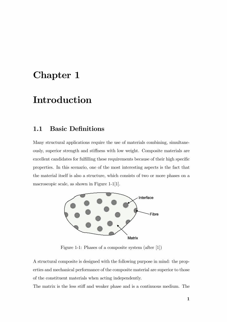
properties. In this scenario, one of the most interesting aspects is the fact that
the material itself is also a structure, which consists of two or more phases on a
macroscopic scale, as shown in Figure 1-1[1].
Figure 1-1: Phases of a composite system (after [1])
A structural composite is designed with the following purpose in mind: the prop-
erties and mechanical performance of the composite material are superior to those
of the constituent materials when acting independently.
The matrix is the less stiff and weaker phase and is a continuous medium. The
1
CHAPTER 1. INTRODUCTION
reinforcement is usually discontinuous, stiffer and stronger. Needless to say, the
properties of a composite structure depend on the properties of the constituents,
geometry and phase distribution. The homogeneity of the material system de-
pends on the more or less distribution of the reinforcement. Composite materials
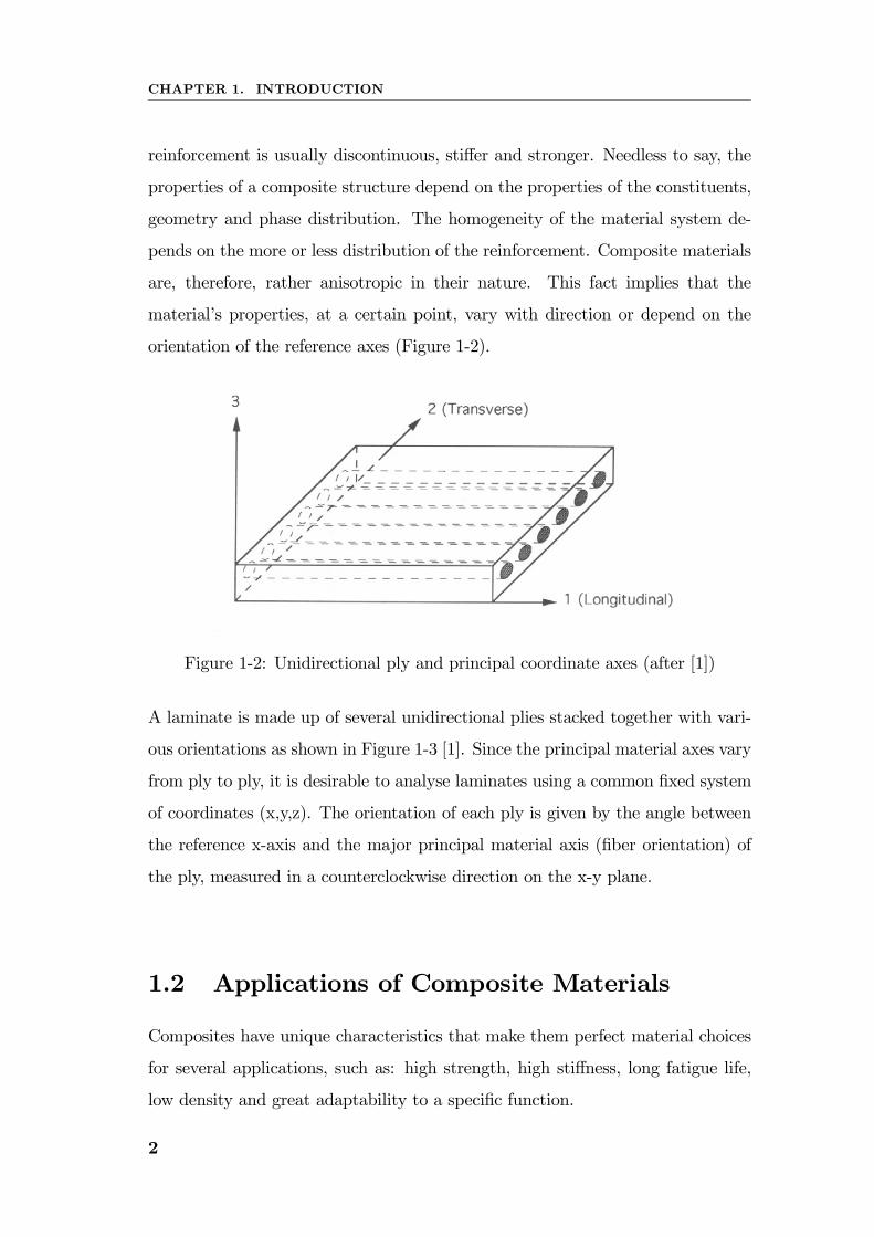
are, therefore, rather anisotropic in their nature. This fact implies that the
material’s properties, at a certain point, vary with direction or depend on the
orientation of the reference axes (Figure 1-2).
Figure 1-2: Unidirectional ply and principal coordinate axes (after [1])
A laminate is made up of several unidirectional plies stacked together with vari-
ous orientations as shown in Figure 1-3 [1]. Since the principal material axes vary
from ply to ply, it is desirable to analyse laminates using a common fixed system
of coordinates (x,y,z). The orientation of each ply is given by the angle between
the reference x-axis and the major principal material axis (fiber orientation) of
the ply, measured in a counterclockwise direction on the x-y plane.
1.2 Applications of Composite Materials
Composites have unique characteristics that make them perfect material choices
for several applications, such as: high strength, high stiffness, long fatigue life,
low density and great adaptability to a specific function.
2
1.2. APPLICATIONS OF COMPOSITE MATERIALS
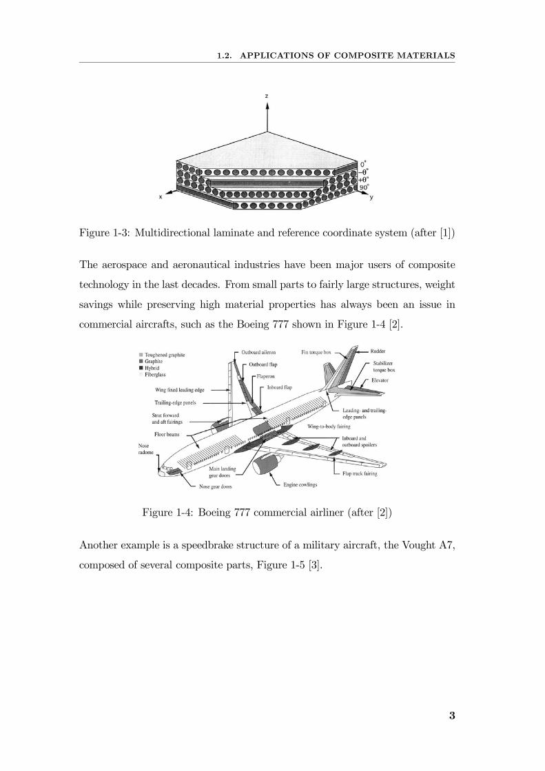
Figure 1-3: Multidirectional laminate and reference coordinate system (after [1])
The aerospace and aeronautical industries have been major users of composite
technology in the last decades. From small parts to fairly large structures, weight
savings while preserving high material properties has always been an issue in
commercial aircrafts, such as the Boeing 777 shown in Figure 1-4 [2].
Figure 1-4: Boeing 777 commercial airliner (after [2])
Another example is a speedbrake structure of a military aircraft, the Vought A7,
composed of several composite parts, Figure 1-5 [3].
3
CHAPTER 1. INTRODUCTION
Figure 1-5: A7 speedbrake structure (after [3])
As it will be mentioned later on, manufacturing procedures induce distortions
and other effects in composite materials, which may affect the component’s di-
mensional accuracy, and even the final strength.
1.3 Environmental effects on Composite Mate-
rials
During their normal operation time, composite structures are subjected to en-
vironmental attacks, which include, among others, changes in temperature and
moisture. These effects are called hygrothermal effects and can be categorized
as:
• Physical and Chemical effects
• Effects on mechanical properties
• Hygrothermoelastic effects
While there is much information about these factors in the literature [1], [7], [8],
a brief description will be given here.
4
1.4. SCOPE OF THIS WORK
1.3.1 Physical and Chemical effects
Moisture absorption and desorption processes in polymer matrix composites de-
pend on the current hygrothermal state and on the environment. Basically the
moisture content in the material affects the glass transition temperature of the
matrix. Polymerization processes are a function of the hygrothermal properties
of the constituents and the composite’s current hygrothermal state. Material
degradation and corrosion can also be related to hygrothermal factors.
1.3.2 Effects on mechanical properties
Time dependent properties such as the tensile modulus and shear modulus may
vary with temperature and moisture concentration. Failure and strenght charac-
teristics, specially interfacial and matrix dominated ones, may depend on tem-
perature and humidity.
1.3.3 Hygrothermoelastic effects
The composite material undergoes reversible deformations related to thermal
expansion (α) and moisture expansion (β) coefficients. Intralaminar and inter-
laminar stresses are developed as a result of the thermoelastic and hygroelastic
inhomogeneity and anisotropy of the material.
1.4 Scope of this work
Basically, the starting point for this work is the following open question: how
is the evolution of the residual thermal stresses in composites as a function of
time and environmental conditions. In order to further investigate this question
the discussion is organized as follows: first, a literature survey is presented. In
chapter 3 the material characterization process is discussed in detail. The exper-
imental procedures and the respective results are presented in chapter 5. Some
analytical and numerical models were developed and the respective results are
5
CHAPTER 1. INTRODUCTION
discussed in chapter 6. In chapter 7, the final conclusions and suggestions for fu-
ture developments are presented. In this work, symmetrical and unsymmetrical
laminates will be analysed. The residual stress level after curing and the possible
stress relaxation were investigated for both laminates. For the symmetrical lami-
nates the hole drilling method (HDM) was used to determine the state of residual
stress. Although the HDM has been used to quantify the level of residual stresses
in composites subjected to various cooling conditions, no report regarding it’s
application to study the experimental evolution of residual stresses with time
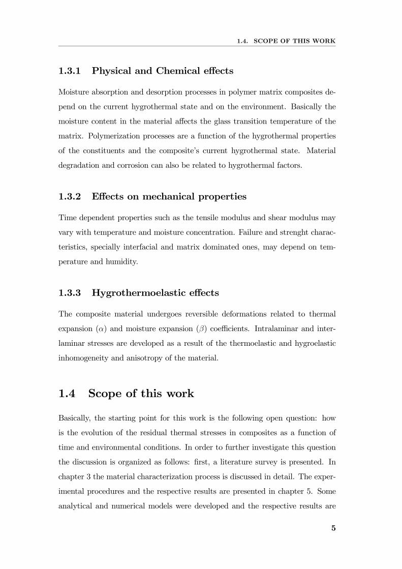
was available at the time of this work. The study regarding unsymmetrical lami-
nates like the one shown in Figure 1-6 relied mostly on the measurement of their
curvature. The moisture effect was also investigated. Unsymmetrical specimens
Figure 1-6: Unsymmetrical CFRP laminate
with various stacking sequences were immersed in water and the weight gain was
related to their curvature change. The curvature of the laminates were also pre-
dicted using analytical and numerical tools. The results were then compared with
experimental data. It is also a goal of this work to provide experimental data in
all possible domains for the IM7/8552 prepreg. This material is widely used in
the aeronautical and aerospace industries.
6
Chapter 2
Residual Stresses in Composite
Materials
2.1 Development of residual stresses
One may define residual stresses in composite laminates as locked-in stresses
without application of any exterior forces. This is the most basic definition that
may be found in the literature.
In the case of multidirectional laminates, residual stresses are introduced during
the fabrication process, and the understanding of the effects of residual stresses
on the material response is needed [1], [4]. After curing and cooling the com-
posite, the matrix is subject to a tri-axial stress state. Shrinkage during curing
and the mismatch of coefficients of thermal expansion between fibre and matrix
are the most important reasons for residual stresses. Since the fibre’s coefficient
of thermal expansion is lower compared to the matrix coefficient of thermal ex-
pansion, the resulting thermal residual stresses are of compressive nature in the
fibre and tensile nature in the matrix [9]. Residual stresses may be analysed from
a micromechanical or macromechanical point of view. On the micromechanical
scale, residual stresses appear in unidirectional layers in and around individual
fibres due to the mismatch in thermal properties of the constituents, like the
difference in coefficients of thermal expansion. On a macroscopic level, laminate
7
CHAPTER 2. RESIDUAL STRESSES IN COMPOSITE MATERIALS
residual stresses develop due to the thermal anisotropy of the respective layers.
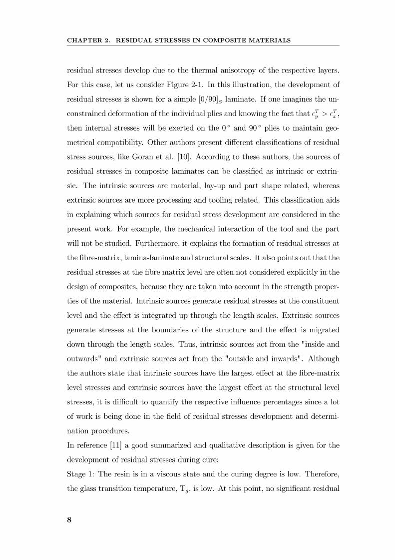
For this case, let us consider Figure 2-1. In this illustration, the development of
residual stresses is shown for a simple [0/90]S laminate. If one imagines the un-
constrained deformation of the individual plies and knowing the fact that Ty > T
x ,
then internal stresses will be exerted on the 0 and 90 plies to maintain geo-
metrical compatibility. Other authors present different classifications of residual
stress sources, like Goran et al. [10]. According to these authors, the sources of
residual stresses in composite laminates can be classified as intrinsic or extrin-
sic. The intrinsic sources are material, lay-up and part shape related, whereas
extrinsic sources are more processing and tooling related. This classification aids
in explaining which sources for residual stress development are considered in the
present work. For example, the mechanical interaction of the tool and the part
will not be studied. Furthermore, it explains the formation of residual stresses at
the fibre-matrix, lamina-laminate and structural scales. It also points out that the
residual stresses at the fibre matrix level are often not considered explicitly in the
design of composites, because they are taken into account in the strength proper-
ties of the material. Intrinsic sources generate residual stresses at the constituent
level and the effect is integrated up through the length scales. Extrinsic sources
generate stresses at the boundaries of the structure and the effect is migrated
down through the length scales. Thus, intrinsic sources act from the "inside and
outwards" and extrinsic sources act from the "outside and inwards". Although
the authors state that intrinsic sources have the largest effect at the fibre-matrix
level stresses and extrinsic sources have the largest effect at the structural level
stresses, it is difficult to quantify the respective influence percentages since a lot
of work is being done in the field of residual stresses development and determi-
nation procedures.
In reference [11] a good summarized and qualitative description is given for the
development of residual stresses during cure:
Stage 1: The resin is in a viscous state and the curing degree is low. Therefore,
the glass transition temperature, Tg, is low. At this point, no significant residual
8
2.2. RESIDUAL STRESS EFFECTS
stresses occur.
Stage 2: This stage starts at the gel point of the resin. For epoxy resins, this
happens for a degree of cure of about 0.6. Degree of cure represents the extent
to which curing of a thermosetting resin has progressed. From this point, the
resin modulus begins to grow and the material picks up some stresses, which
are quickly relieved because the temperature is relatively high comparing to Tg,
being the material highly viscoelastic.
Stage 3: The start of the resin’s vitrification is the point at which Tg coincides
with the cure temperature. From this point on until cool down to room temper-
ature the stresses developed contribute greatly to the total amount of residual
stress of the material.
Figure 2-1: Residual stress formation after cool down (after [4])
2.2 Residual stress effects
Lu et al. [12] investigated the influence of residual stresses due mainly to fab-
rication conditions on the mechanical behaviour of composite laminates. The
9
CHAPTER 2. RESIDUAL STRESSES IN COMPOSITE MATERIALS
authors used CFRP laminates that were processed from unidirectional T300/914
prepeg. A cross-ply structure was used, with the following orientation and stack-
ing sequence: [02/902]S. Three different cooling conditions were applied after the
material’s curing cycle, namely fast, normal and slow. The residual stress distri-
bution along the laminate’s thickness was experimentally determined using the
hole drilling method, and also numerically, through the finite element method.
Tensile tests were performed on the cured specimens. Lu et al. [12] concluded
that the presence of a residual stress field does not influence the initial stiffness of
the laminate. Differences between the ultimate tensile stresses corresponding to
the three cooling conditions were observed. Stringer et al. [13] investigated the
formation of residual stresses in thick polymer composites. In this case, the com-
ponent was too rigid for residual stresses to be relieved by deformation ( zz = 0).
The existence of a tri-axial stress state is more favourable to the occurrence of
internal damage such as delamination cracking. Stringer et al. [13] used embed-
ded electrical resistance strain gauges and optic fibre strain sensors to monitor
residual stresses during manufacturing. The processes studied were resin transfer
molding (RTM) and filament winding (FW). The model developed by Stinger
et al. suggested in the case of FW that a heated mandrel significantly reduces
residual stresses. A lot of chemistry is involved in the online monitoring of resid-
ual stress fields. Therefore a fairly developed cure kinetics model is needed if
one wishes to determine the residual stresses at any time during the cure cycle.
Stringer et al. [13] pointed out an important fact related to the time at which
residual stresses begin to build up: before gelation time no significant physical
union exists between the matrix resin and reinforcing material, the fibres. At
gelation time, the resin solidifies and it is at this point that meaningful internal
residual strains begin to appear. This is important, since most residual stress
predictions are determined using Tg as the maximum cure reference temperature.
Residual stresses (RS) in composite laminates depend on thermoelastic prop-
erties of the material and processing temperature. The RS distribution in the
various laminae depends on the stacking sequence and ply orientation. Resid-
10
2.3. EXPERIMENTAL METHODS FOR ASSESSING RESIDUAL STRESSES IN
COMPOSITE MATERIALS
ual stresses may have undesirable effects on the material: distortions of finished
components when cooled and removed from moulds, creating dimensional insta-
bility and locked-in stresses, which may cause delamination cracking. Tensile
residual stresses in the matrix are particularly important because they may rep-
resent a significant fraction of the tensile strength of the polymer and can lead to
premature failure by matrix cracking. Nairn points out that the residual stress
effects should be included in every composite fracture model because they may
contribute to the energy release rate [14].
2.3 Experimental Methods for assessing resid-
ual stresses in composite materials
Many experimental techniques are described in the literature for the determi-
nation of residual stresses in composite materials. It is important to mention
the main advantages and disadvantages of each one. A brief description of each
technique will be given in the following subsections. One thing to remind is that
residual stresses cannot be measured directly: the residual strains must be first
determined and then proceed to calculate the stresses.
2.3.1 Embedded Strain Gauges
The use of embedded strain gauges in composite laminates to directly measure
process induced strains is quite expensive because it requires special strain gauges
capable of supporting high curing temperatures and pressures [15]. Also, it is not
very practical, since a precise alignment of the strain gauges is needed and it may
be quite difficult to achieve. Further, it creates a localised delamination in the
composite material, whose effect on the measured strains is unknown.
11
CHAPTER 2. RESIDUAL STRESSES IN COMPOSITE MATERIALS
2.3.2 X-Ray Diffraction
In reference [16] a X-Ray diffraction method for determining thermal residual
stresses in unidirectional laminates is proposed. The authors use embedded alu-
minum and silver inclusions placed between certain plies of a laminate. The
experimental results are then compared with numerical results. The main advan-
tage of this method is that it allows to obtain the complete stress tensor. In the
specimens investigated in this work [16], a triaxial state of stress exists, which
would not be detected if another process relying on plane stress state was used.
On the other hand, this method has some drawbacks, which are related to the fact
that particle shape has a strong influence on the measured X-Ray stresses. Also,
for the method to be more accurate, the particles’ distribution in the laminate
needs to be strictly controlled. This method is clearly not suitable for measuring
residual stresses in previously manufactured structures.
2.3.3 Successive Grooving Technique
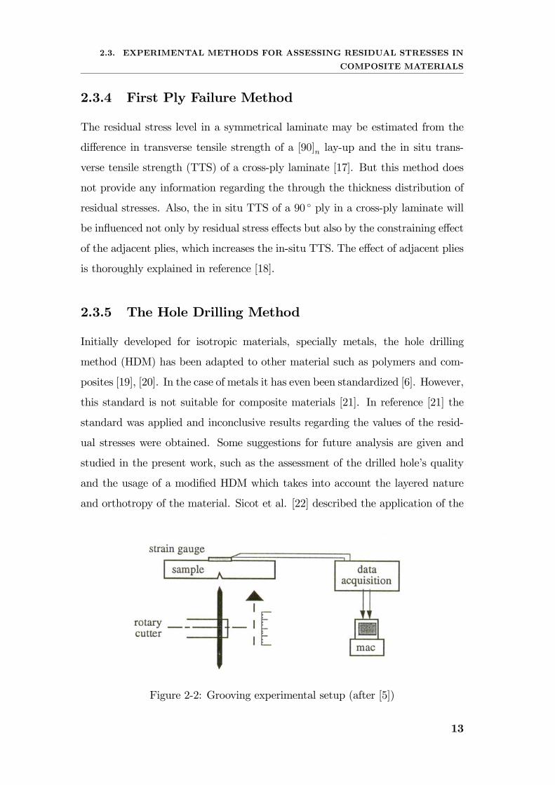
Yu et al. [5] describe a technique involving the cut of a progressively deepening
thin slit through the thickness of a composite part promoting stress relaxation.
For strain measuring, a strain gauge must be placed on the face of the part
opposite to the groove, as shown in Figure 2-2. Cutting the groove modifies
the overall stress field within the part, and its geometry changes until another
self-equilibrating state of stress is attained. The internal through the thickness
residual stresses may then be determined. Although the authors mention the key
advantage of this method being the low quantity of removed material, the precise
alignment of the cutting element and the strain gauge is difficult to achieve. Also,
the location of the strain sensing device may not be achievable for larger parts
or structures.
12
2.3. EXPERIMENTAL METHODS FOR ASSESSING RESIDUAL STRESSES IN
COMPOSITE MATERIALS
2.3.4 First Ply Failure Method
The residual stress level in a symmetrical laminate may be estimated from the
difference in transverse tensile strength of a [90]n lay-up and the in situ trans-
verse tensile strength (TTS) of a cross-ply laminate [17]. But this method does
not provide any information regarding the through the thickness distribution of
residual stresses. Also, the in situ TTS of a 90 ply in a cross-ply laminate will
be influenced not only by residual stress effects but also by the constraining effect
of the adjacent plies, which increases the in-situ TTS. The effect of adjacent plies
is thoroughly explained in reference [18].
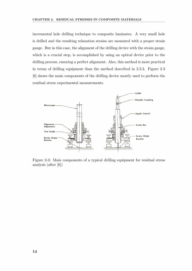
2.3.5 The Hole Drilling Method
Initially developed for isotropic materials, specially metals, the hole drilling
method (HDM) has been adapted to other material such as polymers and com-
posites [19], [20]. In the case of metals it has even been standardized [6]. However,
this standard is not suitable for composite materials [21]. In reference [21] the
standard was applied and inconclusive results regarding the values of the resid-
ual stresses were obtained. Some suggestions for future analysis are given and
studied in the present work, such as the assessment of the drilled hole’s quality
and the usage of a modified HDM which takes into account the layered nature
and orthotropy of the material. Sicot et al. [22] described the application of the
Figure 2-2: Grooving experimental setup (after [5])
13
CHAPTER 2. RESIDUAL STRESSES IN COMPOSITE MATERIALS
incremental hole drilling technique to composite laminates. A very small hole
is drilled and the resulting relaxation strains are measured with a proper strain
gauge. But in this case, the alignment of the drilling device with the strain gauge,
which is a crucial step, is accomplished by using an optical device prior to the
drilling process, ensuring a perfect alignment. Also, this method is more practical
in terms of drilling equipment than the method described in 2.3.3. Figure 2-3
[6] shows the main components of the drilling device mostly used to perform the
residual stress experimental measurements.
Figure 2-3: Main components of a typical drilling equipment for residual stressanalysis (after [6])
14
Chapter 3
Material Characterization
3.1 Introduction
The determination of the mechanical properties relevant to this work is of cru-
cial importance. The mechanical properties are inputs for the numerical and
analytical procedures. Mechanical as well as thermomechanical properties were
determined following standard procedures. Although some of the properties are
available from the material’s manufacturer, it is always advisable to conduct ex-
periments to determine the material’s properties, since deviations may occur. In
this Chapter a brief description of all test procedures is given.
3.2 Material Description
For the manufacture of all specimens a Hexcel’s IM7/8552 carbon epoxy unidi-
rectional pre-preg was chosen. It is a high performance composite material used
mostly in the aeronautical and aerospace industries. The material was properly
conditioned, according to the manufacturer’s instructions.
3.2.1 Curing cycle and Residual Stress Development
In the production of composite parts the pertinent processing parameters are
time, temperature and pressure. Slight deviations from the recommended pro-
15
CHAPTER 3. MATERIAL CHARACTERIZATION
cessing conditions can result in unacceptable quality. One of the most signifi-
cant problems in the processing of composites is residual stresses, as processing-
induced residual stresses can be high enough to cause cracking within the matrix
even before mechanical loading. This microcracking of the matrix can expose the
fibers to degradation by chemical attack. Strength is adversely affected by resid-
ual stresses since a pre-loading has been introduced. White et al. [23] describe a
model which predicts the residual stress history during cure. Since this work is
focused only on the final stress state after curing, the models will be considered
linear elastic, i.e. the analysis is restricted to the cooldown phase of the cure cy-
cle. Nevertheless, a detailed description of the curing cycle will be given to allow
for a better understanding of the formation of residual stresses. The standard
process cycle for polymer matrix composites (PMCs) is a two step cure cycle. In
such cycles the temperature of the material is increased from room temperature
to the first dwell temperature and this temperature is held constant for about
one hour. Afterwards, the temperature is increased again to the second dwell
temperature and held constant for two to eigth hours. Then, the part is cooled
down to room temperature at a constant rate. The purpose of the first dwell is to
allow gases (entrapped air, water or volatiles) to escape the matrix material and
to allow the matrix to flow, thus facilitating compaction of the part. This means
the viscosity must be low during the first dwell. The purpose of the second dwell
is to allow crosslinking of the polymer to take place. It is in this phase that the
strength and related mechanical properties of the composite are developed. The
issue of residual stresses becomes more important when high-temperature resins
are involved, because they are processed at higher temperatures. Chemically, the
reinforcing fibres are affected very little during the process cycle. The polymer
matrix on the other hand will contract during crosslinking by as much as 6% in
thermosets. Regarding thermally-induced deformations, these occur because the
polymer matrix has a higher CTE than the fibre, typically an order of magnitude
or more. After processing, the composite must be well-bonded and continuous,
so these deformations are balanced internally within the composite and resid-
16
3.2. MATERIAL DESCRIPTION
ual stresses are induced. The effects of residual stresses are obviously noted in
unsymmetric laminates. With symmetric lay-ups, the resulting laminate will re-
main flat after production, since the in-plane strains are compensated through
the thickness. With unsymmetric layups the laminate will experience out of plane
deformations, due to the variation of strains across the thickness. The respective
curvature is directly related to the magnitude of the induced residual stresses. A
proper residual stress model should incorporate viscoelastic material behaviour,
chemical and thermal shrinkage effects and also mechanical property development
during cure [23].
3.2.2 Curing Procedure
Figure 3-1 shows the cure cycle recommended by Hexcel for monolithic parts. It
is important to mention that the curing times may be slightly higher for thicker
components. In this case, the use of thermocouples for temperature monitoring is
essential. After all plies were properly cut the production of several plates, from
Figure 3-1: Cure cycle for honeycomb and monolithic components
which the specimens were machined, was performed in a Satim 40 ton hydraulic
hot press, model PML 1 (Figure 3-2), with temperature stages of 110 C during
1 hour, followed by 180 C for 2 hours. The pressure of 7 bar was applied during
the entire cycle. The heating and cooling rates were 3 C/min.
17
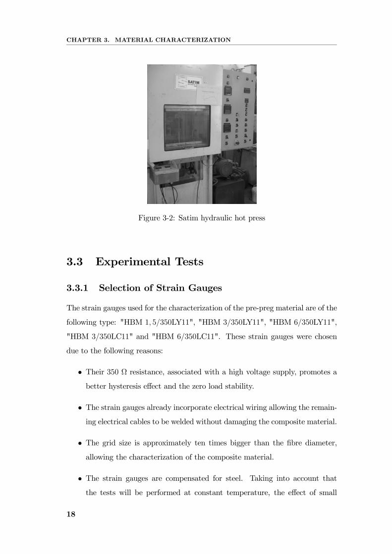
CHAPTER 3. MATERIAL CHARACTERIZATION
Figure 3-2: Satim hydraulic hot press
3.3 Experimental Tests
3.3.1 Selection of Strain Gauges
The strain gauges used for the characterization of the pre-preg material are of the
following type: "HBM 1, 5/350LY11", "HBM 3/350LY11", "HBM 6/350LY11",
"HBM 3/350LC11" and "HBM 6/350LC11". These strain gauges were chosen
due to the following reasons:
• Their 350 Ω resistance, associated with a high voltage supply, promotes a
better hysteresis effect and the zero load stability.
• The strain gauges already incorporate electrical wiring allowing the remain-
ing electrical cables to be welded without damaging the composite material.
• The grid size is approximately ten times bigger than the fibre diameter,
allowing the characterization of the composite material.
• The strain gauges are compensated for steel. Taking into account that
the tests will be performed at constant temperature, the effect of small
18
3.4. STRAIN GAUGE BONDING
temperature variations will be neglected.
• The strain gauges from series "C" are specially suited for the tests at tem-
perature extremes.
• The purchase cost was also a factor in their selection process.
The strain gauges were connected to the data acquisition system in quarter-bridge
using the three wires technique. This technique allows the system to be calibrated
so that temperature variations do not affect the measured data.
3.3.2 Surface preparation
Surface preparation is of crucial importance in strain gauging, because it influ-
ences the quality of the adhesion between the test specimen and the strain gauge.
The surface preparation will be performed as follows:
• Surface degreasing using "HBM - RMS1" cleaning solution, which is basi-
cally a mixture of acetone and isopropanol.
• Manually abrasion of the specimen surface with sandpaper n o 400.
• Cleaning with ethanol to remove the dust originated by the abrasion pro-
cess.
• Degreasing using "HBM - RMS1" to assure a total removal of all the possible
dust and grease that may remain on the specimen surface.
3.4 Strain gauge bonding
After the cleaning process, and to complete the strain gauging process, it is
necessary to execute the steps described beneath:
• Orientation guidelines are drawn upon the specimen surface to aid the cor-
rect alignment of the strain gauge.
19
CHAPTER 3. MATERIAL CHARACTERIZATION
• The strain gauge is finally glued using "HBM Z70", which is an acrylic
based adhesive.
The specimen is ready to be soldered to the data acquisition system wires. After
this process, the specimens were stored in an environmental chamber at 23 C
and 50% of relative humidity.
3.4.1 Ply Properties
Longitudinal Tensile Test
The purpose of the tensile tests is to measure the mechanical properties of the
ply under tensile loading. The tests were performed according to the ASTM [24]
test standard.The longitudinal tensile test measures the modulus of elasticity E1
and the major Poisson’s ratio ν12. Information regarding the lay-up and test
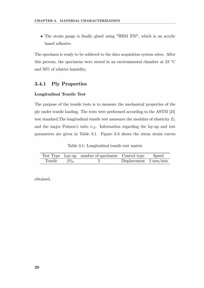
parameters are given in Table 3.1. Figure 3-3 shows the stress strain curves
Table 3.1: Longitudinal tensile test matrix
Test Type Lay-up number of specimens Control type SpeedTensile (0)8 5 Displacement 2 mm/min
obtained.
20
3.4. STRAIN GAUGE BONDING
Figure 3-3: Stress-strain relation for the 0 specimens loaded in tension
Table 3.2 shows the experimentally obtained values for E1, ν12 and XT .
Table 3.2: Results of the longitudinal tensile test- specimens with tapered endtabs.
Spec. Ref. w (mm) t (mm) E1 (GPa) υ12 XT (MPa)PT01C 15.01 0.98 138.84 0.31 2426.95PT02C 15.00 0.98 169.83 0.33 2298.23PT03C 15.00 0.98 170.57 0.29 2283.27PT04C 15.00 0.99 174.17 0.34 2308.42PT05C 15.00 0.99 173.68 0.31 2131.18Average 15.00 0.98 171.42 0.32 2289.61STDV - - 2.38 0.02 105.39COR - - 1.39 6.18 4.60IC (%) - - ± 2.95 ± 0.02 ± 130.84
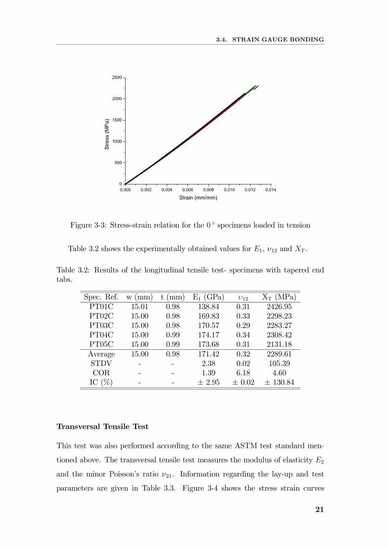
Transversal Tensile Test
This test was also performed according to the same ASTM test standard men-
tioned above. The transversal tensile test measures the modulus of elasticity E2
and the minor Poisson’s ratio ν21. Information regarding the lay-up and test
parameters are given in Table 3.3. Figure 3-4 shows the stress strain curves
21
CHAPTER 3. MATERIAL CHARACTERIZATION
Table 3.3: Transversal tensile test matrix
Test Type Lay-up number of specimens Control type SpeedTensile (90)16 5 Displacement 1 mm/min
obtained. Table 3.4 shows the results obtained in the 90o tensile tests.
σ
ε
Figure 3-4: Stress-strain relation for the 90 specimens loaded in tension
Shear Test
The shear tests were performed according to ASTM [25] to obtain the in-plane
shear modulus G12 and the in-plane shear strength SL. Information regarding
the lay-up and test parameters are given in Table 3.5. The results of the tests
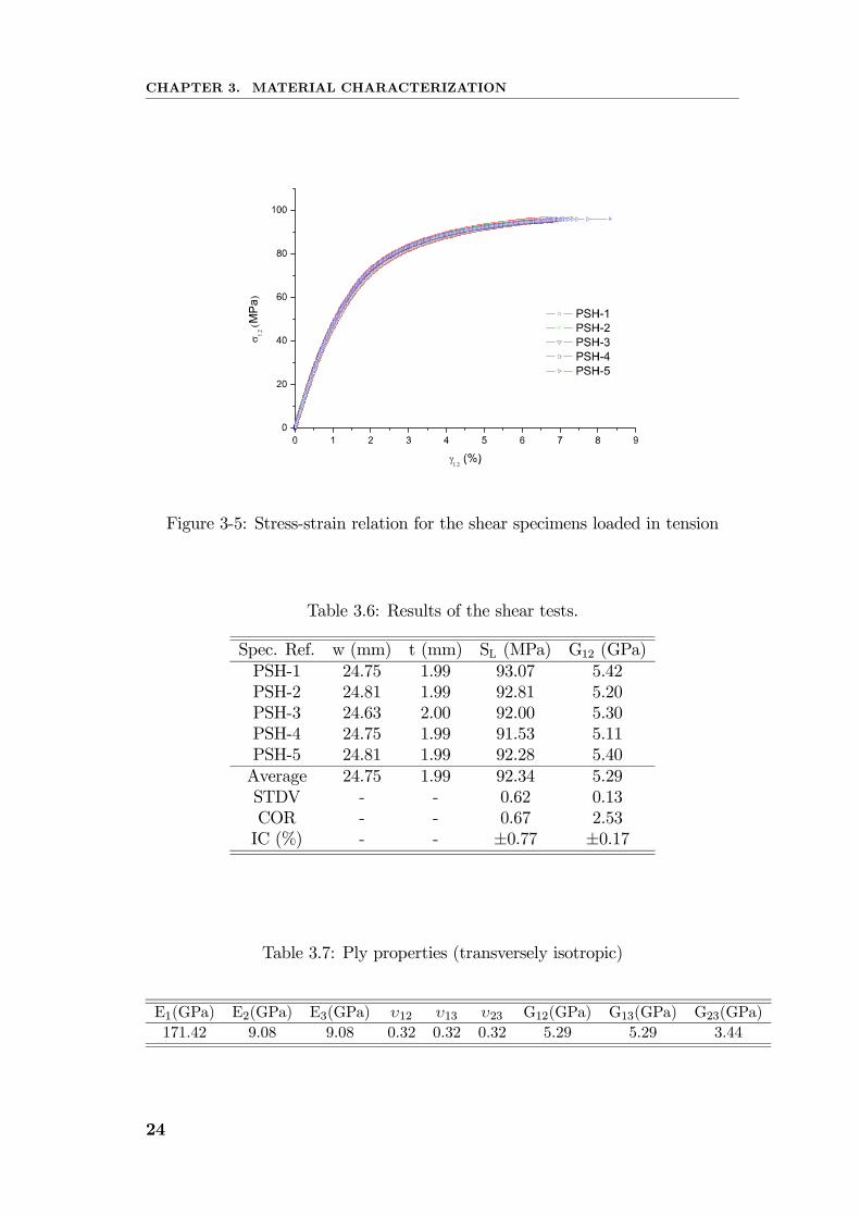
performed are shown in Figure 3-5. Table 3.6 shows the results obtained in the
shear tests. Table 3.7 summarizes the ply properties of the material, considering
a transversely isotropic behaviour.
22
3.4. STRAIN GAUGE BONDING
Table 3.4: Results of the transverse tensile test.
Spec. Ref. w (mm) t (mm) E2 (GPa) YT (MPa)PT90-1 24.72 1.99 9.02 -PT90-2 24.57 1.99 8.98 56.61PT90-3 24.67 1.99 9.04 60.05PT90-4 24.74 1.99 9.21 63.45PT90-5 24.75 1.98 9.13 69.03Average 24.69 1.99 9.08 62.29STDV - - 0.09 5.29COR - - 1.03 8.50IC (%) - - ±0.12 ±8.42
Table 3.5: Shear test matrix
Test Type Lay-up number of specimens Control type SpeedShear (45/− 45)4S 5 Displacement 1 mm/min
Coefficients of thermal expansion
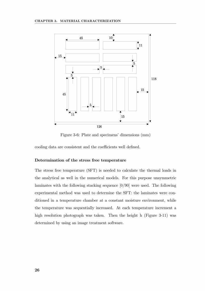
The experimental characterization of the composite’s CTEs, α11 and α22, was
performed according to the dilatometer’s manufacturer’s instructions. Specimens
with a section of 10x10mm2 were cut with a water jet machine from a unidirec-
tional plate as shown in Figure 3-6. The plate consisted of 76 unidirectional plies
which were carefully layed-up by hand and then hotpressed using the equipment
shown in Figure 3-2. As mentioned earlier, thicker laminates should be monitored
during cure and therefore two thermocouples were used for checking temperature
evolution. Before testing using the equipment shown in Figure 3-7, the specimens
were conditioned in an oven at 70 C for two hours, to remove absorved moisture
and reduce the level of residual stresses, as proposed in [26], [27]. The heat rates
are shown in Figure 3-8. Before the tests each specimen must be measured. The
respective lengths are shown in Table 3.8.
23
CHAPTER 3. MATERIAL CHARACTERIZATION
σ 12 (
)
γ12
Figure 3-5: Stress-strain relation for the shear specimens loaded in tension
Table 3.6: Results of the shear tests.
Spec. Ref. w (mm) t (mm) SL (MPa) G12 (GPa)PSH-1 24.75 1.99 93.07 5.42PSH-2 24.81 1.99 92.81 5.20PSH-3 24.63 2.00 92.00 5.30PSH-4 24.75 1.99 91.53 5.11PSH-5 24.81 1.99 92.28 5.40Average 24.75 1.99 92.34 5.29STDV - - 0.62 0.13COR - - 0.67 2.53IC (%) - - ±0.77 ±0.17
Table 3.7: Ply properties (transversely isotropic)
E1(GPa) E2(GPa) E3(GPa) υ12 υ13 υ23 G12(GPa) G13(GPa) G23(GPa)171.42 9.08 9.08 0.32 0.32 0.32 5.29 5.29 3.44
24
3.4. STRAIN GAUGE BONDING
Table 3.8: Measured parameters
Spec. Ref. L (mm) d (mm)CTEH-1 44.94 10.35CTEH-2 45.05 10.38CTEH-3 45.06 10.35CTEH-4 44.99 10.35CTEH-5 44.86 10.35CTET-1 45.08 10.35CTET-2 44.92 10.36CTET-3 45.12 10.37CTET-4 44.85 10.37CTET-5 45.10 10.39
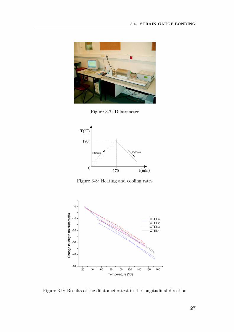
Table 3.9 shows the results for the coefficient of thermal expansion in the
fibres’ direction. The results of the tests are shown in Figures 3-9 and 3-10
Table 3.10 shows the results for the coefficient of thermal expansion transversal
Table 3.9: Results of the dilatomeric tests α11
Spec. Ref. w (mm) t (mm) Heat. Vel. α11 (10−6/oC)CTEL-1 10.00 10.00 1.00 -5.84CTEL-2 10.00 10.00 1.00 -4.67CTEL-3 10.00 10.00 1.00 -5.06CTEL-4 10.00 10.00 1.00 -6.35Average - - - -5.48STDV - - - 0.76COR - - - -13.81IC (%) - - - 1.05
to the fibres’ direction.
Hysteresis is observed after cool down of the specimens. It is generally thought
to be a result of the adhesive between the gauge and specimen being affected by
the heat. It is also possible that viscoelastic effects may influence the material
response of the composite at higher temperatures. Higher rates of temperature
change appear to produce more hysteresis, indicating that the material is not
in thermal equilibrium. However, at lower temperatures, the heating and the
25
CHAPTER 3. MATERIAL CHARACTERIZATION
Figure 3-6: Plate and specimens’ dimensions (mm)
cooling data are consistent and the coefficients well defined.
Determination of the stress free temperature
The stress free temperature (SFT) is needed to calculate the thermal loads in
the analytical as well in the numerical models. For this purpose unsymmetric
laminates with the following stacking sequence [0/90] were used. The following
experimental method was used to determine the SFT: the laminates were con-
ditioned in a temperature chamber at a constant moisture environment, while
the temperature was sequentially increased. At each temperature increment a
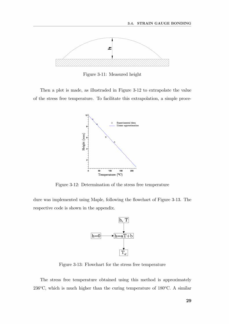
high resolution photograph was taken. Then the height h (Figure 3-11) was
determined by using an image treatment software.
26
3.4. STRAIN GAUGE BONDING
Figure 3-7: Dilatometer
Figure 3-8: Heating and cooling rates
Figure 3-9: Results of the dilatometer test in the longitudinal direction
27
CHAPTER 3. MATERIAL CHARACTERIZATION
Figure 3-10: Results of the dilatometer test in the transverse direction
Table 3.10: Results of the dilatomeric tests α22.
Spec. Ref. w (mm) t (mm) Heat. Vel. α22 (10−6/oC)CTET-1 10.00 10.00 1.00 25.70CTET-2 10.00 10.00 1.00 25.90CTET-3 10.00 10.00 1.00 25.56CTET-4 10.00 10.00 1.00 25.79CTET-5 10.00 10.00 1.00 26.25Average - - - 25.84STDV - - - 0.26COR - - - 1.01IC (%) - - - 0.32
28
3.4. STRAIN GAUGE BONDING
Figure 3-11: Measured height
Then a plot is made, as illustraded in Figure 3-12 to extrapolate the value
of the stress free temperature. To facilitate this extrapolation, a simple proce-
Figure 3-12: Determination of the stress free temperature
dure was implemented using Maple, following the flowchart of Figure 3-13. The
respective code is shown in the appendix.
Figure 3-13: Flowchart for the stress free temperature
The stress free temperature obtained using this method is approximately
236oC, which is much higher than the curing temperature of 180oC. A similar
29
CHAPTER 3. MATERIAL CHARACTERIZATION
experiment conducted by Flaggs et al. [28] gives a stress free temperature ap-
proximately 10oC higher than the curing temperature. This is due to the chemical
shrinkage of the resin which is never recovered. The reason for the results dispar-
ity of the procedure carried out in this work relies, certainly, on the measuring
method used: although the pictures taken were of great quality, there was some
difficulty in finding the reference points needed. Therefore all further calculations,
numerical and analytical, used the curing temperature of 180oC when needed.
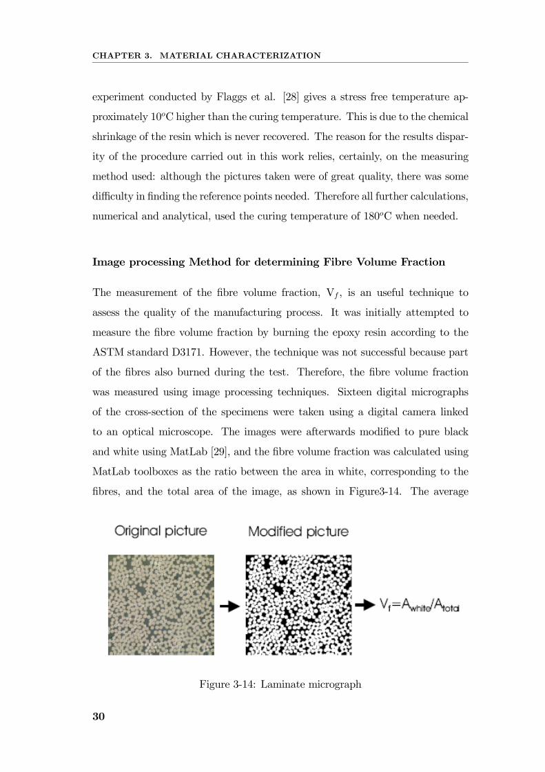
Image processing Method for determining Fibre Volume Fraction
The measurement of the fibre volume fraction, Vf , is an useful technique to
assess the quality of the manufacturing process. It was initially attempted to
measure the fibre volume fraction by burning the epoxy resin according to the
ASTM standard D3171. However, the technique was not successful because part
of the fibres also burned during the test. Therefore, the fibre volume fraction
was measured using image processing techniques. Sixteen digital micrographs
of the cross-section of the specimens were taken using a digital camera linked
to an optical microscope. The images were afterwards modified to pure black
and white using MatLab [29], and the fibre volume fraction was calculated using
MatLab toolboxes as the ratio between the area in white, corresponding to the
fibres, and the total area of the image, as shown in Figure3-14. The average
Figure 3-14: Laminate micrograph
30
3.4. STRAIN GAUGE BONDING
fibre volume fraction using the procedure mentioned above was 59.1 percent.
Using this information, the microscopic properties of the constituents, fibre and
matrix, may be obtained by applying the rule of mixtures. They will be needed for
the numerical simulations regarding a micro/mezoscale based model for residual
stress determination.
3.4.2 Micromechanical properties
In this section the moduli of the fibre and matrix were determined and compared
with the manufacturer’s values. The microscopic properties were needed for the
development of micromechanical models in Chapter 6. The following assumptions
are made: The fibers are:
• Homogeneous
• Linearly elastic
• Orthotropic
• Regularly spaced
• Perfectly aligned
• Perfectly bonded
The matrix is:
• Homogeneous
• Linearly elastic
• Isotropic
• Void-free
Equation (3.1) shows the rule of mixtures, which represents a linear behaviour of
the apparent Young’s modulus, E1, from Em to Ef as Vf varies from 0 to 1.
E1 = Ef × Vf +Em × Vm (3.1)
31
CHAPTER 3. MATERIAL CHARACTERIZATION
where Vf and Vm are the fiber and matrix volume fractions, respectively. Obvi-
ously, they are related to each other by Equation (3.2).
Vf = 1− Vm (3.2)
Regarding the Young’s modulus in the transverse direction, E2, it is defined as
follows:1
E2=
VfEf+
VmEm
(3.3)
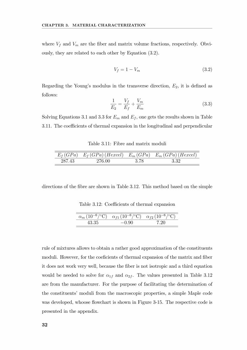
Solving Equations 3.1 and 3.3 for Em and Ef , one gets the results shown in Table
3.11. The coefficients of thermal expansion in the longitudinal and perpendicular
Table 3.11: Fibre and matrix moduli
Ef (GPa) Ef (GPa) (Hexcel) Em (GPa) Em (GPa) (Hexcel)287.43 276.00 3.78 3.32
directions of the fibre are shown in Table 3.12. This method based on the simple
Table 3.12: Coefficients of thermal expansion
αm (10−6/C) αf1 (10
−6/C) αf2 (10−6/C)
43.35 −0.90 7.20
rule of mixtures allows to obtain a rather good approximation of the constituents
moduli. However, for the coeficients of thermal expansion of the matrix and fiber
it does not work very well, because the fiber is not isotropic and a third equation
would be needed to solve for α1f and α2f . The values presented in Table 3.12
are from the manufacturer. For the purpose of facilitating the determination of
the constituents’ moduli from the macroscopic properties, a simple Maple code
was developed, whoose flowchart is shown in Figure 3-15. The respective code is
presented in the appendix.
32
3.5. MANUFACTURE OF SPECIMENS FOR HOLE DRILLING AND
HYGROTHERMAL TESTS
Figure 3-15: Flowchart for the determination of microscopic properties
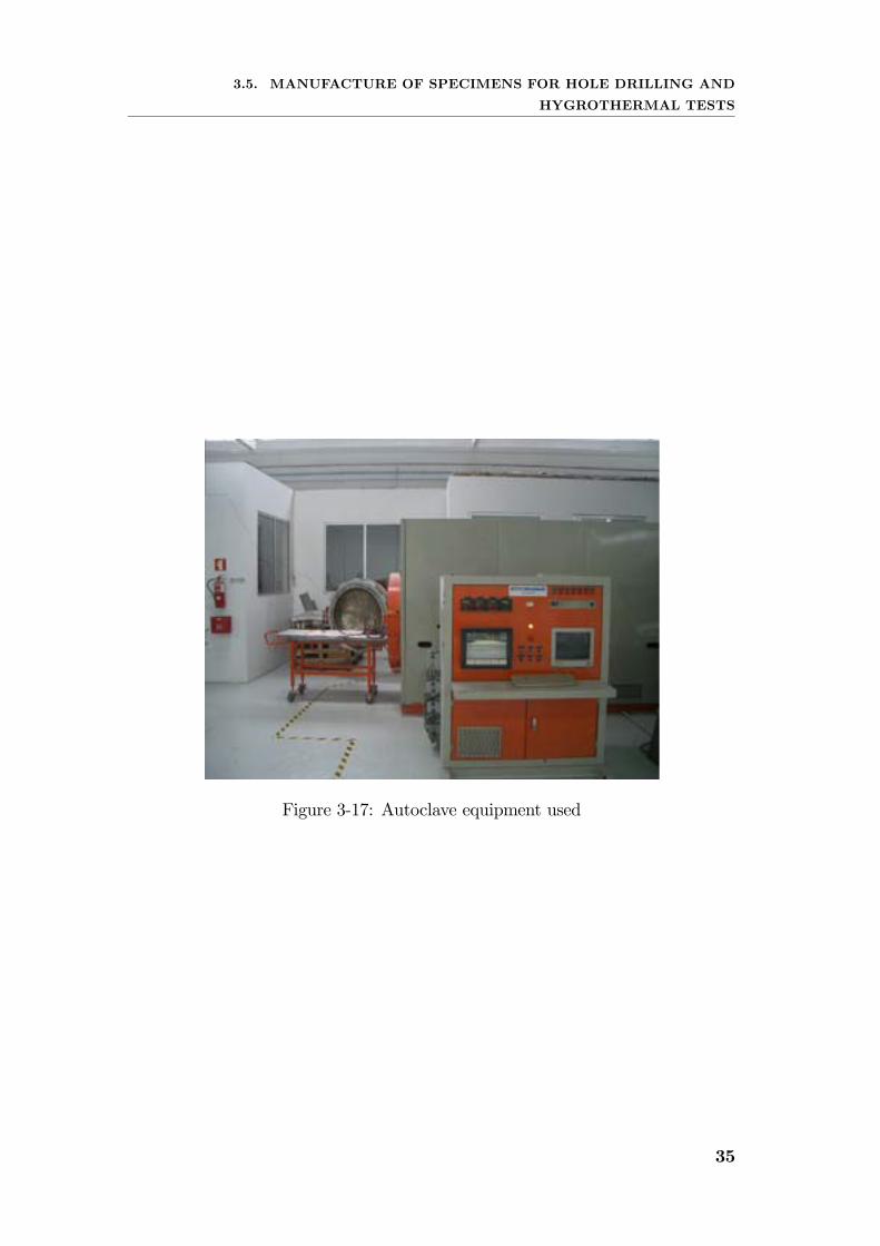
3.5 Manufacture of specimens for hole drilling
and hygrothermal tests
In this section the manufacturing process of the specimens for the hole drilling
method and the water absorption tests is described. After an unsuccessfull at-
tempt to produce the rather thin specimens using the hot press, it was decided
to use an autoclave instead. For specimens with few layers it would be necessary
to use a very thin steel sheet to control the thickness of the specimens and to
avoid excessive resin flow. Also, the use of an autoclave allows for simultane-
ous production of specimens with different stacking sequences, thus increasing
productivity.
3.5.1 Specimens’ specifications and manufacture
Table 3.13 shows all the specifications regarding the specimens used in the hole
drilling method.
Table 3.13: Specimen characterisitcs for the hole drilling experiments
Spec. Ref. Lay-up Specimens Qty. Thickness (mm)HDM0 [02/902]s 1 1.048HDM1 [02/902]s 1 1.048HDM2 [02/902]s 1 1.048
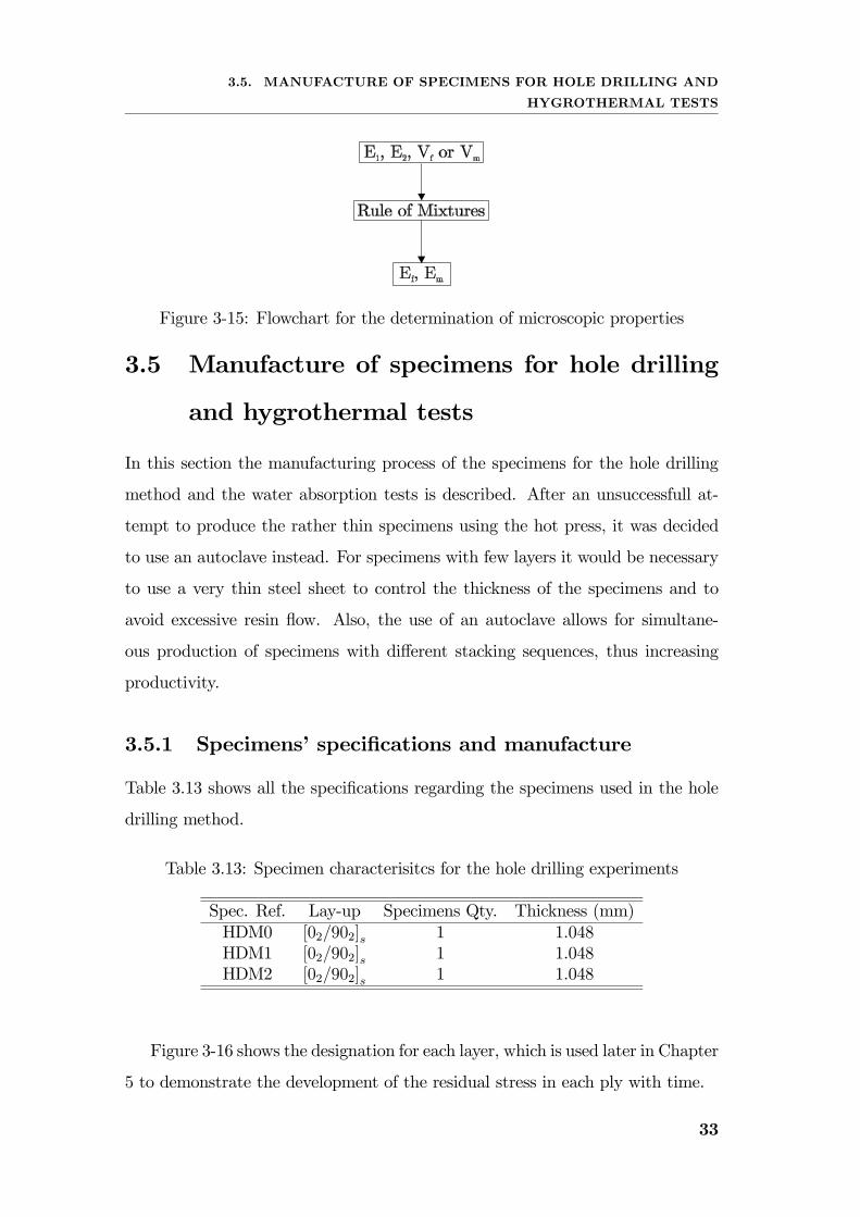
Figure 3-16 shows the designation for each layer, which is used later in Chapter
5 to demonstrate the development of the residual stress in each ply with time.
33
CHAPTER 3. MATERIAL CHARACTERIZATION
Figure 3-16: Ply designation
Table 3.14 shows all the specifications regarding the specimens used in the
hygrothermal experiments. Unlike the specimens used to determine basic mate-
Table 3.14: Specimen characterisitcs for the moisture absorption experiments
Spec. Ref. Lay-up Specimens Qty. Thickness (mm)MST1 [0/90] 5 0.262MST2 [0/902] 5 0.393MST3 [0/904] 5 0.655MST4 [90/0/903] 5 0.655
rial properties, an autoclave is used to produce the test specimens. The curing
cycle is the same, as shown in Figure 3-1. Autoclave processing is used for the
manufacture of superior quality structural components containing high fibre vol-
ume and low void contents. The autoclave is a pressure vessel which provides the
curing conditions for the composite where the application of vacuum, pressure,
heat up rate and cure temperature are controlled. Also, productivity is drasti-
cally increased, allowing a large amount of specimens with different sizes to be
simultaneously manufactured, while maintaining the same quality.
34
3.5. MANUFACTURE OF SPECIMENS FOR HOLE DRILLING AND
HYGROTHERMAL TESTS
Figure 3-17: Autoclave equipment used
35

36
Chapter 4
Analytical Determination of
Residual Stresses
Residual stresses may be predicted by the classical laminate theory at the macro-
scopic level. However, when large displacements are involved, such as out-of-
plane displacements in unsymmetric laminates, classical laminate theory alone is
unable to correctly predict such shapes. The algorithm implemented here was
used to determine the residual stress state according to the CLT at the ply level
immediately after manufacture of the cross-ply specimens.
4.1 Stress-Srain relations of an individual ply
within a laminate
The plane stress constitutive relation of ply k is established as:⎡⎢⎢⎢⎣σx
σy
τ s
⎤⎥⎥⎥⎦k
=
⎡⎢⎢⎢⎣Qxx Qxy Qxs
Qyx Qyy Qys
Qsx Qsy Qss
⎤⎥⎥⎥⎦k
⎡⎢⎢⎢⎣x
y
γs
⎤⎥⎥⎥⎦k
(4.1)
37
CHAPTER 4. ANALYTICAL DETERMINATION OF RESIDUAL STRESSES
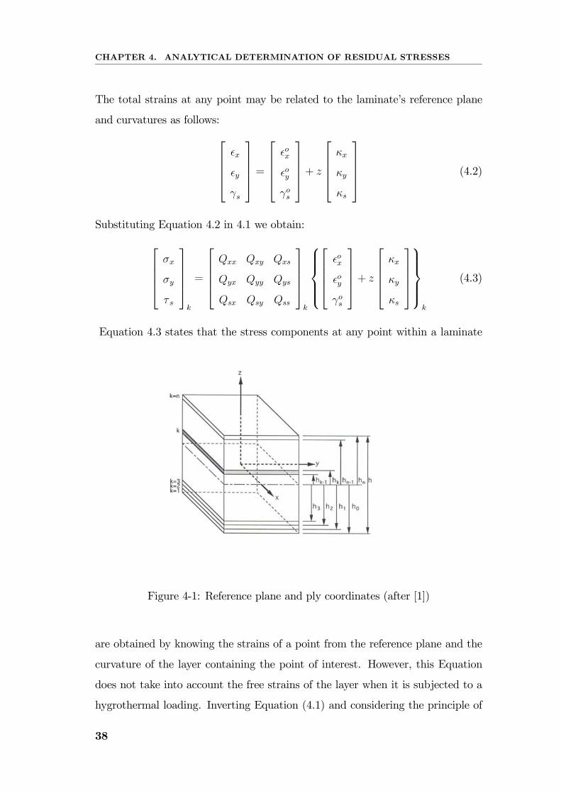
The total strains at any point may be related to the laminate’s reference plane
and curvatures as follows:⎡⎢⎢⎢⎣x
y
γs
⎤⎥⎥⎥⎦ =⎡⎢⎢⎢⎣
ox
oy
γos
⎤⎥⎥⎥⎦+ z
⎡⎢⎢⎢⎣κx
κy
κs
⎤⎥⎥⎥⎦ (4.2)
Substituting Equation 4.2 in 4.1 we obtain:⎡⎢⎢⎢⎣σx
σy
τ s
⎤⎥⎥⎥⎦k
=
⎡⎢⎢⎢⎣Qxx Qxy Qxs
Qyx Qyy Qys
Qsx Qsy Qss
⎤⎥⎥⎥⎦k
⎧⎪⎪⎪⎨⎪⎪⎪⎩⎡⎢⎢⎢⎣
ox
oy
γos
⎤⎥⎥⎥⎦+ z
⎡⎢⎢⎢⎣κx
κy
κs
⎤⎥⎥⎥⎦⎫⎪⎪⎪⎬⎪⎪⎪⎭
k
(4.3)
Equation 4.3 states that the stress components at any point within a laminate
Figure 4-1: Reference plane and ply coordinates (after [1])
are obtained by knowing the strains of a point from the reference plane and the
curvature of the layer containing the point of interest. However, this Equation
does not take into account the free strains of the layer when it is subjected to a
hygrothermal loading. Inverting Equation (4.1) and considering the principle of
38
4.1. STRESS-SRAIN RELATIONS OF AN INDIVIDUAL PLY WITHIN A
LAMINATE
strain superposition within a laminate:⎡⎢⎢⎢⎣x
y
γs
⎤⎥⎥⎥⎦k
=
⎡⎢⎢⎢⎣Sxx Sxy Sxs
Syx Syy Sys
Ssx Ssy Sss
⎤⎥⎥⎥⎦k
⎡⎢⎢⎢⎣σx
σy
τ s
⎤⎥⎥⎥⎦k
+
⎡⎢⎢⎢⎣εx
εy
εs
⎤⎥⎥⎥⎦k
(4.4)
In layer k the total strains [ ]kx,y equalize the sum of the strains produced by
the existing stresses in the layer, [σ]kx,y, and the free unconstrained strains [ε]kx,y.
Inverting Equation (4.4) gives the stresses in any layer k as follows:
⎡⎢⎢⎢⎣σx
σy
τ s
⎤⎥⎥⎥⎦k
=
⎡⎢⎢⎢⎣Qxx Qxy Qxs
Qyx Qyy Qys
Qsx Qsy Qss
⎤⎥⎥⎥⎦k
⎡⎢⎢⎢⎣x − εx
y − εy
γs − εs
⎤⎥⎥⎥⎦k
(4.5)
Taking Equation (4.2) into account, one obtains the following more generalized
equation: ⎡⎢⎢⎢⎣σx
σy
τ s
⎤⎥⎥⎥⎦k
=
⎡⎢⎢⎢⎣Qxx Qxy Qxs
Qyx Qyy Qys
Qsx Qsy Qss
⎤⎥⎥⎥⎦k
⎡⎢⎢⎢⎣ox + zκx − εx
oy + zκy − εy
γos + zκs − εs
⎤⎥⎥⎥⎦k
(4.6)
In the following section the procedure for the determination of residual stresses
owing to thermal effects only is thoroughly explained. It was implemented using
the software Maple 9.5 [30].
4.1.1 Analytical Procedure for RTS Determination
The strains due to the thermal difference ∆T are first determined using Equation
4.7. ⎡⎢⎢⎢⎣εx
εy
εs
⎤⎥⎥⎥⎦k
=
⎡⎢⎢⎢⎣αx
αy
αs
⎤⎥⎥⎥⎦k
∆T (4.7)
39
CHAPTER 4. ANALYTICAL DETERMINATION OF RESIDUAL STRESSES
The thermal loads are calculated for the laminate as follows:⎡⎢⎢⎢⎣NHT
x
NHTy
NHTs
⎤⎥⎥⎥⎦ =nX
k=1
⎡⎢⎢⎢⎣Qxx Qxy Qxs
Qyx Qyy Qys
Qsx Qsy Qss
⎤⎥⎥⎥⎦k
⎡⎢⎢⎢⎣εx
εy
εs
⎤⎥⎥⎥⎦k
tk (4.8)
For the thermal moments:⎡⎢⎢⎢⎣MHT
x
MHTy
MHTs
⎤⎥⎥⎥⎦ =nX
k=1
⎡⎢⎢⎢⎣Qxx Qxy Qxs
Qyx Qyy Qys
Qsx Qsy Qss
⎤⎥⎥⎥⎦k
⎡⎢⎢⎢⎣εx
εy
εs
⎤⎥⎥⎥⎦k
zktk (4.9)
where tk and zk are the layer’s thickness and distance to the reference plane.
The results of Equations (4.8) and (4.9) are used to calculate the reference plane
strains and the laminate’s curvatures, as shown in Equations (4.10) and (4.11).
⎡⎢⎢⎢⎣ox
oy
γos
⎤⎥⎥⎥⎦k
=
⎡⎢⎢⎢⎣axx axy axs
ayx ayy ays
asx asy ass
⎤⎥⎥⎥⎦k
⎡⎢⎢⎢⎣NHT
x
NHTy
NHTs
⎤⎥⎥⎥⎦+⎡⎢⎢⎢⎣
bxx bxy bxs
byx byy bys
bsx bsy bss
⎤⎥⎥⎥⎦k
⎡⎢⎢⎢⎣MHT
x
MHTy
MHTs
⎤⎥⎥⎥⎦ (4.10)
⎡⎢⎢⎢⎣κx
κy
κs
⎤⎥⎥⎥⎦k
=
⎡⎢⎢⎢⎣cxx cxy cxs
cyx cyy cys
csx csy css
⎤⎥⎥⎥⎦k
⎡⎢⎢⎢⎣NHT
x
NHTy
NHTs
⎤⎥⎥⎥⎦+⎡⎢⎢⎢⎣
dxx dxy dxs
dyx dyy dys
dsx dsy dss
⎤⎥⎥⎥⎦k
⎡⎢⎢⎢⎣MHT
x
MHTy
MHTs
⎤⎥⎥⎥⎦ (4.11)
The total strains are determined using Equation (4.2). The residual stresses are
then calculated by means of Equation (4.5).
4.1.2 Maple code for the CLT implementation
The Maple code used is explained in the appendix. Although there are other
well developed programmes based on the CLT [31], the procedures illustrated
below were used and may serve as a basis for future development of analytical
tools using mathematical computation programmes like Maple. Figure 4-2 shows
the flowchart including all the data inputs needed by the algorithm. Although
40
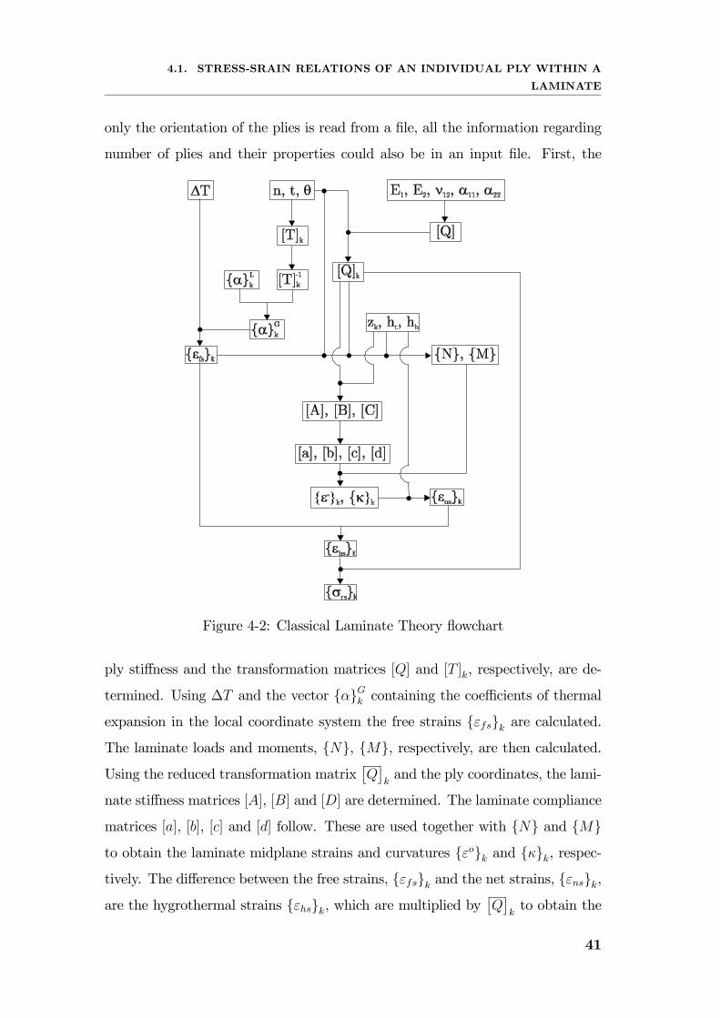
4.1. STRESS-SRAIN RELATIONS OF AN INDIVIDUAL PLY WITHIN A
LAMINATE
only the orientation of the plies is read from a file, all the information regarding
number of plies and their properties could also be in an input file. First, the
Figure 4-2: Classical Laminate Theory flowchart
ply stiffness and the transformation matrices [Q] and [T ]k, respectively, are de-
termined. Using ∆T and the vector αGk containing the coefficients of thermal
expansion in the local coordinate system the free strains εfsk are calculated.
The laminate loads and moments, N, M, respectively, are then calculated.
Using the reduced transformation matrix£Q¤kand the ply coordinates, the lami-
nate stiffness matrices [A], [B] and [D] are determined. The laminate compliance
matrices [a], [b], [c] and [d] follow. These are used together with N and M
to obtain the laminate midplane strains and curvatures εok and κk, respec-
tively. The difference between the free strains, εfsk and the net strains, εnsk,
are the hygrothermal strains εhsk, which are multiplied by£Q¤kto obtain the
41

CHAPTER 4. ANALYTICAL DETERMINATION OF RESIDUAL STRESSES
residual stresses vector σrsk for each ply.
42
Chapter 5
Experimental Procedures
The hole drilling method applied to orthotropic materials as described in reference
[22] is used for the determination of residual stresses in symmetric laminates. A
detailed description of the method is presented in this Chapter.
5.1 Theoretical formulation
The model used to determine the residual stress distribution is based on the
assumptions indicated bellow:
• the material is elastic and orthotropic
• the stress component (σzz) perpendicular to the surface is very small
Sicot [22] adapted a previous work developed by Soete [32] and Lake [33]
to the case of orthotropic materials and also the incremental character of the
hole drilling method and the consequent redistribution of the stresses after each
increment.
The change in strain at any location, for a fixed radial distance from the centre
of the hole, can be described by the following equation:
εin (θi) = Ain (σ1hi + σ2hi) + (σ1hi − σ2hi) (Bin cos(2θi) + Cin sin(2θi)) (5.1)
43
CHAPTER 5. EXPERIMENTAL PROCEDURES
where εin is the strain contribution of layer i for the total strain measured at the
nth increment, σ1hi and σ2hi are the main residual stresses in layer i (the depth
of the layer is hi), θi is the angle between the reference gauge and the first main
direction of residual stress and Ain, Bin and Cin are the calibration coefficients
for the nth increment and loading on the ith layer.
The strain measurements in three directions are used to determine the three
unknown factors σ1hi, σ2hi and θi for each drilling increment. For example, when
the first increment is drilled (hi=h1), the strain is obtained for the three directions
corresponding to the orientations of the strain gauges:
⎧⎪⎪⎪⎨⎪⎪⎪⎩ε111 (θ1) = A11 (σ1h1 + σ2h1) + (σ1h1 − σ2h1) (B11 cos(2θ1) + C11 sin(2θ1))
ε211 (θ1) = A11 (σ1h1 + σ2h1) + (σ1h1 − σ2h1) (B11 cos(2(θ1 + α)) + C11 sin(2(θ1 + α)))
ε311 (θ1) = A11 (σ1h1 + σ2h1) + (σ1h1 − σ2h1) (B11 cos(2(θ1 + β)) + C11 sin(2(θ1 + β)))
(5.2)
where εj11 is the contribution in the jth direction and α and β are the angles of
the 2nd and 3rd direction of measurement.
After the nth increment the total depth becomes hn and the equations be-
come:
⎧⎪⎪⎪⎨⎪⎪⎪⎩ε1nn (θn) = Ann (σ1hn + σ2hn) + (σ1hn − σ2hn) (Bnn cos(2θn) + Cnn sin(2θn))
ε2nn (θn) = Ann (σ1hn + σ2hn) + (σ1hn − σ2hn) (Bnn cos(2(θn + α)) + Cnn sin(2(θn + α)))
ε3nn (θn) = Ann (σ1hn + σ2hn) + (σ1hn − σ2hn) (Bnn cos(2(θn + β)) + Cnn sin(2(θn + β)))
(5.3)
However, after the first increment, the change in the hole geometry must also
be taken into account. Each previously removed layer affects the total strain
measured on the surface. So the strain measured on the surface due to the
removed layer only is expressed as follows (to simplify εjnn = εjn):
ε1n = ε1mn −n−1Xi=1
ε1in (5.4)
44
5.1. THEORETICAL FORMULATION
ε2n = ε2mn −n−1Xi=1
ε2in (5.5)
ε3n = ε3mn −n−1Xi=1
ε3in (5.6)
where εjin is the contribution of the i layer in j direction in the case of the nth
increment and εjmn is the total strain measured on the surface by the strain gauges
in the j direction.
For example, after three increments the resulting expression is:
ε13 = ε1m3 −2X
i=1
ε1i3 = ε1m3 −¡ε113 + ε123
¢(5.7)
After substituting in Equation (5.1):
ε13 = ε1m3 −[(A13 (σ1h1 + σ2h1) + (σ1h1 − σ2h1) (B13 cos(2θ1) + C13 sin(2θ1)))+
+(A23 (σ1h2 + σ2h2) + (σ1h2 − σ2h2) (B23 cos(2θ2) + C23 sin(2θ2)))]
(5.8)
With this method Sicot [22] considers that for each increment the total strain
measured on the surface can be divided into two parts:
• the first is due to the residual stress on the removed layer
• the second is the contribution of the residual stress redistribution caused
by the change in geometry.
For a strain gauge similar to the one shown in Figure 5-2, three equations are
obtained for each drilling increment by reversing the system as follows:
σ1hn =ε1n (Ann −Bnn sin 2θn + Cnn cos 2θn)− ε2n (Ann −Bnn cos 2θn − Cnn cos 2θn)
2AnnBnn (− sin 2θn + cos 2θn) + 2AnnCnn (sin 2θn + cos 2θn)(5.9)
σ2hn =−ε1n (Ann +Bnn sin 2θn − Cnn cos 2θn) + ε2n (Ann +Bnn cos 2θn + Cnn cos 2θn)
2AnnBnn (− sin 2θn + cos 2θn) + 2AnnCnn (sin 2θn + cos 2θn)(5.10)
45
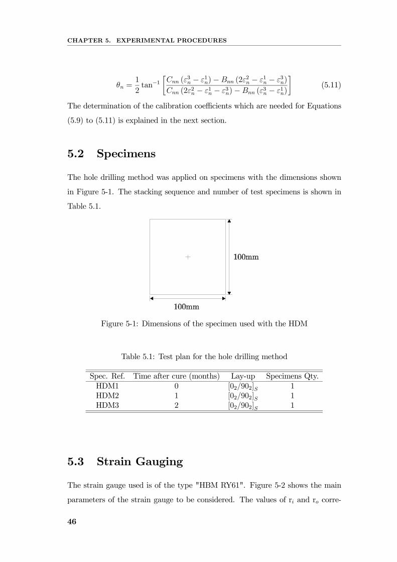
CHAPTER 5. EXPERIMENTAL PROCEDURES
θn =1
2tan−1
∙Cnn (ε
3n − ε1n)−Bnn (2ε
2n − ε1n − ε3n)
Cnn (2ε2n − ε1n − ε3n)−Bnn (ε3n − ε1n)
¸(5.11)
The determination of the calibration coefficients which are needed for Equations
(5.9) to (5.11) is explained in the next section.
5.2 Specimens
The hole drilling method was applied on specimens with the dimensions shown
in Figure 5-1. The stacking sequence and number of test specimens is shown in
Table 5.1.
Figure 5-1: Dimensions of the specimen used with the HDM
Table 5.1: Test plan for the hole drilling method
Spec. Ref. Time after cure (months) Lay-up Specimens Qty.HDM1 0 [02/902]S 1HDM2 1 [02/902]S 1HDM3 2 [02/902]S 1
5.3 Strain Gauging
The strain gauge used is of the type "HBM RY61". Figure 5-2 shows the main
parameters of the strain gauge to be considered. The values of ri and ro corre-
46
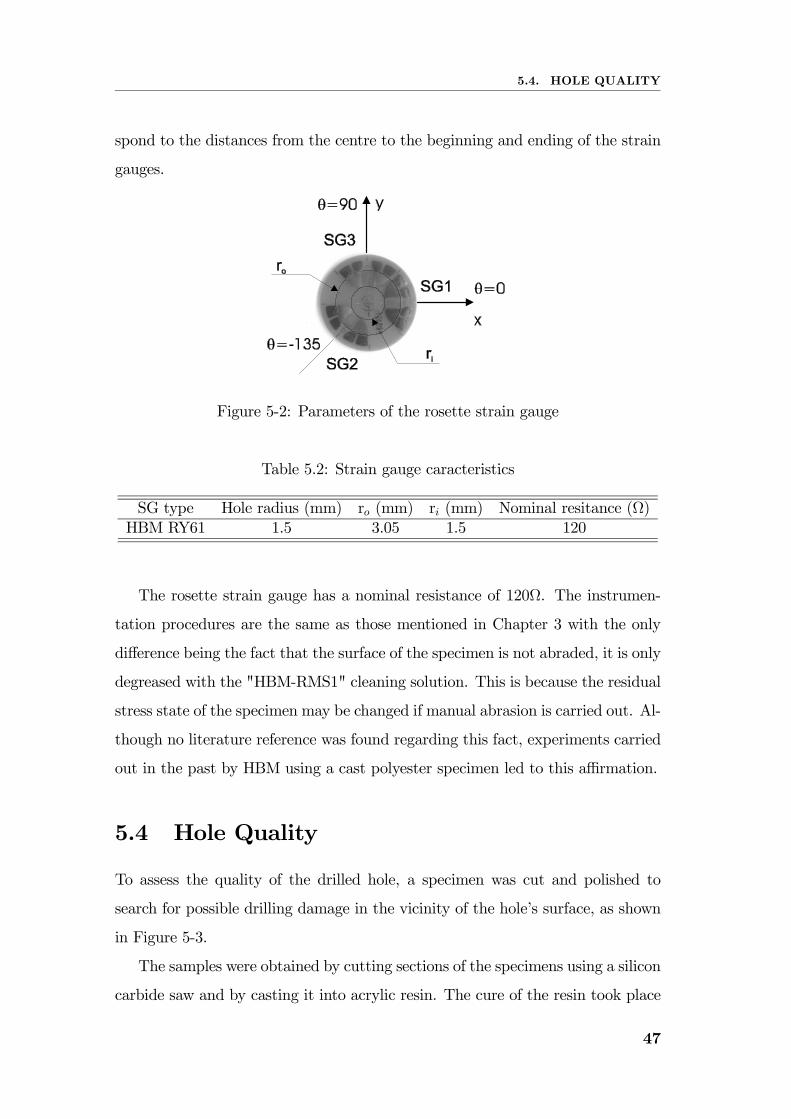
5.4. HOLE QUALITY
spond to the distances from the centre to the beginning and ending of the strain
gauges.
Figure 5-2: Parameters of the rosette strain gauge
Table 5.2: Strain gauge caracteristics
SG type Hole radius (mm) ro (mm) ri (mm) Nominal resitance (Ω)HBM RY61 1.5 3.05 1.5 120
The rosette strain gauge has a nominal resistance of 120Ω. The instrumen-
tation procedures are the same as those mentioned in Chapter 3 with the only
difference being the fact that the surface of the specimen is not abraded, it is only
degreased with the "HBM-RMS1" cleaning solution. This is because the residual
stress state of the specimen may be changed if manual abrasion is carried out. Al-
though no literature reference was found regarding this fact, experiments carried
out in the past by HBM using a cast polyester specimen led to this affirmation.
5.4 Hole Quality
To assess the quality of the drilled hole, a specimen was cut and polished to
search for possible drilling damage in the vicinity of the hole’s surface, as shown
in Figure 5-3.
The samples were obtained by cutting sections of the specimens using a silicon
carbide saw and by casting it into acrylic resin. The cure of the resin took place
47
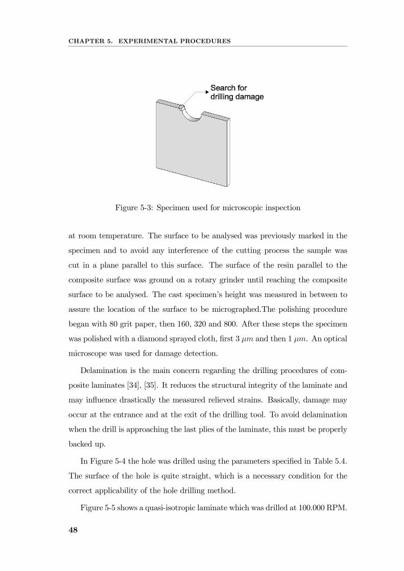
CHAPTER 5. EXPERIMENTAL PROCEDURES
Figure 5-3: Specimen used for microscopic inspection
at room temperature. The surface to be analysed was previously marked in the
specimen and to avoid any interference of the cutting process the sample was
cut in a plane parallel to this surface. The surface of the resin parallel to the
composite surface was ground on a rotary grinder until reaching the composite
surface to be analysed. The cast specimen’s height was measured in between to
assure the location of the surface to be micrographed.The polishing procedure
began with 80 grit paper, then 160, 320 and 800. After these steps the specimen
was polished with a diamond sprayed cloth, first 3 µm and then 1 µm. An optical
microscope was used for damage detection.
Delamination is the main concern regarding the drilling procedures of com-
posite laminates [34], [35]. It reduces the structural integrity of the laminate and
may influence drastically the measured relieved strains. Basically, damage may
occur at the entrance and at the exit of the drilling tool. To avoid delamination
when the drill is approaching the last plies of the laminate, this must be properly
backed up.
In Figure 5-4 the hole was drilled using the parameters specified in Table 5.4.
The surface of the hole is quite straight, which is a necessary condition for the
correct applicability of the hole drilling method.
Figure 5-5 shows a quasi-isotropic laminate which was drilled at 100.000 RPM.
48
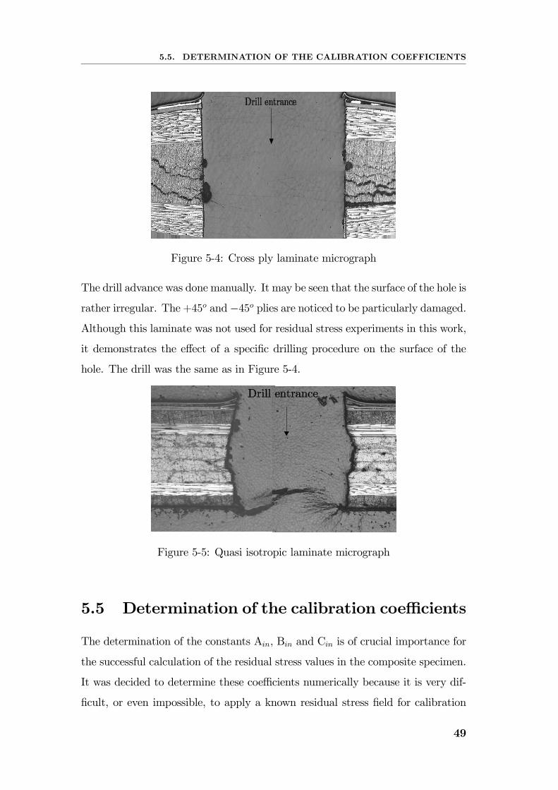
5.5. DETERMINATION OF THE CALIBRATION COEFFICIENTS
Figure 5-4: Cross ply laminate micrograph
The drill advance was done manually. It may be seen that the surface of the hole is
rather irregular. The+45o and−45o plies are noticed to be particularly damaged.
Although this laminate was not used for residual stress experiments in this work,
it demonstrates the effect of a specific drilling procedure on the surface of the
hole. The drill was the same as in Figure 5-4.
Figure 5-5: Quasi isotropic laminate micrograph
5.5 Determination of the calibration coefficients
The determination of the constants Ain, Bin and Cin is of crucial importance for
the successful calculation of the residual stress values in the composite specimen.
It was decided to determine these coefficients numerically because it is very dif-
ficult, or even impossible, to apply a known residual stress field for calibration
49
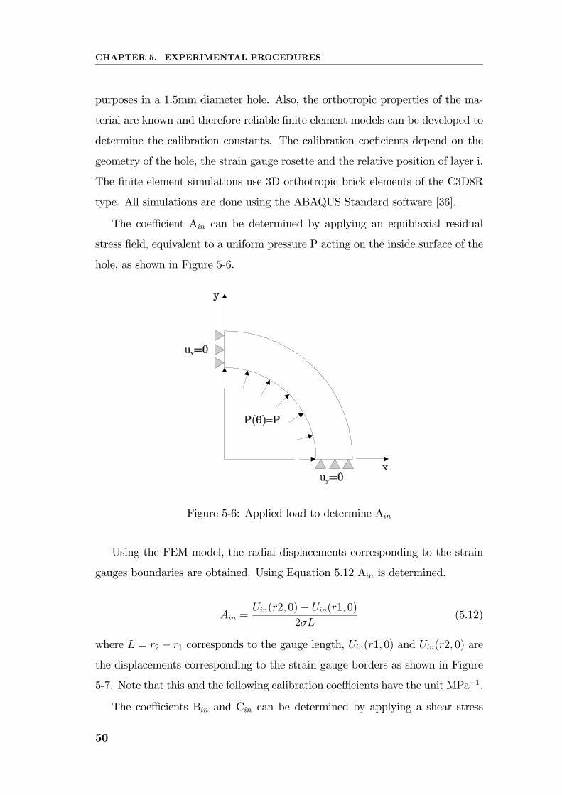
CHAPTER 5. EXPERIMENTAL PROCEDURES
purposes in a 1.5mm diameter hole. Also, the orthotropic properties of the ma-
terial are known and therefore reliable finite element models can be developed to
determine the calibration constants. The calibration coeficients depend on the
geometry of the hole, the strain gauge rosette and the relative position of layer i.
The finite element simulations use 3D orthotropic brick elements of the C3D8R
type. All simulations are done using the ABAQUS Standard software [36].
The coefficient Ain can be determined by applying an equibiaxial residual
stress field, equivalent to a uniform pressure P acting on the inside surface of the
hole, as shown in Figure 5-6.
Figure 5-6: Applied load to determine Ain
Using the FEM model, the radial displacements corresponding to the strain
gauges boundaries are obtained. Using Equation 5.12 Ain is determined.
Ain =Uin(r2, 0)− Uin(r1, 0)
2σL(5.12)
where L = r2 − r1 corresponds to the gauge length, Uin(r1, 0) and Uin(r2, 0) are
the displacements corresponding to the strain gauge borders as shown in Figure
5-7. Note that this and the following calibration coefficients have the unit MPa−1.
The coefficients Bin and Cin can be determined by applying a shear stress
50
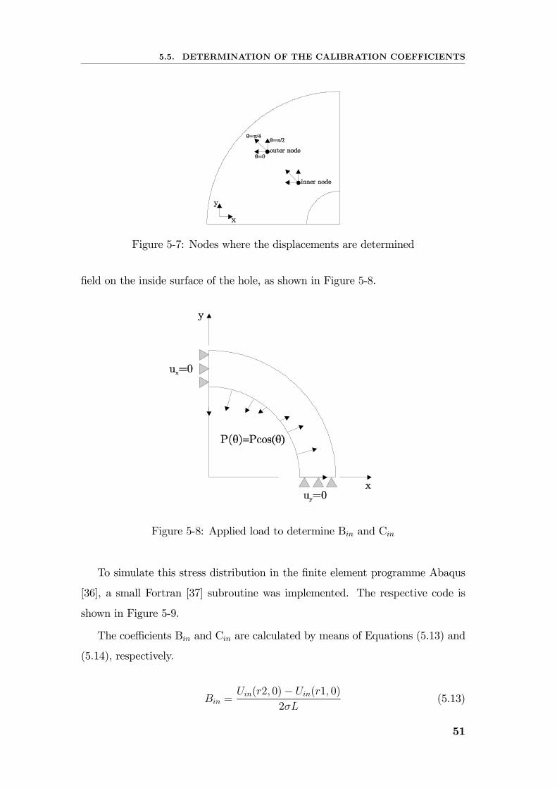
5.5. DETERMINATION OF THE CALIBRATION COEFFICIENTS
Figure 5-7: Nodes where the displacements are determined
field on the inside surface of the hole, as shown in Figure 5-8.
Figure 5-8: Applied load to determine Bin and Cin
To simulate this stress distribution in the finite element programme Abaqus
[36], a small Fortran [37] subroutine was implemented. The respective code is
shown in Figure 5-9.
The coefficients Bin and Cin are calculated by means of Equations (5.13) and
(5.14), respectively.
Bin =Uin(r2, 0)− Uin(r1, 0)
2σL(5.13)
51
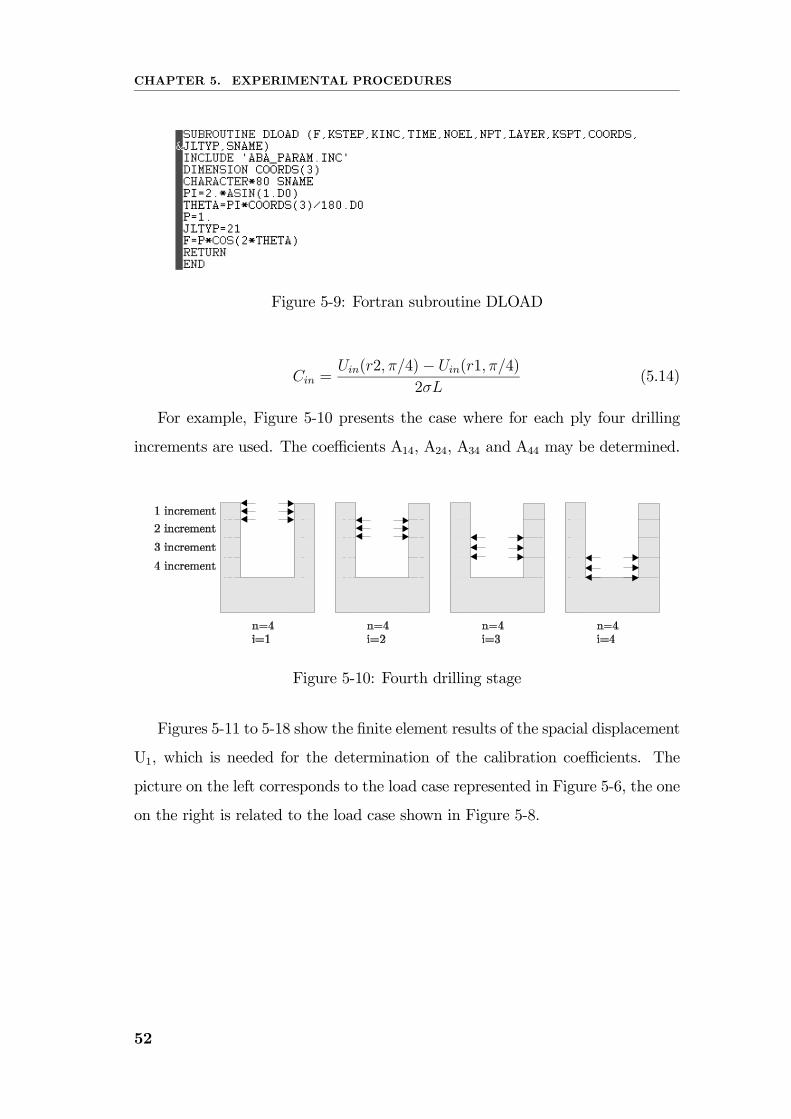
CHAPTER 5. EXPERIMENTAL PROCEDURES
Figure 5-9: Fortran subroutine DLOAD
Cin =Uin(r2, π/4)− Uin(r1, π/4)
2σL(5.14)
For example, Figure 5-10 presents the case where for each ply four drilling
increments are used. The coefficients A14, A24, A34 and A44 may be determined.
Figure 5-10: Fourth drilling stage
Figures 5-11 to 5-18 show the finite element results of the spacial displacement
U1, which is needed for the determination of the calibration coefficients. The
picture on the left corresponds to the load case represented in Figure 5-6, the one
on the right is related to the load case shown in Figure 5-8.
52
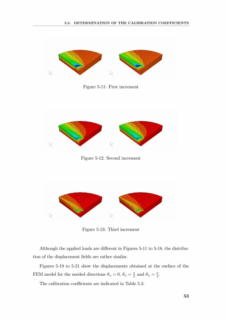
5.5. DETERMINATION OF THE CALIBRATION COEFFICIENTS
Figure 5-11: First increment
Figure 5-12: Second increment
Figure 5-13: Third increment
Although the applied loads are different in Figures 5-11 to 5-18, the distribu-
tion of the displacement fields are rather similar.
Figures 5-19 to 5-21 show the displacements obtained at the surface of the
FEM model for the needed directions θn = 0, θn = π2and θn =
π4.
The calibration coefficients are indicated in Table 5.3.
53
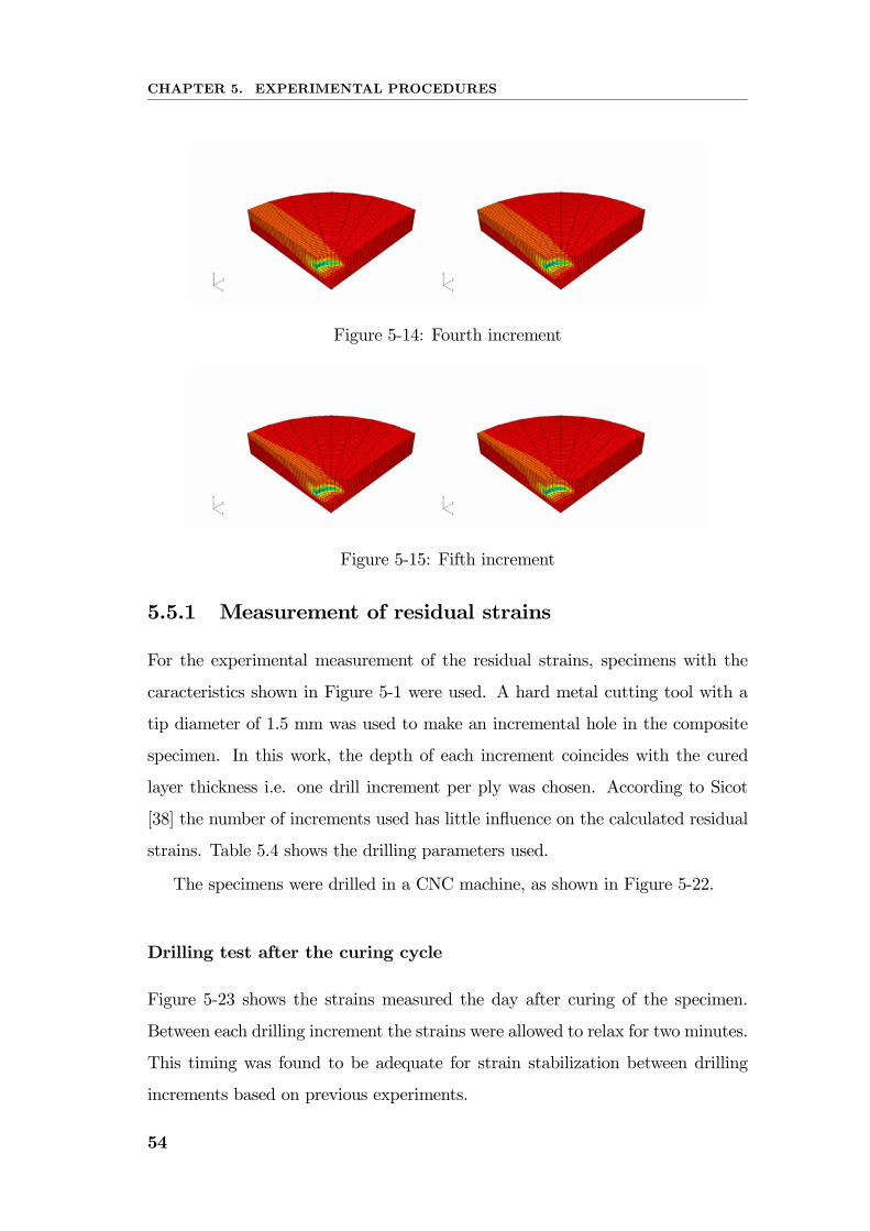
CHAPTER 5. EXPERIMENTAL PROCEDURES
Figure 5-14: Fourth increment
Figure 5-15: Fifth increment
5.5.1 Measurement of residual strains
For the experimental measurement of the residual strains, specimens with the
caracteristics shown in Figure 5-1 were used. A hard metal cutting tool with a
tip diameter of 1.5 mm was used to make an incremental hole in the composite
specimen. In this work, the depth of each increment coincides with the cured
layer thickness i.e. one drill increment per ply was chosen. According to Sicot
[38] the number of increments used has little influence on the calculated residual
strains. Table 5.4 shows the drilling parameters used.
The specimens were drilled in a CNC machine, as shown in Figure 5-22.
Drilling test after the curing cycle
Figure 5-23 shows the strains measured the day after curing of the specimen.
Between each drilling increment the strains were allowed to relax for two minutes.
This timing was found to be adequate for strain stabilization between drilling
increments based on previous experiments.
54
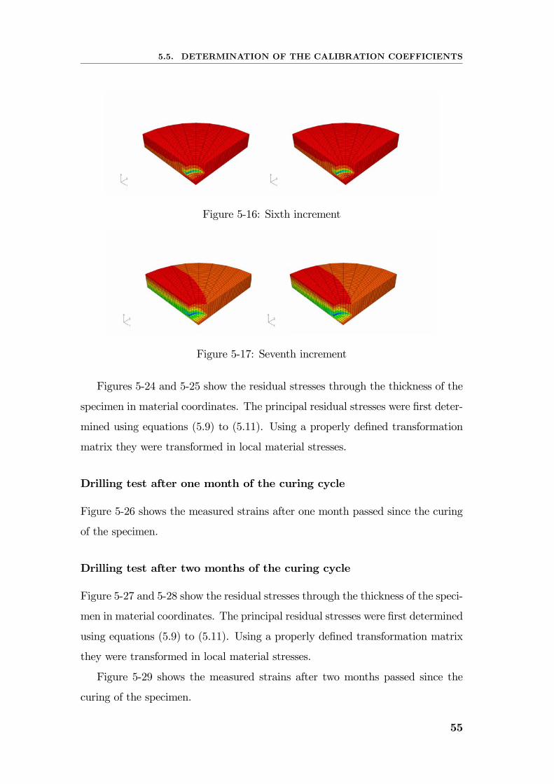
5.5. DETERMINATION OF THE CALIBRATION COEFFICIENTS
Figure 5-16: Sixth increment
Figure 5-17: Seventh increment
Figures 5-24 and 5-25 show the residual stresses through the thickness of the
specimen in material coordinates. The principal residual stresses were first deter-
mined using equations (5.9) to (5.11). Using a properly defined transformation
matrix they were transformed in local material stresses.
Drilling test after one month of the curing cycle
Figure 5-26 shows the measured strains after one month passed since the curing
of the specimen.
Drilling test after two months of the curing cycle
Figure 5-27 and 5-28 show the residual stresses through the thickness of the speci-
men in material coordinates. The principal residual stresses were first determined
using equations (5.9) to (5.11). Using a properly defined transformation matrix
they were transformed in local material stresses.
Figure 5-29 shows the measured strains after two months passed since the
curing of the specimen.
55
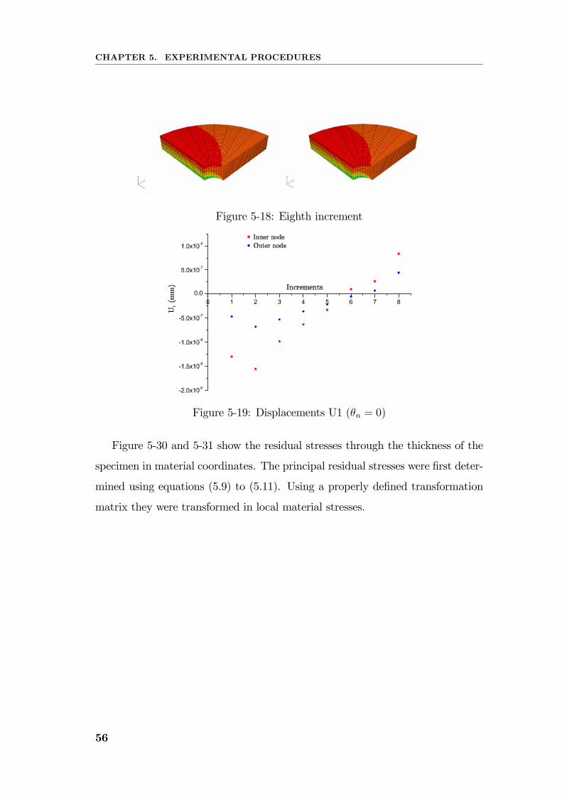
CHAPTER 5. EXPERIMENTAL PROCEDURES
Figure 5-18: Eighth increment
Figure 5-19: Displacements U1 (θn = 0)
Figure 5-30 and 5-31 show the residual stresses through the thickness of the
specimen in material coordinates. The principal residual stresses were first deter-
mined using equations (5.9) to (5.11). Using a properly defined transformation
matrix they were transformed in local material stresses.
56
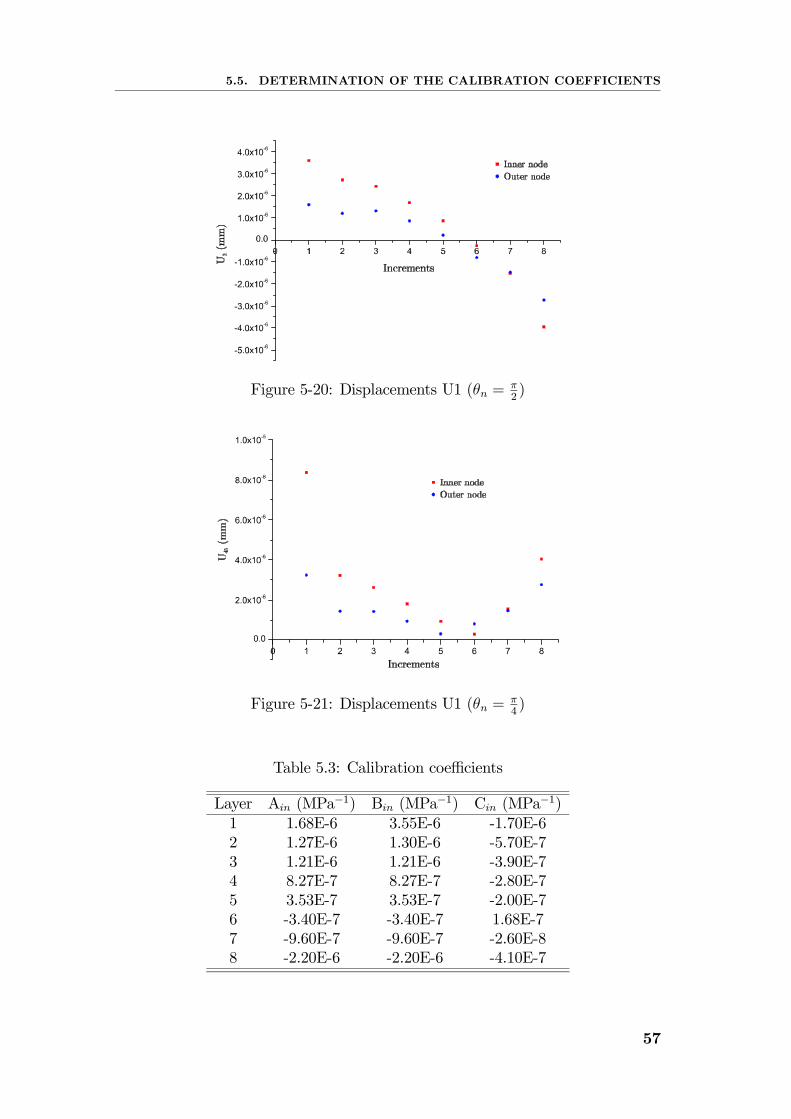
5.5. DETERMINATION OF THE CALIBRATION COEFFICIENTS
Figure 5-20: Displacements U1 (θn = π2)
Figure 5-21: Displacements U1 (θn = π4)
Table 5.3: Calibration coefficients
Layer Ain (MPa−1) Bin (MPa−1) Cin (MPa−1)1 1.68E-6 3.55E-6 -1.70E-62 1.27E-6 1.30E-6 -5.70E-73 1.21E-6 1.21E-6 -3.90E-74 8.27E-7 8.27E-7 -2.80E-75 3.53E-7 3.53E-7 -2.00E-76 -3.40E-7 -3.40E-7 1.68E-77 -9.60E-7 -9.60E-7 -2.60E-88 -2.20E-6 -2.20E-6 -4.10E-7
57
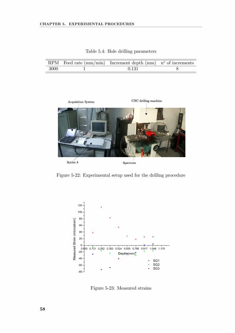
CHAPTER 5. EXPERIMENTAL PROCEDURES
Table 5.4: Hole drilling parameters
RPM Feed rate (mm/min) Increment depth (mm) no of increments3000 1 0.131 8
Figure 5-22: Experimental setup used for the drilling procedure
Figure 5-23: Measured strains
58
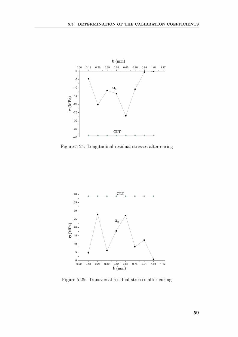
5.5. DETERMINATION OF THE CALIBRATION COEFFICIENTS
Figure 5-24: Longitudinal residual stresses after curing
Figure 5-25: Transversal residual stresses after curing
59
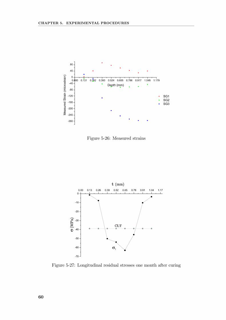
CHAPTER 5. EXPERIMENTAL PROCEDURES
Figure 5-26: Measured strains
Figure 5-27: Longitudinal residual stresses one month after curing
60
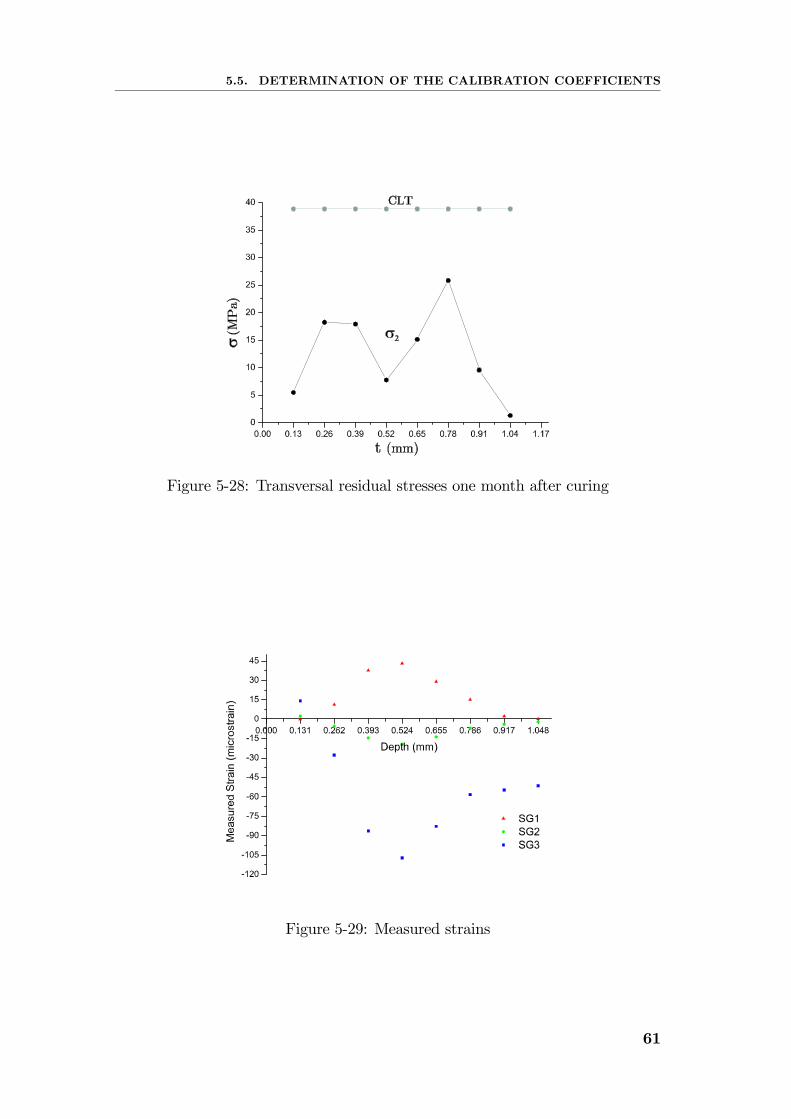
5.5. DETERMINATION OF THE CALIBRATION COEFFICIENTS
Figure 5-28: Transversal residual stresses one month after curing
Figure 5-29: Measured strains
61
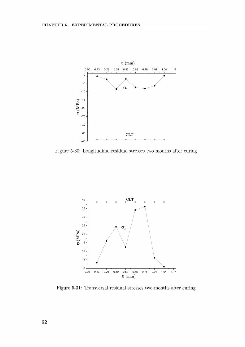
CHAPTER 5. EXPERIMENTAL PROCEDURES
Figure 5-30: Longitudinal residual stresses two months after curing
Figure 5-31: Transversal residual stresses two months after curing
62
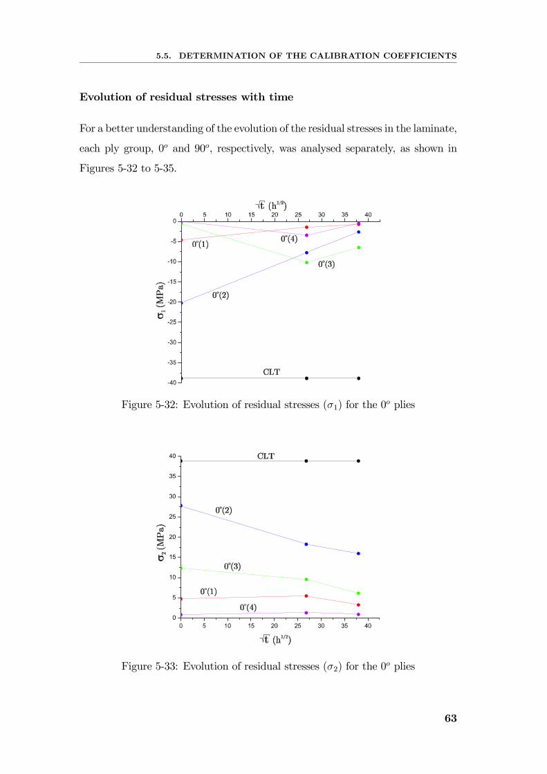
5.5. DETERMINATION OF THE CALIBRATION COEFFICIENTS
Evolution of residual stresses with time
For a better understanding of the evolution of the residual stresses in the laminate,
each ply group, 0o and 90o, respectively, was analysed separately, as shown in
Figures 5-32 to 5-35.
Figure 5-32: Evolution of residual stresses (σ1) for the 0o plies
Figure 5-33: Evolution of residual stresses (σ2) for the 0o plies
63
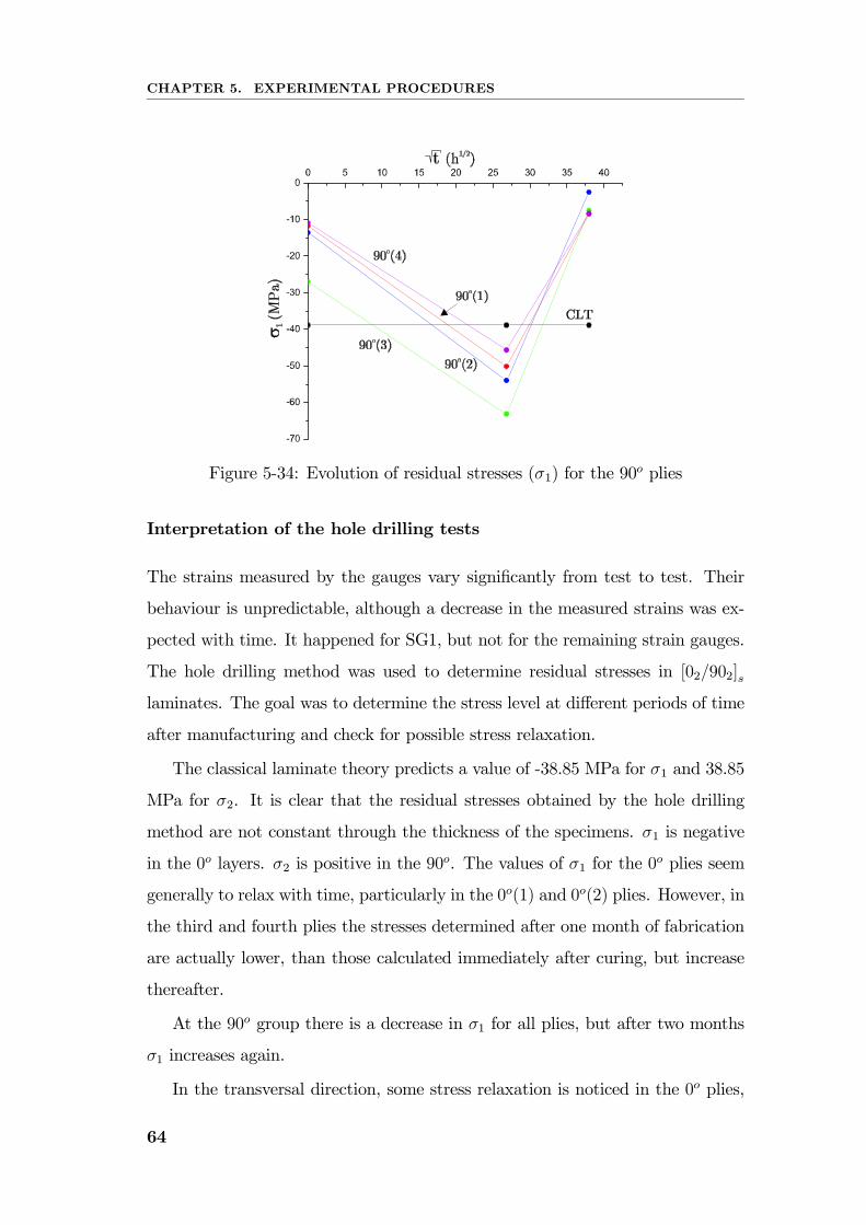
CHAPTER 5. EXPERIMENTAL PROCEDURES
Figure 5-34: Evolution of residual stresses (σ1) for the 90o plies
Interpretation of the hole drilling tests
The strains measured by the gauges vary significantly from test to test. Their
behaviour is unpredictable, although a decrease in the measured strains was ex-
pected with time. It happened for SG1, but not for the remaining strain gauges.
The hole drilling method was used to determine residual stresses in [02/902]s
laminates. The goal was to determine the stress level at different periods of time
after manufacturing and check for possible stress relaxation.
The classical laminate theory predicts a value of -38.85 MPa for σ1 and 38.85
MPa for σ2. It is clear that the residual stresses obtained by the hole drilling
method are not constant through the thickness of the specimens. σ1 is negative
in the 0o layers. σ2 is positive in the 90o. The values of σ1 for the 0o plies seem
generally to relax with time, particularly in the 0o(1) and 0o(2) plies. However, in
the third and fourth plies the stresses determined after one month of fabrication
are actually lower, than those calculated immediately after curing, but increase
thereafter.
At the 90o group there is a decrease in σ1 for all plies, but after two months
σ1 increases again.
In the transversal direction, some stress relaxation is noticed in the 0o plies,
64
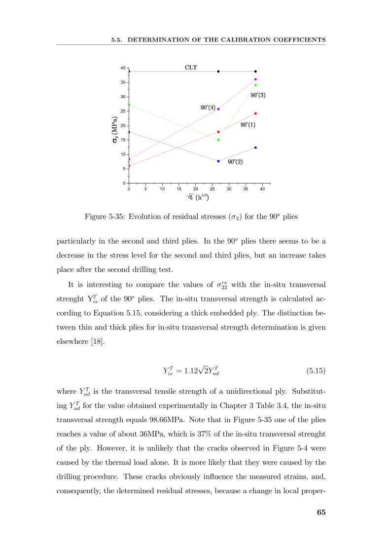
5.5. DETERMINATION OF THE CALIBRATION COEFFICIENTS
Figure 5-35: Evolution of residual stresses (σ2) for the 90o plies
particularly in the second and third plies. In the 90o plies there seems to be a
decrease in the stress level for the second and third plies, but an increase takes
place after the second drilling test.
It is interesting to compare the values of σrs22 with the in-situ transversal
strenght YTis of the 90
o plies. The in-situ transversal strength is calculated ac-
cording to Equation 5.15, considering a thick embedded ply. The distinction be-
tween thin and thick plies for in-situ transversal strength determination is given
elsewhere [18].
Y Tis = 1.12
√2Y T
ud (5.15)
where Y Tud is the transversal tensile strength of a unidirectional ply. Substitut-
ing Y Tud for the value obtained experimentally in Chapter 3 Table 3.4, the in-situ
transversal strength equals 98.66MPa. Note that in Figure 5-35 one of the plies
reaches a value of about 36MPa, which is 37% of the in-situ transversal strenght
of the ply. However, it is unlikely that the cracks observed in Figure 5-4 were
caused by the thermal load alone. It is more likely that they were caused by the
drilling procedure. These cracks obviously influence the measured strains, and,
consequently, the determined residual stresses, because a change in local proper-
65
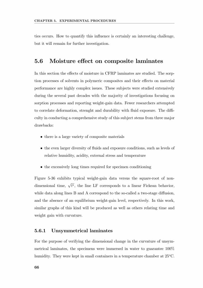
CHAPTER 5. EXPERIMENTAL PROCEDURES
ties occurs. How to quantify this influence is certainly an interesting challenge,
but it will remain for further investigation.
5.6 Moisture effect on composite laminates
In this section the effects of moisture in CFRP laminates are studied. The sorp-
tion processes of solvents in polymeric composites and their effects on material
performance are highly complex issues. These subjects were studied extensively
during the several past decades with the majority of investigations focusing on
sorption processes and reporting weight-gain data. Fewer researchers attempted
to correlate deformation, strenght and durability with fluid exposure. The diffi-
culty in conducting a comprehensive study of this subject stems from three major
drawbacks:
• there is a large variety of composite materials
• the even larger diversity of fluids and exposure conditions, such as levels of
relative humidity, acidity, external stress and temperature
• the excessively long times required for specimen conditioning
Figure 5-36 exhibits typical weight-gain data versus the square-root of non-
dimensional time,√t∗, the line LF corresponds to a linear Fickean behavior,
while data along lines B and A correspond to the so-called a two-stage diffusion,
and the absence of an equilibrium weight-gain level, respectively. In this work,
similar graphs of this kind will be produced as well as others relating time and
weight gain with curvature.
5.6.1 Unsymmetrical laminates
For the purpose of verifying the dimensional change in the curvature of unsym-
metrical laminates, the specimens were immersed in water to guarantee 100%
humidity. They were kept in small containers in a temperature chamber at 25oC.
66
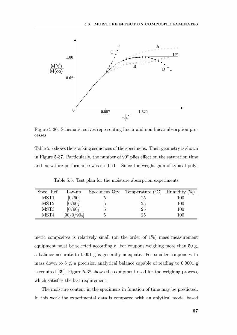
5.6. MOISTURE EFFECT ON COMPOSITE LAMINATES
Figure 5-36: Schematic curves representing linear and non-linear absorption pro-cesses
Table 5.5 shows the stacking sequences of the specimens. Their geometry is shown
in Figure 5-37. Particularly, the number of 90o plies effect on the saturation time
and curvature performance was studied. Since the weight gain of typical poly-
Table 5.5: Test plan for the moisture absorption experiments
Spec. Ref. Lay-up Specimens Qty. Temperature (oC) Humidity (%)MST1 [0/90] 5 25 100MST2 [0/902] 5 25 100MST3 [0/904] 5 25 100MST4 [90/0/903] 5 25 100
meric composites is relatively small (on the order of 1%) mass measurement
equipment must be selected accordingly. For coupons weighing more than 50 g,
a balance accurate to 0.001 g is generally adequate. For smaller coupons with
mass down to 5 g, a precision analytical balance capable of reading to 0.0001 g
is required [39]. Figure 5-38 shows the equipment used for the weighing process,
which satisfies the last requirement.
The moisture content in the specimens in function of time may be predicted.
In this work the experimental data is compared with an anlytical model based
67
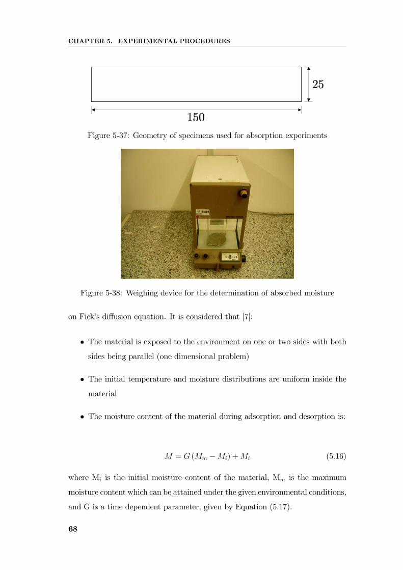
CHAPTER 5. EXPERIMENTAL PROCEDURES
Figure 5-37: Geometry of specimens used for absorption experiments
Figure 5-38: Weighing device for the determination of absorbed moisture
on Fick’s diffusion equation. It is considered that [7]:
• The material is exposed to the environment on one or two sides with both
sides being parallel (one dimensional problem)
• The initial temperature and moisture distributions are uniform inside the
material
• The moisture content of the material during adsorption and desorption is:
M = G (Mm −Mi) +Mi (5.16)
where Mi is the initial moisture content of the material, Mm is the maximum
moisture content which can be attained under the given environmental conditions,
and G is a time dependent parameter, given by Equation (5.17).
68
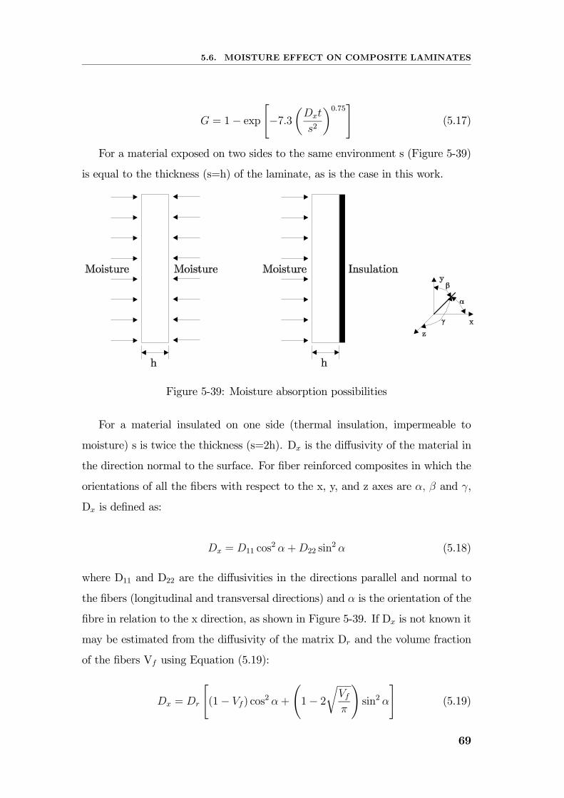
5.6. MOISTURE EFFECT ON COMPOSITE LAMINATES
G = 1− exp"−7.3
µDxt
s2
¶0.75#(5.17)
For a material exposed on two sides to the same environment s (Figure 5-39)
is equal to the thickness (s=h) of the laminate, as is the case in this work.
Figure 5-39: Moisture absorption possibilities
For a material insulated on one side (thermal insulation, impermeable to
moisture) s is twice the thickness (s=2h). Dx is the diffusivity of the material in
the direction normal to the surface. For fiber reinforced composites in which the
orientations of all the fibers with respect to the x, y, and z axes are α, β and γ,
Dx is defined as:
Dx = D11 cos2 α+D22 sin
2 α (5.18)
where D11 and D22 are the diffusivities in the directions parallel and normal to
the fibers (longitudinal and transversal directions) and α is the orientation of the
fibre in relation to the x direction, as shown in Figure 5-39. If Dx is not known it
may be estimated from the diffusivity of the matrix Dr and the volume fraction
of the fibers Vf using Equation (5.19):
Dx = Dr
"(1− Vf) cos
2 α+
Ã1− 2
rVfπ
!sin2 α
#(5.19)
69
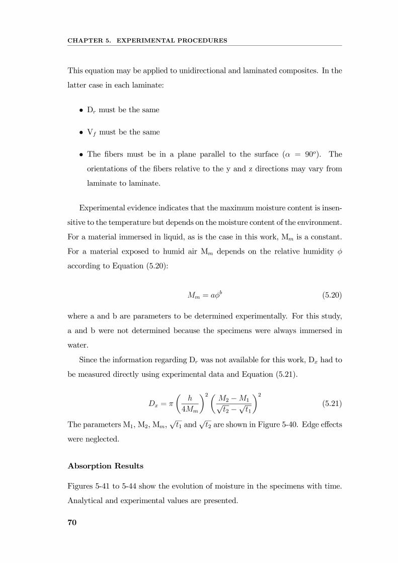
CHAPTER 5. EXPERIMENTAL PROCEDURES
This equation may be applied to unidirectional and laminated composites. In the
latter case in each laminate:
• Dr must be the same
• Vf must be the same
• The fibers must be in a plane parallel to the surface (α = 90o). The
orientations of the fibers relative to the y and z directions may vary from
laminate to laminate.
Experimental evidence indicates that the maximum moisture content is insen-
sitive to the temperature but depends on the moisture content of the environment.
For a material immersed in liquid, as is the case in this work, Mm is a constant.
For a material exposed to humid air Mm depends on the relative humidity φ
according to Equation (5.20):
Mm = aφb (5.20)
where a and b are parameters to be determined experimentally. For this study,
a and b were not determined because the specimens were always immersed in
water.
Since the information regarding Dr was not available for this work, Dx had to
be measured directly using experimental data and Equation (5.21).
Dx = π
µh
4Mm
¶2µM2 −M1√t2 −√t1
¶2(5.21)
The parameters M1, M2, Mm,√t1 and
√t2 are shown in Figure 5-40. Edge effects
were neglected.
Absorption Results
Figures 5-41 to 5-44 show the evolution of moisture in the specimens with time.
Analytical and experimental values are presented.
70
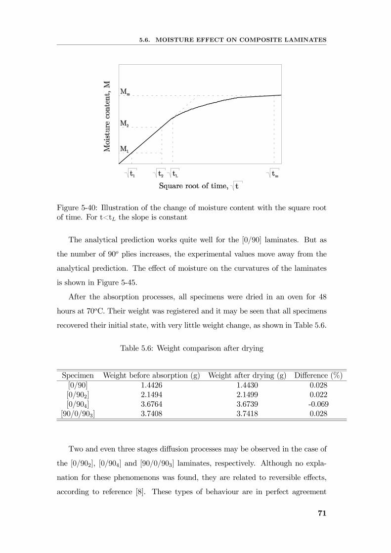
5.6. MOISTURE EFFECT ON COMPOSITE LAMINATES
Figure 5-40: Illustration of the change of moisture content with the square rootof time. For t<tL the slope is constant
The analytical prediction works quite well for the [0/90] laminates. But as
the number of 90o plies increases, the experimental values move away from the
analytical prediction. The effect of moisture on the curvatures of the laminates
is shown in Figure 5-45.
After the absorption processes, all specimens were dried in an oven for 48
hours at 70oC. Their weight was registered and it may be seen that all specimens
recovered their initial state, with very little weight change, as shown in Table 5.6.
Table 5.6: Weight comparison after drying
Specimen Weight before absorption (g) Weight after drying (g) Difference (%)[0/90] 1.4426 1.4430 0.028[0/902] 2.1494 2.1499 0.022[0/904] 3.6764 3.6739 -0.069[90/0/903] 3.7408 3.7418 0.028
Two and even three stages diffusion processes may be observed in the case of
the [0/902], [0/904] and [90/0/903] laminates, respectively. Although no expla-
nation for these phenomenons was found, they are related to reversible effects,
according to reference [8]. These types of behaviour are in perfect agreement
71
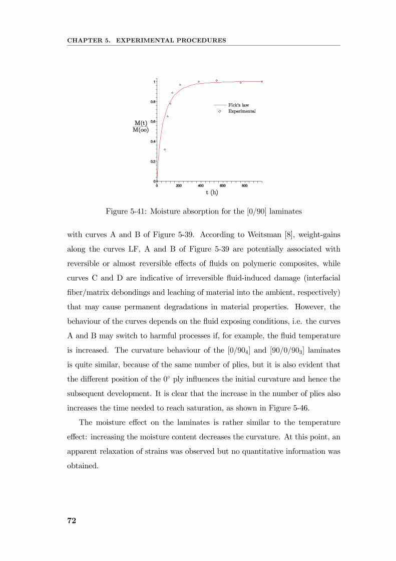
CHAPTER 5. EXPERIMENTAL PROCEDURES
Figure 5-41: Moisture absorption for the [0/90] laminates
with curves A and B of Figure 5-39. According to Weitsman [8], weight-gains
along the curves LF, A and B of Figure 5-39 are potentially associated with
reversible or almost reversible effects of fluids on polymeric composites, while
curves C and D are indicative of irreversible fluid-induced damage (interfacial
fiber/matrix debondings and leaching of material into the ambient, respectively)
that may cause permanent degradations in material properties. However, the
behaviour of the curves depends on the fluid exposing conditions, i.e. the curves
A and B may switch to harmful processes if, for example, the fluid temperature
is increased. The curvature behaviour of the [0/904] and [90/0/903] laminates
is quite similar, because of the same number of plies, but it is also evident that
the different position of the 0 ply influences the initial curvature and hence the
subsequent development. It is clear that the increase in the number of plies also
increases the time needed to reach saturation, as shown in Figure 5-46.
The moisture effect on the laminates is rather similar to the temperature
effect: increasing the moisture content decreases the curvature. At this point, an
apparent relaxation of strains was observed but no quantitative information was
obtained.
72
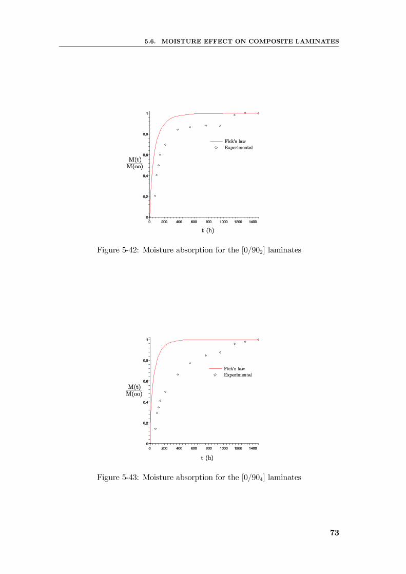
5.6. MOISTURE EFFECT ON COMPOSITE LAMINATES
Figure 5-42: Moisture absorption for the [0/902] laminates
Figure 5-43: Moisture absorption for the [0/904] laminates
73
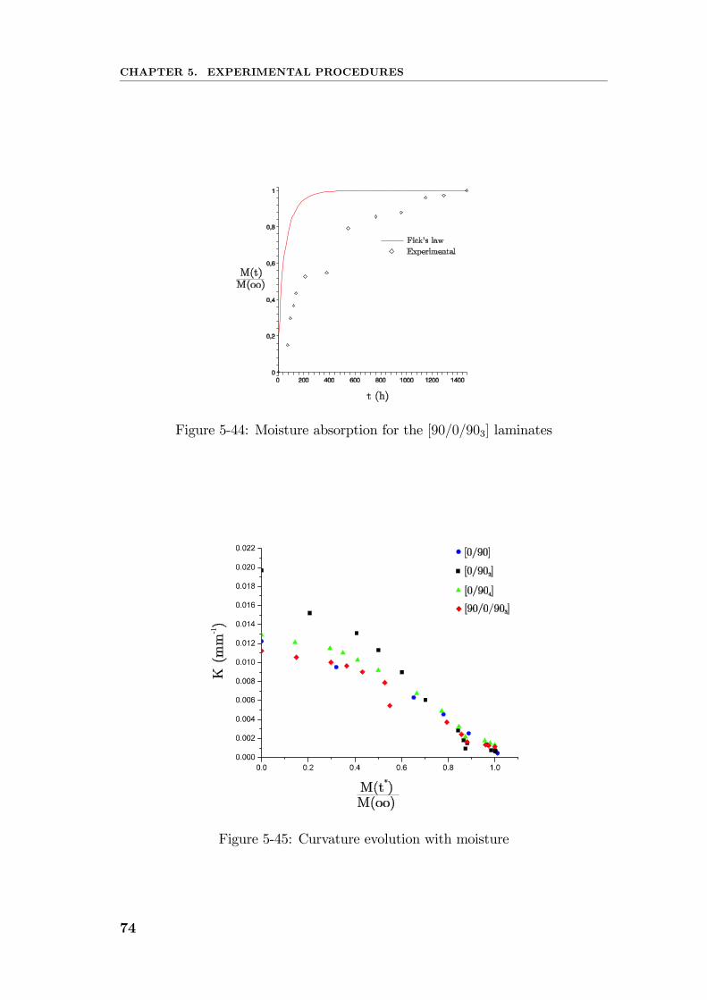
CHAPTER 5. EXPERIMENTAL PROCEDURES
Figure 5-44: Moisture absorption for the [90/0/903] laminates
Figure 5-45: Curvature evolution with moisture
74
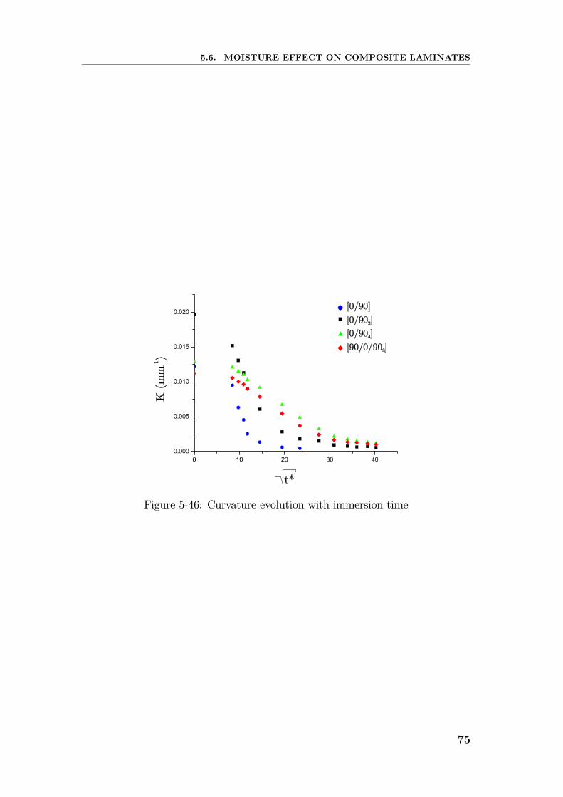
5.6. MOISTURE EFFECT ON COMPOSITE LAMINATES
Figure 5-46: Curvature evolution with immersion time
75

76
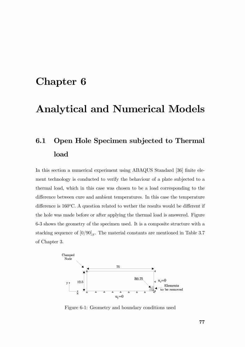
Chapter 6
Analytical and Numerical Models
6.1 Open Hole Specimen subjected to Thermal
load
In this section a numerical experiment using ABAQUS Standard [36] finite ele-
ment technology is conducted to verify the behaviour of a plate subjected to a
thermal load, which in this case was chosen to be a load corresponding to the
difference between cure and ambient temperatures. In this case the temperature
difference is 160oC. A question related to wether the results would be different if
the hole was made before or after applying the thermal load is answered. Figure
6-3 shows the geometry of the specimen used. It is a composite structure with a
stacking sequence of [0/90]S. The material constants are mentioned in Table 3.7
of Chapter 3.
Figure 6-1: Geometry and boundary conditions used
77
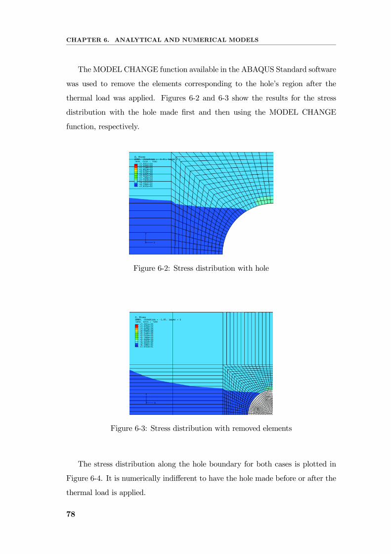
CHAPTER 6. ANALYTICAL AND NUMERICAL MODELS
The MODEL CHANGE function available in the ABAQUS Standard software
was used to remove the elements corresponding to the hole’s region after the
thermal load was applied. Figures 6-2 and 6-3 show the results for the stress
distribution with the hole made first and then using the MODEL CHANGE
function, respectively.
Figure 6-2: Stress distribution with hole
Figure 6-3: Stress distribution with removed elements
The stress distribution along the hole boundary for both cases is plotted in
Figure 6-4. It is numerically indifferent to have the hole made before or after the
thermal load is applied.
78
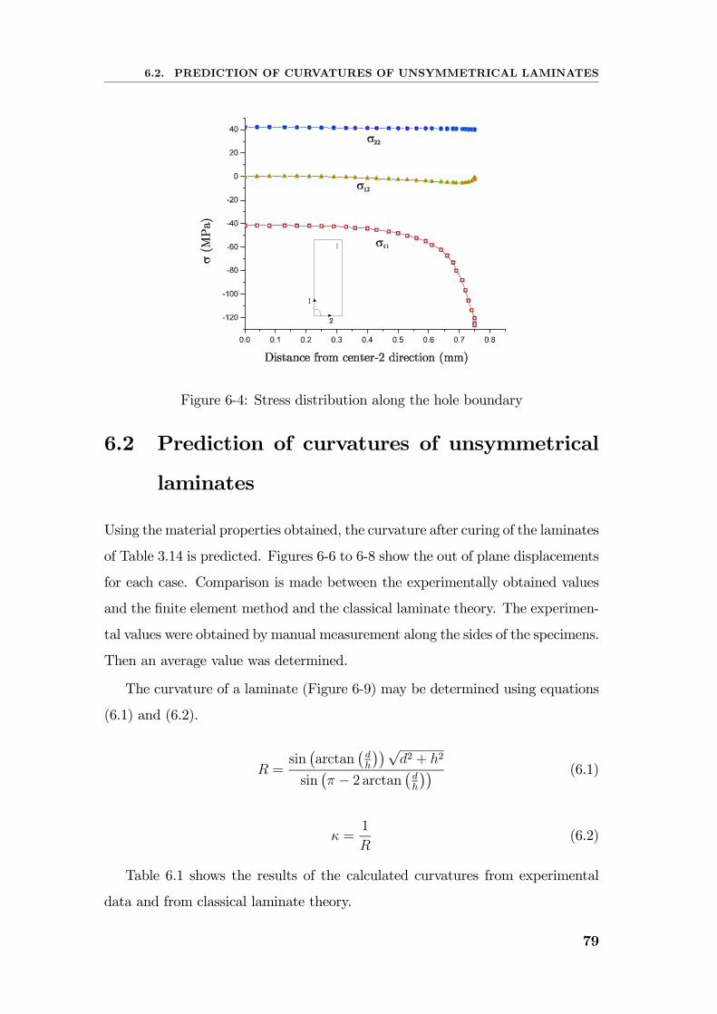
6.2. PREDICTION OF CURVATURES OF UNSYMMETRICAL LAMINATES
Figure 6-4: Stress distribution along the hole boundary
6.2 Prediction of curvatures of unsymmetrical
laminates
Using the material properties obtained, the curvature after curing of the laminates
of Table 3.14 is predicted. Figures 6-6 to 6-8 show the out of plane displacements
for each case. Comparison is made between the experimentally obtained values
and the finite element method and the classical laminate theory. The experimen-
tal values were obtained by manual measurement along the sides of the specimens.
Then an average value was determined.
The curvature of a laminate (Figure 6-9) may be determined using equations
(6.1) and (6.2).
R =sin¡arctan
¡dh
¢¢√d2 + h2
sin¡π − 2 arctan
¡dh
¢¢ (6.1)
κ =1
R(6.2)
Table 6.1 shows the results of the calculated curvatures from experimental
data and from classical laminate theory.
79
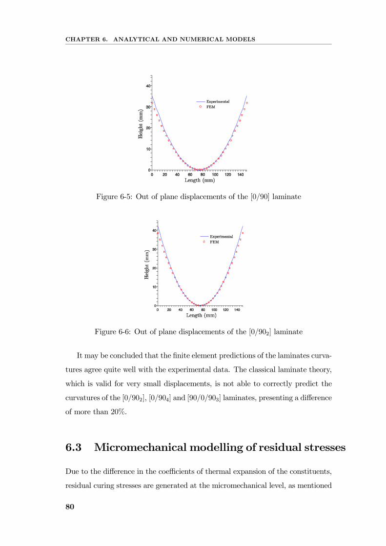
CHAPTER 6. ANALYTICAL AND NUMERICAL MODELS
Figure 6-5: Out of plane displacements of the [0/90] laminate
Figure 6-6: Out of plane displacements of the [0/902] laminate
It may be concluded that the finite element predictions of the laminates curva-
tures agree quite well with the experimental data. The classical laminate theory,
which is valid for very small displacements, is not able to correctly predict the
curvatures of the [0/902], [0/904] and [90/0/903] laminates, presenting a difference
of more than 20%.
6.3 Micromechanical modelling of residual stresses
Due to the difference in the coefficients of thermal expansion of the constituents,
residual curing stresses are generated at the micromechanical level, as mentioned
80
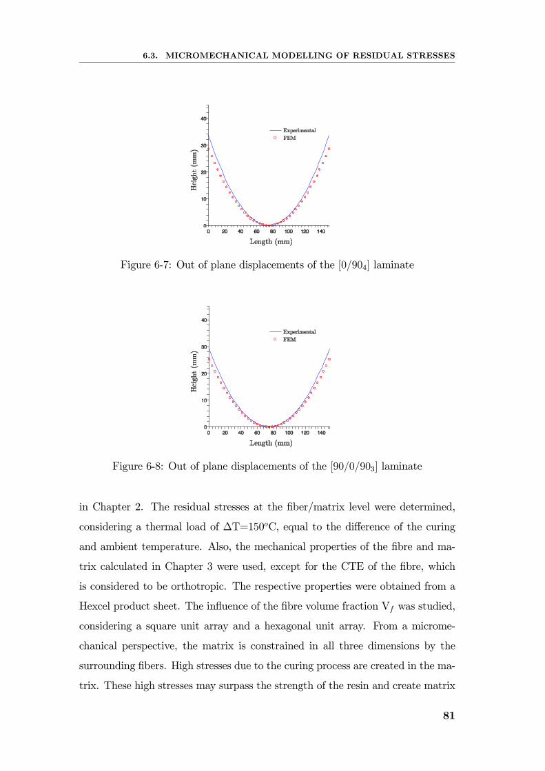
6.3. MICROMECHANICAL MODELLING OF RESIDUAL STRESSES
Figure 6-7: Out of plane displacements of the [0/904] laminate
Figure 6-8: Out of plane displacements of the [90/0/903] laminate
in Chapter 2. The residual stresses at the fiber/matrix level were determined,
considering a thermal load of ∆T=150oC, equal to the difference of the curing
and ambient temperature. Also, the mechanical properties of the fibre and ma-
trix calculated in Chapter 3 were used, except for the CTE of the fibre, which
is considered to be orthotropic. The respective properties were obtained from a
Hexcel product sheet. The influence of the fibre volume fraction Vf was studied,
considering a square unit array and a hexagonal unit array. From a microme-
chanical perspective, the matrix is constrained in all three dimensions by the
surrounding fibers. High stresses due to the curing process are created in the ma-
trix. These high stresses may surpass the strength of the resin and create matrix
81
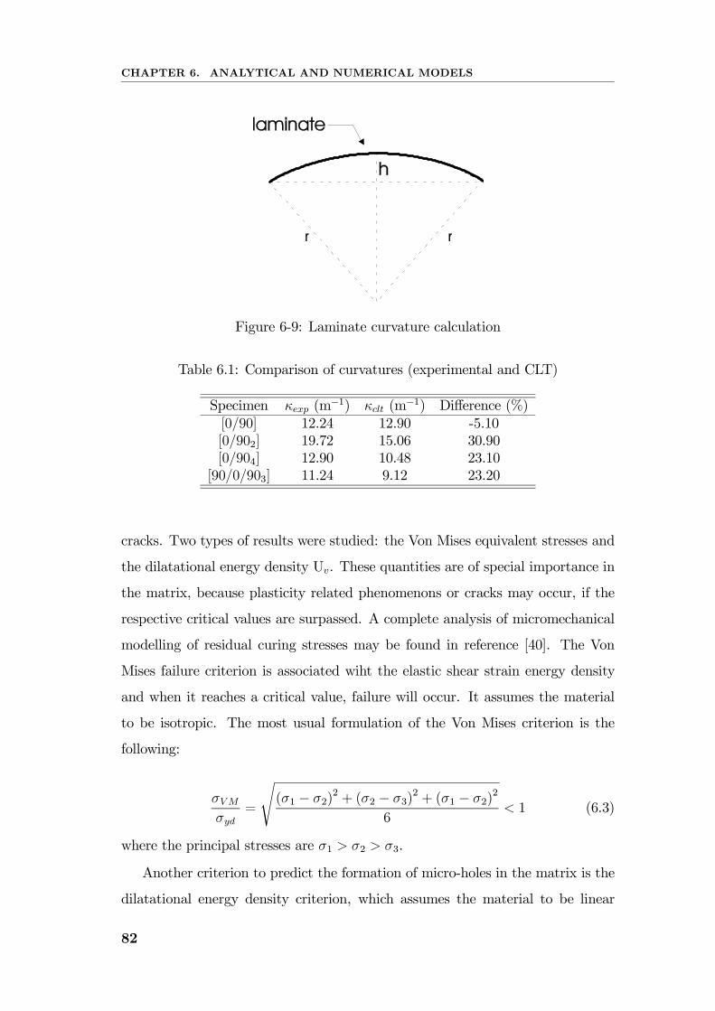
CHAPTER 6. ANALYTICAL AND NUMERICAL MODELS
Figure 6-9: Laminate curvature calculation
Table 6.1: Comparison of curvatures (experimental and CLT)
Specimen κexp (m−1) κclt (m−1) Difference (%)[0/90] 12.24 12.90 -5.10[0/902] 19.72 15.06 30.90[0/904] 12.90 10.48 23.10[90/0/903] 11.24 9.12 23.20
cracks. Two types of results were studied: the Von Mises equivalent stresses and
the dilatational energy density Uv. These quantities are of special importance in
the matrix, because plasticity related phenomenons or cracks may occur, if the
respective critical values are surpassed. A complete analysis of micromechanical
modelling of residual curing stresses may be found in reference [40]. The Von
Mises failure criterion is associated wiht the elastic shear strain energy density
and when it reaches a critical value, failure will occur. It assumes the material
to be isotropic. The most usual formulation of the Von Mises criterion is the
following:
σVMσyd
=
s(σ1 − σ2)
2 + (σ2 − σ3)2 + (σ1 − σ2)
2
6< 1 (6.3)
where the principal stresses are σ1 > σ2 > σ3.
Another criterion to predict the formation of micro-holes in the matrix is the
dilatational energy density criterion, which assumes the material to be linear
82
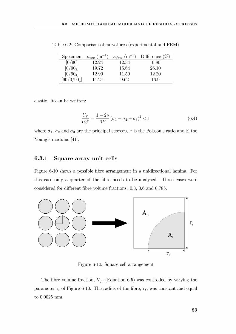
6.3. MICROMECHANICAL MODELLING OF RESIDUAL STRESSES
Table 6.2: Comparison of curvatures (experimental and FEM)
Specimen κexp (m−1) κfem (m−1) Difference (%)[0/90] 12.24 12.34 -0.80[0/902] 19.72 15.64 26.10[0/904] 12.90 11.50 12.20[90/0/903] 11.24 9.62 16.9
elastic. It can be written:
UV
U crV
=1− 2ν6E
(σ1 + σ2 + σ3)2 < 1 (6.4)
where σ1, σ2 and σ3 are the principal stresses, ν is the Poisson’s ratio and E the
Young’s modulus [41].
6.3.1 Square array unit cells
Figure 6-10 shows a possible fibre arrangement in a unidirectional lamina. For
this case only a quarter of the fibre needs to be analysed. Three cases were
considered for different fibre volume fractions: 0.3, 0.6 and 0.785.
Figure 6-10: Square cell arrangement
The fibre volume fraction, Vf , (Equation 6.5) was controlled by varying the
parameter rt of Figure 6-10. The radius of the fibre, rf , was constant and equal
to 0.0025 mm.
83
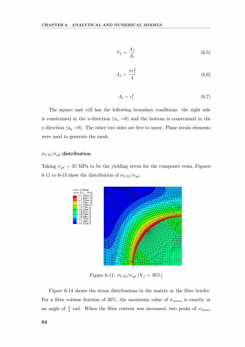
CHAPTER 6. ANALYTICAL AND NUMERICAL MODELS
Vf =Af
At(6.5)
Af =πr2f4
(6.6)
At = r2t (6.7)
The square unit cell has the following boundary conditions: the right side
is constrained in the x-direction (ux =0) and the bottom is constrained in the
y-direction (uy =0). The other two sides are free to move. Plane strain elements
were used to generate the mesh.
σVM/σyd distribution
Taking σyd = 35 MPa to be the yielding stress for the composite resin, Figures
6-11 to 6-13 show the distribution of σVM/σyd.
Figure 6-11: σVM/σyd (Vf = 30%)
Figure 6-14 shows the stress distributions in the matrix at the fibre border.
For a fibre volume fraction of 30%, the maximum value of σmises is exactly at
an angle of π4rad. When the fibre content was increased, two peaks of σmises
84
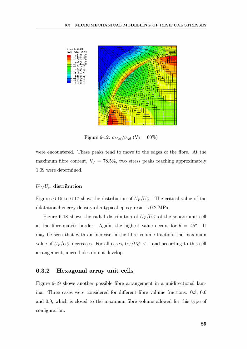
6.3. MICROMECHANICAL MODELLING OF RESIDUAL STRESSES
Figure 6-12: σVM/σyd (Vf = 60%)
were encountered. These peaks tend to move to the edges of the fibre. At the
maximum fibre content, Vf = 78.5%, two stress peaks reaching approximately
1.09 were determined.
UV /Ucr distribution
Figures 6-15 to 6-17 show the distribution of UV /UcrV . The critical value of the
dilatational energy density of a typical epoxy resin is 0.2 MPa.
Figure 6-18 shows the radial distribution of UV /UcrV of the square unit cell
at the fibre-matrix border. Again, the highest value occurs for θ = 45o. It
may be seen that with an increase in the fibre volume fraction, the maximum
value of UV /UcrV decreases. For all cases, UV /U
crV < 1 and according to this cell
arrangement, micro-holes do not develop.
6.3.2 Hexagonal array unit cells
Figure 6-19 shows another possible fibre arrangement in a unidirectional lam-
ina. Three cases were considered for different fibre volume fractions: 0.3, 0.6
and 0.9, which is closed to the maximum fibre volume allowed for this type of
configuration.
85
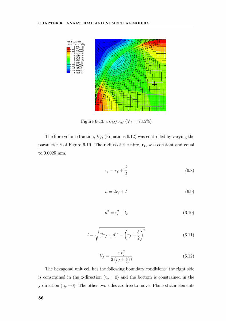
CHAPTER 6. ANALYTICAL AND NUMERICAL MODELS
Figure 6-13: σVM/σyd (Vf = 78.5%)
The fibre volume fraction, Vf , (Equations 6.12) was controlled by varying the
parameter δ of Figure 6-19. The radius of the fibre, rf , was constant and equal
to 0.0025 mm.
rt = rf +δ
2(6.8)
h = 2rf + δ (6.9)
h2 = r2t + l2 (6.10)
l =
s(2rf + δ)2 −
µrf +
δ
2
¶2(6.11)
Vf =πr2f
2¡rf +
δ2
¢l
(6.12)
The hexagonal unit cell has the following boundary conditions: the right side
is constrained in the x-direction (ux =0) and the bottom is constrained in the
y-direction (uy =0). The other two sides are free to move. Plane strain elements
86
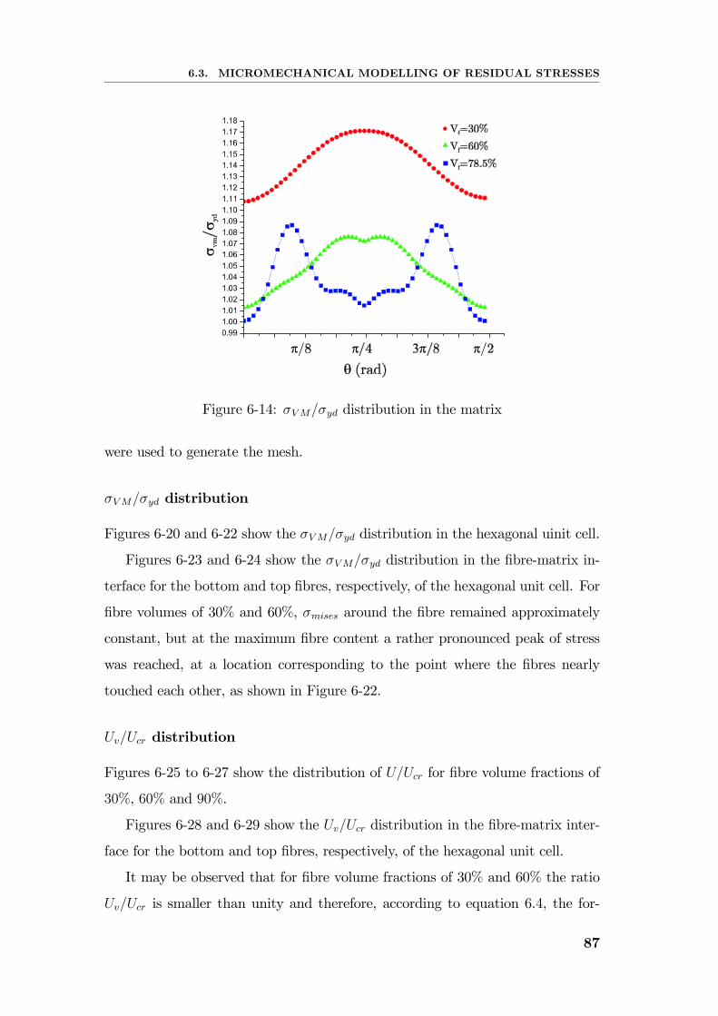
6.3. MICROMECHANICAL MODELLING OF RESIDUAL STRESSES
Figure 6-14: σVM/σyd distribution in the matrix
were used to generate the mesh.
σVM/σyd distribution
Figures 6-20 and 6-22 show the σVM/σyd distribution in the hexagonal uinit cell.
Figures 6-23 and 6-24 show the σVM/σyd distribution in the fibre-matrix in-
terface for the bottom and top fibres, respectively, of the hexagonal unit cell. For
fibre volumes of 30% and 60%, σmises around the fibre remained approximately
constant, but at the maximum fibre content a rather pronounced peak of stress
was reached, at a location corresponding to the point where the fibres nearly
touched each other, as shown in Figure 6-22.
Uv/Ucr distribution
Figures 6-25 to 6-27 show the distribution of U/Ucr for fibre volume fractions of
30%, 60% and 90%.
Figures 6-28 and 6-29 show the Uv/Ucr distribution in the fibre-matrix inter-
face for the bottom and top fibres, respectively, of the hexagonal unit cell.
It may be observed that for fibre volume fractions of 30% and 60% the ratio
Uv/Ucr is smaller than unity and therefore, according to equation 6.4, the for-
87
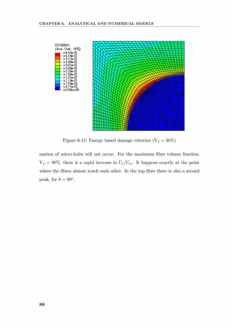
CHAPTER 6. ANALYTICAL AND NUMERICAL MODELS
Figure 6-15: Energy based damage criterion (Vf = 30%)
mation of micro-holes will not occur. For the maximum fibre volume fraction,
Vf = 90%, there is a rapid increase in Uv/Ucr. It happens exactly at the point
where the fibres almost touch each other. In the top fibre there is also a second
peak, for θ = 90o.
88
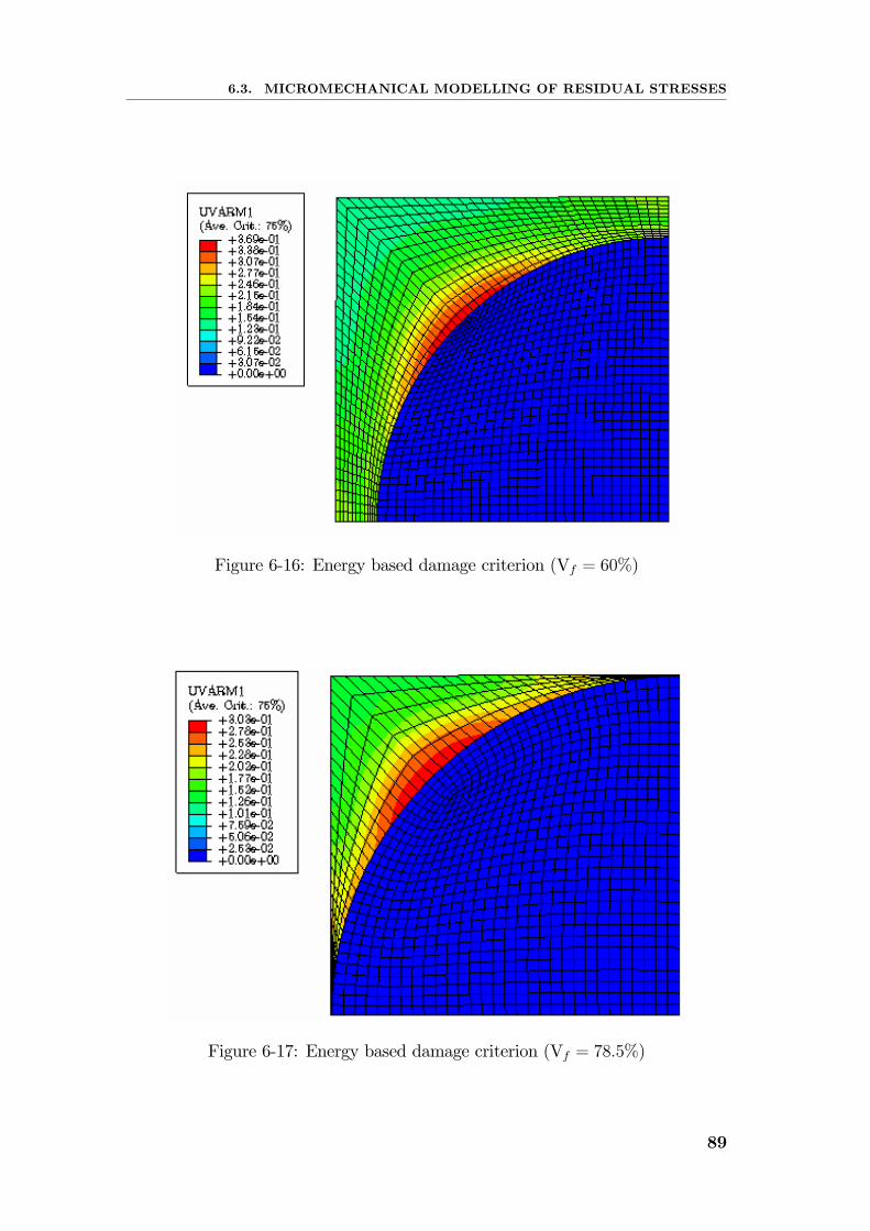
6.3. MICROMECHANICAL MODELLING OF RESIDUAL STRESSES
Figure 6-16: Energy based damage criterion (Vf = 60%)
Figure 6-17: Energy based damage criterion (Vf = 78.5%)
89
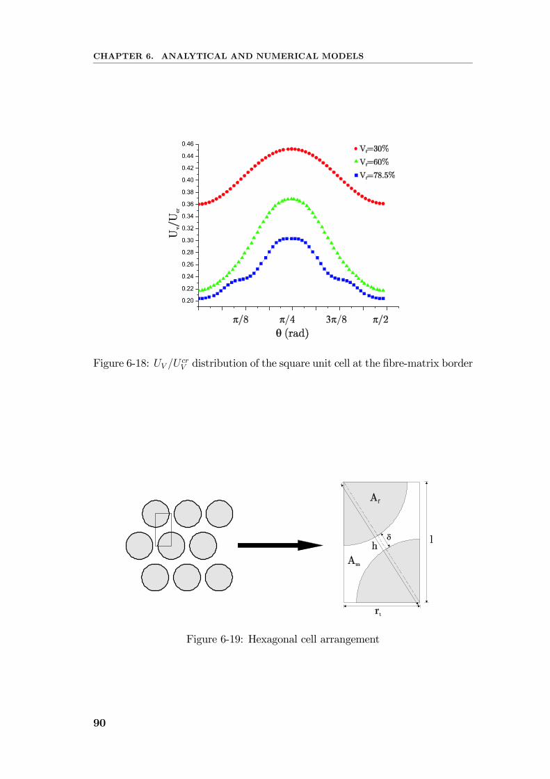
CHAPTER 6. ANALYTICAL AND NUMERICAL MODELS
Figure 6-18: UV /UcrV distribution of the square unit cell at the fibre-matrix border
Figure 6-19: Hexagonal cell arrangement
90
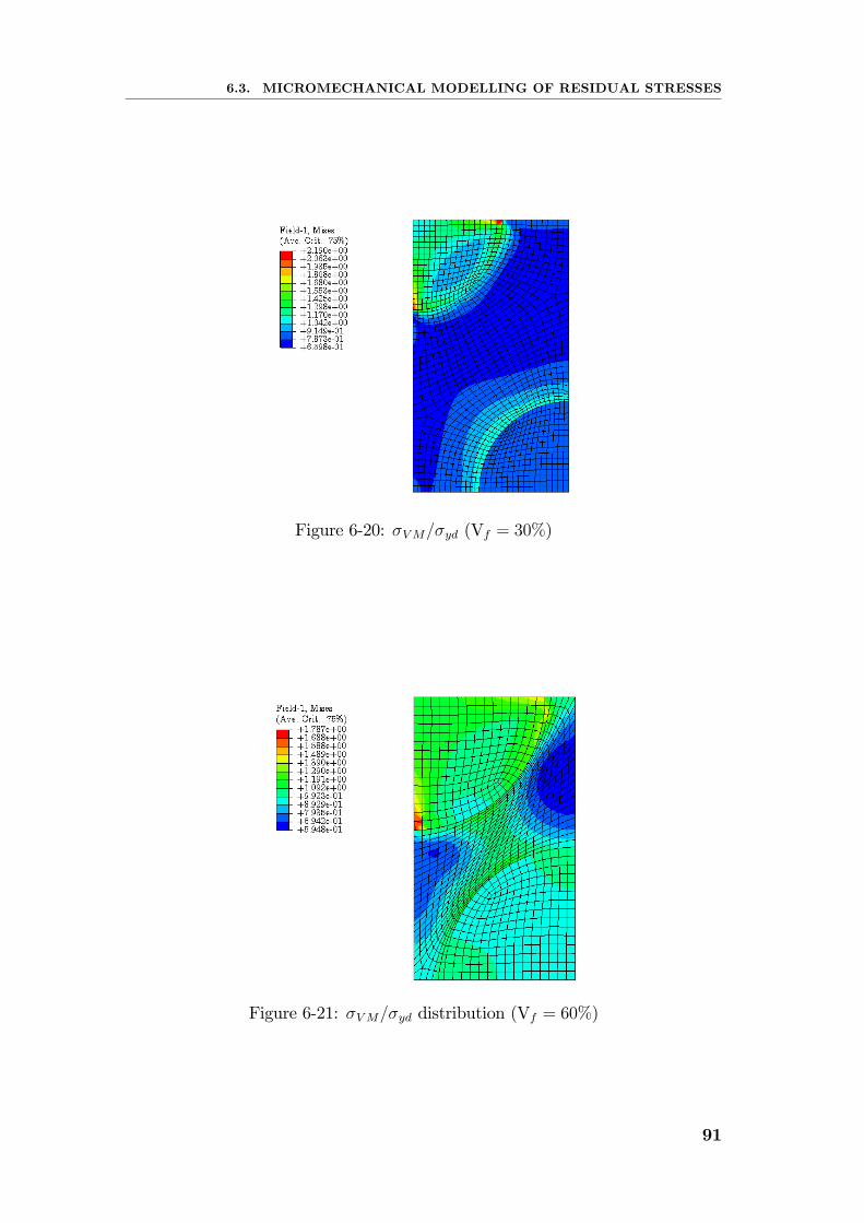
6.3. MICROMECHANICAL MODELLING OF RESIDUAL STRESSES
Figure 6-20: σVM/σyd (Vf = 30%)
Figure 6-21: σVM/σyd distribution (Vf = 60%)
91
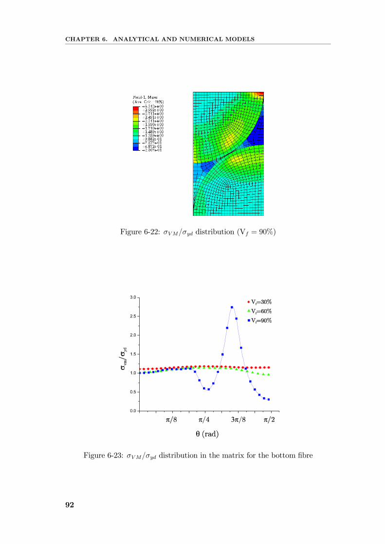
CHAPTER 6. ANALYTICAL AND NUMERICAL MODELS
Figure 6-22: σVM/σyd distribution (Vf = 90%)
Figure 6-23: σVM/σyd distribution in the matrix for the bottom fibre
92
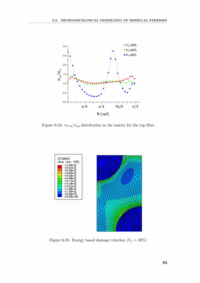
6.3. MICROMECHANICAL MODELLING OF RESIDUAL STRESSES
Figure 6-24: σVM/σyd distribution in the matrix for the top fibre
Figure 6-25: Energy based damage criterion (Vf = 30%)
93
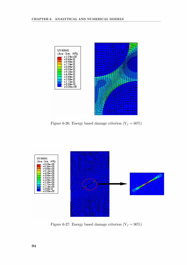
CHAPTER 6. ANALYTICAL AND NUMERICAL MODELS
Figure 6-26: Energy based damage criterion (Vf = 60%)
Figure 6-27: Energy based damage criterion (Vf = 90%)
94
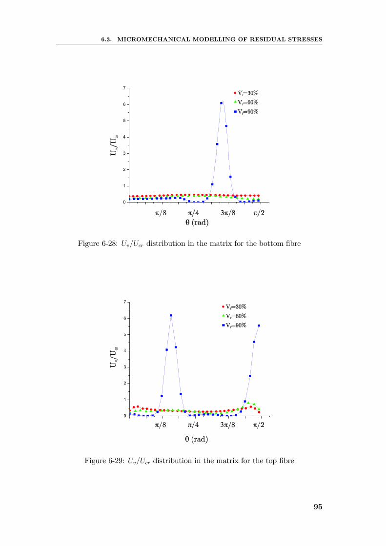
6.3. MICROMECHANICAL MODELLING OF RESIDUAL STRESSES
Figure 6-28: Uv/Ucr distribution in the matrix for the bottom fibre
Figure 6-29: Uv/Ucr distribution in the matrix for the top fibre
95

96
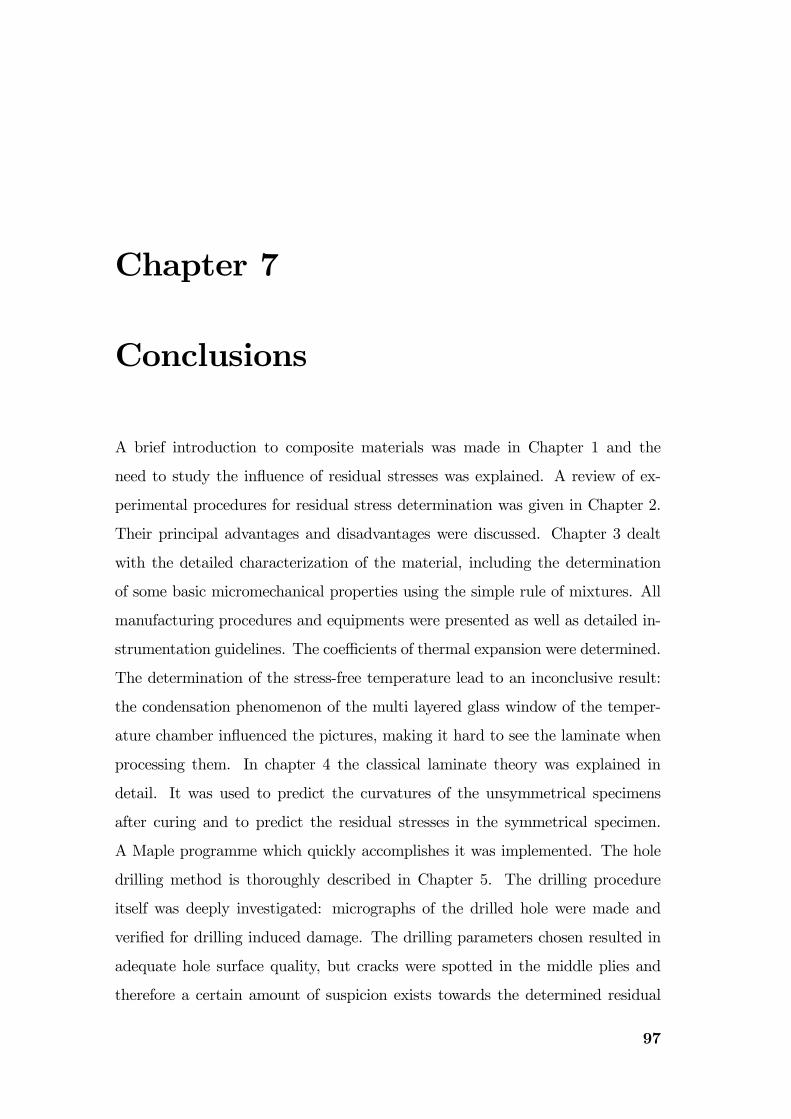
Chapter 7
Conclusions
A brief introduction to composite materials was made in Chapter 1 and the
need to study the influence of residual stresses was explained. A review of ex-
perimental procedures for residual stress determination was given in Chapter 2.
Their principal advantages and disadvantages were discussed. Chapter 3 dealt
with the detailed characterization of the material, including the determination
of some basic micromechanical properties using the simple rule of mixtures. All
manufacturing procedures and equipments were presented as well as detailed in-
strumentation guidelines. The coefficients of thermal expansion were determined.
The determination of the stress-free temperature lead to an inconclusive result:
the condensation phenomenon of the multi layered glass window of the temper-
ature chamber influenced the pictures, making it hard to see the laminate when
processing them. In chapter 4 the classical laminate theory was explained in
detail. It was used to predict the curvatures of the unsymmetrical specimens
after curing and to predict the residual stresses in the symmetrical specimen.
A Maple programme which quickly accomplishes it was implemented. The hole
drilling method is thoroughly described in Chapter 5. The drilling procedure
itself was deeply investigated: micrographs of the drilled hole were made and
verified for drilling induced damage. The drilling parameters chosen resulted in
adequate hole surface quality, but cracks were spotted in the middle plies and
therefore a certain amount of suspicion exists towards the determined residual
97
CHAPTER 7. CONCLUSIONS
stresses. When comparing the residual stresses obtained through the hole drilling
method with the values predicted by the classical laminate theory, it is apparent
that the residual stresses are not constant through the thickness of the specimen.
An apparent relaxation of the stresses seems to take place with time, but it was
impossible to quantify it at the actual position of this work, because this phe-
nomenon did not happen in all plies in a coherent manner. Also, the presence of
the cracks may contribute to an apparent stress relaxation, because local material
properties are diminished. The values of σ2 corresponding to the 90o plies were
compared to the in-situ transversal strength of the plies. It was concluded that
the residual stress level may reach about 37% of the in-situ transversal strength
of the ply, but it is not thought to be the cause of the cracks. The moisture
effect on unsymmetrical laminates was studied. In this work several laminates
with stacking sequences of [0/90], [0/902], [0/904] and [90/0/903] were immersed
in water and their absorption behaviour and curvature were investigated. An
almost perfect fit using Fick’s equation was obtained for the [0/90] laminate, but
for the remaining laminates the experimental data departed the linear Fickian
behaviour. This subject will require furhter investigation. The curvature of the
laminates decreased in an almost linear way with moisture increase. The increase
in number of plies contributes to an increase in saturation time. In Chapter 6,
a numerical experiment of a plate containing a hole was performed. The stress
distribution along the hole boundary was determined and the results are the same
if the elements are removed after or before the application of the thermal load.
The finite element method was also used to predict the curvature of the cured
unsymmetrical laminates. The experimental values agreed well with the finite el-
ement method predictions. On the other hand, the classical laminate theory was
not able to predict the curvatures in a satisfactory manner. The determination
of residual stresses at the micromechanical level, i.e. between fibres and matrix,
using the properties determined in Chapter 3 was made. It was concluded that
matrix cracks may develop, particularly at high fibre volume fractions. For fu-
ture developments, it would be necessary to characterize the development of the
98
resin properties with time and temperature for a better modelling of microme-
chanical thermally induced residual stresses. Further experiments using the hole
drilling method should be conducted using more increments per ply to explore
the sensitivity of the method. It is important to mention the fact that some im-
portant progress has been accomplished, specially the walls of the hole due to the
drilling process and the detailed material characterization. However, the presence
of cracks in drilled specimens should be the subject of further investigation. For
this purpose, several stacking sequences should be tested. Combining this with
different composite materials should prove to be a challenging work. Without an
excellent hole quality, the application of the hole drilling method in composite
laminates will not advance. A programme which optimizes the determination of
the calibration constants in function of hole geometry and laminate characteris-
tics could be an interesting development, to facilitate the determination of the
residual stresses. The relaxation of stresses is an interesting and complex subject
but should consist in a potential objective for further exploration.
99

100
Bibliography
[1] Ori Ishai Isaac M. Daniel. Engineering Mechanics of Composite Materials.
Oxford University Press, 1994.
[2] William F. Smith. Principles of Materials Science and Engineering.
McGraw-Hill, Inc., 1996.
[3] Robert M. Jones. Mechanics of Composite Materials. Taylor Francis, Inc,
1999.
[4] H. Thomas Hahn Stephen W. Tsai. Introduction to Composite Materials.
Technomic Publishing Company, 1980.
[5] Won J. Yu Paul Sunderland and Jan-Anders E. Manson. A technique for the
measurement of process-induced internal stresses in polymers and polymer
composites". ICCM 10, pages 125—132, 1995.
[6] ASTM International. Standard test method for determining residual stresses
by the hole-drilling strain gage method (e 837-01). Technical report, Novem-
ber 2001.
[7] George S. Springer. Environmental Effects on Composite Materials. Tech-
nomic Publishing Company, Inc, 1981.
[8] M. Elahi Y.J. Weitsman. Effects of fluids on the deformation, strength
and durability of polymeric composites- an overview. Mechanics of Time-
Dependent Materials, pages 107—126, 2000.
101
BIBLIOGRAPHY
[9] B. Fiedler et Al. The influence of thermal residual stresses on the transverse
strength of cfrp using fem. Composites: Part A, 33:1323—1326.
[10] Göran Fernlund et Al. Residual stress, spring in and warpage in autoclaved
composite parts. ICCM 14, pages 1—10, 2003.
[11] K.D. Potter M. Gigliotti, M.R. Wisnom. Development of curvature during
the cure of AS4/8552 [0/90] unsymmetric composite plates. Composites
Science and Technology, 63:187—197, 2003.
[12] Gong X.Lu et al. Residual stress distribution and its influence on the me-
chanical behaviour of composite laminates. ICCM 12, 1999.
[13] L.G.Stringer et Al. Curing stresses in thick polymer composite components;
part II: Management of residual stresses.
[14] J.A. Nairn. Fracture mechanics of composites with residual stresses, traction-
loaded cracks and imperfect interfaces. Proc. 2nd ESIS TC4 Conference on
Polymers and Composites, in press, 1999.
[15] José Joaquim Lopes Morais. Influência Do Meio Ambiente No Compor-
tamento Ao Dano de Estruturas Em Materiais Compósitos. PhD thesis,
Universidade de Trás os Montes e Alto Douro, 1998.
[16] P.K. Predecki et al B. Benedikt, M. Kumosa. An analysis of residual ther-
mal stresses in a unidirectional graphite/PMR-15 composite based on x-
ray diffraction measurements. Composites Science and Technology, 61:1977—
1994, 2001.
[17] Peter W. R. Beaumont Kevin D. Cowley. The measurement and prediction
of residual stresses in carbon-fibre/polymer composites. Composite Science
and Technology, 57:1445—1455, 1997.
[18] Pedro Camanho et Al. Failure models and criteria for FRP under in-plane
or three-dimensional stress states including shear non-linearity. Technical
report, NASA, 2005.
102
BIBLIOGRAPHY
[19] A. Turnbull et Al. Residual stress in polymers: Evaluation of measurement
techniques. Journal of Materials Science, 34:451—459, 1999.
[20] Maria Teresa Restivo Jorge Borges de Almeida, António Torres Marques.
Utilização do método do furo para a determinação de tensões residuais em
materiais poliméricos. In 3z Congresso Luso-Moçambicano de Engenharia,
2003.
[21] Jorge Borges de Almeida. Determination of residual stresses in CFRP lam-
inates using the hole drilling method. Technical report, FEUP, June 2004.
[22] O. Sicot et al. Determination of residual stress in composite laminates us-
ing the incremental hole-drilling method". Journal of Composite Materials,
37:831—814, 2003.
[23] H. T. Hahn S. R. White. Process modeling of composite materials: Resid-
ual stress development during cure. part i. model formulation. Journal of
Composite Materials, 26(16):2402—2422, 1992.
[24] ASTM. Standard test method for tensile properties of polymer matrix com-
posite materials ASTM d 3039/d 3039m.00. Technical report, American
Society for Testing and Materials (ASTM).
[25] ASTM. Standard test method for in-plane shear response of polymer matrix
compos- ite materials by test of a g45o laminate, ASTM d 3518/3518m-94.
Technical report, American Society for Testing and Materials (ASTM).
[26] Leif A. Carlsson R. Byron Pipes. Experimental Characterization of Advanced
Composite Materials. Technomic Publishing Co. Inc., 1997.
[27] J.D.D. Melo D.W. Radford. Elastic characterization of PEEK/IM7 using
coefficients of thermal expansion. Composites: Part A, 33:1505—1510, 2002.
[28] Murat H. Kural Donald L. Flaggs. Experimental determination of the in
situ transverse lamina strength in graphite/epoxy laminates. Journal of
Composite Materials, 16:103—114, 1982.
103
BIBLIOGRAPHY
[29] Adrian Biran and Moshe Breiner. Matlab 6 for Engineers. Pearson Educa-
tion, 2002.
[30] Waterloo Maple Inc. Canada. Maple 9.5 Users Manual, 2002.
[31] Componeering. Esacomp 2.1 User’s Manual, 2000.
[32] W. Soete. Measurement and relaxation of residual stress. Sheet Met Ind,
26:1269—1281, 1949.
[33] B. R. Lake et Al. A method for measuring planar residual stresses in rect-
angular orthotropic materials. Journal of Composite Materials, 2:244—253,
1968.
[34] C. K. H. Dharan H. Ho-Cheng. Delamination during drilling in composite
laminates. American Society Mechanical Engineers, 112:236—239, 1990.
[35] C. Würtz F. Klocke. The use of pcd tools for machining fibre reinforced
materials. European Conference Composite Materials 8, pages 509—515, 2002.
[36] Karlsson Hibbitt and Sorensen. Abaqus 6.4 User’s Manuals, 2003.
[37] Maria Odete Rodrigues Cadete. A Linguagem Fortran 77. Fundação
Calouste Gulbenkian, 1997.
[38] O. Sicot X. L. Gong. Influence of experimental parameters on determination
of residual stress using the incremental hole-drilling method. Composites
Science and Technology, 64:171—180, 2004.
[39] Military handbook 17, polymer matrix composites. Technical report, U.S.
Department of Defense, 1994.
[40] Mehdi S. Kiasat. Curing Shrinkage and Residual Stresses in Viscoelastic
Thermosetting Resins and Composites. PhD thesis, Delft University of Tech-
nology, 2000.
104

[41] Daniel Trias Mansilla. Analysis and Simulation of Transverse Random Frac-
ture of Long Fibre Reinforced Composites. PhD thesis, Universitat de Girona,
2005.
105

106
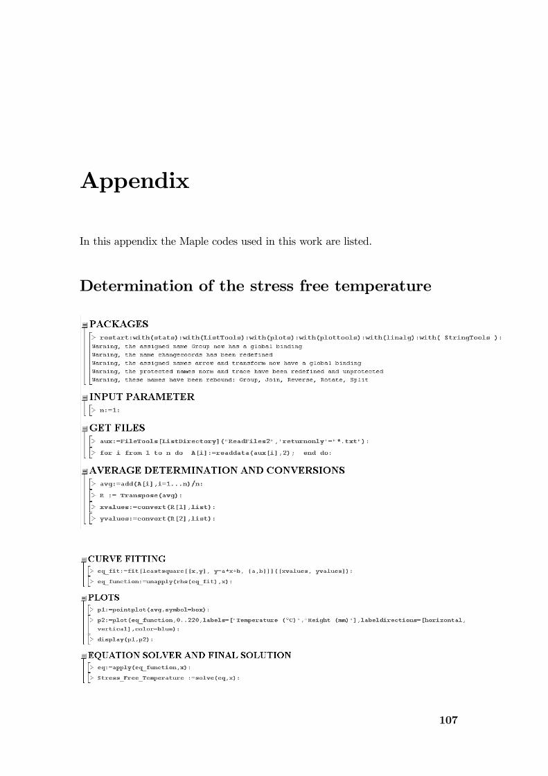
Appendix
In this appendix the Maple codes used in this work are listed.
Determination of the stress free temperature
107
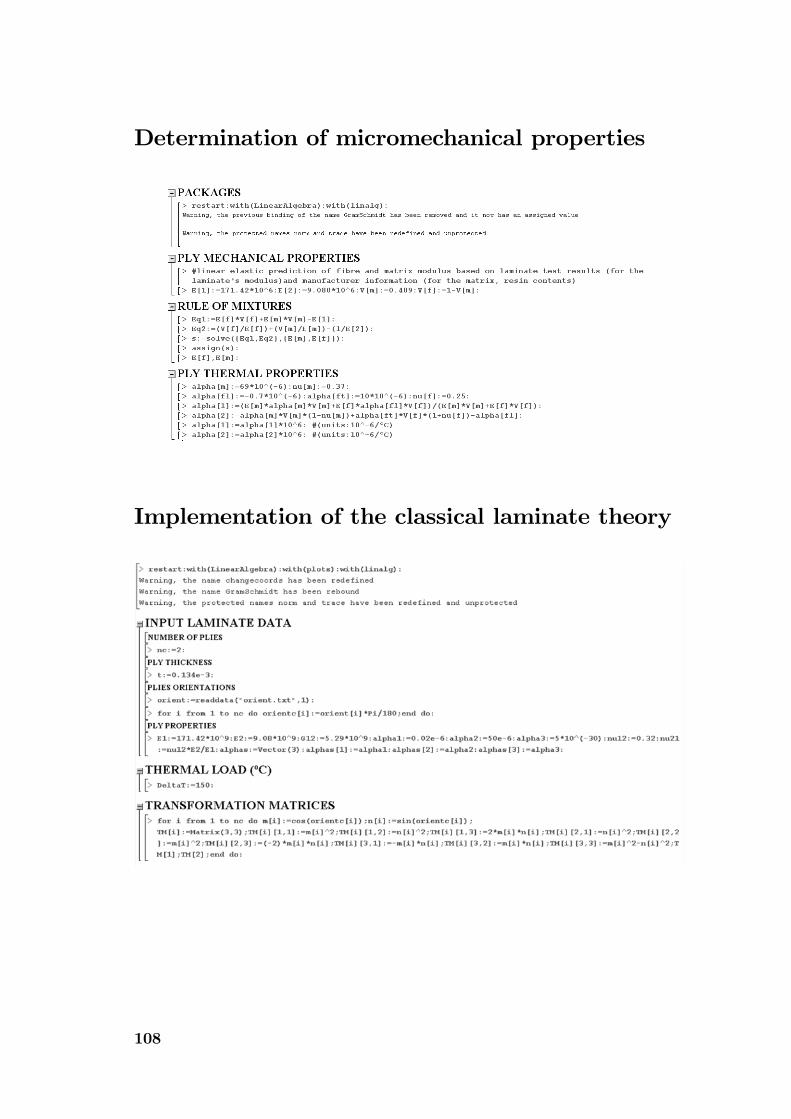
Determination of micromechanical properties
Implementation of the classical laminate theory
108

109
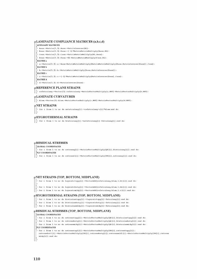
110


![L5 High Five Lachman.pptx [Read-Only] - IHI Home Pageapp.ihi.org/.../Document-11517/Presentation_L5_High_Five_Lachman.pdf · 11/29/2016 2 Key content of The High Five Improving Access](https://img.pdfslide.net/doc/110x75/5e19beb513040b6db9117d64/l5-high-five-read-only-ihi-home-pageappihiorgdocument-11517presentationl5highfivelachmanpdf.jpg)