Embed Size (px)
Citation preview

RACING CAR DETECTION USING CASCADED
CLASSIFIER
HO SECK WEI
FACULTY OF ENGINEERING
UNIVERSITY OF MALAYA
KUALA LUMPUR
2017

RACING CAR DETECTION USING CASCADED
CLASSIFIER
HO SECK WEI
THESIS SUBMITTED IN PARTIAL FULFILMENT OF
THE REQUIREMENTS FOR THE MASTER’S DEGREE
OF MECHATRONICS ENGINEERING
FACULTY OF ENGINEERING
UNIVERSITY OF MALAYA
KUALA LUMPUR
2017

iii
UNIVERSITY OF MALAYA
ORIGINAL LITERARY WORK DECLARATION
Name of Candidate: HO SECK WEI (I.C/Passport No:
Matric No: KQF 160001
Name of Degree: Master Degree of Mechatronics Engineering
Title of Thesis : Racing Car Detection Using Cascaded Classifier
Field of Study: Imaging Processing
I do solemnly and sincerely declare that:
(1) I am the sole author/writer of this Work;
(2) This Work is original;
(3) Any use of any work in which copyright exists was done by way of fair dealing
and for permitted purposes and any excerpt or extract from, or reference to or
reproduction of any copyright work has been disclosed expressly and
sufficiently and the title of the Work and its authorship have been
acknowledged in this Work;
(4) I do not have any actual knowledge nor do I ought reasonably to know that the
making of this work constitutes an infringement of any copyright work;
(5) I hereby assign all and every rights in the copyright to this Work to the
University of Malaya (“UM”), who henceforth shall be owner of the copyright
in this Work and that any reproduction or use in any form or by any means
whatsoever is prohibited without the written consent of UM having been first
had and obtained;
(6) I am fully aware that if in the course of making this Work I have infringed any
copyright whether intentionally or otherwise, I may be subject to legal action
or any other action as may be determined by UM.
Candidate’s Signature Date:
Subscribed and solemnly declared before,
Witness’s Signature Date:
Name:
Designation:

iv
ABSTRACT
Human error tends to occur especially when it comes to recognizing or detecting an
object, the situation becomes worst when human has made the wrong judgement due to
poor observation skills, causing a side effect to what happens subsequently. To minimize
these wrong judgement, machine learning is proposed to assist them via detection and
classification. Machine vision system is one of the technology where it will be a great
useful application in the near future for it will enable a system to analyze and
communicate with other devices to run its respective task. The general concept of how a
machine vision system works is fully based on the fundamental of image processing,
therefore the main requirement for a machine vision system is combination of both
hardware and software to execute its task. This study is performed to detect racing cars
from any sources that are obtained with a robust, stable and high efficiency.
v
ABSTRAK
Kesalahan manusia cenderung berlaku terutamanya apabila mengenal pasti atau
mengesan objek, keadaan menjadi semakin memburuk apabila mereka membuat sesuatu
keputusan yang salah disebabkan pemerhatian yang buruk, hal ini menyebabkan kesan
sampingan kepada apa yang berlaku seterusnya. Untuk mengurangkan penghakiman yang
salah ini, pembelajaran mesin dicadangkan untuk membantu mereka melalui pengesanan
dan klasifikasi. Sistem Pengilhatan Mesin adalah salah satu teknologi yang merupakan
aplikasi yang berguna dalam masa yang akan dating disebabkan keupayaan untuk
membolehkan sistem ini menjalankan analisasi dan komunikasi dengan peralatan lain
untuk menjalankan tugas masing-masing. Konsep umum bagi sistem penglihatan mesin
berfungsi sepenuhnya berdasarkan asas konsep pemprosesan imej, oleh itu keperluan
utama untuk sistem penglihatan mesin adalah gabungan antara perkakasan dan perisian
untuk melaksanakan tugasnya. Kajian ini mencadangkan untuk mengesan kereta lumba
dari mana-mana sumber yang terdapat dalam kaedah yang bercekap, stabil dan
mempunyai kecekapan yang tinggi untuk membantu manusia menyelesaikan masalah ini.
.

vi
ACKNOWLEDGEMENTS
First of all, I would like to express gratitude to my advisor, Ir. Dr. Chuah Joon Huang.
I have been amazingly fortunate to have a supervisor who has given me the freedom to
explore things on my own, and with his patient guidance whenever my steps are faltered.
His kindness and support have helped me to overcome many critical situations throughout
my project. It has been a great pleasure to work under him as one of his research project
students.
A special thanks to my family members for sharing their understandings and helping
me in terms of my finance in my study. Their passionate belief in the education has
encourage me to excel academically. Their strong values have formed who I am today
and will continue to do so.
Lastly, I would like to thank to those who has helped me in research project directly
or indirectly.

vii
TABLE OF CONTENTS
Abstract ............................................................................................................................ iv
Abstrak .............................................................................................................................. v
Acknowledgements .......................................................................................................... vi
Table of Contents ............................................................................................................ vii
List of Figures .................................................................................................................. ix
List of Tables.................................................................................................................... xi
List of Symbols and Abbreviations ................................................................................. xii
List of Appendices ......................................................................................................... xiii
CHAPTER 1: INTRODUCTION .................................................................................. 1
1.1 Background .............................................................................................................. 1
1.2 Problem Statement ................................................................................................... 2
1.3 Objectives ................................................................................................................ 3
1.4 Scope........................................................................................................................ 3
1.5 Thesis Organization ................................................................................................. 3
CHAPTER 2: LITERATURE REVIEW ...................................................................... 5
2.1 Introduction.............................................................................................................. 5
2.2 Viola-Jones Algorithms ........................................................................................... 6
2.3 Object Detection ...................................................................................................... 8
2.3.1 Coarse-to-Fine and Boosted Classifier ..................................................... 11
2.3.2 Dictionary Based ...................................................................................... 12
2.3.3 Deformable Part-Based Model ................................................................. 13
2.3.4 Deep Learning .......................................................................................... 14
2.3.5 Trainable Image Processing Architectures ............................................... 17

viii
2.4 Feature Extraction .................................................................................................. 18
CHAPTER 3: METHODOLOGY ............................................................................... 23
3.1 Introduction............................................................................................................ 23
3.2 Flowchart ............................................................................................................... 24
3.3 Modelling and Programming ................................................................................. 26
3.4 Conclusion ............................................................................................................. 32
CHAPTER 4: RESULTS AND DISCUSSIONS ........................................................ 34
4.1 Introduction............................................................................................................ 34
4.2 Theoretical Experiment for Object Detection........................................................ 34
4.3 Results.................................................................................................................... 35
4.4 Discussion .............................................................................................................. 41
4.5 Error of Analysis.................................................................................................... 42
4.6 Summary ................................................................................................................ 43
CHAPTER 5: CONCLUSION ..................................................................................... 44
5.1 Introduction............................................................................................................ 44
5.2 Conclusion ............................................................................................................. 44
5.3 Recommendation for Future Project ...................................................................... 45
References ....................................................................................................................... 46
Appendix A ..................................................................................................................... 49

ix
LIST OF FIGURES
Figure 2.1: Two rectangular features shown in (A) and (B). (C) shows three rectangular
features and (D) shows four rectangular features [1]. ....................................................... 7
Figure 2.2: Facial Recognition that is based on Viola-Jones algorithm [1]. ..................... 8
Figure 2.3: Pedestrian detection using Multi-Stage Particle Windows [13]. .................. 10
Figure 2.4: Shoe Detection using Key Points Finding [14]. ........................................... 10
Figure 2.5: Block Diagram of the Unified Learning Framework for Face Detection [15].
......................................................................................................................................... 12
Figure 2.6: Classification of Bicycle using Dictionary Based Detection [16]. ............... 13
Figure 2.7: A Venn Diagram That Shows Deep Learning Is a Subset of Artificial
Intelligence, Machine Learning and Representation Learning [20]................................ 15
Figure 2.8: Schematic Levels of Each Learning [20]. .................................................... 15
Figure 2.9: Proposed Deep Model for Pedestrian Detection [22]. .................................. 16
Figure 2.10: Architecture of Framework for Trainable Image Processing for Humanoid
Robot by Leitner et al. [23]. ............................................................................................ 17
Figure 2.11: Sample Blurred Image [26]. ....................................................................... 20
Figure 2.12: Harris Corner Detection Result [26]. .......................................................... 21
Figure 2.13: SURF Detector Result [26]......................................................................... 21
Figure 2.14: SIFT Detector Result [26]. ......................................................................... 22
Figure 3.1: Flowchart of Analysis. .................................................................................. 25
Figure 3.2: Python Command Windows. ........................................................................ 27
Figure 3.3: Each Teams Are Separated into Different Folders. ...................................... 27
Figure 3.4: Negative Images. .......................................................................................... 28
Figure 3.5: Positive Image (Sauber Racing Team) infused into the Negative Image. .... 29
Figure 3.6: Text File That Describe the Coordinate of Each Positive Image in the Negative
Image. .............................................................................................................................. 29

x
Figure 3.7: A Completed Training Stage. ....................................................................... 30
Figure 3.8: Content in the XML File. ............................................................................. 31
Figure 3.9: Programming Code in Python with XML File Defined into the Detection
System. ............................................................................................................................ 32
Figure 3.10: Steps of the Training Stages. ...................................................................... 32
Figure 4.1: Detection of Ferrari Racing Team. ............................................................... 35
Figure 4.2: Detection of Force India Racing Team......................................................... 35
Figure 4.3: Detection of Haas Racing Team. .................................................................. 36
Figure 4.4: Detection of Manor Racing Team. ............................................................... 36
Figure 4.5: Detection of McLaren Racing Team. ........................................................... 37
Figure 4.6: Detection of Mercedes Racing Team. .......................................................... 37
Figure 4.7: Detection of Red Bull Racing Team............................................................. 37
Figure 4.8: Detection of Renault Racing Team. ............................................................. 38
Figure 4.9: Detection of Sauber Racing Team. ............................................................ 38
Figure 4.10: Detection of Toro Rosso Racing Team. ..................................................... 39
Figure 4.11: Detection of Williams Racing Team. ......................................................... 39
Figure 4.12: Original Image for Detection. ..................................................................... 40
Figure 4.13: Detection of Ferrari Racing Team and Williams Racing Team. ................ 40
Figure 4.14: Video Detection for Ferrari Racing Team. ................................................. 41

xi
LIST OF TABLES
Table 3.1: Training Result for Each Team. ..................................................................... 31
Table 4.1: Error of Analysis on Racing Car Detection. .................................................. 42

xii
LIST OF SYMBOLS AND ABBREVIATIONS
ANN : Artificial Neural Networks
BoW : Bag-of-Words
CNN : Convolutional Neural Network
DoG : Difference of Gaussians
GPUs : Graphical Processing Units
GUI : Graphical User Interface
ROI : Regions of Interest
SIFT : Scale-Invariant Feature Transform
SURF : Speeded-Up Robust Features
V-J : Viola-Jones
XML : Extensible Markup Language

xiii
LIST OF APPENDICES
Appendix A............................................................................................................. 43

1
CHAPTER 1: INTRODUCTION
1.1 Background
Machine vision system is one of the technology where it will be a great useful
application in the near future for it will enable a system to analyze and communicate with
other devices to run its respective task. The general concept of how a machine vision
system works are fully based on the fundamental of image processing, hence the
requirement for a machine vision system is combination of both hardware and software
to execute its task.
In the industries, these systems are required for a greater robustness, stability and
efficiency, these requirements are important as it will yield in different types of
productions, improve the manufacturing process and ensure the safety of the workers in
their working field. However, some of the application are still required to perform
manually with the machine due to lack of researching and instability of the systems to
perform automatically, causing extra workforce in order to hire a person to operate the
machine manually.
Image processing is a step that will convert the image data into a digital form, by using
this information, it will enable the particular system to analyze it and perform the specific
task more easily, however these algorithms requires a few stages in order to make the
system to be able to apply it on the field, one of the most important stages for this system
is to learn from the conceptual object first in order to be able to be detected in the field
[1]. However, it has some disadvantages especially when the properties of recognition are
same as the other object, for examples size or color. Suitable algorithm and methods are
required to ensure that a higher probability/success rate will be achieve to be able to detect
the correct object.

2
Object detection has been a widely used application in this decade, a frequently used
application for detection is facial recognitions which these applications can be seen in
camera’s function, however object detection is not frequently used in both industry as
well as the commercial due to the complexity of the algorithms. Taking an example in the
sports sector, some judges or commentators are still not relying on object detection system
for their working purpose, this can cause human errors which wrong judgement was
called upon during that instance.
To assist both judges and commentators or any users, a study of object detection has
been conducted. To simplify the study purpose, racing cars has been selected for this
studies that will be related to the proposed Research Project title, “Racing Car Detection
Using Cascaded Classifier”.
1.2 Problem Statement
The aim of this project is to determine the best method for object detection because
different objects have different characteristics. Theoretically, a successful detection is
solely based on features, data sizes, quality of the images etc. The situation arises when
some of the testing data will be detected wrongly due to the same properties as the
wrongly classified learning data. For example, the system might misclassify a team of
racing car as another team due to the existence of wheel on both racing cars. Besides that,
an unsupervised algorithm is needed in order to ensure that the system will be user
friendly by the user without continuously supervising it to ensure the task are done
correctly. With this object detection, the users will be able to track any different teams of
racing cars that they wish for analyze purposes, this could reduce any potential human
errors that will incurred in the near future.

3
1.3 Objectives
The objectives of this research are stated as below:
1. To study the detection method on any objects for performing subsequent object
recognition.
2. To understand how feature extraction method will used on an object for object
recognition.
3. To design an object recognition system that will improve the efficiency of the
system.
1.4 Scope
This study will cover on how cascaded training will be used for object detection
applications since it is commonly used for pattern recognition applications. Besides that,
as stated earlier, different team of racing cars has different features that represents each
of them respectively, therefore an unsupervised learning is used to determine the accuracy
of the system since cascaded training can be supervised learning or unsupervised learning.
At the end of the study, different teams of racing cars will be able to be detected correctly
with minimum error.
1.5 Thesis Organization
This thesis is organized in five chapters. In Chapter 1, the explanation for the project
which will be given in a general term, problem statements of this project will be
elaborated followed by the scopes of the project will be covered in this project.
Chapter 2 describes the fundamental the fundamental of object detections and any
relative trainings that can be used for object detection. It will further discuss about the
characteristic and applications used in cascaded learnings or any other terms that can be
related to the project.

4
In Chapter 3, it describes the methodology on how to develop the systems that can
detect the racing cars correctly for this project.
As for Chapter 4, the results that are obtained are discussed as well as both discussions
and analysis for this project. The strength and weakness of this project are also discussed
in this chapter.
Finally, in Chapter 5, a conclusion is made for this project and recommendations for
future works for this project will be the ending for this thesis.

5
CHAPTER 2: LITERATURE REVIEW
2.1 Introduction
This chapter discusses about the theoretical background on understanding of detection
applications in image processing. It is important to understand how image processing is
used for detection purposes by understanding its fundamental algorithms. The common
algorithms that was used for detection in image processing is the facial detection, which
is the Viola-Jones algorithm, designed by both Paul Viola and Michael Jones in the year
of 2001 [1]. Further studies were made by researchers around the globe that further
enhance this algorithm, Nguyen and et al. has created a software based on the Graphical
Processing Units (GPUs) by implying Viola-Jones algorithms in it. Xu. et al. have
conducted a study that further enhanced the V-J algorithms that was used for vehicle
detection on unmanned aerial vehicle imagery.
The algorithm of object detection was further enhanced by combinations of V-J
algorithms with other algorithms such as Artificial Neural Networks (ANN) [4],
AdaBoost algorithms and et cetera. Rashidan et al. has studied on conducting the analysis
of Artificial Neural Network and V-J Algorithm based on moving object detection [4].
Peleshko and Soroko has made a research on the usage of Haar-like features and
AdaBoost algorithm in V-J method for object detection [5].
Further enhancement was made when researchers started conducting their studies onto
video-based detection by various algorithms. Wu et al. has conducted a study by using 5
layers of CNN as their classifier for real-time running detection from a moving camera
[6]. Guo has studied an efficient method for object tracking algorithms of a video by using
a dynamic model that is optimized in mean-shifted algorithms [7].

6
2.2 Viola-Jones Algorithms
A common application of detection in image processing is face detection in the early
2000s which was created by Paul Viola and Michael Jones [1] on an algorithm that has
the ability of quick object detection using a boosted cascade of features which comprises
of three key contributions: Integral Images, Learning Algorithms and Cascading.
Integral Images are the images that allows the features for detection to be computed
quickly which these images represent the images with similar summed up area of table
used in the computer graphics done by Crow [9], these images can be computed by using
a few operations per pixels. Once the images are computed, Haar-like features will be
able to compute at any scale or location at a certain of time.
Learning Algorithms is a simple and efficient classifier that is built by Freund and
Schapire [8], this algorithm is also known as AdaBoost algorithm that was built based on
selecting a small number of features which are important from the library of features. This
algorithm uses the Haar-like features which is larger than number of pixels in each image
sub-window that will ensure that the learning process will be executed faster than pixels
and will exclude the majority of features but focused on the critical features only. Tieu
and Viola have conducted a study by using AdaBoost algorithm to constraint the weaker
classifier by depending only a single feature, as a result they are able to obtain a boosting
process on each stages of classification, with each times of feature selections, a new
weaker classifier is produced [10]. This has improved the efficiency of the classifications
on every stage as the stages goes on.
Cascading is a method that combines the classifiers to discard the background regions
quickly and computing on object-like regions. This method will combine the successful
complex classifier in a cascade structure that will improve the speed of detection that
focus mainly on the promising regions on each image. With cascading is being implied

7
into the algorithm, the algorithm will focus more attention into the promising region,
which unrelated images will be filtered out to ensure a shorter time is used for detection.
Cascading are proposed by both Viola and Jones to be constructed during the early stages
in order to reject a majority of images and focus subsequently for promising regions at
the late stages [1].
Besides that, Viola and Jones had also used the Haar basis function which harbors
based on using the features rather than pixels, resulting easier to process and higher
efficiency for detection. Figure 2.1 shows the rectangular features shown relative to the
enclosing detection windows where the sum of the pixel in white region is subtracted
from the black region within the rectangular.
Figure 2.1: Two rectangular features shown in (A) and (B). (C) shows three
rectangular features and (D) shows four rectangular features [1].
Based on all the contributions that have been mentioned earlier and the Haar basis
function, Viola and Jones were able to construct the V-J algorithms that was used for
facial recognition. Figure 2.2 shows results of the facial detection that was based on the
V-J algorithms.

8
Figure 2.2: Facial Recognition that is based on Viola-Jones algorithm [1].
2.3 Object Detection
Object detection is an expansion of computer vision research which adapted from the
machine learning methods. Detection was made by determining the location and the scale
of the object at particular instances based on a set of classes of objects. Further
information was extracted from the detected objects during the detection progress.
Depending on the applications, some of the detection were made based on multiple object
classes while others were made with single object class [11].
Vershae and Ruiz have gathered surveys on detections and recognitions that has been
published worldwide and have concluded four main problems that are related to object
detections, these problems are object localization, object presence classification, object
recognition and view and pose estimation [11].
Object detection is described as the determination of the location and the scale of the
single object based on the particular image. Object presence classification is corresponded
with determining the object towards a suitable class based on the image without any
information given. Object recognition is defined as determining the object specified

9
correctly based on the image and finally, view and pose estimation is the view and
position of the object are determined based on the image [11].
In the early days, Fischler and Elschlager have proposed using template based
matching technique for object detection before V-J algorithm was introduced [11 – 12].
As the times goes on, more algorithm has been introduced after V-J algorithms such as
Neural Networks, Support Vector Machining and et cetera. When studies of facial
detection have reached the peak point, studies on computer vision detection has start to
diverting towards objects that people are often to interact with, such as pedestrians, body
parts and et cetera. Most of these object detections are based on the same basic scheme,
which is known as the sliding window, the function of sliding window is to detect the
object appearing in the image in different location and scales with an exhaustive searching
using a classifier [11]. The classifier usually works on a given scale or size of the sample
data and classify the test data that have different versions and sizes. Besides sliding
window technique, there are some other alternatives as well. Bag-of-Words (BoW) is one
of the alternatives which used to verify the presence of the objects on the image [13]
where in some cases it might have a better efficiency than other algorithms. Multistage
particle windows or samples patches is another alternative that can be used which aimed
to reduce exhaustive search all over the images, Prati et al. has conducted research by
using multistage particle window for pedestrian detection, Figure 2.3 shows how
multistage particle works where the distribution of particles are spread across the
windows of image in every stages, when the number of stages increased, the particles has
started to accumulated onto some area, these area are known as Regions of Interest (ROI).

10
Figure 2.3: Pedestrian detection using Multi-Stage Particle Windows [13].
Another alternative used is key points findings, unlike the previous two alternatives
that are mentioned which performs classifications based on reducing the number of image
patches, key points finding is done by finding the features that representing the particular
object and matches them with the test images, where Azzorpardi and Petkov have made
a study to understand the limitation of key points finding by detecting the shoes in
different complex scenes. Figure 2.4 shows the detection that was made by Azzorpardi
and Petkov [14].
Figure 2.4: Shoe Detection using Key Points Finding [14].
Although there are a few alternatives that can be used for object detections besides
algorithms such as V-J algorithms and et cetera, however according to Vershae and Ruiz

11
thinks that these alternatives does not guarantee that all the objects will be detected during
the particular instances [11]. Therefore, object detection has moved into a more advanced
approach which is split into few categories, where each categories has their own pros and
cons.
2.3.1 Coarse-to-Fine and Boosted Classifier
This category is considered the most popular approaches, one of the commonly used
boosted cascaded classifier that was introduced is the V-J algorithms that has been
mentioned earlier [1]. The classifier has a better efficiency in rejecting the test data
through the filters, but unlike the multi-stage particles, the boosted classifier does not
correspond with the image patches onto the object in the image. This classifier is
commonly used due to generating an additive classifier which is easy to control the
complexity of each stages during the classification and boosting can be used for feature
extraction during training. When efficiency is the key requirement, the coarse-to-fine
classifier is proposed as the suitable object detection classifier, one of the example is face
detection that was studied by Verschae and Ruiz using a unified learning framework for
detection and classification using a nested cascade of boosted classifier [15]. Figure below
shows the block diagram of the unified learning framework that was done by Verschae
and Ruiz [15].

12
Figure 2.5: Block Diagram of the Unified Learning Framework for Face
Detection [15].
2.3.2 Dictionary Based
Dictionary Based is an approach where a dictionary of features will be shared across
all the categories, allowing all images to be in the same feature of space for classification
purpose [16]. A study was done by Mutch and Lowe using this concept for class
recognition with limited receptive fields, this approach was used because it was designed
for single object detection per image only. Therefore, this approach is not robust for
handling if two or more objects appeared in the image as well as the localization of the
object is might not be accurate compare to another category. Figure below shows one of
the result obtained from Mutch and Lowe during their studies.

13
Figure 2.6: Classification of Bicycle using Dictionary Based Detection [16].
From Figure 2.6, we have observed that there is some misclassification from the result
obtained by Mutch and Lowe. Therefore this has justify that this approach cannot be
handled robustly well and there are some accuracy issue.
2.3.3 Deformable Part-Based Model
This category is considered to be robust compare to other approaches which consider
both object and part models in the image as well as their relative positions. However,
Verschae and Ruiz also noted that this approach is rather time-consuming comparing to
other approaches during training and this approach has a difficulty in detecting an object
which are small in scales. A relevant study was made by Yan et al. by developing a faster
deformable part-based model for object detection by modifying the model into a cascaded
Deformable Part-Based Model for a faster evaluation since speed is a bottleneck for this
model, the method that was proposed by Yan et al. were observed to have an increase of
four times the speed faster than traditional model [17].

14
2.3.4 Deep Learning
Deep learning is a subset of artificial intelligence, which is commonly known as the
machine learning. Deep learning will evaluate the examples from the model that was
given by the user and execute based on the instructions that has been given instead of
being taught by a massive list of rules for problem solving [18]. If a well-suited model is
designed, this model will be able to solve a complex problem with good accuracy.
According to Deng and Yu [19], deep learning is a type of algorithm that uses a
cascaded non-linear model that uses for feature extraction and transformation. The model
can be a supervised or unsupervised algorithm that can be used in pattern or statistical
classification. The algorithm is learning a multiple level of representation that will
correspond with different levels of abstractions which are in the form of hierarchy
concepts.
According to Goodfellow et al. [20], Deep learning is the only reliable approach on
building an Artificial Intelligence system that can operate in the real-world environment
as a machine learning. Deep learning has a better flexibility by learning any representation
in the world since it is a kind of representation learning with has a higher level of
schematics of process, this can be shown is Figure 2.7 and Figure 2.8 respectively.

15
Figure 2.7: A Venn Diagram That Shows Deep Learning Is a Subset of Artificial
Intelligence, Machine Learning and Representation Learning [20].
Figure 2.8: Schematic Levels of Each Learning [20].

16
Bengio et al. have concluded that in although many deep learning algorithm were
framed as an unsupervised learning instead of supervised learning which will label the
information that are readily available for training and more focusing on feature
engineering, these unsupervised algorithm will make full use of the unlabeled data that
were given where supervised algorithm cannot do that, making the unsupervised learning
has a better benefit than supervised learning because these unlabeled data are usually
more abundant comparing to the labelled data.
Vershae and Ruiz [11] have stated that the key difference between deep learning and
other approaches that have been mentioned previously is this approach is learned from
the feature representation rather than being designed by the user, however this will bring
forth a drawback which is a large amount of sample data are required for deep learning
to undergo training in order to ensure a good accuracy can be achieved. A study of
detecting pedestrian using Deep Learning was done by Ouyang and Wang [22], since
pedestrian are considered to have a non-rigid deformation in the image, Ouyang and
Wang has designed a deep model by convolving the image with a smaller size filter into
a numbers of feature maps so that these feature maps can be processed by continuous
layer before reasoning model are able to estimate the detection.
Figure 2.9: Proposed Deep Model for Pedestrian Detection [22].
17
Based on the designed deep model, Ouyang and Wang are able to obtained an
improvement of detection by reducing the average miss detection rate than usual.
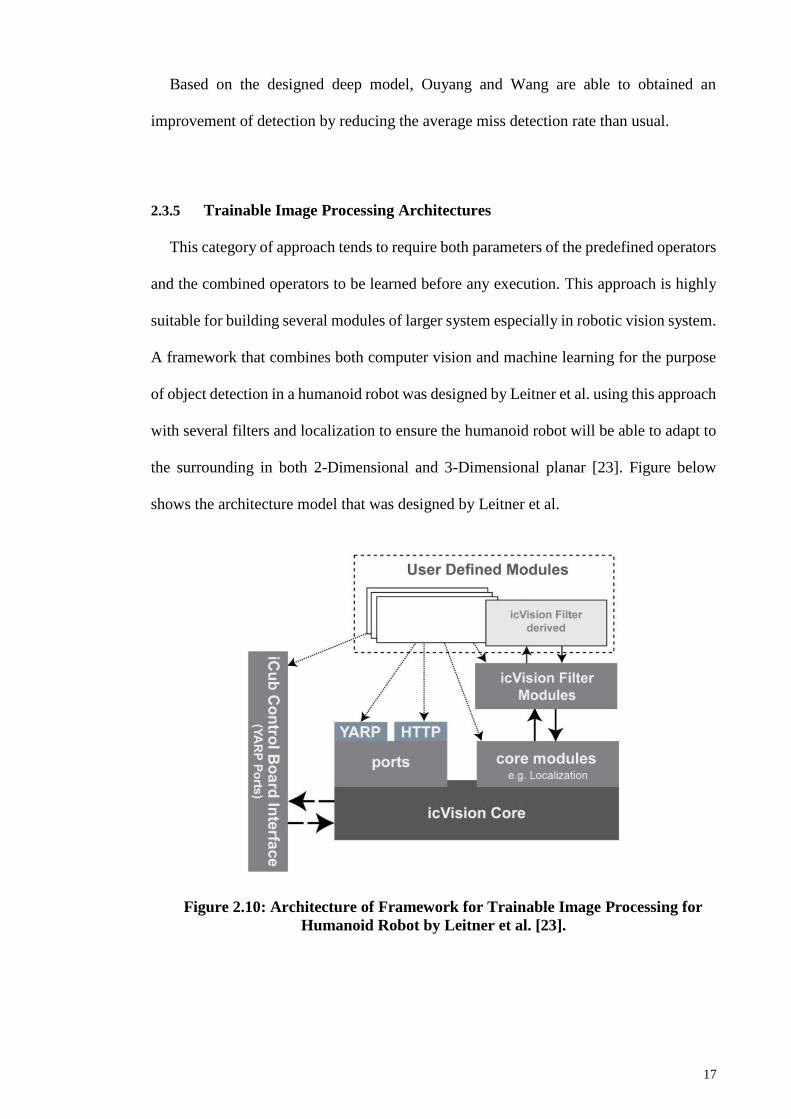
2.3.5 Trainable Image Processing Architectures
This category of approach tends to require both parameters of the predefined operators
and the combined operators to be learned before any execution. This approach is highly
suitable for building several modules of larger system especially in robotic vision system.
A framework that combines both computer vision and machine learning for the purpose
of object detection in a humanoid robot was designed by Leitner et al. using this approach
with several filters and localization to ensure the humanoid robot will be able to adapt to
the surrounding in both 2-Dimensional and 3-Dimensional planar [23]. Figure below
shows the architecture model that was designed by Leitner et al.
Figure 2.10: Architecture of Framework for Trainable Image Processing for
Humanoid Robot by Leitner et al. [23].

18
2.4 Feature Extraction
For moving objects in a non-stationary background, classification using feature
extraction has become an important part of detection that created a vast area for study.
With an instance of detection to be obtained, the feature extraction algorithms have
become a well-recognized algorithm for applying into the real-world detection
applications. This algorithm is suitable to be used with equipment such as digital camera,
traffic camera and etc. Feature extraction is done within the test image by recognizing the
object based on the information from the reference image. This algorithm will act as the
signature to the image that detects meaningful features, which is known as the feature
descriptors from the database given [25].
According to Lal and Arif, there are a wide variety of algorithm that represents feature
extraction such as Harris Corner Detector, Scale-Invariant Feature Transform (SIFT),
Speeded-Up Robust Features (SURF), K-Mean Clustering and etc where Harris, SURF
and SIFT are adopted from key point features detection [26].
Harris Corner is a detection algorithm that detects the corner by forming a local search
windows that will be shifting the window pixel-by-pixel in all direction. The variance of
the pixel intensity will help the algorithm to detect both high and low brightness level
where the shifting process will mean the variation of the pixel intensity. Along the
shifting, when a significant changes of pixel intensity is detected, the corner will be
detected, however, when there are no pixel intensity changes along the edge, an edge
region is detected [26].
Scale-Invariant Feature Transform (SIFT) detector consist of four main stages which
are the space extrema detection, key point localization, orientation computation and key
point descriptor extraction. Scale-space extrema detection identify the potential key
points when severeal Gaussian blurred images at different scales are produced by the

19
input image using the Difference of Gaussians (DoG). The DoG will then compute from
neighbours in scale space before proceeding to next stage, which is the key point
localization which the candidate key points found in DoG will be determined whether the
value will against the ratio of eigenvalues of the Hessian matrix, those unstable key points
will be eliminated at this stage. At third stage, the computation will assign a principal of
orientation to each key point before entering the final stage, which will compute a highly
distinctive descriptor for each key point which results each feature will become a vector
for the descriptors to analyze [27].
The SURF Detector on the other hand employs the integral image and efficient scale
space construction in order to generate efficient key points and descriptors. Unlike SIFT,
SURF only require two stages, key point detection and key point description. During the
first stage, the integral image undergoes fast computation of approximation using
Laplacian of Gaussian images via box filter. Once obtaining the Hessian matrix, the
determinants is then used to detect the key point, hence the SURF will be build to its own
scale space by keeping the image size same while varying the filter size. On the second
stage, which is the final stage, each detected key points will be assigned for a reproducible
orientation which is in linear axis, the descriptor will then be computed by constructing a
window square centering around the key points and oriented along the orientations that
have been obtained before. The SURF descriptor will be invariant in terms of rotation,
scale and contrast while partially invariant to other transformations [28].
The K-Mean Clustering is a typical clustering algorithm that undergo the process of
searching for data points which are close within the point at a specific range. It involves
of grouping the data into a disjoined cluster so that the number of each cluster would be
approximately the same among all clusters throughout the image. K-mean is a simple
algorithm that has fast computational time by partitioning each cluster into k cluster that
are represented by an adaptive-changing centroid, these centroid are known as the cluster

20
center. Like all data analysis, the k-mean will start from some random initial values which
is known as the seed-points, then it will compute the square distances between the inputs
and the centroids before assigning the input to the nearest centroid. As the algorithm
further cluster into k disjoint subsets, the will minimize the mean square error function
[29].
Lal and Arif has conducted study of feature extractions on blurred image using a few
of the algorithms that has been mentioned. Figure 2.11 shows the sample blurred image
that will be used for their study.
Figure 2.11: Sample Blurred Image [26].
The cyclist in the blurred image will be acting as a moving object for the study. Using
the Harris Corner Detection, the image turns out to be sharp with lesser noise and a
significant of points are detected, there are no points that are detecting the background.
Figure 2.12 shows the result of Harris Corner Detection.

21
Figure 2.12: Harris Corner Detection Result [26].
The sample image was then being tested using SURF algorithm and SIFT algorithm,
Lal and Arif concluded that these feature detectors will still work well on blurry images
by detecting sufficient points on the moving object. They also concluded that SURF
algorithm was able to detect more points in the background comparing Harris and SIFT.
Figure 2.13 shows the result using SURF algorithm while Figure 2.14 shows the result
using SIFT algorithm.
Figure 2.13: SURF Detector Result [26].

22
Figure 2.14: SIFT Detector Result [26].
From this study, Lal and Arif made a conclusion that although both Harris Corner
Detection and SURF Detector are able to process the information relatively faster than
SIFT Detector, but Harris Corner Detection are seemingly more susceptible to noise and
smooth pixel intensity level while SIFT Detector will detect the maximum amount of
feature points, causing a longer processing time. SURF Detector on the other hand are
able to detect a considerable amount of points towards moving object as well as
backgrounds, which will make the computation involve in differentiating between
background and foreground much easier than Harris Corner Detection [26].

23
CHAPTER 3: METHODOLOGY
3.1 Introduction
Based on the Literature Reviews that has been discussed on Chapter 2 previously, this
chapter discusses about the suitable method that can be applied onto the study. Based on
Chapter 2, it is found that a cascaded training is suitable for this study since cascaded
training will be able to assist the system to detect the object that was required with the
capability of machine learning. Besides that, a cascaded classifier is proposed to be used
in this study so that a shorter time with high efficiency of detection can be achieved by
the system. The focus is to design a guarantee detection of racing car, which in this study,
the scenario for racing cars will be Formula One racings for study purposes.
A programming will be explained at the end of this chapter to explain the flow process
of the system with a simplified flow chart. The applications that was used in this study
will be briefly explained as well. At the end of this chapter, the system will be able to
conduct detection of racing cars on each team in Formula One racings in both imagery
and video.

24
3.2 Flowchart
Start
Conduct literature
Obtain a set of positive
images and negative image
Define the fixed sizes
of both positive image
and negative image
measurement
Grayscale both positive
image and negative image
Random rotate the
positive image into the
negative image
All data
trained?
Create vector file for
the positive image.
No
Cascade training for the
positive image.
Yes

25
Figure 3.1: Flowchart of Analysis.
Based on the Figure 3.1, the explanation of the design and analysis of the racing car
detection using a cascaded classifier will be done. A literature review and feasible studies
were made in order to select the proper method to conduct the study since there are many
methods for object detection as explained in Chapter 2. At the end of the process, a
System undergo
detection from other test
sources.
Labelling and framing the
detected object.
Conclude research
Detection
complete?
Yes
Analyze the result
No
New
Detection?
No
Yes
Project complete

26
conclusion of the technique that was used in the project will be made and further
recommendations for future works are proposed.
3.3 Modelling and Programming
To ensure an accurate object detection can be achieved a large number of images have
to be collected for both positive images and negative images. Positive images are referred
as the images that represents the object that will be detected from the test samples while
negative images are images that does not have any relationships with the object that will
be detected.
Both positive images and negatives images are taken from any sources available, to
ensure that an optimum machine learning can be done, all the images are resized
accordingly. The negative images are downloaded and converted into grayscale with a
size of 1000x1000 pixels while the positive images are resized to 800x600 pixels using
Python, a multi-programming language platform that most of the data processing modules
are based on C language or C++ language with a much simpler Graphical User Interface
(GUI) [24]. Python is widely used in many applications because of the capability to adapt
to real time user requirements such as security, simulations, precision calculation etc.
Figure 3.2 shows the Python command windows that will be involved in the study.

27
Figure 3.2: Python Command Windows.
In this study, a total of 11 teams in the Formula One racings are the positive images
for detection. These images are taken from the web and predefined as the sample data,
each teams’ images are stored in separated folders so that the system can detect each team
accordingly while the negative images are downloaded into a separated folder.
Figure 3.3: Each Teams Are Separated into Different Folders.

28
Figure 3.4: Negative Images.
A total of 2,292 negative images are collected for this study. Once this procedure is
done, each of the positive images will then be infused onto these negative images with
random rotation of the positive image in the negative images, this is to ensure that the
number of positive images should be at least one times larger amount than the negative
image so that the system will be able to classify the object more accurately. When this is
being done, a text file will be created with a coordinate written on it to mark the coordinate
of frame for indicating the position of the positive image. This is to separate out the
positive image out from the negative image.

29
Figure 3.5: Positive Image (Sauber Racing Team) infused into the Negative
Image.
Figure 3.6: Text File That Describe the Coordinate of Each Positive Image in
the Negative Image.
This text file is then being brought forward for further processed with further resizing
of 20x20 pixels as an input training for the system classifier, this file is known as the
vector file. Vector file also describes the background of each images in a more thorough
way for training purposes. Once the vector file is created, the vector file will be set as the
input for the classifier training, an Extensible Markup Language (XML) file is created at

30
the end of the training, this file is used as the library sources for the detection system.
During the training, the training samples will undergo few stages of training depending
on the quality of the images. At each stage, the input will be taken from the output of the
previous stage for the training, therefore the number of stages indicating the number of
hidden layers in the training stages. Figure 3.7 shows one of the result of a complete stage
during the training.
Figure 3.7: A Completed Training Stage.
Based on Figure 3.7, the data display that 0.016603 of threshold stages was done at
the end of this stage with 0.233667 of strong classification error. This stage has taken up
to 626.01 seconds with 40 features used for this stage of training. The results of each
training vary due to the features and quality of each positive images differs from each
other, if a lesser features or quality are used during the training, the training result may
result to failure. The result of current stage of training will be brought forth to the next
training as the training input of next stage. When the quality of the positive image is

31
considered detailed, the number of stages of the training or the training time will be
longer. The training result of each team are shown in Table 3.1 and the content of the
XML file is shown in Figure 3.8.
Table 3.1: Training Result for Each Team.
Team Number of
Data
Number of
Sample
Images
Number of
Epoch
(Stages)
Average
Time Taken
for Training
(Minutes)
Number of
Features
Used
Ferrari 14 28,000 11 300.96 43
Force India 7 14,000 11 72.30 50
Haas 15 30,000 8 59.45 46
Manor
Racing
1 2,000 11 146.13 60
McLaren 12 24,000 10 70.58 50
Mercedes 9 18,000 6 49.36 43
Red Bull 6 12,000 6 55.54 40
Renault 10 20,000 3 32.34 40
Sauber 8 16,000 8 80.24 40
Toro Rosso 6 12,000 11 98.74 60
Williams 10 20,000 11 68.63 50
Figure 3.8: Content in the XML File.

32
Once the XML file for each positive sample are created, these files will be brought
forward into the detection system, which the system is programmed from the Python as
shown in Figure 3.9. The full programming of the racing car detection is attached in
Appendix A.
Figure 3.9: Programming Code in Python with XML File Defined into the
Detection System.
3.4 Conclusion
To ensure an accurate object detection can be achieved, the preprocessing have to be
done accordingly. This process is illustrated in the Figure 3.10.
Figure 3.10: Steps of the Training Stages.
Once the training is completed, the racing car detection is made from different sources.
The result and analysis for this study are explained in the next chapter. Therefore, to

33
ensure that a successful detection can be made, the sample data have to be sufficiently
larger than the negative images, thus infusing the positive image into negative image is
an imminent process. To further improve the result of the training, a more detailed or
better quality positive image should be used so that the system can be training better for
detection.

34
CHAPTER 4: RESULTS AND DISCUSSIONS
4.1 Introduction
This chapter will briefly explain the outcome of the object detection for each team in
Formula One racings. The study was conducted using a few resources available to test
the accuracy of the detection on every racing teams.
Once the experiment was conducted, an error of analysis will be conducted to justify
the error that was obtained throughout the experiment. A general discussion and a
summarized conclusion will be done as the ending for this chapter.
Based on previous chapter, the methodology of the modelling and programming has
been explained in order to conduct this experiment. Using Python, the racing car detection
was executed with plugin of resources available.
4.2 Theoretical Experiment for Object Detection
Theoretically, based on the literature reviews on Chapter 2, with the sample images
are trained respectively in the grayscale form, the test image is detected accordingly given
the exact features and characteristics matches the sample images. Consider that the test
images contain zero noises, the accuracy of the racing cars detection should be achieving
optimum efficiency since all the features extracted from the test images are extracted
correctly for comparison purposes with the sample image for detection purpose.
As mentioned in Chapter 2, with a cascaded classifier is applied into the system, the
detection process should be faster compared to non-cascaded classifier since the
processing are done in cascaded form. Therefore, the detection for the racing cars could
be done in real-time applications.

35
4.3 Results
The experiment was conducted based on the methodology that was described from
Chapter 3, a total number of 182,000 sample images was trained for this experiment and
a total of 2,200 images from all 11 teams of Formula One racing teams was tested for this
experiment. The results are obtained based on the experiment that has been conducted as
mentioned in Chapter 3. The experiment was conducted with a 2 Megapixels webcam to
capture images and videos for detection. Figure 4.1 to Figure 4.11 shows the detection of
each Formula One racings team.
Figure 4.1: Detection of Ferrari Racing Team.
Figure 4.2: Detection of Force India Racing Team.

36
Figure 4.3: Detection of Haas Racing Team.
Figure 4.4: Detection of Manor Racing Team.

37
Figure 4.5: Detection of McLaren Racing Team.
Figure 4.6: Detection of Mercedes Racing Team.
Figure 4.7: Detection of Red Bull Racing Team.

38
Figure 4.8: Detection of Renault Racing Team.
Figure 4.9: Detection of Sauber Racing Team.

39
Figure 4.10: Detection of Toro Rosso Racing Team.
Figure 4.11: Detection of Williams Racing Team.
Besides focusing on detecting single team at a time, the experiment had also attempted
on detecting more than one racing team. Figure 4.12 shows the original image of the that
will be used for detecting more than one racing team.

40
Figure 4.12: Original Image for Detection.
The experiment was conducted based on the image as shown in Figure 4.12 for
detection, the result is shown as figure below.
Figure 4.13: Detection of Ferrari Racing Team and Williams Racing Team.

41
Besides that, the experiment was conducted with a few highlights videos taken from
any sources for detection. Figure below one of the successful result that was obtained
from this experiment.
Figure 4.14: Video Detection for Ferrari Racing Team.
The overall results in terms of accuracy was shown in Appendix C in a table form.
4.4 Discussion
In order to obtain a better accuracy, the training data should be sufficient for machine
learning purposes, this is to ensure that the references for the machine learning for
comparison are suffice so that the correct object can be detected.
Some images require a higher stage of training or a longer time to be trained during
the training time, this is because the quality of the image is extremely high, causing the
learning to be taken place with a longer time to process the image data to extract the useful
information for coming stages.

42
Last but not least, using a cascaded classifier is suitable for this experiment because
cascaded classifier gives the advantage of reducing the processing time, which in return
brought a real-time detection to be conducted as mentioned previously.
4.5 Error of Analysis
The error of analysis for this experiment was done in order to understand the reasons
of error occurred throughout this experiment. The error of analysis for each team was
calculated based on following equation.
𝐸𝑟𝑟𝑜𝑟 𝑜𝑓 𝐴𝑛𝑎𝑙𝑦𝑠𝑖𝑠 =
|𝑁𝑢𝑚𝑏𝑒𝑟 𝑜𝑓 𝐶𝑜𝑟𝑟𝑒𝑐𝑡𝑙𝑦 𝐷𝑒𝑡𝑒𝑐𝑡𝑒𝑑 𝐼𝑚𝑎𝑔𝑒𝑠−𝑁𝑢𝑚𝑏𝑒𝑟 𝑜𝑓 𝑇𝑒𝑠𝑡 𝐼𝑚𝑎𝑔𝑒𝑠 𝑃𝑒𝑟 𝑇𝑒𝑎𝑚|
𝑁𝑢𝑚𝑏𝑒𝑟 𝑜𝑓 𝑇𝑒𝑠𝑡 𝐼𝑚𝑎𝑔𝑒𝑠 𝑋 100% (4.1)
Based on the Equation 4.1, the error of analysis was shown is Table 4.1.
Table 4.1: Error of Analysis on Racing Car Detection.
Team Number of
Accurate
Detected
Inputs
Number of
Inaccurate
Detected
Inputs
Accuracy (%) Error of
Analysis (%)
Ferrari 190 10 95.0 5.0
Force India 197 3 98.5 1.5
Haas 194 6 97.0 3.0
Manor Racing 188 12 94.0 6.0
McLaren 191 9 95.5 4.5
Mercedes 194 6 97.0 3.0
Red Bull 192 8 96.0 4.0
Renault 196 4 98.0 2.0
Sauber 189 11 94.5 5.5
Toro Rosso 190 10 95.0 5.0
Williams 194 6 97.0 3.0

43
The result has reflected that a higher number of training images will gives a lower
percentage of error compared to data that have a lower number of training images.
4.6 Summary
This chapter has featured the results that have been collected for detecting each team
in Formula One racings based on different type of sources available. The detection are
done by using a cascaded classifier with a Haar Training algorithms in order to achieve a
higher accuracy with the assist of the literature reviews that was mentioned from Chapter
2. The experiment that was conducted are able to detect other objects with given sufficient
amount of sample images for training purposes.
.
44
CHAPTER 5: CONCLUSION
5.1 Introduction
In this chapter, the objectives and scope that was mentioned for this study are analyzed
and discussed briefly. Problems that has arised throughout this experiment are also
analyzed and recommendations for improving this study are also included stated in this
chapter.
5.2 Conclusion
This study proposes a cascaded classifier with Haar Training algorithm being used for
racing car detection in order to detect the selected racing car from any sources available.
The proposed method will be able to tackle problems to detect the racing car for analyzing
purposes without human error during the analysis.
Haar training has contributed most in this study with bringing in the advantages into
this study such as the features can be automatically being deduced and generate a desired
outcome via optimally tuning the parameters. Haar training is also considered to be
robustness for variations of automatically learned application by ensuring a large number
of datasets are given for the training. This algorithm has the capability of being reusability
with the neural networks architecture are able to be used for various applications without
any alterations. However, this learning has some disadvantages which has brought forth
the difficulty for the detection system to achieve maximum accuracy, one of the
disadvantages is that it will have difficulty to understand the surrounding theory of the
data, in this study, it will be the background of the object. Besides that, a low in quality

45
of images will cause a difficulty during the training, this will easily be causing the failure
in training stages and hence wasting the time for the training stage to be completed.
5.3 Recommendation for Future Project
The suggestion and recommendation for future works is a more advanced tool with
larger amount of datasets to be used for detection purposes so that the detection can be
made within the system itself and hence, the detection can be done in a faster way
compare to current method. Besides that, the input devices for the detection system are
suggested to have a better specification so that the accuracy of the detection can be higher.
Lastly, the detection system is proposed to be designed in a more automatic method with
self-training and self-detecting function in the near future by using other learning methods
such as Deep Learning and etc.

46
REFERENCES
[1] Viola, P., & Jones, M. (n.d.). Robust real-time face detection. Proceedings Eighth
IEEE International Conference on Computer Vision. ICCV 2001.
doi:10.1109/iccv.2001.937709
[2] Nguyen, T., Hefenbrock, D., Oberg, J., Kastner, R., & Baden, S. (2013). A
software-based dynamic-warp scheduling approach for load-balancing the Viola–
Jones face detection algorithm on GPUs. Journal of Parallel and Distributed
Computing, 73(5), 677-685. doi:10.1016/j.jpdc.2013.01.012
[3] Xu, Y., Yu, G., Wu, X., Wang, Y., & Ma, Y. (2017). An Enhanced Viola-Jones
Vehicle Detection Method From Unmanned Aerial Vehicles Imagery. IEEE
Transactions on Intelligent Transportation Systems, 18(7), 1845-1856.
doi:10.1109/tits.2016.2617202
[4] Rashidan, M., Mustafah, Y., Abidin, Z., Zainuddin, N., & Aziz, N. (2014).
Analysis of Artificial Neural Network and Viola-Jones Algorithm Based Moving
Object Detection. 2014 International Conference on Computer and
Communication Engineering. doi:10.1109/iccce.2014.78
[5] Peleshko, D., & Soroka, K. (n.d.). 12th International Conference on the
Experience of Designing and Application of CAD Systems in Microelectronics
(CADSM). Research of usage of Haar-like features and AdaBoost algorithm in
Viola-Jones method of object detection, 284-286.
[6] Wu, Q., Guo, H., Wu, X., Cai, S., He, T., & Feng, W. (2016). Real-time running
detection from a moving camera. 2016 IEEE International Conference on
Information and Automation (ICIA). doi:10.1109/icinfa.2016.7832033
[7] Guo, H. (2016). An Efficient Object Tracking Algorithm of Sports Video.
Proceedings of the 2015 5th International Conference on Computer Sciences and
Automation Engineering. doi:10.2991/iccsae-15.2016.67
[8] Freund, Y., & Schapire, R. E. (1997). A Decision-Theoretic Generalization of On-
Line Learning and an Application to Boosting. Journal of Computer and System
Sciences, 55(1), 119-139. doi:10.1006/jcss.1997.1504
[9] Crow, F. C. (1984). Summed-area tables for texture mapping. Proceedings of the
11th annual conference on Computer graphics and interactive techniques -
SIGGRAPH 84. doi:10.1145/800031.808600
[10] Tieu, K., & Viola, P. (2004). Boosting Image Retrieval. International Journal of
Computer Vision, 56(1/2), 17-36. doi:10.1023/b:visi.0000004830.93820.78
[11] Verschae, R., & Ruiz-Del-Solar, J. (2015). Object Detection: Current and Future
Directions. Frontiers in Robotics and AI, 2. doi:10.3389/frobt.2015.00029
[12] Fischler, M., & Elschlager, R. (1973). The Representation and Matching of
Pictorial Structures. IEEE Transactions on Computers, C-22(1), 67-92.
doi:10.1109/t-c.1973.223602

47
[13] Weinland, D., Ronfard, R., & Boyer, E. (2011). A survey of vision-based methods
for action representation, segmentation and recognition. Computer Vision and
Image Understanding, 115(2), 224-241. doi:10.1016/j.cviu.2010.10.002
[14] Azzopardi, G., & Petkov, N. (2014). Ventral-stream-like shape representation:
from pixel intensity values to trainable object-selective COSFIRE models.
Frontiers in Computational Neuroscience, 8. doi:10.3389/fncom.2014.00080
[15] Verschae, R., Ruiz-Del-Solar, J., & Correa, M. (2007). A unified learning
framework for object detection and classification using nested cascades of boosted
classifiers. Machine Vision and Applications, 19(2), 85-103. doi:10.1007/s00138-
007-0084-0
[16] Mutch, J., & Lowe, D. G. (2008). Object Class Recognition and Localization
Using Sparse Features with Limited Receptive Fields. International Journal of
Computer Vision, 80(1), 45-57. doi:10.1007/s11263-007-0118-0
[17] Yan, J., Lei, Z., Wen, L., & Li, S. Z. (2014). The Fastest Deformable Part Model
for Object Detection. 2014 IEEE Conference on Computer Vision and Pattern
Recognition. doi:10.1109/cvpr.2014.320
[18] Buduma, N. (2016). Fundamentals of Deep Learning: Designing Next-Generation
Artificial Intelligence Algorithms. Sebastopol: OReilly Media.
[19] Deng, L., & Yu, D. (2014). Deep Learning: Methods and Applications.
Foundations and Trends® in Signal Processing, 7(3-4), 197-387.
doi:10.1561/2000000039
[20] Goodfellow, I., Bengio, Y., & Courville, A. (2017). Deep learning. Cambridge,
MA: The MIT Press.
[21] Bengio, Y., Courville, A., & Vincent, P. (2013). Representation Learning: A
Review and New Perspectives. IEEE Transactions on Pattern Analysis and
Machine Intelligence, 35(8), 1798-1828. doi:10.1109/tpami.2013.50
[22] Ouyang, W., & Wang, X. (2013). Joint Deep Learning for Pedestrian Detection.
2013 IEEE International Conference on Computer Vision.
doi:10.1109/iccv.2013.257
[23] Leitner, J., Harding, S., Chandrashekhariah, P., Frank, M., Förster, A., Triesch, J.,
& Schmidhuber, J. (2013). Learning visual object detection and localisation using
icVision. Biologically Inspired Cognitive Architectures, 5, 29-41.
doi:10.1016/j.bica.2013.05.009
[24] Python Software Foundation. (2015). Python - A Programming Language
Changes The World [Brochure]. Delaware: Author.
[25] Khan, N. Y., Mccane, B., & Wyvill, G. (2011). SIFT and SURF Performance
Evaluation against Various Image Deformations on Benchmark Dataset. 2011
International Conference on Digital Image Computing: Techniques and
Applications. doi:10.1109/dicta.2011.90

48
[26] Lal, K., & Arif, K. M. (2016). Feature extraction for moving object detection in a
non-stationary background. 2016 12th IEEE/ASME International Conference on
Mechatronic and Embedded Systems and Applications (MESA).
doi:10.1109/mesa.2016.7587172
[27] Lowe, D. G. (2004). Distinctive Image Features from Scale-Invariant Keypoints.
International Journal of Computer Vision, 60(2), 91-110.
doi:10.1023/b:visi.0000029664.99615.94
[28] Bay, H., Ess, A., Tuytelaars, T., & Gool, L. V. (2008). Speeded-Up Robust
Features (SURF). Computer Vision and Image Understanding, 110(3), 346-359.
doi:10.1016/j.cviu.2007.09.014
[29] Alsabti, K., Ranka, S., & Singh, V. (1999). An Efficient Space-Partitioning Based
Algorithm for the K-Means Clustering. Methodologies for Knowledge Discovery
and Data Mining Lecture Notes in Computer Science, 355-360. doi:10.1007/3-
540-48912-6_47

49
APPENDIX A
import numpy as np
import cv2
#Import the Trained Sample Image into the System
ferrari_cascade_1 = cv2.CascadeClassifier('ferrari_data_1.xml')
ferrari_cascade_2 = cv2.CascadeClassifier('ferrari_data_2.xml')
ferrari_cascade_3 = cv2.CascadeClassifier('ferrari_data_3.xml')
ferrari_cascade_4 = cv2.CascadeClassifier('ferrari_data_4.xml')
ferrari_cascade_5 = cv2.CascadeClassifier('ferrari_data_5.xml')
ferrari_cascade_6 = cv2.CascadeClassifier('ferrari_data_6.xml')
ferrari_cascade_7 = cv2.CascadeClassifier('ferrari_data_7.xml')
ferrari_cascade_8 = cv2.CascadeClassifier('ferrari_data_8.xml')
ferrari_cascade_9 = cv2.CascadeClassifier('ferrari_data_9.xml')
ferrari_cascade_10 = cv2.CascadeClassifier('ferrari_data_10.xml')
ferrari_cascade_11 = cv2.CascadeClassifier('ferrari_data_11.xml')
ferrari_cascade_12 = cv2.CascadeClassifier('ferrari_data_12.xml')
ferrari_cascade_13 = cv2.CascadeClassifier('ferrari_data_13.xml')
ferrari_cascade_14 = cv2.CascadeClassifier('ferrari_data_14.xml')
force_india_cascade_1 = cv2.CascadeClassifier('force_india_data_1.xml')
force_india_cascade_2 = cv2.CascadeClassifier('force_india_data_2.xml')
force_india_cascade_3 = cv2.CascadeClassifier('force_india_data_3.xml')
force_india_cascade_4 = cv2.CascadeClassifier('force_india_data_4.xml')
force_india_cascade_5 = cv2.CascadeClassifier('force_india_data_5.xml')
force_india_cascade_6 = cv2.CascadeClassifier('force_india_data_6.xml')
force_india_cascade_7 = cv2.CascadeClassifier('force_india_data_7.xml')
haas_cascade_1 = cv2.CascadeClassifier('haas_data_1.xml')
haas_cascade_2 = cv2.CascadeClassifier('haas_data_2.xml')
haas_cascade_3 = cv2.CascadeClassifier('haas_data_3.xml')
haas_cascade_4 = cv2.CascadeClassifier('haas_data_4.xml')
haas_cascade_5 = cv2.CascadeClassifier('haas_data_5.xml')
haas_cascade_6 = cv2.CascadeClassifier('haas_data_6.xml')
haas_cascade_7 = cv2.CascadeClassifier('haas_data_7.xml')
haas_cascade_8 = cv2.CascadeClassifier('haas_data_8.xml')
haas_cascade_9 = cv2.CascadeClassifier('haas_data_9.xml')
haas_cascade_10 = cv2.CascadeClassifier('haas_data_10.xml')
haas_cascade_11 = cv2.CascadeClassifier('haas_data_11.xml')
haas_cascade_12 = cv2.CascadeClassifier('haas_data_12.xml')
haas_cascade_13 = cv2.CascadeClassifier('haas_data_13.xml')
haas_cascade_14 = cv2.CascadeClassifier('haas_data_14.xml')
haas_cascade_15 = cv2.CascadeClassifier('haas_data_15.xml')
manor_cascade_1 = cv2.CascadeClassifier('manor_data_1.xml')
mclaren_cascade_1 = cv2.CascadeClassifier('mclaren_data_1.xml')
mclaren_cascade_2 = cv2.CascadeClassifier('mclaren_data_2.xml')
mclaren_cascade_3 = cv2.CascadeClassifier('mclaren_data_3.xml')
mclaren_cascade_4 = cv2.CascadeClassifier('mclaren_data_4.xml')

50
mclaren_cascade_5 = cv2.CascadeClassifier('mclaren_data_5.xml')
mclaren_cascade_6 = cv2.CascadeClassifier('mclaren_data_6.xml')
mclaren_cascade_7 = cv2.CascadeClassifier('mclaren_data_7.xml')
mclaren_cascade_8 = cv2.CascadeClassifier('mclaren_data_8.xml')
mclaren_cascade_9 = cv2.CascadeClassifier('mclaren_data_9.xml')
mclaren_cascade_10 = cv2.CascadeClassifier('mclaren_data_10.xml')
mclaren_cascade_11 = cv2.CascadeClassifier('mclaren_data_11.xml')
mclaren_cascade_12 = cv2.CascadeClassifier('mclaren_data_12.xml')
mercedes_cascade_1 = cv2.CascadeClassifier('mercedes_data_1.xml')
mercedes_cascade_2 = cv2.CascadeClassifier('mercedes_data_2.xml')
mercedes_cascade_3 = cv2.CascadeClassifier('mercedes_data_3.xml')
mercedes_cascade_4 = cv2.CascadeClassifier('mercedes_data_4.xml')
mercedes_cascade_5 = cv2.CascadeClassifier('mercedes_data_5.xml')
mercedes_cascade_6 = cv2.CascadeClassifier('mercedes_data_6.xml')
mercedes_cascade_7 = cv2.CascadeClassifier('mercedes_data_7.xml')
mercedes_cascade_8 = cv2.CascadeClassifier('mercedes_data_8.xml')
mercedes_cascade_9 = cv2.CascadeClassifier('mercedes_data_9.xml')
redbull_cascade_1 = cv2.CascadeClassifier('redbull_data_1.xml')
redbull_cascade_2 = cv2.CascadeClassifier('redbull_data_2.xml')
redbull_cascade_3 = cv2.CascadeClassifier('redbull_data_3.xml')
redbull_cascade_4 = cv2.CascadeClassifier('redbull_data_4.xml')
redbull_cascade_5 = cv2.CascadeClassifier('redbull_data_5.xml')
redbull_cascade_6 = cv2.CascadeClassifier('redbull_data_6.xml')
renault_cascade_1 = cv2.CascadeClassifier('renault_data_1.xml')
renault_cascade_2 = cv2.CascadeClassifier('renault_data_2.xml')
renault_cascade_3 = cv2.CascadeClassifier('renault_data_3.xml')
renault_cascade_4 = cv2.CascadeClassifier('renault_data_4.xml')
renault_cascade_5 = cv2.CascadeClassifier('renault_data_5.xml')
renault_cascade_6 = cv2.CascadeClassifier('renault_data_6.xml')
renault_cascade_7 = cv2.CascadeClassifier('renault_data_7.xml')
renault_cascade_8 = cv2.CascadeClassifier('renault_data_8.xml')
renault_cascade_9 = cv2.CascadeClassifier('renault_data_9.xml')
renault_cascade_10 = cv2.CascadeClassifier('renault_data_10.xml')
sauber_cascade_1 = cv2.CascadeClassifier('sauber_data_1.xml')
tororosso_cascade_1 = cv2.CascadeClassifier('tororosso_data_1.xml')
tororosso_cascade_2 = cv2.CascadeClassifier('tororosso_data_2.xml')
tororosso_cascade_3 = cv2.CascadeClassifier('tororosso_data_3.xml')
tororosso_cascade_4 = cv2.CascadeClassifier('tororosso_data_4.xml')
tororosso_cascade_5 = cv2.CascadeClassifier('tororosso_data_5.xml')
tororosso_cascade_6 = cv2.CascadeClassifier('tororosso_data_6.xml')
williams_cascade_1 = cv2.CascadeClassifier('williams_data_1.xml')
williams_cascade_2 = cv2.CascadeClassifier('williams_data_1.xml')
williams_cascade_3 = cv2.CascadeClassifier('williams_data_1.xml')
williams_cascade_4 = cv2.CascadeClassifier('williams_data_1.xml')
williams_cascade_5 = cv2.CascadeClassifier('williams_data_1.xml')
williams_cascade_6 = cv2.CascadeClassifier('williams_data_1.xml')
51
williams_cascade_7 = cv2.CascadeClassifier('williams_data_1.xml')
williams_cascade_8 = cv2.CascadeClassifier('williams_data_1.xml')
williams_cascade_9 = cv2.CascadeClassifier('williams_data_1.xml')
williams_cascade_10 = cv2.CascadeClassifier('williams_data_1.xml')
cap = cv2.VideoCapture(0)
#In Loop
while 1:
#Read Image/Video
ret, img = cap.read()
#Convert the Testing Sample into Grayscale
gray = cv2.cvtColor(img, cv2.COLOR_BGR2GRAY)
#Classifier rejection rate
ferrari_1 = ferrari_cascade_1.detectMultiScale(gray, 3, 5)
ferrari_2 = ferrari_cascade_2.detectMultiScale(gray, 3, 5)
ferrari_3 = ferrari_cascade_3.detectMultiScale(gray, 3, 5)
ferrari_4 = ferrari_cascade_4.detectMultiScale(gray, 3, 5)
ferrari_5 = ferrari_cascade_1.detectMultiScale(gray, 3, 5)
ferrari_6 = ferrari_cascade_1.detectMultiScale(gray, 3, 5)
ferrari_7 = ferrari_cascade_1.detectMultiScale(gray, 3, 5)
ferrari_8 = ferrari_cascade_1.detectMultiScale(gray, 3, 5)
ferrari_9 = ferrari_cascade_1.detectMultiScale(gray, 3, 5)
ferrari_10 = ferrari_cascade_1.detectMultiScale(gray, 3, 5)
ferrari_11 = ferrari_cascade_1.detectMultiScale(gray, 3, 5)
ferrari_12 = ferrari_cascade_1.detectMultiScale(gray, 3, 5)
ferrari_13 = ferrari_cascade_1.detectMultiScale(gray, 3, 5)
ferrari_14 = ferrari_cascade_1.detectMultiScale(gray, 3, 5)
force_india_1 = force_india_cascade_1.detectMultiScale(gray, 1.3, 5)
force_india_2 = force_india_cascade_2.detectMultiScale(gray, 1.3, 5)
force_india_3 = force_india_cascade_3.detectMultiScale(gray, 1.3, 5)
force_india_4 = force_india_cascade_4.detectMultiScale(gray, 1.3, 5)
force_india_5 = force_india_cascade_5.detectMultiScale(gray, 1.3, 5)
force_india_6 = force_india_cascade_6.detectMultiScale(gray, 1.3, 5)
force_india_7 = force_india_cascade_7.detectMultiScale(gray, 1.3, 5)
haas_1 = haas_cascade_1.detectMultiScale(gray, 1.2, 5)
haas_2 = haas_cascade_2.detectMultiScale(gray, 1.2, 5)
haas_3 = haas_cascade_3.detectMultiScale(gray, 1.2, 5)
haas_4 = haas_cascade_4.detectMultiScale(gray, 1.2, 5)
haas_5 = haas_cascade_5.detectMultiScale(gray, 1.2, 5)
haas_6 = haas_cascade_6.detectMultiScale(gray, 1.2, 5)
haas_7 = haas_cascade_7.detectMultiScale(gray, 1.2, 5)
haas_8 = haas_cascade_8.detectMultiScale(gray, 1.2, 5)
haas_9 = haas_cascade_9.detectMultiScale(gray, 1.2, 5)
haas_10 = haas_cascade_10.detectMultiScale(gray, 1.2, 5)
haas_11 = haas_cascade_11.detectMultiScale(gray, 1.2, 5)
haas_12 = haas_cascade_12.detectMultiScale(gray, 1.2, 5)
haas_13 = haas_cascade_13.detectMultiScale(gray, 1.2, 5)
haas_14 = haas_cascade_14.detectMultiScale(gray, 1.2, 5)

52
haas_15 = haas_cascade_15.detectMultiScale(gray, 1.2, 5)
manor_1 = manor_cascade_1.detectMultiScale(gray, 8, 10)
mclaren_1 = mclaren_cascade_1.detectMultiScale(gray, 1.2, 5)
mclaren_2 = mclaren_cascade_2.detectMultiScale(gray, 1.2, 5)
mclaren_3 = mclaren_cascade_3.detectMultiScale(gray, 1.2, 5)
mclaren_4 = mclaren_cascade_4.detectMultiScale(gray, 1.2, 5)
mclaren_5 = mclaren_cascade_5.detectMultiScale(gray, 1.2, 5)
mclaren_6 = mclaren_cascade_6.detectMultiScale(gray, 1.2, 5)
mclaren_7 = mclaren_cascade_7.detectMultiScale(gray, 1.2, 5)
mclaren_8 = mclaren_cascade_8.detectMultiScale(gray, 1.2, 5)
mclaren_9 = mclaren_cascade_9.detectMultiScale(gray, 1.2, 5)
mclaren_10 = mclaren_cascade_10.detectMultiScale(gray, 1.2, 5)
mclaren_11 = mclaren_cascade_11.detectMultiScale(gray, 1.2, 5)
mclaren_12 = mclaren_cascade_12.detectMultiScale(gray, 1.2, 5)
mercedes_1 = mercedes_cascade_1.detectMultiScale(gray, 1.25, 5)
mercedes_2 = mercedes_cascade_2.detectMultiScale(gray, 1.25, 5)
mercedes_3 = mercedes_cascade_3.detectMultiScale(gray, 1.25, 5)
mercedes_4 = mercedes_cascade_4.detectMultiScale(gray, 1.25, 5)
mercedes_5 = mercedes_cascade_5.detectMultiScale(gray, 1.25, 5)
mercedes_6 = mercedes_cascade_6.detectMultiScale(gray, 1.25,5)
mercedes_7 = mercedes_cascade_7.detectMultiScale(gray, 1.25, 5)
mercedes_8 = mercedes_cascade_8.detectMultiScale(gray, 1.25, 5)
mercedes_9 = mercedes_cascade_9.detectMultiScale(gray, 1.25, 5)
redbull_1 = redbull_cascade_1.detectMultiScale(gray, 1.05, 10)
redbull_2 = redbull_cascade_2.detectMultiScale(gray, 1.05, 10)
redbull_3 = redbull_cascade_3.detectMultiScale(gray, 1.05, 10)
redbull_4 = redbull_cascade_4.detectMultiScale(gray, 1.05, 10)
redbull_5 = redbull_cascade_5.detectMultiScale(gray, 1.05, 10)
redbull_6 = redbull_cascade_6.detectMultiScale(gray, 1.05, 10)
renault_1 = renault_cascade_1.detectMultiScale(gray, 1.1, 5)
renault_2 = renault_cascade_2.detectMultiScale(gray, 1.1, 5)
renault_3 = renault_cascade_3.detectMultiScale(gray, 1.1, 5)
renault_4 = renault_cascade_4.detectMultiScale(gray, 1.1, 5)
renault_5 = renault_cascade_5.detectMultiScale(gray, 1.1, 5)
renault_6 = renault_cascade_6.detectMultiScale(gray, 1.1, 5)
renault_7 = renault_cascade_7.detectMultiScale(gray, 1.1, 5)
renault_8 = renault_cascade_8.detectMultiScale(gray, 1.1, 5)
renault_9 = renault_cascade_9.detectMultiScale(gray, 1.1, 5)
renault_10 = renault_cascade_10.detectMultiScale(gray, 1.1, 5)
sauber_1 = sauber_cascade_1.detectMultiScale(gray, 1.2, 5)
tororosso_1 = tororosso_cascade_1.detectMultiScale(gray, 1.1, 5)
tororosso_2 = tororosso_cascade_2.detectMultiScale(gray, 1.1, 5)
tororosso_3 = tororosso_cascade_3.detectMultiScale(gray, 1.1, 5)
tororosso_4 = tororosso_cascade_4.detectMultiScale(gray, 1.1, 5)
tororosso_5 = tororosso_cascade_5.detectMultiScale(gray, 1.1, 5)

53
tororosso_6 = tororosso_cascade_6.detectMultiScale(gray, 1.1, 5)
williams_1 = williams_cascade_1.detectMultiScale(gray, 1.2, 5)
williams_2 = williams_cascade_2.detectMultiScale(gray, 1.2, 5)
williams_3 = williams_cascade_3.detectMultiScale(gray, 1.2, 5)
williams_4 = williams_cascade_4.detectMultiScale(gray, 1.2, 5)
williams_5 = williams_cascade_5.detectMultiScale(gray, 1.2, 5)
williams_6 = williams_cascade_6.detectMultiScale(gray, 1.2, 5)
williams_7 = williams_cascade_7.detectMultiScale(gray, 1.2, 5)
williams_8 = williams_cascade_8.detectMultiScale(gray, 1.2, 5)
williams_9 = williams_cascade_9.detectMultiScale(gray, 1.2, 5)
williams_10 = williams_cascade_10.detectMultiScale(gray, 1.2, 5)
#If Detected, a rectangular box will be drawn with labelling for the box to indicate
which team car is detected
for (x,y,w,h) in ferrari_1:
cv2.rectangle(img,(x,y),(x+w,y+h),(0,0,255),2)
font = cv2.FONT_HERSHEY_SIMPLEX
cv2.putText(img,'Ferrari',(x,y), font, 0.5, (0,255,255), 1, cv2.LINE_AA)
for (x,y,w,h) in ferrari_2:
cv2.rectangle(img,(x,y),(x+w,y+h),(0,0,255),2)
font = cv2.FONT_HERSHEY_SIMPLEX
cv2.putText(img,'Ferrari',(x,y), font, 0.5, (0,255,255), 1, cv2.LINE_AA)
for (x,y,w,h) in ferrari_3:
cv2.rectangle(img,(x,y),(x+w,y+h),(0,0,255),2)
font = cv2.FONT_HERSHEY_SIMPLEX
cv2.putText(img,'Ferrari',(x,y), font, 0.5, (0,255,255), 1, cv2.LINE_AA)
for (x,y,w,h) in ferrari_4:
cv2.rectangle(img,(x,y),(x+w,y+h),(0,0,255),2)
font = cv2.FONT_HERSHEY_SIMPLEX
cv2.putText(img,'Ferrari',(x,y), font, 0.5, (0,255,255), 1, cv2.LINE_AA)
for (x,y,w,h) in ferrari_5:
cv2.rectangle(img,(x,y),(x+w,y+h),(0,0,255),2)
font = cv2.FONT_HERSHEY_SIMPLEX
cv2.putText(img,'Ferrari',(x,y), font, 0.5, (0,255,255), 1, cv2.LINE_AA)
for (x,y,w,h) in ferrari_6:
cv2.rectangle(img,(x,y),(x+w,y+h),(0,0,255),2)
font = cv2.FONT_HERSHEY_SIMPLEX
cv2.putText(img,'Ferrari',(x,y), font, 0.5, (0,255,255), 1, cv2.LINE_AA)
for (x,y,w,h) in ferrari_7:
cv2.rectangle(img,(x,y),(x+w,y+h),(0,0,255),2)
font = cv2.FONT_HERSHEY_SIMPLEX
cv2.putText(img,'Ferrari',(x,y), font, 0.5, (0,255,255), 1, cv2.LINE_AA)
for (x,y,w,h) in ferrari_8:

54
cv2.rectangle(img,(x,y),(x+w,y+h),(0,0,255),2)
font = cv2.FONT_HERSHEY_SIMPLEX
cv2.putText(img,'Ferrari',(x,y), font, 0.5, (0,255,255), 1, cv2.LINE_AA)
for (x,y,w,h) in ferrari_9:
cv2.rectangle(img,(x,y),(x+w,y+h),(0,0,255),2)
font = cv2.FONT_HERSHEY_SIMPLEX
cv2.putText(img,'Ferrari',(x,y), font, 0.5, (0,255,255), 1, cv2.LINE_AA)
for (x,y,w,h) in ferrari_10:
cv2.rectangle(img,(x,y),(x+w,y+h),(0,0,255),2)
font = cv2.FONT_HERSHEY_SIMPLEX
cv2.putText(img,'Ferrari',(x,y), font, 0.5, (0,255,255), 1, cv2.LINE_AA)
for (x,y,w,h) in ferrari_11:
cv2.rectangle(img,(x,y),(x+w,y+h),(0,0,255),2)
font = cv2.FONT_HERSHEY_SIMPLEX
cv2.putText(img,'Ferrari',(x,y), font, 0.5, (0,255,255), 1, cv2.LINE_AA)
for (x,y,w,h) in ferrari_12:
cv2.rectangle(img,(x,y),(x+w,y+h),(0,0,255),2)
font = cv2.FONT_HERSHEY_SIMPLEX
cv2.putText(img,'Ferrari',(x,y), font, 0.5, (0,255,255), 1, cv2.LINE_AA)
for (x,y,w,h) in ferrari_13:
cv2.rectangle(img,(x,y),(x+w,y+h),(0,0,255),2)
font = cv2.FONT_HERSHEY_SIMPLEX
cv2.putText(img,'Ferrari',(x,y), font, 0.5, (0,255,255), 1, cv2.LINE_AA)
for (x,y,w,h) in ferrari_14:
cv2.rectangle(img,(x,y),(x+w,y+h),(0,0,255),2)
font = cv2.FONT_HERSHEY_SIMPLEX
cv2.putText(img,'Ferrari',(x,y), font, 0.5, (0,255,255), 1, cv2.LINE_AA)
for (x,y,w,h) in force_india_1:
cv2.rectangle(img,(x,y),(x+w,y+h),(0,255,255),2)
font = cv2.FONT_HERSHEY_SIMPLEX
cv2.putText(img,'Force India',(x,y), font, 0.5, (220,220,220), 1, cv2.LINE_AA)
for (x,y,w,h) in force_india_2:
cv2.rectangle(img,(x,y),(x+w,y+h),(0,255,255),2)
font = cv2.FONT_HERSHEY_SIMPLEX
cv2.putText(img,'Force India',(x,y), font, 0.5, (220,220,220), 1, cv2.LINE_AA)
for (x,y,w,h) in force_india_3:
cv2.rectangle(img,(x,y),(x+w,y+h),(0,255,255),2)
font = cv2.FONT_HERSHEY_SIMPLEX
cv2.putText(img,'Force India',(x,y), font, 0.5, (220,220,220), 1, cv2.LINE_AA)
for (x,y,w,h) in force_india_4:
cv2.rectangle(img,(x,y),(x+w,y+h),(0,255,255),2)
font = cv2.FONT_HERSHEY_SIMPLEX
55
cv2.putText(img,'Force India',(x,y), font, 0.5, (220,220,220), 1, cv2.LINE_AA)
for (x,y,w,h) in force_india_5:
cv2.rectangle(img,(x,y),(x+w,y+h),(0,255,255),2)
font = cv2.FONT_HERSHEY_SIMPLEX
cv2.putText(img,'Force India',(x,y), font, 0.5, (220,220,220), 1, cv2.LINE_AA)
for (x,y,w,h) in force_india_6:
cv2.rectangle(img,(x,y),(x+w,y+h),(0,255,255),2)
font = cv2.FONT_HERSHEY_SIMPLEX
cv2.putText(img,'Force India',(x,y), font, 0.5, (220,220,220), 1, cv2.LINE_AA)
for (x,y,w,h) in force_india_7:
cv2.rectangle(img,(x,y),(x+w,y+h),(0,255,255),2)
font = cv2.FONT_HERSHEY_SIMPLEX
cv2.putText(img,'Force India',(x,y), font, 0.5, (220,220,220), 1, cv2.LINE_AA)
for (x,y,w,h) in haas_1:
cv2.rectangle(img,(x,y),(x+w,y+h),(220,220,220),2)
font = cv2.FONT_HERSHEY_SIMPLEX
cv2.putText(img,'Haas',(x,y), font, 0.5, (0,00,255), 1, cv2.LINE_AA)
for (x,y,w,h) in haas_2:
cv2.rectangle(img,(x,y),(x+w,y+h),(220,220,220),2)
font = cv2.FONT_HERSHEY_SIMPLEX
cv2.putText(img,'Haas',(x,y), font, 0.5, (0,00,255), 1, cv2.LINE_AA)
for (x,y,w,h) in haas_3:
cv2.rectangle(img,(x,y),(x+w,y+h),(220,220,220),2)
font = cv2.FONT_HERSHEY_SIMPLEX
cv2.putText(img,'Haas',(x,y), font, 0.5, (0,00,255), 1, cv2.LINE_AA)
for (x,y,w,h) in haas_4:
cv2.rectangle(img,(x,y),(x+w,y+h),(220,220,220),2)
font = cv2.FONT_HERSHEY_SIMPLEX
cv2.putText(img,'Haas',(x,y), font, 0.5, (0,00,255), 1, cv2.LINE_AA)
for (x,y,w,h) in haas_5:
cv2.rectangle(img,(x,y),(x+w,y+h),(220,220,220),2)
font = cv2.FONT_HERSHEY_SIMPLEX
cv2.putText(img,'Haas',(x,y), font, 0.5, (0,00,255), 1, cv2.LINE_AA)
for (x,y,w,h) in haas_6:
cv2.rectangle(img,(x,y),(x+w,y+h),(220,220,220),2)
font = cv2.FONT_HERSHEY_SIMPLEX
cv2.putText(img,'Haas',(x,y), font, 0.5, (0,00,255), 1, cv2.LINE_AA)
for (x,y,w,h) in haas_7:
cv2.rectangle(img,(x,y),(x+w,y+h),(220,220,220),2)
font = cv2.FONT_HERSHEY_SIMPLEX
cv2.putText(img,'Haas',(x,y), font, 0.5, (0,00,255), 1, cv2.LINE_AA)

56
for (x,y,w,h) in haas_8:
cv2.rectangle(img,(x,y),(x+w,y+h),(220,220,220),2)
font = cv2.FONT_HERSHEY_SIMPLEX
cv2.putText(img,'Haas',(x,y), font, 0.5, (0,00,255), 1, cv2.LINE_AA)
for (x,y,w,h) in haas_9:
cv2.rectangle(img,(x,y),(x+w,y+h),(220,220,220),2)
font = cv2.FONT_HERSHEY_SIMPLEX
cv2.putText(img,'Haas',(x,y), font, 0.5, (0,00,255), 1, cv2.LINE_AA)
for (x,y,w,h) in haas_10:
cv2.rectangle(img,(x,y),(x+w,y+h),(220,220,220),2)
font = cv2.FONT_HERSHEY_SIMPLEX
cv2.putText(img,'Haas',(x,y), font, 0.5, (0,00,255), 1, cv2.LINE_AA)
for (x,y,w,h) in haas_11:
cv2.rectangle(img,(x,y),(x+w,y+h),(220,220,220),2)
font = cv2.FONT_HERSHEY_SIMPLEX
cv2.putText(img,'Haas',(x,y), font, 0.5, (0,00,255), 1, cv2.LINE_AA)
for (x,y,w,h) in haas_12:
cv2.rectangle(img,(x,y),(x+w,y+h),(220,220,220),2)
font = cv2.FONT_HERSHEY_SIMPLEX
cv2.putText(img,'Haas',(x,y), font, 0.5, (0,00,255), 1, cv2.LINE_AA)
for (x,y,w,h) in haas_13:
cv2.rectangle(img,(x,y),(x+w,y+h),(220,220,220),2)
font = cv2.FONT_HERSHEY_SIMPLEX
cv2.putText(img,'Haas',(x,y), font, 0.5, (0,00,255), 1, cv2.LINE_AA)
for (x,y,w,h) in haas_14:
cv2.rectangle(img,(x,y),(x+w,y+h),(220,220,220),2)
font = cv2.FONT_HERSHEY_SIMPLEX
cv2.putText(img,'Haas',(x,y), font, 0.5, (0,00,255), 1, cv2.LINE_AA)
for (x,y,w,h) in haas_15:
cv2.rectangle(img,(x,y),(x+w,y+h),(220,220,220),2)
font = cv2.FONT_HERSHEY_SIMPLEX
cv2.putText(img,'Haas',(x,y), font, 0.5, (0,00,255), 1, cv2.LINE_AA)
for (x,y,w,h) in manor_1:
cv2.rectangle(img,(x,y),(x+w,y+h),(255,191,0),2)
font = cv2.FONT_HERSHEY_SIMPLEX
cv2.putText(img,'Manor',(x,y), font, 0.5, (0,0,255), 1, cv2.LINE_AA)
for (x,y,w,h) in mclaren_1:
cv2.rectangle(img,(x,y),(x+w,y+h),(255,255,255),2)
font = cv2.FONT_HERSHEY_SIMPLEX
cv2.putText(img,'Mclaren',(x,y), font, 0.5, (0,0,255), 1, cv2.LINE_AA)
for (x,y,w,h) in mclaren_2:
cv2.rectangle(img,(x,y),(x+w,y+h),(255,255,255),2)
57
font = cv2.FONT_HERSHEY_SIMPLEX
cv2.putText(img,'Mclaren',(x,y), font, 0.5, (0,0,255), 1, cv2.LINE_AA)
for (x,y,w,h) in mclaren_3:
cv2.rectangle(img,(x,y),(x+w,y+h),(255,255,255),2)
font = cv2.FONT_HERSHEY_SIMPLEX
cv2.putText(img,'Mclaren',(x,y), font, 0.5, (0,0,255), 1, cv2.LINE_AA)
for (x,y,w,h) in mclaren_4:
cv2.rectangle(img,(x,y),(x+w,y+h),(255,255,255),2)
font = cv2.FONT_HERSHEY_SIMPLEX
cv2.putText(img,'Mclaren',(x,y), font, 0.5, (0,0,255), 1, cv2.LINE_AA)
for (x,y,w,h) in mclaren_5:
cv2.rectangle(img,(x,y),(x+w,y+h),(255,255,255),2)
font = cv2.FONT_HERSHEY_SIMPLEX
cv2.putText(img,'Mclaren',(x,y), font, 0.5, (0,0,255), 1, cv2.LINE_AA)
for (x,y,w,h) in mclaren_6:
cv2.rectangle(img,(x,y),(x+w,y+h),(255,255,255),2)
font = cv2.FONT_HERSHEY_SIMPLEX
cv2.putText(img,'Mclaren',(x,y), font, 0.5, (0,0,255), 1, cv2.LINE_AA)
for (x,y,w,h) in mclaren_7:
cv2.rectangle(img,(x,y),(x+w,y+h),(255,255,255),2)
font = cv2.FONT_HERSHEY_SIMPLEX
cv2.putText(img,'Mclaren',(x,y), font, 0.5, (0,0,255), 1, cv2.LINE_AA)
for (x,y,w,h) in mclaren_8:
cv2.rectangle(img,(x,y),(x+w,y+h),(255,255,255),2)
font = cv2.FONT_HERSHEY_SIMPLEX
cv2.putText(img,'Mclaren',(x,y), font, 0.5, (0,0,255), 1, cv2.LINE_AA)
for (x,y,w,h) in mclaren_9:
cv2.rectangle(img,(x,y),(x+w,y+h),(255,255,255),2)
font = cv2.FONT_HERSHEY_SIMPLEX
cv2.putText(img,'Mclaren',(x,y), font, 0.5, (0,0,255), 1, cv2.LINE_AA)
for (x,y,w,h) in mclaren_10:
cv2.rectangle(img,(x,y),(x+w,y+h),(255,255,255),2)
font = cv2.FONT_HERSHEY_SIMPLEX
cv2.putText(img,'Mclaren',(x,y), font, 0.5, (0,0,255), 1, cv2.LINE_AA)
for (x,y,w,h) in mclaren_11:
cv2.rectangle(img,(x,y),(x+w,y+h),(255,255,255),2)
font = cv2.FONT_HERSHEY_SIMPLEX
cv2.putText(img,'Mclaren',(x,y), font, 0.5, (0,0,255), 1, cv2.LINE_AA)
for (x,y,w,h) in mclaren_12:
cv2.rectangle(img,(x,y),(x+w,y+h),(255,255,255),2)
font = cv2.FONT_HERSHEY_SIMPLEX
cv2.putText(img,'Mclaren',(x,y), font, 0.5, (0,0,255), 1, cv2.LINE_AA)

58
for (x,y,w,h) in mercedes_1:
cv2.rectangle(img,(x,y),(x+w,y+h),(128,128,128),2)
font = cv2.FONT_HERSHEY_SIMPLEX
cv2.putText(img,'Mercedes',(x,y), font, 0.5, (0,255,0), 1, cv2.LINE_AA)
for (x,y,w,h) in mercedes_2:
cv2.rectangle(img,(x,y),(x+w,y+h),(128,128,128),2)
font = cv2.FONT_HERSHEY_SIMPLEX
cv2.putText(img,'Mercedes',(x,y), font, 0.5, (0,255,0), 1, cv2.LINE_AA)
for (x,y,w,h) in mercedes_3:
cv2.rectangle(img,(x,y),(x+w,y+h),(128,128,128),2)
font = cv2.FONT_HERSHEY_SIMPLEX
cv2.putText(img,'Mercedes',(x,y), font, 0.5, (0,255,0), 1, cv2.LINE_AA)
for (x,y,w,h) in mercedes_4:
cv2.rectangle(img,(x,y),(x+w,y+h),(128,128,128),2)
font = cv2.FONT_HERSHEY_SIMPLEX
cv2.putText(img,'Mercedes',(x,y), font, 0.5, (0,255,0), 1, cv2.LINE_AA)
for (x,y,w,h) in mercedes_5:
cv2.rectangle(img,(x,y),(x+w,y+h),(128,128,128),2)
font = cv2.FONT_HERSHEY_SIMPLEX
cv2.putText(img,'Mercedes',(x,y), font, 0.5, (0,255,0), 1, cv2.LINE_AA)
for (x,y,w,h) in mercedes_6:
cv2.rectangle(img,(x,y),(x+w,y+h),(128,128,128),2)
font = cv2.FONT_HERSHEY_SIMPLEX
cv2.putText(img,'Mercedes',(x,y), font, 0.5, (0,255,0), 1, cv2.LINE_AA)
for (x,y,w,h) in mercedes_7:
cv2.rectangle(img,(x,y),(x+w,y+h),(128,128,128),2)
font = cv2.FONT_HERSHEY_SIMPLEX
cv2.putText(img,'Mercedes',(x,y), font, 0.5, (0,255,0), 1, cv2.LINE_AA)
for (x,y,w,h) in mercedes_8:
cv2.rectangle(img,(x,y),(x+w,y+h),(128,128,128),2)
font = cv2.FONT_HERSHEY_SIMPLEX
cv2.putText(img,'Mercedes',(x,y), font, 0.5, (0,255,0), 1, cv2.LINE_AA)
for (x,y,w,h) in mercedes_9:
cv2.rectangle(img,(x,y),(x+w,y+h),(128,128,128),2)
font = cv2.FONT_HERSHEY_SIMPLEX
cv2.putText(img,'Mercedes',(x,y), font, 0.5, (0,255,0), 1, cv2.LINE_AA)
for (x,y,w,h) in redbull_1:
cv2.rectangle(img,(x,y),(x+w,y+h),(0,0,255),2)
font = cv2.FONT_HERSHEY_SIMPLEX
cv2.putText(img,'Redbull',(x,y), font, 0.5, (255,0,0), 1, cv2.LINE_AA)
for (x,y,w,h) in redbull_2:

59
cv2.rectangle(img,(x,y),(x+w,y+h),(0,0,255),2)
font = cv2.FONT_HERSHEY_SIMPLEX
cv2.putText(img,'Redbull',(x,y), font, 0.5, (255,0,0), 1, cv2.LINE_AA)
for (x,y,w,h) in redbull_3:
cv2.rectangle(img,(x,y),(x+w,y+h),(0,0,255),2)
font = cv2.FONT_HERSHEY_SIMPLEX
cv2.putText(img,'Redbull',(x,y), font, 0.5, (255,0,0), 1, cv2.LINE_AA)
for (x,y,w,h) in redbull_4:
cv2.rectangle(img,(x,y),(x+w,y+h),(0,0,255),2)
font = cv2.FONT_HERSHEY_SIMPLEX
cv2.putText(img,'Redbull',(x,y), font, 0.5, (255,0,0), 1, cv2.LINE_AA)
for (x,y,w,h) in redbull_5:
cv2.rectangle(img,(x,y),(x+w,y+h),(0,0,255),2)
font = cv2.FONT_HERSHEY_SIMPLEX
cv2.putText(img,'Redbull',(x,y), font, 0.5, (255,0,0), 1, cv2.LINE_AA)
for (x,y,w,h) in redbull_6:
cv2.rectangle(img,(x,y),(x+w,y+h),(0,0,255),2)
font = cv2.FONT_HERSHEY_SIMPLEX
cv2.putText(img,'Redbull',(x,y), font, 0.5, (255,0,0), 1, cv2.LINE_AA)
for (x,y,w,h) in renault_1:
cv2.rectangle(img,(x,y),(x+w,y+h),(0,255,255),2)
font = cv2.FONT_HERSHEY_SIMPLEX
cv2.putText(img,'Renault',(x,y), font, 0.5, (0,0,0), 1, cv2.LINE_AA)
for (x,y,w,h) in renault_2:
cv2.rectangle(img,(x,y),(x+w,y+h),(0,255,255),2)
font = cv2.FONT_HERSHEY_SIMPLEX
cv2.putText(img,'Renault',(x,y), font, 0.5, (0,0,0), 1, cv2.LINE_AA)
for (x,y,w,h) in renault_3:
cv2.rectangle(img,(x,y),(x+w,y+h),(0,255,255),2)
font = cv2.FONT_HERSHEY_SIMPLEX
cv2.putText(img,'Renault',(x,y), font, 0.5, (0,0,0), 1, cv2.LINE_AA)
for (x,y,w,h) in renault_4:
cv2.rectangle(img,(x,y),(x+w,y+h),(0,255,255),2)
font = cv2.FONT_HERSHEY_SIMPLEX
cv2.putText(img,'Renault',(x,y), font, 0.5, (0,0,0), 1, cv2.LINE_AA)
for (x,y,w,h) in renault_5:
cv2.rectangle(img,(x,y),(x+w,y+h),(0,255,255),2)
font = cv2.FONT_HERSHEY_SIMPLEX
cv2.putText(img,'Renault',(x,y), font, 0.5, (0,0,0), 1, cv2.LINE_AA)
for (x,y,w,h) in renault_6:
cv2.rectangle(img,(x,y),(x+w,y+h),(0,255,255),2)
font = cv2.FONT_HERSHEY_SIMPLEX

60
cv2.putText(img,'Renault',(x,y), font, 0.5, (0,0,0), 1, cv2.LINE_AA)
for (x,y,w,h) in renault_7:
cv2.rectangle(img,(x,y),(x+w,y+h),(0,255,255),2)
font = cv2.FONT_HERSHEY_SIMPLEX
cv2.putText(img,'Renault',(x,y), font, 0.5, (0,0,0), 1, cv2.LINE_AA)
for (x,y,w,h) in renault_8:
cv2.rectangle(img,(x,y),(x+w,y+h),(0,255,255),2)
font = cv2.FONT_HERSHEY_SIMPLEX
cv2.putText(img,'Renault',(x,y), font, 0.5, (0,0,0), 1, cv2.LINE_AA)
for (x,y,w,h) in renault_9:
cv2.rectangle(img,(x,y),(x+w,y+h),(0,255,255),2)
font = cv2.FONT_HERSHEY_SIMPLEX
cv2.putText(img,'Renault',(x,y), font, 0.5, (0,0,0), 1, cv2.LINE_AA)
for (x,y,w,h) in renault_10:
cv2.rectangle(img,(x,y),(x+w,y+h),(0,255,255),2)
font = cv2.FONT_HERSHEY_SIMPLEX
cv2.putText(img,'Renault',(x,y), font, 0.5, (0,0,0), 1, cv2.LINE_AA)
for (x,y,w,h) in sauber_1:
cv2.rectangle(img,(x,y),(x+w,y+h),(255,0,0),2)
font = cv2.FONT_HERSHEY_SIMPLEX
cv2.putText(img,'Sauber',(x,y), font, 0.5, (0,255,255), 1, cv2.LINE_AA)
for (x,y,w,h) in tororosso_1:
cv2.rectangle(img,(x,y),(x+w,y+h),(255,0,0),2)
font = cv2.FONT_HERSHEY_SIMPLEX
cv2.putText(img,'Toro Rosso',(x,y), font, 0.5, (0,0,255), 1, cv2.LINE_AA)
for (x,y,w,h) in tororosso_2:
cv2.rectangle(img,(x,y),(x+w,y+h),(255,0,0),2)
font = cv2.FONT_HERSHEY_SIMPLEX
cv2.putText(img,'Toro Rosso',(x,y), font, 0.5, (0,0,255), 1, cv2.LINE_AA)
for (x,y,w,h) in tororosso_3:
cv2.rectangle(img,(x,y),(x+w,y+h),(255,0,0),2)
font = cv2.FONT_HERSHEY_SIMPLEX
cv2.putText(img,'Toro Rosso',(x,y), font, 0.5, (0,0,255), 1, cv2.LINE_AA)
for (x,y,w,h) in tororosso_4:
cv2.rectangle(img,(x,y),(x+w,y+h),(255,0,0),2)
font = cv2.FONT_HERSHEY_SIMPLEX
cv2.putText(img,'Toro Rosso',(x,y), font, 0.5, (0,0,255), 1, cv2.LINE_AA)
for (x,y,w,h) in tororosso_5:
cv2.rectangle(img,(x,y),(x+w,y+h),(255,0,0),2)
font = cv2.FONT_HERSHEY_SIMPLEX
cv2.putText(img,'Toro Rosso',(x,y), font, 0.5, (0,0,255), 1, cv2.LINE_AA)

61
for (x,y,w,h) in tororosso_6:
cv2.rectangle(img,(x,y),(x+w,y+h),(255,0,0),2)
font = cv2.FONT_HERSHEY_SIMPLEX
cv2.putText(img,'Toro Rosso',(x,y), font, 0.5, (0,0,255), 1, cv2.LINE_AA)
for (x,y,w,h) in williams_1:
cv2.rectangle(img,(x,y),(x+w,y+h),(255,255,255),2)
font = cv2.FONT_HERSHEY_SIMPLEX
cv2.putText(img,'Williams',(x,y), font, 0.5, (0,0,255), 1, cv2.LINE_AA)
for (x,y,w,h) in williams_2:
cv2.rectangle(img,(x,y),(x+w,y+h),(255,255,255),2)
font = cv2.FONT_HERSHEY_SIMPLEX
cv2.putText(img,'Williams',(x,y), font, 0.5, (0,0,255), 1, cv2.LINE_AA)
for (x,y,w,h) in williams_3:
cv2.rectangle(img,(x,y),(x+w,y+h),(255,255,255),2)
font = cv2.FONT_HERSHEY_SIMPLEX
cv2.putText(img,'Williams',(x,y), font, 0.5, (0,0,255), 1, cv2.LINE_AA)
for (x,y,w,h) in williams_4:
cv2.rectangle(img,(x,y),(x+w,y+h),(255,255,255),2)
font = cv2.FONT_HERSHEY_SIMPLEX
cv2.putText(img,'Williams',(x,y), font, 0.5, (0,0,255), 1, cv2.LINE_AA)
for (x,y,w,h) in williams_5:
cv2.rectangle(img,(x,y),(x+w,y+h),(255,255,255),2)
font = cv2.FONT_HERSHEY_SIMPLEX
cv2.putText(img,'Williams',(x,y), font, 0.5, (0,0,255), 1, cv2.LINE_AA)
for (x,y,w,h) in williams_6:
cv2.rectangle(img,(x,y),(x+w,y+h),(255,255,255),2)
font = cv2.FONT_HERSHEY_SIMPLEX
cv2.putText(img,'Williams',(x,y), font, 0.5, (0,0,255), 1, cv2.LINE_AA)
for (x,y,w,h) in williams_7:
cv2.rectangle(img,(x,y),(x+w,y+h),(255,255,255),2)
font = cv2.FONT_HERSHEY_SIMPLEX
cv2.putText(img,'Williams',(x,y), font, 0.5, (0,0,255), 1, cv2.LINE_AA)
for (x,y,w,h) in williams_8:
cv2.rectangle(img,(x,y),(x+w,y+h),(255,255,255),2)
font = cv2.FONT_HERSHEY_SIMPLEX
cv2.putText(img,'Williams',(x,y), font, 0.5, (0,0,255), 1, cv2.LINE_AA)
for (x,y,w,h) in williams_9:
cv2.rectangle(img,(x,y),(x+w,y+h),(255,255,255),2)
font = cv2.FONT_HERSHEY_SIMPLEX
cv2.putText(img,'Williams',(x,y), font, 0.5, (0,0,255), 1, cv2.LINE_AA)
for (x,y,w,h) in williams_10:
cv2.rectangle(img,(x,y),(x+w,y+h),(255,255,255),2)

62
font = cv2.FONT_HERSHEY_SIMPLEX
cv2.putText(img,'Williams',(x,y), font, 0.5, (0,0,255), 1, cv2.LINE_AA)
#Show the image/video
cv2.imshow('img',img)
#Pause key or stop key for the system
k = cv2.waitKey(30) & 0xff
if k == 27:
break
cap.release()
cv2.destroyAllWindows()


![Ada County Highway Districtachdidaho.org/.../KTEITENBERGSpringhouse8.3.2016.pdf · 2016. 8. 3. · 2016 Block 1 14 13 15 14 17 .16 Block 13 12 7880] [7880) Dr. Beginning 01 [972]](https://img.pdfslide.net/doc/110x75/5fd4223b179cad12c24ca1ec/ada-county-highway-2016-8-3-2016-block-1-14-13-15-14-17-16-block-13-12-7880.jpg)