Embed Size (px)
Citation preview

Faculty of Physics andAstronomy
University of Heidelberg
Diploma thesisin Physics
submitted by
Alexander Kaplan
born in Heidelberg
January 2007

Alles fr den Dackel, alles fur den Club, unser Leben fur den Hund
Alles fr den Dackel, alles fur den Club, unser Leben fur den Hund
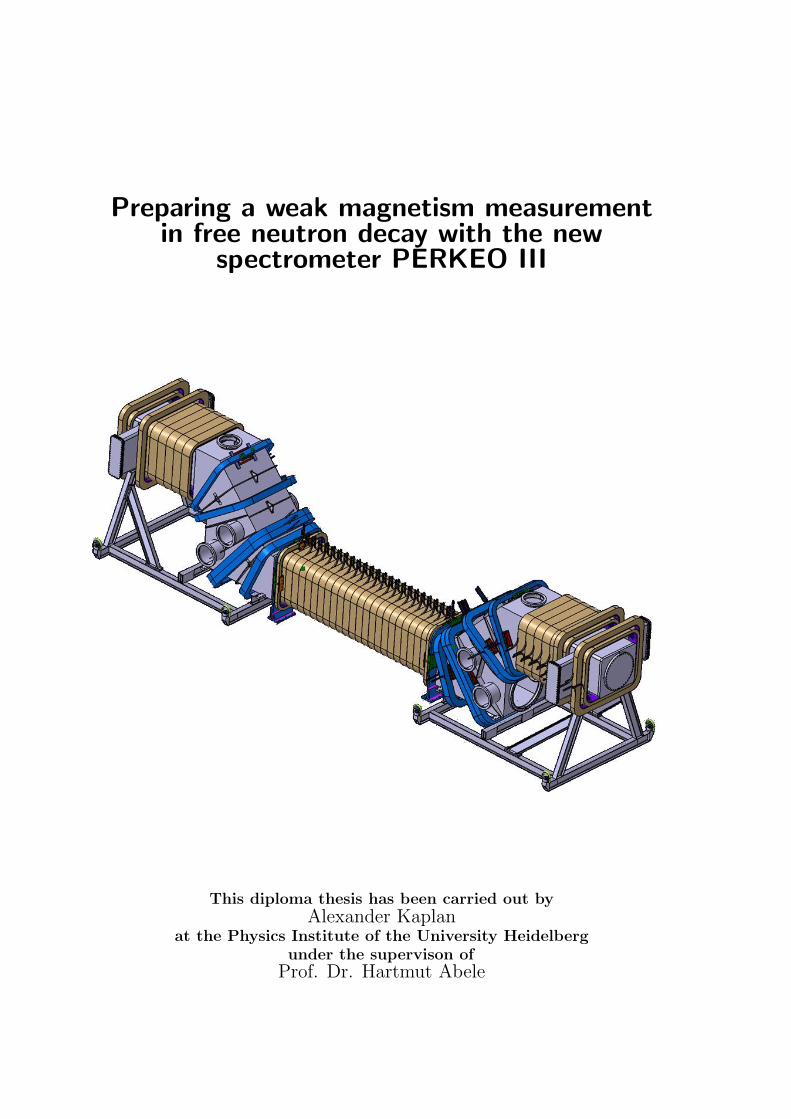
Preparing a weak magnetism measurementin free neutron decay with the new
spectrometer PERKEO III
This diploma thesis has been carried out byAlexander Kaplan
at the Physics Institute of the University Heidelbergunder the supervison of
Prof. Dr. Hartmut Abele

Alles fr den Dackel, alles fur den Club, unser Leben fur den Hund

Abstract
Preparing a weak magnetism measurement in free neutron decaywith the new spectrometer PERKEO III.
We present the preperation of the first measurement with the new spectrometer PERKEOIII: The weak magnetism form factor will be obtained from the electron asymmetry A mea-sured in the decay of free polarized neutrons. Previously, this very small energy dependenceof A was not accessible due to statical limits. For the first time ever, PERKEO III providesa neutron decay rate high enough to reach the necessary precision. It is the first of thePERKEO instruments that uses normal conducting coils to produce its magnetic field. Todissipate the heat produced by the power of 283 kW a water cooling system was developedand tested in this thesis. The data aquisition system of the predecessor PERKEO II is reusedlargely but had to be accelerated: It is now able to cope with 100 times higher data rate.During the first beam time in 2006, the instrument was installed at the cold neutron beamfacility PF1b at the Institute Laue-Langevin (ILL) in Grenoble, France. The cooling systemwas set up and works reliable, the data aquisition system was put into operation, and firstmeasurements were made.
Zusammenfassung
Vorbereitung einer Messung des Schwachen Magnetismus imZerfall freier Neutronen mit dem neuen Spektrometer PERKEO III
Wir prasentieren die Vorbereitungen der ersten Messung mit dem neuen SpektrometerPERKEO III: Der Formfaktor des Schwachen Magnetismus soll aus einer Messung der Elek-tron Asymmetrie A im Zerfall freier, polarisierter Neutronen bestimmt werden. Vorher wardiese kleine Energieabhangigkeit aus statistischen Grunden nicht zuganglich. Zum erstenMal uberhaupt wird PERKEO III eine Neutronen-Zerfallsrate zur Verfgung stellen, die großgenug ist, um die notwendige Prazision zu erreichen. Es ist das erste PERKEO Instrumentmit normalleitenden Spulen, um sein Magnetfeld zu erzeugen. Um die Warme abzufuhren, dievon 283 kW Leistung erzeugt wird, wurde im Rahmen dieser Arbeit ein Wasser-Kuhlsystementwickelt und getestet. Das Datenaufnahme-System des Vorgangers PERKEO II wird weit-gehend weiterverwendet, musste aber beschleunigt werden: Es kann nun mit den bis zu 100mal großeren Datenraten umgehen. Wahrend der ersten Strahlzeit 2006 wurde das Instru-ment am Strahlplatz fur kalte Neutronen PF1b am Institut Laue-Langevin (ILL) in Greno-ble (Frankreich) aufgebaut. Spulen-Kuhlung und Datenaufnahmesystem wurden in Betriebgenommen und arbeiten zuverlassig, und erste Messungen wurden durchgefuhrt.

Alles fr den Dackel, alles fur den Club, unser Leben fur den Hund

Contents
1. Introduction 9
2. Overview 112.1. Short Overview of Theory . . . . . . . . . . . . . . . . . . . . . . . . . . . . . 112.2. PERKEO III Overview . . . . . . . . . . . . . . . . . . . . . . . . . . . . . . 12
3. Cooling System 173.1. Fundamentals . . . . . . . . . . . . . . . . . . . . . . . . . . . . . . . . . . . . 173.2. Cooling Circulations . . . . . . . . . . . . . . . . . . . . . . . . . . . . . . . . 223.3. Waterflow Watchdog . . . . . . . . . . . . . . . . . . . . . . . . . . . . . . . . 243.4. Measurements . . . . . . . . . . . . . . . . . . . . . . . . . . . . . . . . . . . . 26
4. Data Acquisition 294.1. Overview . . . . . . . . . . . . . . . . . . . . . . . . . . . . . . . . . . . . . . 294.2. Data Rate Improvement . . . . . . . . . . . . . . . . . . . . . . . . . . . . . . 324.3. Dackel . . . . . . . . . . . . . . . . . . . . . . . . . . . . . . . . . . . . . . . . 354.4. Linearity of ADCs . . . . . . . . . . . . . . . . . . . . . . . . . . . . . . . . . 394.5. Photomultiplier Tests . . . . . . . . . . . . . . . . . . . . . . . . . . . . . . . 42
5. First Beamtime 475.1. Beam Direction . . . . . . . . . . . . . . . . . . . . . . . . . . . . . . . . . . . 475.2. Background Measurements . . . . . . . . . . . . . . . . . . . . . . . . . . . . 49
6. Summary 55
A. Time measurement in Linux using the TSC 57
7

Contents Contents
8

1. Introduction
The free neutron is an ideal object for studies on the structure weak interaction. With itslife time of approximate 15 minutes it is the instable particle with the longest life time.Sources of high neutron flux are available, allowing precision measurements with very goodstatistics. The big advantage of investigating the weak interaction with free neutrons is thatno corrections due to nuclear structure are necessary in contrast to the instable elements fromthe nuclide chart.
Over the past years, the decay of neutrons has been successfully studied by measuring corre-lation coefficients in experiments with the PERKEO instruments [Abe02, Kre05]. PERKEOIII is the latest child in this family of instruments, developed by Bastian Markisch as topic ofhis dissertation [Mar06]. It uses the same measuring principle but allows much higher eventrates, since it is much larger than its predecessors. Building up the new spectrometer andputting it into operation for a measurement of the weak magnetism coefficient is the topic ofthis diploma thesis. We obtain the weak magnetism from a small linear dependence of theelectron asymmetry in the decay of polarized neutrons. Due to the high statistics necessaryto determine such a small coefficient it was not possible to detect it in neutron decay be-fore. The experiment takes place at the high flux cold neutron facility PF1b of the InstituteLaue-Langevin (ILL), Grenoble in winter 2006 / 2007.
PERKEO III is the first of the PERKEO instruments that uses normal conducting coppercoils to generate its magnetic field. A water cooling system for the coils had to be dimen-sioned and developed which is presented in chapter 3. With the new experiment we expect adecay rate of approximate 30 kHz what made an acceleration of the existing data acquisitionsystem necessary: One subject of this thesis is the upgrade of the electronics and the devel-opment of the new data acquisition software, described in chapter 4. During the first partof the beam time, the instrument was installed and several tests concerning the shielding ofbackground radiation were done. We also examined the influence of adjacent experiments onthe background. The results are summarized in chapter 5. We begin with an overview of thetheory and the setup of PERKEO III in the next chapter.
9

CHAPTER 1. INTRODUCTION
10

2. Overview
In this chapter we give a brief overview on the theory of the neutron decay. In the secondpart, we present the spectrometer PERKEO III and the setup of the first beamtime. We alsoshow how the measured electron asymmetry Aexp is related with the weak magnetism κ.
2.1. Short Overview of Theory
The free neutron decayn → p + e− + νe (2.1)
can be seen as the prototype of the semi-leptonic weak decay of a baryon. The decay proba-bility dω with an electron energy Ee is calculated with Fermi’s Golden Rule
dω(Ee) =2π
h|Tif |2
dφ(Ee)dEe
dEe, (2.2)
where the phase space factor dφ gives the number of possible final states. The transitionmatrix
Tif ∝ JµhadrJµlept (2.3)
is proportional to the interaction of leptonic currents Jµlept and hadronic currents Jµ
hadr =Vµ
hadr + Aµhadr with
Vµhadr = 〈f | f1γµ +
i f2
mnσµνq
ν + f3qµ |i〉 (2.4)
Aµhadr = 〈f | g1γµγ5 +
i g2
2mnσµνγ
5qν + g3γ5qµ |i〉 (2.5)
The form factors f1, f2, f3, g1, g2, and g3 depend on the squared energy transfer q2 and accountfor vector, weak magnetism, induced scalar, axial vector, pseudotensor, and pseudoscalarcontributions. f3 and g2 are zero due to symmetry arguments. In the limit q2 → 0 it isf1(q2 = 0) = gV and g1(q2 = 0) = gA, where gA and gV are the axial vector and thevector coupling constants from the standard V − A formulation of the weak interaction. g3
is negligible small.For neutron β-decay, with |i〉 = |n〉 and |f〉 = |p〉, the currents read:
Jµlept = 〈e−| γµ(1− γ5) |νe〉 (2.6)
Jµhadr = 〈p| gV γµ +
i f2
mnσµνq
ν + gAγµγ5 + g3γ5qµ |n〉. (2.7)
If we calculate |Tif |2 for polarized neutrons and put it into equation 2.2, we get [Jac57]
ω = F (Ee)(
1 + apepν
EeEν+ b
me
Ee+ 〈σn〉
(A
pe
Ee+ B
pν
Eν+ D
pe × pν
EeEν
))(2.8)
11

2.2. PERKEO III OVERVIEW CHAPTER 2. OVERVIEW
for the decay probability. The neutron spin is 〈σn〉, pe and pν are the momenta of electronand neutrino and Ee, Eν are their energies. F (Ee) includes the phase-space factor φ withcorrections and the remaining factors. The β asymmetry A and the neutrino asymmetry Bare both parity violating. A triple coefficient D 6= 0 would violate time reversal invariance. bis the Fierz interference term. In V −A theory, these correlation coefficients are all functionsof λ = gA
gV, the ratio of axial vector and vector coupling constant:
a = 1−|λ|21+3|λ|2 , A = −2 |λ|
2+Re(λ)1+3|λ|2
B = 2 |λ|2−Re(λ)
1+3|λ|2 D = 2 Im(λ)1+3|λ|2
(2.9)
In equation 2.9 the asymmetry A is related to λ neglecting f2. Small energy dependentinfluences of proton recoil, weak magnetism and the gA gV interferences have to be consid-ered in precision measurements [Wil82]:
A(Ee) = A0
(1 + AµM
(A1
E0 + me
me+ A2
Ee + me
me+ A3
me
Ee + me
)). (2.10)
The uncorrected β asymmetry from equation 2.9 is labeled as A0 now. E0 = me + 782keV isthe maximum energy in neutron decay. The other factors are:
AµM = −λ+2κ+1−λ(1+λ)(1+3λ2)
memn
,
A1 = λ2 − 23λ− 1
3 ,
A2 = λ3 − 3λ2 + 53λ + 1
3 ,
A3 = 2λ2(1 + λ).
(2.11)
A1 ≈ 2.12, A2 ≈ −8.66 and A3 ≈ −0.87 are just constants for a fixed value of λ, only AµM
also depends on the weak magnetism
κ =f2(q2 = 0)f1(q2 = 0)
, (2.12)
the quantity we want to determine with the first PERKEO III measurement. κ can be relatedto the anomalous magnetic moments µa
p, µan of proton and neutron via
κ =mn
mp
µap − µa
n
2= 1.855,
hence we have a theoretical prediction for κ.
2.2. PERKEO III Overview
PERKEO III is a new spectrometer to investigate the decay of free cold polarized neutrons.It was designed to precisely measure asymmetries in the emission direction of the chargeddecay products. From the asymmetries, detailed information on the weak interaction can beextracted, such as the weak magnetism form factor described in the section above. In thissection we describe the PERKEO measuring principle, and the setup of the first PERKEOIII-beamtime to measure this factor at the ILL (Institute Laue-Langevin) in Grenoble, France.
12

CHAPTER 2. OVERVIEW 2.2. PERKEO III OVERVIEW
PERKEO measuring principle
The PERKEO measuring principle is quite simple: It makes use of a symmetric setup withtwo identical detectors. A magnetic field of 150 mT defines two hemispheres for the emissiondirection of the neutron decay products relative to the neutron spin. The field guides thecharged particles to the detectors; in this way a full 2× 2π detection is achieved, without anysolid angle corrections to be applied. Figure 2.1 schematically shows the measuring principleof PERKEO III.
Neutrons
Detector 1 Detector 2
Decay Volume
Hemisphere 1 Hemisphere 2
Neutron Spin
Figure 2.1.: PERKEO III measuring principle: Neutrons are longitudinally polarized; in thedecay volume, the spin is aligned with the magnetic field lines represented bythe blue lines. In this way, two hemispheres (in and against spin direction) aredefined. Picture by Bastian Markisch.
PERKEO III setup
In the first beamtime we want to determine the weak magnetism coefficient κ in neutrondecay from a measurement of the electron asymmetry A. The electron detectors consist eachof a large plastic scintillator (Bicron BC400) with mesh photomultiplier tubes (HamamatsuR5504), suitable to work in magnetic fields, attached on both sides, see figure 2.3.
The experiment is installed at the cold neutron beam position PF1b of the ILL. Figure 2.2shows a schematic picture of the PERKEO III setup: The neutrons leave the neutron guideH113 and pass the polarizer transmitting only neutrons with the spin in a defined direction,i.e. the beam is fully polarized afterwards. We use a supermirror polarizer and expect apolarization degree of P ≈ 98.5%, cf. [Sol02].
To compensate the different detector functions the neutron spin is flipped periodically: Aflipping by 180 degrees is equivalent to the interchange of both detectors since the magneticfield direction of the spectrometer is fixed. This is done with a radiofrequency spinflippersuccessfully used in the last PERKEO II measurements; hence we expect a spin flip efficiencyF very close to 100% [Sch04, Mun06].
The purpose of the shutter-up is to switch on and off the neutron beam. This way thebackground in the experimental hall can be measured. The beam is collimated in the beamlineto have a defined beam profile and to avoid scattering of neutrons on the instrument walls. Tomeasure the background radiation generated in the beamline, we installed a second shutter,called shutter-down. The background from the collimation can now be obtained by subtractingthe background with shutter-up closed from the background with shutter-up opened andshutter-down closed.
Behind the shutter-down the neutrons enter the decay volume. Electrons from neutrondecay generated here are guided to the detectors by the magnetic field produced by the
13

2.2. PERKEO III OVERVIEW CHAPTER 2. OVERVIEW
Figure 2.2.: Scheme of the PERKEO III setup to measure the weak magnetism. It is installedat the cold neutron beam position PF1b of the ILL.
14

CHAPTER 2. OVERVIEW 2.2. PERKEO III OVERVIEW
Figure 2.3.: PERKEO III electron detector: The plastic scintillator in the center has an areaof 43× 45 cm2 and a thickness of 0.5 cm. The scintillation light is guided to thesix photomultiplier tubes via plexiglass lightguides. In the upper part a top viewis given. Figure taken from [Mar06].
water-cooled copper coils. Neutrons that did not decay are dumped at the beamstop.
From measured data to weak magnetism
Energy and flight direction relative to the neutron spin are acquired for each detected decayelectron. From that the number electrons with energy Ee emitted in N↑(Ee) and againstN↓(Ee) neutron spin direction are obtained. This yields the experimental asymmetry
Aexp(Ee) =N↑(Ee)−N↓(Ee)N↑(Ee) + N↓(Ee)
,
that is related to the electron asymmetry A(Ee, κ), equation (2.10), via
Aexp(Ee) =12
A(Ee, κ)v
cPF,
where v is the electron velocity, P the degree of neutron polarization, and F the spinflipperefficiency. Hence one can determine the weak magnetism coefficient κ from a fit of equation(2.2) to the data.
15

2.2. PERKEO III OVERVIEW CHAPTER 2. OVERVIEW
16

3. Cooling System
The magnetic field inside PERKEO III is generated by copper coils consisting of 54 segments.It is produced by electrical currents of up to 600 A and consumes a power of 283 kW. Oncethe field is built up all the electric energy fed to the coils is transformed into thermal energyheating up PERKEO. The heat has to be dissipated to keep the coils from burning out.Therefore we developed a water cooling system pumping 160 l/min through the coils, whichare made of copper tubes for this purpose. A heat exchanger connects the cooling circulationsupplied at the ILL with the PERKEO’s own circulation.
To turn off the power supplies and the pump in case of a failure there are two independentlocking mechanisms. First, temperature switches on each single coil segment are connectedin series connection. If one of the coils heats up over 70 C its temperature switch opens theelectric circuit and the powersupplies are turned off via an interlock. As a second lockingmechanism we developed a water flow watchdog able to detect the flaking of a hose and turnoff all critical devices.
The first section of this chapter introduces some theory on fluid mechanics and thermody-namics. This is necessary to understand the calculations to dimension the cooling circulationsdiscussed in section 3.2. The water flow watchdog is presented in section 3.3. The last sec-tion shows the results of measurements that approve the correct dimensioning of the coolingsystem.
3.1. Fluid Mechanics and Thermodynamic Fundamentals
This section gives a short summary of fluid mechanics and thermodynamic fundamentals.This brief introduction derives the formulas needed for the dimensioning of the cooling system.More profound explanations can be found in [Ger77]. The empiric formulars for turbulantflow are given in [Bre03].
Waterflows
The volumetric flux is defined as Φ = v ·A with the velocity of flow v through a surface A.
Loss of pressure due to local constriction
The flux is conserved independent from any local constriction, e.g. from a pipe cross sectionA1 to a pipe cross section A2 < A1:
Φ1 = Φ2 ⇔ A1v1 = A2v2 ⇒ v2 > v1
Thus, the fluid velocity increases from v1 to v2.The energy ∆W kin = 1
2m(v22 − v1
2) = 12V ρ (v2
2 − v12) is necessary for this acceleration.
It is accomplished by a drop of pressure:
Wp1 = p1 V = p1 A1v1t
17

3.1. FUNDAMENTALS CHAPTER 3. COOLING SYSTEM
Wp2 = p2 V = p2 A2v2t
⇒ ∆W p = V (p2 − p1).
Energy conservation, ∆W kin + ∆W p = 0, leads to Bernoulli’s Equation:
p1 +12ρ v1
2 = p2 +12ρ v2
2 = const
From this it follows that every constriction leads to a pressure drop of
∆p =12
v12 ρ
[(A1
A2
)2
− 1
].
In a closed circulation there is always a return to the initial cross section. So for everyconstriction there is a dilatation an this effect cancels.
Laminar Flow
For potential flow there is no pressure drop in a tube if the cross section is constant - similar toa perfect conductor, independent of the length. However, potential water flow is completelyunphysical since it does not include real world characteristics like turbulence and friction.
Viscosity: For a thin fluid film of thickness x between a solid wall and a movable platewith an area A, the force to move the plate with a constant velocity v in parallel to the wallis
F = ηAv
x.
The property of the fluid is described by the viscosity η, which decreases strongly with growingtemperatures. For water and many other fluids the viscosity is
η = η∞ eb/T .
For water one gets η∞ ≈ 1.06 · 10−6 and b ≈ 2000 by fitting the function above to data from[Nis05], see fig. 3.1.
0.2
0.4
0.6
0.8
1.0
1.2
1.4
1.6
1.8
0 10 20 30 40 50 60 70 80 90
η[m
Pa
s]
T [C]
p = 1 barp = 5 bar
p = 10 bar
Figure 3.1.: Viscosity of water at differ-ent temperatures and pressures.The viscosity is almost com-pletely pressure independent,hence the curves at lower pres-sures are overlapped by the 10bar curve.
18

CHAPTER 3. COOLING SYSTEM 3.1. FUNDAMENTALS
.
.
dx
dy
dF2
dF1
Figure 3.2.: Frictional forces on a small volume of a fluid
Friction forces: Regarding a small volume dV = dx dy dz of a fluid streaming in y-direction and a velocity gradient in x, on the left face (see fig. 3.2) there is a frictional forceof
dF1 = −η∂v
∂x|left dy dz.
On the right face in reverse y-direction, there is a force of
dF2 = η∂v
∂x|right dy dz = η
(∂v
∂x|left +
∂2v
∂x2dx
)dy dz.
Overall on the small volume there acts a force of
dFR = dF1 + dF2 = η∂2v
∂x2dxdydz.
For the general case with velocity gradients in all directions we get
dFR = η
(∂2v
∂x2+
∂2v
∂y2+
∂2v
∂z2
)dx dy dz
= η ∆v dV.
Thus the force density is
fR =dF
dV= η4v respectively ~fR = η4~v
for an arbitrary direction of the velocity.
Forces due to pressure: A pressure gradient, e.g. along the x-axis, results in a force onthe left face of a small volume (as in fig. 3.3)
dF1 = p dy dz.
On the right face, there is also a force
dF2 = −(
p dy dz +∂p
∂xdx dy dz
).
19

3.1. FUNDAMENTALS CHAPTER 3. COOLING SYSTEM
dx
dy
dz
dF2dF1
Figure 3.3.: Forces acting on a small volume of fluid caused by pressure
The total force is
dFP = dF1 + dF2 = −∂p
∂xdV.
For arbitrary directions of the pressure gradient we get
d ~FP = −~∇p dV
and a force density of
~fP =d~F
dV= −~∇p.
Laminar flow in a tube: In a tube the fluid is at rest at the boundaries and moves withthe highest velocity at the center. On a cylinder of fluid streaming against the y-directionwith radius r and length l acts the frictional force
FR = 2πr l ηdv
dr
while on its top surface acts the pressure force
FP = πr2 (p1 − p2).
In equilibrium we have FR = FP , resulting in:
v = v0 −p1 − p2
4ηlr where v0 =
p1 − p2
4ηlR2.
R is the radius of the tube.Through a small hollow cylinder defined by the radii r and r + dr there is the volumetric
flow dV = 2πr dr v(r). For the whole tube we find the Hagen-Poiseuille law (correspondingto Ohm’s law in electricity):
V =∫ R
02πr v(r) dr =
π(p1 − p2)8ηl
R4. (3.1)
20

CHAPTER 3. COOLING SYSTEM 3.1. FUNDAMENTALS
For a tube with a constant radius R one can write the volumetric flow as V = A·v = πR2 ·v,where v is the mean streaming velocity in the tube. From this together with equation 3.1 weget the pressure drop at mean streaming velocity v:
∆p =8π
ηVl
R4= 8ηv
l
R2. (3.2)
The Reynolds Number is defined as Re = vρdη , with the density ρ of the medium and the
diameter d = 2R of the tube. Now we can write the pressure drop as:
∆p = 32η vl
d2=
32Re
v2 ρl
d= λ ρ
l
d
v2
2. (3.3)
We introduced the friction loss factor λ, which is λ = 64Re for laminar flows.
Turbulent flow : Turbulent flow or turbulence is a flow with chaotic and stochastic prop-erty changes - the opposite of laminar flow. The Reynolds number Re is an indicator whethera flow is laminar or chaotic. Flow in a tube is laminar for Re < 2000 and gets turbulent forhigher Reynolds numbers (see e.g. [Ger77, Bre03, Sto00]). The critical value of Re also de-pends on the surface of the tube. One can calculate the pressure drop for turbulent flow justas for laminar flow using equation 3.3, but with different friction loss factor λ. For straighttubes with a plain surface, one can calculate λ with empirical formulas for different ranges ofRe (see [Bre03, Sto00]):
λ =
64Re for Re < 2000
0.31644√
Refor 2000 ≤ Re ≤ 105
(3.4)
Radiation of heat
Part of the power fed to PERKEO is also dissipated by emission. To estimate the radiatedpower, we approximate the coils as black bodies. A black body with the surface area A attemperature T emits radiation of the power
P = σA T 4, (3.5)
where σ is the Stefan-Boltzmann constant σ = 5.67 · 10−8 W m−2 K−4.
Water cooling
To increase the temperature of a water mass m by ∆T , the energy
W = cw ·∆T ·m
is necessary. Under standard conditions, the specific heat capacity1 of water is cw = 4183 JKg−1 K−1 and the density is ρw = 1 g ml−1. Both can be considered constant here, sincetheir change is only about 2% in the interesting temperature range T = 10...70 C and thepressure range p = 1...10 bar - see fig. 3.4.
The other way round, if we want to dissipate the heat produced by the power P = ddtW ,
we need a water flow ofd
dtV =
1ρw
d
dtm =
1ρw
d
dt
W
cw∆T=
P
ρwcw∆T. (3.6)
1The specific heat capacity of water at constant pressure is also labeled as cp.
21

3.2. COOLING CIRCULATIONS CHAPTER 3. COOLING SYSTEM
4.17
4.18
4.19
4.20
4.21
4.22
0 10 20 30 40 50 60 70 80 90 100
T [C]
c w[J
Kg−
1K−
1]
p = 1 barp = 5 bar
p = 10 bar
0.96
0.97
0.98
0.99
1.00
0 10 20 30 40 50 60 70 80 90 100
T [C]
ρw
[gm
l−1]
p = 1 barp = 5 bar
p = 10 bar
Figure 3.4.: Specific heat capacity (left) and density (right) of water at different temperaturesand pressures, ref. [Nis05]. They both change only about 2% in in the range ofinterest (T = 10...70 C) and can be seen as constant. They can also be consideredas pressure independent.
3.2. Cooling Circulations
In this section we give an overview of the PERKEO cooling circulation. It consists of eightsubcirculations, see figure 3.5. This division has been chosen on the basis of our calculations,that are discussed in the following. The coil segments are cooled in parallel connection. Thisis physically more reasonable, since it results in higher flow and less pressure drop.
The properties of the different coil types are shown in table 3.1. The currents and windingnumbers given in the table are determined by the material properties and the desired formof the magnetic field. They have been calculated using numerical methods, refer [Mar06].From the currents and the resistances of the coil segments, one gets the electrical powerP = I · R2. We chose an uncritical temperature increase (see row “∆T” in table 3.1) andcalculated the necessary water flow (row labeled “Flow”) for each segment using equation 3.6.
The pressure drop in the cooling circulation depends on the lengths and diameters of thecoil segments and hoses, as well as on the water flow. We chose a 2 inch firehose for themain circulation and 1 inch rubber hoses for the eight subcirculations. The subcirculationsare then split up again and each single coil segment is connected with 8 mm plastic hoses.The hose materials have been chosen on the demands in pressure and temperature resistance.The hollow coil segment themselves have a diameter of 8 mm. We calculated the pressuredrop in the segments using equation 3.3, see row “∆p” in table 3.1. We also calculated thepressure drop in the 8 mm-in-diameter feed hose (see figures 3.5 and 3.6) for a length of 1 m(in row “∆p8mm”) - it is negligible, thus only the pressure drop in the coil segments is relevant.
22

CHAPTER 3. COOLING SYSTEM 3.2. COOLING CIRCULATIONS
8 mm
1"
Subcirculation 4 a/b
Subcirculation 3 a/b
Subcirculation 1 a/b
Subcirculation 2 a/b
ba
1618
12 1410
4 511
13 1519
1721
7
9
3
8
6
2
20
1
2 3
2"
1"8mm
Figure 3.5.: PERKEO III cooling system overview. The coil segments (black) and the hoseswith the distributors are shown (colored). All segments are cooled in parallel.For simplicity, only one flow direction is shown (for return direction it looksthe same). The coils are labeled with their corresponding number. Adjacentsegments belong to the same coil, if not labeled otherwise.
Coils 1 2-3 20-21 4-5 6-9 10-11 12-15 16-17 18-19Type number 22291 22292 22292 22293 22294 22295 22296 22297 22298
Number of coils 1 2 2 2 4 2 4 2 2Segmentsa 24 5 2 1 1 1 1 1 1Windingsb 8 10 10 3 5 7 6 5 6
Pliesc 3 3 3 4 6 6 6 4 6Clear height [m] 0.60 0.85 0.85 0.72 0.95 0.87 0.87 0.87 0.87Inner width [m] 0.60 0.70 0.70 0.72 0.80 0.77 1.12 0.87 0.87
Length [m]d 1525 496 198 38 116 152 155 74 137Current [A] 570 420 570 570 570 570 570 570 570
Resistance [mΩ] 301 98 39 7 24 32 32 15 28∆T [K] 22 22 22 22 29 37 38 25 31
→ V [l/min]e 2.66 2.25 4.15 1.58 3.78 3.97 3.97 2.75 4.19v [m s−1]f 0.88 0.75 1.38 0.52 1.25 1.32 1.32 0.91 1.39
Re 5346 4533 8349 3174 7612 7988 7985 5545 8443λ 0.04 0.04 0.03 0.04 0.03 0.03 0.03 0.04 0.03
→ ∆p [bar] 1.14 1.33 3.88 0.27 3.87 5.50 5.62 1.42 5.48→ ∆p8mm [bar] 0.02 0.00 0.02 0.01 0.03 0.04 0.04 0.02 0.04
a per coil b per ply c per coil segmentd conductor length (sum over all segments) e flow per segment f mean velocity
Table 3.1.: Different coil types of PERKEO III. The measures and electrical properties of thecoils are given in the upper part of the table. In the lower half the calculated flowsand the resulting pressure drops are presented.
23

3.3. WATERFLOW WATCHDOG CHAPTER 3. COOLING SYSTEM
We merged coil segments with similar pressure drops together to eight subcirculations,labeled 1a/b, 2a/b, 3a/b, 4a/b in table 3.2. Due to the symmetric structure of PERKEO III,always two subcirculations have the same pressure drop. We calculated the pressure drop inthe feeding hoses of diameter 1” - it is also negligible.
Name 1 2 3 4Coils a 1,4a 2,16 6,8,20 10,12,14,18Coils b 1,5b 3,17 7,9,21 11,13,15,19∆p [bar] 1.1 1.4 3.9 5.6
Flow [l/min] 31.9 14.0 15.9 16.1v1” [m/s] 1.05 0.46 0.52 0.53
Re1” 20207 8885 10054 10205λ1” 2.65 · 10−2 3.26 · 10−2 3.16 · 10−2 3.15 · 10−2
∆p1” [bar] 0.08 0.07 0.24 0.03
acoil 4 consits only of one segment and is connected in series with one segment of coil 1bcoil 5 consits only of one segment and is connected in series with one segment of coil 1
Table 3.2.: The eight subcirculations of the Cooling System. They are named 1a, 1b, 2a, 2b,3a, 3b, 4a, 4b. Since subcirculations with the same digit have the same properties,there are only four columns. The second and the third row are important, sincethey show how the coil segments are merged. Rows four three and four show thecorresponding water flows and pressure drops for the subcirculations. The lastfour rows contain calculated values for the 1” feed hoses of length 20m.
Assembly of the PERKEO III cooling circulation
Figure 3.6 shows the assembly of the PERKEO III cooling circulation schematically. Onlyone of the eight subcirculations is shown. The pump is connected to the first level distributor(1:8) with an 2“ firehose. From there for each subcirculation a 1” hose goes to the second leveldistributor (1:4 or 1:6), wherefrom a 8 mm hose leads to the separate coil segments. To beable to operate the subcirculations separately, the flow and the return of each subcirculationcan be shut via a gate valve. After the gate valve in the flow there is a pressure reducingregulator. In the return, in front of the gate valve, a flow meter is built in. This flow meteris part of the waterflow watchdog described in the next section.
3.3. Waterflow Watchdog
The waterflow watchdog was developed in cooperation with the electronics workshop of thePhysics Institute at the University of Heidelberg. It consists of a microcontroller box, a relaybox and eight low-cost flowmeters which are part of the PERKEO III cooling circulation.
The microcontroller box is a multipurpose device produced by the electronics workshopfeaturing a standard USB (universal serial bus) interface and a FPGA (field programmablegate array) by Xilinx as central processing unit. It can carry up to four submodules for variousapplications. The box is a stand alone device and able to run without any PC. Thanks to theFPGA it can be programmed for a wide range of tasks and new features can be implementedwithout any change of hardware.
24

CHAPTER 3. COOLING SYSTEM 3.3. WATERFLOW WATCHDOG
Dis
trib
uto
r
Dis
trib
uto
r
Distributor
Valve
Flowmeter
Valve
Fir
ehose
2"
Fir
ehose
2"
Pressure reducer
Coil segments
Hose 8mm
Hose 1"
Pump
Distributor
Figure 3.6.: Assembly of the PERKEO III cooling circulation (schematically). For simplicity,only one of the eight subcirculations is shown.
The flowmeters of type DFC.9000.100 by Parker are a precise and cheap solution for mea-suring waterflow. They can be operated within magnetic fields since the flow is measuredwith an infra-red light signal. Water passes through the sensor body impacting on a twinvaned turbine rotor, which rotates at a speed proportional to the flow rate. Two opposingphototransistors on either side of the rotor generate a continuous signal. As the rotor rotatesthe blades obscure the infrared signal which gives an industry standard pulse output signal.Its frequency is proportional to the waterflow.
The relay box is connected to the microcontroller box and the interlocks of the PERKEO IIIpower supplies and the water pump of the heat exchanger. It has eight input jacks in which thesignals from the eight flowmeters in the cooling circulation are fed in. If one of the flowmetersgives a value below a certain threshold, the relays open. This activates the interlocks and thepower supplies as well as the pump are turned off. This is achieved by frequency counters thatare compared to the flowrate. All this is implemented in the logic of the FPGA, programmedin VHDL2.
The flow limits can be set individually for each subcirculation with a LabVIEW program,which in addition allows to monitor the flows. It is also possible to give status messagesor alerts, e.g. to a mobile phone. Since the watchdog works independent of the PC, whichonly displays and logs the flow, it is not disturbed by a possible PC crash. In case of poweroutage, the relays open and all devices are turned off. This is important, since the waterflowwatchdog is on a different power supply system than the rest of PERKEO.
The functionality of the watchdog has been proven with the final setup of PERKEO atthe ILL. The switching of the interlocks worked well and was tested with different flows.Furthermore during tests of the power supplies a signal cable was removed accidently fromthe relay box, which switched off all critical devices. Figure 3.7 shows the flow in differentsubcirculations measured during operation of PERKEO at the ILL.
2VHSIC Hardware Description Language. A design entry language for electrical circuits.
25

3.4. MEASUREMENTS CHAPTER 3. COOLING SYSTEM
10
15
20
25
30
35
40
45
0 2 4 6 8 10 12 14
t [min]
Flo
w[l/m
in]
1a1b2a4a4b
Figure 3.7.: Flows in the subcircuits ofthe PERKEO III cooling systemmeasured during 15 minutes op-eration. Not all subcircuits areplotted since their curves wouldoverlap each other. In the first3.5 min the flow of the pumpwas calibrated. At t=8.2 min weturned the pump of for 0.4 min-utes.
Commercial Waterflow Switches
We also tested two commercially available waterflow switches since we expected them to bemore reliable and cheaper than a self developed solution. In our tests we monitored the waterflow with the flowmeters DFC.9000.100 by Parker to determine the switching point.
The first device tested, the SWP 114 MS from Landefeld has a mechanical functionalprinciple. The water hits onto a plate levering an adjustable magnetic switch. The adjustmentof the switching point was very imprecise as a matter of principle. We measured an inaccuracyof more than 30%. The switch flipped between its on and off state in a wide range aroundthe desired switching point, even at a constant water flow.
The second device, SWE 12/24 ES, also from Landefeld, is an electronic device using acalorimetric effect. The sensor is heated up a few degrees above the surrounding fluid. Ifthe medium flows the heat is dissipated which gives a value for the flow rate. An integratedmicrocontroller compares the flowrate to the desired values and changes the output signalwhen the rate drops below a certain limit. Again the adjustment of the switching point wasquite imprecise. The switching worked good for small flow changes, but was lost for higherchanges. We observed a strong hysteresis and a long response time of up to 20 seconds.
In summary, the investigations showed that both commercial flow switches are not sufficientfor the purpose of the PERKEO cooling system and made the development of an own solutionnecessary.
3.4. Measurements
Verification of Calculations
To check if our calculations of the cooling requirements are right and the cooling system isable to dissipate the produced heat we made test measurements. The measurements weremade with 5 coil segments (two of type 22295 and three of type 22296) cooled in parallel.The flow was measured with the DFC.9000.100 flowmeter. Table 3.3 shows the result of thetests.
The temperature increase of the coils is much less than calculated. In the calculation weassumed that all electrical power is used to heat the water. In reality only part of the poweris dissipated by water (≈ 68 - 72 %). We also calculated the power that a black body at the
26

CHAPTER 3. COOLING SYSTEM 3.4. MEASUREMENTS
temperature of the coil emits as radiation (≈ 5 - 11 %), using equation 3.5. The rest of thepower is dissipated by convection (≈ 22 %).
Our investigations show that the calculated flows are high enough to dissipate the heatfrom the copper coils.
Measurement 1 2I [A] 240 360U [V] 32 49
Pel [W] 7776 17640V [l/min] 15.2 15.2
Treturn [C] 21 28∆Tm [K] 5 12∆Tc [K] 7 17Ph [kW] 5.3 (68%) 12.7 (72%)Pe [kW] 0.8 (11%) 0.9 (5%)Pc [kW] 1.7 (21%) 4.0 (23%)
Table 3.3.: Measurement of the temperature increase of 5 coil segments, electrically seriesconnected, but cooled in parallel. The first part of the table gives the measuredelectrical parameters and the total water flow. ∆Tm is the measured, ∆Tc isthe calculated temperature increase1. The electrical power was measured withan accuracy of ±4.2%, for the temperatures we had an error of ±1 K and thewaterflow was determined with a relative error of ±1.3% In the last part thefractions of dissipated power are shown. Ph is the power used for heating thewater, Pe is emitted by a black body at Treturn and Pc is the remain, dissipatedby convection.1Provided that all electrical power is used to heat the water.
Data measured with the final PERKEO setup
Table 3.4 shows real world data measured at the ILL. The total pressure drop in the circulationwas (7.2 ± 0.1) bar. We calculated the pressure drop in the subcirculations 1a and 1b as tolow - it is two times higher than expected. We connected coils 4 and 5 in series each with another segment of coil 1, this is not taken into account in our calculations. For subcirculation3a the calculated value is very good, whereas there is a difference of 1 bar between 3a and3b. This seems to be due to different lengths of the feeding hoses.
It is important to see that equations 3.3 and 3.4 only give estimations. It is an idealizationfor straight tubes with a plain surface. The estimation for subcirculation 3a fits that wellby chance, since we did our estimations for feeding hoses of 20 m length - in reality wehave a lengths between 8 m and 16 m. We also completely ignored the pressure drop in thedistributors and valves, where turbulences are very likely. And of course we also idealized thecoil segments a straight tubes, which in reality have a lot of 90 degree bucklings. We also didnot investigate the roughness of the inner surfaces of the hoses and coil segments.
27

3.4. MEASUREMENTS CHAPTER 3. COOLING SYSTEM
Subcirculation 1a 1b 2a 2b 3a 3b 4a 4bFlow [l/min] 30.9 30.3 14.5 14.9 15.3 15.8 16.5 16.8∆pm [bar] 2.0 2.0 1.5 1.5 3.0 4.0 6.0 6.1∆pc [bar] 1.1 1.1 1.4 1.4 3.9 3.9 5.6 5.6
Table 3.4.: Real data measured during operation of Perkeo III at the ILL. Shown are theflows in several subcircuits, the measured pressure drop ∆pm and the calculatedpressure drop ∆pc. The measuring error for all pressures is ±0.1 bar, for the flowsit is ±0.1 l/min. Almost all pressure drops have been calculated as too low. Thecalculated value for subcirculation 3a fits by chance (see text for an explanation).
Summary
This is the first water cooling system ever used for a PERKEO experiment. In this firstattempt, the cooling works well and the calculations gives an order of magnitude agreement.Comparison of calculated and measured values shows that the pressure drop in the distributorsis not negligible.
28
4. Data Acquisition
In the Perkeo III experiment data acquisition consists of transformation of the scintillationlight to electric pulses, conversion to digital values and transport of the data to the measuringPC, where it is stored permanently. To control the spinflipper and calibration measurementsare also tasks of data acquisition system.
In this chapter we first give an overview of the components used. Then we present theacceleration of the data read out and introduce the new software Dackel. We also show ourinvestigations of the ADC linearity and the results of an alternative photomultiplier test.
4.1. Overview
The Aim was to reuse and improve the already available hardware of the Perkeo II experimentto handle the requirements of Perkeo III. In this section an overview of the used electroniccomponents is given including a short description of every device. Figure 4.1 shows the setupused in the experiment.
Personal Computer
For this experiment data acquisition is done with a standard PC with a 1666 MHz CPU and256 MB RAM. To reduce the risk of data loss, two new identical 300 GB harddisks wereinstalled as a level 1 software raid. As a backup system we have second a PC with exactly thesame configuration. Communication with the VME1 devices is done with the SIS 1100/3100PCI2 to VME link by Struck Innovative Systems. It consists of the SIS3100 PCI card on PCside and the SIS 1100 card on VME side.
Different Linux distributions together with different versions of the driver for the SIS devicehave been compared for performance and stability. At the time of the tests, the only driverfor Linux 2.6.x was the unofficial version 2.02. Due to inconsistencies in the Linux Kernel APIin the 2.6.x series, some additional adjustments on the driver had to be done. The differentLinux versions all showed the same performance and high stability. For the final setup wechose OpenSuSE Linux 10.1, since the latest driver version 2.04 for the SIS 3100 was testedon this Linux distribution by the Struck.
VME Devices
We use a SIS 3000 VME crate (also by Struck) for our VME components described below.
Analog to Digital Converter: An analog to digital converter (ADC) is an electronicdevice that converts continuous analog signals to discrete digital numbers. The propertiescharacterizing an ADC are introduced in section 4.4.
1Versa Module Eurocard bus. A bus standard widely used for data acquisition in physics.2Peripheral Component Interconnect. The Bus system of today’s standard PCs.
29

4.1. OVERVIEW CHAPTER 4. DATA ACQUISITION
PMT
2
PMT
3
PMT
4
PMT
5
PMT
6
PMT
1D
iscr
imin
ator
Dis
crim
inat
or
Dis
crim
inat
or
Dis
crim
inat
or
Dis
crim
inat
or
Dis
crim
inat
or
AD
C 1
AD
C 2
Delay200 ns
Coincidence Unit
AN
D
PMT
2
PMT
3
PMT
4
PMT
5
PMT
6
PMT
1D
iscr
imin
ator
Dis
crim
inat
or
Dis
crim
inat
or
Dis
crim
inat
or
Dis
crim
inat
or
Dis
crim
inat
or
Coincidence Unit
AN
D
OR
Delay200 ns
AD
C 3
AD
C 4
Cou
nter
1
Fan-
Out
not B
USY
not B
USY
Fan-
Out
TD
C C
h.1
Lat
ch B
it 1
Lat
ch B
it 3
Lat
ch B
it 4
AN
D
AN
D
OR
BU
SY 1
AD
C G
ate
BU
SY 2
AD
C G
ate
BU
SY 3
BU
SY 4
Gat
e G
ener
ator
AD
C G
ate
Glo
bal E
NA
BL
E
Glo
bal E
NA
BL
E
Tri
gger
TD
C C
h.2
Lat
ch B
it 2
Lat
ch B
it 3
Lat
ch B
it 4
BU
SY 5
Glo
bal E
nabl
eT
rigg
erT
DC
TD
C C
h.1
TD
C C
h.2
Lat
ch B
it 1
Lat
ch B
it 3
Lat
ch B
it 4
Lat
ch B
it 2
Glo
bal E
nabl
eT
rigg
erL
atch
Star
tSto
pG
loba
l Ena
ble
BU
SYBU
SY 1
BU
SY 6
BU
SY 2
BU
SY 3
BU
SY 4
BU
SY 5
BU
SY 6
BU
SY
Detector 1 Detector 2
Figure 4.1.: Schematic overview of the Perkeo III electronics
30

CHAPTER 4. DATA ACQUISITION 4.1. OVERVIEW
Figure 4.2.: The link between VME and PCI bus. Only the most important components areshown.
We use four DL642A three-channel gated integrators to measure the energy spectrum ofthe electrons from neutron decay. A capacity on each of its inputs is used to integrate overthe photomultiplier pulses. Since this way a charge Q is converted to a digital value, one alsocalls such devices QADC or QDC. The DL642A was developed at the electronic workshop ofthe Physics Institute, University of Heidelberg. Internally the DL642A is built using 14-bitADC chips, type AD7484 by Analog Devices.
Time to Digital Converter: A time to digital converter (TDC) is a device for convertinginput pulses into a digital representation of their time indices. A TDC outputs the time ofarrival for each incoming pulse. The V767A 64 channel multihit TDC by CAEN is used forPerkeo III to recognize the backscattering of electrons on the scintillators.
Latch: In digital circuits, a latch is just a particular usage of the simple flip-flop. Moregeneral, a latch is a an electronic module that stores a digital value given on its input. Wehave a SIS3600 32-bit VME Multi Event Latch by Struck to store several information of eachevent, such as spin flipper status, shutter status or which detector triggered first.
Time Counter: The time counter DL643A1 from the electronics workshop of the PhysicsInstitute is a device that saves the arrival times of incoming trigger as absolute values. Thisis realized with an internal 1 MHz clock and a 24-bit wide FIFO to store the values. Onecan see the time counter a as simple TDC. It is used to obtain an unique arrival time foreach incoming event during a measuring cycle. This way, correlations in the data caused bysystematic effects can be detected.
Digital IO: The Digital IO DL646F is another device built by the electronics workshop.It has three outputs and one input. It is used for various purposes, e.g. to control the spinflipper.
StartStop Module: The StartStop Module is a device (developed at the ILL) generatinga signal that is used to enable and disable other devices. The busy signals from the TDC,the Latch and the ADCs are fed into the StartStop Module. This way it is possible to havethe devices enabled for an exact time, with automatic compensation of the dead time.
Counters: The DL636G counters are devices that increase the value of their internalregisters when triggered. We use several counter for various purposes, such as totaling thenumber of events or determination of the dead time.
31

4.2. DATA RATE IMPROVEMENT CHAPTER 4. DATA ACQUISITION
Other Devices:
In addition to the VME devices we use many other NIM3 and one CAMAC4 module. Mostof them are fan-outs (digital and analog ones) or simple logic elements, such as digital AND,OR and NOT. Also some gate generators are used. Discriminator and the conincidence unitare both described below.
Constant Fraction Discriminator: A constant fraction discriminator is a signal pro-cessing device used to detect pulses (e.g. from scintillation detectors) with a certain pulsewidth and a characteristic rising time. It is often used, if the rising time is higher than thedesired time resolution. In this case it is impossible to use a simple threshold triggering, cf.figure 4.3.
We use the C808 16 Channel Constant Fraction Discriminator by CAEN for the CAMACbus to detect the electron signals from our photomultipliers.
t t t
Figure 4.3.: Comparison of two triggeringmethods. The trigger time isdependent on the pulse heightif simple threshold triggering isused (left). A constant frac-tion discriminator avoids this bytriggering when a certain frac-tion of the total pulse height isreached (right). Picture takenfrom [Wik06].
Coincidence Unit: A NIM-coincidence unit is used to avoid random pulses from singlephotomultipliers to be detected as an electron signal. It has several inputs and one output.The output only gives a signal if there is a signal on at least two inputs at the same timewhat suppresses random pulses efficiently.
4.2. Data Rate Improvement
For the last Perkeo II experiments (2003, 2004), data acquisition was changed from CAMACto VME, which brought a serious improvement of the deadtime, ref. [Sch04]. The maximumdata rate in these experiments was 600 Hz, including background signals. Eight ADC valueswere stored resulting in 21 bytes of information per event [Mun06], resulting in a data rateof 0.01 MB /s. For Perkeo III we expect a decay rate of approx 30 kHz. The number ofbytes per event is 40 bytes since 12 ADCs values have to be stored, so the data acquisitionsystem has to process at least 1.1 MB / s. One part of this thesis is the improvement of theexisting VME hardware to cope with the data rate increase by two magnitudes. This was
3Nuclear Instrumentation Module, a standard for electronic devices used in experimental particle and nuclearphysics.
4Computer Automated Measurement And Control - a standard bus for data acquisition and control used innuclear and particle physics and in industry.
32

CHAPTER 4. DATA ACQUISITION 4.2. DATA RATE IMPROVEMENT
achieved by using the single word DMA5 routines of the SIS3100/1100 PCI-to-VME link andimplementing new features to the existing VME devices.
In this section we first give a short introduction into the different hardware access methodsof PCs. Then we describe the SIS DMA mode and the hardware upgrades mentioned above.Finally we present the new data rates possible with the Perkeo data acquisition system.
PC Hardware access modes
In modern PCs there are several methods to transfer data between the internal devices suchas programmed input/output (PIO), interrupt driven communication and direct memory ac-cess (DMA). Here only a very brief introduction to PIO and DMA is given, necessary tounderstand how the acceleration of the data transfer was possible. More detailed informationon this topic can be found in the literature, e.g. [Rub02, Sta01].
PIO: In programmed input/output mode, all data transfered between a device and thememory has to go trough the CPU. For reading a certain amount of data words from a hard-ware device to the computer’s memory the CPU has to request each single word from thehardware. Then it has to wait until data is delivered and write it to the memory. To writingdata to a device, the same has to be done the other way round. The CPU thus is occupiedduring the data transaction and can’t do other things in the mean time.
DMA: Devices capable of direct memory access can write data directly to the computer’smemory without going the way via the CPU. The CPU only has to tell the hardware to starta data transfer and then is notified when the transfer is finished. In the mean time the CPUcan do other things, which improves performance a lot.
Today’s PCs use the PCI bus for communication between its internal components. Besidesthe more economical consumption of CPU power using the DMA mode of PCI devices hasanother big advantage: Every data transfer over the PCI bus has a certain overhead takingsome time. This overhead is due to the bus protocol, containing e.g. bus arbitration, ad-dressing, etc. In PIO mode this overhead is done for every transfered word, while in DMAmode this is done only once for a block of many data words.
VME access modes
The VMEbus architecture provides a variety of address spaces and data widths. Data transfercycles can be either single cycle or block transfer.
Single cycle mode: In single cycle mode the bus protocol (e.g. addressing) is done forevery single data word transfered. This mode can be compared to the PIO in PC data trans-fer (see above).
Block transer mode In block transfer a block of data words is transfered at once, whichavoids unnecessary overhead. This modeis similar to the DMA mode of the PC.
5Direct memory access.
33
4.2. DATA RATE IMPROVEMENT CHAPTER 4. DATA ACQUISITION
0
2
4
6
8
10
12D
ata
ragt
e[M
B/s
]
vme_A16D16_read()
vme_A16DMA_D32FIFO_read()
Figure 4.4.: Date rate comparison for the dif-ferent read out modes. The aver-age date rate for the PIO accessis 0.4 MB/s, shown on the left.On the right is the average datarate of 10.5 MB/s for the DMAaccess.
Upgrades of the VME Modules
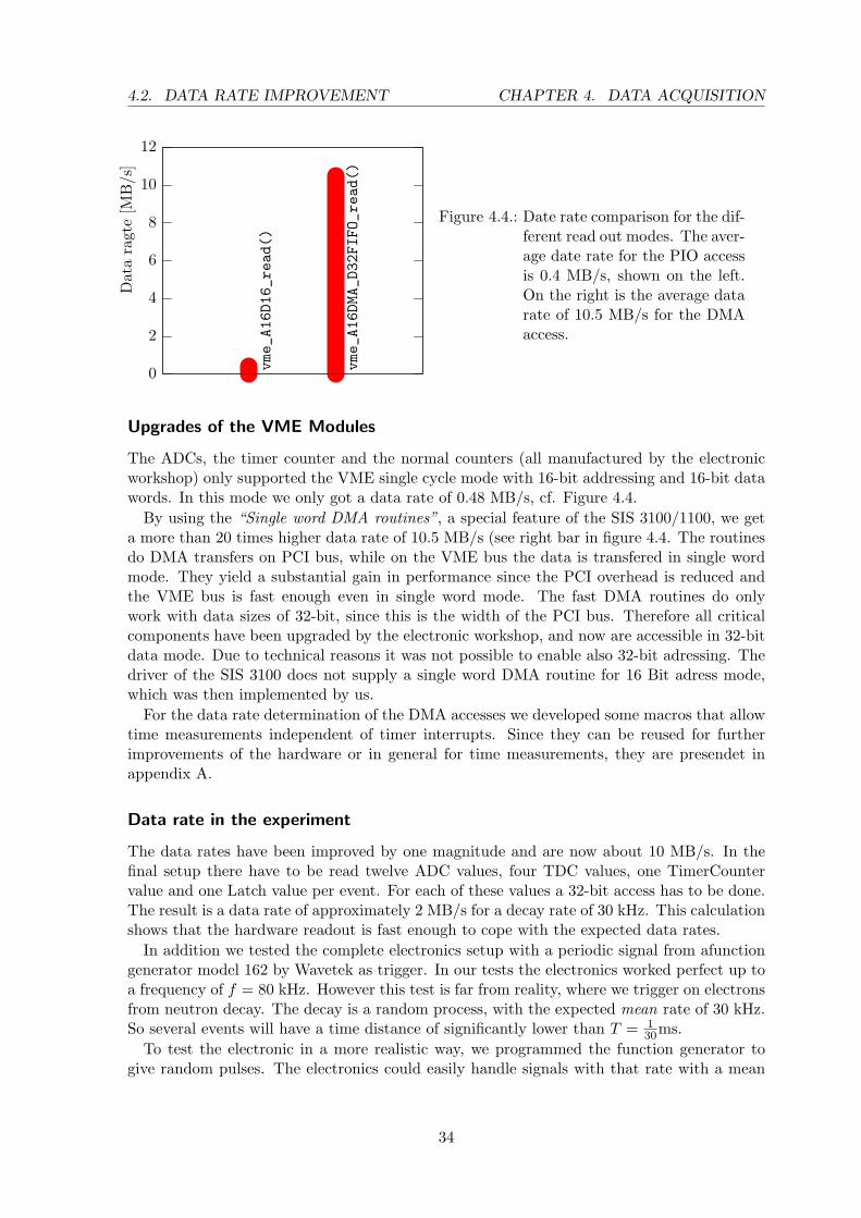
The ADCs, the timer counter and the normal counters (all manufactured by the electronicworkshop) only supported the VME single cycle mode with 16-bit addressing and 16-bit datawords. In this mode we only got a data rate of 0.48 MB/s, cf. Figure 4.4.
By using the “Single word DMA routines”, a special feature of the SIS 3100/1100, we geta more than 20 times higher data rate of 10.5 MB/s (see right bar in figure 4.4. The routinesdo DMA transfers on PCI bus, while on the VME bus the data is transfered in single wordmode. They yield a substantial gain in performance since the PCI overhead is reduced andthe VME bus is fast enough even in single word mode. The fast DMA routines do onlywork with data sizes of 32-bit, since this is the width of the PCI bus. Therefore all criticalcomponents have been upgraded by the electronic workshop, and now are accessible in 32-bitdata mode. Due to technical reasons it was not possible to enable also 32-bit adressing. Thedriver of the SIS 3100 does not supply a single word DMA routine for 16 Bit adress mode,which was then implemented by us.
For the data rate determination of the DMA accesses we developed some macros that allowtime measurements independent of timer interrupts. Since they can be reused for furtherimprovements of the hardware or in general for time measurements, they are presendet inappendix A.
Data rate in the experiment
The data rates have been improved by one magnitude and are now about 10 MB/s. In thefinal setup there have to be read twelve ADC values, four TDC values, one TimerCountervalue and one Latch value per event. For each of these values a 32-bit access has to be done.The result is a data rate of approximately 2 MB/s for a decay rate of 30 kHz. This calculationshows that the hardware readout is fast enough to cope with the expected data rates.
In addition we tested the complete electronics setup with a periodic signal from afunctiongenerator model 162 by Wavetek as trigger. In our tests the electronics worked perfect up toa frequency of f = 80 kHz. However this test is far from reality, where we trigger on electronsfrom neutron decay. The decay is a random process, with the expected mean rate of 30 kHz.So several events will have a time distance of significantly lower than T = 1
30ms.To test the electronic in a more realistic way, we programmed the function generator to
give random pulses. The electronics could easily handle signals with that rate with a mean
34

CHAPTER 4. DATA ACQUISITION 4.3. DACKEL
frequency of up 50 kHz.
4.3. Dackel
Dackel is an acronym for “Data Acquisition and Control of Electronics”. The “k” in Dackelis just a placeholder and makes the acronym easily remindable, because Dackel is also theGerman word for Teckel or Sausage Dog. Dackel is the successor of VME MOPS and the oldMOPS which are the “Measuring and Operating Systems” of PERKEO and PERKEO II.Mops is the German word for Pug, which is also a dog race, so Dackel suits well as name forthe new data acquisition system.
Since we have use the single word DMA routines described in section 4.2, it was easier towrite a new data acquisition software from scratch than try to reuse the old one. Additionally,because of the higher data rates, the use of compression is of advantage which is easier torealize when writing new code. Dackel was written in standard C++ with the GNU compilerand thus compiles on every common Linux system with installed drivers for SIS 3100.
The job of Dackel is to initialize the VME hardware, control the measurement, read themeasured data from the devices, and write it in a compressed binary format to the harddiskof the PC. Controlling the measurement means to program the StartStop card to do deadtimecompensation, start and stop the acquisition, check consistency of data and to drive the spinflipper.
In former PERKEO experiments the data aquisition program (MOPS) also controlled theshutters as well as the scanner used for calibration. Now this is done with NOMAD [Nom06],a control software of the ILL instrument control group. We enabled both software packagesto work together.
In this section the measuring scheme, the data format and its usage of Dackel are docu-mented.
Measuring scheme
In a measurement, data is taken with different configurations of the instrument which aredetermined by the states of the beam, the shutters, and the calibration scanner. For each ofthis configurations a single data file is created. Internally, a file is structured in so called cyclesthat contain the data of a certain measuring time. The duration of a cycle is adjustable, atypical value is ten seconds.
The weak magnetism form factor is calculated from the electron asymmetry in neutronβ decay. To cancel out differences between the two detectors, the spin is flipped in themeasurements (see chapter 2.2). Since part of the count rate on the detectors is alwayscaused by background radiation, linear drifts of the background would significantly distortthe asymmetry measurement. To avoid this, we use a spin flipping scheme as shown in figure4.5 which was already used in all former PERKEO experiments (see e.g. [Mun06]). SinceDackel drives the spin flipper, it also has to take care of the spin flipping scheme. For eachspin flipper state (can be on or off ), a new cycle is started. Example:
• The spin flipper is set to on.
• Wait until all neutrons that were in the beam before the flipper was changed have passedthe decay volume (which is typically some µs).
• Start measuring one cycle (typically 10 seconds).
35

4.3. DACKEL CHAPTER 4. DATA ACQUISITION
off
off
off
off
on
on
on
on
t
bac
kgro
und c
ount
rate
Figure 4.5.: Measuring scheme for the spinflipper of Perkeo III. The areabelow the line with on and offstates is equal. This way a lin-ear drift in the count rate cancelsout.
• Stop measuring
• Set spinflipper to the next state.
Usage
All options of Dackel can be set via command line parameters to enable easy instrumentcontrol using Linux shell scripts. To get the availabe parameters the program has to beinvoked in the following way:
./ dackel -h
Figure 4.6 shows the output of this invocation. Most of the options are self-explaining, suchas the setting of the VME hardware addresses. One can also set some TDC parametersexplained in [Cae01]. The time to measure is the length of one cycle, it is set via parameter-t <time> and its unit via -u <unit>. Dackel periodically reads out the buffers of the VMEdevices. For low data rates a sleep time between the read outs can be set with -s <time>.So an unnecessary polling on empty buffers is can be avoided. The compression level of thezlib routines (see [zlib]) can be set between 0 and 9 with the parameter -z <level>. If thedata acquisition system can’t handle the incoming data rate, it is a good idea to decrease thecompression level. Data is written in the format described below to the output file specifiedwith -o <file>. The pattern of the spin flipping scheme can be changed via -S <scheme>,where <scheme> is a string of 0 and 1. The scheme shown in fig. 4.5 is “10010110” forexample. Dackel waits the time given by -p <time> between the spinflips and loops over thescheme a number of times given by -l <number>.
Since most of the options do not change after the data acquisition is set up, the options canalso be written in a configuration file which is read by Dackel at startup. The configurationfile is specified via the parameter -f <file>. If no configuration file name is given, the defaultbehavior is searched in the current directory in a file named dackel.cfg.
Data Format
For each event 12 ADC values (each 16-bit), 2 TDC values (each 32-bit), one time countervalue (32-bit), and one latch value (32-bit) have to be stored. This results in 40 bytes of dataper event, corresponding to a data rate of 1.2 MB/s for the expected decay rate of 30 kHz.To reduce the necessary disk space to store the data Dackel uses a binary file format which in
36

CHAPTER 4. DATA ACQUISITION 4.3. DACKEL
------------------------------------------------------------------------------
dackel
------------------------------------------------------------------------------
usage: ./ dackel [options]
options:
-h, --help shows this help
-T, --test only show settings and exit
-f <file >, --config -file <file > use <file > as config file
ADC settings:
-A <addr >, --adc0 -addr <addr > set address of adc0 (in hex)
-B <addr >, --adc1 -addr <addr > set address of adc1 (in hex)
-C <addr >, --adc2 -addr <addr > set address of adc2 (in hex)
-D <addr >, --adc3 -addr <addr > set address of adc3 (in hex)
TDC settings:
-T <addr >, --tdc -addr <addr > set tdc address (in hex)
-E <ch#>, --tdc -channel1 <ch#> set tdc channel 1
-F <ch#>, --tdc -channel2 <ch#> set tdc channel 2
-G <tics >, --tdc -window -width <tics > set tdc window width (clock tics)
-H <tics >, --tdc -window -offset <tics > set tdc offset (clock tics)
other settings:
-U <addr >, --tc-addr <addr > set tc address (in hex format)
-L <addr >, --latch -addr <addr > set latch address (in hex format)
-I <addr >, --io-addr <addr > set io module address (in hex)
-J <addr >, --cnt1 -addr <addr > set counter1 address (in hex)
-K <addr >, --cnt2 -addr <addr > set counter2 address (in hex)
-M <addr >, --startstop -addr <addr > set startstop address (in hex)
-d <path >, --sis1100 -device <path > set sis1100 device file to <path >
-t <time >, --measure -time <time > set measure time
-u <unit >, --measure -time -unit <unit > set unit for measuretime , can be:
100ns ,1us ,10us ,100us ,1ms ,10ms ,100ms
-s <time >, --sleep -time <time > set sleep time (in us)
-z <level >, --gz-level <level > set gz compression level
-o <file >, --data -file <file > set output file
-l <file >, --log -file <file > set log file
-S <schema >, --spin -flip -schema <schema > set spin flip schema
-r <loops >, --spin -flip -loops <loops > set number of spin flip loops
-p <time >, --spin -flip -pause <time > pause between spinflips (in us)
all numbers must be given in decimal format , if not explecitly specified
Figure 4.6.: Commandline parameters of Dackel. For every option, there is a short parameter(first column) and a long parameter (second column). Some parameters requirean argument indicated by <argument>.
37

4.3. DACKEL CHAPTER 4. DATA ACQUISITION
addition is compressed with the zlib6 routines. The file consists of an uncompressed header(this is because of performance and easier programming) followed by the data for each event,see figure 4.7.
The contents of the header is shown in table 4.1. The “Magic Byte” is just a markerindicating the dkl-file format. Header length is the total length of the header in bytes. Thedate structure is explained in table 4.2. Total event count is the total number of events inthe file. Modus is a 16 bit pattern containing setup information of the measurement, seeright part of table 4.1. The field sfs_length is the length of the spin flipping scheme (whichis eight in the scheme mentioned above). sf_loop is the number of spin flips loops. Firstcycle ID is the unique identification number of the first cycle in the file. File OK is 1 ifthe measurement ended the usual way and 0 if there was an interruption. At the end of theheader an arbitrary number of counters can be saved. Per counter there is one countervaluefor each cycle.
Figure 4.7.: The file format of Dackel. Theuncompressed size of a singleevent is 40 Bytes.
DklHeader uncompressedEvent 0
.
. compressed
.Event n
Offset Description Bytes+0x0 Magic Byte 1+0x1 Version 1+0x2 Header length 4+0x6 Date (see dkl_date) 8+0xe Total event count 4
+0x12 Modus 2+0x14 Comment 256
+0x114 sfs_length 1+0x115 sf_loops 1+0x116 First cycle ID 4+0x11a Number of cycles 4+0x11e File OK 1+0x11f Number of counters 1+0x120 Counter data x
Bit Meaning10 Test9 Scan8 Source 57 Source 46 Source 35 Source 24 Source 13 Shutter-Down2 Shutter-Up1 Main Shutter0 Beam
Table 4.1.: Header structure of the .dkl-files on the left. On the right the contents of themodus field is shown.
The Event data is stored in a C-structure shown in listing 4.1. This structure is directlywritten to the outputfile via the zlib routines. To extract the compressed data to ASCIIformat the tool dkl2dat has been written. The measured data can be imported in ROOT7
with the tool dkl2root. For more detailed information refer to the source code [Dackel].
6zlib, a general purpose compression library, see [zlib] for more information.7An object-oriented data analysis framework developed at CERN, see [Root].
38
CHAPTER 4. DATA ACQUISITION 4.4. LINEARITY OF ADCS
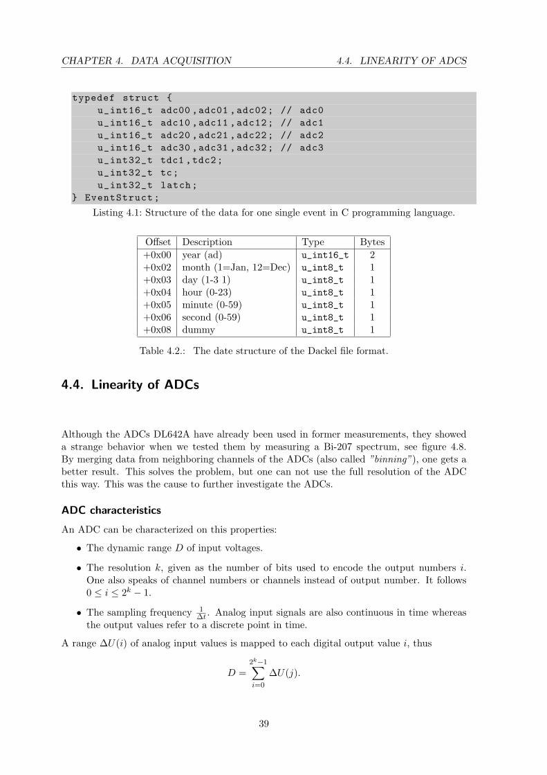
typedef struct u_int16_t adc00 ,adc01 ,adc02; // adc0u_int16_t adc10 ,adc11 ,adc12; // adc1u_int16_t adc20 ,adc21 ,adc22; // adc2u_int16_t adc30 ,adc31 ,adc32; // adc3u_int32_t tdc1 ,tdc2;u_int32_t tc;u_int32_t latch;
EventStruct;
Listing 4.1: Structure of the data for one single event in C programming language.
Offset Description Type Bytes+0x00 year (ad) u_int16_t 2+0x02 month (1=Jan, 12=Dec) u_int8_t 1+0x03 day (1-3 1) u_int8_t 1+0x04 hour (0-23) u_int8_t 1+0x05 minute (0-59) u_int8_t 1+0x06 second (0-59) u_int8_t 1+0x08 dummy u_int8_t 1
Table 4.2.: The date structure of the Dackel file format.
4.4. Linearity of ADCs
Although the ADCs DL642A have already been used in former measurements, they showeda strange behavior when we tested them by measuring a Bi-207 spectrum, see figure 4.8.By merging data from neighboring channels of the ADCs (also called ”binning”), one gets abetter result. This solves the problem, but one can not use the full resolution of the ADCthis way. This was the cause to further investigate the ADCs.
ADC characteristics
An ADC can be characterized on this properties:
• The dynamic range D of input voltages.
• The resolution k, given as the number of bits used to encode the output numbers i.One also speaks of channel numbers or channels instead of output number. It follows0 ≤ i ≤ 2k − 1.
• The sampling frequency 1∆t . Analog input signals are also continuous in time whereas
the output values refer to a discrete point in time.
A range ∆U(i) of analog input values is mapped to each digital output value i, thus
D =2k−1∑i=0
∆U(j).
39

4.4. LINEARITY OF ADCS CHAPTER 4. DATA ACQUISITION
0
10
20
30
40
50
60
70
0 4000 8000 12000 16000Channel
Num
ber
ofhi
ts
0
10
20
30
40
50
60
70
0 4000 8000 12000 16000Channel
Num
ber
ofhi
tsFigure 4.8.: Bi-207 spectrum measured with one of the ADCs before improvement of non-
linearity.
∆U is also called channel width. A perfect ADC would have a constant width for all channels.In reality all ADCs suffer from non-linearity, due to physical imperfections. That means thattheir output deviates from a linear function of their input. Their non-linearity is quantifiedby the differential non-linearity
DNL(i) =∆U(i)−∆U
∆U, (4.1)
that measures the non-constancy in width of each channel. It is of special importance forspectrum measurements, ref. [Leo94]. The integral non-linearity
INL(i) =∑
0≤j≤i
DNL(j), (4.2)
is the deviation from the linear correspondence between height of the analog input signal andthe channel number.
The integral and differential linearities are related quantities by definition, cf. equation4.2. Because the differential non-linearity for different channels can be of different sign, it ispossible that an ADC has good integral linearity, but a poor differential linearity. Thereforethe differential non-linearity is the more crucial of the two parameters. Binning cancels outthe effect of a periodic DNL, but has the disadvantage that resolution is lost.
Histogram Method to Determine the Non-Linearity
The non-linearity of an ADC can be determined with the so called histogram method, ref.[Lab]. A ramp signal covering the full dynamic range of the ADC is given as an input signal.After a large number of periods a histogram is built from the measured data. Every channel iof the ADC should have been hit approximately the same number of times N(i) ≈ N , whereN is the mean number of hits per channel. It is easy to see that the relative channel widthis equal to the relative number of hits for each channel:
∆U(i)∆U
=N(i)N
40

CHAPTER 4. DATA ACQUISITION 4.4. LINEARITY OF ADCS
The differential non-linearity then is
DNL(i) =N(i)N
− 1
Measurements
We investigated the linearity of our ADCs by applying the histogram method describedabove. We used a rampsignal with Amplitude U = 2.62V and frequency f1 = 1 Hz. The datawas sampled with a frequency of f2 = 25 kHz. Figure 4.9 (left plot) shows the differentialnon-linearity of one of our ADCs before its update done by the electronic workshop. It has astrange structure for some channels which leads to the bad spectrum in figure 4.8. By shieldingwe got rid of the effect. The shielding consists of a copper plate connected to ground thatwas glued on the body of IC8 that implements the ADC. All of our ADCs showed a similarbehavior and were thus upgraded.
After the upgrade, the differential non-linearity improved a lot, what can be seen in theright plot in fig. 4.9. In figure 4.10 the integral non-linearity before and after the upgradeare shown. Before there was a periodic structure in the integral non-linearity correspondingto the large DNL above channel 600, that vanished due to the update.
-200
0
200
400
600
800
0 4000 8000 12000 16000Channel
DN
L(i
)in
%
-200
0
200
400
600
800
0 4000 8000 12000 16000Channel
DN
L(i
)in
%
Figure 4.9.: DNL before improvement (left) and afterwards (right).
8integrated circuit
41

4.5. PHOTOMULTIPLIER TESTS CHAPTER 4. DATA ACQUISITION
0
0.2
0.4
0.6
0.8
0 4000 8000 12000 16000Channel
INL(i
)in
%
0
0.2
0.4
0.6
0.8
0 4000 8000 12000 16000Channel
INL(i
)in
%Figure 4.10.: INL before improvement (left) and afterwards (right). The integral non-linearity
is below 1% in both cases. This OK for our measurements since the dectectorcalibration is limited by other factors.
4.5. Photomultiplier Tests
The electron detector of PERKEO III consists of a large plastic scintillator (Bicron BC400)with photomultipliers (PMT for short) readout attached on two sides (see figure 2.3). ForPERKEO III we use twelve already existing mesh photomultipliers R5504 from HAMA-MATSU. These work reliable in very high magnetic fields of at least 0.5 T and alreadyproved their worth in former PERKEO experiments [Rei99, Kre04, Mun06], but are limitedin quantum efficiency. Since the PMT only needs to work in a 20 mT magnetic field in thisexperiment, we searched for less expensive standard PMTs with higher quantum efficiency asalternatives.
For this purpose the PMT 9214SB from Electron Tubes was tested, is equipped with a builtin mu-metal shield and a second external shield for operation in electromagnetic fields. Thescintillator BC400 has a maximum of emission at a wavelength of λ = 423 nm, cf. [BC400]. Atthis wavelength the quantum efficiency of the PMT 9214SB is about 27%, see [PMT9214SB].
Setup
A 5 × 5 cm2 piece of a 5 mm thick BC404 plastic scintillator was fixed to the PMT usinghigh vacuum grease. As an electron source we attached a Bi-207 conversion source directlybehind the scintillator. The Bi-spectrum has a high β-peak at 997.9 keV. The rest of thespectrum cannot be resolved due to bad energy resolution in this setup and additional gamma-background of the source, see figure 4.11. The tests were done at normal pressure of about 1bar. To generate the magnetic field we used water cooled Helmholtz coils.
Drift Test without magnetic field
The drift test was done without any additional magnetic shield, so the PMT was exposedonly to the magnetic field of the earth. We performed measurements for 15 minutes repeatedfor several hours. After an usual start-up drift within the first 2 hours, the following 19 hours
42

CHAPTER 4. DATA ACQUISITION 4.5. PHOTOMULTIPLIER TESTS
the gain stayed constant below the 1% level, cf. figure 4.11. The test was continued for 48hours, without any significant change.
0
500
1000
1500
2000
2500
3000
3500
0 50 100 150 200 250
Channel
Even
ts
15:5716:5718:5720:5822:5800:5802:5803:5804:5905:5906:5907:5908:5909:5911:14
Figure 4.11.: Drift-Test without external magnetic field. After an usual start-up drift, the Bi-207 spectrum acquired with the PMT 9214SB stays constant for several hours.
Figure 4.12.: Setup with perpendicular magnetic field.
Operation in perpendicular magnetic field
The PMT was placed inside an additional mu-metal shield MS52C (also by Electron Tubes).It was put between two coils in split pair configuration to produce a perpendicular magneticfield, see figure 4.12.
First the PMT was operated for almost 4 hours with no external field but the field of theearth. Then the magnetic field was increased up to 10 mT. As shown in figure 4.13, with
43

4.5. PHOTOMULTIPLIER TESTS CHAPTER 4. DATA ACQUISITION
the increase of the magnetic field the count rate dropped rapidly. Additionally, an hysteresiseffect occurred, since the gain is lower after the test than before (right picture in figure 4.13).
0
50
100
150
200
250
300
0 2 4 6 8 10
Magnetic Field [mT]
Count
Rate
[Hz]
0
500
1000
1500
2000
2500
3000
0 50 100 150 200 250
Channel
Even
ts
0 mT, before testsweep 1.2 and 2.2 mT
sweep 0, 3 to 10 mT0 mT, after test
constant field
Figure 4.13.: Test of the PMT 9214SB in perpendicular magnetic field. The count rate dropsrapidly with increasing magnetic field (left picture). The right graph shows theundesired change of the Bi-207 spectrum with different magnetic fields.
Test with parallel magnetic field
Although this setup is not needed for PERKEO III, we tested the behavior of the PMTparallel to the magnetic field. The result is shown in 4.14. Again, the count rate decreasedrapidly and the PMT showed an hysteresis: The gain was slightly higher after the test withthe magnetic field.
Summary
As an alternative to our existing PMTs by HAMATSU we tested the PMT 9214SB by ElectronTubes with an higher quantum efficiency compared to our standard Mesh-PMTs. Withoutany external field, there were no drifts in the gain of the PMT 9214SB. With an appliedexternal magnetic field, the performance of the PMT gets worse and in fields greater than 3mT it does not work at all.
Since the PMT 9214SB does not work properly in a magnetic field it is not sufficient forour purpose.
44

CHAPTER 4. DATA ACQUISITION 4.5. PHOTOMULTIPLIER TESTS
0
50
100
150
200
250
300
0 0.5 1 1.5 2 2.5 3 3.5 4
Magnetic Field [mT]
Count
Rate
[Hz]
0
500
1000
1500
2000
2500
3000
0 50 100 150 200 250
Channel
Even
ts
before testafter test
Figure 4.14.: Test of the PMT 9214SB in parallel magnetic field. The count rate drops withincreasing field (left). On the right the Bi-207 is shown, measured before aapplying a 3 mT field and afterwards. One can clearly see an hysteresis effect.
45

4.5. PHOTOMULTIPLIER TESTS CHAPTER 4. DATA ACQUISITION
46

5. First Beamtime
In this chapter our measurements during the first beamtime at the cold neutron beam positionPF1b at the ILL are presented. The ILL (Institut Laue-Langevin) in Grenoble, France,operates the European Neutron Source, an high flux reactor with a thermal power of 58.3MW optimized for neutron production.
5.1. Beam Direction
To install the spectrometer and the beamline at the beam position, it is necessary to knowthe beam direction. Hence we had to determine the position of the beam maximum at theend of the experimental zone wherefore we used a 3He-detector with 3% efficiency and 2× 2cm2 window, movable in horizontal (x) and vertical (y) direction, both perpendicular to thebeam.
Direct beam
First we determined the direction of the neutron beam without polarizer or any other atten-uation. This measurement was neccessary since the wall at the end of the PF1b zone wasshifted for PERKEO III by 1.5 meters; of course, the mark on the wall indicating the beamdirection was lost.
An orifice (1 mm in diameter) was fixed behind the exit of the neutron guide. We de-termined the maximum of the beam intensity in x and y−direction at the end of the zone.In x-direction, see figure 5.1, the beam profile showed an asymmetric structure due to thecharacteristics of the neutron guide, cf. [Mun00]. The origin of the small peaks at x = 500mm and x = 750 mm is unknown, maybe due to damages in the guide.
0
0.5
1
1.5
2
2.5
3
3.5
300 400 500 600 700 800 900x [mm]
Cou
ntra
tein
arbi
trar
yun
its
Figure 5.1.: Profile in x-direction of the di-rect neutron beam without po-larizer or any other attenuation,measured at the position of max-imal vertical (y) intensity. Onecan see an asymmetric struc-ture which is due to the neu-tron guide geometry. The originof the smaller peaks is unknownbut not critical for the PERKEOIII measurement.
47

5.1. BEAM DIRECTION CHAPTER 5. FIRST BEAMTIME
Polarized beam
To measure the weak magnetism form factor we need a beam of polarized neutrons. Hencea polarizer was installed directly behind the neutron guide exit. However, this deflects theneutron beam and we had to determine the beam direction again. First, the polarizer wasadjusted to gain maximum polarization by varying its angle relative to the beam.
Then we determined the beam profile with the polarizer. This time a small orifice of 5mmdiameter at the polarizer exit was used. The measured profiles are shown in figures 5.2. Inboth graphs, there is only one single peak visible, what is interesting since in some formermeasurements two or four peaks occurred. We determined the beam position at the end ofthe experimental zone from the maximum beam intensity in x and y-direction; this positionthen was used for the alignment of the beamline and the PERKEO III instrument.
Attenuated beam
In former experiments beam direction measurements were often done using plexiglass sheetsto attenuate the neutron beam for radioprotection reasons. However, it was unclear how theattenuator influences the results of the measurement. Therefore we determined the beamposition with a 10 mm plexiglas attenuator installed in front of the polarizer. As one cansee in figure 5.3 the width of the peak decreases and the maximum is slightly shifted in theattenuated measurement. Due to the decreased intensity in the attenuated case, data is scaledfor comparision. The shift of the maximum in x-direction is only a very small effect (7 mm)related to the distance between polarizer and detector (approximately 12 m).
0
2
4
6
8
10
12
0 100 200 300 400 500 600x [mm]
Cou
nts
inar
bitr
ary
unit
s
4
5
6
7
8
9
10
11
12
-100 -50 0 50 100y [mm]
Cou
nts
inar
bitr
ary
unit
s
Figure 5.2.: Beam profiles with polarizer measured at the end of the experimental zone. Left:x-profile at different y-heights (spacing 20 mm) Right: y-profile at different x-positions (spacing 20 mm). The profiles are much more symmetric and show lessstructure than figure 5.1 since a larger orifice was used and the polarizer changesthe beam divergence.
48
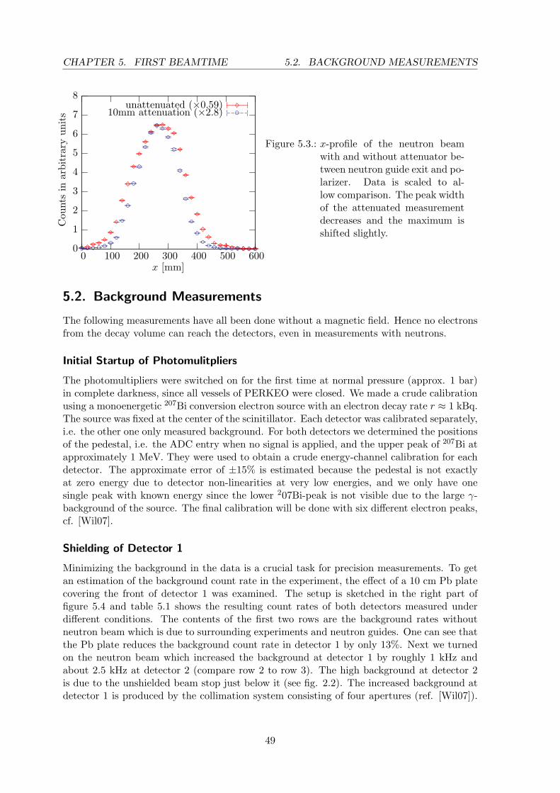
CHAPTER 5. FIRST BEAMTIME 5.2. BACKGROUND MEASUREMENTS
0
1
2
3
4
5
6
7
8
0 100 200 300 400 500 600x [mm]
Cou
nts
inar
bitr
ary
unit
s
unattenuated (×0.59)10mm attenuation (×2.8)
Figure 5.3.: x-profile of the neutron beamwith and without attenuator be-tween neutron guide exit and po-larizer. Data is scaled to al-low comparison. The peak widthof the attenuated measurementdecreases and the maximum isshifted slightly.
5.2. Background Measurements
The following measurements have all been done without a magnetic field. Hence no electronsfrom the decay volume can reach the detectors, even in measurements with neutrons.
Initial Startup of Photomulitpliers
The photomultipliers were switched on for the first time at normal pressure (approx. 1 bar)in complete darkness, since all vessels of PERKEO were closed. We made a crude calibrationusing a monoenergetic 207Bi conversion electron source with an electron decay rate r ≈ 1 kBq.The source was fixed at the center of the scinitillator. Each detector was calibrated separately,i.e. the other one only measured background. For both detectors we determined the positionsof the pedestal, i.e. the ADC entry when no signal is applied, and the upper peak of 207Bi atapproximately 1 MeV. They were used to obtain a crude energy-channel calibration for eachdetector. The approximate error of ±15% is estimated because the pedestal is not exactlyat zero energy due to detector non-linearities at very low energies, and we only have onesingle peak with known energy since the lower 207Bi-peak is not visible due to the large γ-background of the source. The final calibration will be done with six different electron peaks,cf. [Wil07].
Shielding of Detector 1
Minimizing the background in the data is a crucial task for precision measurements. To getan estimation of the background count rate in the experiment, the effect of a 10 cm Pb platecovering the front of detector 1 was examined. The setup is sketched in the right part offigure 5.4 and table 5.1 shows the resulting count rates of both detectors measured underdifferent conditions. The contents of the first two rows are the background rates withoutneutron beam which is due to surrounding experiments and neutron guides. One can see thatthe Pb plate reduces the background count rate in detector 1 by only 13%. Next we turnedon the neutron beam which increased the background at detector 1 by roughly 1 kHz andabout 2.5 kHz at detector 2 (compare row 2 to row 3). The high background at detector 2is due to the unshielded beam stop just below it (see fig. 2.2). The increased background atdetector 1 is produced by the collimation system consisting of four apertures (ref. [Wil07]).
49

5.2. BACKGROUND MEASUREMENTS CHAPTER 5. FIRST BEAMTIME
Figure 5.4.: The plot on the left shows spectra measured with the Pb plate in front of detector1. The corresponding trigger rates are shown table 5.1, row 3 and 4. Most of thebackground has an energy below 400 keV. The big difference in the detector 2rates is due to the large effect of the beamstop, that only occurs when the shutteris open. On the right, the setup with the 10 cm Pb plate is shown.
Aperture 3 for example produces around 300 Hz, what can be seen by comparing rows 3 and4 with rows 7 and 8 respectively. The closed shutter-down produces a background of 220 Hzon detector 1, which is the difference of the values in row 4 and 3, as well as row 8 and 7.
One can also see that detector 2 is not influenced by the shielding of aperture 3 and therest of the collimation system because of its distance (≈ 8 m).
Beam Shielding Shutter-up Shutter-down D1 [Hz] D2 [Hz]off none open open 415 520off Pb-plate D1 open open 360 520on Pb-plate D1 open open 1380 3050on Pb-plate D1 open closed 1600 580on none open open 2800 3040on none open closed 2960 600on Pb-plate D1a open open 1680 3070on Pb-plate D1a open closed 1900 600
aThe shielding (some Pb bricks) at aperture 3 was removed.
Table 5.1.: Influence of shielding on the background count rate measured in different setups.The two rightmost columns contain the average count rates of the two detectors.Column 3 indicates whether the Pb plate (see figure 5.4) was placed in front ofdetector 1. By calculating the differences of the several count rates one can obtainthe effects of the different configurations. This is discussed in the text.
50

CHAPTER 5. FIRST BEAMTIME 5.2. BACKGROUND MEASUREMENTS
Shielding of Detector 2
The background of detector 2 was investigated without neutron beam using again a 10 cmthick Pb plate. Two positions of the Pb plate were tested, behind detector 2 and next toit; in Figure 5.5 both configurations are shown in the picture on the right. The plot onthe left shows three spectra: one without any shielding and one for each position of theplate. One can see that in the setup with the plate next to the detector the shielding has nosignificant effect. This is interesting since a neutron guide is installed behind the wall nextto PERKEO III producing much background radiation (up to 16 µSv/h) that might disturbthe measurements. Maybe the shielding with the lead plate was not sufficient since the guideemits radiation over the whole length of the experiment.
The form of the background spectra is similar to detector 1. The Pb plate behind detector2 decreases the count rate also by roughly 13%. But in this case the background sources aredifferent: It is mainly due to the experiments directly behind our setup.
Shielding of the Beamstop
As expected, our measurements showed that a significant number of neutrons are scatteredat the 6LiF-beamstop and escape from there. To suppress their effect on the background theyhave to be shielded with boron. Therefore a cage made out of borated aliuminium (boral)will be built around the beam stop. In former measurements similiar shieldings were used,cf. [Sch04, Mun06].
Background from the Beamline
Background produced by neutrons in the beamline is crucial since it is beam related, i.e. itonly occurs when shutter-up is open. Therefore tons of lead suppressing the radiation haveto be installed around the beamline. To optimize this, several positions along the unshieldedbeamline have been investigated for γ and neutron radiation. The first was measured withthe Rados detector, a simple γ-counter available at the beam position, and the neutrons with
Figure 5.5.: Left: Three spectra acquired with detector 2 in different configurations are shown.The spectra are similar to detector 1. On the right the configuration is sketched.However, shielding detector 2 is difficult.
51
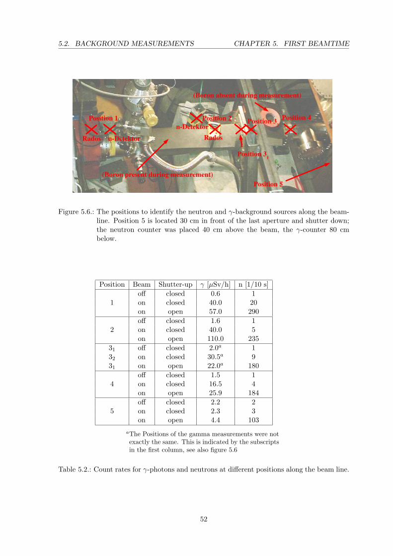
5.2. BACKGROUND MEASUREMENTS CHAPTER 5. FIRST BEAMTIME
Figure 5.6.: The positions to identify the neutron and γ-background sources along the beam-line. Position 5 is located 30 cm in front of the last aperture and shutter down;the neutron counter was placed 40 cm above the beam, the γ-counter 80 cmbelow.
Position Beam Shutter-up γ [µSv/h] n [1/10 s]off closed 0.6 1
1 on closed 40.0 20on open 57.0 290off closed 1.6 1
2 on closed 40.0 5on open 110.0 235
31 off closed 2.0a 132 on closed 30.5a 931 on open 22.0a 180
off closed 1.5 14 on closed 16.5 4
on open 25.9 184off closed 2.2 2
5 on closed 2.3 3on open 4.4 103
aThe Positions of the gamma measurements were notexactly the same. This is indicated by the subscriptsin the first column, see also figure 5.6
Table 5.2.: Count rates for γ-photons and neutrons at different positions along the beam line.
52
CHAPTER 5. FIRST BEAMTIME 5.2. BACKGROUND MEASUREMENTS
a 3He counter. Figure 5.6 indicates the different measuring positions, aperture 3 (mentionedabove) is inside the tube at position 2 of the Rados in the picture. For the investigations, weremoved its Pb brick shielding (corresponding to the measurements in row 7 and 8 in table5.1). Table 5.2 shows the count rates at the different positions without beam and with eitherof the shutters closed. One can see that aperture 3 produces much γ-radiation which agreeswith the shielding measurements above.
Background from adjacent experiments
Long time measurements of the background show structures in the count rates that are causedby experiments in the neighborhood of the PF1b beam position. By using data from INESS1 itis possible to identify some of the experiments causing this structures. This is very importantsince we later have to select data with constant background, and because wrong determinedbackground is one of the most important sources of systematic errors.
Figure 5.7 shows the background signal of both detectors and the shutter states of theneighboring experiments D1B2 and IN113. One can see that D1B only influences detector2, which is much closer to the diffractometer, whereas IN11 has a significant effect on bothdetectors.
From the data shown in figure 5.7 lower limits for the signal-to-noise ratio of rougly 5.5:1for detector 1 and 8.8:1 for detector 2 were obtained, assuming a total neutron decay rateof 30 kHz. It is only a lower limit since the test was done without any proper shielding ofbeamline and detectors.
1Service at the ILL providing the shutter status for all experiments and neutron guides.2A high intensity powder diffractometer [D1B]3Spin-Echo Spectrometer IN11 [IN11]
53

5.2. BACKGROUND MEASUREMENTS CHAPTER 5. FIRST BEAMTIME
5000
10000
15000
20000
25000
30000
0 10000 20000 30000 40000 50000 60000
t [s]
Counts
[1/10
s]
Detector 1Detector 2
D1B ShutterIN11 Shutter
Figure 5.7.: Effect of the adjacent experiments D1B and IN11 on the background count rateof the detectors. In the first 5000 seconds the neutron beam was on, then it wasswitched off and only the background of the experimental hall was measured.One can clearly identify the jumps in the count rates due to D1B and IN11.Whereas the latter can be seen in both detectors, D1B only causes an effect indetector 2.
54
6. Summary
Neutrons are an ideal object to perform precise tests of the theory of weak interaction. Theweak magnetism, a small contribution in the generalized decay matrix element accountingalso for other interaction than vector V and axialvector A, can be extracted from a energydependence of the β asymmetry A of free neutron decay. It is a very small effect in the orderof 1%. Previously this parameter was not accessible in neutron decay due to limited statistics.The new spectrometer PERKEO III is the first instrument that will achieve a neutron decayrate large enough to measure this parameter with the necessary precision.
The aim of this thesis was the preparation of the first measurement with the new instrument.It was built up at the cold neutron beam facility PF1B of the ILL.
As the first of the PERKEO instruments it uses normal conducting coils cooled with water.The high electrical power necessary to generate the magnetic field and the large number ofcoil segments require a complex cooling system with high water flow. This has been developedwithin the scope of this thesis, and the flows in the subcirculations have been calculated todimension single parts of the cooling system. A heat exchanger was installed and connectedto PERKEO and the cooling circulations at the ILL. Measurements were made to check if theheat dissipation is sufficient and the results approved that the dimensioning is correct andthat the cooling system works reliable. For safety reasons, a waterflow watchdog has beendeveloped that is able to monitor the different flows in the subcirculations and to turn off allcritical devices in case of a failure.
For the data acquisition system the electronics of PERKEO II is largely reused. Theexpected decay rate of approximate 30 kHz is two magnitudes higher than in previous exper-iments and made the acceleration of the data acquisition system necessary. To achieve this,the hardware had to be upgraded and a new readout software was written from scratch. Thesystem is now able to cope with a data rate that is 100 time higher than the data rate of thelast PERKEO II experiments. In the process of building up the electronics, the linearity ofthe used ADCs has been studied and was improved significantly.
During the first beamtime in winter 2006, first measurements were made on the beamdirection to align the spectrometer. Furthermore we started detailed studies on the beamrelated background and shielding possibilities. The influence of adjacent experiments on thebackground was examined.
55

CHAPTER 6. SUMMARY
56

A. Time measurement in Linux using the TSC
To determine and optimize the data transfer rate from the VME devices, exact time mea-surements are necessary. In a multitasking environment this is a little tricky, since severalprograms share the resources of the computer at the same time. In this appendix first isshown how the turning-off of the clock interrupt disturbed our the measurements and whythe results are wrong. Then a way how to do it right is shown. This will be useful for furtheracceleration of the data acquisition or general purpose time measurements in Linux.
Our first approach to measure the data rate was by using the POSIX1 clock() function,shown in listing A.1. The constant CLOCKS_PER_SEC equals 1000000, hence on a 32-bit systemthe function returns the same value every 72 minutes. The problem of this method are wrongresults if the clock interrupt is turned off during the measurement. This gives a far to lowtime difference, which leads to the wrong results. This is the case for the SIS3100/1100 DMAtransfers invoked by vme_A32DMA_D32FIFO_read(), see figure A.1. The average time perrequest and the data rate are completely unrealistic for this function.
t1 = clock //save time before action
action (); //do action to measure
t2 = clock(); //save time after action
// calculate the difference and scale it to secondsdt = (t2 -t1) / CLOCKS_PER_SEC;
Listing A.1: First approach to measure the data rate of the VME system.
To get proper results one has to use a different method. Most modern processors havean internal register counting the CPU cycles, it is called Time Stamp Counter (TSC). Thiscounter is incremented on every cycle the CPU does. Our system has CPU frequency of 1.6GHz, so we achieve a resolution of 0.625 ns.
The TSC method also has some problems:
• To calculate a measured time value the CPU frequency has to be known.
• On some modern processors, the frequency is not constant to save energy.
• A 32-bit wide TSC overflows in few seconds for CPU frequency in the order of 1 GHz.
• The read out of a 64-bit TSC is not possible as a single access, but may not be inter-rupted for correct measurement.
In our 32-bit Linux environment the TSC can be read out via the macro rdtsc(), ref[Rub02]. The macro takes care that no interruption occurs during read out of the 64-bit
1Portable Operating System Interface for uniX - a family of standards by the IEEE for compatibility withUnix operating systems.
57

APPENDIX A. TIME MEASUREMENT IN LINUX USING THE TSC
0
1
2
3
4
5
6
Aver
age
tim
eper
reques
t[µ
s]
vme_A16D16_read()
vme_A16DMA_D16FIFO_read()
vme_A32DMA_D32FIFO_read()
vme_A32D32_read()
vme_A32D16_read()
s3100_control_read()
0.1
1
10
100
Aver
age
data
rate
[MB
/s]
vme_A16D16_read()
vme_A16DMA_D16FIFO_read()
vme_A32DMA_D32FIFO_read()
vme_A32D32_read()
vme_A32D16_read()
s3100_control_read()
Figure A.1.: First time measurements for different requests to the VME Bus using theSIS3100/1100 PCI to VME link. The values for vme_A32DMA_D32FIFO_read()are wrong. This can be seen from the unrealistic values for request durationand data rage (the standard VME bus is maximally capable of 40 MB/s datarate). The timer interrupt used for the measurements is turned off during DMA-accesses to the PCI bus. This givs far to low time differences and leads to thewrong results.
TSC. We can easily figure out the cpu frequency, which is constant for our system. A work-around for a non-constant cpu frequency is given in [Kun06]. We developed some macrosthat make the time measurements very easy:
• TM_INIT() figures out the cpu frequency and has to be called only once in the program.
• TM_START() must be called just before the action to measure starts.
• TM_STOP() ends the measurement. It handles possible overflows and calculates the timeelapsed.
Listing A.2 shows the source code of the macros:
#ifndef timemeasure_h#define timemeasure_h
#include <stdlib.h>#include <string.h>#include <stdio.h>
#include <asm/msr.h>
#ifdef __cplusplusextern "C" #endif
u_int32_t tm_cpu_freq;
58
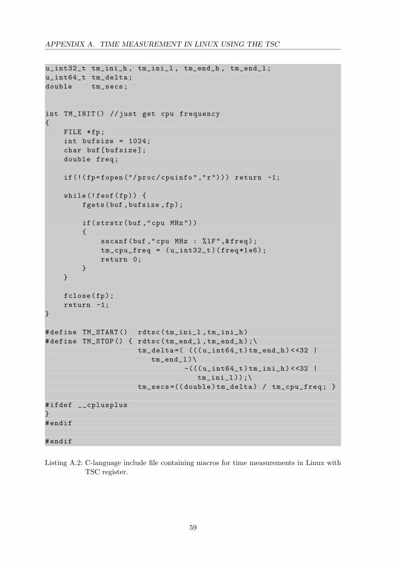
APPENDIX A. TIME MEASUREMENT IN LINUX USING THE TSC
u_int32_t tm_ini_h , tm_ini_l , tm_end_h , tm_end_l;u_int64_t tm_delta;double tm_secs;
int TM_INIT () //just get cpu frequency
FILE *fp;int bufsize = 1024;char buf[bufsize ];double freq;
if(!(fp=fopen ("/ proc/cpuinfo","r"))) return -1;
while (!feof(fp)) fgets(buf ,bufsize ,fp);
if(strstr(buf ,"cpu MHz"))
sscanf(buf ,"cpu MHz : %lF",&freq);tm_cpu_freq = (u_int32_t)(freq*1e6);return 0;
fclose(fp);return -1;
#define TM_START () rdtsc(tm_ini_l ,tm_ini_h)#define TM_STOP () rdtsc(tm_end_l ,tm_end_h);\
tm_delta =( ((( u_int64_t)tm_end_h) <<32 |tm_end_l)\
-((( u_int64_t)tm_ini_h) <<32 |tm_ini_l));\
tm_secs =(( double)tm_delta) / tm_cpu_freq;
#ifdef __cplusplus#endif
#endif
Listing A.2: C-language include file containing macros for time measurements in Linux withTSC register.
59

APPENDIX A. TIME MEASUREMENT IN LINUX USING THE TSC
An example for usage of the macros define above is given in listing A.3
#include "timemeasure.h"
int main(int argc ,char *argv [])
int i,j,k;double mean =0;
if( TM_INIT () ) return -1; // error on init , exit program
for(k=0; k <10000; k++) TM_START ();for(i=0; i <100; i++)
j=i*i;TM_STOP ();
mean += tm_secs * 1000;printf ("cpu frequency = %d [Hz]\n\n"
"the action took %g [ms]\n\n", tm_cpu_freq ,mean /10000);
return 0;
Listing A.3: Example how to use the macros for a time measurement. The first 100 squarenumber are calculated. To increase the accuracy, the measurement is repeated10000 times.
60

Bibliography
[Abe02] H. Abele et al., Phys. Rev. Let. 88 (2002) 21
[BC400] Data sheet for Bicron BC400 Premium Plastic Scintillators,available from http://www.detectors.saint-gobain.com
[Bre03] A. Brehm, Praktikum der Technischen Chemie, Stromungslehre, 2003http://www.uni-oldenburg.de/tchemie/Praktikum/Stroemungslehre.pdf
[Cae01] CAEN: Technical Information Manual TDC V767A, 2001 http://www.caen.it/getattach.php?mod=V767A&obj=mn
[Dackel] Dackel source code available from: http://www.physi.uni-heidelberg.de/∼kaplan/dackel
[D1B] High intensity powder diffractometer D1B at ILL, http://www.ill.fr/YellowBook/D1B/
[Ger77] H.Vogel, Gerthsen Physik, z.B. 13. Auflage, 1977
[IN11] Spin-Echo Spectrometer IN11, http://www.ill.fr/YellowBook/IN11/
[Jac57] J.Jackson, S.Treiman and H.Wyld, Jr.: Possible Tests of Time Reversal Invariancein Beta Decay. In: Phys. Rev., 106 (1957) 517-521.
[Kun06] Kunst, Quade: ”Kerntechnik”, Folge 27, Linux Magazin 04/06, S.118http://www.linux-magazin.de/Service/Books/Buecher/HW-Treiber/book1.html
[Kre04] M. Kreuz: Messung von Winkelkorrelationen im Zerfall polarisierter Neutronen mitdem Spektrometer PERKEO II, Ph.D. thesis 2004
[Kre05] M. Kreuz, Phys. Lett. B 619 (2005) 263
[Lab] Labcourse Computer Science, Kirchhoff Institute for Physics,Unit3: Basics of Analog Digital Converters, Manualhttp://www.kip.uni-heidelberg.de/ti/teaching/labcourse/unit3/
[Leo94] W.R. Leo, Techniques for Nuclear and Particle Physics Experimens, 2nd Edition,1994
[Mar06] B.Markisch: Das Spektrometer Perkeo III und der Zerfall des freien Neutrons, Ph.D.thesis 2006
[Mun00] D.Mund: Aufbau eines Experiments zur Messung der Neutrinoasymetrie im Zerfallfreier Neutronen, Dipl. thesis 2000
[Mun06] D.Mund: Messung der Beta-Asymmetrie A im Neutronenzerfall, Ph.D. thesis 2006
61

Bibliography Bibliography
[Nis05] E.W. Lemmon, M.O. McLinden and D.G. Friend, ”Thermophysical Properties ofFluid Systems” in NIST Chemistry WebBook, NIST Standard Reference Database Num-ber 69, Eds. P.J. Linstrom and W.G. Mallard, June 2005, National Institute of Standardsand Technology, Gaithersburg MD, 20899 (http://webbook.nist.gov).
[Nom06] NOMAD: www.ill.fr/pages/science/User/pdf/NOMAD.pdf
[Plo00] C.Plonka: Verbesserung der Lichtauskopplung zur Messung der Neutrinoasymetriemit Perkeo II, dipl. thesis 2000
[PMT9214SB] Data sheet for Electron Tubes PMT 9214SB,http://www.electrontubes.com/pdf/9214B.pdf
[Rei99] J.Reich: Winkelkorrelationen im Zerfall polarisierter Neutronen, Ph.D. thesis 1999
[Root] ROOT: An object-oriented data analysis framwork developed at CERNhttp://root.cern.ch
[Rub02] Rubini, Corbert: Linux-Geratetreiber, Kapitel 3, 2. Auflage, 2002
[Sch04] M.Schumann: Probing the Standard Model: Preparation of a new Electron AsymetryMeasurement in the Decay of Polarized Neutrons, Diploma thesis 2004
[Sch07] M.Schumann: Ph.D. thesis in progress 2007
[Sta01] W. Stallings: Operating Systems, 2001
[Sto00] H.Stocker: Taschenbuch der Physik, 4. Auflage, 2000
[Sol02] T.Soldner, A.Petoukhov, C.Plonka: Installation and first tests of the new PF1b po-lariser, 2002
[Wil82] D. H. Wilkinson: Analysis of neutron β-decay. In: Nuclear Physics A, 337 (1982)474-504
[Wil07] D.Wilkin: Diploma thesis in progress, 2007
[Wik06] Wikipedia: picture of a signal in a constant fraction discriminator.
[zlib] zlib general purpose compression library http://www.zlib.net/
62

Erklarung:
Ich versichere, dass ich diese Arbeit selbstandig verfasst und keine anderen als die angegebenenQuellen und Hilfsmittel benutzt habe.
Heidelberg, den 12. Januar 2007


![arXiv:0906.2789v6 [stat.AP] 2 Jun 2013Boudewijn F. Roukema Torun´ Centre for Astronomy, Faculty of Physics, Astronomy and Informatics, Nicolaus Copernicus University, ul. Gagarina](https://img.pdfslide.net/doc/110x75/60592592a093b371ad71a099/arxiv09062789v6-statap-2-jun-2013-boudewijn-f-roukema-torun-centre-for-astronomy.jpg)