Embed Size (px)
Citation preview
FACULTY OF SCIENCE AND TECHNOLOGY
MASTER’S THESIS
Study program/specialization:
Offshore Technology/ Subsea and Marine
Technology
Spring semester, 2018
Open
Writer: Mikhail Chumikov
.................................
(Writer’s signature)
Faculty supervisor: Professor Ove Tobias Gudmestad
External supervisor: Professor Anatoly Borisovich Zolotukhin
Title of thesis: Subsea Template Lifting Operations in the Sea of Okhotsk
Credits (ECTS): 30
Key words: marine operations, weather
window, icing
Pages: 51
Enclosure: 6
Stavanger, June 14th, 2018
2
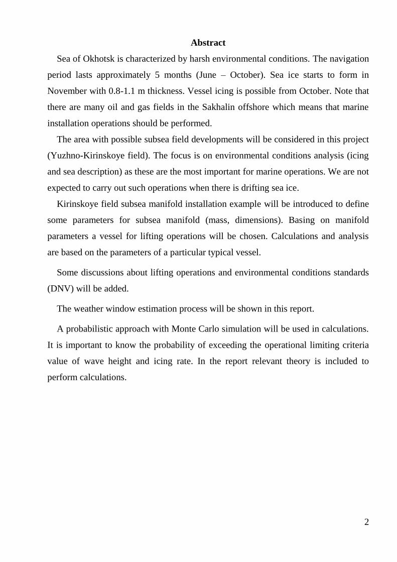
Abstract
Sea of Okhotsk is characterized by harsh environmental conditions. The navigation
period lasts approximately 5 months (June – October). Sea ice starts to form in
November with 0.8-1.1 m thickness. Vessel icing is possible from October. Note that
there are many oil and gas fields in the Sakhalin offshore which means that marine
installation operations should be performed.
The area with possible subsea field developments will be considered in this project
(Yuzhno-Kirinskoye field). The focus is on environmental conditions analysis (icing
and sea description) as these are the most important for marine operations. We are not
expected to carry out such operations when there is drifting sea ice.
Kirinskoye field subsea manifold installation example will be introduced to define
some parameters for subsea manifold (mass, dimensions). Basing on manifold
parameters a vessel for lifting operations will be chosen. Calculations and analysis
are based on the parameters of a particular typical vessel.
Some discussions about lifting operations and environmental conditions standards
(DNV) will be added.
The weather window estimation process will be shown in this report.
A probabilistic approach with Monte Carlo simulation will be used in calculations.
It is important to know the probability of exceeding the operational limiting criteria
value of wave height and icing rate. In the report relevant theory is included to
perform calculations.
Acknowledgement
I would like to thank Professor Ove Tobias Gudmestad, Professor Anatoly
Borisovich Zolotukhin and Professor Mirzoev Dilizhan Allakhverdievich for their
consultation, support and valuable advices.
I appreciate that Stanislav Duplensky, Evgeny Pribytkov and Elena Skokova have
found the time to give me useful information, which was included in the Master’s
Thesis.
Valuable consultation during the meeting in MRTS JSC office was given by
Mikhail Balyka and Stanislav Nesterenko. The meeting was organised with the help
of Anatoly Zolotukhin and Ekaterina Poelueva.
Table of Contents
Abstract.......................................................................................................................... 2
Acknowledgement ......................................................................................................... 3
List of Abbreviations ..................................................................................................... 6
List of Figures ............................................................................................................... 7
List of Tables ................................................................................................................. 9
1. Introduction ........................................................................................................... 10
2. Lifting Operation Area .......................................................................................... 14
2.1. The Sakhalin Shelf and the Sea of Okhotsk ................................................ 14
2.2. Meteorological Conditions .......................................................................... 17
3. Template and Vessel Selection ............................................................................. 19
3.1. Template Structure ...................................................................................... 19
3.2. Offshore Construction Vessel...................................................................... 22
4. Short Term Sea Description .................................................................................. 24
5. Duration of Marine Operation .............................................................................. 26
6. Weather Restricted and Weather Unrestricted Operations ................................... 28
7. Operational Limiting Environmental Criteria ....................................................... 29
8. Weather Window .................................................................................................. 32
8.1. Weather Forecast ......................................................................................... 35
9. Probability of Exceeding the Operational Environmental Limiting Criteria ....... 37
10. Icing ................................................................................................................... 41
11. Ice Growth Calculation ...................................................................................... 45
12. Discussions ........................................................................................................ 47
12.1. Weather Window Estimation ...................................................................... 47
5
12.2. Calculated Probability of Exceedance icing-rate value ............................... 47
13. Conclusion ......................................................................................................... 48
References ................................................................................................................... 49
Appendix A ................................................................................................................. 52
Appendix B .................................................................................................................. 54
Appendix C .................................................................................................................. 55
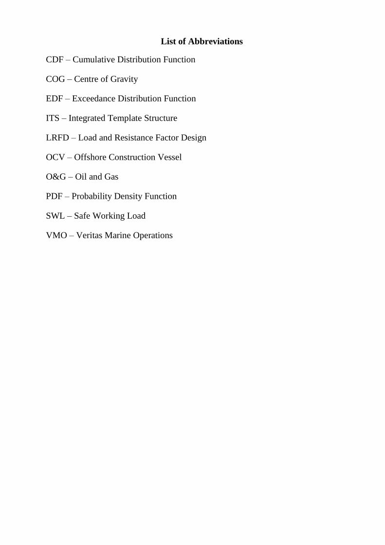
List of Abbreviations
CDF – Cumulative Distribution Function
COG – Centre of Gravity
EDF – Exceedance Distribution Function
ITS – Integrated Template Structure
LRFD – Load and Resistance Factor Design
OCV – Offshore Construction Vessel
O&G – Oil and Gas
PDF – Probability Density Function
SWL – Safe Working Load
VMO – Veritas Marine Operations
List of Figures
Figure 1 – Kirinskoye Field [1]
Figure 2 - Sakhalin Shelf Projects [3]
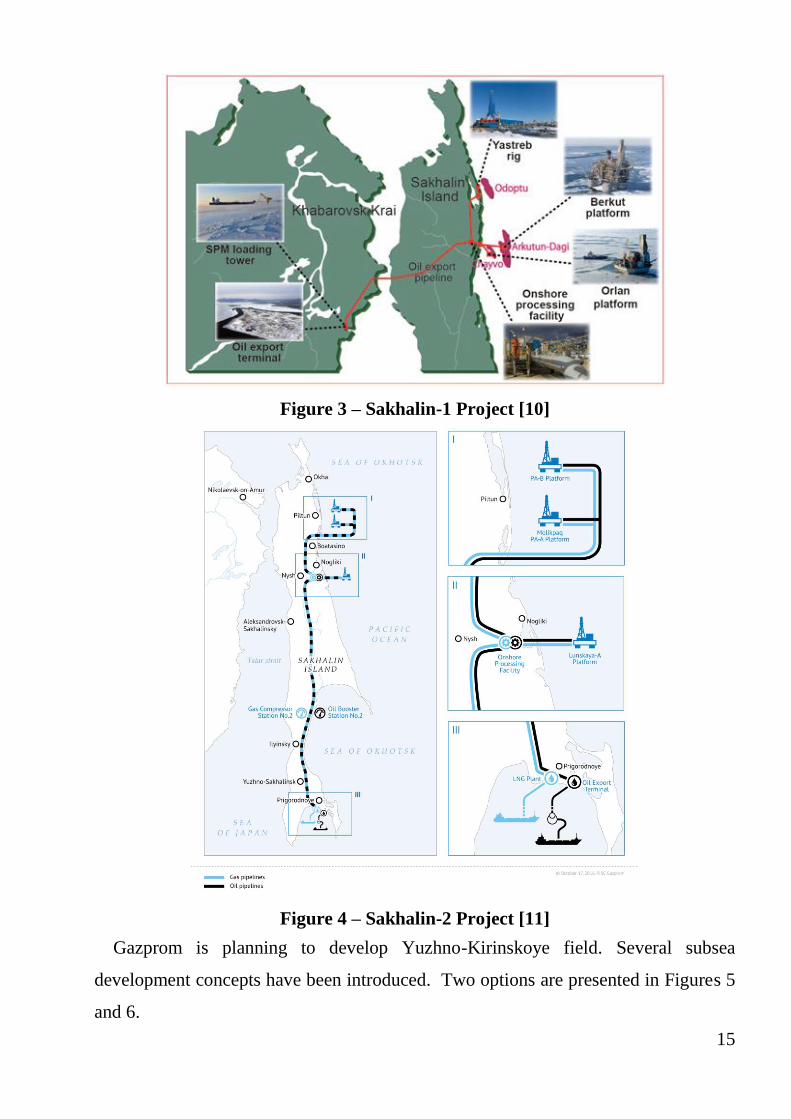
Figure 3 – Sakhalin-1 Project [10]
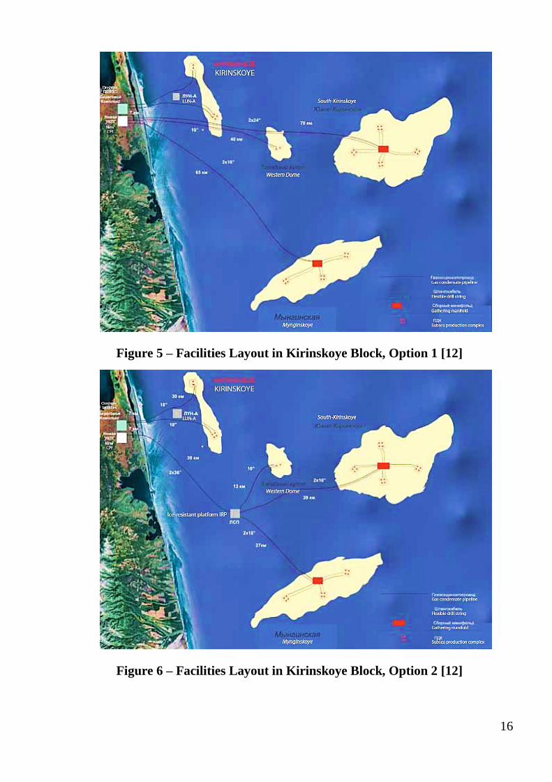
Figure 4 – Sakhalin-2 Project [11]
Figure 5 – Facilities Layout in Kirinskoye Block, Option 1 [12]
Figure 6 – Facilities Layout in Kirinskoye Block, Option 2 [12]
Figure 7 – Marked Point for Meteorological Data Extraction [14]
Figure 8 – Minimum (green), Maximum (red) and Mean (blue) Temperature (0C)
during a Year [14]
Figure 9 - Minimum (green), Maximum (red) and Mean (blue) Wind Speed (m/s)
during a Year [14]
Figure 10 - Minimum (green), Maximum (red) and Mean (blue) Wave Height (m)
during a Year [14]
Figure 11 – Kirinskoye Field Layout [17]
Figure 12 – Kirinskoye Subsea Manifold [17]
Figure 13 – Kirinskoye Subsea Manifold Lift off [4]
Figure 14 – OCV “Normand Oceanic” [18]
Figure 15 – “Normand Oceanic” vessel specification [18]
Figure 16 – Determination Procedure of Weather Restricted and Weather
Unrestricted Operations [7]
Figure 17 – Load Chart Example [22]
Figure 18 - Operation Periods [6]
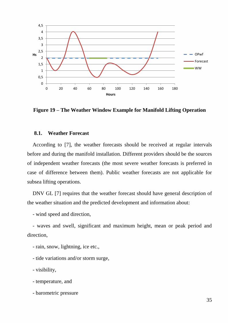
Figure 19 – The Weather Window Example for Manifold Lifting Operation
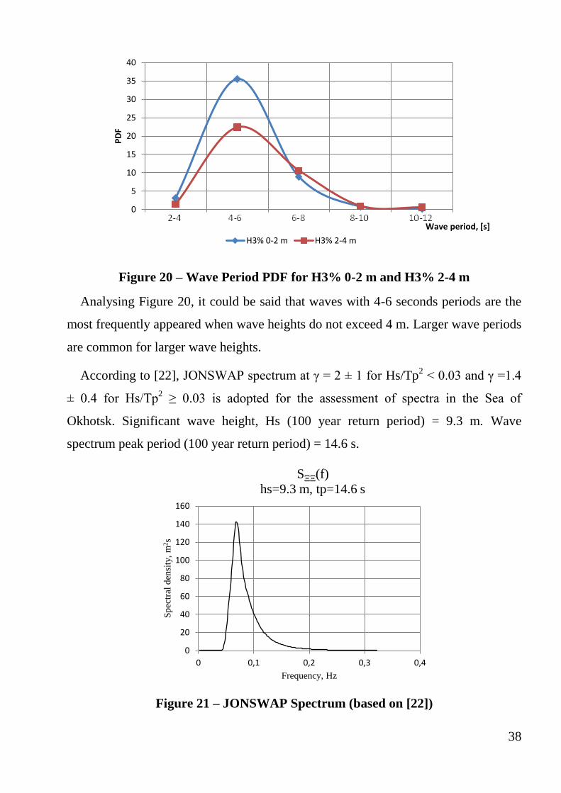
Figure 20 – Wave Period PDF for H3% 0-2 m and H3% 2-4 m
8
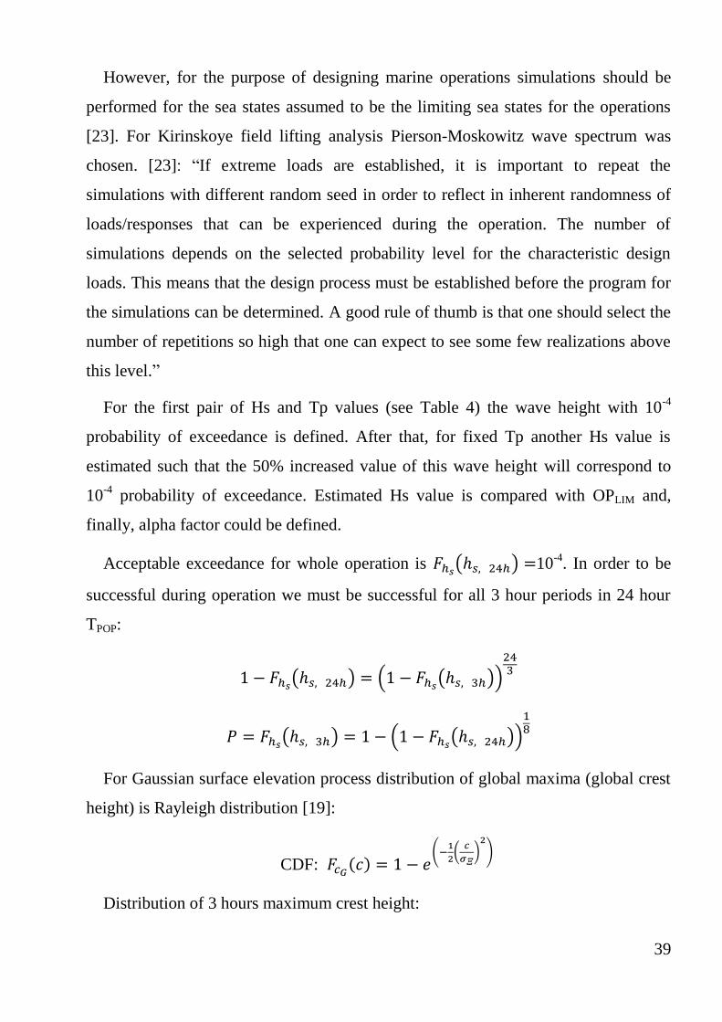
Figure 21 – JONSWAP Spectrum (based on [22])
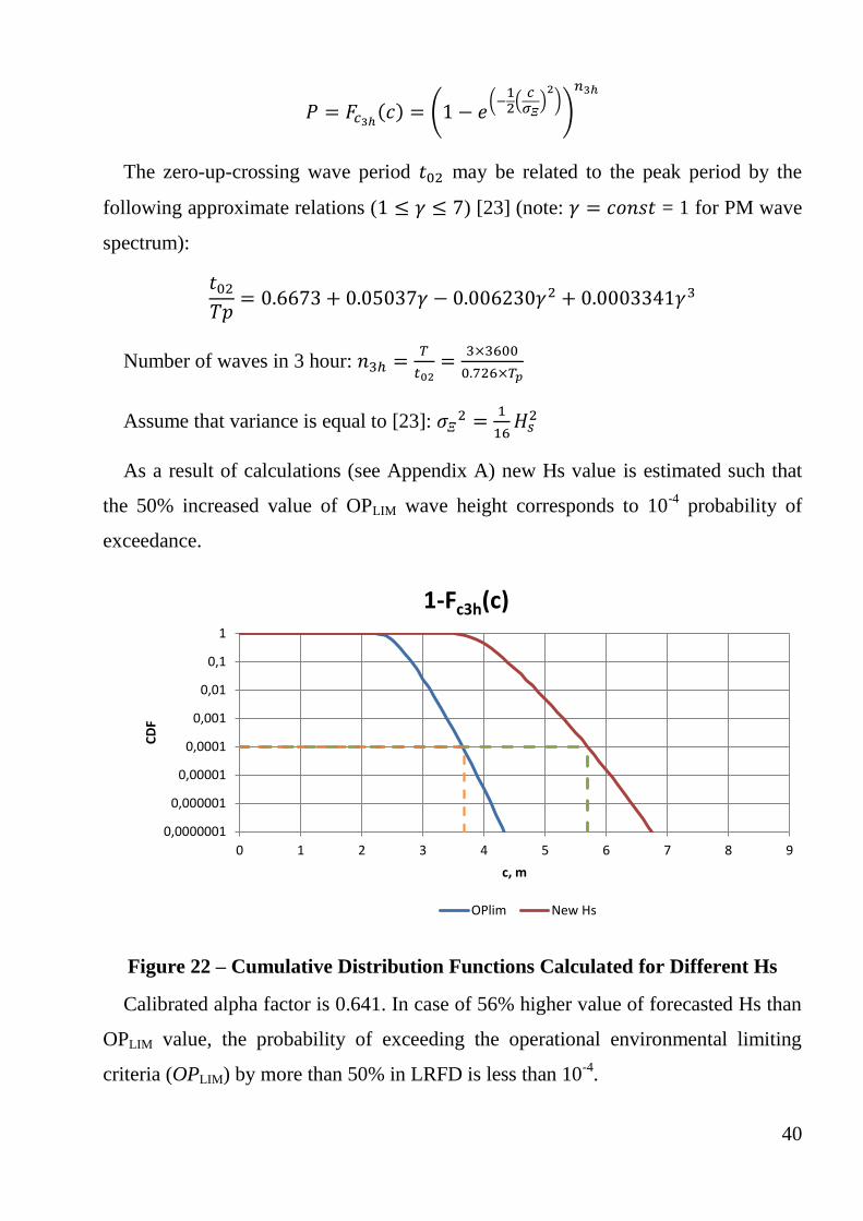
Figure 22 – Cumulative Distribution Functions Calculated for Different Hs
Figure 23 – Wet Icing. Heat Fluxes (continuous spray) [24]
Figure 24 – Ice Growth Probability Density Function
Figure 25 - CDF of Ice Growth
Figure 26 - Estimation of 7 mm/hr Probability of Exceedance
List of Tables
Table 1 – Sakhalin Oil and Gas Industry Overview
Table 2 – Comparison of Kirinskoye and Yuzhno-Kirinskoye Fields
Table 3 – Simulations Procedure [4]
Table 4 – Example of maximum Hs and Tp
Table 5 – Weather Forecast Levels [7]
Table 6 - LRFD Alpha Factor for waves, Level A2 or B – No Environmental
Monitoring [7]
Table 7 - Operational Criteria (OPWF) Estimation
Table 8 – Joint Distribution of H3% and Wave Period for ice-free period [23]
Table 9 – Icing-rate Severity Categories [25]
1. Introduction
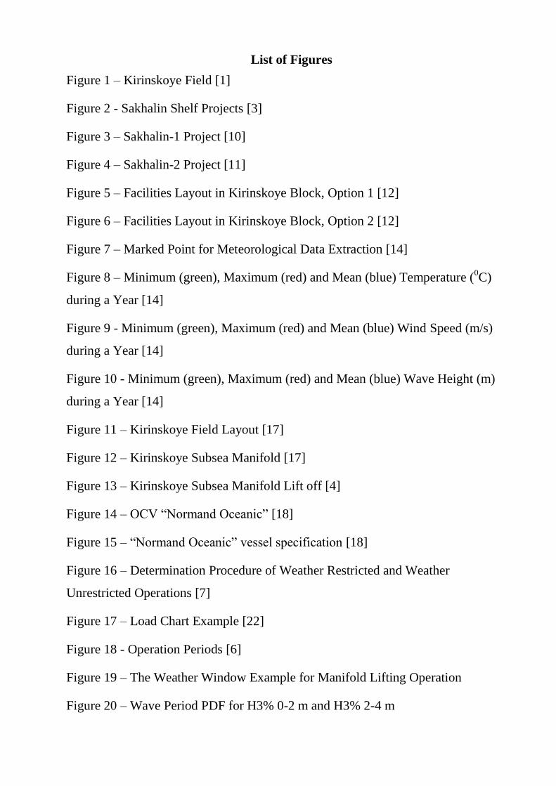
Several discoveries have been made on Sakhalin Island Shelf which attract the
O&G companies. Some of the fields require subsea development due to deep waters
and sea ice drifting. Kirinskoye field which is tied-back to shore is operating today
(Figure 1).
Figure 1 – Kirinskoye Field [1]
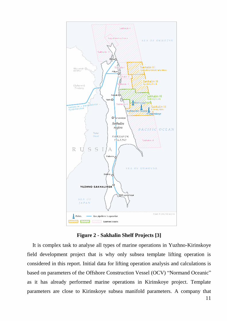
Future marine operations will be performed on another field in “Sakhalin 3”
project as Gazprom is planning to develop Yuzhno-Kirinskoye field [2]. (Figure 2).
11
Figure 2 - Sakhalin Shelf Projects [3]
It is complex task to analyse all types of marine operations in Yuzhno-Kirinskoye
field development project that is why only subsea template lifting operation is
considered in this report. Initial data for lifting operation analysis and calculations is
based on parameters of the Offshore Construction Vessel (OCV) “Normand Oceanic”
as it has already performed marine operations in Kirinskoye project. Template
parameters are close to Kirinskoye subsea manifold parameters. A company that
12
needs to install subsea templates should be doing this in a safe way and with
minimum risk. For instance, in Kirinskoye development project the analysis of
manifold installation was based on DNV “VMO Standard” Part 2-5 [4], [5].
However, general information about requirements and recommendations for
planning, preparations and performance of marine operations was given in DNV-OS-
H101 [6]. Currently, DNVGL-ST-N001 [7] replaces the legacy DNV-OS-H-series.
Sea of Okhotsk is characterized by harsh environmental conditions. Estimation of
exceeding the operational limits is carried out in this report as it is essential to define
the risk of appearance of undesirable conditions. There are some important natural
phenomena that have an impact on marine operations such as [6], [7]:
wind;
waves;
current;
tides.
Some environmental conditions also should be considered in marine operations
design:
sea ice;
icing;
temperature;
fog etc.
The navigation period in the Sea of Okhotsk lasts approximately 5 months (June –
October). Sea ice starts to form in November. Vessel icing is possible from October.
In case of large scope of work installation vessels could be on site during icing
period. This natural phenomenon does not lead to extremely dangerous conditions,
especially on large vessels, but could decrease a safety level on board. According to
[7], vessel icing should be considered in planning and execution of marine
operations. This report includes explanation of icing mechanism and icing rate
calculation procedure.
13
Subsea template installation is not a difficult operation which requires a very small
significant wave height. Usually after onshore preparations the installation vessel
goes to the installation area. The weather window should be longer than required time
for installation to perform the lifting operation. The weather window estimation
process will be shown in this report. Following LRFD calibrated alpha factor will be
estimated.
2. Lifting Operation Area
The subsea template lifting operation which is considered in this report is referring
to the Sakhalin Island Shelf. Sufficient depth and optimal conditions for subsea
development are available for the development of the Yuzhno-Kirinskoye field,
which is 6 km from the Kirinskoye field to the Southeast.
2.1. The Sakhalin Shelf and the Sea of Okhotsk
Harsh environmental conditions are the main feature of Sakhalin Island and the
Sea of Okhotsk. Sea ice drifting, low temperature, winds and waves, seismic activity,
tsunami are typical phenomena for this region [8].
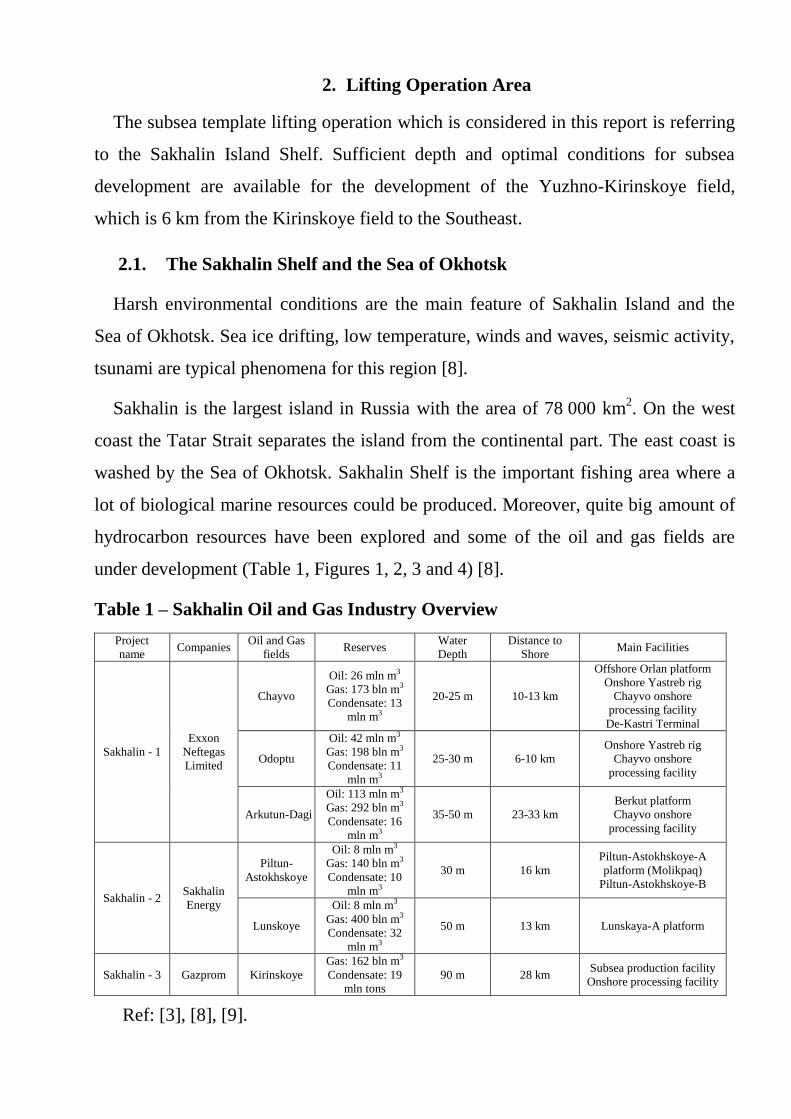
Sakhalin is the largest island in Russia with the area of 78 000 km2. On the west
coast the Tatar Strait separates the island from the continental part. The east coast is
washed by the Sea of Okhotsk. Sakhalin Shelf is the important fishing area where a
lot of biological marine resources could be produced. Moreover, quite big amount of
hydrocarbon resources have been explored and some of the oil and gas fields are
under development (Table 1, Figures 1, 2, 3 and 4) [8].
Table 1 – Sakhalin Oil and Gas Industry Overview
Project
name Companies
Oil and Gas
fields Reserves
Water
Depth
Distance to
Shore Main Facilities
Sakhalin - 1
Exxon
Neftegas
Limited
Chayvo
Oil: 26 mln m3
Gas: 173 bln m3
Condensate: 13
mln m3
20-25 m 10-13 km
Offshore Orlan platform
Onshore Yastreb rig
Chayvo onshore
processing facility
De-Kastri Terminal
Odoptu
Oil: 42 mln m3
Gas: 198 bln m3
Condensate: 11
mln m3
25-30 m 6-10 km
Onshore Yastreb rig
Chayvo onshore
processing facility
Arkutun-Dagi
Oil: 113 mln m3
Gas: 292 bln m3
Condensate: 16
mln m3
35-50 m 23-33 km
Berkut platform
Chayvo onshore
processing facility
Sakhalin - 2 Sakhalin
Energy
Piltun-
Astokhskoye
Oil: 8 mln m3
Gas: 140 bln m3
Condensate: 10
mln m3
30 m 16 km
Piltun-Astokhskoye-A
platform (Molikpaq)
Piltun-Astokhskoye-B
Lunskoye
Oil: 8 mln m3
Gas: 400 bln m3
Condensate: 32
mln m3
50 m 13 km Lunskaya-A platform
Sakhalin - 3 Gazprom Kirinskoye
Gas: 162 bln m3
Condensate: 19
mln tons
90 m 28 km Subsea production facility
Onshore processing facility
Ref: [3], [8], [9].
15
Figure 3 – Sakhalin-1 Project [10]
Figure 4 – Sakhalin-2 Project [11]
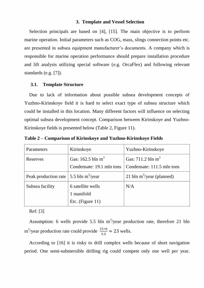
Gazprom is planning to develop Yuzhno-Kirinskoye field. Several subsea
development concepts have been introduced. Two options are presented in Figures 5
and 6.
16
Figure 5 – Facilities Layout in Kirinskoye Block, Option 1 [12]
Figure 6 – Facilities Layout in Kirinskoye Block, Option 2 [12]

17
Yuzhno-Kirinskoye С1+С2 reserves (Russian system of reserves classification)
amount is 711.2 bln m3 of gas, 111.5 mln tons of gas condensate (recoverable) and
4.1 mln tons of oil (recoverable). The water depth changes from 110 m to 320 m. [3]
2.2. Meteorological Conditions
Sea of Okhotsk is considered as Sub-Arctic sea. Close location to the cold of the
Siberian pole and development of the Siberian High results in harsh winters.
However, small effect of tropical cyclones and Soya current contribute to mild
summer climate. [13]
Temperature, wind speed and wave height distributions near Yuzhno-Kirinskoye
field location (Figure 7) are shown on Figures 8, 9 and 10.
Figure 7 – Marked Point for Meteorological Data Extraction [14]
Figure 8 – Minimum (green), Maximum (red) and Mean (blue) Temperature
(0C) during a Year [14]

18
Figure 9 - Minimum (green), Maximum (red) and Mean (blue) Wind Speed
(m/s) during a Year [14]
Figure 10 - Minimum (green), Maximum (red) and Mean (blue) Wave Height
(m) during a Year [14]
3. Template and Vessel Selection
Selection principals are based on [4], [15]. The main objective is to perform
marine operation. Initial parameters such as COG, mass, slings connection points etc.
are presented in subsea equipment manufacturer’s documents. A company which is
responsible for marine operation performance should prepare installation procedure
and lift analysis utilizing special software (e.g. OrcaFlex) and following relevant
standards (e.g. [7]).
3.1. Template Structure
Due to lack of information about possible subsea development concepts of
Yuzhno-Kirinskoye field it is hard to select exact type of subsea structure which
could be installed in this location. Many different factors will influence on selecting
optimal subsea development concept. Comparison between Kirinskoye and Yuzhno-
Kirinskoye fields is presented below (Table 2, Figure 11).
Table 2 – Comparison of Kirinskoye and Yuzhno-Kirinskoye Fields
Parameters Kirinskoye Yuzhno-Kirinskoye
Reserves Gas: 162.5 bln m3
Condensate: 19.1 mln tons
Gas: 711.2 bln m3
Condensate: 111.5 mln tons
Peak production rate 5.5 bln m3/year 21 bln m
3/year (planned)
Subsea facility 6 satellite wells
1 manifold
Etc. (Figure 11)
N/A
Ref: [3]
Assumption: 6 wells provide 5.5 bln m3/year production rate, therefore 21 bln
m3/year production rate could provide
21∗6
5.5≈ 23 wells.
According to [16] it is risky to drill complex wells because of short navigation
period. One semi-submersible drilling rig could compete only one well per year.

20
Consequently, to reduce complexity it is better to use satellite wells or 4-slots
Integrated Template Structure (ITS).
Figure 11 – Kirinskoye Field Layout [17]
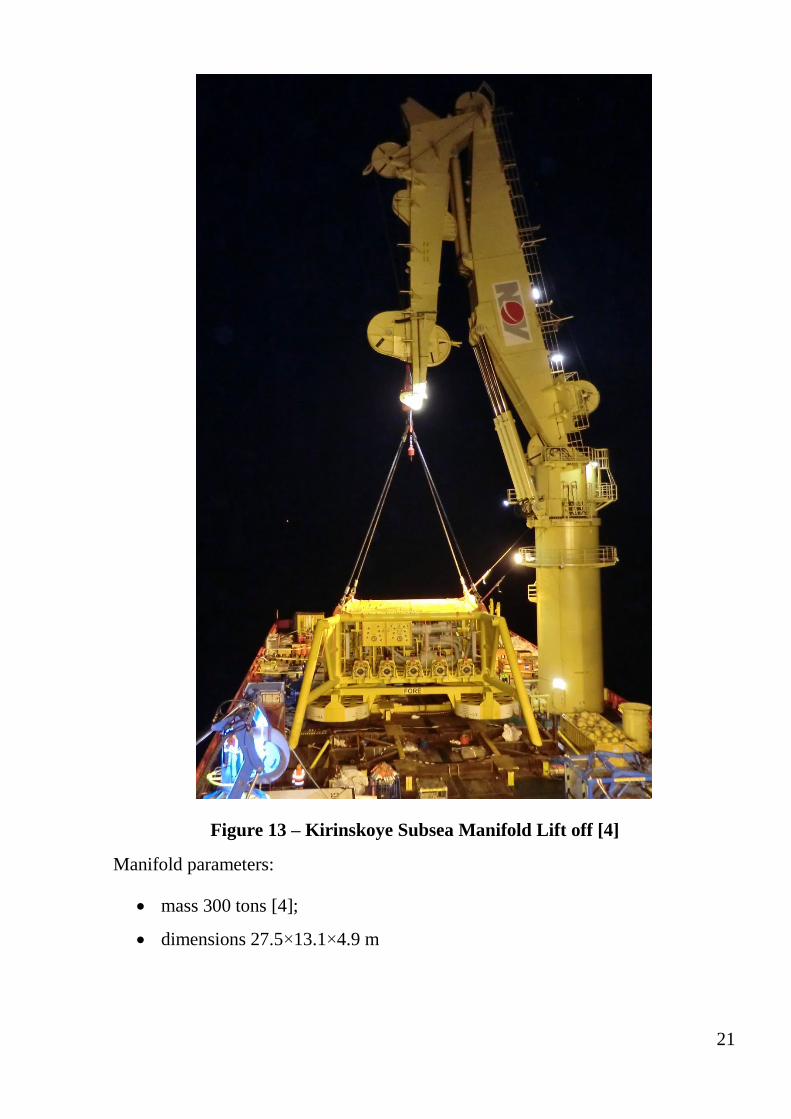
Such parameters as mass, length, width and height of ITS, piles’ length etc. depend
on specific field data. As an example, template structure with pre-installed manifold
having the same mass and dimensions as Kirinskoye subsea manifold is taken (Figure
12, 13).
Figure 12 – Kirinskoye Subsea Manifold [17]
21
Figure 13 – Kirinskoye Subsea Manifold Lift off [4]
Manifold parameters:
mass 300 tons [4];
dimensions 27.5×13.1×4.9 m

22
3.2. Offshore Construction Vessel
300 tons manifold lifting operation considered in this report. “Normand Oceanic”
vessel (the owner is Subsea 7) could perform this operation as the main crane Safe
Working Load (SWL) is 400 tons and in addition active heave compensation system
make it possible to operate in higher values of significant wave height Hs (Figure 14
and 15).
Figure 14 – OCV “Normand Oceanic” [18]
Figure 15 – “Normand Oceanic” vessel specification [18]
23
Lift analysis should be carried out before performing marine operation. Companies
should follow required standards to perform safe marine operations. For example, in
2011 when subsea manifold was installed in Kirinskoye field location companies
followed DNV-OS-H205 [5]. DNVGL-ST-N001 [7] has replaced legacy DNV-OS-
H-series standards.
4. Short Term Sea Description
Important theory of sea description is based on [19].
Solution of linearized governing equations (i.e. boundary equations are applied at
the mean free surface and first order terms are considered):
𝜉(𝑥, 𝑡) = 𝜉0sin(𝜔𝑡 − 𝑘𝑥)
It is a sinusoidal wave but real waves do not look like this (except swell). They are
less regular.
Assume that sea surface repeats after time T. Applying Fourier analysis the sea
surface could be described as the sum of sinusoidal waves:
𝜉(𝑡) = ∑(𝑎𝑛 cos2𝜋𝑛
𝑇𝑡 + 𝑏𝑛 sin
2𝜋𝑛
𝑇𝑡)
∞
𝑛=1
If 𝜉𝑛 = √𝑎𝑛2 + 𝑏𝑛
2 and 𝜃𝑛 = 𝑎𝑟𝑐𝑡𝑎𝑛 (𝑏𝑛
𝑎𝑛) sum transformed to:
𝜉(𝑡) = ∑ 𝜉𝑛cos(𝜔𝑛𝑡 − 𝜃𝑛)∞𝑛=1 .
Assume phase as a random variable uniformly distributed between 0 and 2π:
𝛯(𝑡) = ∑ 𝜉𝑛cos(𝜔𝑛𝑡 − 𝛩𝑛)∞𝑛=1
In order to obtain one realization of Ξ(t), N different phases could be generated,
Θn, n=1, …, N.
Ξ(t) is a sum of a lot of independent random components. None of the components
dominate hence according to the central limit theorem:
𝑓𝛯(𝜉, 𝑡) =1
√2𝜋𝜎𝛯(𝑡)𝑒−1
2(
𝜉
𝜎𝛯(𝑡))2
– Ξt is Gaussian (normal) probability distribution.
Description of a short term sea state:
Wave spectrum, SΞΞ(f).
Spectral moments: 𝑚𝛯,𝑛 = ∫ 𝑓𝑛𝑆𝛯𝛯(𝑓)𝑑𝑓∞
0
Variance of surface process: 𝜎𝛯2 = 𝑚𝛯,0 = ∫ 𝑆𝛯𝛯(𝑓)𝑑𝑓
∞
0
25
Expected frequency between zero-up-crossing 𝑓0̅2 = √𝑚𝛯,2
𝑚𝛯,0 and average period
between zero-up-crossing 𝑡0̅2 =1
𝑓0̅2
Expected number of global waves in time T: 𝑛𝑇 = 𝑇𝑓0̅2
5. Duration of Marine Operation
According to [7], the duration of marine operations could be defined by an
operation reference period, TR (see Figure 6): TR = TPOP + TC
where
TR = Operation reference period;
TPOP = Planned operation period;
TC = Estimated maximum contingency time.
The planned operation period (TPOP) should normally be based on a detailed
schedule for the operation.
Typical subsea template (ITS) lifting operation times are as follows [15]:
- Launch ROV and survey location - 2 h
- Connect lift rigging to template and remove sea fastening - 1h
- Overboard and deploy template - 4 h
- Orientate template by ROV or flying clump weight - 1 hr
- Land template, confirm position - 3 h
- Complete and confirm suction penetration of the structure - 24 h
- Overboard and install guide posts - 6 h
- Install template hatches - 8 h
- Overboard manifold - 1 h
- Deploy and land manifold on template - 2 h
- Recover rigging and ROVs - 2h
Planned operation period on Kirinskoye field was 24 h. Scope of work [4]:
Set-up over installation location;
ROV preparation and deployment;
Survey of location, preparation of ROV tools;
27
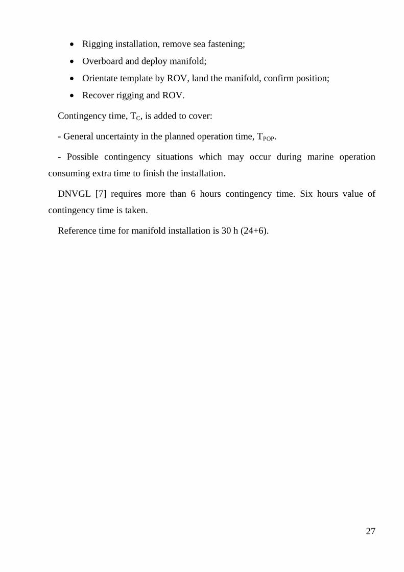
Rigging installation, remove sea fastening;
Overboard and deploy manifold;
Orientate template by ROV, land the manifold, confirm position;
Recover rigging and ROV.
Contingency time, TC, is added to cover:
- General uncertainty in the planned operation time, TPOP.
- Possible contingency situations which may occur during marine operation
consuming extra time to finish the installation.
DNVGL [7] requires more than 6 hours contingency time. Six hours value of
contingency time is taken.
Reference time for manifold installation is 30 h (24+6).
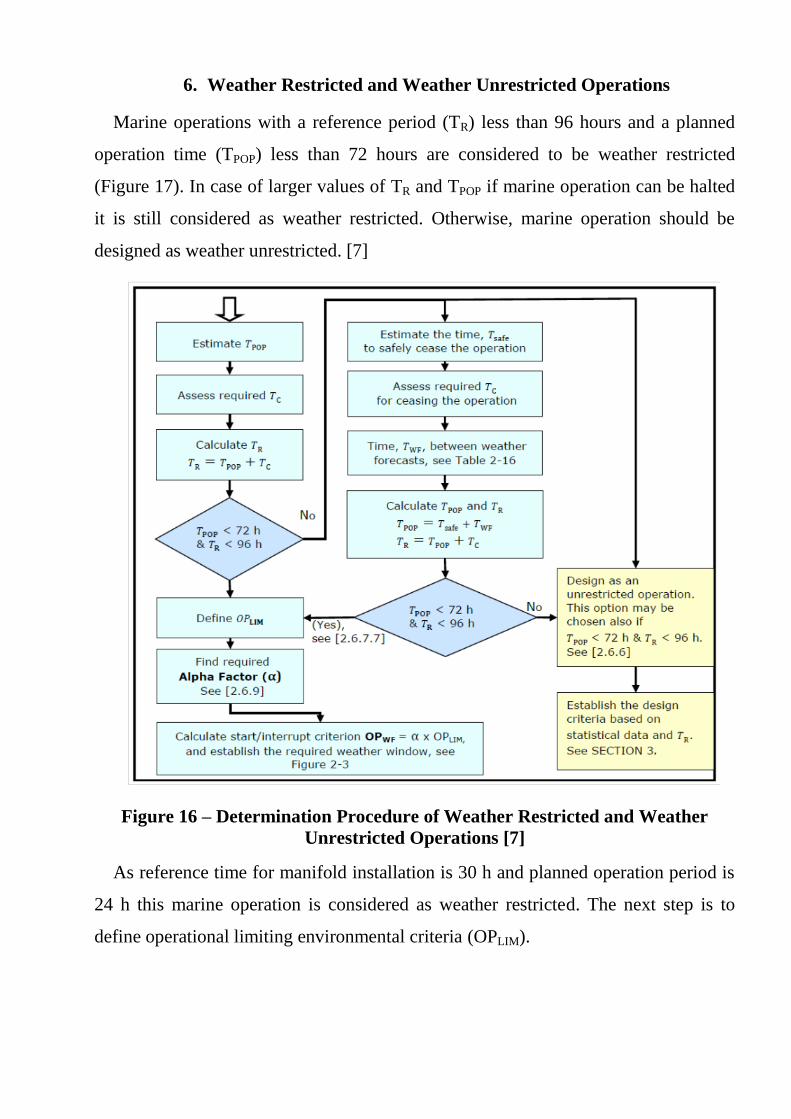
6. Weather Restricted and Weather Unrestricted Operations
Marine operations with a reference period (TR) less than 96 hours and a planned
operation time (TPOP) less than 72 hours are considered to be weather restricted
(Figure 17). In case of larger values of TR and TPOP if marine operation can be halted
it is still considered as weather restricted. Otherwise, marine operation should be
designed as weather unrestricted. [7]
Figure 16 – Determination Procedure of Weather Restricted and Weather
Unrestricted Operations [7]
As reference time for manifold installation is 30 h and planned operation period is
24 h this marine operation is considered as weather restricted. The next step is to
define operational limiting environmental criteria (OPLIM).
7. Operational Limiting Environmental Criteria
Environmental loads for weather restricted operations are selected independent of
statistical data. For weather unrestricted marine operations the design criteria is based
on extreme value statistics.
The OPLIM depend on: [7]
The environmental design criteria.
Maximum wind and waves for safe working or personnel transfer.
Weather restrictions determined for equipment.
Limiting weather conditions of diving system (if any).
Limiting conditions for position keeping systems.
Any limitations identified, e.g. in HAZID/HAZOP, based on operational
experience with involved vessel(s), equipment, etc.
Limiting weather conditions for carrying out identified contingency plans.
DNV GL Standard [7] defines some equipment limitations for subsea lifting
operation. That is why analysis should be performed to not exceed these restrictions.
Than simulations are carried out to define which value of environmental parameters
leads to exceeding equipment limitations. It is easy to check which values of Hs and
Tp correspond to extreme tension, for instance, in slings or crane fall utilizing special
software (e.g. OrcaFlex).
As an example, key points of Kirinskoye manifold lift analysis are introduced
bellow: [4]
1. Acceptance criteria for operations:
o The minimum clearance between the lifting equipment or the crane
boom and any other object/structure should normally not be less than
3m.
o The manifold should not tilt more than 2 degrees in any direction.
o The crane includes a Dynamic Amplification Factor (DAF) of 1.3.
o The slings are designed for a DAF of 2.0.
30
o Utilization Factor (UF) should always be greater than zero.
2. Analyzed environmental conditions:
o Hs = 0.75-2.5 m (changed values).
o Tp = 6-10 s (changed values).
o Pierson-Moskowitz wave spectrum.
o Different angles wave headings.
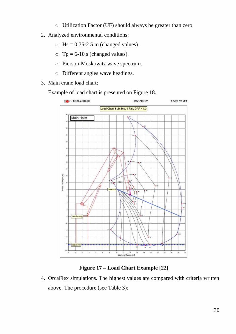
3. Main crane load chart:
Example of load chart is presented on Figure 18.
Figure 17 – Load Chart Example [22]
4. OrcaFlex simulations. The highest values are compared with criteria written
above. The procedure (see Table 3):
31
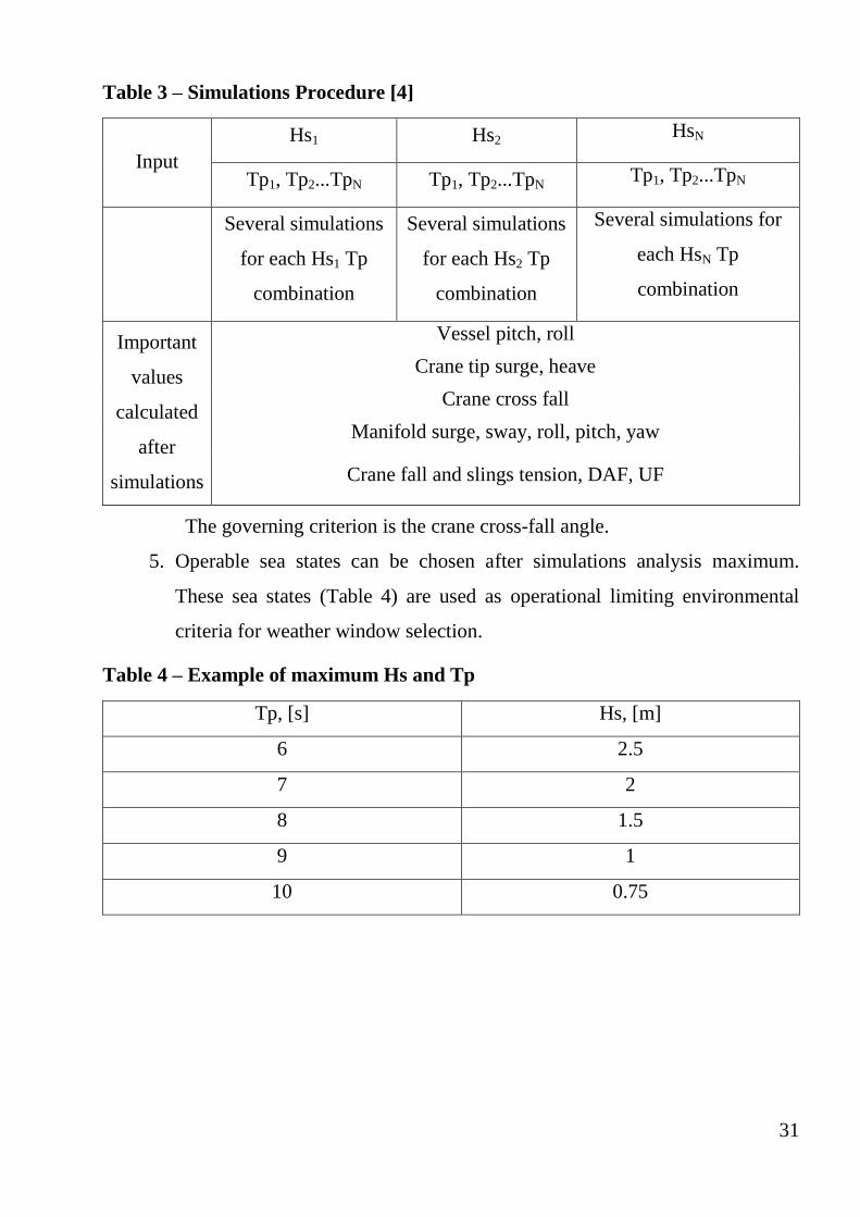
Table 3 – Simulations Procedure [4]
Input
Hs1 Hs2 HsN
Tp1, Tp2...TpN Tp1, Tp2...TpN Tp1, Tp2...TpN
Several simulations
for each Hs1 Tp
combination
Several simulations
for each Hs2 Tp
combination
Several simulations for
each HsN Tp
combination
Important
values
calculated
after
simulations
Vessel pitch, roll
Crane tip surge, heave
Crane cross fall
Manifold surge, sway, roll, pitch, yaw
Crane fall and slings tension, DAF, UF
The governing criterion is the crane cross-fall angle.
5. Operable sea states can be chosen after simulations analysis maximum.
These sea states (Table 4) are used as operational limiting environmental
criteria for weather window selection.
Table 4 – Example of maximum Hs and Tp
Tp, [s] Hs, [m]
6 2.5
7 2
8 1.5
9 1
10 0.75
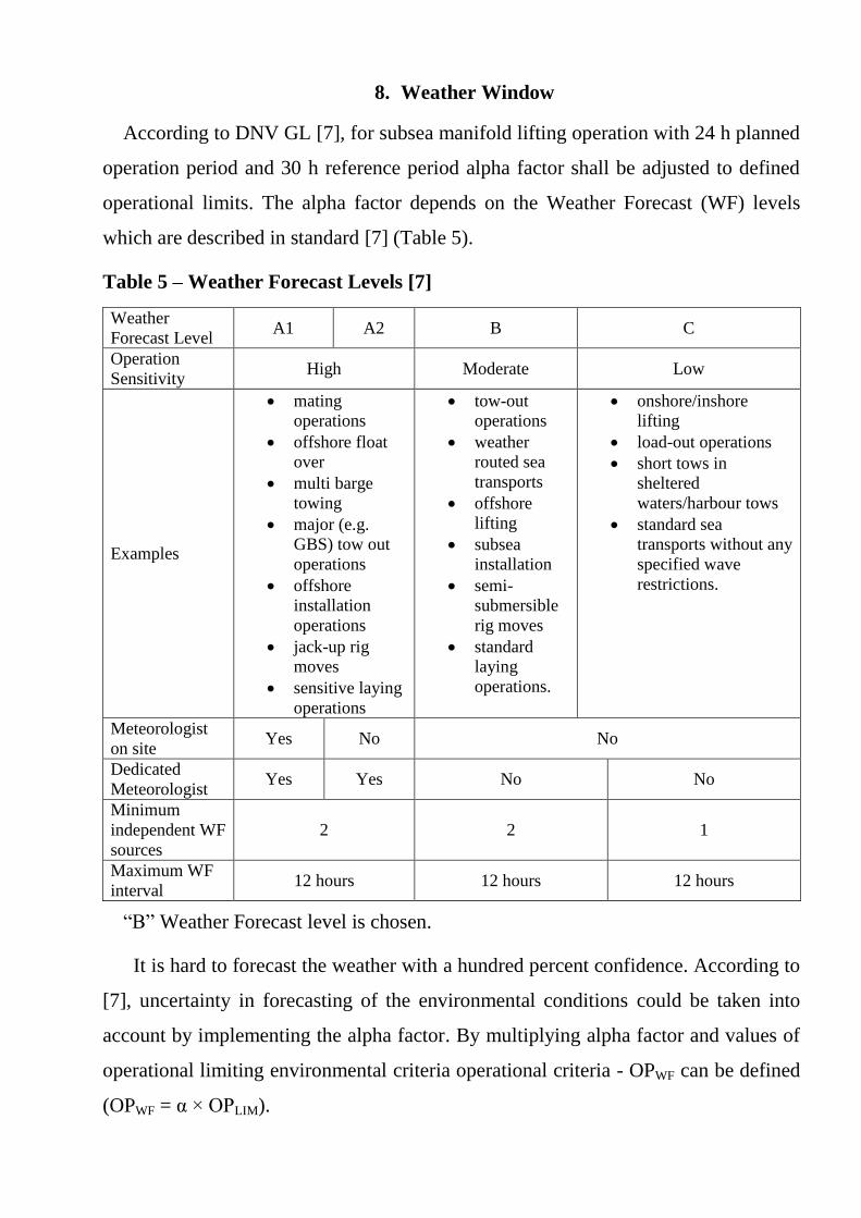
8. Weather Window
According to DNV GL [7], for subsea manifold lifting operation with 24 h planned
operation period and 30 h reference period alpha factor shall be adjusted to defined
operational limits. The alpha factor depends on the Weather Forecast (WF) levels
which are described in standard [7] (Table 5).
Table 5 – Weather Forecast Levels [7]
Weather
Forecast Level A1 A2 B C
Operation
Sensitivity High Moderate Low
Examples
mating
operations
offshore float
over
multi barge
towing
major (e.g.
GBS) tow out
operations
offshore
installation
operations
jack-up rig
moves
sensitive laying
operations
tow-out
operations
weather
routed sea
transports
offshore
lifting
subsea
installation
semi-
submersible
rig moves
standard
laying
operations.
onshore/inshore
lifting
load-out operations
short tows in
sheltered
waters/harbour tows
standard sea
transports without any
specified wave
restrictions.
Meteorologist
on site Yes No No
Dedicated
Meteorologist Yes Yes No No
Minimum
independent WF
sources
2 2 1
Maximum WF
interval 12 hours 12 hours 12 hours
“B” Weather Forecast level is chosen.
It is hard to forecast the weather with a hundred percent confidence. According to
[7], uncertainty in forecasting of the environmental conditions could be taken into
account by implementing the alpha factor. By multiplying alpha factor and values of
operational limiting environmental criteria operational criteria - OPWF can be defined
(OPWF = α × OPLIM).
33
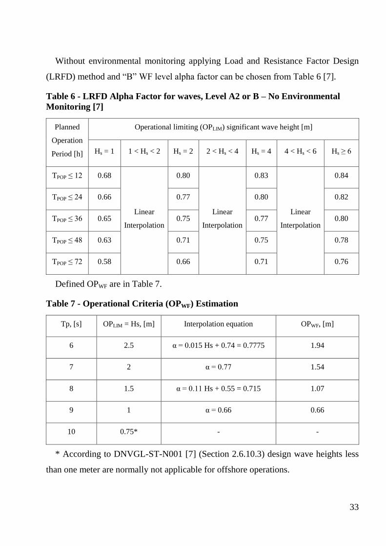
Without environmental monitoring applying Load and Resistance Factor Design
(LRFD) method and “B” WF level alpha factor can be chosen from Table 6 [7].
Table 6 - LRFD Alpha Factor for waves, Level A2 or B – No Environmental
Monitoring [7]
Planned
Operation
Period [h]
Operational limiting (OPLIM) significant wave height [m]
Hs = 1 1 < Hs < 2 Hs = 2 2 < Hs < 4 Hs = 4 4 < Hs < 6 Hs ≥ 6
TPOP ≤ 12 0.68
Linear
Interpolation
0.80
Linear
Interpolation
0.83
Linear
Interpolation
0.84
TPOP ≤ 24 0.66 0.77 0.80 0.82
TPOP ≤ 36 0.65 0.75 0.77 0.80
TPOP ≤ 48 0.63 0.71 0.75 0.78
TPOP ≤ 72 0.58 0.66 0.71 0.76
Defined OPWF are in Table 7.
Table 7 - Operational Criteria (OPWF) Estimation
Tp, [s] OPLIM = Hs, [m] Interpolation equation OPWF, [m]
6 2.5 α = 0.015 Hs + 0.74 = 0.7775 1.94
7 2 α = 0.77 1.54
8 1.5 α = 0.11 Hs + 0.55 = 0.715 1.07
9 1 α = 0.66 0.66
10 0.75* - -
* According to DNVGL-ST-N001 [7] (Section 2.6.10.3) design wave heights less
than one meter are normally not applicable for offshore operations.
34
Note that uncertainty in the forecasted wave periods should also be taken into
account.
Finally, the weather window could be defined.
Required weather window could be estimated by searching a time interval when
the operation will be completed. The operation is considered completed when the
object is in a safe condition. For manifold lifting operation this condition will be the
end of all scope of work.
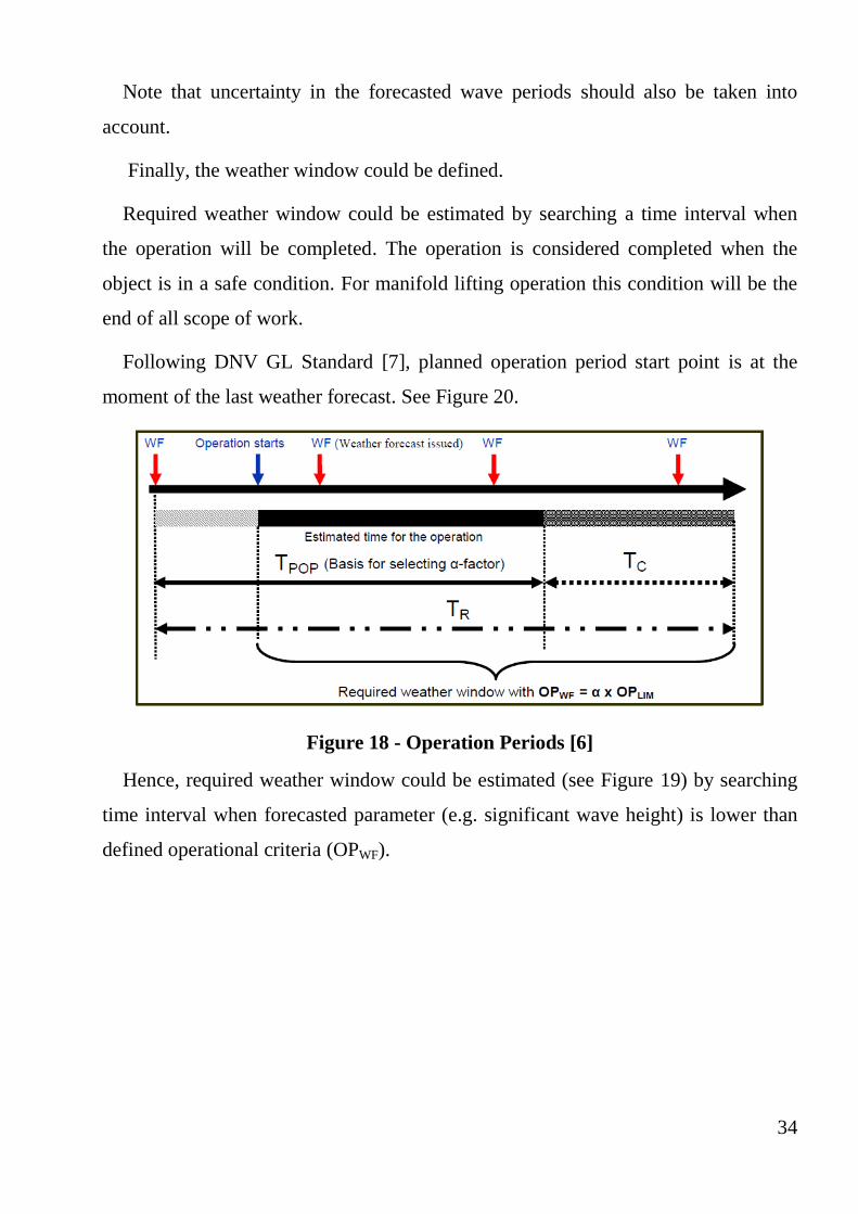
Following DNV GL Standard [7], planned operation period start point is at the
moment of the last weather forecast. See Figure 20.
Figure 18 - Operation Periods [6]
Hence, required weather window could be estimated (see Figure 19) by searching
time interval when forecasted parameter (e.g. significant wave height) is lower than
defined operational criteria (OPWF).
35
Figure 19 – The Weather Window Example for Manifold Lifting Operation
8.1. Weather Forecast
According to [7], the weather forecasts should be received at regular intervals
before and during the manifold installation. Different providers should be the sources
of independent weather forecasts (the most severe weather forecasts is preferred in
case of difference between them). Public weather forecasts are not applicable for
subsea lifting operations.
DNV GL [7] requires that the weather forecast should have general description of
the weather situation and the predicted development and information about:
- wind speed and direction,
- waves and swell, significant and maximum height, mean or peak period and
direction,
- rain, snow, lightning, ice etc.,
- tide variations and/or storm surge,
- visibility,
- temperature, and
- barometric pressure
0
0,5
1
1,5
2
2,5
3
3,5
4
4,5
0 20 40 60 80 100 120 140 160 180
Hs
Hours
OPwf
Forecast
WW

36
- possibility for squalls and polar lows.
The weather forecasts should be issued for each 12 hours for minimum the TR + 24
h. Also an outlook for at least the next 24 hours should be added. Standard [7] defines
the levels of WF according to operational sensitivity to weather conditions and the
operation reference period (see Table 5).

9. Probability of Exceeding the Operational Environmental Limiting
Criteria
According to DNV GL Standard [7], the following should be checked to select
appropriate alpha factor for waves:
“The expected uncertainty in the weather forecast should be calculated based
on statistical data for the actual site and the operation schedule, i.e. TPOP. The
Alpha Factor should be calibrated to ensure that the probability of exceeding
the operational environmental limiting criteria (OPLIM) by more than 50% in
LRFD is less than 10-4
.”
According to long term wave statistics ( [23] , Table 8), the most frequently
appeared wave heights and periods in the Sea of Okhotsk could be defined. Note: H3%
is the wave height with 3% probability of exceedance defined value.
Table 8 – Joint Distribution of H3% and Wave Period for ice-free period [23]
H3%, [m] Wave period, [s]
2-4 4-6 6-8 8-10 10-12
0-2 3.1 35.5 8.9 0.8 0.07
2-4 1.4 22.4 10.6 0.9 0.06
4-6 0.14 5.0 6.3 0.9 0.02
6-8 0.4 1.8. 0.8 0.02
8-10 0.2 0.4 0.03
10-12 0.01 0.11 0.02
Wave period Probability Density Functions (PDF) for H3% 0-2 m and H3% 2-4 m
are shown in Figure 20.
38
Figure 20 – Wave Period PDF for H3% 0-2 m and H3% 2-4 m
Analysing Figure 20, it could be said that waves with 4-6 seconds periods are the
most frequently appeared when wave heights do not exceed 4 m. Larger wave periods
are common for larger wave heights.
According to [22], JONSWAP spectrum at γ = 2 ± 1 for Hs/Tp2 < 0.03 and γ =1.4
± 0.4 for Hs/Tp2 ≥ 0.03 is adopted for the assessment of spectra in the Sea of
Okhotsk. Significant wave height, Hs (100 year return period) = 9.3 m. Wave
spectrum peak period (100 year return period) = 14.6 s.
Figure 21 – JONSWAP Spectrum (based on [22])
0
5
10
15
20
25
30
35
40
PD
F
Wave period, [s]
H3% 0-2 m H3% 2-4 m
0
20
40
60
80
100
120
140
160
0 0,1 0,2 0,3 0,4
Sp
ectr
al d
ensi
ty,
m2s
Frequency, Hz
SΞΞ(f)
hs=9.3 m, tp=14.6 s
39
However, for the purpose of designing marine operations simulations should be
performed for the sea states assumed to be the limiting sea states for the operations
[23]. For Kirinskoye field lifting analysis Pierson-Moskowitz wave spectrum was
chosen. [23]: “If extreme loads are established, it is important to repeat the
simulations with different random seed in order to reflect in inherent randomness of
loads/responses that can be experienced during the operation. The number of
simulations depends on the selected probability level for the characteristic design
loads. This means that the design process must be established before the program for
the simulations can be determined. A good rule of thumb is that one should select the
number of repetitions so high that one can expect to see some few realizations above
this level.”
For the first pair of Hs and Tp values (see Table 4) the wave height with 10-4
probability of exceedance is defined. After that, for fixed Tp another Hs value is
estimated such that the 50% increased value of this wave height will correspond to
10-4
probability of exceedance. Estimated Hs value is compared with OPLIM and,
finally, alpha factor could be defined.
Acceptable exceedance for whole operation is 𝐹ℎ𝑠(ℎ𝑠,24ℎ) =10-4
. In order to be
successful during operation we must be successful for all 3 hour periods in 24 hour
TPOP:
1 − 𝐹ℎ𝑠(ℎ𝑠,24ℎ) = (1 − 𝐹ℎ𝑠(ℎ𝑠,3ℎ))
243
𝑃 = 𝐹ℎ𝑠(ℎ𝑠,3ℎ) = 1 − (1 − 𝐹ℎ𝑠(ℎ𝑠,24ℎ))
18
For Gaussian surface elevation process distribution of global maxima (global crest
height) is Rayleigh distribution [19]:
CDF: 𝐹𝑐𝐺(𝑐) = 1 − 𝑒(−
1
2(𝑐
𝜎𝛯)2
)
Distribution of 3 hours maximum crest height:
40
𝑃 = 𝐹𝑐3ℎ(𝑐) = (1 − 𝑒(−
12(𝑐𝜎𝛯
)2))
𝑛3ℎ
The zero-up-crossing wave period 𝑡02 may be related to the peak period by the
following approximate relations (1 ≤ 𝛾 ≤ 7) [23] (note: 𝛾 = 𝑐𝑜𝑛𝑠𝑡 = 1 for PM wave
spectrum):
𝑡02𝑇𝑝
= 0.6673 + 0.05037𝛾 − 0.006230𝛾2 + 0.0003341𝛾3
Number of waves in 3 hour: 𝑛3ℎ =𝑇
𝑡02=
3×3600
0.726×𝑇𝑝
Assume that variance is equal to [23]: 𝜎𝛯2 =
1
16𝐻𝑠2
As a result of calculations (see Appendix A) new Hs value is estimated such that
the 50% increased value of OPLIM wave height corresponds to 10-4
probability of
exceedance.
Figure 22 – Cumulative Distribution Functions Calculated for Different Hs
Calibrated alpha factor is 0.641. In case of 56% higher value of forecasted Hs than
OPLIM value, the probability of exceeding the operational environmental limiting
criteria (OPLIM) by more than 50% in LRFD is less than 10-4
.
0,0000001
0,000001
0,00001
0,0001
0,001
0,01
0,1
1
0 1 2 3 4 5 6 7 8 9
CD
F
c, m
1-Fc3h(c)
OPlim New Hs
10. Icing
Strong wind, big wave height and low air temperature are common conditions for
the Sea of Okhotsk which could be observed since autumn. Such conditions are
contributes to vessel icing. This phenomenon should be taken into account as big
amount of ice causes some problems to perform marine operation such as slippery
deck, blocked exits and equipment as well as vessel instability. Icing is very
dangerous for fishing boat. There are some examples when fishing boats are capsized
because of severe icing on the deck which was the reason of vessel reduced stability.
As for big vessels with high free board, icing could lead to safety level decreasing.
However, if possible icing conditions are forecasted and icing rate is defined, marine
operation can be planned with special precautions to perform risk reduction activities.
Icing phenomenon has been studied for a long period. Some icing prediction
models was introduced, however, today researchers are still trying to improve their
models to make more accurate predictions.
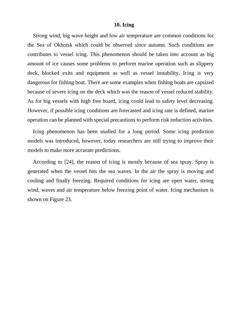
According to [24], the reason of icing is mostly because of sea spray. Spray is
generated when the vessel hits the sea waves. In the air the spray is moving and
cooling and finally freezing. Required conditions for icing are open water, strong
wind, waves and air temperature below freezing point of water. Icing mechanism is
shown on Figure 23.
42
Figure 23 – Wet Icing. Heat Fluxes (continuous spray) [24]
The terms in Figure 23 are defined as follows:
𝑄𝑟 – radiation. This term could be neglected due to no sun during storm.
𝑄𝑑 = 𝑅𝑐𝑤(𝑇𝑓 − 𝑇𝑑) – spray cooling due to freezing temperature.
R – spray flux during spraying, 𝑐𝑤 – specific heat capacity of water, 𝑇𝑑 – droplet
temperature, 𝑇𝑓 = −𝑆𝑏
0.0182 – freezing temperature which depends on water salinity.
𝑄𝑐 = ℎ(𝑇𝑓 − 𝑇𝑎) – convective heat flux.
𝑇𝑎 – air temperature, ℎ - heat transfer coefficient.
ℎ =𝑁𝑢𝑘𝑎
𝐿, 𝑁𝑢 = 0.03𝑅𝑒0.8 – for turbulent flow, 𝑅𝑒 =
𝑉𝐿
𝜈, 𝑘𝑎 – thermal
conductivity of air, 𝐿 – characteristic size.
𝑄𝑒 = 0.017ℎ (𝑒𝑣(𝑇𝑓) − 𝑟𝐻𝑒𝑣(𝑇𝑎)) – evaporative heat flux.
𝑒𝑣(𝑇) = 611.2𝑒17.67𝑇
𝑇+243.5 – saturated vapour pressure for given temperature, 𝑟𝐻 –
relative humidity of air.
𝑄𝑘 = 𝑘𝑖𝑐𝑒𝑑𝑇
𝑑𝑏 – conduction heat flux (this term is neglected in calculations).
43
𝑘𝑖𝑐𝑒 – heat conductivity of ice, 𝑏 – ice thickness.
For periodic spray the heat equation becomes:
𝑙𝑓(1 − 𝑘∗)𝐼 = 𝑄𝑐 + 𝑄𝑒 +𝑡𝑑𝑢𝑟
𝑡𝑝𝑒𝑟𝑄𝑑
𝑙𝑓 – latent heat of fusion of water, 𝐼 – ice accretion rate, 𝑘∗ ≈ 0.3 – the interfacial
distribution coefficient.
Assume the freezing temperature (due to different salinity content) and droplets
temperature to be random variables with normal distributions. Monte Carlo
simulations (see Appendix B) will be used to estimate the probability distribution
function of ice growth.
Samuelsen E. [25] collected icing-rate severity categories from different literature
sources in one table (see Table 9). Upper boundary icing-rate value of light icing in
Overland classification is considered in this report. Minimum ice on the deck gives
the smallest safety risk.
Table 9 – Icing-rate Severity Categories [25]
Category/Source Mertins (1968) LUa
WMOb
WCc
BRd
Overlande
Trace - - - 0.25-0.64 cm
(3 h)-1
<0.20 cm
h-1 -
Light 1-3 cm (24 h)-1 0.5-2 cm (12
h)-1
1 cm (3 h)
-1
0.64-1.27 cm
(3 h)-1
0.20-0.40
cm h-1
<0.70 cm
h-1
Moderate 4-6 cm (24 h)-1
1-3 cm (4 h)-1
1-5 cm (3 h)-1
1.27-1.91 cm
(3 h)-1
0.40-0.96
cm h-1
0.7-2.0 cm
h-1
Severe 7-14 cm (24 h)-1
>4 cm (4 h)-1
6-12 cm (3 h)-1
1.91-3.18 cm
(3 h)-1
>0.96 cm
h-1
2.0-4.0 cm
h-1
Very severe ≥15 cm (24 h)-1
- >12 cm (3 h)-1
>3.18 cm (3
h)-1
- >4.0 cm h
-1
Icing-rate unit (cm h-1
)
Light ≤0.17 ≤0.25 ≤0.33 ≤0.42 ≤0.40 ≤0.70
Moderate 0.17-0.29 0.25-1.0 0.33-2.0 0.42-0.64 0.40-0.96 0.7-2.0
Severe >0.29 >1.0 >2.0 >0.64 >0.96 >2.0 a Lundqvist and Udin (1977).
b WMO definition from 1975 according to Lundqvist and Udin (1977).
c Wise and Comiskey (1980). d Brown and Roebber (1985)
e Overland et al. (1986) and very severe from Overland (1990).

44
For certain weather conditions the probability of exceedance 7 mm/hr ice growth
value will be estimated.
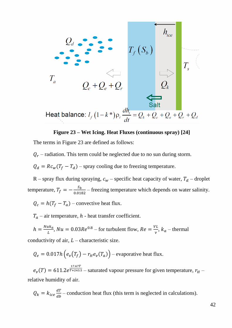
11. Ice Growth Calculation
Ice growth distribution is shown on Figure 24. Matlab code is in Appendix C.
Figure 24 – Ice Growth Probability Density Function
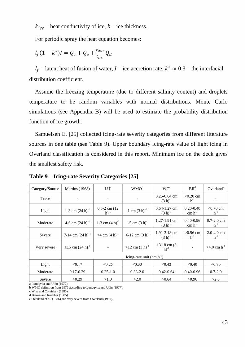
A cumulative probability distribution is defined (see Figure 25) to calculate
probability of exceeding the required value of ice growth.
Figure 25 - CDF of Ice Growth
Probability of exceeding 7 mm/hr ice growth is 𝐸𝐷𝐹 = 1 − 𝐶𝐷𝐹 = 0.034 (see
Figure 26).
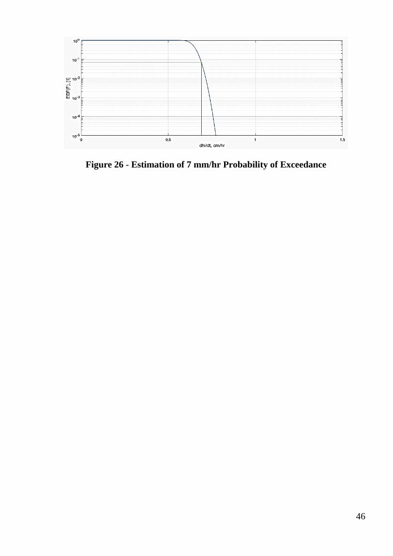
46
Figure 26 - Estimation of 7 mm/hr Probability of Exceedance

12. Discussions
12.1. Weather Window Estimation
A huge scope of work should be performed before subsea manifold installation.
The manifold lift analysis should be carried out to satisfy safety requirements. The
basic theory in such analysis is the stochastic approach of sea state description. When
operational limiting criteria are established the weather window can be defined.
Following LRFD approach, the probability of exceedance the operational limiting
criteria by more than 50% should be less than 10-4
. According to this, calibrated alpha
factor was defined.
12.2. Calculated Probability of Exceedance icing-rate value
Performed calculations give only rough estimation of exceedance probability.
More accurate models are based on high quality data and specific vessel parameters.
Moreover, computational fluid dynamics principals are applied in these models. More
information about ship-icing prediction methods is available in [25].
However, general icing physics was applied with utilizing of two parameters as
random variables with normal probability density functions. Monte Carlo simulation
with three hundred iterations was used to define icing-rate PDF. Hence, CDF was
defined to estimate the probability of exceedance 7 mm/h icing-rate. If in LRFD 10-4
probability of exceedance limiting value is established, the chosen weather conditions
are not suitable for marine operation performing.
13. Conclusion
The procedure of weather window estimation which is based on DNVGL-ST-N001
Standard [7] was shown in this report. As the sea state could not be described by
deterministic values of several parameters, limiting factors of marine operations are
estimated by a probabilistic approach. It is important to operate in such conditions
that probability of exceedance of limiting value will be very low.
The DNV GL Standard [7] procedure (for the wave limiting factor) was applied for
Sea of Okhotsk conditions. It was shown how to describe the sea state. The weather
window for a specific vessel and possible marine operation was estimated. And
finally, the probability of exceedance the limiting values was calculated.
Due to short ice-free period in the Sea of Okhotsk companies will have less time to
perform marine operations. Ship icing has to be analyzed to stay safe while working
in autumn period. The basic analysis procedure is shown in this report.
References
[1] “PJSC Gazprom,” [Online]. Available:
http://www.gazprom.com/f/posts/62/971877/infographics-kirinskoye-en.jpg.
[Accessed 4 April 2018].
[2] E. V. Petrenko, “Subsea Technology - The Key Solution for The Arctic and Far
East fields development,” in 13th International Conference and Exhibition for
Oil and Gas Resources Development of the Russian Arctic and CIS Continental
Shelf, Saint-Petersburg, 2017.
[3] “PJSC Gazprom,” [Online]. Available:
http://www.gazprom.com/f/posts/19/374463/sakhalin3-map-01-en-2016-04.png.
[Accessed 15 January 2018].
[4] S. Nesterenko, Information regarding manifold installation during Kirinskoye
field development, 2018.
[5] DNV GL, Lifting Operations (VMO Standard - Part 2 - 5), DNV-OS-H205,
2014.
[6] DNV GL, Marine Operations, General, DNV-OS-H101, 2011.
[7] DNV GL, Marine operations and marine warranty, DNVGL-ST-N001, 2016.
[8] A. I. Ermakov and V. S. Vovk, “Meteorological and Hydrogeological Conditions
of the North Eastern Coast of Sakhalin Island in the Okhotsk Sea,” in Basics of
Offshore Petroleum Engineering and Development of Marine Facilities,
Stavanger, Moscow, St Petersburg, Trondheim, Oil and Gas, 1999, pp. 137-143.
[9] “Exxon Neftegas Limited,” [Online]. Available: http://www.sakhalin-1.com/en-
ru/company/about-us/phases-and-facilities. [Accessed 5 April 2018].
50
[10] “ITOCHU Group,” [Online]. Available:
http://www.itochuoil.co.jp/e/project/001_sakhalin.html. [Accessed 15 April
2018].
[11] “PJSC Gazprom,” [Online]. Available:
http://www.gazprom.com/about/production/projects/lng/sakhalin2/. [Accessed
15 April 2018].
[12] M. N. Mansurov and E. V. Zakharov, “Sakhalin 3: The Geological and
Engineering Principles,” ROGTEC, no. 30, pp. 48-57.
[13] Sapozhnikov et al., “Hydrochemical Atlas of the Sea of Okhotsk 2001,”
[Online]. Available: https://www.nodc.noaa.gov/OC5/okhotsk/ok_doc.html#1..
[Accessed 12 January 2018].
[14] “ESIMO,” [Online]. Available:
http://portal.esimo.ru/dataview/viewresource?resourceId=RU_RIHMI-
WDC_929¶meter=tempair&sea=okhot. [Accessed 20 April 2018].
[15] S. Duplensky, Information regarding typical time needed for Marine
Operations, Stavanger, 2017.
[16] D. A. Mirzoev, Information regarding Yuzhno-Kirinskoye field development,
Moscow, 2018.
[17] V. A. Golubev, “Gazprom activities on Russian Shelf,” in International
Conference and Exhibition for Oil and Gas Resources Development of the
Russian Arctic and CIS Continental Shelf, Saint Petersburg, 2013.
[18] “SolstadFarstad ASA,” [Online]. Available: https://solstad.no/wp-
content/uploads/2014/01/Oceanic_ok_Part1.pdf. [Accessed 10 November 2017].
51
[19] S. Haver, “Lecture notes. OFF600 Marine Operations course,” Stavanger, 2017.
[20] “offshore-crane.com,” [Online]. Available: https://www.offshore-
crane.com/120-ton-nov-subsea-knuckleboom-crane-for-sale/. [Accessed 20 May
2018].
[21] Russian Maritime Register of Shipping (RS), “Wind and Waves Statistical Data
in Barents Sea, Sea of Okhotsk and Caspian Sea,” Saint Petersburg, 2003.
[22] G. V. Zhukov and S. V. Karlinsky, “Production Platforms for Russian Offshore,”
in The Sixth ISOPE Pacific/Asia Offshore Mechanics Symposium, 2004.
[23] S. Haver, “Metocean Modelling and Prediction of Extremes,” Stavanger, 2017.
[24] DNV GL, Environmental conditions and environmental loads, DNV-RP-C205.,
2010.
[25] A. Kulyakhtin, Icing, the course AT-327, UNIS, 2017.
[26] E. M. Samuelsen, “Ship-icing Prediction Methods Applied in Operational
Weather Forecasting,” Quarterly Journal of the Royal Meteorological Society,
no. Volume 144, issue 710, 2017.
[27] A. Shestov, Ice actions - Probabilistic approach (Monte Carlo Simulation), the
course AT-327, UNIS, 2017.
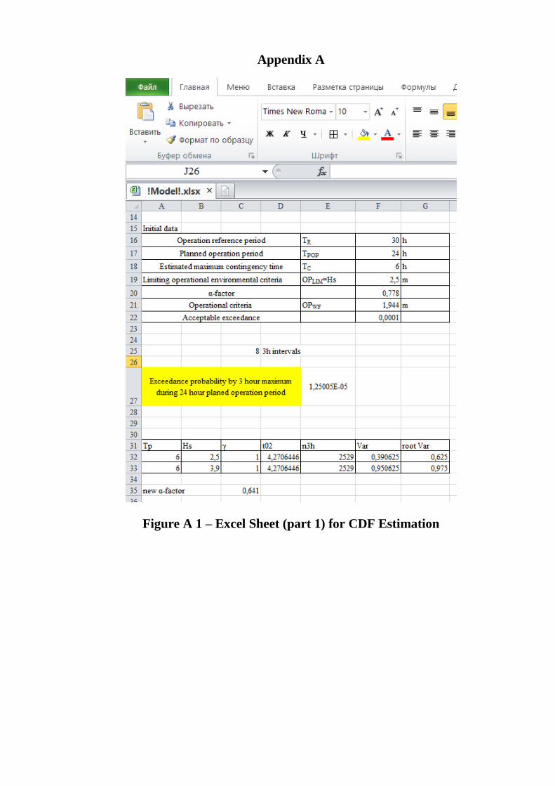
Appendix A
Figure A 1 – Excel Sheet (part 1) for CDF Estimation

53
Figure A 2 - Excel Sheet (part 2) for CDF Estimation
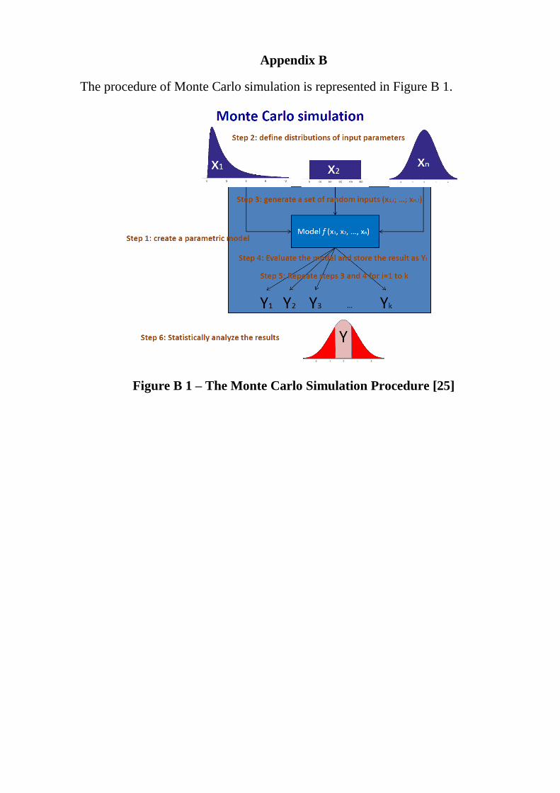
Appendix B
The procedure of Monte Carlo simulation is represented in Figure B 1.
Figure B 1 – The Monte Carlo Simulation Procedure [25]
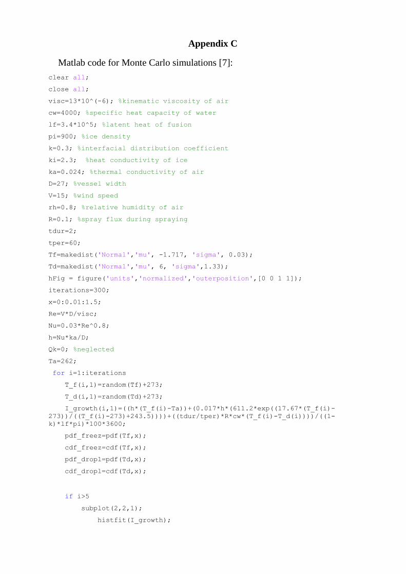
Appendix C
Matlab code for Monte Carlo simulations [7]:
clear all;
close all;
visc=13*10^(-6); %kinematic viscosity of air
cw=4000; %specific heat capacity of water
lf=3.4*10^5; %latent heat of fusion
pi=900; %ice density
k=0.3; %interfacial distribution coefficient
ki=2.3; %heat conductivity of ice
ka=0.024; %thermal conductivity of air
D=27; %vessel width
V=15; %wind speed
rh=0.8; %relative humidity of air
R=0.1; %spray flux during spraying
tdur=2;
tper=60;
Tf=makedist('Normal','mu', -1.717, 'sigma', 0.03);
Td=makedist('Normal','mu', 6, 'sigma',1.33);
hFig = figure('units','normalized','outerposition',[0 0 1 1]);
iterations=300;
x=0:0.01:1.5;
Re=V*D/visc;
Nu=0.03*Re^0.8;
h=Nu*ka/D;
Qk=0; %neglected
Ta=262;
for i=1:iterations
T_f(i,1)=random(Tf)+273;
T_d(i,1)=random(Td)+273;
I_growth(i,1)=((h*(T_f(i)-Ta))+(0.017*h*(611.2*exp((17.67*(T_f(i)-
273))/((T_f(i)-273)+243.5))))+((tdur/tper)*R*cw*(T_f(i)-T_d(i))))/((1-
k)*lf*pi)*100*3600;
pdf_freez=pdf(Tf,x);
cdf_freez=cdf(Tf,x);
pdf_dropl=pdf(Td,x);
cdf_dropl=cdf(Td,x);
if i>5
subplot(2,2,1);
histfit(I_growth);
56
xlabel('dhi/dt, cm/hr');
ylabel('number of appearance, [1]');
axis([0 1.5 0 inf]);
subplot(2,2,2);
f=0:0.01:1.5;
pd_I=fitdist(I_growth,'Normal');
pdf_I=pdf(pd_I,f);
cdf_I=cdf(pd_I,f);
plot(i,pd_I.sigma/pd_I.mu*100,'.r'); hold on;
grid on;
axis([0 iterations 0 inf] )
xlabel('iteration number');
ylabel('\sigma / \mu, %');
subplot(2,2,3);
plot(f, cdf_I);
xlabel('dhi/dt, cm/hr');
ylabel('CDF(dhi/dt), [1]');
grid on;
subplot(2,2,4);
if i>6
set(h1,'Visible','off');
set(h2,'Visible','off');
set(h3,'Visible','off');
end
edf_I=1-cdf_I;
h1=plot(f, edf_I);hold on;
set(gca, 'YScale', 'log');
axis([0 1.5 10^-5 1]);
xlabel('dhi/dt, cm/hr');
ylabel('EDF(F), [1]');
grid on;
SL=max(find(f<0.7));
a=SL;
h2=stem(f(a),edf_I(a),'.g');
xx=[0 f(a)]; yy=[edf_I(a) edf_I(a)];
h3=plot(xx,yy,'g');

57
pause(0.001);
end
end