Failure Evasion: Statistically Solving the NP Complete

Failure Evasion: Statistically Solving the NP Complete Problem of TestingDifficult-to-Detect Faults

by

Muralidharan Venkatasubramanian

A dissertation submitted to the Graduate Faculty ofAuburn University

in partial fulfillment of therequirements for the Degree of

Doctor of Philosophy

Auburn, AlabamaDecember 10, 2016

Keywords: Database search, digital test, quantum computing, test generation, probabilisticcorrelation, Mahalanobis distance

Copyright 2016 by Muralidharan Venkatasubramanian

Approved by

Vishwani D. Agrawal, Chair, James J. Danaher Professor of Electrical and ComputerEngineering

Adit D. Singh, James B. Davis Professor of Electrical and Computer EngineeringVictor P. Nelson, Professor of Electrical and Computer Engineering

Michael C. Hamilton, Associate Professor of Electrical and Computer EngineeringRoy J. Hartfield, Professor of Aerospace Engineering

Abstract

A circuit with n primary inputs (PIs) has N = 2n possible input vectors. A test

vector to correctly detect a fault in that circuit must be among those 2n n-bit combinations.

Clearly, this problem can be rephrased as a database search problem. It is colloquially

known that using a pure random test generator to test for faults in a digital circuit is

horribly inefficient. To overcome this inefficiency, various testing algorithms were successfully

developed and implemented over the last 50 years. Classic algorithms like the D-algorithm,

PODEM and FAN have long been foundations other algorithms have built upon to vastly

improve the search time for test vectors.

Because searching for the last few faults that are hard to detect is mathematically

NP complete, it can become computationally expensive to attain 100% fault coverage in a

finite amount of time. Contemporary algorithms usually generate new test vectors based on

properties of previous successful ones and hence enter a bottleneck when trying to find tests

for these hard to detect stuck-at faults, as their test properties may not match previous test

successes.

Since, all testing algorithms can be interpreted as unsorted database search methods, it

is to our benefit if we choose to create a testing algorithm based on an efficient solution to

database search. Currently, it has been shown that Grover’s quantum computing algorithm

is the best solution to search a database of N elements with sub-linear O(√N ) complexity,

while most other algorithms are linear or O(N). Hence, it is clear that creating a testing

algorithm that emulates Grover’s algorithm for finding test vectors could be a faster solution

for VLSI testing.

We hypothesize that avoiding the properties of failed vectors by learning from each fail-

ure would lead to a solution in fewer iterations. We use a statistical method to maximize the

ii

“Mahalanobis distance” from the failed vectors while simultaneously reducing the distance

to “activation/propagation vectors”. Our results show that this technique is very efficient in

finding tests for these final hard to detect stuck-at faults.

For the b12 combinational benchmark circuit with 15 primary inputs (PIs), a random

search, on average, took 16,367 iterations to find a test for a difficult to detect stuck-at

fault. Our best algorithm was able to find a test, on average, in 311 iterations for the same

fault. While it is not the best result when compared to a quantum search (which needs 181

iterations on average), it is still about two orders of magnitude better when compared to a

random search and hence is significant. This work presents the idea and a detailed analysis

of how our algorithm functions and results for several benchmark circuits.

iii

Acknowledgments

First of all, I would like to thank the Electrical and Computer Engineering (ECE)

department for supporting my graduate study by providing me a Teaching Assistantship

(TA) without which I would not have been able to complete my PhD work successfully. I

would also like to thank Dr. Prathima Agrawal for giving me a Research Assistantship (RA)

in my first semester and for providing me moral support and constructive criticism which

have been immensely helpful.

I am extremely grateful to have Dr. Vishwani Agrawal as my advisor and mentor.

His vast knowledge of the subject, tremendous intuition and constant encouragement and

motivation even during the bleakest of times has been the primary reason in enabling me

to complete my work. His approachability and interests in debating allowed me to bounce

ideas off him and I have learned a lot from our continuous brainstorming sessions.

During the early days of this investigation, Dr. Agrawal visited Dr. Lov Grover in New

Jersey, whom he had known from his days at Bell Labs. Besides agreeing with our analogy

between test search and database search, Dr. Grover appreciated our use of fault simulator

for identifying properties that make some vectors closer to being a test. He, however, made

an observation that a real implementation of an equivalent of his concept of Oracle may

require a quantum computer built at a larger scale than possible today. I am thankful to

Dr. Grover for his encouragement.

I would also like to thank Dr. Adit Singh, Dr. Victor Nelson and Dr. Michael Hamilton

for being part of my dissertation committee. The courses offered by these esteemed professors

broadened my ECE knowledge which in turn stimulated my critical thinking and analysis

skills thereby allowing me to apply these skills to this work. I would also like to thank Dr.

iv

Roy Hartfield for agreeing to be my outside reader and for supporting me as an employee of

his start-up after my masters.

Finally, I would like to thank all my friends and family who have supported me over the

years and have provided me constant encouragement and moral support. Most important of

all, I would like to thank my partner, Keerti, for her never ending support, extreme patience

and endurance while I finished my dissertation. Without her support, I would not have been

able to finish this work successfully.

v

Table of Contents

Abstract . . . . . . . . . . . . . . . . . . . . . . . . . . . . . . . . . . . . . . . . . . . ii

Acknowledgments . . . . . . . . . . . . . . . . . . . . . . . . . . . . . . . . . . . . . . iv

List of Figures . . . . . . . . . . . . . . . . . . . . . . . . . . . . . . . . . . . . . . . viii

List of Tables . . . . . . . . . . . . . . . . . . . . . . . . . . . . . . . . . . . . . . . . xii

List of Abbreviations . . . . . . . . . . . . . . . . . . . . . . . . . . . . . . . . . . . . xiii

1 Introduction . . . . . . . . . . . . . . . . . . . . . . . . . . . . . . . . . . . . . . 1

2 Background . . . . . . . . . . . . . . . . . . . . . . . . . . . . . . . . . . . . . . 4

2.1 Automatic Test Pattern Generation (ATPG) . . . . . . . . . . . . . . . . . . 4

2.1.1 D-Algorithm . . . . . . . . . . . . . . . . . . . . . . . . . . . . . . . . 5

2.1.2 Path-Oriented Decision Making (PODEM) . . . . . . . . . . . . . . . 5

2.1.3 Fanout-Oriented Test Generation (FAN) . . . . . . . . . . . . . . . . 7

2.2 Database Search Algorithms . . . . . . . . . . . . . . . . . . . . . . . . . . . 13

2.3 Interdisciplinary Connection . . . . . . . . . . . . . . . . . . . . . . . . . . . 14

2.4 Quantum Computing - The Future! . . . . . . . . . . . . . . . . . . . . . . . 15

2.5 Grover’s Algorithm - A Possible Solution . . . . . . . . . . . . . . . . . . . . 17

2.6 Application of Grover’s Algorithm in ATPG . . . . . . . . . . . . . . . . . . 19

2.7 Overview of Mahalanobis Distance . . . . . . . . . . . . . . . . . . . . . . . 20

2.8 Applications of Mahalanobis Distance . . . . . . . . . . . . . . . . . . . . . . 22

3 Algorithm Design . . . . . . . . . . . . . . . . . . . . . . . . . . . . . . . . . . . 24

3.1 Version 1 . . . . . . . . . . . . . . . . . . . . . . . . . . . . . . . . . . . . . . 25

3.1.1 Algorithm Steps . . . . . . . . . . . . . . . . . . . . . . . . . . . . . . 26

3.1.2 Algorithm Working Example . . . . . . . . . . . . . . . . . . . . . . . 27

3.2 Version 2 . . . . . . . . . . . . . . . . . . . . . . . . . . . . . . . . . . . . . . 35

vi

3.2.1 Implementation . . . . . . . . . . . . . . . . . . . . . . . . . . . . . . 37

3.3 Version 3 . . . . . . . . . . . . . . . . . . . . . . . . . . . . . . . . . . . . . . 39

3.3.1 Algorithm Steps . . . . . . . . . . . . . . . . . . . . . . . . . . . . . . 40

3.3.2 Test Vector Generation Example . . . . . . . . . . . . . . . . . . . . 41

4 Simulation Setup and Tools . . . . . . . . . . . . . . . . . . . . . . . . . . . . . 47

5 Results and Discussion . . . . . . . . . . . . . . . . . . . . . . . . . . . . . . . . 49

5.1 Version 1 Algorithm Results . . . . . . . . . . . . . . . . . . . . . . . . . . . 49



6 Conclusion . . . . . . . . . . . . . . . . . . . . . . . . . . . . . . . . . . . . . . . 64

vii

List of Figures

2.1 PODEM high-level flowchart [14, 31] . . . . . . . . . . . . . . . . . . . . . . . . 6

2.2 Seven stages of developing of a practical quantum computer [23]. . . . . . . . . 16

2.3 Graph comparing exhaustive search and quantum search highlighting the fact

that exhaustive search taking N/2 iterations while quantum search takes√N

iterations [77]. . . . . . . . . . . . . . . . . . . . . . . . . . . . . . . . . . . . . 20

2.4 Comparison of fault coverage vs. CPU time for exhaustive search (ES), genetic al-

gorithm (GA), DNA based algorithm (DATPG) and quantum search (QATPG) [77]. 21

2.5 Mahalanobis distance calculated for each X and Y variable and shaded according

to distance [39]. . . . . . . . . . . . . . . . . . . . . . . . . . . . . . . . . . . . . 22

3.1 Gate level circuit of the c17 benchmark. ’X’ marks the stuck-at-1 fault site for

which the test vector was to be found. . . . . . . . . . . . . . . . . . . . . . . . 27

3.2 Random: Probability of 32 vectors of c17 for successive iterations (trial vector

generation) during a typical random search for test for stuck-at-1 fault shown in

Fig. 3.1. . . . . . . . . . . . . . . . . . . . . . . . . . . . . . . . . . . . . . . . . 33

3.3 Version 1: Probability of 32 vectors of c17 for successive iterations (trial vector

generation) during a typical Version 1 search for test for stuck-at-1 fault shown

in Fig. 3.1. . . . . . . . . . . . . . . . . . . . . . . . . . . . . . . . . . . . . . . 34

3.4 All test vectors in the vector space classified in appropriate categories for a given

stuck-at fault. . . . . . . . . . . . . . . . . . . . . . . . . . . . . . . . . . . . . . 36

viii

3.5 Flowchart of the implementation of skewing the search in the vector space using

weighted probabilities. . . . . . . . . . . . . . . . . . . . . . . . . . . . . . . . . 38

3.6 A six-input circuit with a target stuck-at-a fault marked as ’X’. . . . . . . . . . 41

5.1 Distribution of the number of iterations needed to find a test for a single stuck-

at-1 fault on an input of a 10-input AND gate using the proposed Version 1

algorithm. Average iterative search duration based on 100 cases is 10 iterations. 50

5.2 Distribution of the number of iterations needed to find a test for a single stuck-

at-1 fault on an input of a 10-input AND gate using the weighted random test

generator [3]. Average iterative search duration based on 100 test generation

cases is 25 iterations. . . . . . . . . . . . . . . . . . . . . . . . . . . . . . . . . . 50

5.3 Distribution of the number of iterations used to find a test for a single stuck-at-1

fault on an input of a 10-input AND gate using a random test generator. Average

iterative search duration based on 100 cases is 512 iterations. . . . . . . . . . . 51

5.4 The c17 benchmark circuit showing two stuck-at-1 faults with minimum number

of tests. . . . . . . . . . . . . . . . . . . . . . . . . . . . . . . . . . . . . . . . . 51

5.5 A six-input circuit with a stuck-at-1 fault for which the test vector is to be found. 52

5.6 One hundred cases of iterative search for a test vector for a fault in the circuit

of Fig. 5.5. Grey bars indicate percentage of times certain number of iterations

were required. The light orange bars indicate similar percentage for the proposed

algorithm (Version 2) [85]. The green bar indicates the theoretical mean = 8 of

Grover’s quantum search. . . . . . . . . . . . . . . . . . . . . . . . . . . . . . . 54

ix

5.7 One hundred cases of iterative search for a test vector for a fault in ALU control

benchmark circuit. Grey bars indicate percentage of times certain number of

iterations were required. The light orange bars indicate similar percentage for

the proposed algorithm (Version 2) [85]. The green bar indicates the theoretical

mean = 11 of Grover’s quantum search. . . . . . . . . . . . . . . . . . . . . . . 55

5.8 One hundred cases of iterative search for a test vector for a fault in decoder





5.9 One hundred cases of iterative search for a test vector for a fault in ones counter





5.10 One hundred cases of iterative search for a test vector for a fault in Context-

Adaptive Variable-Length Coding (CAVLC) benchmark circuit. Grey bars indi-

cate percentage of times certain number of iterations were required. The light

orange bars indicate similar percentage for prposed algorithm (Version 2) [85].

The green bar indicates the theoretical mean = 32 of Grover’s quantum search. 58

5.11 Average Version 2 test search iterations as a function of circuit size. In compar-

ison, random search iterations go exponential very quickly while Grover’s search

and proposed algorithm (Version 2) ATPG [85] show gradual increases. . . . . . 60

x

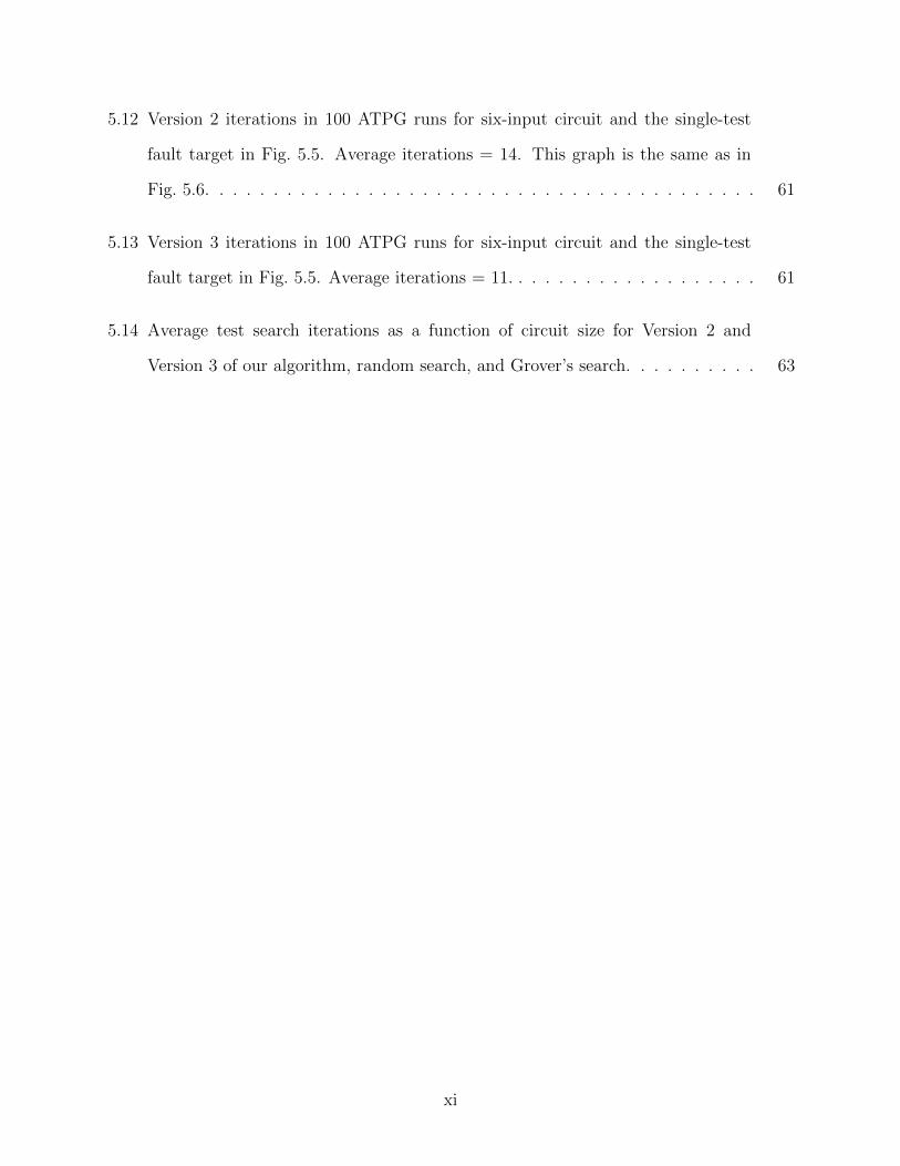
5.12 Version 2 iterations in 100 ATPG runs for six-input circuit and the single-test

fault target in Fig. 5.5. Average iterations = 14. This graph is the same as in

Fig. 5.6. . . . . . . . . . . . . . . . . . . . . . . . . . . . . . . . . . . . . . . . . 61

5.13 Version 3 iterations in 100 ATPG runs for six-input circuit and the single-test

fault target in Fig. 5.5. Average iterations = 11. . . . . . . . . . . . . . . . . . . 61

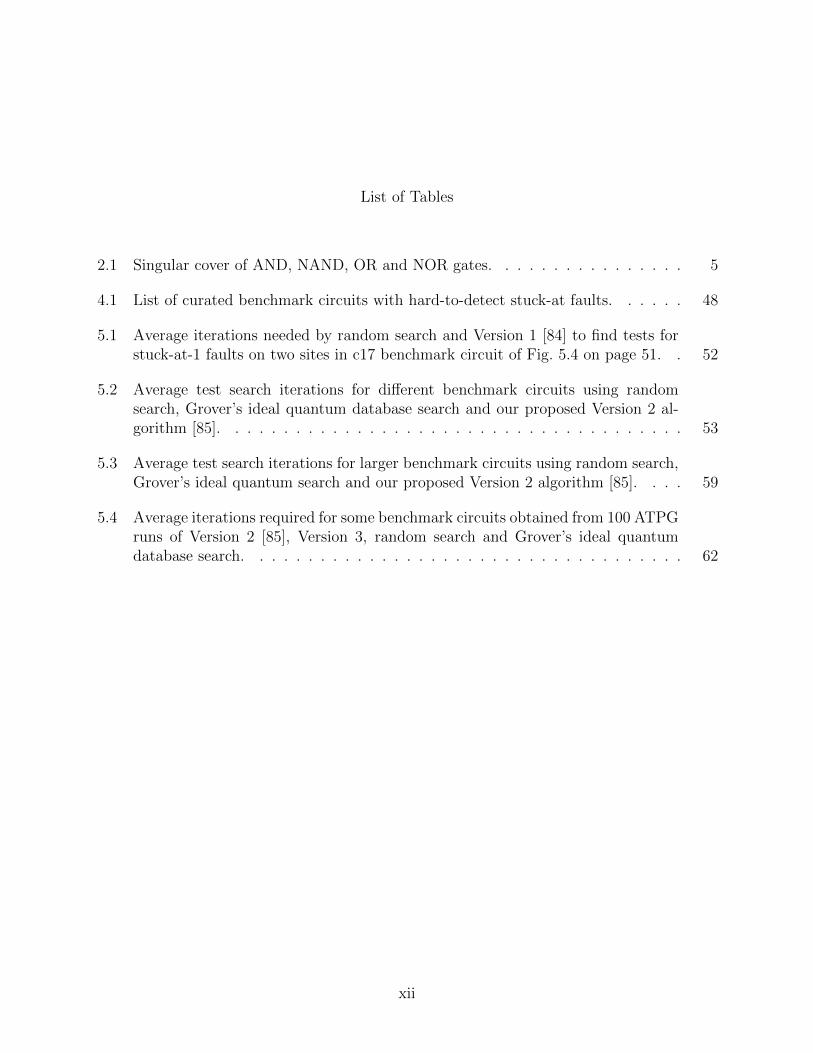
5.14 Average test search iterations as a function of circuit size for Version 2 and

Version 3 of our algorithm, random search, and Grover’s search. . . . . . . . . . 63

xi

List of Tables

2.1 Singular cover of AND, NAND, OR and NOR gates. . . . . . . . . . . . . . . . 5

4.1 List of curated benchmark circuits with hard-to-detect stuck-at faults. . . . . . 48

5.1 Average iterations needed by random search and Version 1 [84] to find tests forstuck-at-1 faults on two sites in c17 benchmark circuit of Fig. 5.4 on page 51. . 52

5.2 Average test search iterations for different benchmark circuits using randomsearch, Grover’s ideal quantum database search and our proposed Version 2 al-gorithm [85]. . . . . . . . . . . . . . . . . . . . . . . . . . . . . . . . . . . . . . 53

5.3 Average test search iterations for larger benchmark circuits using random search,Grover’s ideal quantum search and our proposed Version 2 algorithm [85]. . . . 59

5.4 Average iterations required for some benchmark circuits obtained from 100 ATPGruns of Version 2 [85], Version 3, random search and Grover’s ideal quantumdatabase search. . . . . . . . . . . . . . . . . . . . . . . . . . . . . . . . . . . . 62

xii

List of Abbreviations

ATPG Automatic Test Pattern Generation

CAVLC Context-adaptive variable-length coding

CAVLC Context-adaptive variable-length coding

CUT Circuit under Test

EDA Electronic Design Automation

FAN Fanout-Oriented Test Generation

FSM Finite State Machine

IP Intellectual Property

LGSynth Logic Synthesis and Optimization

LS-SVM Least Square Support Vector Machines

NP Non-deterministic Polynomial-time

PDF Primitive D-cubes of Failure

PI Primary Input

PO Primary Output

PODEM Path-Oriented Decision Making

RTL Register Transfer Level

SoC Silicon on Chip

xiii

TPG Test Pattern Generator

VLSI Very Large Scale Integration

xiv

Chapter 1

Introduction

The generation of test vectors is a classic VLSI testing problem. In layman’s terms, the

problem can be defined as “Given a fault, find a test.” Ever since the first digital circuit was

created, methods have been developed to test if the logic was working in the intended way.

With digital circuits becoming bigger and more complex, following the trend of Moore’s

law [56], there is a spur of interest in researching techniques for automatic test pattern

generation (ATPG) that can find tests faster and in a more efficient manner.

The testing problem has been mathematically proven to be NP complete [27, 38, 74],

leading to an increase in test generation time with an increase in circuit size and complexity.

Various test techniques have been designed and implemented to improve the test search

time. Some approaches were algorithmic [26, 31, 66, 67]; some were functional tests [5, 64];

and some used various types of weighted random test generators [3, 71] or combination

of random and algorithmic test generation [4]. Different variations of genetic algorithms

were also implemented [21, 52, 59, 68, 69]. Alternative techniques like test generation using

spectral information [90], anti-random test pattern generation [51] and energy minimization

of neural networks [16, 17], amongst others, also had their share of successes.

Over the past 50 years, there have been numerous attempts at designing more efficient

algorithms, with varying degrees of success. As is usual, because of the diminishing returns in

contemporary ATPG research, it is often claimed that the field of VLSI testing has matured

and any new research can only produce incremental rather than trailblazing progress. In

other words, the general consensus is that most major breakthroughs have been done and

the field has become saturated, with little chance of finding new algorithms.

1

Moreover, since current algorithms work by extracting new vectors based on properties

similar to previous successes, all these algorithms start hitting bottlenecks when trying to

test hard-to-detect faults that may have just a handful of unique tests in the entire search

space. It was because these hard-to-detect faults had vectors, which had different properties

as compared to previous successful vectors and hence the vector search time devolved back

to the classic NP-hard problem of VLSI testing.

Current testing algorithms have shown tremendous resilience in finding test vectors and

aiming to achieve 100% fault coverage. However, a growing interest in quantum computing

has spurred investigations in the areas of probabilistic computing algorithms [9, 12] leading

to certain problems (especially NP complete problems) being revisited to try to find optimal

solutions in linear time.

For a digital circuit with n primary inputs (PIs), the total number of test vectors, N ,

equals 2n. In other words, the search time for finding a vector to test a fault is exponential

with respect to the number of primary inputs. On an average, a simple search will take about

2n−1 iterations to find a test for a given fault. Similarly, given an unsorted database with N

elements, on average a simple search for locating a given element will take N/2 iterations,

although as we will explain, Grover’s quantum search algorithm [33] can do better.

This dissertation explains how the test generation problem can be reclassified as a

database search problem. It provides evidence on how most testing algorithms essentially use

various database search solutions and highlights the interdisciplinary connections between

the two fields. The discussion points to the need for research on test algorithms that harness

the potential of database search.

This dissertation is divided further into five more chapters. Chapter two is an overview

of ATPG research, the testing problem, and various approaches to the unsorted database

search. It highlights the connection between the two disciplines, emphasizing the need to

investigate the area of database search for a potential algorithm for VLSI test generation.

The chapter further summarizes the area of quantum computing, with a focus on the need

2

to develop quantum algorithms, and discusses applications of Grover’s algorithm [33] for

database search to the test generation problem, pointing to potential benefits.

Chapter three provides a thorough explanation of our proposed algorithm based on

our interpretation of Grover’s Algorithm of database search. The chapter expands on the

conceptual core of the proposed algorithm and provides a detailed flowchart of the algorithm’s

design.

Chapter four expands on the various tools and techniques used to conduct the exper-

iments of this dissertation. The working of electronic design automation (EDA) tools like

FastScan [25] and mathematical tools like MATLAB [55] is explained. The chapter also pro-

vides a list of various benchmark circuits used to comprehensively assess the effectiveness of

the proposed algorithms. This list has been curated from various sources and these circuits

were specifically chosen because they all have a few hard-to-detect stuck-at faults that can

only be tested by just 1-2 vectors.

Chapter five discusses the results of the experiments conducted using the methods men-

tioned in the previous chapter. A post-result analysis of the data is chronicled and using the

literature review as reference. This chapter validates the obtained results and explains the

meaning of the data obtained from the experiment.

Finally, Chapter six concludes the dissertation by summarizing all the above chapters,

elaborates on the need to search for “out of the box” solutions to the test generation problem

and suggests possible future directions of our work.

3

Chapter 2

Background

This chapter expands on key elements and research ideas from automatic test pattern

generation (ATPG) and database search. More specifically, this chapter starts off with a

thorough background history of ATPG evolution, which includes a synopsis of various types

of ATPG algorithms designed over the past 50 years. In the next section, a brief analysis of

various types of database search algorithms is provided, after which similarities in these two

seemingly unconnected fields are pointed out to the reader. The final subsection attempts to

show how advancement and research in one area can help improve the other and concludes

by expanding the virtues of quantum computing and how it can theoretically be deemed the

next step for improving the efficiency of testing algorithms.

2.1 Automatic Test Pattern Generation (ATPG)

It is colloquially understood that the test generation problem is a classic VLSI problem.

Nascent digital circuits were probably tested by running exhaustive and/or random tests as

the circuit sizes were quite small. However, exhaustive/random testing became horribly inef-

ficient for larger circuits. Research has firmly established that the fault detection problem is

NP-complete [27, 38, 74]. The nature of an NP-complete problem implies that increasing the

circuit size will exponentially increase the worst case computation time for test generation.

These issues quickly led to development of algorithms that can derive test vectors for

modeled fault targets, using the structural description of a circuit. Three of the well-known

algorithms initially developed are the D-algorithm [66, 67], PODEM [31] and FAN [26]. The

following subsections expand on each algorithm in greater detail.

4

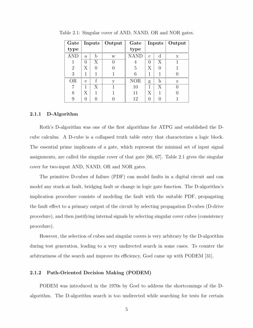
Table 2.1: Singular cover of AND, NAND, OR and NOR gates.

Gate Inputs Output Gate Inputs Outputtype type

AND a b w NAND c d x1 0 X 0 4 0 X 12 X 0 0 5 X 0 13 1 1 1 6 1 1 0

OR e f y NOR g h z7 1 X 1 10 1 X 08 X 1 1 11 X 1 09 0 0 0 12 0 0 1

2.1.1 D-Algorithm

Roth’s D-algorithm was one of the first algorithms for ATPG and established the D-

cube calculus. A D-cube is a collapsed truth table entry that characterizes a logic block.

The essential prime implicants of a gate, which represent the minimal set of input signal

assignments, are called the singular cover of that gate [66, 67]. Table 2.1 gives the singular

cover for two-input AND, NAND, OR and NOR gates.

The primitive D-cubes of failure (PDF) can model faults in a digital circuit and can

model any stuck-at fault, bridging fault or change in logic gate function. The D-algorithm’s

implication procedure consists of modeling the fault with the suitable PDF, propagating

the fault effect to a primary output of the circuit by selecting propagation D-cubes (D-drive

procedure), and then justifying internal signals by selecting singular cover cubes (consistency

procedure).

However, the selection of cubes and singular covers is very arbitrary by the D-algorithm

during test generation, leading to a very undirected search in some cases. To counter the

arbitrariness of the search and improve its efficiency, Goel came up with PODEM [31].

2.1.2 Path-Oriented Decision Making (PODEM)

PODEM was introduced in the 1970s by Goel to address the shortcomings of the D-

algorithm. The D-algorithm search is too undirected while searching for tests for certain

5

Start

Assign a binary valueto an unassigned PI

Determine implications of all PIs

Is a testgenerated?

Exit: Done

Test possiblewith additionalassigned PIs?

Is there an un-tried combination

of values onassigned PIs?

Choose objectives, performbacktrace and set untried combi-nation of values on assigned PIs

Exit: Untestablefault

Yes

No

Maybe

No

Yes

No

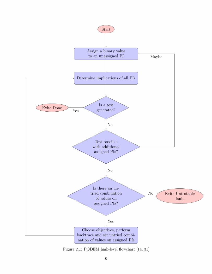
Figure 2.1: PODEM high-level flowchart [14, 31]

6

circuits (e.g., DRAM memory) [14]. The authors of [14] published a flow chart of a typical

PODEM algorithm, which is given in Figure 2.1.

Some of PODEM’s important properties that distinguish it from the D-algorithm are:

• PODEM’s primary objective is to ensure the propagation of a D or D to a primary

output (PO) .

• PODEM introduced the concept of backtrack to accelerate the search. A subroutine

would check whether the D-frontier disappeared and if so, would backtrack immediately

to attempt a different path.

• PODEM’s binary decision tree is centered around the primary input variables and not

around all circuit signals. Hence, the search tree size changes from 2n, where n is the

number of logic gates and primary inputs to 2#PIs, where #PIs is number of primary

inputs.

The concepts of PODEM were further refined by Fujiwara and Shimono in their fanout-

oriented test generation (FAN) algorithm [26] and are discussed in detail in the next subsec-

tion.

2.1.3 Fanout-Oriented Test Generation (FAN)

PODEM also encounters a number of inefficiencies. Fujiwara and Shimono developed

FAN algorithm [26] to further improve upon the concept of test search pioneered by PODEM,

especially in four particular areas [14]:

• Immediate Implications: PODEM sometimes misses situations where it can im-

mediately assign values to certain signals. For example, if a circuit has a three input

NAND gate and the output of the NAND gate is a value 0 to be backtraced to the PIs,

PODEM would assign one of the inputs to the NAND gate as a 1 and backtrace it.

This backtrace, which is immediately followed by forward implication, can erroneously

7

assign 0 to either of the two inputs before correcting itself. If FAN were presented with

the same situation, it would automatically assign 1 to all three inputs.

• Unique Sensitization: In certain cases, it is possible that a fault can propagate

through only one path to POs. In that condition, it is viable to sensitize these paths

for propagation by setting the other signals for propagation immediately, rather than

wait for the values to be assigned during search. This is another opportunity to improve

search time.

• Headlines: Headlines are defined as certain lines in the circuit which, if cut or discon-

nected, can isolate a logic section (or cone of logic) driven by PIs from the rest of the

digital circuit. The primary advantage of headlines is that a cone of logic representing

a section of PIs can be removed and replaced with one choice for the headline. The

signal assignments for the PIs feeding the headline are deferred for a later time until

the search algorithm has viable assignments.

• Multiple Backtrace: This is the final improvement of FAN over PODEM. PODEM’s

backtrace works in a depth-first fashion. In certain cases, this process is laborious and

very inefficient. FAN addresses this by backtracing in a breadth-first fashion. This

method can find a signal conflict faster than a single backtrace procedure (like in

PODEM), quickly find the decision creating said conflict, and reverse it faster than

PODEM.

Those described above and many later algorithms, like SOCRATES [73], non-heuristic [36],

or learning [46], approaches vastly improved search time over random and exhaustive test

pattern generators (TPG).

During the 1970s, other avenues of deriving test vectors were explored as well. Manu-

facturers needed a way to protect their intellectual property (IP) but needed ways to test

their circuits as well. This spurred research interest in deriving test sets from functional

descriptions of circuits rather than circuit structure [5, 64]. The derivation of “universal

8

test sets” was useful because they could be applied to multiple implementations of the same

logic.

Akers’ paper tackles the problem of deriving a single universal test set to test any

implementation of a switching network [5]. His paper showed that these “universal tests”

have a number of desirable features like:

• Ease of test generation using truth table or algebraic procedures.

• Can be applied to multiple implementations of a switching network.

• Can guarantee coverage of all single and multiple faults.

• Can be derived for single and multiple output functions or for both complete and

incomplete functions.

Reddy also tackles the problem of deriving tests from functional descriptions rather than

structural description of circuits [64]. His work introduces the concept of an expanded truth

table for logic networks. The paper proved that the set of minimal true vertices and maximal

false vertices of the expanded truth table constitutes a test set to detect any number of stuck-

at-faults in a unate gate network. These test sets can remain valid even in the presence of

redundancies in the logic network [64].

However, there are certain downsides to these universal test sets as well [5]. They can

only work for monotonic circuits or specially designed circuits like and/or network imple-

mentations, which can be less than optimal. They always contain more tests than required

(because of the nature of the universal test sets) as they need to cover all implementations

of a circuit logic. In certain cases, the may cover all possible inputs, which can become

exhaustive and impractical.

Another avenue of research thoroughly investigated was the design of weighted random

test generators. Schnurmann et al.’s work provided a significant departure from deterministic

algorithms [71]. They postulated that since not all PIs have the same functional importance,

9

devising a technique to exercise some PIs more than others would yield significant results. PIs

were selected using heuristics like increased input switching activity and weight assignment

to PIs in order to derive new test sets [71]. Weighted random vectors were investigated by

several other researchers [1, 60].

This work was one of the earliest which significantly departed from classical or algo-

rithmic methods of test generation. Their results showed high testability numbers of their

weighted random TPG even when circuits had complex components like counters or shift

registers. Their paper also elucidates that their method can be applied to both ATPG or

BIST circuitry without any loss in test coverage [71].

Another version of weighted random test generator applied the concept of information

theory to the problem of testing digital circuits [3]. Agrawal analyzed the information

throughput in the circuit and derived an expression for the probability of detecting a fault

in the hardware. Using the example of a simple 10-input AND gate, his paper explains

how modifying the design of a test pattern generator can yield significant results. More

specifically, the paper skewed the input probability in such a manner so that maximum

output entropy is attained [3]. In other words, the test vectors were derived from those

input combinations which caused most output transitions. Agrawal’s results concluded on

the qualitative importance of designing test pattern generators to indicate high probability of

fault detection using statistical information properties. The paper highlights applications in

testing of faults in analog circuits and use of problem-specific information to create random

patterns for software testing.

When these algorithms started hitting their limits, there were forays into non-traditional

implementations that further improved test coverage. An alternative method [17] converts

a digital circuit into a neural network such that a test vector represents a minimum energy

state. Essentially, the testing problem is rephrased as an energy minimization problem. A

test is obtained by determining signal values satisfying a Boolean equation from the neural

network as long they are activating the fault and sensitizing the path.

10

Chakradhar et al.’s work highlighted several advantages over conventional algorithms [17].

Instead of using multiple approaches for branch-and-bound search, only a single tool in the

form of transitive closure is required. Their method can also determine signal relationships in

the circuit and calculate all logical consequences based on signal pair relationships for a par-

tial set of signal assignments. They also hypothesize that their work is easily parallelizable

and can be included in any test generation algorithm and extend their efficiency.

Malaiya [51] introduced the concept of anti-random testing. This strategy used Ham-

ming distance and/or Cartesian distance measures to derive new vectors from previously

known successful vectors. This idea was introduced to formally define how to utilize infor-

mation of previous tests to generate more tests. Essentially, this is a black-box approach to

maximize the effectiveness of test vectors by trying to keep tests as different as possible from

each other.

Cheng and Agrawal devised a new simulation-based method that can derive new tests

by minimizing a “cost function” [18]. This algorithm calculates a “cost function” after

generating a vector and running a simulation. If the cost is deemed high (based on a

threshold margin), the vector is not a test and changes in the vector are made in an attempt

to reduce the cost function. One of the major advantages of this algorithm is that there is no

need of any explicit backtracking. Their research results show that the performance exceeds

that of conventional test generation tools. Because of the simple implementation, this work

can be easily incorporated in any fault simulation program without any major changes.

Similarly, genetic algorithms define a “fitness function” for choosing vectors with high

fitness [21, 52, 59, 68, 69]. There are two major advantages of genetic algorithms. They can

be used for fast test vector generation. Secondly, their topological nature enables the ATPG

to escape local minima and identify untestable faults. The fitness value assigned to a test

determines its probability of selection as a parent; the higher the fitness value the greater

the probability of the test being selected to engage in reproduction. Reproduction means

modifying the parent test vector to generate more test vectors for other fault sites [59].

11

Looking at the research trend, it is clearly seen that ATPG algorithm methodologies

have been leaning toward extracting new tests based on previous successes. One of the

more contemporary techniques was devised by Yogi and Agrawal [90]. Their method uses

Hadamard matrices to analyze Walsh function spectrum of previously successful vectors to

generate new vectors [90]. The authors generated test vectors for Register Transfer Level

(RTL) faults and analyzed then using a Hadamard matrix to extract important features,

after which new vectors are generated retaining those features. According to Yogi and

Agrawal, this technique is found to be an efficient and reliable method for test generation.

Their results show that as circuits become larger the RTL method may have advantages

over gate-level ATPG, revealing a potential in generation of test vectors at RTL by spectral

analysis.

With chip sizes shrinking and device density growing, test power has become a concern

as well. Early solutions talked about reordering of test vectors to reduce the number of

transitions. Girard et al. [29] attempted to minimize average and peak power dissipation

during test operation. Their proposed technique was to reduce the internal switching activity

by lowering the transition density at circuit inputs. Their experimental results showed a

reduction in switching activity between 11% and 66% during test application. Later, more

rigorous solutions were implemented such as adaptive clock cycles [83] and dynamic voltage

and frequency scaling for System on Chips (SoC) [75].

These paragraphs give just a small snapshot of the research trend in VLSI testing over

the past 50 years. A comprehensive list of all publications in this field would be longer than

the length of this dissertation. It is interesting to note that whenever bottlenecks appeared

in “traditional algorithms” of the day, solutions were found by “out of the box” thinking.

These 50 years of research have helped fine-tune many commercial tools offered by

electronic design automation (EDA) companies like Cadence [15], Mentor Graphics [53] and

Synopsys [82]. Because of the efficiency of these tools and the time spent in perfecting them,

there are claims that ATPG research has reached its maturity. However, in spite of these

12

claims, we remain optimistic that new solutions can be found by venturing outside the box

again and looking for solutions, sometimes in a totally orthogonal research field.

2.2 Database Search Algorithms

It is fairly obvious that searching through a sorted database is faster than searching

through an unsorted database. Given a problem to find an element in a sorted database

of N elements, the solution to that is a straightforward application of a divide and conquer

algorithm called the “binary search” [44]. It is performed by comparing the target value

with the middle element of the database. If the middle element matches the target value,

the index is returned. If the target value is smaller than the current position, the search

continues in the lower half of the database else it continues in the upper half.

Because of the ease of searching a sorted database, it can be deemed convenient to sort

an unsorted database before searching for the element. However, the complexity of sorting

a database increases exponentially with increasing database size, along with the need for a

large swap memory. Hence, there arises a need to find solutions to search through unsorted

databases as efficiently as possible.

The simplest search algorithm which can check the database for an element until it is

found or the list is exhausted is “linear search”. However, in the worst case we must iterate

through the entire database and hence it can be computationally expensive. One easy way

to improve linear search speed is to break up the database into smaller segments and then

search through the sections in a parallel fashion. However, even this parallel approach has

its limits, as highlighted by Amdahl’s law [8]. More efficient search algorithms like tree

traversal, simulated annealing, and genetic algorithms, among countless others, can also be

parallelized to achieve faster results.

Tree traversal is a type of database search referring to the process of visiting each

element in a tree database at least once, systematically. There are two major approaches to

tree traversal: depth-first and breadth-first. Depth first search implies starting at the root

13

of the tree and exploring as far as possible to a final leaf before backtracking and trying a

different path. Breadth first search starts at the root of the tree and explores all neighbors

at a given depth level before heading down to the next level.

Simulated annealing is an offshoot of statistical mechanics in which a sequence of iter-

ations is performed starting from an initial configuration [43]. After each iteration, a new

configuration is selected from the neighborhood of the old one and variations in the cost

function are compared. Depending upon the value of the cost function, the transition is

either accepted or rejected, according to a predefined probability function.

Genetic algorithms perform a search by mimicking the process of natural selection [32,

54]. Each element is assigned a fitness value based on an evaluation function. The higher the

fitness value, the closer the element to the optimal solution. During each selection process,

elements with higher fitness values are selected to create the next set. By utilizing tech-

niques from natural selection like inheritance, mutation, selection, etc., genetic algorithms

can generate solutions to optimization and search problems.

2.3 Interdisciplinary Connection

Although we discussed VLSI Testing and database search, this work does not provide a

detailed literature review of either field. The primary reason for covering the key elements in

both areas is to show how the testing problem can be redefined as a database search problem

and how various testing algorithms are essentially iterations of database search algorithms.

Given a digital circuit with n primary inputs, the database of vectors can have 2n = N

possible vector combinations. A fault in this circuit must be tested by at least one of these

possible vectors. Applying brute force in trying to find a test using random test generators

is analogous to a linear search of a database. If the circuit is large, the search will be

horribly inefficient. To counter this inefficiency, the earliest algorithms, D-algorithm [66]

and PODEM [31], were essentially versions of tree traversal. While the D-algorithm is

analogous to a breadth-first search, PODEM has its roots in depth-first search.

14

Some weighted random test generators [3, 71], antirandom testing [51] and spectral test

generation [90] are forms of simulated annealing. These algorithms generate new tests based

on previous successful tests and are dependent on some sort of cost function. There have

also been direct applications of genetic algorithms in testing [21, 59, 68, 69].

These comparisons essentially emphasize the fact that testing algorithms can be re-

classified as a database search problem. Hence, it would be hugely beneficial if an ATPG

algorithm was developed which utilized one of the most efficient database search algorithms.

In other words, an ATPG implementation of “Grover’s algorithm for database search” [33]

would break the current plateau of research in VLSI testing. Being a quantum algorithm, the

speed-up is significant compared to other classic algorithms and has been mathematically

proven to be the most optimal [13].

2.4 Quantum Computing - The Future!

Quantum computing has been touted as a “silver bullet” solution to many research

problems of exponential complexity [22]. It can have wide ranging applications [58] extending

from quantum information processing (QIP) like quantum simulations [19, 47] or quantum

communication [42] to quantum cryptography [11, 24, 30] or quantum modeling [88]. The

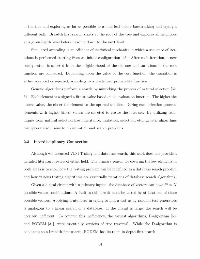
authors in [23] highlight seven stages towards building a practical quantum computer. The

pictorial representation from their paper has been reproduced in Fig. 2.2 on the following

page.

Although the stages in this complexity versus time graph overlap and are interconnected,

advancement to the top requires not only mastery of each stage but continuous perfecting of

each stage in parallel to the others. According to the authors, the green arrow in 2.2 indicates

the aim at reaching the fourth stage as current research is presently at stage three. Currently,

there is a lot of research interest in trying to develop quantum circuits. These circuits are

being built on detailed reviews of the principles discussed in previous research [20, 72].

15

Figure 2.2: Seven stages of developing of a practical quantum computer [23].

Recently, scientists have been successful in building a quantum logic gate in silicon that can

form the building block of a working quantum computer [63].

Successful entangling of three-circuit systems have already improved the prospects for

solid-state quantum computing [65]. Research has progressed to such an extent that there

is a commercial quantum computing company set up (called D-wave) [40]. D-wave has seen

its share of success and their quantum computers are being extensively used by Google

and NASA for their research [41]. Recently, IBM scientists have reported critical advances

towards building a practical quantum computer. They showed a new quantum circuit design

that may easily scale to larger dimensions along with showing an ability to measure and detect

different types of quantum errors simultaneously [62]. In spite of all these developments,

materials, circuit design and manufacturing technologies must advance. Until then real

large scale quantum computing would remain a phenomenon of the future, not too distant

we hope [48].

However, building of quantum computers alone is not enough. In order to test if the

quantum computer is indeed working as it was designed, there need to be algorithms which

16

can properly make use of the quantum properties, aka quantum algorithms. One of the

most popular quantum algorithms used to test quantum circuits is Shor’s algorithm for

factorization [76]. This algorithm can solve the following problem in linear time, “Given

an integer N , find its prime factors”. Solving a problem of this magnitude (which has

exponential complexity) can be a huge boost to the world of computing.

Another algorithm which is quite popular among researchers is Grover’s algorithm for

database search [34]. There is keen interest in the scientific community to apply this al-

gorithm in their respective fields, potentially producing dramatic speed-ups. Furthermore,

it has been mathematically shown that Grover’s algorithm is optimal. In other words, any

algorithm that can successfully access a database must run at least as many iterations as

Grover’s algorithm [13]. The way Grover’s algorithm finds an answer is very simple and

elegant and it is properly elaborated in the following section.

2.5 Grover’s Algorithm - A Possible Solution

Grover’s algorithm searches an unordered database of N items to find a specified item.

Its quantum search is quadratically faster than any other classical search algorithm [33, 34].

Its complexity is O(√N), as compared to classical algorithms with complexity ranging from

O(N) to O(logN) [13].

Understanding Grover’s algorithm isn’t the most intuitive process because it uses fun-

damental concepts of quantum mechanics. However, we will attempt to give a very holistic

view of how it works. The key concept of the algorithm is that instead of checking possible

solutions one by one, a uniform superposition is created over all possible solutions and then

a quantum operation destructively interferes with all the states that are NOT solutions in a

repeated fashion until the correct solution can be gleaned with high probability.

In a search space of N elements (or 2n vectors), the focus of search is concentrated

on the index of the elements rather than the elements themselves. The search problem is

17

redefined as a function f , which takes an integer x in the range 0 to N − 1. Hence, f(x) = 1

if x is a solution to the search problem and f(x) = 0 if x is not a solution [58].

Grover’s algorithm introduces a concept of a quantum black box, called Oracle , whose

internal workings are not defined but termed problem-specific [34]. The oracle has the ability

to recognize a solution without knowing the solution. The authors in [58] highlight a crucial

point that it is possible to do the former without necessarily doing the latter. In other words,

the oracle does not know the solution itself but knows the properties of the solution and can

identify it when shown.

A lot of resources have thoroughly explained the working of Grover’s algorithm using

animated GIFs [28] or worked out examples [81]. The steps/iterations of Grover’s algorithm

are elegantly summarized below [58]:

• Apply the Oracle.

• Apply the Hadamard transform.

• Perform a conditional phase shift with every possible state except the initial state

receiving a phase shift π.

• Apply the Hadamard transform.

Grover iterations are regarded as a rotation in the two-dimension space spanned by the

starting vector and the superposition of all possible solutions to the search problem. If α

indicates a sum where x are not solutions to the search problem, and β indicates sum of x

which are solutions, the oracle performs a reflection about the vector α in the plane defined

by α and β. The correct solution rotates by an angle of θ after each iteration and after

enough Grover iterations, the solution approaches the value of β.

Because of the quantum speed-up provided by Grover’s algorithm, it would be highly

beneficial to find a working application in VLSI testing. Furthermore, there have been

claims of Grover’s algorithm being able to solve the Boolean satisfiability problem in O(√N)

18

time [7]. The next section presents key elements of a few papers that have attempted to

create new testing algorithms based on Grover’s algorithm.

2.6 Application of Grover’s Algorithm in ATPG

There have been attempts at applying Grover’s algorithm to find test vectors for VLSI

circuits. Authors in [78] and [77] used formulation of Chakradhar et al. [16] as a starting

point by reclassifying the testing problem as an energy minimization problem of a neural

network. By converting the circuit to a neural network, they showed [78] that it is possible

to use Grover’s algorithm to successfully find a test vector faster than other methods like

simulated annealing or exhaustive search. While these authors did not elaborate on the

type of circuits on which they got their results or provide a detailed explanation of their

procedure, a general proof of concept was established for other researchers to work on.

The authors of [77] published a more comprehensive study with a detailed analysis of

ISCAS’89 benchmark circuits. They compared their implementation of Grover’s algorithm,

called QATPG, with a DNA based algorithm DATPG, genetic algorithm and exhaustive

search. We reproduce two interesting graphs to highlight the underlying theme of the paper.

Fig. 2.3 compares the number of iterations required to find a test by performing an

exhaustive search vs. quantum search. Note that while there is an exponential increase in

search time with increasing circuit size when performing exhaustive search, the quantum

search (Grover’s algorithm) increases almost linearly. This is consistent with the underlying

theory established so far and further emphasizes the proof of concept of Grover’s algorithm.

Fig. 2.4 takes the case of the largest circuit requiring 25 neurons (N = 2n possible

vectors) and compares the CPU time required to attain 100% fault coverage. While none

of the algorithms is able to detect all faults, it is interesting to see that quantum search

(QATPG) attains the highest fault coverage within the least CPU time whereas exhaustive

search (ES) gets the least fault coverage while taking the longest time.

19

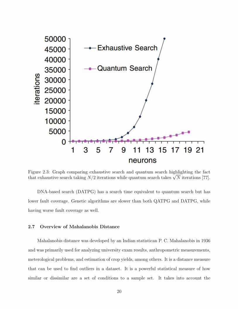
Figure 2.3: Graph comparing exhaustive search and quantum search highlighting the factthat exhaustive search taking N/2 iterations while quantum search takes

√N iterations [77].

DNA-based search (DATPG) has a search time equivalent to quantum search but has

lower fault coverage. Genetic algorithms are slower than both QATPG and DATPG, while

having worse fault coverage as well.

2.7 Overview of Mahalanobis Distance

Mahalanobis distance was developed by an Indian statistican P. C. Mahalanobis in 1936

and was primarily used for analyzing university exam results, anthropometric measurements,

meterological problems, and estimation of crop yields, among others. It is a distance measure

that can be used to find outliers in a dataset. It is a powerful statistical measure of how

similar or dissimilar are a set of conditions to a sample set. It takes into account the

20

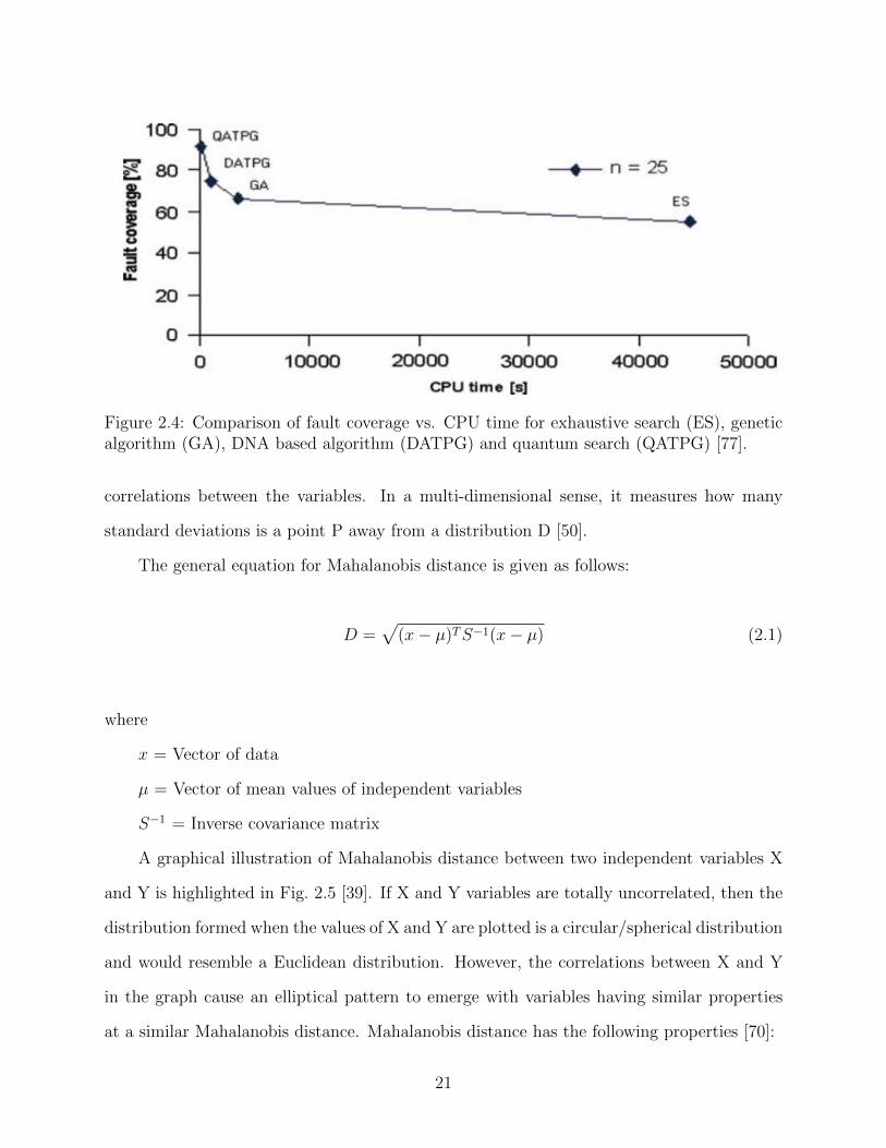
Figure 2.4: Comparison of fault coverage vs. CPU time for exhaustive search (ES), geneticalgorithm (GA), DNA based algorithm (DATPG) and quantum search (QATPG) [77].

correlations between the variables. In a multi-dimensional sense, it measures how many

standard deviations is a point P away from a distribution D [50].

The general equation for Mahalanobis distance is given as follows:

D =√

(x− µ)TS−1(x− µ) (2.1)

where

x = Vector of data

µ = Vector of mean values of independent variables

S−1 = Inverse covariance matrix

A graphical illustration of Mahalanobis distance between two independent variables X

and Y is highlighted in Fig. 2.5 [39]. If X and Y variables are totally uncorrelated, then the

distribution formed when the values of X and Y are plotted is a circular/spherical distribution

and would resemble a Euclidean distribution. However, the correlations between X and Y

in the graph cause an elliptical pattern to emerge with variables having similar properties

at a similar Mahalanobis distance. Mahalanobis distance has the following properties [70]:

21

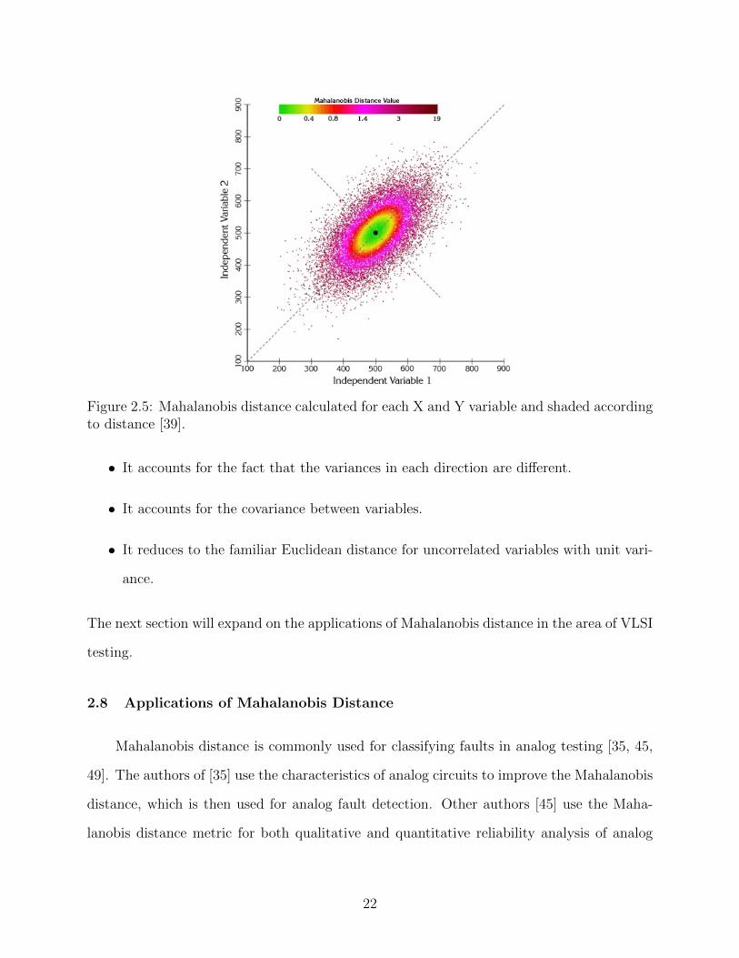
Figure 2.5: Mahalanobis distance calculated for each X and Y variable and shaded accordingto distance [39].

• It accounts for the fact that the variances in each direction are different.

• It accounts for the covariance between variables.

• It reduces to the familiar Euclidean distance for uncorrelated variables with unit vari-

ance.

The next section will expand on the applications of Mahalanobis distance in the area of VLSI

testing.

2.8 Applications of Mahalanobis Distance

Mahalanobis distance is commonly used for classifying faults in analog testing [35, 45,

49]. The authors of [35] use the characteristics of analog circuits to improve the Mahalanobis

distance, which is then used for analog fault detection. Other authors [45] use the Maha-

lanobis distance metric for both qualitative and quantitative reliability analysis of analog

22

electronic devices. Another group [49] used Mahalanobis distance to design least square

support vector machines (LS-SVM) for analog circuit diagnostics.

The technique has also been used for multi-dimensional Iddq testing [57], analysis of

the wavelet energies for mixed-signal testing [80] and generating diagnostic programs for

mixed-signal load boards [61]. However, the Mahalanobis distance metric has never been

used to derive tests for stuck-at faults. A recent paper [87] suggests utilizing this technique

for targeting specific hard-to-detect stuck-at faults that may only have a couple of tests in

the entire test vector space.

Intuitively, it can be understood that in order to find a vector to test a fault, it is

imperative to “move away” from the failed (unsuitable) vector region and towards acti-

vation/propagation vector territories. If each primary input has been initialized to a 0.50

probability of ‘1’ or ‘0’, the weights have to be modified such that the distance of a generated

trial vector is maximum from the mean of the failed vector distribution.

The concept outlined above can be implemented in a variety of ways or techniques.

This dissertation proposes that if a certain probability weights at PIs generate logic values

(1 or 0) in a vector, which neither activates the fault nor sensitizes a path to POs, it is

best to modify the weights in such a manner that the failed vectors’ Mahalanobis distance is

maximized before generating new vectors. This method is repeated until the search enters

the region of activation and/or propagation vectors.

Once the search enters either of these regions, it is in our best interest that the search

does not deviate away from this vector subspace and hence modifications to the probability

weights are made in smaller increments. Since the correlation between the PIs is also taken

into consideration (via the inverse covariance matrix) while calculating the distance metric,

the algorithm is self-tuning and the search gets skewed toward the correct test vector.

23

Chapter 3

Algorithm Design

The genesis of our algorithm started by asking a very philosophical question: “How does

one prosper in life?” In general, there are two steps in trying to answer this question:

• As people say, do not change a successful formula. So, it is wise to keep repeating steps

from previous successes.

• Learning from past failure and avoiding steps which caused those failures.

From our analysis of contemporary testing algorithms (provided in the literature review

of Section 2.1), it is seen that these algorithms use only previous successes to generate

new test vectors. However, test generation usually has a lot more failed attempts than suc-

cessful ones, especially for hard-to-detect stuck-at faults with only one or two test vectors.

It is known that there is a strong correlation among the input bits of test vectors applied

at the primary inputs (PIs) [5]. Contemporary testing algorithms extract new test vectors

based on properties similar to previous successes or try to arrive at the solution in a de-

terministic manner by trying to propagate a fault to the primary outputs (POs). All these

algorithms ignore the failed test vectors and hence are throwing away lots of potentially

useful information, which can help deduce the solution faster.

We attempt to answer the question: “How to design a new test algorithm that

utilizes the information from failed attempts effectively?” We developed three algo-

rithms, each one an enhanced version of the previous one in order to improve the search for

a test vector to detect a given stuck-at fault.

24

3.1 Version 1

The fundamental principle behind this algorithm is that there are correlations present

among the bits of a test vector applied at the primary inputs [5]. In other words, during test

generation, if a bit is a ‘0’ at a particular input, we can predict, with a certain probability,

the state of the other bits at the other primary inputs. We aim to quantify these correlations

in an n× n matrix of conditional probabilities (where n is the number of primary inputs to

a circuit). The diagonal values represent the independent probabilities of a state being a ‘0’

or a ‘1’ at the primary inputs, whereas the off-diagonal elements represent the conditional

probabilities of the input vector bits given deterministic values for other bits.

This method will improve the search of test vectors for stuck-at faults in the following

manner [84]:

1. When the test vector search hits the bottleneck caused by hard-to-detect stuck-at

faults, our conjecture is that we need to try vectors whose properties are not similar to

the current probability correlation matrix (built out of previously used test vectors).

In colloquial terms, we aim to avoid the vectors that share the characteristics of the

unsuccessful vectors.

2. By statistically reducing the probability of choosing test vectors that share properties

similar to the previously known unsuccessful vectors, we aim to skew the search in the

test vector space toward the correct test vector which can trigger the fault, based on

the conjecture described above.

3. The correlation matrix contains information of unsuccessful test vectors of hard-to-

find stuck-at faults and we can use the opposite correlation to extract the right test

vectors, which will test the hard-to-detect faults, in a time faster than random search

algorithms. The vector set extracted by the above algorithm should take fewer itera-

tions when compared to a random vector search.

25

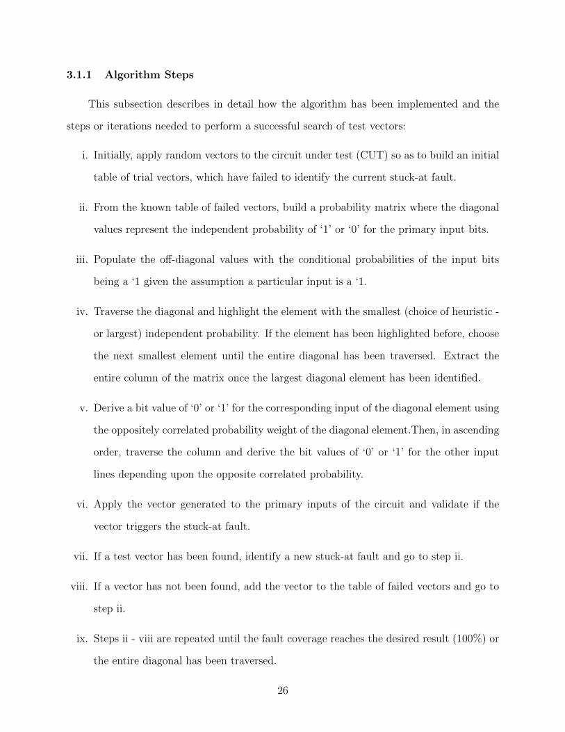
3.1.1 Algorithm Steps

This subsection describes in detail how the algorithm has been implemented and the

steps or iterations needed to perform a successful search of test vectors:

i. Initially, apply random vectors to the circuit under test (CUT) so as to build an initial

table of trial vectors, which have failed to identify the current stuck-at fault.

ii. From the known table of failed vectors, build a probability matrix where the diagonal

values represent the independent probability of ‘1’ or ‘0’ for the primary input bits.

iii. Populate the off-diagonal values with the conditional probabilities of the input bits

being a ‘1 given the assumption a particular input is a ‘1.

iv. Traverse the diagonal and highlight the element with the smallest (choice of heuristic -

or largest) independent probability. If the element has been highlighted before, choose

the next smallest element until the entire diagonal has been traversed. Extract the

entire column of the matrix once the largest diagonal element has been identified.

v. Derive a bit value of ‘0’ or ‘1’ for the corresponding input of the diagonal element using

the oppositely correlated probability weight of the diagonal element.Then, in ascending

order, traverse the column and derive the bit values of ‘0’ or ‘1’ for the other input

lines depending upon the opposite correlated probability.

vi. Apply the vector generated to the primary inputs of the circuit and validate if the

vector triggers the stuck-at fault.

vii. If a test vector has been found, identify a new stuck-at fault and go to step ii.

viii. If a vector has not been found, add the vector to the table of failed vectors and go to

step ii.

ix. Steps ii - viii are repeated until the fault coverage reaches the desired result (100%) or

the entire diagonal has been traversed.

26

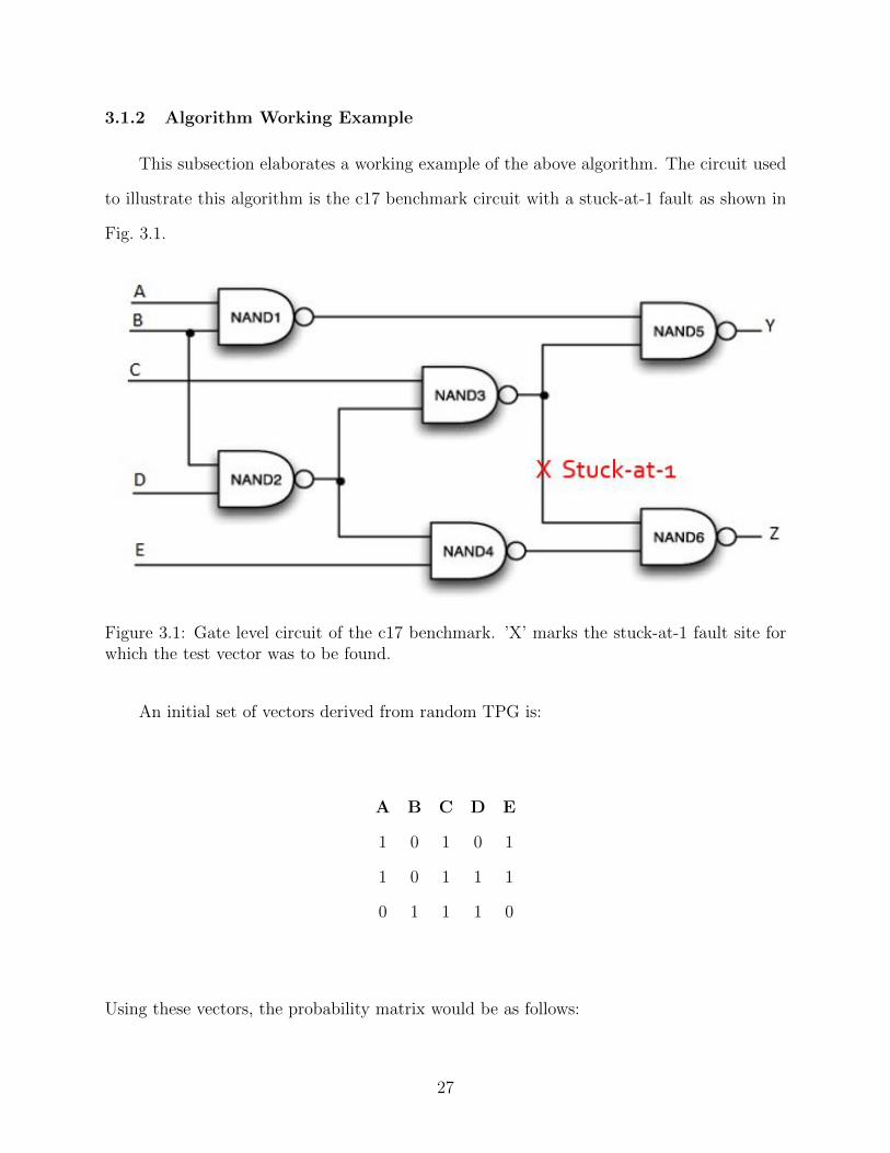
3.1.2 Algorithm Working Example

This subsection elaborates a working example of the above algorithm. The circuit used

to illustrate this algorithm is the c17 benchmark circuit with a stuck-at-1 fault as shown in

Fig. 3.1.

Figure 3.1: Gate level circuit of the c17 benchmark. ’X’ marks the stuck-at-1 fault site forwhich the test vector was to be found.

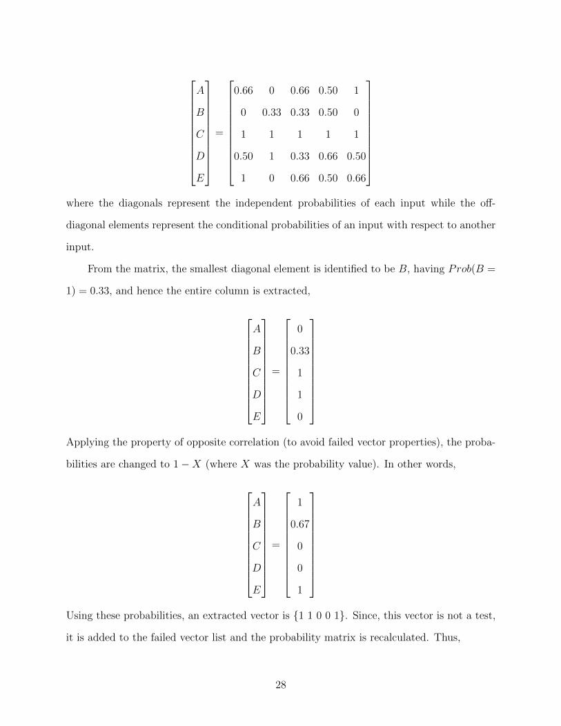
An initial set of vectors derived from random TPG is:

A B C D E

1 0 1 0 1

1 0 1 1 1

0 1 1 1 0

Using these vectors, the probability matrix would be as follows:

27

A

B

C

D

E

=

0.66 0 0.66 0.50 1

0 0.33 0.33 0.50 0

1 1 1 1 1

0.50 1 0.33 0.66 0.50

1 0 0.66 0.50 0.66

where the diagonals represent the independent probabilities of each input while the off-

diagonal elements represent the conditional probabilities of an input with respect to another

input.

From the matrix, the smallest diagonal element is identified to be B, having Prob(B =

1) = 0.33, and hence the entire column is extracted,

A

B

C

D

E

=

0

0.33

1

1

0

Applying the property of opposite correlation (to avoid failed vector properties), the proba-

bilities are changed to 1−X (where X was the probability value). In other words,

A

B

C

D

E

=

1

0.67

0

0

1

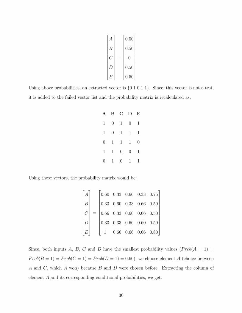
Using these probabilities, an extracted vector is {1 1 0 0 1}. Since, this vector is not a test,

it is added to the failed vector list and the probability matrix is recalculated. Thus,

28

A B C D E

1 0 1 0 1

1 0 1 1 1

0 1 1 1 0

1 1 0 0 1

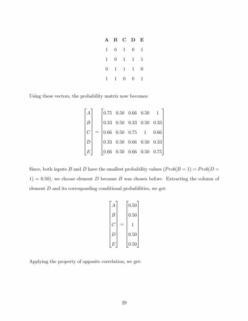
Using these vectors, the probability matrix now becomes:

A

B

C

D

E

=

0.75 0.50 0.66 0.50 1

0.33 0.50 0.33 0.50 0.33

0.66 0.50 0.75 1 0.66

0.33 0.50 0.66 0.50 0.33

0.66 0.50 0.66 0.50 0.75

Since, both inputs B and D have the smallest probability values (Prob(B = 1) = Prob(D =

1) = 0.50), we choose element D because B was chosen before. Extracting the column of

element D and its corresponding conditional probabilities, we get:

A

B

C

D

E

=

0.50

0.50

1

0.50

0.50

Applying the property of opposite correlation, we get:

29

A

B

C

D

E

=

0.50

0.50

0

0.50

0.50

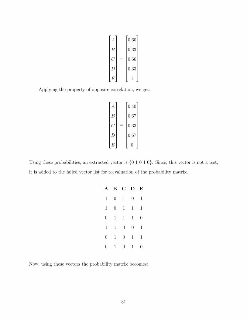
Using above probabilities, an extracted vector is {0 1 0 1 1}. Since, this vector is not a test,

it is added to the failed vector list and the probability matrix is recalculated as,

A B C D E

1 0 1 0 1

1 0 1 1 1

0 1 1 1 0

1 1 0 0 1

0 1 0 1 1

Using these vectors, the probability matrix would be:

A

B

C

D

E

=

0.60 0.33 0.66 0.33 0.75

0.33 0.60 0.33 0.66 0.50

0.66 0.33 0.60 0.66 0.50

0.33 0.33 0.66 0.60 0.50

1 0.66 0.66 0.66 0.80

Since, both inputs A, B, C and D have the smallest probability values (Prob(A = 1) =

Prob(B = 1) = Prob(C = 1) = Prob(D = 1) = 0.60), we choose element A (choice between

A and C, which A won) because B and D were chosen before. Extracting the column of

element A and its corresponding conditional probabilities, we get:

30

A

B

C

D

E

=

0.60

0.33

0.66

0.33

1


A

B

C

D

E

=

0.40

0.67

0.33

0.67

0

Using these probabilities, an extracted vector is {0 1 0 1 0}. Since, this vector is not a test,

it is added to the failed vector list for reevaluation of the probability matrix.

A B C D E

1 0 1 0 1

1 0 1 1 1

0 1 1 1 0

1 1 0 0 1

0 1 0 1 1

0 1 0 1 0

Now, using these vectors the probability matrix becomes:

31

A

B

C

D

E

=

0.50 0.25 0.66 0.25 0.75

0.33 0.66 0.33 0.75 0.50

0.66 0.25 0.50 0.50 0.50

0.33 0.75 0.66 0.66 0.50

1 0.50 0.66 0.50 0.66

Since, both inputs A, and C have the smallest probability values (Prob(A = 1) = Prob(C =

1) = 0.50), we choose element C because A was chosen before. Extracting the column of

element C and its corresponding conditional probabilities, we get:

A

B

C

D

E

=

0.66

0.33

0.50

0.66

0.66


A

B

C

D

E

=

0.33

0.67

0.50

0.33

0.33

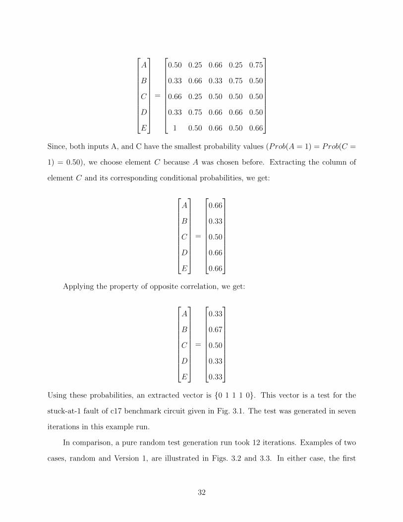
Using these probabilities, an extracted vector is {0 1 1 1 0}. This vector is a test for the

stuck-at-1 fault of c17 benchmark circuit given in Fig. 3.1. The test was generated in seven

iterations in this example run.

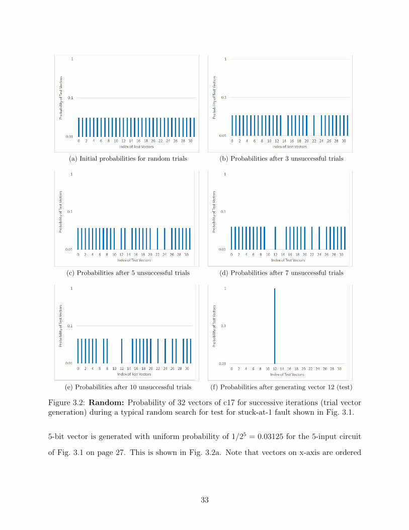
In comparison, a pure random test generation run took 12 iterations. Examples of two

cases, random and Version 1, are illustrated in Figs. 3.2 and 3.3. In either case, the first

32

(a) Initial probabilities for random trials (b) Probabilities after 3 unsuccessful trials

(c) Probabilities after 5 unsuccessful trials (d) Probabilities after 7 unsuccessful trials

(e) Probabilities after 10 unsuccessful trials (f) Probabilities after generating vector 12 (test)

Figure 3.2: Random: Probability of 32 vectors of c17 for successive iterations (trial vectorgeneration) during a typical random search for test for stuck-at-1 fault shown in Fig. 3.1.

5-bit vector is generated with uniform probability of 1/25 = 0.03125 for the 5-input circuit

of Fig. 3.1 on page 27. This is shown in Fig. 3.2a. Note that vectors on x-axis are ordered

33

(a) Initial vector probabilities (b) Vector probabilities after 3 unsuccessful trials

(c) Vector probabilities after 5 unsuccessful trials (d) Vector probabilities after 7th successful trial

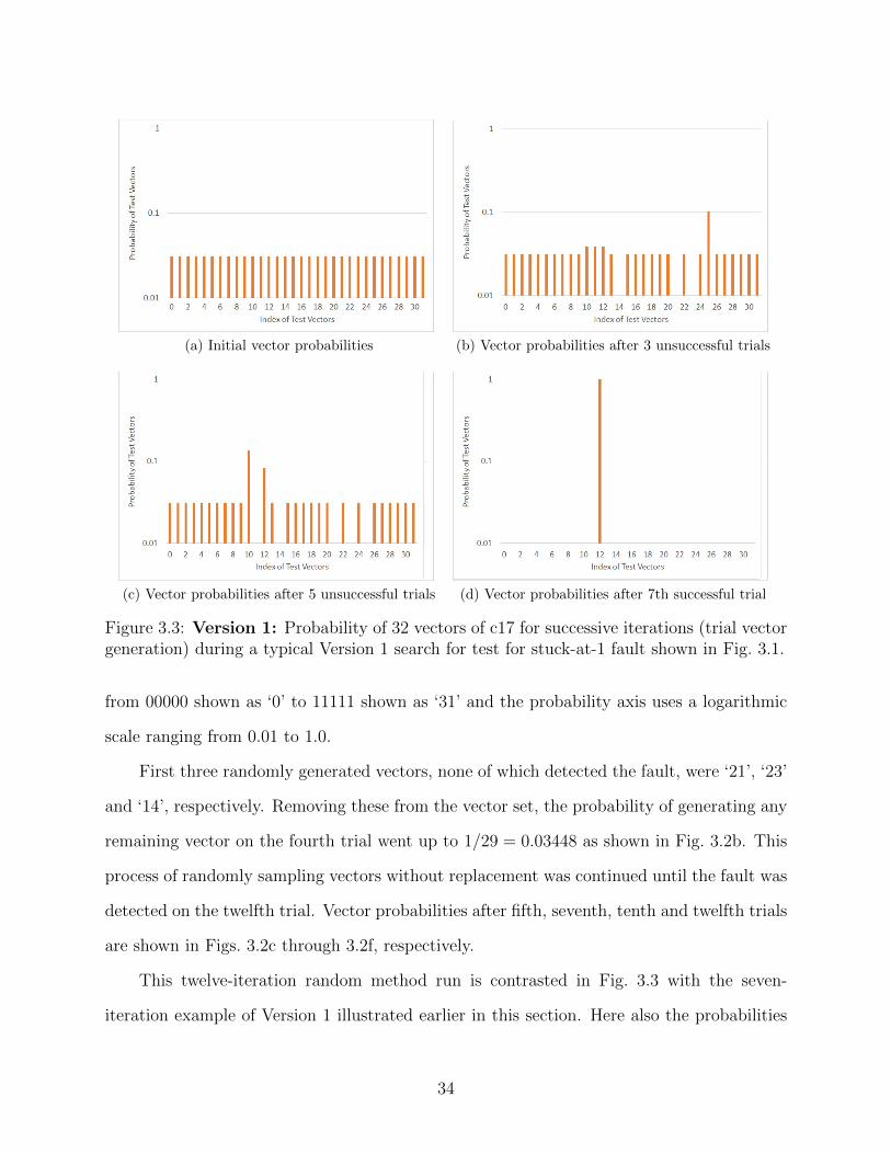
Figure 3.3: Version 1: Probability of 32 vectors of c17 for successive iterations (trial vectorgeneration) during a typical Version 1 search for test for stuck-at-1 fault shown in Fig. 3.1.

from 00000 shown as ‘0’ to 11111 shown as ‘31’ and the probability axis uses a logarithmic

scale ranging from 0.01 to 1.0.

First three randomly generated vectors, none of which detected the fault, were ‘21’, ‘23’

and ‘14’, respectively. Removing these from the vector set, the probability of generating any

remaining vector on the fourth trial went up to 1/29 = 0.03448 as shown in Fig. 3.2b. This

process of randomly sampling vectors without replacement was continued until the fault was

detected on the twelfth trial. Vector probabilities after fifth, seventh, tenth and twelfth trials

are shown in Figs. 3.2c through 3.2f, respectively.

This twelve-iteration random method run is contrasted in Fig. 3.3 with the seven-

iteration example of Version 1 illustrated earlier in this section. Here also the probabilities

34

of unsuccessful vectors drop to zero for subsequent iterations, but the bit correlations and

avoidance of unsuccessful vector characteristics boost probabilities of some vectors at the

cost of others.

The algorithm Version 1 showed some initial promise and example runs demonstrated a

dramatic speed-up over random search for small circuits. However, this algorithm could not

scale up because for a large vector space with just one or very few test vectors, it became

akin to searching for a “needle in a haystack”. By simply trying to avoid the failed vector

properties, the sheer number of failed vectors masked the correct test vector. It became

clear that it was not sufficient merely to avoid all failed vectors, but it is important to

closely examine the failed vectors for their desirable features. Hence, a modification was

made and the next version was developed.

3.2 Version 2

It is colloquially understood that there are a lot more failed test vectors generated as

compared to successful ones when attempting to successfully test a fault (especially a hard-

to-detect fault). Our algorithm deduces the correct test vector by learning the properties of

failed test vectors and avoiding their properties in subsequent iterations. The algorithm’s

search is aided by classifying all the test vectors in the vector space into three broad cate-

gories [85]:

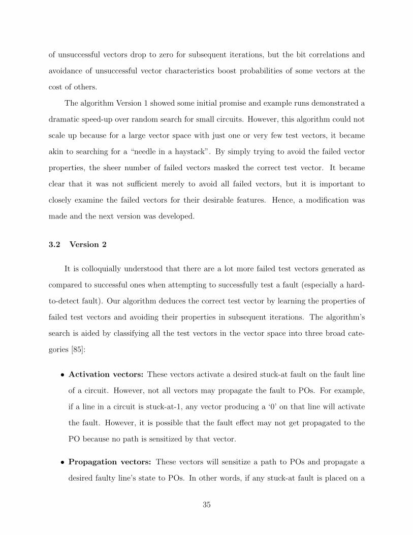
• Activation vectors: These vectors activate a desired stuck-at fault on the fault line

of a circuit. However, not all vectors may propagate the fault to POs. For example,

if a line in a circuit is stuck-at-1, any vector producing a ‘0’ on that line will activate

the fault. However, it is possible that the fault effect may not get propagated to the

PO because no path is sensitized by that vector.

• Propagation vectors: These vectors will sensitize a path to POs and propagate a

desired faulty line’s state to POs. In other words, if any stuck-at fault is placed on a

35

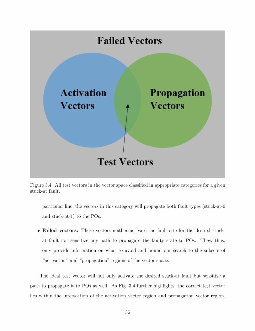
Figure 3.4: All test vectors in the vector space classified in appropriate categories for a givenstuck-at fault.

particular line, the vectors in this category will propagate both fault types (stuck-at-0

and stuck-at-1) to the POs.

• Failed vectors: These vectors neither activate the fault site for the desired stuck-

at fault nor sensitize any path to propagate the faulty state to POs. They, thus,

only provide information on what to avoid and bound our search to the subsets of

“activation” and “propagation” regions of the vector space.

The ideal test vector will not only activate the desired stuck-at fault but sensitize a

path to propagate it to POs as well. As Fig. 3.4 further highlights, the correct test vector

lies within the intersection of the activation vector region and propagation vector region.

36

However, hard-to-detect faults may have only one or two such unique vectors. It is easier

to find vectors that can either activate the fault but do not sensitize a path or, conversely,

sensitize a path but not activate the fault. These vectors have useful information, which can

be used to hone into the correct solution steadily. The failed vectors restrict our search in

the region of “partial desirability” and hence act as a fence so that we do not search outside

of those constraints.

3.2.1 Implementation

The algorithm’s concept outlined in the previous section can be implemented in a variety

of ways or techniques. The proposed implementation utilizes a method of skewing the

independent weighted probabilities of PIs in a manner so that the search moves away from

the failed test vector region. Simply stated, we postulate that if a certain probability weight

at the PI generates a logic value (’1’ or ’0’), which neither activates the fault nor sensitizes

a path to POs, then it is best to invert the probability weight before generating a new value

for that line. This method is repeated till the search enters the region of activation vectors

and/or propagation vectors (colloquially, region of “partial desirability”).

Once the search enters either of these regions, it is in our best interest that the search

does not deviate away from this subset of vector space. From here on now, the weighted

probability of the failed vectors is used to modify the weighted probability of the vectors in

the partial desirability region. These modifications are made in smaller increments in order

to take smaller steps toward the correct test vector. Figure 3.5 on the following page gives a

detailed flowchart of the implementation process of the concept highlighted in the previous

section.

Version 2 showed significant advantage over Version 1 demonstrating the benefit of clas-

sification of failed vectors according to their ability to fault activation, fault propagation, or

doing neither. Encouraged with this result we combined all three characteristics, namely, use

37

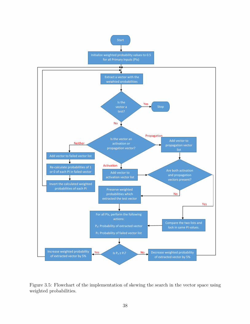
Initialize weighted probability values to 0.5

for all Primary Inputs (PIs)

Extract a vector with the

weighted probabilities

Is the

vector a

test?

Is the vector an

activation or

propagation vector?

Add vector to

propagation vector

list

Add vector to

activation vector list

Are both activation

and propagation

vectors present?

Compare the two lists and

lock in same PI values.

Preserve weighted

probabilities which

extracted the test vector

Start

For all PIs, perform the following

actions:

Pd: Probability of extracted vector

Pf: Probability of failed vector list

Is Pd ≥ Pf? Increase weighted probability

of extracted vector by 5% Decrease weighted probability

of extracted vector by 5%

Add vector to failed vector list

Re-calculate probabilities of 1

or 0 of each PI in failed vector

list

Invert the calculated weighted

probabilities of each PI

Stop

Neither

No

Propagation

Yes

No Yes

Activation

Yes

No

Figure 3.5: Flowchart of the implementation of skewing the search in the vector space usingweighted probabilities.

38

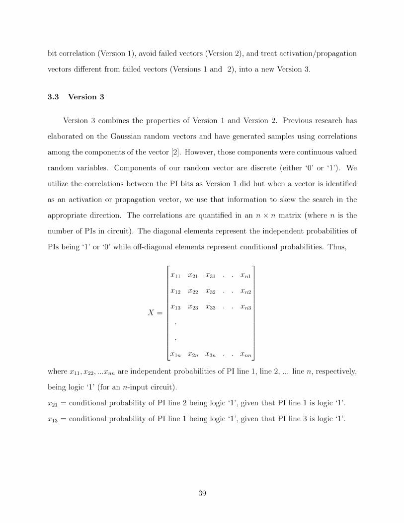
bit correlation (Version 1), avoid failed vectors (Version 2), and treat activation/propagation

vectors different from failed vectors (Versions 1 and 2), into a new Version 3.

3.3 Version 3

Version 3 combines the properties of Version 1 and Version 2. Previous research has

elaborated on the Gaussian random vectors and have generated samples using correlations

among the components of the vector [2]. However, those components were continuous valued

random variables. Components of our random vector are discrete (either ‘0’ or ‘1’). We

utilize the correlations between the PI bits as Version 1 did but when a vector is identified

as an activation or propagation vector, we use that information to skew the search in the

appropriate direction. The correlations are quantified in an n × n matrix (where n is the

number of PIs in circuit). The diagonal elements represent the independent probabilities of

PIs being ‘1’ or ‘0’ while off-diagonal elements represent conditional probabilities. Thus,

X =

x11 x21 x31 . . xn1

x12 x22 x32 . . xn2

x13 x23 x33 . . xn3

.

.

x1n x2n x3n . . xnn

where x11, x22, ...xnn are independent probabilities of PI line 1, line 2, ... line n, respectively,

being logic ‘1’ (for an n-input circuit).

x21 = conditional probability of PI line 2 being logic ‘1’, given that PI line 1 is logic ‘1’.

x13 = conditional probability of PI line 1 being logic ‘1’, given that PI line 3 is logic ‘1’.

39

3.3.1 Algorithm Steps

This subsection describes in detail how the algorithm has been implemented and the

steps or iterations needed to perform a successful search of test vectors:

i. Initialize all elements of the n× n matrix with probability value of 0.50. The diagonal

elements represent the independent probabilities of the PI bits while the off-diagonal

elements are the conditional probabilities.

ii. Choose a PI and extract a ‘1’ or ‘0’, given the probability (diagonal element in the

matrix) for that PI.

iii. Given the previous PI’s bit value as ‘0’ or ‘1’, recalculate the conditional probability

matrix with respect to the previously extracted bit. Now derive a bit value for the

next PI.

iv. Given the bit values of the first two PIs, recalculate the conditional probability matrix

and extract a bit value for the third PI.

v. Keep extracting bit values one by one for all PIs using the conditional probability with

respect to the previously extracted PIs, until all n bits are extracted.

vi. Use the newly extracted test vector to simulate the stuck-at fault. If the vector is a

test, stop the procedure, else go to the next step.

vii. If the vector is not a test, check simulation data to determine whether it is an activation

or a propagation vector. If the vector is either of those, add it to the appropriate

activation or propagation vector list and preserve the probability matrix that generated

this vector. Repeat from step ii until a test is found.

viii. If the extracted vector is neither an activation nor a propagation vector, add it to the

failed test vector list. Recalculate the probability matrix from the failed test vectors

and repeat from step ii until a test is found.

40

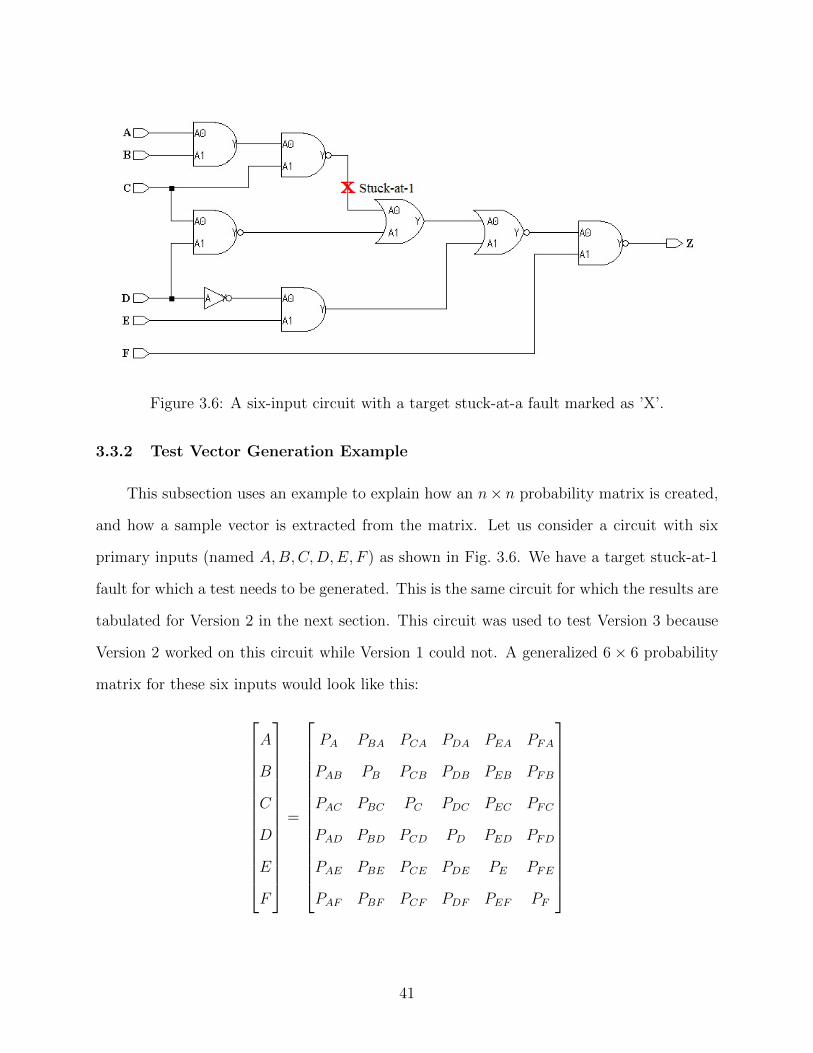
Figure 3.6: A six-input circuit with a target stuck-at-a fault marked as ’X’.

3.3.2 Test Vector Generation Example

This subsection uses an example to explain how an n× n probability matrix is created,

and how a sample vector is extracted from the matrix. Let us consider a circuit with six

primary inputs (named A,B,C,D,E, F ) as shown in Fig. 3.6. We have a target stuck-at-1

fault for which a test needs to be generated. This is the same circuit for which the results are

tabulated for Version 2 in the next section. This circuit was used to test Version 3 because

Version 2 worked on this circuit while Version 1 could not. A generalized 6× 6 probability

matrix for these six inputs would look like this:

A

B

C

D

E

F

=

PA PBA PCA PDA PEA PFA

PAB PB PCB PDB PEB PFB

PAC PBC PC PDC PEC PFC

PAD PBD PCD PD PED PFD

PAE PBE PCE PDE PE PFE

PAF PBF PCF PDF PEF PF

41

where the diagonals represent the independent probabilities of each input while the off-

diagonal elements represent the conditional probabilities of an input with respect to another

input.

Let us assume the following 10 vectors have all failed to detect the target stuck-at fault:

A B C D E F

0 0 1 0 1 0

1 1 0 1 0 1

0 1 0 0 1 1

1 0 0 1 1 1

1 0 0 0 0 0

1 0 0 0 0 1

0 1 0 0 1 1

0 0 0 0 0 0

1 0 0 0 1 0

1 1 1 1 0 0

Using these vectors, the probability matrix would look like this:

A

B

C

D

E

F

=

0.60 0.33 0.17 0.50 0.33 0.50

0.50 0.40 0.25 0.50 0.50 0.75

0.50 0.50 0.20 0.50 0.50 0

1 0.67 0.33 0.30 0.33 0.67

0.40 0.40 0.20 0.20 0.50 0.40

0.75 0.50 0 0.50 0.50 0.40

From this matrix, Prob(A = 1) = 0.60, which means the failed vectors have more ‘1’s than

42

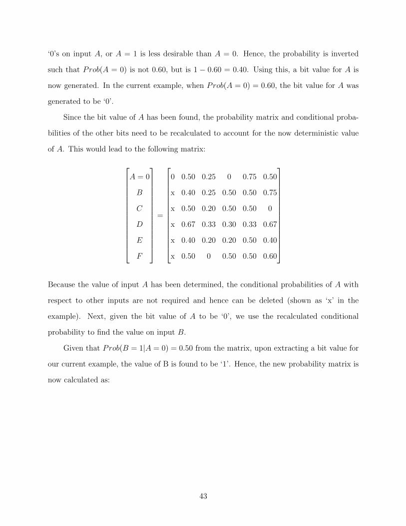
‘0’s on input A, or A = 1 is less desirable than A = 0. Hence, the probability is inverted

such that Prob(A = 0) is not 0.60, but is 1 − 0.60 = 0.40. Using this, a bit value for A is

now generated. In the current example, when Prob(A = 0) = 0.60, the bit value for A was

generated to be ‘0’.

Since the bit value of A has been found, the probability matrix and conditional proba-

bilities of the other bits need to be recalculated to account for the now deterministic value

of A. This would lead to the following matrix:

A = 0

B

C

D

E

F

=

0 0.50 0.25 0 0.75 0.50

x 0.40 0.25 0.50 0.50 0.75

x 0.50 0.20 0.50 0.50 0

x 0.67 0.33 0.30 0.33 0.67

x 0.40 0.20 0.20 0.50 0.40

x 0.50 0 0.50 0.50 0.60

Because the value of input A has been determined, the conditional probabilities of A with

respect to other inputs are not required and hence can be deleted (shown as ‘x’ in the

example). Next, given the bit value of A to be ‘0’, we use the recalculated conditional

probability to find the value on input B.

Given that Prob(B = 1|A = 0) = 0.50 from the matrix, upon extracting a bit value for

our current example, the value of B is found to be ‘1’. Hence, the new probability matrix is

now calculated as:

43

A = 0

B = 1

C

D

E

F

=

0 x 0.25 0 0.75 0.50

x 1 0.25 0.50 0.50 0.75

x x 0.20 0.50 0.50 0

x x 0.33 0.30 0.33 0.67

x x 0.20 0.20 0.50 0.40

x x 0 0.50 0.50 0.60

For values of A and B to be ‘0’ and ‘1’, respectively, we use the conditional probabilities of

each bit on C to find a new normalized bit probability for C. In other words,

Prob(C = 1|A = 0) = 0.25, and Prob(C = 1|B = 1) = 0.25.

Therefore, Prob(C = 1|A = 0, B = 1) = (0.25 + 0.25)/2 = 0.25.

Since, all previous vectors are failed vectors, we want to find new vectors with opposite

correlations. This implies that we generate a bit value from Prob(C = 0|A = 0, B = 1) =

0.25. In our example, this resulted in a value ‘0’ for input C. The new recalculated probability

matrix is as follows:

A = 0

B = 1

C = 0

D

E

F

=

0 x x 0 0.75 0.50

x 1 x 0.50 0.50 0.75

x x 0 0.25 0.50 0.50

x x x 0.30 0.33 0.67

x x x 0.20 0.50 0.40

x x x 0.50 0.50 0.60

Given bit values A = 0, B = 1 and C = 0, we find the conditional probability for D. In

44

other words,

Prob(D = 1|A = 0) = 0, Prob(D = 1|B = 1) = 0.50, and Prob(D = 1|C = 0) = 0.25.

Therefore, Prob(D = 1|A = 0, B = 1, C = 0) = (0 + 0.50 + 0.25)/3 = 0.25.

Since, we want opposite correlations, we will generate a bit value for D using Prob(D =

0|A = 0, B = 1, C = 0) = 0.25. In this example, this resulted in a the value ‘1’ for input D.

The new recalculated probability matrix is as follows:

A = 0

B = 1

C = 0

D = 1

E

F

=

0 x x x 0.75 0.50

x 1 x x 0.50 0.75

x x 0 x 0.50 0.50

x x x 1 0.33 0.67

x x x x 0.50 0.40

x x x x 0.50 0.60

Now, A = 0, B = 1, C = 0 and D = 1. Using their influence on input E and normalizing

the conditional probability, we get

Prob(E = 1|A = 0) = 0.75, Prob(E = 1|B = 1) = 0.50, Prob(E = 1|C = 0) = 0.38,

and Prob(E = 1|D = 1) = 0.33.

Therefore, P (E = 1|A = 0, B = 1, C = 0, D = 1) = (0.75+0.50+0.38+0.33)/4 = 0.49.

As before, utilizing the need for opposite correlation, P (E = 0|A = 0, B = 1, C =

0, D = 1) = 0.49, resulting in a bit value ‘0’ on input E for our example. The recalculated

probability matrix is:

45

A = 0

B = 1

C = 0

D = 1

E = 0

F

=

0 x x x x 0.50

x 1 x x x 0.75

x x 0 x x 0.50

x x x 1 x 0.67

x x x x 0 0.40

x x x x x 0.40

For the last input F , we already have A = 0, B = 1, C = 0, D = 1 and E = 0. The

normalized conditional probability of F is obtained as follows:

Prob(F = 1|A = 0) = 0.50,

Prob(F = 1|B = 1) = 0.75,

Prob(F = 1|C = 0) = 0.50,

Prob(F = 1|D = 1) = 0.67, and

Prob(F = 1|E = 0) = 0.40.

Therefore, Prob(F = 1|A = 0, B = 1, C = 0, D = 1, E = 0) = (0.50 + 0.75 + 0.50 +

0.67 + 0.40)/5 = 0.56.

Utilizing the need for opposite correlation, Prob(F = 0|A = 0, B = 1, C = 0, D =

1, E = 0) = 0.56 resulting in a bit ‘0’ on input F for our example. Hence, the complete

sample vector is {0 1 0 1 0 0}. This will be used in a fault simulator to determine if the

targeted stuck-at-1 (see Fig. 3.6 on page 41)fault was detected. If the vector is not a test, it

will be added to the failed vector list, and a new vector will be generated using the procedure

described above.

46

Chapter 4

Simulation Setup and Tools

The benchmark circuits used for simulations were register-transfer level (RTL) models

written in Verilog. These models are combinational logic circuits gathered from various

online resources such as EPFL combinational benchmark suite [6] and Logic Synthesis and

Optimization Benchmarks (LGSynth’91) [89].

The LGSynth’91 benchmark circuit suite was primarily created for logic synthesis and

optimization and form a continuation of LGSynth’89 benchmark suite. This collection of

sequential and combinational logic circuits also contains finite state machines (FSM) [89].

The EPFL combinational benchmark suite was introduced with an aim of defining a new

comparative standard for logic optimization and synthesis. It consists of 23 combinational

circuits designed to challenge modern logic optimization tools. The benchmark suite is

further divided into arithmetic and random/control circuits [6].

There are 10 types of arithmetic benchmark circuits, like square-root, hypotenuse, di-

visor, multiplier, etc. They are obtained by an automated mapping of arithmetic com-

putational algorithms onto basic logic gates. The arithmetic benchmarks come in different

bit-widths to provide diversity in the implementation complexity. The set of random/control

benchmarks in the EPFL suite consists of various types of controllers, arbiters, routers, con-

verters, decoders, voters and random functions. It contains 10 circuits mapped into simple

gates from behavioral descriptions.

The faults for each benchmark circuit were chosen such that ideally only one test could

detect the fault. For example, for the 11-input combinational logic circuit int2float converter,

there is a stuck-at-1 fault that has only one test (10110011010). However, this fault has 233

47

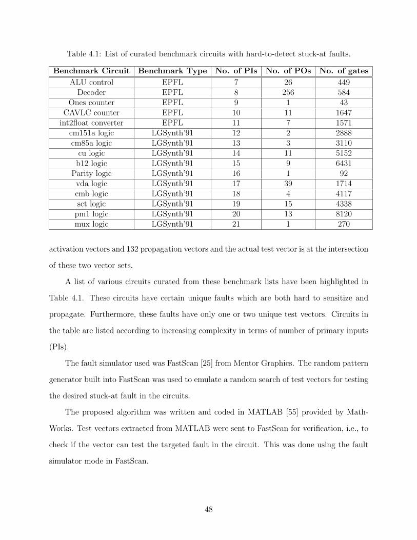
Table 4.1: List of curated benchmark circuits with hard-to-detect stuck-at faults.

Benchmark Circuit Benchmark Type No. of PIs No. of POs No. of gates

ALU control EPFL 7 26 449Decoder EPFL 8 256 584

Ones counter EPFL 9 1 43CAVLC counter EPFL 10 11 1647

int2float converter EPFL 11 7 1571cm151a logic LGSynth’91 12 2 2888cm85a logic LGSynth’91 13 3 3110

cu logic LGSynth’91 14 11 5152b12 logic LGSynth’91 15 9 6431

Parity logic LGSynth’91 16 1 92vda logic LGSynth’91 17 39 1714cmb logic LGSynth’91 18 4 4117sct logic LGSynth’91 19 15 4338

pm1 logic LGSynth’91 20 13 8120mux logic LGSynth’91 21 1 270

activation vectors and 132 propagation vectors and the actual test vector is at the intersection

of these two vector sets.

A list of various circuits curated from these benchmark lists have been highlighted in

Table 4.1. These circuits have certain unique faults which are both hard to sensitize and

propagate. Furthermore, these faults have only one or two unique test vectors. Circuits in

the table are listed according to increasing complexity in terms of number of primary inputs

(PIs).

The fault simulator used was FastScan [25] from Mentor Graphics. The random pattern

generator built into FastScan was used to emulate a random search of test vectors for testing

the desired stuck-at fault in the circuits.

The proposed algorithm was written and coded in MATLAB [55] provided by Math-

Works. Test vectors extracted from MATLAB were sent to FastScan for verification, i.e., to

check if the vector can test the targeted fault in the circuit. This was done using the fault

simulator mode in FastScan.

48

Chapter 5

Results and Discussion

5.1 Version 1 Algorithm Results

Initial results of the Version 1 of our algorithm are for finding a test for a single stuck-at

fault in a 10-input AND gate. The target fault was a stuck-at-1 fault on a primary input

of the gate. This was primarily done to establish the proof of concept of the algorithm and

get a feel of the algorithm’s working by following the mathematics behind it. The algorithm

was also compared with a pure random test generator and a weighted random test generator

based on maximum output entropy [3].

The following figures highlight our results in a graphical manner. Figure 5.1 on the next

page shows the number of iterations needed to find a test for a stuck-at-1 fault in a given

primary input of a 10-input AND gate using our Version 1 algorithm. The test generation

was repeated 100 times and the figure shows the number of times certain number of iterations

was needed to obtain a test. On average the number of iterations was 10.

Figure 5.2 on the following page shows the number of cases (out of 100) versus number of

iterations used to find the test using the entropy based weighted random generator described

by Agrawal [3]. On average, here 25 iterations were needed. Figure 5.3 on page 51 shows

similar results for a pure random test generator for which the average iterations are 512,

which is half the size of the input vector space.

Version 1 was applied to c17 benchmark circuit. This circuit has no hard-to-detect

stuck-at faults. In fact, six test vectors can detect all possible stuck-at faults. Hence, the

Version 1 algorithm was used to find tests for two stuck-at faults, which have the smallest

number of tests. These faults are shown in Fig. 5.4. Table 5.1 compares the algorithm

49

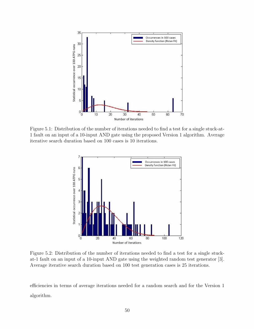
Figure 5.1: Distribution of the number of iterations needed to find a test for a single stuck-at-1 fault on an input of a 10-input AND gate using the proposed Version 1 algorithm. Averageiterative search duration based on 100 cases is 10 iterations.

Figure 5.2: Distribution of the number of iterations needed to find a test for a single stuck-at-1 fault on an input of a 10-input AND gate using the weighted random test generator [3].Average iterative search duration based on 100 test generation cases is 25 iterations.

efficiencies in terms of average iterations needed for a random search and for the Version 1

algorithm.

50

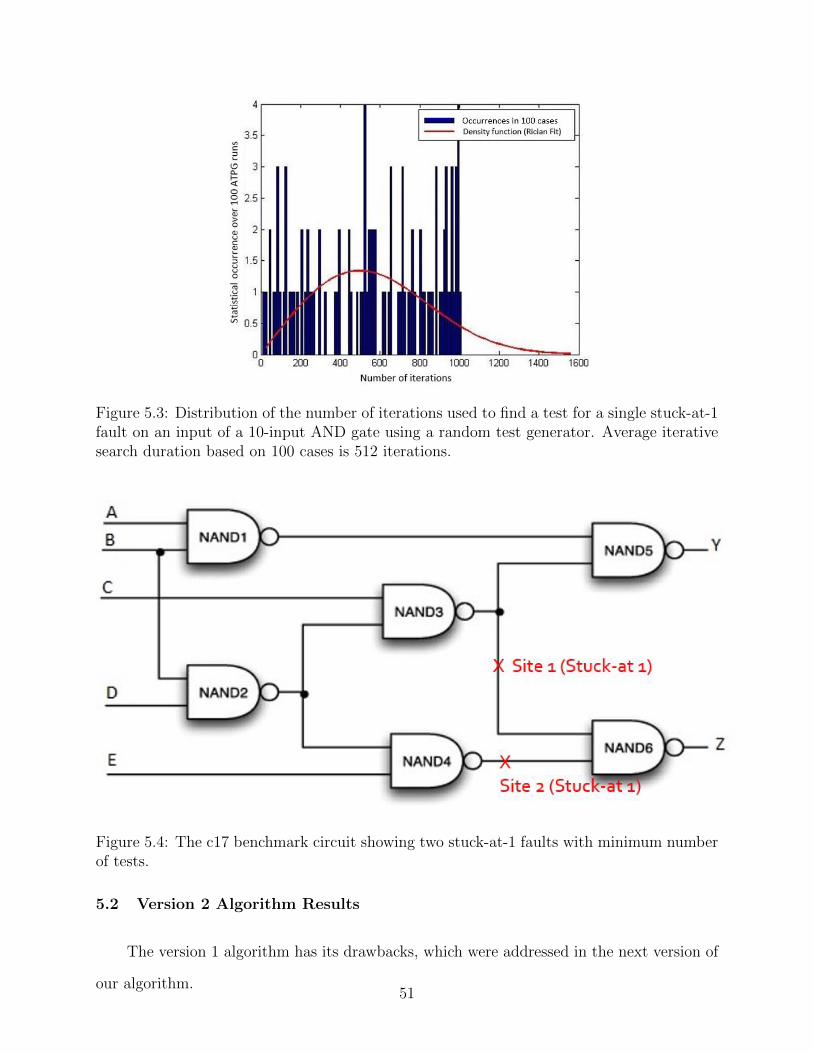
Figure 5.3: Distribution of the number of iterations used to find a test for a single stuck-at-1fault on an input of a 10-input AND gate using a random test generator. Average iterativesearch duration based on 100 cases is 512 iterations.

Figure 5.4: The c17 benchmark circuit showing two stuck-at-1 faults with minimum numberof tests.


The version 1 algorithm has its drawbacks, which were addressed in the next version of

our algorithm.51

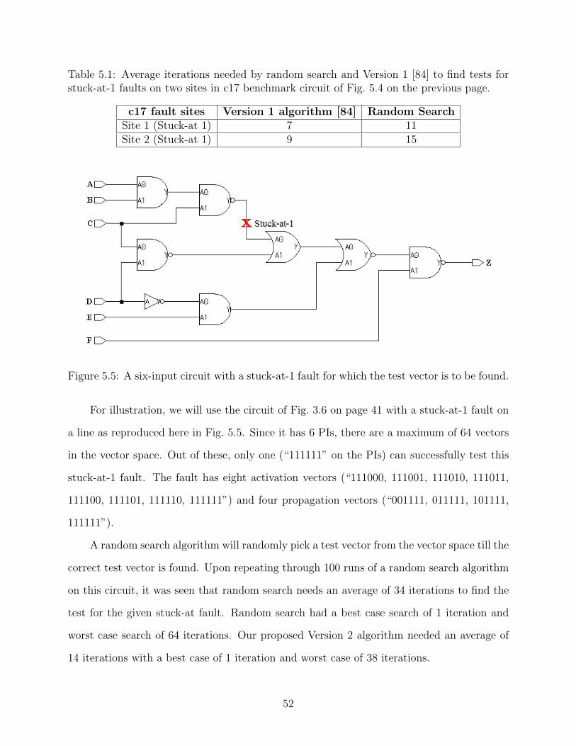
Table 5.1: Average iterations needed by random search and Version 1 [84] to find tests forstuck-at-1 faults on two sites in c17 benchmark circuit of Fig. 5.4 on the previous page.

c17 fault sites Version 1 algorithm [84] Random SearchSite 1 (Stuck-at 1) 7 11Site 2 (Stuck-at 1) 9 15

Figure 5.5: A six-input circuit with a stuck-at-1 fault for which the test vector is to be found.

For illustration, we will use the circuit of Fig. 3.6 on page 41 with a stuck-at-1 fault on

a line as reproduced here in Fig. 5.5. Since it has 6 PIs, there are a maximum of 64 vectors

in the vector space. Out of these, only one (“111111” on the PIs) can successfully test this

stuck-at-1 fault. The fault has eight activation vectors (“111000, 111001, 111010, 111011,

111100, 111101, 111110, 111111”) and four propagation vectors (“001111, 011111, 101111,

111111”).

A random search algorithm will randomly pick a test vector from the vector space till the

correct test vector is found. Upon repeating through 100 runs of a random search algorithm

on this circuit, it was seen that random search needs an average of 34 iterations to find the

test for the given stuck-at fault. Random search had a best case search of 1 iteration and

worst case search of 64 iterations. Our proposed Version 2 algorithm needed an average of

14 iterations with a best case of 1 iteration and worst case of 38 iterations.

52

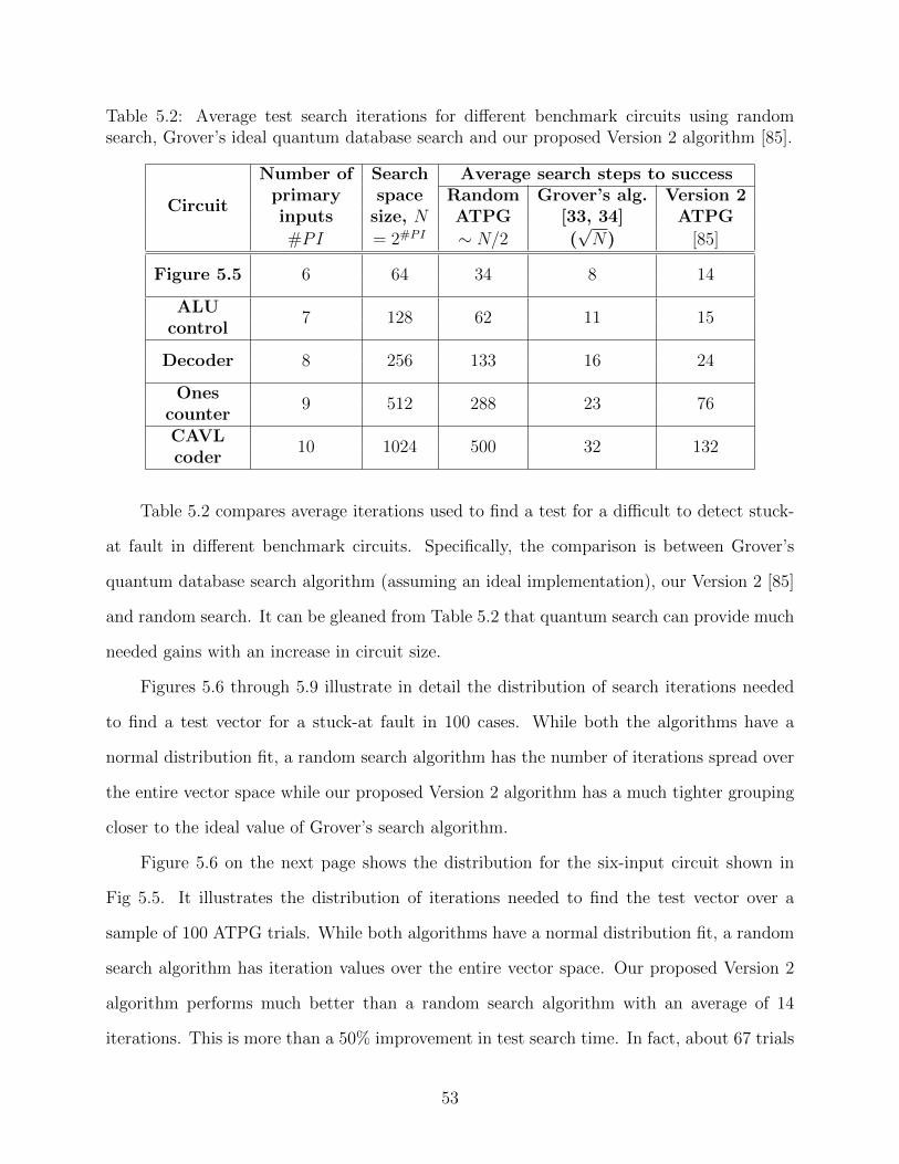
Table 5.2: Average test search iterations for different benchmark circuits using randomsearch, Grover’s ideal quantum database search and our proposed Version 2 algorithm [85].

Circuit

Number of Search Average search steps to successprimary space Random Grover’s alg. Version 2inputs size, N ATPG [33, 34] ATPG

#PI = 2#PI ∼ N/2 (√N) [85]

Figure 5.5 6 64 34 8 14

ALU7 128 62 11 15

control

Decoder 8 256 133 16 24

Ones9 512 288 23 76

counterCAVL

10 1024 500 32 132coder

Table 5.2 compares average iterations used to find a test for a difficult to detect stuck-

at fault in different benchmark circuits. Specifically, the comparison is between Grover’s

quantum database search algorithm (assuming an ideal implementation), our Version 2 [85]

and random search. It can be gleaned from Table 5.2 that quantum search can provide much

needed gains with an increase in circuit size.

Figures 5.6 through 5.9 illustrate in detail the distribution of search iterations needed

to find a test vector for a stuck-at fault in 100 cases. While both the algorithms have a

normal distribution fit, a random search algorithm has the number of iterations spread over

the entire vector space while our proposed Version 2 algorithm has a much tighter grouping

closer to the ideal value of Grover’s search algorithm.

Figure 5.6 on the next page shows the distribution for the six-input circuit shown in

Fig 5.5. It illustrates the distribution of iterations needed to find the test vector over a

sample of 100 ATPG trials. While both algorithms have a normal distribution fit, a random

search algorithm has iteration values over the entire vector space. Our proposed Version 2

algorithm performs much better than a random search algorithm with an average of 14

iterations. This is more than a 50% improvement in test search time. In fact, about 67 trials

53

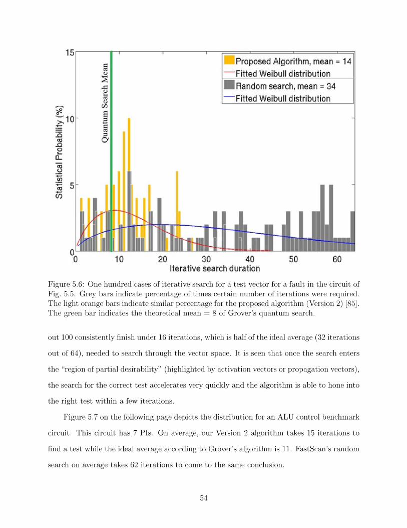
Figure 5.6: One hundred cases of iterative search for a test vector for a fault in the circuit ofFig. 5.5. Grey bars indicate percentage of times certain number of iterations were required.The light orange bars indicate similar percentage for the proposed algorithm (Version 2) [85].The green bar indicates the theoretical mean = 8 of Grover’s quantum search.

out 100 consistently finish under 16 iterations, which is half of the ideal average (32 iterations

out of 64), needed to search through the vector space. It is seen that once the search enters

the “region of partial desirability” (highlighted by activation vectors or propagation vectors),

the search for the correct test accelerates very quickly and the algorithm is able to hone into

the right test within a few iterations.

Figure 5.7 on the following page depicts the distribution for an ALU control benchmark

circuit. This circuit has 7 PIs. On average, our Version 2 algorithm takes 15 iterations to

find a test while the ideal average according to Grover’s algorithm is 11. FastScan’s random

search on average takes 62 iterations to come to the same conclusion.

54

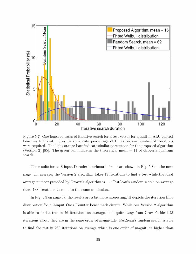
Figure 5.7: One hundred cases of iterative search for a test vector for a fault in ALU controlbenchmark circuit. Grey bars indicate percentage of times certain number of iterationswere required. The light orange bars indicate similar percentage for the proposed algorithm(Version 2) [85]. The green bar indicates the theoretical mean = 11 of Grover’s quantumsearch.

The results for an 8-input Decoder benchmark circuit are shown in Fig. 5.8 on the next

page. On average, the Version 2 algorithm takes 15 iterations to find a test while the ideal

average number provided by Grover’s algorithm is 11. FastScan’s random search on average

takes 133 iterations to come to the same conclusion.

In Fig. 5.9 on page 57, the results are a bit more interesting. It depicts the iteration time

distribution for a 9-input Ones Counter benchmark circuit. While our Version 2 algorithm

is able to find a test in 76 iterations on average, it is quite away from Grover’s ideal 23

iterations albeit they are in the same order of magnitude. FastScan’s random search is able

to find the test in 288 iterations on average which is one order of magnitude higher than

55

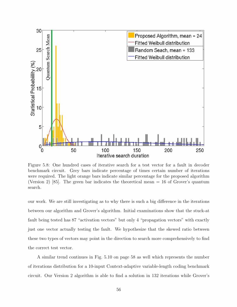
Figure 5.8: One hundred cases of iterative search for a test vector for a fault in decoderbenchmark circuit. Grey bars indicate percentage of times certain number of iterationswere required. The light orange bars indicate similar percentage for the proposed algorithm(Version 2) [85]. The green bar indicates the theoretical mean = 16 of Grover’s quantumsearch.

our work. We are still investigating as to why there is such a big difference in the iterations

between our algorithm and Grover’s algorithm. Initial examinations show that the stuck-at

fault being tested has 87 “activation vectors” but only 4 “propagation vectors” with exactly

just one vector actually testing the fault. We hypothesize that the skewed ratio between

these two types of vectors may point in the direction to search more comprehensively to find

the correct test vector.

A similar trend continues in Fig. 5.10 on page 58 as well which represents the number

of iterations distribution for a 10-input Context-adaptive variable-length coding benchmark

circuit. Our Version 2 algorithm is able to find a solution in 132 iterations while Grover’s

56

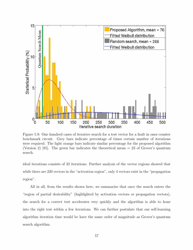
Figure 5.9: One hundred cases of iterative search for a test vector for a fault in ones counterbenchmark circuit. Grey bars indicate percentage of times certain number of iterationswere required. The light orange bars indicate similar percentage for the proposed algorithm(Version 2) [85]. The green bar indicates the theoretical mean = 23 of Grover’s quantumsearch.

ideal iterations consists of 32 iterations. Further analysis of the vector regions showed that

while there are 220 vectors in the “activation region”, only 4 vectors exist in the “propagation

region”.

All in all, from the results shown here, we summarize that once the search enters the

“region of partial desirability” (highlighted by activation vectors or propagation vectors),

the search for a correct test accelerates very quickly and the algorithm is able to hone

into the right test within a few iterations. We can further postulate that our self-learning

algorithm iteration time would be have the same order of magnitude as Grover’s quantum

search algorithm.

57

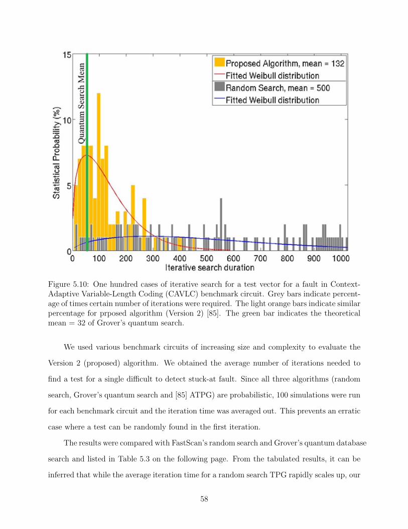
Figure 5.10: One hundred cases of iterative search for a test vector for a fault in Context-Adaptive Variable-Length Coding (CAVLC) benchmark circuit. Grey bars indicate percent-age of times certain number of iterations were required. The light orange bars indicate similarpercentage for prposed algorithm (Version 2) [85]. The green bar indicates the theoreticalmean = 32 of Grover’s quantum search.

We used various benchmark circuits of increasing size and complexity to evaluate the

Version 2 (proposed) algorithm. We obtained the average number of iterations needed to

find a test for a single difficult to detect stuck-at fault. Since all three algorithms (random

search, Grover’s quantum search and [85] ATPG) are probabilistic, 100 simulations were run

for each benchmark circuit and the iteration time was averaged out. This prevents an erratic

case where a test can be randomly found in the first iteration.

The results were compared with FastScan’s random search and Grover’s quantum database

search and listed in Table 5.3 on the following page. From the tabulated results, it can be

inferred that while the average iteration time for a random search TPG rapidly scales up, our

58

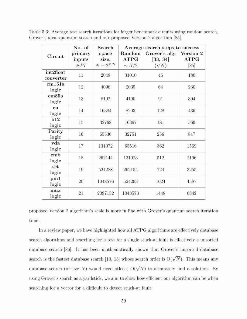
Table 5.3: Average test search iterations for larger benchmark circuits using random search,Grover’s ideal quantum search and our proposed Version 2 algorithm [85].

Circuit

No. of Search Average search steps to successprimary space Random Grover’s alg. Version 2inputs size, ATPG [33, 34] ATPG

#PI N = 2#PI ∼ N/2 (√N) [85]

int2float11 2048 31010 46 180

convertercm151a

12 4096 2035 64 230logic

cm85a13 8192 4100 91 304

logiccu

14 16384 8203 128 436logicb12

15 32768 16367 181 569logic

Parity16 65536 32751 256 847

logicvda

17 131072 65516 362 1569logiccmb

18 262144 131023 512 2196logicsct

19 524288 262154 724 3255logicpm1

20 1048576 524293 1024 4587logicmux

21 2097152 1048573 1448 6842logic

proposed Version 2 algorithm’s scale is more in line with Grover’s quantum search iteration

time.

In a review paper, we have highlighted how all ATPG algorithms are effectively database

search algorithms and searching for a test for a single stuck-at fault is effectively a unsorted

database search [86]. It has been mathematically shown that Grover’s unsorted database

search is the fastest database search [10, 13] whose search order is O(√N). This means any

database search (of size N) would need atleast O(√N) to accurately find a solution. By

using Grover’s search as a yardstick, we aim to show how efficient our algorithm can be when

searching for a vector for a difficult to detect stuck-at fault.

59

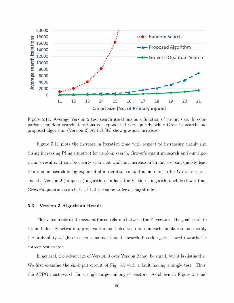
Figure 5.11: Average Version 2 test search iterations as a function of circuit size. In com-parison, random search iterations go exponential very quickly while Grover’s search andproposed algorithm (Version 2) ATPG [85] show gradual increases.

Figure 5.11 plots the increase in iteration time with respect to increasing circuit size

(using increasing PI as a metric) for random search, Grover’s quantum search and our algo-

rithm’s results. It can be clearly seen that while an increase in circuit size can quickly lead

to a random search being exponential in iteration time, it is more linear for Grover’s search

and the Version 2 (proposed) algorithm. In fact, the Version 2 algorithm, while slower than

Grover’s quantum search, is still of the same order of magnitude.


This version takes into account the correlation between the PI vectors. The goal is still to

try and identify activation, propagation and failed vectors from each simulation and modify

the probability weights in such a manner that the search direction gets skewed towards the

correct test vector.

In general, the advantage of Version 3 over Version 2 may be small, but it is distinctive.

We first examine the six-input circuit of Fig. 5.5 with a fault having a single test. Thus,

the ATPG must search for a single target among 64 vectors. As shown in Figure 5.6 and

60

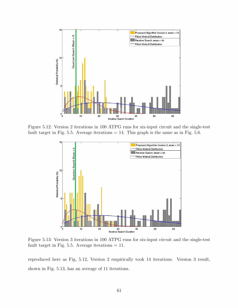
Figure 5.12: Version 2 iterations in 100 ATPG runs for six-input circuit and the single-testfault target in Fig. 5.5. Average iterations = 14. This graph is the same as in Fig. 5.6.

Figure 5.13: Version 3 iterations in 100 ATPG runs for six-input circuit and the single-testfault target in Fig. 5.5. Average iterations = 11.

reproduced here as Fig, 5.12, Version 2 empirically took 14 iterations. Version 3 result,

shown in Fig. 5.13, has an average of 11 iterations.

61

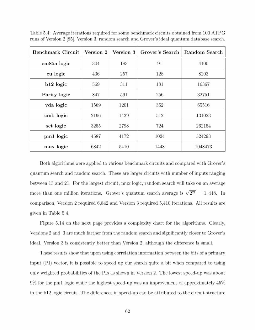
Table 5.4: Average iterations required for some benchmark circuits obtained from 100 ATPGruns of Version 2 [85], Version 3, random search and Grover’s ideal quantum database search.

Benchmark Circuit Version 2 Version 3 Grover’s Search Random Search

cm85a logic 304 183 91 4100

cu logic 436 257 128 8203

b12 logic 569 311 181 16367

Parity logic 847 591 256 32751

vda logic 1569 1201 362 65516

cmb logic 2196 1429 512 131023

sct logic 3255 2798 724 262154

pm1 logic 4587 4172 1024 524293

mux logic 6842 5410 1448 1048473

Both algorithms were applied to various benchmark circuits and compared with Grover’s

quantum search and random search. These are larger circuits with number of inputs ranging

between 13 and 21. For the largest circuit, mux logic, random search will take on an average

more than one million iterations. Grover’s quantum search average is√

221 = 1, 448. In

comparison, Version 2 required 6,842 and Version 3 required 5,410 iterations. All results are

given in Table 5.4.

Figure 5.14 on the next page provides a complexity chart for the algorithms. Clearly,

Versions 2 and 3 are much farther from the random search and significantly closer to Grover’s

ideal. Version 3 is consistently better than Version 2, although the difference is small.

These results show that upon using correlation information between the bits of a primary

input (PI) vector, it is possible to speed up our search quite a bit when compared to using

only weighted probabilities of the PIs as shown in Version 2. The lowest speed-up was about

9% for the pm1 logic while the highest speed-up was an improvement of approximately 45%

in the b12 logic circuit. The differences in speed-up can be attributed to the circuit structure

62

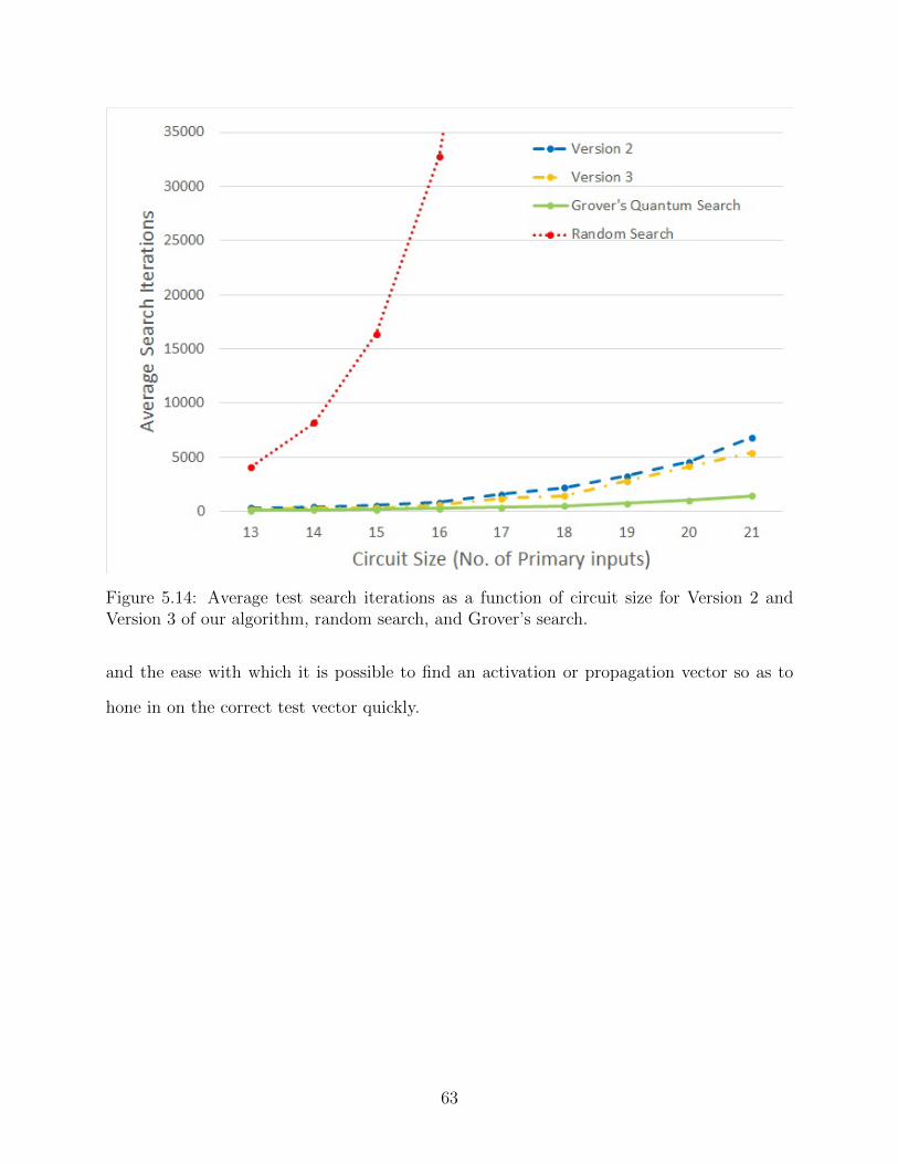
Figure 5.14: Average test search iterations as a function of circuit size for Version 2 andVersion 3 of our algorithm, random search, and Grover’s search.

and the ease with which it is possible to find an activation or propagation vector so as to

hone in on the correct test vector quickly.

63

Chapter 6

Conclusion

We believe we have opened a new chapter in the area of VLSI Testing. It is seen that

failure evasion is a good technique for finding test vectors for hard to difficult stuck-at faults.

It has also been shown that utilizing the correlation between the test vectors can be very

effective in searching for the correct test vector for a stuck-at fault. This can lead to other

avenues of future research. Firstly, our work only elaborates on one possible technique on the

utilization of correlations among test vectors. Other mathematical techniques like steepest

descent [37], where one takes proportional steps from the current point to the desired solution,

or conjugate gradient descent [79] which can solve unconstrained optimization problems can

also be used.

This work focuses mainly on the hard-to-detect stuck-at fault and the core feature behind

this work is “Given a fault, find a test.” The work can be easily expanded to encompass all

stuck-at faults and to find vectors which test those faults. Another future work would be to

integrate this work with other known testing algorithms. Different testing algorithms have

different strengths and target different types of faults. By integrating these together, we can

create a “Grand Unified ATPG” which can target any type of fault. Basically, since the

technique is based on fault simulation, tests can be generated for any fault model provided

it can be simulated.

Finally, the question of using Grover’s quantum algorithm of database search for search-

ing through the database of unordered test vectors is still unanswered. This work only points

in the direction of where future VLSI testing research can head towards and a practical im-

plementation of a quantum search still needs to be found. It may be possible that until a

64

quantum computer can actually be conceived, the question of creating a testing algorithm

which can utilize a quantum speed-up will still remain open.

This dissertation attempts to put to rest the stagnation claims about the VLSI Testing

field. The background research shows how ATPG algorithms have evolved in the past 50

years. With the dramatic rise in research in the area of quantum computing, it is only

natural to use those ideas to break the VLSI Testing area out of its plateau.

By showing how the testing problem can be redefined as a database search problem

and how various ATPG algorithms are essentially formulations of classic database search

algorithms, our work encourages the use of Grover’s algorithm for database search as the

template for creating new APTG algorithms. A literature survey shows how little research

has been done in this field, and the results of the few forays into the application of Grover’s

algorithm have shown startling promise and dramatic test time improvement.

Our results should encourage other researchers to develop other techniques and method-

ologies to effectively utilize failures as a guide to improve search time in test vector gener-

ation. Researchers are only limited by their imagination in trying to find solutions for NP

hard problems. The authors encourage the pushing of current boundaries and the bold ex-

ploration of new ideas. Until it is proven for certain that a given solution is the most optimal,

there is always hope that paradigms will continue to shift and it is immature to claim the

maturity of a research field.

65

Bibliography

[1] P. Agrawal and V. D. Agrawal, “Probabilistic Analysis of Random Test Generation

Method for Irredundant Combinational Logic Networks,” IEEE Trans. on Computers,

vol. C-24, no. 7, pp. 691–695, July 1975.

[2] V. D. Agrawal, Mutual Coupling in Phased Arrays of Randomly Spaced Antennas. PhD

thesis, University of Illinois at Urbana-Champaign, Urbana, IL, Jan. 1971.

[3] V. D. Agrawal, “An Information Theoretic Approach to Digital Fault Testing,” IEEE

Trans. Computers, vol. 30, no. 8, pp. 582–587, 1981.

[4] V. D. Agrawal and P. Agrawal, “An Automatic Test Generation System for ILLIAC IV

Logic Boards,” IEEE Trans. on Computers, vol. C-21, pp. 1015–1017, Sept. 1972.

[5] S. B. Akers, “Universal Test Sets for Logic Networks,” in IEEE Conference Record of

13th Annual Symposium on Switching and Automata Theory, 1972, pp. 177–184.

[6] L. Amaru, P.-E. Gaillardon, and G. De Micheli, “The EPFL Combinational Benchmark

Suite,” in Proceedings of the 24th International Workshop on Logic & Synthesis (IWLS),

number EPFL-CONF-207551, 2015.

[7] A. Ambainis, “Quantum Search Algorithms,” ACM SIGACT News, vol. 35, no. 2, pp.

22–35, 2004.

[8] G. M. Amdahl, “Validity of The Single Processor Approach to Achieving Large Scale

Computing Capabilities,” in Proc. ACM Spring Joint Computer Conference, Apr. 1967,

pp. 483–485.

66

[9] D. Angluin and L. G. Valiant, “Fast Probabilistic Algorithms for Hamiltonian Circuits

and Matchings,” Journal of Computer and System Sciences, vol. 18, no. 2, pp. 155–193,

1979.

[10] C. H. Bennett, E. Bernstein, G. Brassard, and U. Vazirani, “Strengths and Weaknesses

of Quantum Computing,” SIAM Journal on Computing, vol. 26, no. 5, pp. 1510–1523,

1997.

[11] D. J. Bernstein, J. Buchmann, and E. Dahmen, Post-Quantum Cryptography. Springer

Science & Business Media, 2009.

[12] D. M. Blei, “Probabilistic Topic Models,” Communications of the ACM, vol. 55, no. 4,

pp. 77–84, 2012.

[13] M. Boyer, G. Brassard, P. Høyer, and A. Tapp, “Tight Bounds on Quantum Searching,”

Fortschritte der Physik, vol. 46, no. 4-5, pp. 493–505, 1998.

[14] M. L. Bushnell and V. D. Agrawal, Essentials of Electronic Testing for Digital, Memory

and Mixed-Signal VLSI Circuits. Springer, 2000.

[15] “Cadence.” https://www.cadence.com/.

[16] S. T. Chakradhar, V. D. Agrawal, and M. L. Bushnell, Neural Models and Algorithms

for Digital Testing. Springer, 1991.

[17] S. T. Chakradhar, V. D. Agrawal, and S. G. Rothweiler, “A Transitive Closure Algo-

rithm for Test Generation,” IEEE Trans. Computer-Aided Design of Integrated Circuits

and Systems, vol. 12, no. 7, pp. 1015–1028, 1993.

[18] K.-T. Cheng and V. D. Agrawal, Unified Methods for VLSI Simulation and Test Gen-

eration. Springer, 1989.

[19] J. I. Cirac and P. Zoller, “Goals and Opportunities in Quantum Simulation,” Nature

Physics, vol. 8, no. 4, pp. 264–266, 2012.

67

[20] J. Clarke and F. K. Wilhelm, “Superconducting Quantum Bits,” Nature, vol. 453,

no. 7198, pp. 1031–1042, 2008.

[21] F. Corno, P. Prinetto, M. Rebaudengo, and M. S. Reorda, “GATTO: A Genetic Al-

gorithm for Automatic Test Pattern Generation for Large Synchronous Sequential Cir-

cuits,” IEEE Transactions on Computer-Aided Design of Integrated Circuits and Sys-

tems, vol. 15, no. 8, pp. 991–1000, 1996.

[22] D. Deutsch and R. Jozsa, “Rapid Solution of Problems by Quantum Computation,” in

Proceedings of the Royal Society of London A: Mathematical, Physical and Engineering

Sciences, volume 439, 1992, pp. 553–558.

[23] M. Devoret and R. Schoelkopf, “Superconducting Circuits For Quantum Information:

An Outlook,” Science, vol. 339, no. 6124, pp. 1169–1174, 2013.

[24] A. K. Ekert, “Quantum Cryptography Based on Bells Theorem,” Physical Review Let-

ters, vol. 67, no. 6, p. 661, 1991.

[25] “TESSENT FastScan.” Mentor Graphics. http://www.mentor .com/products/silicon-

yield/products/fastscan/.

[26] H. Fujiwara and T. Shimono, “On the Acceleration of Test Generation Algorithms,”

IEEE Trans. Computers, vol. 32, no. 12, pp. 1137–1144, 1983.

[27] H. Fujiwara and S. Toida, “The Complexity of Fault Detection Problems for Combina-

tional Logic Circuits,” IEEE Trans. Computers, vol. 31, no. 6, pp. 555–560, 1982.

[28] “Grover’s Quantum Search Algorithm.” Twisted Oaks, http://twistedoakstudios.com/

blog/Post2644 grovers-quantum-search-algorithm.

[29] P. Girard, L. Guiller, C. Landrault, and S. Pravossoudovitch, “A Test Vector Ordering

Technique for Switching Activity Reduction During Test Operation,” in Proc. 9th IEEE

Great Lakes Symp. VLSI, 1999, pp. 24–27.

68

[30] N. Gisin, G. Ribordy, W. Tittel, and H. Zbinden, “Quantum Cryptography,” Reviews

of Modern Physics, vol. 74, no. 1, p. 145, 2002.

[31] P. Goel, “An Implicit Enumeration Algorithm to Generate Tests for Combinational

Logic Circuits,” IEEE Trans. Computers, vol. 30, no. 3, pp. 215–222, 1981.

[32] D. E. Goldberg, Genetic Algorithms in Search, Optimization, and Machine Learning.

Reading, Massachusetts: Addison-Wesley, 1989.

[33] L. K. Grover, “A Fast Quantum Mechanical Algorithm for Database Search,” in Proc.

28th Annual ACM Symp. Theory of Computing, 1996, pp. 212–219.

[34] L. K. Grover, “Quantum Mechanics Helps in Searching For a Needle in a Haystack,”

Physical Review Letters, vol. 79, no. 2, p. 325, 1997.

[35] H. Han, H. Wang, S. Tian, and N. Zhang, “A New Analog Circuit Fault Diagnosis

Method Based on Improved Mahalanobis Distance,” Journal of Electronic Testing: The-

ory and Applications, vol. 29, no. 1, pp. 95–102, 2013.

[36] M. Henftling, H. Wittmann, and K. Antreich, “A Formal Non-Heuristic ATPG Ap-

proach,” in Proc. European Design Automation Conference, IEEE Computer Society

Press, 1995, pp. 248–253.

[37] M. R. Hestenes and E. Stiefel, Methods of Conjugate Gradients for Solving Linear Sys-

tems, volume 49. NBS, 1952.

[38] O. H. Ibarra and S. Sahni, “Polynomially Complete Fault Detection Problems,” IEEE

Trans. Computers, vol. 24, no. 3, pp. 242–249, 1975.

[39] “Jenness Enterprises.” www.jennessent.com/arcview/mahalanobis description.htm/.

[40] N. Jones, “The Quantum Company,” Nature, vol. 498, no. 7454, pp. 286–288, 2010.

69

[41] N. Jones, “Google and NASA Snap Up Quantum Computer,” Nature, vol. 497, no. 7449,

p. 16, 2013.

[42] H. J. Kimble, “The Quantum Internet,” Nature, vol. 453, no. 7198, pp. 1023–1030, 2008.

[43] S. Kirkpatrick, C. D. Gelatt, M. P. Vecchi, et al., “Optimization by Simulated Anneal-

ing,” Science, vol. 220, no. 4598, pp. 671–680, 1983.

[44] D. E. Knuth, The Art of Computer Programming: Sorting and Searching, volume 3.

Pearson Education, 1998.

[45] S. Krishnan and H. G. Kerkhoff, “Exploiting Multiple Mahalanobis Distance Metrics

to Screen Outliers from Analog Product Manufacturing Test Responses,” IEEE Design

& Test of Computers, vol. 30, no. 3, pp. 18–24, 2013.

[46] W. Kunz and D. K. Pradhan, “Recursive Learning – A New Implication Technique for

Efficient Solution to CAD Problems,” IEEE Trans. on Computers, vol. 13, no. 9, pp.

1143–1158, Sept. 1994.

[47] S. Lloyd, “Universal Quantum Simulators,” Science, vol. 273, no. 5278, p. 1073, 1996.

[48] C. C. Lo and J. J. L. Morton, “Silicon’s Second Act,” IEEE Spectrum, vol. 51, no. 8,

pp. 36–43, Aug. 2014.

[49] B. Long, S. Tian, and H. Wang, “Feature Vector Selection Method Using Mahalanobis

Distance for Diagnostics of Analog Circuits Based on LS-SVM,” Journal of Electronic

Testing: Theory and Applications, vol. 28, no. 5, pp. 745–755, 2012.

[50] P. C. Mahalanobis, “On the Generalized Distance in Statistics,” Proceedings of the

National Institute of Sciences (Calcutta), vol. 2, pp. 49–55, 1936.

[51] Y. K. Malaiya, “Antirandom Testing: Getting the Most Out of Black-Box Testing,”

in Proc. Sixth IEEE International Symp. Software Reliability Engineering, 1995, pp.

86–95.

70

[52] P. Mazumder and E. M. Rudnick, Genetic Algorithms for VLSI Design, Layout and

Test Generation. Prentice-Hall, 1999.

[53] “Mentor Graphics.” http://www.mentor.com/.

[54] M. Mitchell, An Introduction to Genetic Algorithms. MIT press, 1998.

[55] “MATLAB.” MathWorks. http://www.mathworks.com/products /matlab/.

[56] G. Moore, “Cramming More Components Onto Integrated Circuits,” Electronics,

vol. 38, no. 8, 1965.

[57] Y. Nakamura and M. Tanaka, “A Multi-Dimensional IDDQ Testing Method Using Ma-

halanobis Distance,” in Proc. 25th IEEE International Symposium on Defect and Fault

Tolerance in VLSI Systems, 2010, pp. 303–309.

[58] M. A. Nielsen and I. L. Chuang, Quantum Computation and Quantum Information.

New York: Cambridge University Press, 10th edition, 2011.

[59] M. J. O’Dare and T. Arslan, “Generating Test Patterns for VLSI Circuits Using a

Genetic Algorithm,” Electronics Letters, vol. 30, no. 10, pp. 778–779, 1994.

[60] K. P. Parker, “Adaptive Random Test Generation,” Journal of Design Automation and

Fault-Tolerant Computing, vol. 1, no. 1, pp. 62–83, Oct. 1976.

[61] K. K. Pinjala, B. C. Kim, and P. Variyam, “Automatic Diagnostic Program Generation

for Mixed Signal Load Board,” in Proc. International Test Conference, IEEE, 2003, pp.

403–409.

[62] “IBM Scientists Achieve Critical Steps to Building First Practical Quantum Computer.”

IBM. https://www-03.ibm.com/press/us/en/pressrelease/46725.wss.

71

[63] “Australian Engineers Just Built a Quantum Logic Gate in Silicon for the First Time.”

Science Alert. http://www.sciencealert.com/australian-engineers-have-put-quantum-

technology-in-a-silicon-chip-for-the-first-time.

[64] S. M. Reddy, “Complete Test Sets for Logic Functions,” IEEE Trans. Computers,

vol. 22, no. 11, pp. 1016–1020, 1973.

[65] E. S. Reich, “Quantum Computers Move a Step Closer.,” Nature, vol. 467, no. 7315, p.

513, 2010.

[66] J. P. Roth, “Diagnosis of Automata Failures: A Calculus and a Method,” IBM Journal

of Research and Development, vol. 10, no. 4, pp. 278–291, 1966.

[67] J. P. Roth, W. G. Bouricius, and P. R. Schneider, “Programmed Algorithms to Compute

Tests to Detect and Distinguish Between Failures in Logic Circuits,” IEEE Trans. on

Electronic Computers, vol. EC-16, no. 5, pp. 567–580, Oct. 1967.

[68] D. G. Saab, Y. G. Saab, and J. A. Abraham, “CRIS: A Test Cultivation Program for

Sequential VLSI Circuits,” in Proc. IEEE/ACM International Conference on Computer-

Aided Design, 1992, pp. 216–219.

[69] D. G. Saab, Y. G. Saab, and J. A. Abraham, “Automatic Test Vector Cultivation for

Sequential VLSI Circuits Using Genetic Algorithms,” IEEE Transactions on Computer-

Aided Design of Integrated Circuits and Systems, vol. 15, no. 10, pp. 1278–1285, 1996.

[70] “SAS Blog.” http://ddd.fit.cvut.cz/prj/Benchmarks/.

[71] H. D. Schnurmann, E. Lindbloom, and R. G. Carpenter, “The Weighted Random Test-

Pattern Generator,” IEEE Trans. Computers, vol. 24, no. 7, pp. 695–700, 1975.

[72] R. Schoelkopf and S. Girvin, “Wiring up Quantum Systems,” Nature, vol. 451, no. 7179,

pp. 664–669, 2008.

72

[73] M. H. Schulz, E. Trischler, and T. M. Sarfert, “SOCRATES: A Highly Efficient Au-

tomatic Test Pattern Generation System,” IEEE Trans. Computer-Aided Design of

Integrated Circuits and Systems, vol. 7, no. 1, pp. 126–137, 1988.

[74] G. Seroussi and N. H. Bshouty, “Vector Sets for Exhaustive Testing of Logic Circuits,”

IEEE Trans. Information Theory, vol. 34, no. 3, pp. 513–522, 1988.

[75] V. Sheshadri, V. D. Agrawal, and P. Agrawal, “Power-aware SoC Test Optimization

Through Dynamic Voltage and Frequency Scaling,” in Proc. IFIP/IEEE 21st Interna-

tional Conference on Very Large Scale Integration (VLSI-SoC), 2013, pp. 102–107.

[76] P. W. Shor, “Polynomial-time Algorithms For Prime Factorization and Discrete Log-

arithms on a Quantum Computer,” SIAM Journal on Computing, vol. 26, no. 5, pp.

1484–1509, 1997.

[77] A. Singh, L. M. Bharadwaj, and S. Harpreet, “DNA and Quantum based Algorithms

for VLSI Circuits Testing,” Natural Computing, vol. 4, no. 1, pp. 53–72, 2005.

[78] S. Singh and M. Singh, “Applying Quantum Search to Automated Test Pattern Gen-

eration for VLSI circuits,” in Proc. 4th IEEE International Conference on Parallel and

Distributed Computing, Applications and Technologies, 2003, pp. 648–651.

[79] J. Snyman, Practical Mathematical Optimization: An Introduction to Basic Optimiza-

tion Theory and Classical and New Gradient-based Algorithms, volume 97. Springer

Science & Business Media, 2005.

[80] A. D. Spyronasios, M. G. Dimopoulos, and A. A. Hatzopoulos, “Wavelet Analysis for

the Detection of Parametric and Catastrophic Faults in Mixed-signal Circuits,” Instru-

mentation and Measurement, IEEE Transactions on, vol. 60, no. 6, pp. 2025–2038,

2011.

73

[81] E. Strubell, “An Introduction to Quantum Algorithms,” COS498 Chawathe Spring,

2011.

[82] “Synopsys.” http://www.synopsys.com/.

[83] P. Venkataramani, S. Sindia, and V. D. Agrawal, “A Test Time Theorem and its Ap-

plications,” Journal of Electronic Testing: Theory and Applications, vol. 30, no. 2, pp.

229–236, 2014.

[84] M. Venkatasubramanian and V. D. Agrawal, “A New Test Vector Search Algorithm

for a Single Stuck-at Fault using Probabilistic Correlation,” in Proc. IEEE 23rd North

Atlantic Test Workshop (NATW), 2014, pp. 57–60.

[85] M. Venkatasubramanian and V. D. Agrawal, “Quest for a Quantum Search Algorithm

for Testing Stuck-at Faults in Digital Circuits,” in Proc. 29th IEEE International Symp.

Defect and Fault Tolerance in VLSI and Nanotechnology Systems, (Amherst, MA), 2015,

pp. 128–133.

[86] M. Venkatasubramanian and V. D. Agrawal, “Database Search and ATPG - Interdis-

ciplinary Domains and Algorithms,” in Proc. 29th IEEE International Conference on

VLSI Design, (Kolkata, India), 2016.

[87] M. Venkatasubramanian and V. D. Agrawal, “Failures Guide Probabilistic Search for a

Hard-to-Find Test,” in Proc. IEEE 25th North Atlantic Test Workshop (NATW), 2016,

pp. 18–23. Jake Karrfalt Best Student Paper Award Recipient.

[88] U. Weiss, Quantum Dissipative Systems, volume 10. World Scientific, 1999.

[89] S. Yang, Logic Synthesis and Optimization Benchmarks User Guide: version 3.0. Mi-

croelectronics Center of North Carolina (MCNC), 1991.

[90] N. Yogi and V. D. Agrawal, “Spectral RTL Test Generation for Gate-Level Stuck-at

Faults,” in Proc. 15th IEEE Asian Test Symposium, 2006, pp. 83–88.

74

Documents

Failure Evasion: Statistically Solving the NP Complete