Fair Round Robin: A Low Complexity Packet Scheduler withProportional and Worst-Case Fairness ∗

Xin Yuan†and Zhenhai DuanDepartment of Computer Science, Florida State University, Tallahassee, FL 32306

xyuan, duan@cs.fsu.edu

Abstract

Round robin based packet schedulers generally have a low complexity and provide long-term fairness.The main limitation of such schemes is that they do not support short-term fairness. In this paper, wepropose a new low complexity round robin scheduler, called Fair Round Robin (FRR), that overcomesthis limitation. FRR has similar complexity and long-term fairness properties as the stratified round robinscheduler, a recently proposed scheme that arguably provides the best quality-of-service properties amongall existing round robin based low complexity packet schedulers. FRR offers better short-term fairnessthan stratified round robin and other existing round robin schedulers.

Keywords: Packet scheduling, proportional fairness, worst-case fairness, round robin scheduler

1 Introduction

An ideal packet scheduler should have a low complexity, preferably O(1) with respect to the number of

flows serviced, while providing fairness among the flows. While the definition of the complexity of a packet

scheduling algorithm is well understood, the concept of fairness needs further elaboration. Many fairness

criteria for packet schedulers have been proposed [10]. In this paper, we will use two well established fairness

criteria to evaluate packet schedulers, the proportional fairness that was defined by Golestani in [6] and the

worst-case fairness that was defined by Bennett and Zhang in [2].

Let Si,s(t1, t2) be the amount of data of flow fi sent during time period [t1, t2) using scheduler s. Let fi

and fj be any two flows that are backlogged during an arbitrary time period [t1, t2). The proportional fairness

of scheduler s is measured by the difference between the normalized services received by the two flows,

|Si,s(t1,t2)

ri−

Sj,s(t1,t2)rj

|. We will say that a scheduler has a good proportional fairness property if the difference

is bounded by a constant number of packets in each flow, that is, | Si,s(t1 ,t2)ri

−Sj,s(t1,t2)

rj| ≤ c1

LM

ri− c2

LM

rj,

where c1 and c2 are constants and LM is the maximum packet size. One example scheduler with a good

proportional fairness property is the Deficit Round Robin scheduler [17].∗A preliminary version of this paper is published in IEEE INFOCOM 2005.†Corresponding author, Email xyuan@cs.fsu.edu, Phone: (850)644-9133, Fax: (850)644-0058

1

A scheduler with a good proportional fairness property guarantees long-term fairness: for any (long) period

of time, the services given to any two continuously backlogged flows are roughly proportional to their weights.

However, proportional fairness does not imply short-term fairness. Consider for example a scheduler with a

good proportional fairness property serving packets from one 1Mbps flow and 1000 1Kbps flows. With a good

proportional fairness property, each of the 1000 1Kbps flows can send a constant number of packets ahead of

the packet that is supposed to be sent by the 1Mbps flow. Hence, during the period when the scheduler sends

the few thousand packets from the 1Kbps flows, the 1Mbps flow is under-served: a scheduler with a good

proportional fairness property can be short-term unfair to a flow. To better measure the short-term fairness

property of a scheduler, worst case fairness is introduced in [2].

A scheduler, s, is worst-case fair to flow fi if and only if the delay of a packet arriving at time t on flow

fi is bounded by Qi,s(t)ri

+ Ci,s, where Qi,s(t) is the queue size of fi at t, ri is the guaranteed rate of fi, and

Ci,s is a constant independent of the queues of other flows. A scheduler is worst-case fair if it is worst-case

fair to all flows in the system. If a scheduler, s, is worst-case fair, the fairness of the scheduler is measured

by the normalized worst-case fair index [2]. Let R be the total link bandwidth. The normalized worst-case

fair index for the scheduler, cs, is defined as cs = maxiriCi,s

R . We will say that a scheduler has a good

worst-case fairness property if it has a constant (with respect to the number of flows) normalized worst-case

fair index. One example scheduler with a good worst-case fairness property is the WF 2Q scheduler [1, 2]. A

scheduler with both a good proportional fairness property and a good worst-case fairness property provides

both long-term and short-term fairness to all flows: for any (small) time period, worst-case fairness requires

the guaranteed rates of all flows to be enforced within a small error margin.

Packet schedulers can be broadly classified into two types: timestamp based schemes [1, 2, 5, 6, 12]

and round-robin algorithms [7, 8, 13, 17]. Timestamp based schemes have good fairness properties with

a relatively high complexity, O(log N), where N is the number of flows. Round-robin based algorithms

have an O(1) or quasi-O(1) (O(1) under practical assumptions [13]) complexity, but in general do not have

good fairness properties. Round robin schemes including Deficit Round Robin (DRR) [17], Smoothed Round

Robin (SRR) [7], and STratified Round Robin (STRR) [13] all have good proportional fairness properties.

However, none of the existing round-robin schemes is known to have a normalized worst-case fair index

that is less than O(N). We will give an example in Section 3.1, showing that the normalized worst-case

fair index of STRR [13], a recently proposed round-robin based algorithm that arguably provides the best

2

quality-of-service properties among all existing round-robin based schemes, is Ω(N). It can be shown that

the normalized worst-case fair indexes of other round robin schemes, such as Smoothed Round Robin (SRR)

[7] and Deficit Round Robin (DRR) [17], are also Ω(N). Not having a constant worst-case fair index means

that the short-term service rate of a flow may significantly deviate from its fair rate, which can cause rate

oscillation for a flow [2].

In this paper, we propose a new round robin based low complexity packet scheduling scheme, called Fair

Round-Robin (FRR), that overcomes the limitation of not being able to guarantee short-term fairness. Like

STRR, FRR employs a two-level scheduling structure and combines the ideas in timestamp based and

round-robin schemes. FRR has a similar complexity as STRR: both have a low quasi-O(1) complexity.

However, unlike STRR and other existing round robin based low complexity packet schedulers that only

have a good proportional fairness property, FRR not only has a good proportional fairness property, but also

maintains a quasi-O(1) normalized worst-case fair index (O(1) under practical assumptions). To the best

of our knowledge, FRR is the only round robin based scheduler with a similar complexity that has such

capability. The results of our simulation study show that FRR not only provides worst case guarantees, but

also often has better short-term fairness in average cases in comparison to other round robin based schedulers.

The rest of the paper is structured as follows. Section 2 presents related work. Section 3 gives an example

motivating the proposed packet scheduling scheme and introduces the background of this work. Section 4 de-

scribes FRR. Section 5 discusses the QoS properties of FRR. Section 6 reports the results of the simulation

study of FRR. Finally, Section 7 concludes the paper.

2 Related work

We will briefly discuss timestamp based and round-robin packet scheduling schemes since both relate to

FRR. Some timestamp based schedulers, such as Weighted Fair Queuing (WFQ) [12] and Worst-case

Fair Weighted Fair Queuing (WF 2Q) [1, 2], closely approximate the Generalized Processor Sharing (GPS)

[5, 12]. These schedulers compute a timestamp for each packet by emulating the progress of a reference GPS

server and transmit packets in the increasing order of their timestamps. Other timestamp based approaches,

such as Self-Clocked Fair Queuing (SCFQ) [6] and Virtual Clock [22], compute timestamps without referring

to a reference GPS server. These methods still need to sort packets according to their timestamps and still

have an O(log N) per packet processing complexity. The Leap Forward Virtual Clock [18] reduces the sorting

3

complexity by coarsening timestamp values and has an O(loglog N) complexity. This scheme requires

complex data structures and is not suitable for hardware implementation.

Deficit Round Robin (DRR) [17] is one of the round-robin algorithms that enjoy a good proportional

fairness property. A number of methods have recently been proposed to improve delay and burstiness prop-

erties of DRR [7, 8, 13]. The Smoothed Round Robin (SRR) scheme [7] improves the delay and burstiness

properties by spreading the data of a flow to be transmitted in a round over the entire round using a weight

spread sequence. Aliquem [8, 9] allows the quantum of a flow to be scaled down, which results in better delay

and burstiness properties. The Stratified Round Robin (STRR) [13] scheme bundles flows with similar rate

requirements, scheduling the bundles through a sorted-priority mechanism, and using a round robin strategy

to select flows in each bundle. STRR guarantees that all flows get their fair share of slots. It enjoys a single

packet delay bound that is independent of the number of flows in the system. However, as will be shown

in the next section, the normalized worst-case fairness index for STRR is Ω(N). This limitation of STRR

motivated the development of FRR. FRR is similar to STRR in many aspects: FRR uses exactly the

same way to bundle the flows with similar rate requirements and has the same two-level scheduling structure.

FRR differs from STRR in that it uses a different sorted-priority strategy to arbitrate among bundles, and a

different round robin scheme to schedule flows within each bundle. The end result is that FRR has a similar

complexity and a similar proportional fairness property, but a much better worst-case fairness property. Bin

Sort Fair Queuing (BSFQ) [4] uses an approximate bin sort mechanism to schedule packets. The worst-case

single packet delay of BSFQ is proportional to the number of flows. Hybrid scheduling schemes [14, 15] have

also been proposed, where the scheduling tasks are separated into two levels. While the algorithm compo-

nents of these schemes are similar to those of FRR and STRR, the QoS properties of these schemes are not

clear. A recently proposed group round robin scheme [3] seeks to improving the complexity for time-stamp

based schedulers using a two-level scheduling scheme similar to that in [15]. While group round robin is

conceptually similar to FRR, it does not have the mechanism to maintain the fairness in cases when not all

flows are backlogged continuously.

3 Background

Some notations used in this paper are summarized in Table 1. There are N flows f1, f2, ..., fN sharing a link

of bandwidth R. Each flow fi has a minimum guaranteed rate of ri. We will assume that∑N

i=1 ri ≤ R. The

4

N the number of flows in the systemn the number of classes in the systemR the total link bandwidthri the guaranteed bandwidth for flow fi

wi = ri

Rthe weight associated with flow fi

Wk the weight of a class Fk

LM the maximum packet sizeSi,s(t1, t2) the amount of service received by session i during [t1, t2) under the s serverSi,s(t) the amount of service received by session i during [0, t) under the s serverF j

i,s the departure time of the jth packet of flow fi under the s serverF p

s the departure time of packet p under the s serverQi,s(t) the queue size of flow fi at time t under the s serverpj

i the jth packet on flow fi

Table 1: Notations used in this paper

weight wi of flow fi is defined as its guaranteed rate normalized with respect to the total rate of the link, i.e.,

wi = ri

R . Thus, we have∑N

i=1 wi ≤ 1.

3.1 A motivating example

The development of FRR is motivated by STRR [13], a recently proposed round-robin algorithm. In terms

of the QoS properties of scheduling results, STRR is arguably the best scheduler among all existing round-

robin based low complexity schedulers. We will show that the normalized worst-case fair index of STRR is

Ω(N).

Let N + 1 flows, f0, f1, ..., fN , share an output link of bandwidth 2N . The bandwidth of f0 is N and

the bandwidth of each flow fi, 1 ≤ i ≤ N , is 1. We will use R to denote the bandwidth of the output link,

and ri to denote the bandwidth of flow fi, 0 ≤ i ≤ N . R = 2N , r0 = N , and ri = 1, 1 ≤ i ≤ N . Let

the maximum packet size be LM = 1000 bits. Packets in f0 are of size LM = 1000 bits. Flows f1, f2, ...,

fN are continuously backlogged with packets whose sizes repeat the pattern: LM

2 = 500 bits, LM = 1000

bits, LM

2 = 500 bits, 500 bits, 1000 bits, 500 bits, and so on. Figure 1 (a) shows the packet arrival pattern

assuming N = 4. In STRR, these flows are grouped into two classes: one class containing only f0 and the

other having flows f1, ..., fN . The bandwidth is allocated in the unit of slots. Let us assume that each of the

flows has the minimum weight in its class and the credit assigned to each of the flows in a slot is LM = 1000

bits. STRR guarantees that slots are allocated fairly among all flows: f0 is allocated one slot every two slots

and each of the flows f1, f2, ..., fN gets one slot every 2N slots. We will use the DRR concept of round to

describe the scheduling results of STRR. In each round, all backlogged flows have a chance to send packets.

5

f i

f0 0p 0

0p

0p

0p 1 2 3

a 500−bit packeta 1000−bit packetp 0i

pi1

0p 0

p 01

0p 1

p 02

0p 2

p 03

0p 3

p 04

0p 4

p11 p

12

0p 5

p21 p

22

0p 6

p31 p

32

0p 7

p41 p

42

p 02

p 04

0p 2

p11

0p 3

p21 p

22

0p 5

p31 p

41

0p 7

p42p

12

0p 4

p32

0p 6

0p 0

p 01

0p 1

p 03

, i=1,2,3,4

start of round 0 start of round 10

p0

p0

p0

p 4 5 6 7

p p p pi i i i2 3 4 5

round 0 round 1

frame 0 frame 1

(a) Packet arrival pattern

(b) Scheduling results using STRR

(c) Scheduling results using FRR

Figure 1: A motivating example

In the example, each round contains N slots from f0 and one slot from each of the flows fi, 1 ≤ i ≤ N . Due

to the differences in packet sizes, the sizes of slots are different. For f0, each slot contains exactly one packet

of size LM and the size of each slot is LM . For fi, 1 ≤ i ≤ N , the size of the first slot is LM

2 = 500 bits

since the second packet (size LM ) cannot be included in this slot. This results in 500-bit credits being passed

to the next slot. Hence, the second slot for fi contains 2 packets (1500-bit data). This pattern is then repeated:

the size for an evenly numbered slot for fi, 1 ≤ i ≤ N , is 500 bits and the size of an oddly numbered slot is

1500 bits. The STRR scheduling result is shown in Figure 1 (b), where the rate allocated to flow f0 oscillates

between 43N and 4

5N for the alternating rounds. Note that since the size for each round depends on N , the

duration of a round depends on N and can be fairly large.

Now consider the normalized worst-case fair index of STRR, cSTRR. Let us assume that in the example

the last f0 packet in round 1, which is the 2N − 1-th packet of f0, p2N−10 , arrives at time a2N−1

0 right

before the starting of round 1 (after the last f0 packet in round 0 departs). At a2N−10 , the queue length

in f0 is Q(a2N−10 ) = N × LM . Following the scheduling results shown in Figure 1 (b), (N − 1) × LM

data in f0 and (N − 1) × (LM + LM

2 ) data in flows fi, 1 ≤ i ≤ N , in round 1 are scheduled before

p2N−10 . Let d2N−1

0 be the departure time of p2N−10 . We have d2N−1

0 − a2N−10 =

(N−1)(LM +1 1

2LM )+LM

R .

C0,STRR ≥ d2N−10 − a2N−1

0 −Q(a2N−1

0)

r0=

(N−1)(LM +1 1

2LM )+LM

R − N×LM

r0= 0.25×N×LM

r0− 0.75LM

r0 .

Hence, cSTRR ≥ c0,STRRr0

R = 0.25 × N × LM

R − 0.75LM

R = Ω(N).

6

While we only show the normalized worst-case fair index of STRR in this section, one can easily show that

the normalized worst-case fair indexes of other round robin schedulers such as smoothed round robin [7] and

deficit round robin [17] are Ω(N): not having a good bound on worst-case fairness is a common problem with

all of these low complexity round robin packet schedulers. FRR overcomes this limitation and grants a much

better a short-term fairness property while maintaining a low complexity. The scheduling results of FRR for

the example in Figure 1 are shown in Figure 1 (c). As can be seen from the figure, the short-term behavior of

f0 is much better than that in Figure 1 (b): counting from the beginning of round 0, for every 2000 bits data

sent, exactly 1000 bits are from f0.

3.2 Deficit Round Robin (DRR)

Since FRR is built over Deficit Round Robin (DRR) [17], we will briefly describe DRR and present some

properties of DRR that are needed to understand the properties of FRR.

Like the ordinary round robin scheme, DRR works in rounds. Within each round, each backlogged flow

has an opportunity to send packets. Each flow fi is associated with a quantity Qi and a variable DCi (deficit

counter). The quantity Qi is assigned based on the guaranteed rate for fi and specifies the target amount of

data that fi should send in each round. Since the scheduler operates in a packet-by-packet fashion, fi may not

be able to send exactly Qi data in a round. The variable DCi is introduced to record the quantum that is not

used in a round so that the unused quantum can be passed to the next round. To ensure that each backlogged

flow can send at least one packet in a round, Qi ≥ LM . Some properties of DRR are summarized in the

following lemmas.

Lemma 1: Assuming that flow fi is continuously backlogged during [t1, t2). Let X be the smallest number

of continuous DRR rounds that completely enclose [t1, t2). The service received by fi during this period,

Si,DRR(t1, t2), is bounded by (X − 3)Qi ≤ Si,DRR(t1, t2) ≤ (X + 1)Qi.

Proof: See appendix. 2

Lemma 2: Let f1, ..., fN be the N flows in the system with guaranteed rates r1, ...,rN .∑N

i=1 ri ≤ R. Let

rmin = miniri and rmax = maxiri. Let rmax = D ∗ rmin. Assume that D is a constant with respect to

N and that DRR is used to schedule the flows with Qi = LM ∗ ri

rmin. The following statements are true. All

constants in this lemma are with respect to N .

7

1. Let packet p arrive at the head of the queue for fi at time t. There exists a constant c1 (c1 = O(D2))

such that packet p will be serviced before t + c1 ×LM

ri.

2. The normalized worst-case fair index of DRR in such a system is a constant c1 (c1 = O(D2)).

3. Let fi and fj be continuously backlogged during any given time period [t1, t2), there exists two con-

stants c1 and c2 (c1 = O(D) and c2 = O(D)) such that the normalized service received by the two

flows during this period is bounded by |Si,DRR(t1,t2)

ri−

Sj,DRR(t1 ,t2)rj

| ≤ c1LM

ri+ c2

LM

rj.

Proof: See appendix. 2

We will call D = rmax

rmin, the maximum weight difference factor. Lemma 2 shows that when D is a constant

with respect to N , DRR has the following three properties. First, the worst-case single packet delay depends

on the guaranteed rate for the flow and is independent of the number of flows in the system. Second, DRR

has a constant normalized worst-case fair index. Third, DRR has a good proportional fairness property. Thus,

DRR is an excellent scheduler under the assumption that D is a small constant. The problem with DRR is

that when the weights of the flows differ significantly (D is a large number), which is common in practice,

the QoS performance bounds, which are functions of D, become very large.

FRR extends DRR such that the QoS properties in Lemma 2 hold for any weight distribution, while

maintaining an low quasi-O(1) complexity. The basic idea is as follows. FRR chooses a constant C (e.g.

C = 2) that is independent of D and N . FRR groups flows whose weights differ by at most a factor of C

into classes and uses a variation of DRR to schedule packets within each class. From Lemma 2, DRR can

achieve good QoS properties for flows in each class. Thus, the challenge is to isolate the classes so that flows

in different classes, which are flows with significantly different weights, do not affect each other too much.

FRR uses a timestamp based scheduler to isolate the classes. As a result, FRR schedules packets in two

levels, a timestamp based inter-class scheduling and a DRR based intra-class scheduling.

4 FRR: a fair round robin scheduler

Like stratified round robin (STRR) [13], FRR groups flows into a number of classes with each class con-

taining flows with similar weights. For k ≥ 1, class Fk is defined as

Fk = fi :1

Ck≤ wi <

1

Ck−1,

8

where C is a constant independent of D and N . The specific value of C can be selected by the system

designer. Let r be the smallest unit of bandwidth that can be allocated to a flow. The number of classes

is n = dlogC(Rr )e. In practice, n is usually a small constant. For example, consider an extreme case with

R = 1Tbps, r = 1Kbps (D = 109). When C = 8, n = dlog8(109)e = 10. Like [13], we will consider the

practical assumption that n is an O(1) constant. However, since n = dlogC(Rr )e in theory, we will derive the

bounds on QoS properties and complexity in terms of n.

It must be noted that the constant C in FRR is very different from the constant weight difference factor D

in Lemma 2. D specifies a limit on the type of flows that can be supported in the system. C is an algorithm

parameter that can be selected by the scheduler designer and does not put a limit on the weights of the flows in

the system. Consider the case when R = 1Tbps and r = 1kbps. D = 1012

103 = 109. Using DRR to schedule

packets may result in extremely poor QoS bounds since O(D2) can be huge numbers. With FRR, one can

select a small number C (e.g. C = 2) and obtain QoS bounds that are linear functions of C and n.

FRR has two scheduling components, intra-class scheduling that determines the order of the packets

within each class and the weight of the class, and inter-class scheduling that determines the class, and thus,

the packet within the class, to be transmitted over the link. The concept of weight will be used in different

contexts. A weight is associated with each flow. In intra-class scheduling, the packet stream within a class

is partitioned into frames. A weight that represents the aggregate weight for all active flows in a frame is

assigned to the frame. The weight of a frame is then used in inter-class scheduling to decide which class is to

be served. In the inter-class scheduling, we will also call the weight of current frame in a class the weight of

the class. We will use notion wi to denote the weight of a flow fi and Wk to denote the weight of a class Fk.

4.1 Intra-class scheduling

Assuming that the inter-class scheduling scheme can provide fairness among classes based on their weights,

the intra-class scheduler must be able to transfer the fairness at the class level to that at the flow level. To

focus on the intra-class scheduling issues, we will assume that GPS is the inter-class scheduling scheme in

this sub-section.

The intra-class scheduling scheme in FRR, called Lookahead Deficit Round Robin with Weight Adjustment

(LDRRWA), is a variation of DRR with two extensions: a lookahead operation and a weight adjustment

operation. To understand the needs for the two extensions, let us examine the issues when a vanilla DRR

9

scheme is used in intra-class scheduling. In DRR, the packet stream within a class is partitioned into rounds.

Each of active flows is allocated a quantum for sending data in a round. To offset the weight differences

among the flows, each flow fi ∈ Fk = fi : 1Ck ≤ wi < 1

Ck−1 is assigned a quantum of Qi = CkwiLM .

Since 1Ck ≤ wi < 1

Ck−1 , LM ≤ Qi < C × LM .

DRR decides the order of the packets within a class, but not the weights for the class. Since inter-class

scheduling in FRR schedules the classes based on their weights, it is crucial to assign weights to each class

such that both flows within the class and flows in other classes are treated fairly. In DRR, different flows can

be active in different rounds. Since the weight assigned to a class must reflect the weights of all active flows,

it is natural to assign a different weight to a different round. One simple approach, which is adopted in the

group round robin scheme [3], is to assign the sum of weights of all active flows in a round as the weight of

the round. This simple approach, however, does not yield a fair scheduler. Consider the case when two flows,

f1 and f2, of the same weight w1 = w2 = 1Ck are in a class Fk. Q1 = Q2 = LM . Flow f1 is continuously

backlogged and sends LM data in each round. Flow f2 is active and sends Q2

2 = LM

2 data in each round. The

simple approach will assign weight w1 + w2 = 2w1 to each round, which results in the guaranteed service

rate under GPS for this class to be 2r1. Since 23 of the service is used to serve packets in f1, the guaranteed

rate for f1 is artificially inflated to 2r1 ×23 = 4

3r1, which is unfair to flows in other classes.

What is the fair weight for a round in class Fk? In each round, each active flow fi ∈ Fk with a rate ri

is given a quantum of Qi. The targeted finishing time for fi is thus Qi

ri= CkLM

R . From Lemma 1, we can

see that for a flow fi that is continuously backlogged in X rounds, the amount of data sent is at most a few

packets from X × Qi. Hence, if the weights for all rounds are assigned such that the service time for each

round is Qi

ri= CkLM

R using the guaranteed service rate, all continuously backlogged flows in the X rounds

obtain their fair share of the bandwidth with a small error margin: the fairness at the class level is transferred

to the fairness at the flow level. Hence, the fair weight for a round in class Fk should be one that results

in the targeted finishing time of Qi

ri= CkLM

R .

Let flows f1, ..., fm (in a class) be active in a round. Let the data sizes of fi, 1 ≤ i ≤ m, in the round be si.

The size of the round is round size = s1 + s2 + ... + sm. Let w′ be the fair weight for the round and r ′ be

the corresponding guaranteed service rate, w′ = r′

R . We have round sizer′ = round size

w′R = CkLM

R . Solving the

equation, we obtain

w′ = round sizeCkLM

= s1+s2+...+sm

CkLM.

10

s1+s2+...+sm

CkLM= s1

CkLM+ s2

CkLM+ ... + sm

CkLM= s1

Q1w1 + s2

Q2w2 + ... + sm

Qmwm: the fair weight for a round

can also be interpreted as the sum of the normalized weights of active flows, si

Qiwi. The fair weight for flow

fi depends not only on its original weight wi, but also its quantum Qi and the size of data to be sent in the

round si. In other words, in order to obtain the fair weight for a round, the weight of each active flow fi must

be adjusted from wi to si

Qiwi before the adjusted weights are aggregated.

Although the weight adjustment results in the fair weight for a round w ′ = round sizeCkLM

, w′ may sometimes

be more than the sum of the weights of all flows in the class. For example, if a class has only one flow f1

and Q1 = LM , f1 may send 0.5LM in one round and 1.5LM in another round. Using weight adjustment, the

weight for the class is 0.5w1 in one round and 1.5w1 in the other round. This temporary raising of weights to

1.5w1 may violate the assumption that the sum of the weights for all classes is less than 1, which is essential

for guaranteeing services. LDRRWA uses the lookahead operation to deal with this problem. The lookahead

operation moves some currently backlogged packets that are supposed to send in the next round under DRR

into the current around. By using the lookahead operation, the size of each round (now called frame to be

differentiated from the DRR round) is no more than the sum of the weights of all active flows in the round.

This guarantees that the fair weight assigned to each frame to be less than the sum of the weights of all active

flows in the frame.

4.1.1 Lookahead Deficit Round Robin with Weight Adjustment (LDRRWA)

LDRRWA is a variation of DRR. The packet stream is partitioned into frames. It uses weight adjustment

to compute the fair weight for each round and incorporates a lookahead operation to ensure that the weight

of a round is less than or equal to the sum of the weights of the flows in the class. In LDRRWA, for each

frame, a flow fi ∈ Fk = fi : 1Ck ≤ wi < 1

Ck−1 is assigned a quantum of

Qi = 2CkwiLM .

Since 1Ck ≤ wi < 1

Ck−1 , 2LM ≤ Qi < 2C × LM . Qi in LDRRWA is two times the value in DRR. The

reason is that the deficit counter may be negative in LDRRWA, Qi = 2CkwiLM ensures that a backlogged

flow can at least send one packet in a frame. Since Qi = 2CkwiLM , Qi

ri= 2CkLM

R and the fair weight for a

frame of size framsize is

Wk = framesize2CkLM

.

Let f1, f2, ..., fm be the flows in class Fk. Wk = framesize2CkLM

= framesize∑m

i=1Qi

∑mi=1 wi. LDRRWA employs

11

variable explanationdeficitcounti the deficit count for flow fi

remaindeficit the sum of quantum not used inthe DRR round

lastingflowlist the flows that last to the next frameframesize the size of the frameframeweight the weight for the frameremainsize size of the part of a packet that

belongs to current frame

Table 2: Major variables used in the frame calculation algorithm

the lookahead operation to ensure that framesize ≤∑m

i=1 Qi, which results in Wk ≤∑m

i=1 wi. A frame

in LDRRWA has two parts: the first part includes all packets that are supposed to be sent using DRR; the

second part includes packets from the lookahead operation. In the lookahead operation, packets from flows

that do not use up their quanta and are still backlogged after the current DRR round are sent in the current

frame. In this case, the size of the first backlogged packet is larger than the remaining quota of the flow.

Each of such flows may contribute at most one packet in the lookahead operation. Note that after a flow

contributes its packet in the lookahead operation, the deficit counter for this flow has a negative value. The

lookahead operation ensures that the aggregate deficit (the sum of the deficits) of all the backlogged flows in

every frame is exactly 0 at frame boundaries. In other words, no credit is passed over frame boundaries at

the frame level. As a result, the size of each frame is less than or equal to the total credits generated in that

frame, which is at most∑m

i=1 Qi. Note that the frame boundary may not align with packet boundary: a packet

may belong to two frames. Note also that while the aggregate deficit of all backlogged flows is 0 at frame

boundaries, each individual flow may have a positive, zero, or negative deficit counter. Allowing a flow to

have a negative deficit may potentially cause problems: a flow may steal credits by over sending in a frame

(and having a negative deficit at the frame boundary), becoming inactive for a short period of time (so that

the negative deficit can be reset), and over sending again. To deal with this situation, LDRRWA keeps the

negative deficit for one frame when the flow becomes inactive before it resets the negative deficit counter for

the flow.

Each frame is decided at the time it starts. Packets arrive during the current frame are sent in later frames.

Since each flow only sends a small number of packets in each frame, delaying a packet for one frame does

not affect the fairness of the scheduler. Next, we will describe the high level logical view of LDRRWA.

12

Algorithm for computing the next frame for class Fk

(1) remaindeficit = framesize = 0(2) lastingflowlist = NULL(3) if (remainsize > 0) then

/*The partial packet belongs to this frame */(4) framesize = framesize + remainsize(5) end if

/* forming the DRR round */(6) for each active flow fi do(7) deficitcounti = deficitcounti + quantumi

(8) while (deficitcounti > 0) and (fi not empty) do(9) pktsize = size(head(fi))(10) if (pktsize < deficitcounti) then(11) remove head from fi and put it in the frame(12) framesize = framesize + pktsize(13) deficitcounti = deficitcounti − pktsize(14) else break(15) end if(16) end while(17) if (fi is empty ) then(18) deficitcounti = 0(19) else(20) remaindeficit = remaindeficit + deficitcounti

(21) insert fi to lastingflowlist(22) end if(23) end for

/* lookahead operation */(24) fi = head(lastingflowlist)(25) while (fi 6= NULL) and (remaindeficit > 0) do(26) pktsize = size(head(fi))(27) if (pktsize < remaindeficit) then(28) remove head from fi and put it in the frame(29) framesize = framesize + pktsize(30) remaindeficit = remaindeficit − pktsize(31) deficitcounti = deficitcounti − pktsize(32) else break(33) end if(34) fi = nextflow(fi)(35) end while(36) if (fi 6= NULL) then(37) pktsize = size(head(fi))(38) remove head from fi and put it in the frame(39) framesize = framesize + remaindeficit(40) remainsize = pktsize − remaindeficit(41) deficitcounti = deficitcounti − pktsize(42) end if

/* computing the weight */(43) frameweight = framesize

2CkLM

(44) if (frameweight < 1

Ck ) frameweight = 1

Ck

Figure 2: The algorithm for computing the next frame for class Fk

13

A detailed implementation of LDRRWA, which consists of packet-by-packet operations, is described in

Appendix B.

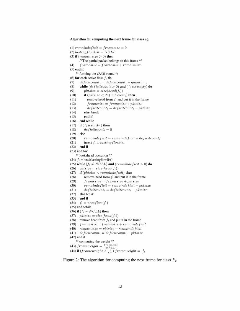
Figure 2 shows the logical algorithm for computing each LDRRWA frame and its weight. In practice,

these frame and weight calculation operations are distributed to the operations in packet arrivals and packet

departures (Appendix B). Table 2 summarizes the major variables in the algorithm. Like DRR, variable

deficitcounti is associated with flow fi to maintain the credits to be passed over to the next DRR round

and decide the amount of data to be sent in one round. After each DRR round, remaindeficit maintains

the sum of the quanta not used in the current DRR round, that is, the quanta that cannot be used since

the size of the next backlogged packet is larger than the remaining quanta for a flow. In traditional DRR,

these unused quanta will be passed to the next DRR round. In LDRRWA, in addition to passing the

unused quanta to the next DRR round, some packets that would be sent in the next DRR round are placed

in the current LDRRWA frame so that at frame boundaries remaindeficit is always equal to 0. This

is the lookahead operation. The lastingflowlist contains the list of flows that are backlogged at the end

of the current DRR round. Flows in lastingflowlist are candidates to supply packets for the lookahead

operation. Frameweight is the weight to be used by inter-class scheduling for the current frame. Variable

framesize records the size of the current frame. Since FRR needs to enforce that remaindeficit = 0 at

frame boundaries, frame boundaries may not align with packet boundaries and a packet may belong to two

frames. Variable remainsize is the size of the part of the last packet in the frame that belongs to the next

frame, and thus, should be counted in the framesize for the next frame.

Let us now examine the algorithm in Figure 2. In the initialization phase, line (1) to line (5), variables are

initialized and remainsize is added to framesize, which effectively includes the partial packet in the frame

to be computed. After the initialization, there are three main components in the algorithm: forming a DRR

round, lookahead operation, and weight calculation. In the first component, line (6) to line (23), the algorithm

puts all packets in the current DRR round that have not been served into the current frame. In the second

component, line (24) to line (42), the algorithm performs the lookahead operation by moving some packets

in the next DRR round into the current frame so that remaindeficit = 0 at the frame boundary. This is

done by allowing some flows to borrow credits from the next DRR round. Since remaindeficit = 0, no

credit is passed from one frame to the next frame for the class that aggregates many flows. Notice that each

backlogged flow can contribute at most one packet in the lookahead operation. Notice also that a class as

14

a whole does not pass credits between frames. However, for an individual flow, credits may still pass from

one frame to the next. As a result, the deficitcounti variable may have a negative or positive value at frame

boundaries. Finally, lines (43) and (44) compute the weight for the frame.

The complexity of the algorithm in Figure 2 is O(M), where M is the number of packets in a frame.

Clearly, this high level algorithm cannot be directly used in a scheduler to determine the next frame and frame

weight. Otherwise, it will introduce an O(M) processing complexity, which is larger than O(N), in a packet

scheduling event since the algorithm goes through each packet in the frame. This algorithm is only used

to illustrate the logical operations of LDRRWA. The operations described in this algorithm, however, can

be realized in the packet-by-packet operations when packets arrive and depart. By distributing the O(M)

operations for determining a frame into M packets in a frame, an additional of O(1) operations are needed in

each packet arrival and departure. In other words, LDDRWA only introduces O(1) per packet processing

overheads.

A detailed description of the packet-by-packet operations of LDRRWA is given in Appendix B, where we

show how to realize LDDRWA with O(1) per packet processing overheads. The detailed packet-by-packet

operations are rather tedious. The idea, however, is straight-forward. LDRRWA maintains active flows in

different queues. To determine a frame and its weight, our scheme determines (1) the total size of the frame,

and (2) for each active flow in the frame the size of the data in that flow that belong to the frame. Such

information is obtained by maintaining the following information at each packet arrival and departure: the

size of the remaining current frame, the size of the next frame, the size of the partial packet in the current

frame, the starting time of the current frame, the deficit counter for each flow, the size of the data for each

flow in the current frame, the size of the data for each flow in the next frame, the size of all backlogged data

in a flow, and the last time that a flow is serviced. Clearly, bookkeeping for all these variables takes O(1)

operations. With such information, the computation of the next frame, as well as the whole LDRRWA can

be realized with O(1) per packet processing overhead.

4.1.2 Properties of LDRRWA

Lemma 3: Assuming that flow fi is continuously backlogged during [t1, t2). Let X be the smallest number of

continuous LDRRWA frames that completely enclose [t1, t2). The service received by fi during this period,

denoted as Si,LDRRWA(t1, t2), is bounded by

15

(X − 3)Qi ≤ Si,LDRRWA(t1, t2) ≤ (X + 1)Qi.

Proof: See appendix. 2

Comparing Lemma 3 and Lemma 1, we can see the similarity between DRR and LDRRWA: in both

schemes, the amount of data sent from a flow fi that is continuously backlogged for X frames (rounds) is a

few packets from X × Qi. Note that Qi in LDRRWA is twice that in DRR.

Lemma 4: In LDRRWA, the weight for a frame is less than or equal to the sum of the weights of all flows

in the class.

Proof: Obvious from the previous discussion. 2

At any given time, let Wk, 1 ≤ k ≤ n be the weights for the n classes (Wk may change over time). Lemma

4 establishes that∑n

i=1 Wk ≤∑N

i=1 wi ≤ 1. Thus, under GPS, the bandwidth allocated to class k is given

by Wk∑n

i=1Wk

R ≥ R × Wk. We will call R × Wk the GPS guaranteed rate.

Lemma 5: Under GPS, the time to serve each LDRRWA frame in class Fk is at most 2CkLM

R .

Proof: Normally, the frame weight is computed as Wk = framesize2CkLM

(line (43) in Figure 2). In cases whenframesize2CkLM

is less than the smallest weight for a flow in a class, the weight is increased (line (44) in Figure 2)

to the smallest weight.

When Wk = framesize2CkLM

, the GPS guaranteed rate is R framesize2CkLM

and the total time to serve the frame is at

most framesize

R framesize

2CkLM

= 2CkLM

R . If Wk is increased, the conclusion still holds. 2

Lemma 6: Under GPS, the time to service X bytes of data in class Fk is at most XCk

R .

Proof: The minimum weight assigned to a backlogged class Fk is 1Ck . Thus, the GPS guaranteed rate for

class Fk is at least RCk . Thus, the time to serve a queue of size X bytes in class Fk is at most X

R

Ck

= XCk

R . 2

Lemma 7: For a class Fk frame of size no smaller than 2LM , the service time for the frame is exactly 2Ck LM

R

using the GPS guaranteed rate.

Proof: When framesize ≥ 2LM , Wk = framesize2CkLM

≥ 1Ck . Thus, the GPS guaranteed rate for the frame is

R framesize2CkLM

and the service time for the frame with the guaranteed rate is framesize

R framesize

2CkLM

= 2CkLM

R . 2

Lemma 8: Let a class Fk frame contain packets of a continuously backlogged flow fi, the size of frame is no

smaller than 2LM .

Proof: Straight-forward from the fact that no credit is passed from the previous frame and to the next frame

and that Qi ≥ 2LM . 2

Lemma 9: Let fi ∈ Fk and fj ∈ Fm be continuously backlogged during [t1, t2). k ≥ m. Let Xk and Xm be

16

the smallest numbers of Fk and Fm frames that completely enclose [t1, t2). Assume that classes Fk and Fm

are served with the GPS guaranteed rate,

(Xk − 1)Ck−m ≤ Xm ≤ XkCk−m + 1.

Proof: Since fi ∈ Fk and fj ∈ Fm are continuously backlogged during [t1, t2), the sizes of all frames during

this period are no smaller than 2LM (Lemma 8). From Lemma 7, using the GPS guaranteed rate, the time

to service a class Fk frame is exactly 2CkLM

R and the time for a class Fm frame is exactly 2CmLM

R . Since Xk

and Xm are the smallest numbers of Fk and Fm frames that completely enclose [t1, t2), we have

t2 − t1 ≤ Xk2CkLM

R ≤ t2 − t1 + 2CkLM

R and t2 − t1 ≤ Xm2CmLM

R ≤ t2 − t1 + 2CmLM

R .

Hence, (Xk − 1)Ck−m ≤ Xm ≤ XkCk−m + 1. 2

Lemma 10: Let fi ∈ Fk and fj ∈ Fm be continuously backlogged during [t1, t2). k ≥ m. Let Xk and Xm

be the smallest numbers of Fk and Fm frames that completely enclose [t1, t2). Assume that the inter-class

scheduler is GPS,

(Xk − 1)Ck−m ≤ Xm ≤ XkCk−m + 1.

Proof: See appendix. 2

f1

f2

f3

Class1

F

Class F2

Class1

F

Class F2

!!!!!!!!!!

""""""""""

4

Frames

weight = 1/2

1 Frames 1 22

weight = 2.01/8

Figure 3: An example

We will use an example to illustrate how LDRRWA interacts with inter-class scheduling to deliver fairness

among flows in different classes. Let us assume that GPS is the inter-class scheduling algorithm. Consider

scheduling for a link with 4 units of bandwidth with the following settings. C = 2 and there are two classes

where F1 = fi : 12 ≤ wi < 1 and F2 = fi : 1

4 ≤ wi < 12. Three flows, f1, f2 and f3, with rates r1 = 2

and r2 = r3 = 1 are in the system. w1 = 1/2, w2 = 1/4, and w3 = 1/4. Thus, f1 is in F1, and f2 and f3

are in F2. Let LM be the maximum packet size. The quantum for each of the three flows is 2LM . All packets

in f1 are of size LM , all packets in f2 are of size 0.99LM and all packets in f3 are of size 0.01LM . Flows f1

17

and f2 are always backlogged. Flow f3 is not always backlogged, its packets arrive in such a way that exactly

one packet arrives before a new frame is to be formed. Thus, each F2 frame contains one packet from f3. The

example is depicted in Figure 3. As shown in the figure, each F1 frame contains exactly two packets from f1.

For F2, the lookahead operation always moves part of the f2 packet in the next DRR round into the current

frame, and thus, the frame boundaries are not aligned with packet boundaries.

The weight for F1 is always 1/2. For F2, the lookahead operation ensures that the size of f2 data in a frame

is 2LM , and thus, the size of each F2 frame is 2LM + 0.01LM = 2.01LM . The weight of F2 is computed as

W2 = framesize2CkLM

= 2.01LM

8LM= 2.01

8 . Hence, F1 (and thus f1) is allocated a bandwidth of 4∗1

21

2+ 2.01

8

= 166.01 > 2.

F2 is allocated a bandwidth of 4 ∗2.018

1

2+ 2.01

8

. For each F2 frame of size 2.01LM , 2LM belongs to f2. Thus, the

rate allocated to f2 is 4 ∗2.018

1

2+ 2.01

8

∗ 2LM

2.01LM= 8

6.01 > 1. The rates allocated to f1 and f2 are larger than their

guaranteed rates and the worst-case fairness is honored. The ratio of the rates allocated to f1 and f2 is equal

to16

6.018

6.01

= 2, which is equal to the ratio of their weights. Thus, the proportional fairness is also honored.

4.2 Inter-class scheduling

LDRRWA assigns different weights for different frames in a class. Moreover, the weight of a frame is

decided only after the last packet in the previous frame is sent. Hence, the inter-class scheduling must be

able to handle these situations while achieving fair sharing of bandwidth. Although GPS can achieve fair

sharing, none of the existing timestamp based schemes can closely approximate GPS under such conditions.

We develop a new scheme called Dynamic Weight Worst-case Fair weighted Fair Queuing (DW 2F 2Q).

DW 2F 2Q has the same scheduling result as WF 2Q [2] when the weights do not change. Theorems presented

later show that the difference between the packet departure times under DW 2F 2Q and GPS is at most

(n−1)LM , where n is the number of classes. This bound is sufficient for FRR to achieve its QoS performance

bounds.

DW 2F 2Q uses the virtual time concept in [12] to track the GPS progress up to the point that it can

accurately track, and schedules packets based on their virtual starting/finishing times. Let us denote an event

in the system the following: (1) the arrival of a packet to the GPS server, (2) the departure of a packet from

the GPS server, and (3) the weight change of a class (LDRRWA may change weight within a packet). Let

tj be the time at which the jth event occurs. Let the time of the first arrival of a busy period be denoted as

t1 = 0. For each j = 2, 3, ..., the set of classes that are busy in the interval [tj−1, tj) is denoted as Bj−1. Let

18

us denote Wk,j−1 the weight for class Fk during the interval [tj−1, tj), which is a fixed value. Virtual time

V (t) is defined to be zero for all times when the system is idle. Assuming that each busy period begins with

time 0, V (t) evolves as follows:

V (0) = 0

V (tj−1 + τ) = V (tj−1) + τ∑k∈Bj−1

Wk,j−1

, 0 < τ ≤ tj − tj−1, j = 2, 3, ...

As discussed in [12], the rate of change of V , ∂V (tj+τ)∂τ , is 1∑

k∈BjWk,j

, and each backlogged class Fk

receives service at rate Wk,j∂V (tj+τ)

∂τ . Let us denote the virtual starting time, virtual finishing time, real

arrival time, and size of the i-th packet P ik in Fk as V start(P i

k), V finish(P ik), arrive(P i

k), and size(P ik),

respectively. Let Wk be the weight for the frame that includes P ik. We have

V start(P ik) = max(V finish(P i−1

k ), V (arrive(P ik)))

V finish(P ik) = V start(P i

k) +size(P i

k)

Wk

DW 2F 2Q keeps track of Bj in order to track the progress of the virtual time. When the last packet in a

frame is sent later than its virtual finishing time (the packet departed under GPS, but not under DW 2F 2Q),

the weight of the class after the frame virtual finishing time is unknown (until the last packet is sent). Hence,

DW 2F 2Q cannot always track the virtual time up to the current time. Before each scheduling decision is

made, DW 2F 2Q tracks the virtual time either to the earliest time when there is a class with an unknown

weight or to the current time when the weights of all classes are known up to the current time. We will

denote this time (the latest time that DW 2F 2Q can track GPS progress accurately) T and the corresponding

virtual time V (T ). Hence, either T is the current time, or there exists one class Fk whose current frame virtual

finishing time is V (T ) and the last packet in that frame has not been sent. DW 2F 2Q only deals with n classes.

As a result, it can afford to recompute timestamps for the first packets in all classes in every scheduling step

without introducing excessive overheads (O(n) = O(1) under our assumption). To ease composition, we

will ignore the issue related to the timing to assign the timestamps to the packets since the timestamps can be

recomputed before each scheduling decision is made. DW 2F 2Q has exactly the same criteria as WF 2Q for

scheduling packets: (1) only packets whose virtual starting times are earlier than the current virtual time are

eligible; and (2) among all eligible packets, the one with the smallest virtual finishing time is selected.

19

There are potentially two problems in DW 2F 2Q. First, determining the virtual finishing time for the last

packet in a frame can be a problem when only a part of the packet belongs to the current frame. The weight

for the part of the packet in the next frame is unknown until the packet is scheduled. DW 2F 2Q assigns the

frame virtual finishing time as the packet virtual finishing time for this type of packets. Although this creates

some inaccuracy, the scheduling results are still sufficiently good as will be shown later.

The other problem is that T may not be the current time and the virtual time corresponding to the current

time is unknown. In this case, there must exist one class Fk whose current frame virtual finishing time is

V (T ) and the last packet in that frame, P , has not been sent. The virtual finishing time (and the virtual

starting time) of P must be less than or equal to V (T ). Since DW 2F 2Q has accurate virtual time up to

time T , the timestamps for all packets with finishing times less than V (T ) are available. All unknown virtual

finishing times for packets must be larger than V (T ). In this case, the packet to be scheduled must have a

virtual finishing time less than or equal to V (T ). Hence, DW 2F 2Q can simply assign a large timestamp

as the virtual finishing time for packets with unknown virtual finishing times (to prevent these packets to

be scheduled) and only consider packets whose virtual finishing time is less than or equal to V(T) when

T is less than the current time. Not being able to tracking virtual time up to the current time does not

prevent DW 2F 2Q from selecting the right packet for transmission. Note that when T equals the current

time, DW 2F 2Q schedules packets exactly like WF 2Q.

The packet-by-packet operations of DW 2F 2Q are given in Appendix B, where we show that the worst-

case per packet scheduling complexity is O(nlg(n)). In practical cases, n = O(1) and hence, the per packet

complexity of DW 2F 2Q is also O(1). The following theorems shows properties of DW 2F 2Q.

Theorem 1: DW 2F 2Q is work conserving.

Proof: See appendix. 2

Since both GPS and DW 2F 2Q are work-conserving disciplines, their busy periods coincide. We will

consider packet scheduling within one busy period. Let F ki,s be the departure time of the kth packet in class i

under server s in a busy period.

Lemma 11: If F ki,GPS ≤ F m

j,GPS , F ki,DW 2F 2Q < F m+1

j,DW 2F 2Q.

Proof: Let pli be the packet at the head of class i at time t when pm+1

j is at the head of class j and is eligible

to be transmitted. Let the timestamp assigned to pm+1j be V T , we have V T > V (F m

j,GPS). This applies even

when pm+1j is the last packet in a frame and is assigned an inaccurate timestamp.

20

If l > k, we have F ki,DW 2F 2Q < F m+1

j,DW 2F 2Q and the lemma is proved. If l ≤ k, F li,GPS < F l+1

i,GPS < ... <

F ki,GPS ≤ F m

j,GPS and V (F li,GPS) < V (F l+1

i,GPS) < ... < V (F ki,GPS) ≤ V (F m

j,GPS) < V T . For a packet

pXi that is in the frame boundary, its timestamp is less than or equal to V (F X

i,GPS). Since at time t, pm+1j

is eligible for scheduling, V (t) ≥ V (F mj,GPS) and the accurate virtual times for these packets are available,

all of these packets have smaller virtual starting and finishing times than pm+1j and will depart before pm+1

j

under DW 2F 2Q. Thus, F ki,DW 2F 2Q < F m+1

j,DW 2F 2Q. 2

Lemma 11 indicates that DW 2F 2Q can at most introduce one packet difference between any two classes

in comparison to GPS. This leads to the following theory that states relation of GPS departure time and

DW 2F 2Q departure time. Let F ps be the time packet p departs under server s.

Theorem 2: Let n be the number of classes in the system,

F pDW 2F 2Q − F p

GPS ≤ (n − 1)LM

R .

Proof: Consider any busy period and let the time that it begins be time zero. Let pk be the kth packet of

size sk to depart under GPS. We have F pk

GPS ≥ s1+s2+...+sk

R . Now consider the departure time of pk under

DW 2F 2Q. From Lemma 11, each class can have at most one packet whose GPS finishing time is after packet

pk and whose DW 2F 2Q finishing time is before packet pk. Hence, there are at most n− 1 packets (from the

n−1 other classes) that depart before packet pk under DW 2F 2Q and have a GPS finishing time after F pk

GPS .

Let the n−1 packets be e1, e2, ..., en−1 with sizes se1, se2, ..., sen−1. All other packets depart before pk under

DW 2F 2Q must have GPS finishing times earlier than F pk

GPS . We have F pk

DW 2F 2Q ≤ s1+...+sk+se1+...+sen−1

R .

Thus, F pk

DW 2F 2Q − F pk

GPS ≤ (n − 1)LM

R . 2

Theorem 2 indicates that, under the assumption that n is a small constant, the difference in the packet

departure times under DW 2F 2Q and GPS is within a constant number of packets.

5 Properties of FRR

This session formally analyzes the QoS properties of FRR. We will prove that the three statements in Lemma

2 hold for FRR with an arbitrary weight distribution. As will be shown in the following theorems, even when

the weight different factor D is large or related to N (e.g. D = O(N)), using FRR, one can select a constant

C (e.g. C = 2) that is independent of D or N and enjoy QoS performance bounds that are linear functions of

C and n. As discussed earlier, we consider practical cases when n is an O(1) constant, but will express the

21

bounds in terms of C and n.

Theorem 3 (single packet delay bound): Let packet p arrives at the head of flow fi ∈ Fk at time t. Using

FRR, there exists a constant c1 (c1 = O(C + n)), such that p will depart before t + c1 ∗LM

ri.

Proof: If class Fk is idle under GPS at time t, a new frame that includes packet p will be formed at time t.

From Lemma 5, under GPS, the frame will be served at most at time t+2C k LM

R ≤ t+2C LM

ri. Hence, from

Theorem 2, the frame will be served under DW 2F 2Q before t+2C LM

ri+(n−1)LM

R ≤ t+(2C +n−1)LM

ri,

where n is the number of classes in the system. Thus, there exists c1 = 2C + n − 1 = O(C + n) such that

packet departs before t + c1 ∗LM

ri.

If class Fk is busy under GPS at time t, packet p will be included in the next frame. From Lemma 5,

F pGPS ≤ t + 2 ∗ 2LM Ck

R ≤ t + 4CLM

ri. From Theorem 2, the frame will be served under DW 2F 2Q before

t + 4C LM

ri+ (n− 1)LM

R ≤ t + (4C + n− 1)LM

ri. Thus, there exists c1 = 4C + n− 1 = O(C + n) such that

packet p departs before t + c1 ∗LM

ri. 2

Theorem 4 (worst-case fairness): FRR has a constant (O(C + n)) normalized worst-case fairness index.

Proof: Let a packet belonging to flow fi ∈ Fk arrive at time t, creating a total backlog of qi bytes in fi’s queue.

Let packet p1 be the first packet in the backlog. From the proof of Theorem 3, we have F p1

GPS ≤ t + 4C LM

ri.

After the first packet is served under GPS, from Lemma 3, at most d qi

Qie+3 ≤ qi

Qi+4 frames will be needed

to drain the queue. From Lemma 5, under GPS, servicing the qi

Qi+ 4 frames will take at most

( qi

Qi+ 4) ∗ 2Ck LM

R = qi

CkwiLM

CkLM

R + 8Ck LM

R ≤ qi

ri+ 8C LM

ri

Thus, under GPS, the queue will be drained before t + qi

ri+ 4C LM

ri+ 8C LM

ri. From Theorem 2, under

DW 2F 2Q, the queue will be drained before t + qi

ri+ 12C LM

ri+ (n − 1)LM

R . Thus, there exists a constant

d = 12C + n − 1 = O(C + n) such that the queue will be drained before t + qi

ri+ dLM

riand the normalized

worst-case fair index for FRR is maxiri∗d

LMri

R = dLM

R . 2

The normalized worst-case fair index for FRR is (12C + n − 1) LM

R . While this constant is still quite

large, it significantly improves over STRR whose index is Ω(N). Next we will consider FRR’s proportional

fairness.

Lemma 12: Assuming that fi ∈ Fk and fj ∈ Fm are continuously backlogged during [t1, t2), k ≥ m.

Assume that the inter-class scheduler is GPS and the intra-class scheduler is LDRRWA. Let Si(t1, t2) be

the services given to flow fi during [t1, t2) and Sj(t1, t2) be the services given to flow fj during [t1, t2). There

22

exists two constants c1 and c2 (c1 ≤ O(C) and c2 ≤ O(C)) such that

|Si(t1, t2)

ri−

Sj(t1, t2)

rj| ≤

c1 ∗ LM

ri+

c2 ∗ LM

rj.

Proof: Let Xk and Xm be the smallest numbers of Fk and Fm frames that completely enclose [t1, t2). Since

fi and fj are continuously backlogged during the [t1, t2) period, from Lemma 3, the services given to fi and

fj during this period satisfy:

(Xk − 3)Qi ≤ Si(t1, t2) ≤ (Xk + 1)Qi and (Xm − 3)Qj ≤ Sj(t1, t2) ≤ (Xm + 1)Qj .

The conclusion follows by manipulating these in-equations and applying Lemma 10, which gives the rela-

tion between Xk and Xm, (Xk − 1)Ck−m ≤ Xm ≤ XkCk−m + 1.

In the following, we will derive the bound for Si(t1,t2)ri

−Sj(t1,t2)

rj.

Si(t1,t2)ri

−Sj(t1,t2)

rj≤ (Xk+1)Qi

ri−

(Xm−3)Qj

rj≤ QiXk

ri−

QjXm

rj+ Qi

ri+

3Qj

rj

≤ QiXk

ri−

Qj(Xk−1)Ck−m

rj+ 2CLM

ri+ 6CLM

rj

= QiXk

ri−

Qj(Xk)Ck−m

rj+

QjCk−m

rj+ 2CLM

ri+ 6CLM

rj

We have QjCk−m

rj=

CmwjLMCk−m

wjR ≤ C∗LM

riand QiXk

ri−

Qj(Xk)Ck−m

rj= CkwiLM Xk

wiR−

CmwjLMXkCk−m

wjR =

0. Thus, Si(t1,t2)ri

−Sj(t1 ,t2)

rj≤ 3CLM

ri+ 6CLM

rj. The bound for Sj(t1,t2)

rj−Si(t1 ,t2)

rican be derived in a similar

fashion. Hence, there exists two constants c1 and c2, c1 = O(C) and c2 = O(C), such that |Si(t1,t2)ri

−

Sj(t1 ,t2)rj

| ≤ c1∗LM

ri+ c2∗LM

rj.2

Lemma 12 shows that if GPS is used as the inter-class scheduling algorithm, the scheduling algorithm

provides proportional fairness. Since DW 2F 2Q closely approximates GPS (at most one packet can be out-

of-order between any two classes (Lemma 11)), we will show in the next theorem that FRR, which uses

DW 2F 2Q as the inter-class scheduling algorithm, also supports proportional fairness.

Theorem 5 (proportional fairness): In any time period [t1, t2) during which flows fi ∈ Fk and fj ∈ Fm

are continuously backlogged in FRR. There exists two constants c1 = O(C) and c2 = O(C) such that

|Si,FRR(t1 ,t2)

ri−

Sj,FRR(t1 ,t2)rj

| ≤ c1∗LM

ri+ c2∗LM

rj.

Proof: See appendix. 2

23

6 Simulation experiments

We compare FRR with Weighted Fair Queueing (WFQ) and two recently proposed deficit round robin

(DRR) based schemes, Smoothed Round Robin (SRR) [7] and STratified Round Robin (STRR) [13]. All

experiments are performed using ns-2 [11], to which we added WFQ, STRR, and FRR queuing classes.

Figure 4 shows the network topology used in the experiments. All links have a bandwidth of 2Mbps and

a propagation delay of 1ms. In all experiments, CBR flows have a fixed packet size of 210 bytes, and all

other background flows have a fixed packet size uniformly chosen between 128 and 1024 bytes. Except for

the experiment summarized in Figure 8 where only CBR and deterministic flows are considered, for all other

experiments, we report the results using the confidence interval with a 99% confidence level.

S0 N1

S1 S2

R1

R0N2 N3

R2

Figure 4: Simulated network.

Figure 5 shows the average end-to-end delays for flows with different rates. Figure 6 shows the worst-case

end-to-end delays. In the experiment, there are 10 CBR flows from S0 to R0 with average rates of 10Kbps,

20Kbps, 40Kbps, 60Kbps, 80Kbps, 100Kbps, 120Kbps, 160Kbps, 200Kbps, and 260Kbps. The average

packet delays of these CBR flows are measured. The background traffic in the system is as follows. There are

five exponential on/off flows from S1 to R1 with rates 60Kbps, 80Kbps, 100Kbps, 120Kbps, and 160Kbps.

0 10 20 30 40 50 60 70 80 90

100 110

0 50 100 150 200 250 300

aver

age

pack

et d

elay

(m

s)

flow rate (Kbps)

SRRSTRR

FRRWFQ

Figure 5: Average end-to-end delay.

0 50

100 150 200 250 300 350 400 450 500

0 50 100 150 200 250 300

wor

st-c

ase

pack

et d

elay

(m

s)

flow rate (Kbps)

SRRSTRR

FRRWFQ

Figure 6: Worst-case end-to-end delay

24

The on-time and the off-time are 0.5 second. There are five Pareto on/off flows from S2 to R2 with rates

60Kbps, 80Kbps, 100Kbps, 120Kbps, and 160Kbps. The on-time and the off-time are 0.5 second. The

shape parameter of the Pareto flows is 1.5. Two 7.8Kbps FTP flows with infinite traffic are also in the system,

one from S1 to R1 and the other one from S2 to R2.

0

100

200

300

400

500

7000 6000 5000 4000 3000

thro

ughp

ut (

Kbp

s)

time (ms)

STRR

(a) STRR

0

100

200

300

400

500

7000 6000 5000 4000 3000

thro

ughp

ut (

Kbp

s)

time (ms)

FRR

(b) FRR

0

100

200

300

400

500

7000 6000 5000 4000 3000

thro

ughp

ut (

Kbp

s)

time (ms)

WFQ

(c) WFQ

Figure 7: Short-term throughput

In this experiment, all of the three deficit round-robin based schemes, SRR, STRR, and FRR, give

reasonable approximation of WFQ for all the flows with different rates. In comparison to SRR and STRR,

FRR achieves average and worst-case end-to-end delays that are closer to the ones for WFQ for flows with

large rates (≥ 150Kbps in the experiment). In FRR, the timestamp based inter-class scheduling mechanism

is added on top of DRR so that flows with small rates do not significantly affect flows with large rates. Thus,

in a way, FRR gives preference to flows with larger weights in comparison to other DRR bases schemes.

Figure 7 (a), (b), and (c) shows the short-term throughput achieved by different schemes. Since the results

for SRR are very similar to those for STRR, we only show the results for STRR. In this experiment, the

short-term throughput in an interval of 100ms is measured. We observe one 300Kbps CBR flow and one

600Kbps flow from S0 to R0. In addition, 50 10Kbps CBR flows from S0 and R0 are introduced. Other

background flows are the same as the previous experiment.

Figure 7 (a), (b), and (c) shows the results for the 300 Kbps flow. The results for the 600 Kbps flow have

a similar trend. As can be seen from the figure, the short term throughput for STRR (and SRR) exhibit

heavy fluctuations. On the other hand, WFQ and FRR yield much better short term throughput: within each

interval of 100ms, the throughput is always close to the ideal rate. This demonstrates that FRR has a much

better short-term fairness property than SRR and STRR.

Figure 8 shows the proportional fairness of FRR. In this experiment, we observe four deterministic flows

25

0

200

400

600

800

1000

1200

10 11 12 13 14 15 16 17 18 19

thro

ughp

ut (

Kbp

s)

time (second)

100 Kbps200 Kbps (1)200 Kbps (2)

300 Kbps

Figure 8: Proportional fairness

0

100

200

300

400

500

600

700

800

900

0 20 40 60 80 100 120 140 160

wor

st c

ase

pack

et d

elay

(m

s)

flow rate (kbps)

C = 2C = 4C = 8

Figure 9: Worst-case end-to-end delay.

0

2

4

6

8

10

12

14

0 20 40 60 80 100 120 140 160D

elay

in m

axim

um s

ized

pac

kets

flow rate (Kbps)

C = 2C = 4C = 8

Figure 10: Delay in terms of numbers of packets

from S0 to R0 with average rates of 100Kbps, 200Kbps, 200Kbps, and 300Kbps. These flows follow an

off/on pattern with each off/on period being 10 seconds. Hence, the flows are quiet for 10 seconds and then

send in a doubled rate for the next 10 seconds. One 600Kbps CBR flow from S1 to R1 is introduced in period

[10s, 16s] and another 400Kbps CBR flow from S1 to R1 is introduced in period [12s, 14s]. The CBR flows

and the observed flows share the link from N1 to N2. The bandwidth allocation in the link from N1 to N2

to each of the flows during period [10s, 19s] is showed in Figure 8. As can be see from the figure, for all

periods with different traffics sharing the link, the bandwidth allocation to the four observed flows is exactly

proportional to their reserved bandwidths.

The last experiment is designed to study the impacts of C , a parameter in FRR. The background traffics

used in this experiment are the same as those in Figure 5. We observe the worst case end-to-end packet

delay for 16 CBR flows from S0 to R0 with average rates of 10Kbps, 20Kbps, 30Kbps, 40Kbps, 50Kbps,

60Kbps, 70Kbps, 80Kbps, 90Kbps, 100Kbps, 110Kbps, 120Kbps, 130Kbps, 140Kbps, 150Kbps, and

160Kbps. When C = 8, there are two classes in the system, F3 containing flows with rates 10Kbps, 20Kbps,

26

and 30Kbps, and F2 containing the rest of the flows. When C = 4, there are three classes in the system, F4

(10Kbps to 30Kbps), F3 (40Kbps to 120Kbps), and F2 (130Kbps to 160Kbps). When C = 2, there are 5

classes: F8 (10Kbps), F7 (20Kbps and 30Kbps), F6 (40Kbps to 60Kbps), F5 (70Kbps to 120Kbps), and

F4 (130Kbps to 160Kbps).

Figure 9 shows the worst case delay in milli-seconds. We can see that the worst case delay for flows within

one class are similar, which is evidenced by the ladder shape curves in the figure. This is expected as the

DRR based scheme is used for intra-class scheduling. The packet delay is directly related to C . A smaller C

value results in a smaller worst case packet delay.

Figure 10 shows a different view of Figure 9. In this figure, we represent the absolute worst case delay time

as the time to send a number of packets (packets are of the same size, 210B, in this experiment). This allows

the delay to be normalized by the flow rate. There are two interesting observations in Figure 10. First, within

each class, FRR biases against flows with larger weights. This is due to the use of a DRR based scheme

for intra-class scheduling. Biasing against flows with large weights is a common problem for all DRR based

schemes. However, in FRR, this problem is limited since the weight difference within a class is bounded.

Second, FRR treats different classes fairly. It can be seen that for flows in different classes, the worst case

packet delays fall in ranges with similar lower bounds and upper bounds as shown in the seesaw shape curve

(e.g. when C = 2).

7 Conclusion

In this paper, we describe Fair Round Robin (FRR), a low quasi-O(1) complexity round robin scheduler

that provides proportional and worst-case fairness. In comparison to other DRR based scheduling schemes,

FRR has similar complexity and proportional fairness, but better worst-case fairness. The simulation study

demonstrates that even in average cases, FRR has better short-term behavior than other DRR based schemes,

including smoothed round robin and stratified round robin. The constant factors in the complexity and QoS

performance bounds for FRR are still fairly large. Recent improvements on GPS tracking [19, 20, 23] and

DRR implementations [8] may be applied to improve FRR.

27

References

[1] J. Bennett and H. Zhang, “Hierarchical Packet Fair Queueing Algorithms,” ACM/IEEE Trans. on Networking,

5(5):675-689, Oct. 1997.

[2] J. Bennett and H. Zhang, “WF 2Q: Worst Case Fair Weighted Fair Queuing”, in IEEE INFOCOM’96 (1996),

pages 120-128.

[3] B. Caprita, J. Nieh, and W. Chan, “Group Round Robin: Improving the Fairness and Complexity of Packet

Scheduling.” Proceedings of the 2005 Symposium on Architecture for Networking and Communications Systems

(ANCS’05), Princeton, New Jersey, 2005.

[4] S.Cheung and C. Pencea, “BSFQ: Bin Sort Fair Queuing,” in IEEE INFOCOM’02 (2002), pages 1640-1649.

[5] A. Demers, S. Keshav, and S. Shenker, “Analysis and Simulation of a Fair Queuing Algorithm,” in ACM SIG-

COMM’89 (1989), pages 1-12.

[6] S. Golestani, “A Self-clocked Fair Queueing Scheme for Broadband Applications”, in IEEE INFOCOM’94 (1994),

pages 636-646.

[7] C. Guo, “SRR, an O(1) Time Complexity Packet Scheduler for Flows in MultiService Packet Networks,”

IEEE/ACM Trans. on Networking, 12(6):1144-1155, Dec. 2004.

[8] L. Lenzini, E. Mingozzi, and G. Stea, “Aliquem: a Novel DRR Implementation to Achieve Better Latency and

Fairness at O(1) Complexity,” in IWQoS’02 (2002), pages 77-86.

[9] L. Lenzini, E. Mingozzi, and G. Stea, “Tradeoffs Between Low Complexity, Low Latency, and Fairness with

Deficit Round-Robin Schedulers.” IEEE/ACM Trans. on Networking, 12(4):681-693, April 2004.

[10] L. Massouli and J. Roberts, “Bandwidth Sharing: Objectives and Algorithms,” IEEE/ACM Trans. on Networking,

10(3):320-328, June 2002.

[11] “The Network Simulator - ns-2,” available at http://www.isi.edu/nsnam/ns.

[12] A. Parekh and R. Gallager, “A Generalized Processor Sharing Approach to Flow Control in Integrated Services

Networks: the Single Node Case,” IEEE/ACM Trans. on Networking, 1(3):344-357, June 1993.

[13] S. Ramabhadran and J. Pasquale, “The Stratified Round Robin Scheduler: Design, Analysis, and Implementation.”

IEEE/ACM Transactions on Networking, 14(6):1362-1373, Dec. 2006.

[14] J. Rexford and A. Greenberg and F. Bonomi, “Hardware-Efficient Fair Queueing Architectures for High-Speed

Networks,” IEEE INFOCOM’96, (1996), pages 638-646.

28

[15] J. L. Rexford, F. Bonomi, A. Greenberg, A. Wong, “A Scalable Architecture for Fair Leaky-Bucket Shaping,” in

INFOCOM’97 (1997), pages 1056–1064.

[16] D. Stiliadis and A. Varma, “Design and Analysis of Frame-based Fair Queueing: A New Traffic Scheduling

Algorithm for Packet-Switched Networks,” in ACM SIGMETRICS’96 (1996), pages 104-115.

[17] M. Shreedhar and G. Varghese, “Efficient Fair Queuing using Deficit Round Robin,” in ACM SIGCOMM’95

(1995), pages 231-242.

[18] S. Suri, G. Varghese, and G Chandranmenon, “Leap Forward Virtual Clock: An O(loglog N) Queuing Scheme

with Guaranteed Delays and Throughput Fairness,” in IEEE INFOCOM’97 (1997), pages 557-565.

[19] P. Valente, “Exact GPS Simulation with Logarithmic Complexity, and its Application to an Optimally Fair Sched-

uler,” in ACM SIGCOMM’04 (2004), pages 269-280.

[20] J. Xu and R. J. Lipton, “On Fundamental Tradeoffs between Delay Bounds and Computational Complexity in

Packet Scheduling Algorithms,” in ACM SIGCOMM’02 (2002), pages 279-292.

[21] X. Yuan and Z. Duan, “FRR: a Proportional and Worst-Case Fair Round Robin Scheduler,” IEEE INFOCOM,

pages 831-842 (Vol. 2), Miami, March 13-17, 2005.

[22] L. Zhang, “Virtual Clock: A New Traffic Control Scheme for Packet Switching Networks”, in ACM SIGCOMM’90

(1990), pages 19-29.

[23] Q. Zhao and J. Xu, “On the Computational Complexity of Maintaining GPS Clock in Packet Scheduling,” in IEEE

INFOCOM’04 (2004), pages 2383-2392.

Appendix A: Proofs

Lemma 1: Assuming that flow fi is backlogged during [t1, t2). Let X be the smallest number of continuous

DRR rounds that completely enclose [t1, t2). The service received by fi during this period, Si,DRR(t1, t2), is

given by

(X − 3)quantumi ≤ Si,DRR(t1, t2) ≤ (X + 1)quantumi.

Proof: Since X is the smallest number of continuous DRR rounds that completely enclose [t1, t2), fi is served

in at least X − 2 rounds. Thus, Si,DRR(t1, t2) ≥ (X − 2) ∗ quantumi − LM ≥ (X − 3)quantumi since

we assume that quantumi ≥ LM . On the other hand, fi is served in at most all X rounds, in this case, the

total number of data sent should be less than the total quantum generated during the rounds plus the left over

29

from the previous DRR round, which is less than LM . Thus, Si,DRR(t1, t2) ≤ X ∗ quantumi + LM ≤

(X + 1)quantumi. 2

Lemma 2: Let f1, ..., fN be the N flows in the system with guaranteed rates r1, ...,rN .∑N

i=1 ri ≤ R. Let

rmin = miniri and rmax = maxiri. Let rmax = D ∗ rmin. Assume that D is a constant with respect to

N and that DRR is used to schedule the flows with Qi = LM ∗ ri

rmin. The following statements are true. All

constants in this lemma are with respect to N .

1. Let packet p arrive at the head of the queue for fi at time t. There exists a constant c1 (c1 = O(D2))

such that packet p will be serviced before t + c1 ×LM

ri.

2. The normalized worst-case fair index of DRR in such a system is a constant c1 (c1 = O(D2)).

3. Let fi and fj be continuously backlogged during any given time period [t1, t2), there exists two con-

stants c1 and c2 (c1 = O(D) and c2 = O(D)) such that the normalized service received by the two

flows during this period is bounded by |Si,DRR(t1,t2)

ri−

Sj,DRR(t1 ,t2)rj

| ≤ c1LM

ri+ c2

LM

rj.

Proof: Since N ∗ rmin ≤ r1 + r2 + ... + rN ≤ R, rmin ≤ RN . quantumi = LM ∗ ri

rmin≤ D ∗LM . Thus, the

total size of a round is at most∑N

i=1quantumi +LM ≤ (D+1)∗N ∗LM . The time to complete service in

a round is at most (D+1)N∗LM

R ≤ (D+1)∗ LM

rmin≤ (D+1)∗ LM

rmax/D = D(D+1)∗ LM

rmax≤ D(D+1)∗ LM

ri.

Packet p arrives at the head of the queue for fi time t. It takes at most two rounds for the packet to be

serviced. There exists a constant c1 = 2 ∗ D(D + 1) = O(D2) such that packet p will be serviced before

t + c1 ×LM

ri. This proves the first statement. Next, we will prove the second statement.

Let a packet belonging to flow fi arrives at time t, creating a total backlog of size qi in fi’s queue. From

statement 1., there exists a constant c1 such that the first packet in the queue will be serviced in t + c1 ×LM

ri.

After the first packet is serviced, there will be at most d qi

quantumie + 1 ≤ qi

quantumi+ 2 rounds for the qi data

to be sent. During the qi

quantumi+ 2 rounds, at most ( qi

quantumi+ 2) ∗

∑Nj=1 quantumj quanta are generated,

and thus, at most ( qi

quantumi+2) ∗

∑Nj=1 quantumj +N ∗LM data are sent since each flow can have at most

LM credits left from the previous round. Thus, the total time to complete the qi

quantumi+ 2 rounds is at most

(qi

quantumi+2)∗

∑N

j=1quantumj+N∗LM

R = ( qi

quantumi+ 2)

∑N

j=1quantumj

R + N∗LM

R

= ( qi

quantumi+ 2)

∑N

j=1LM∗

rj

rmin

R + N∗LM

R

= ( qi

quantumi+ 2) LM

rmin

∑N

j=1rj

R + N∗LM

R

30

≤ ( qi

quantumi+ 2) LM

rmin+ N∗LM

R ≤ ( qi

LM∗ri

rmin

) LM

rmin+ 3LM

rmin

≤ qi

ri+ 3∗LM

rmin≤ qi

ri+ 3∗LM

rmax/D ≤ qi

ri+ 3D∗LM

ri

Thus, there exists a constant c2 = c1 + 3D = O(D2) such that the queue of size qi will be sent before

t+ qi

ri+c2∗

LM

ri. This is true for all flows. The normalzied worst case fair index is cDRR = maxi

riCi,DRR

R =

c2LM

R . This proves the second statement.

For any given time period, [t1, t2), let fi and fj be backlogged during this period that is enclosed by X

rounds. From Lemma 1, we have

(X − 3)quantumi ≤ Si,DRR(t1, t2) ≤ (X + 1)quantumi

(X − 3)quantumj ≤ Sj,DRR(t1, t2) ≤ (X + 1)quantumj

By manipulating these inequations, it can be shown that there exist two constants c1 = c2 = 4D = O(D),

such that |Si,DRR(t1 ,t2)ri

−Sj,DRR(t1,t2)

rj| ≤ c1

LM

ri+ c2

LM

rj. 2

Lemma 3: Assuming that flow fi is continuously backlogged during [t1, t2). Let X be the smallest number of

continuous LDRRWA frames that completely enclose [t1, t2). The service received by fi during this period,

denoted as Si,LDRRWA(t1, t2), is bounded by

(X − 3)Qi ≤ Si,LDRRWA(t1, t2) ≤ (X + 1)Qi.

Proof: The notation Si,LDRRWA(t1, t2) is abused in this lemma since LDRRWA does not decide the actual

timing to service packets. In this lemma, Si,LDRRWA(t1, t2) denotes the amount of data for a continuously

backlogged flow fi in X continuous LDRRWA frames (of a particular class) using any inter-class scheduling

scheme.

Since fi is continuously backlogged, it will try to send as many packets as possible in each frame. Since

X frames enclose [t1, t2), flow fi will fully utilize at least X − 2 frames (all but the first frame and the last

frame). In the X − 2 frames, (X − 2) × Qi credits are generated for flow fi. The lookahead operation in

the frame prior to the X − 2 frames may borrow at most one packet, whose size is less than LM , from fi in

the first of the X − 2 frames and flow fi in the last of the X − 2 frames may pass at most LM credits to the

next frame. Note that the lookahead operation borrows at most one packet from each backlogged flow. Thus,

Si,LDRRWA(t1, t2) ≥ (X − 2) × Qi − LM − LM . Since Qi ≥ 2LM , Si,LDRRWA(t1, t2) ≥ (X − 3) × Qi.

On the other hand, fi will be served in at most all the X frames, which produces X × Qi credits for fi

during this period of time. Flow fi in the frame prior to the X frames may have at most LM left-over credits

31

and the lookahead operation in the last of the X frames may borrow at most LM credits from fi in the next

frame. Thus,

Si,LDRRWA(t1, t2) ≤ X × Qi + LM + LM ≤ (X + 1)Qi.2

Lemma 10: Let fi ∈ Fk and fj ∈ Fm be continuously backlogged during [t1, t2). k ≥ m. Let Xk and Xm

be the smallest numbers of Fk and Fm frames that completely enclose [t1, t2). Assume that the inter-class

scheduler is GPS,

(Xk − 1)Ck−m ≤ Xm ≤ XkCk−m + 1.

Proof: This lemma relaxes the condition in Lemma 10 by not requiring each class to be serviced with its

GPS guaranteed rate. Since fi ∈ Fk and fj ∈ Fm be continuously backlogged during [t1, t2), the sizes of

all frames during this period are no smaller than LM (Lemma 9). Let us partition the duration [t1, t2) into

smaller intervals [a1 = t1, b1), [a2 = b1, b2), ..., [aY = bY −1, bY = t2) such that within each interval [ah, bh),

1 ≤ h ≤ Y , the weights of all classes are fixed. Let F1, ..., Fn be the n classes in the system. Let class Fk

have weight whk during interval [ah, bh), 1 ≤ h ≤ Y (If Fk is not backlogged, wh

k = 0). The amount of class

Fk data sent during [ah, bh) is thus,wh

k∑ni=1 wh

i

R ∗ (bh − ah).

Consider a reference scheduling system that contains three classes RFk, RFm, and RFo. Let us use

intervals [aa1 = t1, bb1), [aa2 = bb1, bb2), ..., [aaY = bbY −1, bbY ) to emulate the behavior of classes Fk and

Fm during intervals [a1 = t1, b1), [a2 = b1, b2), ..., [aY = bY −1, bY ) respectively. Let rwhk be the weight

for class RFk during interval [aah, bbh), 1 ≤ h ≤ Y . Let rwhm be the weight for class RFm during interval

[aah, bbh), 1 ≤ h ≤ Y . Let rwho be the weight for class RFo during interval [aah, bbh), 1 ≤ h ≤ Y . The

weights and the duration of each interval are given as follows:

rwhk = wh

k , rwhm = wh

m, rwho = 1 − wh

k − whm, 1 ≤ h ≤ Y

and

bbh = aah +bh − ah∑n

i=1 whi

, 1 ≤ h ≤ Y.

It can be verified that the amount of classes RFk and RFm data sent in an interval [aah, bbh), 1 ≤ h ≤ Y , is

exactly the same as the amount of classes Fk and Fm data sent in an interval [ah, bh), 1 ≤ h ≤ Y , respectively.

32

In an interval [aah, bbh), 1 ≤ h ≤ Y , let us further assume that Class RFk has exactly the same sequence of

packets as Class Fk has in interval [ah, bh) and that Class RFm has exactly the same sequence of packets as

Class Fm has in interval [ah, bh). The progress of classes Fk and Fm during [t1, t2) is exactly the same as the

progress of class RFk and RFm during [aa1, bbY )

In the reference system, classes RFm and RFk are serviced with the GPS guaranteed rate during [aa1, bbY ).

Let RXk and RXm be the smallest numbers of RFk and RFm frames that completely enclose [aa1, bbY ).

From Lemma 10, (RXk − 1)Ck−m ≤ RXm ≤ RXkCk−m + 1.

Let Xk and Xm be the smallest number of Fk and Fm frames that completely enclose [t1, t2). Since the

progress of classes Fk and Fm during [t1, t2) is exactly the same as the progress of class RFk and RFm during

[aa1, bbY ), we have Xk = RXk and Xm = RXm. Thus, (Xk − 1)Ck−m ≤ Xm ≤ XkCk−m + 1. 2

Theorem 1: DW 2F 2Q is work conserving.

Proof: Since GPS is work-conserving, we will prove the theorem by showing that DW 2F 2Q has the same

idle and busy periods as GPS. Assuming that DW 2F 2Q and GPS have different idle and busy periods. Let

t be the first occurrence when GPS and DW 2F 2Q are not in the same state. There are two cases.

Case 1: GPS is idle and DW 2F 2Q is busy, serving packet p. Since t is the first occurrence when GPS

and DW 2F 2Q are not in the same state, the amount of data served during [0, t) must be the same for the

two scheduling schemes. Since p is currently being served under DW 2F 2Q, p must be started before t under

GPS. Since GPS is idle at time t, packet p must finish before t under GPS. Hence, there must exist a packet

q such that q has not been served under GPS during [0, t) and has been served by DW 2F 2Q during [0, t).

Since GPS is idle at t, packet q should start after t under GPS, which indicates that q cannot be served under

DW 2F 2Q during [0, t). This is the contradiction.

Case 2: GPS is busy and DW 2F 2Q is idle. Let packets p1, p2, ..., pi be the packets departed under GPS

during [0, t) and packets cp1, ..., cpj be the packets currently in progress under GPS. Since GPS is busy, at

least one packet is being serviced at time t. Since DW 2F 2Q is idle at t, all packets that starts before t under

GPS should have been served, that is, packets p1, p2, ..., pi and cp1, ..., cpj are all served during [0, t) under

DW 2F 2Q. Thus, during [0, t), DW 2F 2Q sends more data than GPS and t cannot be the first occurrence

that GPS and DW 2F 2Q are not in the same state. 2

Theorem 5 (proportional fairness): In any time period [t1, t2) during which flows fi ∈ Fk and fj ∈ Fm

are continuously backlogged in FRR. There exists two constants c1 = O(C) and c2 = O(C) such that

33

|Si,FRR(t1 ,t2)

ri−

Sj,FRR(t1 ,t2)rj

| ≤ c1∗LM

ri+ c2∗LM

rj.

Proof: There are two cases. The first case is when flows fi and fj are in the same class, that is, k = m. The

second case is when flows fi and fj are not in the same class, that is, k 6= m. The proof of the first case is

similar to the proof of the statement 3 in Lemma 2. Here, we will focus on the second case. Let us assume

that k > m.

Let packets p1k, p2

k, ..., pak be the sequence of class Fk packets sent under FRR during [t1, t2). Let packets

p1m, p2

m, ..., pbm be the sequence of class Fm packets sent under FRR during [t1, t2). Since flows fi and fj are

continuously backlogged during [t1, t2), there exists a packet p0k that departed before p1

k and pa+1k that will

depart after pak. Under the simulated GPS, there is no idle time between packet p0

k and packet p1k and between

packet pak and packet pa+1

k . Packets p0m and pb+1

m are defined similarly.

Consider the progress of these packets under the simulated GPS. Let BpGPS denote the beginning time

of packet p under GPS and F pGPS denote the finishing time of packet p under GPS. There are four cases:

(1) Bp1

k

GPS ≥ Bp1

m

GPS and Fpa

k

GPS < Fpb

m

GPS , (2) Bp1

k

GPS ≥ Bp1

m

GPS and Fpa

k

GPS ≥ Fpb

m

GPS , (3) Bp1

k

GPS < Bp1

m

GPS and

Fpa

k

GPS < Fpb

m

GPS , and (4) Bp1

k

GPS < Bp1

m

GPS and Fpa

k

GPS ≥ Fpb

m

GPS .

In the next, we will prove case (1). Other three cases can be proven in a similar fashion. Consider case (1)

when Bp1

k

GPS ≥ Bp1

m

GPS and Fpa

k

GPS < Fpb

m

GPS . Let tt0 = Bp1

m

GPS , tt1 = Bp1

k

GPS , tt2 = Fpa

k

GPS , and tt3 = Fpb

m

GPS .

We have tt0 ≤ tt1 ≤ tt2 ≤ tt3. Let Si,GPS(t1, t2) be the services that flow fi received during time [t1, t2)

in the simulated GPS. We have Si,FRR(t1, t2) = Si,GPS(tt1, tt2) and Sj,FRR(t1, t2) = Sj,GPS(tt0, tt1) +

Sj,GPS(tt1, tt2) + Sj,GPS(tt2, tt3).

In the simulated GPS system, flows fi and fj are continuously backlogged during [tt1, tt2). From Lemma

12, there exist two constants cc1 and cc2 such that |Si,GPS(tt1 ,tt2)ri

−Sj,GPS(tt1 ,tt2)

rj| ≤ cc1∗LM

ri+ cc2∗LM

rj.

Thus,

|Si,FRR(t1 ,t2)

ri−

Sj,FRR(t1 ,t2)rj

|≤ |Si,GPS(tt1 ,tt2)

ri−

Sj,GPS(tt1 ,tt2)rj

| +Sj,GPS(tt0 ,tt1)

rj+

Sj,GPS(tt2 ,tt3)rj

≤ cc1∗LM

ri+ cc2∗LM

rj+

Sj,GPS(tt2 ,tt3)rj

+Sj,GPS(tt0 ,tt1)

rj

Next, we will consider the two terms Sj,GPS(tt0 ,tt1)rj

and Sj,GPS(tt2 ,tt3)rj

. First, consider class Fm packets

serviced during [tt0, tt1). Since all these packets are serviced after packet p0k under FRR (DW 2F 2Q as

the inter-class scheduler), from Lemma 3, at most one of the packets can have a GPS finishing time before

Fp0

k

GPS = Bp1

k

GPS = tt1. That is, there can be at most one class Fm packet finishing during [tt0, tt1). Thus, in

34

the simulated GPS, at most two class Fm packets can be serviced during [tt0, tt1) and Sj,GPS(tt0 ,tt1)rj

≤ 2LM

rj.

Now, consider class Fm packets serviced during [tt2, tt3). Since all these packets are serviced under FRR

before packet pa+1k , at most one of the packets can have a GPS finishing time after F

pa+1

k

GPS . From Lemma 7, the

duration of packet pa+1k is less than CmLM

R in the simulated GPS, which is less than one frame whose size is

larger than LM . Let X be the number of frames for class Fm during this period when pa+1k is in progress under

GPS. Since fj is continuously backlogged during this period of time, from Lemma 11, X ≤ C k−m ∗ 1 + 1.

Thus, from Lemma 4, during the period that packet pa+1k is in progress under GPS, the amount of services

given to flow fj is at most (Ck−m + 1 + 2)quantumj .

Sj,GPS(tt2 ,tt3)rj

≤(Ck−m+1+2)quantumj+LM

rj=

(Ck−m+3)wjCmLM+LM

wjR ≤ LM Ck

R + 3LMCm

R + LM

rj

≤ C LM

ri+ (3C + 1)LM

rj

Thus, there exists two constants c1 = cc1 + C = O(C) and c2 = cc2 + 2 + 3C + 1 = O(C) such that

|Si,FRR(t1, t2)

ri−

Sj,FRR(t1, t2)

rj| ≤

c1 ∗ LM

ri+

c2 ∗ LM

rj.2

Appendix B: A packet-by-packet implementation of FRR

We will describe a packet-by-packet implementation of FRR. This is one of the potential implementations

of FRR that are logical equivalent to the high level description in the main body of the paper. All operations

for LDRRWA and DW 2F 2Q are distributed to the operations at packet arrivals and departures. The main

objective is to show that FRR can be realized with a psedo-O(1) complexity (O(1) assuming that the number

of classes n is a constant).

LDRRWA Packet-by-packet operations

LDRRWA is a minor variation of DRR. Let us assume that all active flows (flows with backlogged packets)

are maintained in a queue. Realizing DRR is straight-forward: one just needs to go through each active flow

in the queue and sends packets until either the quota is reached or there is no more packet in the flow; after

that, the flow is moved to the end of the queue to be served in the next round. The main difference between

LDRRWA and DRR is that the total size of the packets in each flow that belongs to the next flame must

be maintained as well as the total frame size (of the next frame). Our scheme uses three queues for realizing

LDRRWA, a queue for active flows in the current flow, a queue for active flows in the next frame, and a

35

queue for flows in the lookahead operation. We will call these three queues DRRqueue, NFqueue, and

LAqueue respectively. A continuously backlogged flow will likely move from DRRqueue to LAqueue, to

NFqueue, and then back to DRRqueue again. When a packet arrives or departs, which may results in a flow

being moved from a queue to another, being removed from the queue, being inserted into a queue, our scheme

keeps tracks of the following information: the size of the remaining current frame, the size of the next frame,

the size of the partial packet in the current frame, the starting time of the current frame, the deficit counter for

each flow, the size of the data for each flow in the current frame, the size of the data for each flow in the next

frame, the size of all backlogged data in a flow, and the last time that a flow is serviced. Clearly, bookkeeping

for all these variables takes O(1) operations. With all these information, the scheme knows the amount of

data in each flow to be sent in the DDR round as well as the lookahead operation. In addition, the size of a

new frame and the weight of the frame can be decided in O(1) time. Hence, the whole LDRRWA can be

realized with O(1) per packet processing overhead in the worst case.

Next, we will describe the operations when packets arrive and depart, which implement the algorithms in

Figure 2. The following data structures are maintained in the LDRRWA implementation. For each class Fk,

there are three queues, DRRqueuek that is used to emulate the DRR operation, LAqueuek that is used to

perform the lookahead operation, and NFqueuek that stores all active flows in the next frame. Variable Wk

is used to store the weight for the current frame; csizek keeps track of the amount of data to be sent in the

current frame; nsizek keeps track of the amount of data in the next round; starttimek records the starting

time of the current round; and remainsizek stores the size of the partial packet in the current frame (part of

the packet is counted in the previous frame). For each flow fi, variable Qi records the quantum for fi; DCi

stores the deficit counter; fsizei is the size of fi data in the current frame when fi is in DRRqueuek and the

size of fi data in the next frame when fi is in LAqueuek or NFqueuek; bsizei is the size of all backlogged

data; and lastsendi records the time that flow fi was last served. These variables are summarized in Table 3.

The functions used in the scheduler include the following: extractflow(pkt) extracts the flow id from

packet pkt; enqueue(i, pkt) inserts packet pkt in the queue for flow fi; dequeue(i, pkt) removes the first

packet in fi and stores it in pkt; class(i) returns the class of flow fi; size(pkt) returns the size of packet pkt;

front(i) returns the information about the first packet in flow fi.

LDRRWA is depicted in Figures 11, 12, and 13. A frame in Fk starts when flows in NFqueuek are

moved to DRRqueuek (Activateclasses() in Figure 13). For flows in DRRqueuek, LDRRWA operates

36

variable explanationDRRqueuek queue for emulating DRR in class Fk

LAqueuek queue for the lookahead operation in Fk

NFqueuek queue for the flows in the next frame in Fk

Wk weight for the current frame in class Fk

csizek size of the remaining (current) frame in Fk

nsizek size of the next frame in Fk

remainsizek size of the partial packet in the current framestarttimek the starting time of the current frame in Fk

Qi quantum for flow fi

DCi deficit counter for flow fi

fsizei the size of fi data in the current/next framebsizei the size of all backlog data in fi

lastsendi the last time fi was served

Table 3: Variables used in LDRRWA

the same as DRR. When a flow finishes its DRR round, if the flow does not use up its quantum and is

still backlogged, it is inserted into LAqueuek for the lookahead operation. LDRRWA continues sending

packets from flows in LAqueuek until csizek = 0. One flow in LAqueuek will at most send one packet

in the lookahead operation. LDRRWA maintains sufficient information to decide the frame size (nsizek)

for a class Fk and the data size (fsizei) in the frame for each flow fi when the frame is determined (in

Activateclasses()).

enqueuing module (p): on the arrival of packet p

( 1) i = extractflow(p); k = class(i);( 2) enqueue(i, p);( 3) if (ExistinNFqueueorLAqueue(i)) then( 4) if (bsizei < DCi) then( 5) NFsize = min(DCi, bsizei + size(p)) − bsizei;( 6) fsizei = fsizei + NFsize; nsizek = nsizek + NFsize;( 7) end if( 8) bsizei = bsizei + size(p);( 9) else if (ExistinDRRqueue(i)) then(10) bsizei = bsizei + size(p);(11) else /* fi is inactive */

/* keep negative DCi for a frame, reset otherwise */(12) if ((lastsendi > starttimek) and (DCi < 0))(13) DCi = DCi + Qi;(14) else DCi = Qi;(15) bsizei = size(p); fsizei = size(p); nsizek = nsizek + size(p);(16) insert fi into NFqueuek

(17) end if

Figure 11: Enqueuing module

Figure 11 shows the enqueuing module, which is executed on the arrival of a packet. This module first

37

obtains the flow id (fi), class id (Fk), and put the packet to the queue for fi. After that, bookkeeping operations

are performed to maintain bsizei, fsizei, nsizek, and DCi (when fi just becomes active). Bsizei is updated

in all cases. If fi is in NFqueuek or LAqueuek, the next frame may include this packet (if bsizei < DCi),

and nsizek and fsizei are adjusted. LDRRWA counts packets in LAqueuek in the next frame. If fi is

not in any queue (it was inactive before), fi is inserted to NFqueuek to be served in the next frame and

its deficit counter is updated. For a flow with a negative deficit counter, if this flow just turns inactive in the

current frame (lastsenti > starttimek), LDRRWA keeps the negative deficit (Line (12) and (14)). In other

words, negative deficit is always kept for one frame, which prevents a flow from stealing credits by repeatedly

sending more than its credits and then turning inactive. For all other cases, the deficit counter is reset. Note

that the ExistinNFqueueorLAqueue() and ExistinDRRqueue() can be realized in O(1) operations by

associating flags with fi. The enqueuing module has an O(1) complexity.

The FRR scheduling module is shown in Figure 12. This module is executed every time when a packet

departs and when the system is idle. At packet boundaries, the algorithm activates classes if necessary

(Activateclasses()), calls the inter-class scheduling algorithm (to be discussed in the next sub-section),

DW 2F 2Q(), to decide the class to be served. Once the class is decided, depending on whether the class

is in the DRR phase (DRRqueue is not empty) or the Lookahead phase (DRRqueue is empty), either

Send DRR packet(Fk) or Send Lookahead packet(Fk) is called to send one packet from this class.

Scheduling: on the departure of a packet or system idle

(1) if (all flows are idling) V (T ) = 0; return;(2) Activateclasses();(3) Fk = DW 2F 2Q()(4) if (DRRqueuek is not empty) Send DRR packet(Fk);(5) else Send lookahead packet(Fk);

Figure 12: FRR scheduling module

Functions Activateclasses(), Send DRR packet(Fk) and Send Lookahead packet(Fk), are shown in

Figure 13. V Sk and V Fk in Activateclasses() are used in inter-class scheduling and will be discussed later.

All frames start when the Activateclasses() is called: flows in NFqueuek are moved to DRRqueuek,

the start time of the frame is recorded, and the weight is set to framesize2CkLM

. Line (8) in this function adjusts

the weight so that the weight for a class is no less than that for the smallest weight flow in the class. The

38

Activateclasses()( 1) for (each class Fk) do( 2) if ((DRRqueuek and LAqueuek are empty)( 3) V Sk = V Fk = BigNUM ;( 4) if (NFqueuek is not empty)) then( 5) DRRqueuek = NFqueuek;NFqueuek = NULL;( 6) csizek = nsizek; nsizek = 0;( 7) Wk = csizek

2CkLM;

( 8) if (Wk < 1

Ck ) Wk = 1

Ck ;( 9) starttimek = current time();(10) Do frame arrival(Fk);(11) end if(12) end if(13) end for

Send DRR packet(Fk)( 1) Let fi be the first flow in DRRqueuek.( 2) dequeue(i, p); send(p);( 3) lastsendi = current time();( 4) bsizei = bsizei − size(p); DCi = DCi − size(p); fsizei = fsizei − size(p);( 5) if (fsizei = 0) DCi = 0;( 6) csizek = csizek − size(p); remainsizek = 0;( 7) if (fi is not backlogged) remove fi from DRRqueuek

( 8) else if (DCi < size(front(fi))) then( 9) if (DCi == 0) then(10) move fi from DRRqueuek to NFqueuek;(11) else move fi from DRRqueuek to LAqueuek

(12) DCi = DCi + Qi;(13) fsizei = min(DCi, bsizei);(14) nsizek = nsizek + fsizei;(15) end if

Send lookahead packet(Fk)( 1) Let fi be the first flow in LAqueuek.( 2) dequeue(i, p); send(p)( 3) lastsendi = current time();( 4) bsizei = bsizei − size(p);( 5) DCi = DCi − size(p); fsizei = fsizei − size(p);( 6) nsizek = nsizek − size(p);csizek = csizek − size(p);remainsizek = 0;( 7) if (fi is not backlogged) then( 8) remove fi from LAqueuek;( 9) else move fi from LAqueuek to NFqueuek;(10) if (csizek <= 0) then(11) remainsizek = −csizek;(12) nsizek = nsizek + remainsizek;

/* counting the partial packet in the next frame */(13) append LAqueuek to NFqueuek;(14) LAqueuek = NULL;(15) end if

Figure 13: Supporting functions in the scheduling module

39

Do frame arrival() performs operations related to inter-class scheduling and will be discussed later. In

Send DRR packet(), after each packet in fi is sent, the values for DCi, fsizei, bsizei, lastsendi, and

csizek are adjusted. If a flow fi does not have enough data to use up its quantum in the current frame

(fsizei = 0 and DCi 6= 0), it should lose the remaining credits. The flow is deactivated if it is no longer

backlogged. When 0 ≤ DCi < size(front(fi)), the DRR round finishes for this flow. If DCi = 0, the

flow sends exactly its quantum in the frame and is moved to NFqueuek . Otherwise, the flow is moved to

LAqueuek for the lookahead operation. When a flow is moved to LAqueuek , packets in the flow are counted

in the next frame (the update of fsizei and nsizek in Lines (13) and (14)). The Send lookahead packet is

similar except that every time a packet is sent, the flow is moved from LAqueuek to NFqueuek (or removed

if not backlogged). When csize <= 0, all data in the current frame have been sent, and the remaining flows

in LAqueuek are move to NFqueuek. In this case, nsizek does not need to be adjusted since packets in

LAqueuek are already counted in the next frame. The value of remainsizek is always properly maintained

in the routine.

The complexity of Send DRR Packet() and Send Lookahead Packet() is O(1). The complexity of

the Activateclasses(), excluding the operations in Do frame arrival(), is O(n). Excluding the operations

in inter-class scheduling (DW 2F 2Q() and Do frame arrival()) the per-packet computational complexity

is O(n) = O(1).

DW2F2Q packet-by-packet operations

The details of inter-class scheduling in FRR, including Do frame arrival() and DW 2F 2Q(), are shown

in Figure 14 and Figure 15. The system maintains the latest time with accurate GPS virtual time T , the

corresponding virtual time V (T ), and the sum of the weights of all active classes at time T , WsumT .

WsumT =∑

k∈BjWk,j (the sum of the weights of all classes). For each class, four variables are main-

tains for inter-class scheduling: the current frame virtual finishing time V (ek), the weight W Tk of Fk at time

T , the virtual start time of the first packet in the class V Sk, and the virtual finishing time of the first packet

in the class V Fk. For an inactive class Fk, V Sk and V Fk are assigned a large number (BigNUM in Line

(3) of Activateclasses()) to prevent packets in this class from been scheduled. Note that the first packet in

a class is the first packet in the queue for the first flow in DRRqueuek when DRRqueuek is not empty, or

the first packet in the queue for the first flow in LAqueuek . If both DRRqueuek and LAqueuek are empty,

40

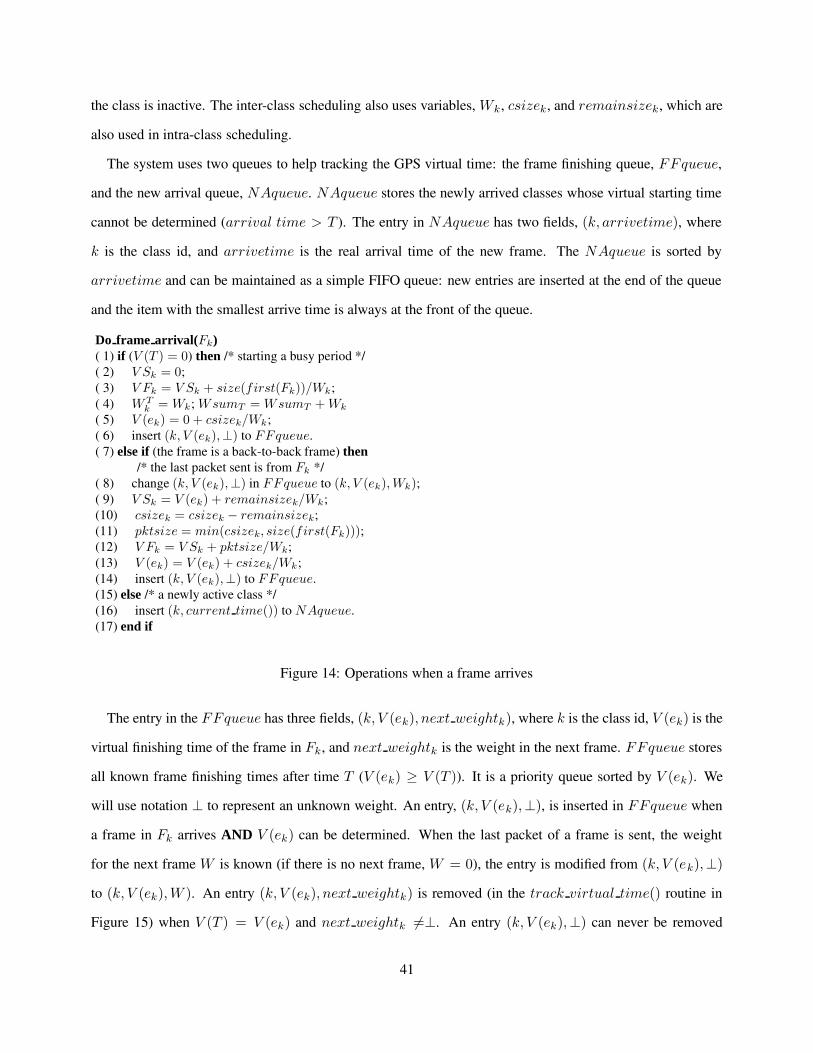
the class is inactive. The inter-class scheduling also uses variables, Wk, csizek, and remainsizek, which are

also used in intra-class scheduling.

The system uses two queues to help tracking the GPS virtual time: the frame finishing queue, FFqueue,

and the new arrival queue, NAqueue. NAqueue stores the newly arrived classes whose virtual starting time

cannot be determined (arrival time > T ). The entry in NAqueue has two fields, (k, arrivetime), where

k is the class id, and arrivetime is the real arrival time of the new frame. The NAqueue is sorted by

arrivetime and can be maintained as a simple FIFO queue: new entries are inserted at the end of the queue

and the item with the smallest arrive time is always at the front of the queue.

Do frame arrival(Fk)( 1) if (V (T ) = 0) then /* starting a busy period */( 2) V Sk = 0;( 3) V Fk = V Sk + size(first(Fk))/Wk;( 4) W T

k = Wk; WsumT = WsumT + Wk

( 5) V (ek) = 0 + csizek/Wk;( 6) insert (k, V (ek),⊥) to FFqueue.( 7) else if (the frame is a back-to-back frame) then

/* the last packet sent is from Fk */( 8) change (k, V (ek),⊥) in FFqueue to (k, V (ek), Wk);( 9) V Sk = V (ek) + remainsizek/Wk;(10) csizek = csizek − remainsizek;(11) pktsize = min(csizek, size(first(Fk)));(12) V Fk = V Sk + pktsize/Wk;(13) V (ek) = V (ek) + csizek/Wk;(14) insert (k, V (ek),⊥) to FFqueue.(15) else /* a newly active class */(16) insert (k, current time()) to NAqueue.(17) end if

Figure 14: Operations when a frame arrives

The entry in the FFqueue has three fields, (k, V (ek), next weightk), where k is the class id, V (ek) is the

virtual finishing time of the frame in Fk, and next weightk is the weight in the next frame. FFqueue stores

all known frame finishing times after time T (V (ek) ≥ V (T )). It is a priority queue sorted by V (ek). We

will use notation ⊥ to represent an unknown weight. An entry, (k, V (ek),⊥), is inserted in FFqueue when

a frame in Fk arrives AND V (ek) can be determined. When the last packet of a frame is sent, the weight

for the next frame W is known (if there is no next frame, W = 0), the entry is modified from (k, V (ek),⊥)

to (k, V (ek),W ). An entry (k, V (ek), next weightk) is removed (in the track virtual time() routine in

Figure 15) when V (T ) = V (ek) and next weightk 6=⊥. An entry (k, V (ek),⊥) can never be removed

41

(V (T ) cannot pass this time since the future weight for Fk is unknown). For such an entry, the next weightk

is always changed to a known value when the last packet is sent before it can be removed. Since a new frame

for a class is formed only after the last packet of the current frame is sent, there can be at most two entries for

each class Fk in FFqueue and the size of FFqueue is at most 2n. We assume that each class has pointers to

access their entries in FFqueue and NAqueue.

Figure 14 shows the operations when a frame arrives. If the virtual start time and the weight of a new frame

in Fk are known, variables V (ek), V Sk, V Fk can be computed based on the frame virtual start time, frame size

(csizek), remainsizek, and Wk. We will use the term frame starting sequence to denote the operations for

computing these variables and inserting (k, V (ek),⊥) to FFqueue. Lines (9) to (14) in Figure 14 constitute

a frame starting sequence. We will use the term frame finishing sequence to denote the operations to update

the next weightk field when the last packet in a frame is sent. An example of a frame finishing sequence is

shown in Line (8) in Figure 14. There are three cases in Do frame arrival(). First, when the busy period

just starts, the virtual start time of the frame is 0 and the frame starting sequence is carried out. W Tk and

WsumT are adjusted accordingly. Second, when the frame Fk is a back-to-back frame (the last packet is

from Fk), the virtual starting time of the next frame is the virtual finishing time of the last frame. In this

case, the frame finishing sequence for the old frame is carried out before the frame starting sequence for the

new frame. Last, when a new frame arrives, a new entry (k, atime = current time()) is added to the end

of the NAqueuek. Note that the timestamps for the first packet in the class are BigNUM in this case and

packets in Fk are ineligible for scheduling at this time. This class will become eligible when T = atime in

the track virtual time() routine. Since Do frame arrival() is called before track virtual time() in the

FRR scheduling module, when the arrival time of a new frame is always larger than the current T , which

was updated in the previous invocation of the FRR scheduling module.

DW 2F 2Q(), shown in Figure 15, has three tasks: (1) bookkeeping after each packet is sent (Do packetsent());

(2) updating T/V (T ) and performing the related operations (track virtual time()); and (3) selecting the

class based on the timestamps of the first packets in the classes.

There are two cases in Do packetsent(). First, when the packet sent is not the last packet in a frame, then

the timestamps, V Sk and V Fk, for the head of line packet in this class are updated. Lines (3) and (4) imply

the logic to assign the virtual finishing time of the frame as the timestamp of the last packet of the frame.

Second, the packet sent is the last packet in a frame. In this case, when the class has a back-to-back frame,

42

DW 2F 2Q()(1) Let lpkt be the last packet sent. Let lpkt be from Fk;(2) Do packetsent(lpkt,Fk);(3) track virtual time();(4) Find a class Fk whose V Sk ≤ T and V Fk is the smallest(5) return Fk.Do packetsent(lpkt, Fk)( 1) if (lpkt is not the last packet in the frame) then( 2) V Sk = V Fk;( 3) pktsize = min(csizek, size(first(Fk)));( 4) V Fk = V Sk + pktsize/Wk;( 5) else /* lpkt is the last packet in a frame */( 6) if (Fk is not backlogged) then( 7) if (remainsizek = 0) then( 8) change (k, V (ek),⊥) to (k, V (ek), 0)( 9) else(10) Wk = 1/Ck;(11) change (k, V (ek),⊥) to (k, V (ek), Wk)(12) V (ek) = V (ek) + remainsizek/Wk;(13) insert (k, V (ek), 0) to FFqueue;(14) end if(15) end if(16) end iftrack virtual time()( 1) tracking = 1;( 2) while (tracking = 1) do( 3) Let (k, V (ek), X) be the entry with the smallest V (ek) in FFqueue;( 4) Let (l, atime) be the first entry in NAqueue;( 5) vctime = V (T ) + (current time() − T )/WsumT ;( 6) vatime = V (T ) + (atime − T )/WsumT ;( 7) Let earliestv be the smallest among vctime, vatime, and V (ek).( 8) T = (earliestv − T ) ∗ WsumT + T ;( 9) V (T ) = earliestv;(10) if (earliestv = vatime) then(11) remove (l, atime) from NAqueue;(12) if (earliestv < V (el)) then(13) vstime = V (el);(14) change (l, V (el), X) to (l, V (el), Wl) ;(15) else vstime = earliestv;(16) V Sl = vstime;(17) V Fl = V Sl + size(first(Fl))/Wl;(18) V (el) = vstime + csizel/Wl;(19) insert (l, V (el),⊥) to FFqueue;(20) WsumT = WsumT + Wl;(21) W T

l = Wl;(22) end if(23) if (earliestv = V (ek)) then(24) if (X 6=⊥) then(25) WsumT = WsumT + X − W T

k ;(26) W T

k = X;(27) remove (k, V (ek), X) from FFqueue;(28) else tracking = 0;(29) end if(30) if (earliestv = vctime) tracking = 0;(31) end while

Figure 15: Inter-class scheduling

43

the case is handled in Do frame arrival(). Otherwise, the frame finishing sequence must be carried out. In

addition, if remainsizek 6= 0, there is a new frame (whose data is the partial packet) with no physical packets

to schedule. This frame needs to be taken into consideration when tracking the virtual time. A degenerated

frame starting sequence (lines (10) to (13)) is carried out.

In track virtual time(), the system tracks the virtual time, trying to bring T up-to-date. This routine

tracks every frame arrival (from NAqueue) and departure (from FFqueue) event from T to the current

time. The tracking stops either when T = current time or when V (T ) is a virtual finishing time of a

frame Fk and next weightk =⊥. Lines (3) to (7) finds the first event after T , which happens at virtual time

earliestv. Since there is no other event between V (T ) and earliestv and WsumT is known, T is updated to

the corresponding real time of earliestv (line (8)) and V (T ) = earliestv. Note that earliestv may be equal

to old V (T ) when there is a class with a finishing time V (T ) and an unknown next weightk . In this case, T

can only progress after the unknown next weightk is changed to a known weight when the last packet in that

frame is sent. If the first event is a frame arrival (earlistv = vatime), the corresponding entry is removed

from NAqueue and the frame virtual starting time is decided. The last frame for this class F l may not finish

under GPS at vatime. Thus, the virtual starting time of this frame is max(vatime, V (e l)). In this case,

the next weightk field of the entry (l, V (el), X) must be updated. After that, the frame starting sequence

is performed. When earlistv = V (ek), the first event is a frame departure. In this case, if the weight

of the next frame in Fk is unknown, the tracking stops. Otherwise, the corresponding entry in FFqueue

is removed; WsumT is adjusted; and the tracking continues. The tracking also stops when earliestv =

V (current time). In all the events, WsumT and W Tk are properly maintained.

The size of FFqueue is at most 2n and the size of FAqueue is at most n. Assuming that the priority

queue is used to implement FFqueue, the complexity of the insert and remove operations is O(lg(n)) in the

worst case. Among the routines in DW 2F 2Q(), track virtual time() has the highest complexity. In the

worst case, O(n) (size(FFqueue)+ size(NAqueue)) frame arrival and departure events must be processed

in one invocation of the FRR scheduling module. The worst case complexity for tracking the virtual time is

O(nlg(n)). Similarly, the worst case time for all Do frame arrival() calls in one invocation of the FRR

scheduling module is O(nlg(n)) since n insertions to FFqueue may need to be performed. Hence, the worst

case per packet scheduling complexity in FRR is O(nlg(n)) = O(1).

44