Fairness in Clustering withMultiple Sensitive Attributes

Savitha Sam Abraham• Deepak P†,• Sowmya S Sundaram••Indian Institute of Technology Madras, India

†Queen’s University Belfast, UKsavithas@cse.iitm.ac.in deepaksp@acm.org sowmya@cse.iitm.ac.in

ABSTRACTA clustering may be considered as fair on pre-specified sensi-tive attributes if the proportions of sensitive attribute groupsin each cluster reflect that in the dataset. In this paper, we con-sider the task of fair clustering for scenarios involving multiplemulti-valued or numeric sensitive attributes. We propose a fairclustering method, FairKM (Fair K-Means), that is inspired bythe popular K-Means clustering formulation. We outline a com-putational notion of fairness which is used along with a clustercoherence objective, to yield the FairKM clustering method. Weempirically evaluate our approach, wherein we quantify boththe quality and fairness of clusters, over real-world datasets. Ourexperimental evaluation illustrates that the clusters generated byFairKM fare significantly better on both clustering quality andfair representation of sensitive attribute groups compared to theclusters from a state-of-the-art baseline fair clustering method.

1 INTRODUCTIONClustering is the task of grouping a dataset of objects in sucha way that objects that are assigned to the same group, calleda cluster, are more similar to each other than those in othergroups/clusters. Clustering [10] is a well-studied and fundamen-tal task, arguably the most popular task in unsupervised or ex-ploratory data analytics. A pragmatic way of using clusteringwithin analytics pipelines is to consider objects within the samecluster as being indistinguishable. Customers in the same clus-ter are often sent the same promotional material in a targetedmarketing scenario in retail, whereas candidates clustered usingtheir resumes may be assigned the same shortlisting decision ina hiring scenario. Clustering provides a natural way to tackle theinfeasibility of doing manual per-object assessment or appreci-ation, especially in cases where the dataset in question encom-passes more than a few hundreds of objects. Central to clusteringis the notion of similarity which may need to be defined in atask-oriented manner. As an example, clustering to aid a taskon identifying tax defaulters may use a similarity measure thatfocuses more on the job and income related attributes, whereasthat for a health monitoring task may more appropriately focuson a very different set of attributes.

Usage of clustering algorithms in analytics pipelines for mak-ing important decisions open up possibilities of unfairness. Amongtwo high-level streams of fairness constructs, viz., individual fair-ness [8] and group fairness [12], we focus on the latter. Groupfairness considers fairness from the perspective of sensitive at-tributes such as gender and ethnicity and groups defined on the

© 2020 Copyright held by the owner/author(s). Published in Proceedings of the23rd International Conference on Extending Database Technology (EDBT), March30-April 2, 2020, ISBN 978-3-89318-083-7 on OpenProceedings.org.Distribution of this paper is permitted under the terms of the Creative Commonslicense CC-by-nc-nd 4.0.

basis of such sensitive attributes. Consider a clustering algo-rithm that targets to group records of individuals to clusters; itis possible and likely that certain clusters have highly skeweddistributions when profiled against particular sensitive attributes.As an example, clustering a dataset with broad representationacross gender groups based on exam scores could lead to clustersthat are highly gender-homogeneous due to statistical correla-tions1; this would happen even if the gender attribute were notexplicitly considered within the clustering, since such informa-tion could be held implicitly across one or more other attributes.Choosing a cluster with a high gender or ethnic skew for positive(e.g., interview shortlisting) or negative (e.g., higher scrutiny orchecks) action entails differentiated impact across gender andethnic groups. This could also lead to reinforcement of societalstereotypes. For example, consistently choosing individuals fromparticular ethnic groups for pro-active surveillance could leadto higher reporting of violations from such ethnic groups sinceenhanced surveillance translates to higher crime visibility, re-sulting in higher reporting rates. This reporting skew resultsthus manifests as a data skew which provides opportunities forfuture invocations of the same analytics to exhibit higher eth-nic asymmetry. In modern decision making scenarios within aliberal and democratic society, we need to account for a plu-rality of sensitive attributes within analytics pipelines to avoidcausing (unintended) discrimination; these could include gen-der, race, religion, relationship status and country of origin ingeneric decision-making scenarios, and could potentially includeattributes such as age and income in more specific ones. Therehas been much recent interest in the topic of fair clustering [1, 6].

Our Contribution. In this paper, we consider the task of fairclustering in the presence of multiple sensitive attributes. Aswill be outlined in a later section, this is a direction that hasreceived less attention amidst existing work on fair clusteringthat has been designed for scenarios involving a single binarysensitive attribute [3, 6, 14, 17], single multi-valued/categoricalsensitive attribute [1, 20–22], or multiple overlapping groups [4].We propose a clustering formulation and algorithm to embedgroup fairness in clustering that incorporates multiple sensitiveattributes that may include numeric, binary or multi-valued (i.e.,categorical) sensitive ones. Through an empirical evaluation overmultiple datasets, we illustrate the empirical effectiveness of ourapproach in generating clusters with fairer representations ofsensitive groups, while preserving cluster meaningfulness.

2 RELATEDWORKFairness in machine learning has received significant attentionover the last few years. Our work contributes to the area offair methods for unsupervised learning tasks. We now brieflysurvey the area of fairness in unsupervised learning, with a focus

1https://www.compassprep.com/new-sat-has-disadvantaged-female-testers/

arX

iv:1

910.

0511

3v2

[cs

.LG

] 2

4 Ja

n 20

20

on clustering, our task of interest. We interchangeably refer togroups defined on sensitive attributes (e.g., ethnic groups, gendergroups etc.) as protected classes for consistency with terminologyin some referenced papers. Towards developing a systematicsummary, we categorize prior work into three types dependingon whether the fairness modelling appears as a (i) pre-processingstep, (ii) during the task of clustering, or (iii) as a post-processingstep after clustering. These yield the three technique families.

2.1 Space Transformation ApproachesThe family of fairness pre-processing techniques work by firstrepresenting the data points in a ‘fair’ space followed by applyingany existing clustering algorithm upon them. This is the largestfamily of techniques, and most approaches in this family seek toachieve theoretical guarantees on representational fairness. Thisfamily includes one of the first works in this area of fair cluster-ing [6]. The work proposes a fair variant of classical clusteringfor scenarios involving a single sensitive attribute that can takebinary values. Let each object be colored either x or y dependingon its value for the binary sensitive attribute. [6] defines fair-ness in terms of balance of a cluster, which ismin{#x/#y, #y/#x}.They go on and outline the concept of (b, r )-fairlet decomposition,where the points in the dataset are grouped into small clusterscalled fairlets, such that each fairlet would have a balance of b/r ,where b < r . The clustering is then performed on these fairlets.The fairness guarantees that are provided by the clustering isbased on the balance in the underlying fairlets. Fairlet decom-position turns out to be NP-hard, for which an approximationalgorithm is provided. Later, [3] proposed a faster fairlet decom-position algorithm offering significant speedups. The work in[20] extends the fairlet idea toK-means for scenarios with a singlemulti-valued sensitive attribute. They define fair-coresets whichare smaller subsets of the original dataset, such that solving fairclustering over this subset also results in giving an approximatesolution for the entire dataset.

Another set of fair space transformation approaches buildupon methods for dimensionality reduction and representationlearning. A recent such work [2] considers the bias in the dataset(that is, representational skew) as a form of noise and uses spectralde-noising techniques to project the original points in the datasetto a new fair projected space. [17] describes a fair version of PCA(Principal Component Analysis) for data with a single binarysensitive attribute. A representation learning method may bedefined as fair if the information about the sensitive attributescannot be inferred from the learnt representations. The methoduses convex optimization formulations to embed fairness withinPCA. The fairness is specified in terms of failure of the classifiersin predicting the sensitive class of the dimensionality-reduceddata points obtained from fair PCA. The method is fairer if thedata points are less distinguishable with respect to their valuesof the sensitive attribute in this lower dimension space. Anotherwork that projects the original data points into a fair space is theone described in [21]. This method, which is for cases involvinga single multi-valued sensitive attribute, defines a clustering tobe fair when there is an equal number of data points of eachprotected class in each cluster. They define the concept of fairoids(short for fair centroids) which are formed by grouping togetherall points belonging to the same protected class. The task isthen to learn a latent representation of the data points suchthat the cluster centroids obtained after clustering on this latentrepresentation are equi-distant from every fairoid.

2.2 Fairness Modelling within OptimizationMethods in this family incorporate the fairness constraints intothe clustering step, most usually within the objective functionthat the clustering method seeks to optimize for. It may be notedthat the method we propose in this paper, FairKM, also belongs tothis family. Approaches within this family define a clustering tobe fair if the proportional representation of the protected class ina cluster reflects that in the dataset. One of the techniques [14] de-scribes a fair variant of spectral clustering where a linear fairnessconstraint is incorporated into the original ratio-cutminimizationobjective of spectral clustering. Another recent technique [22],the method that comes closest to ours in construction, modifiesK-means clustering to add a fairness loss term. The fairness lossis computed as the KL-divergence between the probability dis-tribution across the different values for the sensitive attributein a cluster, and the corresponding distribution for the wholedataset. This method is designed for a single multi-valued sensi-tive attribute and does not generalize to multiple such sensitiveattributes. Being closest to our proposed method in spirit, we usethis method as our primary baseline, in the experiments.

In contrast to the above, another recent work [5] outlines a dif-ferent notion of fairness, one that is independent of (and agnosticto) sensitive attributes. They define fairness as proportionalitywrt spatial distributions, to mean that any (n/k) points can formtheir own cluster if there exists another center that is closer toeach of these (n/k) points. This proportionality constraint is in-corporated into the objective function of k-median clusteringand is optimized to find a clustering that satisfies this constraint.

2.3 Cluster Perturbation TechniquesIn this third family of techniques, vanilla clustering is first appliedon the original set of data points, after which the generatedclusters are perturbed to improve fairness of the solution. In[4], fairness is defined in terms of a lower and upper bound onthe representation of a protected class in a cluster. This methodis for cases with multiple binary sensitive attributes, referredto as overlapping groups in the paper. The k-centers generatedfrom vanilla clustering on the data points are used to performa fair partial assignment between points and the centers. Thefair partial assignment is formulated as a linear program withconstraints that ensures that the sum of the weights associatedwith a point’s partial assignments is one, and, the representationof a protected class in a cluster is within the specified upperand lower bounds. The partial assignments are then converted tointegral assignments by framing it as another linear programmingproblem. [1] also uses a similar idea, but it just enforces an upperbound, consequently preventing over-representation of specificgroups in a cluster. The work described in [13] proposes a simpleapproximation algorithm for k-center clustering under a fairnessconstraint, for scenarios with a single multi-valued sensitiveattribute. The method targets to generate a fair summary of alarge set of data points, such that the summary is a representativesubset of the original dataset. For example, if the original datasethas a 70:30 male:female distribution, then a fair summary shouldalso have the same distribution.

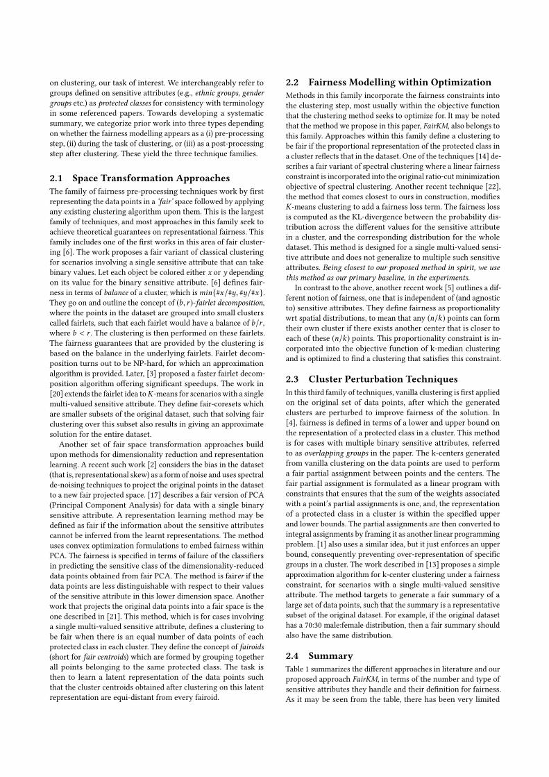
2.4 SummaryTable 1 summarizes the different approaches in literature and ourproposed approach FairKM, in terms of the number and type ofsensitive attributes they handle and their definition for fairness.As it may be seen from the table, there has been very limited

Paper Number Type Fairness Definition[6],[3],[2] Single Binary Preserve proportional representation of protected classes within clusters.[20] Single Multi-valued Preserve proportional representation of protected classes within clusters.[17] Single Binary The accuracy of the classifier predicting the protected class of a data point should be within

a specified bound.[21] Single Multi-valued Each cluster should have an equal number of data points from each protected class.[4] Multiple Binary The proportional representation of a protected class in a cluster should be within the specified

lower and upper bounds.[1] Single Multi-valued The proportional representation of a protected class in a cluster should not go beyond a

specified upper bound.[13] Single Multi-valued The clustering should produce pre-specified number of cluster centers belonging to each

specific protected class.[14], [22] Single Multi-valued Preserve proportional representation of protected classes within clusters.[5] - - There are no set of (n/k) points such that there exists another center that is closer to each of

these (n/k) points.[18] Single Multi-valued Each cluster should have atleast a pre-specified number of points of a protected class.FairKM Multiple Multi-valued/ Preserve proportional representation of protected classes within clusters.

Numeric as its representation in the whole dataset.Table 1: Fair Unsupervised ML Methods indicating the Number and Type of Sensitive Attributes they are designed for.

exploration into methods that admit multiple multi-valued (akacategorical or multi-state) sensitive attributes, the space thatFairKM falls in. While multiple multi-valued attributes can betreated as together forming a giant multi-valued attribute takingvalues that are combinations of the component attributes, thisresults in a large number of very fine-grained groupings. Thesemake it infeasible to both (i) impose fairness constraints over,and (ii) ensure parity in treatment of different sensitive attributesindependent of the differences in the number of values they take.Considering the fact that real-life scenarios routinely presentwith multiple sensitive attributes, FairKM, we believe addressesan important line of inquiry in the backdrop of the literature. Wewill empirically evaluate FairKM against [22], the latter comingfrom the same technique family and having similar construction.

3 PROBLEM DEFINITIONLet X = {. . . ,X , . . .} be a dataset of records defined over twosets of attributesN and S.N stands for the set of attributes thatare relevant to the task of interest, and thus may be regardednon-sensitive. As examples, this may comprise experience andskills in the case of screening applicants for a job application,and attributes from medical wearables’ data to inform decisionmaking for pro-active screening. S stands for the set of sensitiveattributes, which would typically include attributes such as thoseidentifying gender, race, religion, relationship status in a citizendatabase and any other sensitive attribute over which fairnessis to be ensured. In other scenarios such as NLP for education,representational fairness may be sought over attributes such astypes of problems in a word problem database; this forms one ofthe scenarios in our empirical evaluation.

The (vanilla) clustering objective would be to group X intoclusters such that it maximizes intra-cluster similarity and mini-mizes inter-cluster similarity, similarity gauged using the task-relevant attributes inN . Within a fair clustering, we would addi-tionally like the output clusters to be fair on attributes in S. Anatural way to operationalize fairness within a clustering thatcovers all objects in X would be to ensure that the distribution ofgroups defined on sensitive attributes within each cluster approx-imates the distribution across the dataset; this correlates with the

well-explored notion of statistical parity [8] in fair supervisedlearning. For example, suppose the sex ratio inX is 1:1; we wouldideally like each cluster in the clustering output to report a sexratio of 1:1, or very close to it. In short, we would like a fairclustering to produce clusters, each of which are both:• coherent when measured on the attributes in N , and• approximate the dataset distribution when measured on theattributes in S.It may be noted that simply hiding the S attributes from the

clustering algorithm does not suffice. A gender blind cluster-ing algorithm may still produce clusters that are highly gender-homogeneous, since some attributes inN could implicitly encodegender information. Indeed, we would like a fair clustering tosurpass S-blind clustering by significant margins on fairness.

4 FAIRKM: OUR METHODWe now describe our proposed technique for fair clustering, code-named FairKM, short for Fair K-Means, indicating that it drawsinspiration from the classical K-Means clustering algorithm [9,16]. FairKM incorporates a novel fairness loss term that nudgesthe clustering towards fairness on attributes in S. The FairKMobjective function is as follows:

O =∑C ∈C

∑X ∈C

distN(X ,C)︸ ︷︷ ︸K-Means Term over attributes in N

+λ deviationS(C,X)︸ ︷︷ ︸Fairness Term over attributes in S

(1)

As indicated, the objective function comprises two compo-nents; the first is the usual K-Means loss for the clustering C,distN(X ,C) computing the distance between X and prototypeof cluster C , distance computed only over attributes in N . Thesecond is a fairness loss term we introduce, which is computedover attributes in S. λ is a parameter that may be used to balancethe relative strength of the two terms. As in K-Means, this lossis computed over a given clustering; the task is thus to identify

a clustering that minimizes O as much as possible. We now de-scribe the details of the second term, and the intuitions behindits construction.

4.1 The Fairness Term in FairKMWhile the K-Means term in the FairKM objective tries to ensurethat the output clusters are coherent in theN attributes, the fair-ness term performs the complementary function of ensuring thatthe clusters manifest fair distributions of groups defined by sensi-tive attributes in S. We outline the motivation and constructionof the fairness term herein.Attribute-Specific Deviation for a Cluster: Consider a singlesensitive attribute S (e.g., gender) among the set of sensitiveattributesS. For each data objectX , S may take on one value froma set of permissible values. Let s be one such value (e.g., female, forthe choice of S as gender). For an ideally fair clusterC , one wouldexpect that the fractional representation of s inC - the fraction ofobjects inC that take the value s for S - to be close to the fractionalrepresentation of s in X. With our intent of generating clustersthat are as fair as possible, we seek to generate clusterings suchthat the deviation between the fractional representations of s inC and X are minimized for each cluster C . For a given cluster Cand a choice of value s for S , we model the deviation as simplythe square of the absolute differences between the fractionalrepresentations in C and X:

DSC (s) =

(|{X |X ∈ C ∧ X .S = s}|

|C | − |{X |X ∈ X ∧ X .S = s}||X|

)2(2)

The deviation, when aggregated over all values of S , yields:

DSC =

{∑s ∈Values(S ) D

SC (s) |C | , 0

0 |C | = 0(3)

The above aggregation accounts for the fact that DSC (s) is

undefined when C is an empty cluster.Domain Cardinality Normalization: Different sensitive at-tributes may have different numbers of permissible values (ordomain cardinalities). For example, race and gender attributestypically take on much fewer values than country of origin. Thoseattributes with larger domains are likely to yield largerDS

C scoresbecause, (i) the deviations are harder to control within (small)clusters given the higher likely scatter, and (ii) there are largernumbers of DS

C (s) terms that add up to DSC . In order to ensure

that attributes with larger domains do not dominate the fair-ness term, we normalize the deviation by the number of differ-ent values taken by an attribute, yielding NDS

C , a normalizedattribute-specific deviation:

NDSC =

DSC

|Values(S)| (4)

This is then summed up over all attributes in S to yield asingle term for each cluster:

NDC =∑S ∈S

NDSC (5)

Cluster Weighting: Observe that NDC deviation loss wouldtend towards 0.0 for very large clusters, since they are obvi-ously likely to reflect dataset-level distributions better; further,an empty cluster would also have NDS

C = 0 by definition. Consid-ering the above, a clustering loss term modelled as a simple sum

over its clusters,( ∑

C ∈C NDC)or a cardinality weighted sum,( ∑

C ∈C |C | × NDC), can both be driven towards 0.0 by keeping

a lot of clusters empty, and distributing the dataset objects acrossvery few clusters; the boundary case would be a single non-emptycluster. Indeed, this propensity towards the boundary conditionis kept in check by the K-Means term; however, we would likeour fairness term to drive the search towards more reasonable fairclustering configurations in lieu of simply reflecting a propensitytowards highly skewed clustering configurations.

Towards achieving this, we weight each cluster’s deviation bythe square of it’s fractional cardinality of the dataset. This leadsto an overall loss term as follows:∑

C ∈C

(|C ||X|

)2× NDC (6)

The squared term in the weighting enlarges the NDC terms oflarger clusters much more than smaller ones, making it unprof-itable to create large clusters; this compensates for the propensitytowards skewed clusters as embodied in the loss construction.Overall Loss: The overall fairness loss term is thus:

deviationS(C,X) =∑C ∈C

(|C ||X|

)2×

∑S ∈S

∑s ∈Values(S )

(FrSC (s) − FrSX(s)

)2|Values(S)| (7)

where FrSC (s) and FrSX(s) are shorthands for the fractionalrepresentation of S = s objects in C and X respectively.

4.2 The Optimization ApproachHaving defined the objective function, we now outline the opti-mization approach. It is easy to observe that there are three setsof parameters, the clustering assignments for each data object inX, the cluster prototypes that are used in the first term of the ob-jective function, and the fractional representations, i.e., FrSC (s)s,used in the fairness term. Unlike K-Means, given the more com-plex construction, it is harder to form a closed-form solutionfor the cluster assignments. Thus, from a given estimate of allthree sets of parameters, we step over each data object X ∈ X inround-robin fashion, updating its cluster assignment, and makingconsequent changes in cluster prototypes and fractional repre-sentations. One set of round-robin updates forms an iteration,with multiple such iterations performed until convergence oruntil a maximum threshold of iterations is reached.

4.2.1 Cluster Assignment Updates. At λ = 0, FairKM defaultsto K-Means where the cluster assignments are determined onlyby proximity to the cluster prototype (over attributes in N ). Athigher values of λ, FairKM cluster assignments are increasinglyswayed by considerations of representational fairness of S at-tributes within clusters.

It may be noted that the cluster assignments are used in boththe terms of the FairKM objective, in different ways. This makes aclosed form estimation of cluster assignments harder to arrive at.This leads us to a round-robin approach of determining clusterassignments. When each X is considered, the cluster prototypesas well as the current cluster assignments of all other objects, i.e.X − {X }, are kept unchanged. The cluster assignment for X isthen estimated as:

Cluster (X ) = argminC

OC+(X ∈C) (8)

For the candidate object X , we evaluate the value of the ob-jective function by changing X ’s cluster membership from thepresent one to each cluster, C + (X ∈ C) indicating a correspond-ing change in the clustering configuration retaining all otherobjects’ present cluster assignments. X is then assigned to thecluster for which the minimum value of O is achieved. Whilethis may look as a simple step, implementing it naively is compu-tationally expensive. However, easy optimizations are possiblewhen one observes the dynamics of the change and how it op-erates across the two terms. We now outline a simple way ofaffecting the cluster assignment decision. First, let X ’s currentcluster assignment be C ′; the cluster assignment step can beequivalently written as:

Cluster (X ) = argminC

δ (O)X ∈C ′→X ∈C (9)

where δO indicates the change in O when the respective clus-ter assignment change is carried out. This can be expanded intothe changes in the two terms in the objective function as follows:

δ (O)X ∈C ′→X ∈C =

δ (K-Means term)X ∈C ′→X ∈C+λ×δ (deviation term)X ∈C ′→X ∈C(10)

We now detail the changes in the respective terms separately.Change in K-Means Term:We now outline the change in theK-Means term bymovingX fromC ′ toC . As may be obvious, thisdepends only on attributes inN . We model the cluster prototypesas simply the average of the objects within the cluster. The changein the K-Means term is the sum of (i) the change in the K-Meansterm corresponding to C ′ brought about by the exclusion of Xfrom it, and (ii) the change in the K-Means term correspondingto C brought about by the inclusion of X within it. We discussthem below.

Consider a single numeric attribute N ∈ N , for simplicity.Through excludingX fromC ′, the N attribute value of the clusterprototype of C ′ undergoes the following change:

C ′.N →[(C ′.N − X .N

|C ′ |

)× |C ′ |

|C ′ − 1|

](11)

where C ′ is overloaded to refer to the cluster and the clusterprototype (to avoid clutter), all values referring to those priorto exclusion of X . The term after the → stands for the N at-tribute value for the new cluster prototype. As indicated, it iscomputed by the removal of the contribution from X from thecluster prototype, followed by re-normalization, now that C ′ hasone fewer object within it. The change in the K-Means term forN corresponding to C ′ is then as follows:

δXoutKM(C ′,N ) =( ∑X ′∈C ′,X ′,X

(X ′.N − New(C ′.N ))2)−[( ∑

X ′∈C ′,X ′,X(X ′.N −C ′.N )2

)+ (X .N −C ′.N )2

](12)

where New(C ′.N ) is the new estimate of C ′.N as outlined inEq. 11. The first term corresponds to the K-Means loss in thenew configuration (after exclusion of X ), whereas the sum of thesecond and third terms correspond to that prior to exclusion ofX . Analogous to the above, the new centroid computation for Cand the change in the K-Means terms are outlined below:

C .N →[(C .N × |C |

|C + 1|

)+

X .N

C + 1

](13)

δXinKM(C,N ) =[( ∑

X ′∈C,X ′,X(X ′.N − New(C .N ))2

)+

(X .N − New(C .N ))2]−( ∑X ′∈C,X ′,X

(X ′.N −C .N )2)

(14)

It may be noticed that the computation of the changes aboveonly involve X and other objects in C and C ′. In particular, theother clusters and their objects do not come into play. So far, wehave computed the changes for only one attribute N . The overallchange in the K-Means term is simply the sum of these changesacross all attributes in N .

δ (K-Means term)X ∈C ′→X ∈C =∑N ∈N

(δXoutKM(C ′,N ) + δXinKM(C,N )

)(15)

Change in Fairness Term:We now outline the construction ofthe change in the fairness term. As earlier, we start by consideringa single clusterC∗, a single attribute S , and a single value s withinit. The fairness term from Eq. 7 can be written as follows:

dev(C∗, S = s) =C∗2 ×

((C∗s

C∗

)2+

(XsX

)2− 2C

∗s XsC∗ X

)X2 × |Values(S)|

(16)

where each set (C∗ and X) is overloaded to represent bothitself and its cardinality (to avoid notation clutter), and theirsuffixed versions (C∗

s and Xs ) are used to refer to their subsetscontaining their objects which take the value S = s . The aboveequation follows from the observation that FrSC∗ (s) =

C∗S

C∗ andanalogously for X. When an object changes clusters from C ′ toC , there is a change in the terms associated with both clusters, asin the previous case. The change in the origin cluster C ′ worksout to be the follows:

δXoutdev(C′, S = s) = 1

X2 × |Values(S)|×[(XsX

)2(1 − 2C ′)+

I(X .S = s)(1 − 2C ′s ) − 2

(XsX

) (I(X .S = s)(1 −C ′) −C ′

s

)](17)

where I(.) is an indicator function, and C ′ and C ′s denote the

cardinalities before X is taken out of C ′. We omit the deriva-tion for space constraints. Intuitively, to nudge clusters towardsfairness, we would like to incentivize removal of objects withS = s from C ′ when C ′ is overpopulated with such objects (i.e.,C ′s is high). This is evident in the −(C ′

s × I(X .S = s)) component;when C ′

s is high, removal of an object with S = s entails a biggerreduction in the objective. The analogous change in the targetcluster C , is as follows:

δXindev(C, S = s) =1

X2 × |Values(S)|×[(XsX

)2(1 + 2C)+

I(X .S = s)(1 + 2Cs ) − 2(XsX

) (I(X .S = s)(1 +C) +Cs

)](18)

where C and Cs denote the cardinalities before X is insertedintoC . Given that we are insertingX intoC , the fairness intuitionsuggests that we should disincentivize addition of objects with swhen C already has too many of such objects. This is reflectedin the (Cs × I(X .S = s)) term; notice that this is exactly the sameterm as in the earlier case, but with a different sign.

Thus, the overall fairness term change is as follows:

δ (deviation term)X ∈C ′→X ∈C =∑S ∈S

∑s ∈Values(S )

(δXoutdev(C

′, S = s) + δXindev(C, S = s))(19)

This completes all the steps required for Eq. 9. Based on thechange in the cluster assignment, the cluster prototypes andfractional representations are to be updated.

4.2.2 Cluster Prototype Updates. Once a new cluster has beenfinalized for X , the origin and target cluster prototypes are up-dated according to Eq. 12 and Eq. 14 respectively.

4.2.3 Fractional Representation Updates. The FrSC ′(s)s andFrSC (s)s need to be updated to reflect the change in the clusterassignment of X . These are straightforward and given as follows:

∀S∀s ∈ Values(S), FrSC ′(s) ={C ′

s−1C ′−1 if X .S = sC ′s

C ′−1 if X .S , s(20)

∀S∀s ∈ Values(S), FrSC (s) ={Cs+1C+1 if X .S = sCsC ′+1 if X .S , s

(21)

where the C , C ′, Cs and C ′s values above are cardinalities of

the respective sets prior to the update to X ’s cluster assignment.

Alg. 1 FairKM

Input. Dataset X, attribute sets S and N , number of clusters kHyper-parameters: Fairness Weighting λOutput. Clustering C1. Initialize k clusters randomly2. Set cluster prototypes as Cluster Centroids3.while(not yet converдed and max . iterations not reached)4. ∀X ∈ X,5. Set Cluster(X) using Eq. 9 (and Eq. 10 through Eq. 19)6. Update cluster prototypes as outlined in Sec 4.2.27. Re-estimate the FrSC (s) using Eq. 20 and Eq. 218. Return the current clustering assignments as C

4.3 FairKM AlgorithmHaving outlined the various steps, the FairKM algorithm can nowbe summarized in Algorithm 1. The method starts with a ran-dom initialization of clusterings (Step 1) and proceeds iteratively.Within each iteration, each object is considered in round-robinfashion, executing three steps in sequence: (i) updating the clus-ter assignment of X (Step 5), (ii) updating the cluster prototypesto reflect the change in cluster assignment of X (Step 6), and (iii)updating the fractional representations correspondingly (Step7). The significant difference in construction from K-Means isdue to the inter-dependency in cluster assignments; the clusterassignment for X depends on the current cluster assignments forall other objects X − {X }, due to the construction of the FairKM

objective as reflected in the update steps. The updates proceedas long as the clustering assignments have not converged or apre-specified maximum number of iterations have not reached.

4.3.1 Complexity: The time complexity of FairKM is domi-nated by the cluster assignment updates. Within each iteration,for each X (|X| of them) and each cluster it could be re-assignedto (k of them), the deviation needs to be computed for both the(i) K-Means term, and the (ii) fairness term. First, consideringthe K-Means term, it may be noted that each other object in Xwould come into play once, either as a member of X ’s currentcluster (in Eq. 12) or as a member of a potential cluster to whichX may be assigned (in Eq. 14). This yields an overall complex-ity of each K-Means deviation computation being in O(|X||N |).Second, considering the fairness deviation computation, it maybe seen as a simple computation (Eq. 17 and 18) that can be com-pleted in constant time. This computation needs to be performedfor each attribute in S and each value of the attribute (considerm as the maximum number of values across attributes in S),yielding a total complexity of O(|S|m) for each fairness updatecomputation. With the updates needing to be computed for eachnew candidate cluster, the overall complexity of Step 5 wouldbe O(|X||N |k + |S|mk). Step 6 is in O(|X||N |) whereas Step 7 issimply in O(|S|m). With the above steps having to be performedfor each X and for each iteration, the overall FairKM complex-ity works out to be in O(|X|2 |N |kl + |X||S|mkl) where l is thenumber of iterations. While the quadratic dependency on thedataset size makes FairKM much slower than simple K-Means(which is linear on dataset size), FairKM compares very favorablyagainst other fair clustering methods (e.g., exact fairlet decom-position [6] is NP-hard, and even the proposed approximation issuper-quadratic) which are computationally intensive.

4.4 FairKM ExtensionsWe outline two extensions to the basic FairKM outlined earlierwhich was intended towards handling numeric non-sensitiveattributes and multi-valued sensitive attributes.

4.4.1 Extension to Numeric Sensitive Attributes. FairKM is eas-ily adaptable to numeric sensitive attributes (e.g., age for caseswhere that is appropriate). If all attributes in S are numeric, thefairness loss term in Eq. 7 would be written out as:

deviationS(C,X) =∑C ∈C

(|C ||X|

)2×

∑S ∈S

(C .S − X.S)2 (22)

where C .S and X.S indicate the average value of the numericattribute S across objects in C and X respectively. When thereare a mix of multi-valued and numeric attributes, the inner termwould take the form of Eq. 7 and Eq. 22 for multi-valued and nu-meric attributes respectively. These entail corresponding changesto the update equations which we do not describe here for brevity.

4.4.2 Extension to allow Sensitive Attribute Weighting. In cer-tain scenarios, some sensitive attributes may need to be consid-ered more important than others. This may be due to historicalreasons based on a legacy of documented high discriminationon certain attributes, or due to visibility reasons where discrimi-nation on certain attributes (e.g., gender, race and sexual orienta-tion) being more visible than others (e.g., country of origin). TheFairKM framework could easily be extended to allow for differen-tial attribute-specific weighting by changing the deviation termto be as follows:

deviationS(C,X) =∑C ∈C

(|C ||X|

)2×

∑S ∈S

wS ×∑s ∈Values(S )

(FrSC (s) − FrSX(s)

)2|Values(S)|

(23)

Attributes that are more important for fairness considerationscan then be assigned a higher weight, i.e.wS , which would leadto their loss being amplified, thus incentivizing FairKM to focusmore on them for fairness, consequently leading to a higher rep-resentational fairness over them, within the clusters in the output.ThewS terms would then also affect the update equations.

5 EXPERIMENTAL STUDYWe now detail our experimental study to gauge and quantifythe effectiveness of FairKM in delivering good quality and fairclusterings against state-of-the-art baselines. We first outline thedatasets in our experimental setup, followed by a description ofthe evaluation measures and baselines. This is then followed byour results and an analysis of the results.

5.1 DatasetsWe use two real-world datasets in our empirical study. Thedatasets are chosen to cover very different domains, attributesand dataset sizes, to draw generalizable insights from the study.First, we use the popular Adult dataset from UCI repository [7];this dataset is sometimes referenced as the Census Income datasetand contains information from the 1994 US Census. The datasethas 32561 instances, each instance represented using 13 attributes.Among the 13 attributes, 5 are chosen to form the set of sensi-tive attributes, S. These are {marital status , relationship status ,race , дender , native country}. The number of values taken byeach of the sensitive attributes are shown in Table 3. The setof non-sensitive attributes, N , pertain to age, work class (2 at-tributes), education (2 attributes), occupation, fiscal information(2 attributes) and number of working hours. The dataset has beenwidely used for predicting income as belonging to one of > 50k$or <= 50k$. We first undersample the dataset to ensure parityacross this income class attribute that we do not use in the cluster-ing process. The total number of instances after undersamplingis 15682. Second, we use a dataset2 of 161 word problems fromthe domain of kinematics. Kinematics is the study of motionwithout considering the cause of motion. The problems in thisdataset is categorized into various types as indicated in Table 2.The complexity of a word problem typically depends on the type.For example, Type 1 problems are easier to solve (in terms of theequations required) compared to Type 5 problems. Table 4 showsthe number of problems of each of the above types in the dataset.Given such a dataset of word problems from kinematics domain,we are interested in the task of clustering the word problemssuch that the proportional representation of problems of a par-ticular type in a cluster reflects its representation in the entiredataset. In the application scenario of automatic construction ofmultiple questionnaires (one from each cluster) from a questionbank, the fair clustering task corresponds to ensuring that eachquestionnaire contains a reasonable mix of problem types. Thisensures that there is minimal asymmetry between the differentquestionnaires generated by a clustering, in terms of overall hard-ness. For the fair clustering formulation, thus, the problem types2https://github.com/savithaabraham/Datasets

form the set of 5 sensitive binary attributes, S. The lexical rep-resentation of each word problem, as a 100 dimensional vectorusing Doc2Vec models [15], forms the set of numeric attributesin N . Given our fairness consideration, we consider achieving afair proportion of word problem types within each cluster thatreflects their proportion across the dataset.

It may be noted that the Adult and Kinematics datasets comefrom different domains (Census and Word Problems/NLP respec-tively), have different sizes of non-sensitive attribute sets (8 and100 attributes in N respectively), different kinds of sensitiveattribute sets (multi-valued and binary respectively) and havewidely varying sizes (15k and 161 respectively). An empiricalevaluation over such widely varying datasets, we expect, wouldinspire confidence in the generalizability of empirical results.

5.2 EvaluationHaving defined the task of fair clustering in Section 3, it followsthat a fair clustering algorithmwould be expected to performwellon two sets of evaluation metrics, those that relate to clusteringquality over N and those that relate to fairness over S. We nowoutline such evaluation measures below, in separate subsections.

5.2.1 Clustering Quality. These measure how well the clus-tering fares in generating clusters that are coherent on attributesin N , and do not depend on attributes in S. These could include:

• Silhouette Score (SH): Silhouette [19] measures the separated-ness of clusters, and quantifies a clustering with a score in[−1,+1], higher values indicating well-separated clusters.

• Clustering Objective (CO): Clustering objective functions suchas those employed by K-Means [16] measure how much ob-servations deviate from the centroids of the clusters they areassigned to, where lower values indicate coherent clusters. Inparticular, the K-Means objective function is:∑

C ∈C

∑X ∈C

distN(X ,C) (24)

where C stands for both a cluster in the clustering C as wellas the prototype object for the cluster, and distN(., .) is thedistance measure computed over attributes in N .

• Deviation from S-blind Clusterings: S-blind clusterings maybe thought of achieving the best possible clusters for the taskwhen no fairness considerations are imposed. Thus, amongtwo clusterings of similar fairness, that with lower deviationfrom S-blind clusterings may be considered desirable. A fairclustering can be compared with a S-blind clustering usingthe following two measures:– Centroid-based Deviation (DevC): Consider each clusteringto be represented as a set of cluster centroids, one for eachcluster within the clustering. The sum of pair-wise dot-products between centroid pairs, each pair constructed usingone centroid from the fair clustering and one from the S-blind clustering, would be a measure of deviation betweenthe clusterings. Such measures have been used in generatingdisparate clusterings [11].

– Object pair-wise Deviation (DevO): Consider each pair ofobjects from X, and one clustering (either of S-blind andfair); the objects may belong to either the same cluster orto different clusters. The fraction of object pairs from Xwhere the same/different verdicts from the two clusteringsdisagree provide an intuitive measure of deviation betweenclusterings.

Type Description1:Horizontal Motion The object involved is in a horizontal straight line motion.2:Vertical motion with an initial velocity The object is thrown straight up or down with a velocity.3:Free fall The object is in a free fall.4:Horizontally projected The object is projected horizontally from a height.5:Two-dimensional The body is projected with a velocity at an angle to the horizontal.

Table 2: Kinematics Word Problem Types

Attribute No. of valuesMarital status 7Relationship status 6Race 5Gender 2Native country 41

Table 3: Adult Dataset: Number of possible values for eachsensitive attribute

Type Count1 - Horizontal motion 602 - Vertical motion with an initial velocity 363 - Free fall 154 - Horizontally projected 315 - Two-dimensional 19

Table 4: Kinematics Dataset: #Problems of each Type

5.2.2 Fairness. These measure the fairness of the clusteringoutput from the (fair) clustering algorithm. Analogous to cluster-ing quality measures that depend only on N , the fairness mea-sures we outline below depend only on S and are independentof N . As outlined earlier, we quantify unfairness as the extentof deviation between representations of groups defined usingattributes in S in the dataset and each cluster in the clusteringoutput. Consider a multi-valued attribute S ∈ S, which can takeon t values. The normalized distribution of presence of each ofthe t values in X yields a t-length probability distribution vectorXS . A similar probability distribution can then be computed foreach cluster C in the clustering C, denoted CS . Different ways ofmeasuring the cluster-specific deviations {. . . ,dev(CS ,XS ), . . .}and aggregating them to a single number yield different quantifi-cations of fairness, as below:• Average Euclidean (AE): This measures the average of cluster-level deviations, deviations quantified using euclidean distancebetween representation vectors (i.e., XS and CS s). Since clus-ters may not always be of uniform sizes, we use a cluster-cardinality weighted average.

AES =

∑C ∈C |C | × ED(CS ,XS )∑

C ∈C |C | (25)

where ED(., .) denotes the euclidean distance.• Average Wasserstein (AW): In this measure, the deviation iscomputed using Wasserstein distance in lieu of Euclidean, asused in [21], with other aspects remaining the same as above.

• Max Euclidean (ME): Often, just optimizing for average fair-ness across clusters is not enough since there could be a veryskewed (small) cluster, whose effect may be obscured by other

clusters. It is often the case that one or few clusters get pickedfrom a clustering to be actioned upon. Thus, the maximumskew is of interest as an indicative upper bound on the un-fairness the clustering could cause if any one of its clusters ischosen for further action.

• Max Wasserstein (MW): This uses Wasserstein instead of Eu-clidean, using the same formulation as Max Euclidean.

When there are multiple attributes in S, as is often the case, theaverage of the above measures across attributes in S providesaggregate quantifications. As may be evident, the above construc-tions work only for categorical attributes; however, a similar setof measures can be readily devised for numeric attributes in S.With our datasets containing only categorical attributes amongS, we do not outline the corresponding metrics for numeric at-tributes, though they follow naturally. We are unable to applysome popular fairness evaluation metrics such as balance [6] dueto them being devised for binary attributes.

5.3 BaselinesWe compare our approach against two baselines. The first isthat of S-blind K-Means clustering, that performs K-Means clus-tering on data using the attributes in N alone. This baseline iscode-named K-Means (N ). K-Means (N ) will produce the mostcoherent clusters on N as its objective function just focuses onmaximizing intra-cluster similarity and minimizing inter-clustersimilarity overN , unlike FairKM that has an additional fairnessconstraint which may result in compromising the coherence goal.Comparing the two enables us to evaluate the extent to whichcluster coherence is traded off by FairKM in generating fairerclusters. The second baseline is the approach described in [22]which is a fair version of K-Means clustering for scenarios in-volving a single multi-valued sensitive attribute. We will referto this baseline as ZGYA from here, based on the names of theauthors. Since it is designed for a single multi-valued sensitiveattribute and cannot handle multiple sensitive attributes withinits formulation, we invoke ZGYA multiple times, separately foreach attribute in S. Each invocation is code-named ZGYA(S)where S is the sensitive attribute used in the invocation. We alsoreport results for similar runs of FairKM , where we consider justone of the attributes in S as sensitive at a time. The compara-tive evaluation between FairKM and ZGYA enables studying theeffectiveness of FairKM formulation over that of ZGYA in theirrelative effectiveness of trading off coherence for fairness.

5.4 Setting λ in FairKMFrom Eq. 1, it may be seen that the K-Means term has a contri-bution from each object in X, whereas the fairness term (Eq. 7)aggregates cluster level contributions. This brings a disparity inthat the former has |X|/k times as many terms as the latter. Fur-ther, it may be noted that the fairness term aggregates deviations

between cluster level fractional representations and dataset levelfractional representation. The fractional representation beingan average across objects in the cluster, each object can onlyinfluence 1/|C | of it, where |C | is the cluster cardinality. On anaverage, across clusters, |C | = |X|/k . Thus, the fairness term has|X|/k fewer terms, each of whom can be influenced by an objectto a fraction of 1/(|X|/k). To ensure that the terms are of reason-ably similar sizes, so the clustering quality and fairness concernsbe given similar weighting, the above observations suggest that λbe set to

( |X |k

)2. From our empirical observations, we have seenthat the FairKM behavior varies smoothly around this setting.Based on the above heuristic, we set λ to 106 for the Adult dataset,and 103 for the Kinematics dataset, given their respective sizes.We will empirically analyze sensitivity to λ in Section 5.7. We setmax iterations to 30 in FairKM instantiations.

5.5 Clustering Quality and Fairness5.5.1 Evaluation Setup. In each of our datasets, there are five

sensitive (i.e., S) attributes. FairKM can be instantiated with allof them at once, and we do so with appropriate values of λ (106or 103, as mentioned in Section 5.4). We perform 100 such in-stantiations, each with a different random seed, and measurethe clustering quality and fairness evaluation measures (fairnessmeasures computed separately for each attribute in S as wellas the average across all attributes in S) outlined in Section 5.2.We take the mean values across the 100 instantiations to ar-rive at a single robust value for each evaluation measure forFairKM. An analogous setting is used for our first baseline, theS-blind K-Means (denoted K-Means (N)), as well. Our secondbaseline, ZGYA, unlike FairKM, needs to be instantiated withone S attribute at a time. Given this setting, we adopt differentmechanisms to compare FairKM against ZGYA across cluster-ing quality and fairness evaluation measures. First, for clusteringquality, we instantiate ZGYA separately with each attribute inS and compute an average value for each evaluation measureacross random initializations as described previously. This yieldsone value for each evaluation measure for each attribute in S,which we take an average of, and report as the clustering qualityof Avg. ZGYA. Second, for fairness, we adopt a synthetic favorablesetting for ZGYA to test FairKM against. For each attribute S ∈ S,we consider the fairness metrics (AE, AW, ME, MW) obtainedby the instantiation of ZGYA over only that attribute (averagedacross random initializations, as earlier). This is compared to thefairness metrics obtained for S by the FairKM instantiation thatconsiders all attributes in S. In other words, for each S ∈ S, webenchmark the single cross-S instantiation of FairKM againstseparate S-targeted instantiations of ZGYA. We also report theaverage across these separate comparisons across attributes inS. For K-Means style clustering formulations, the number ofclusters k , is an important parameter. We experiment with twovalues for k , viz., 5 and 15, for the Adult dataset, whereas we usek = 5 for the Kinematics dataset, given its much smaller size.

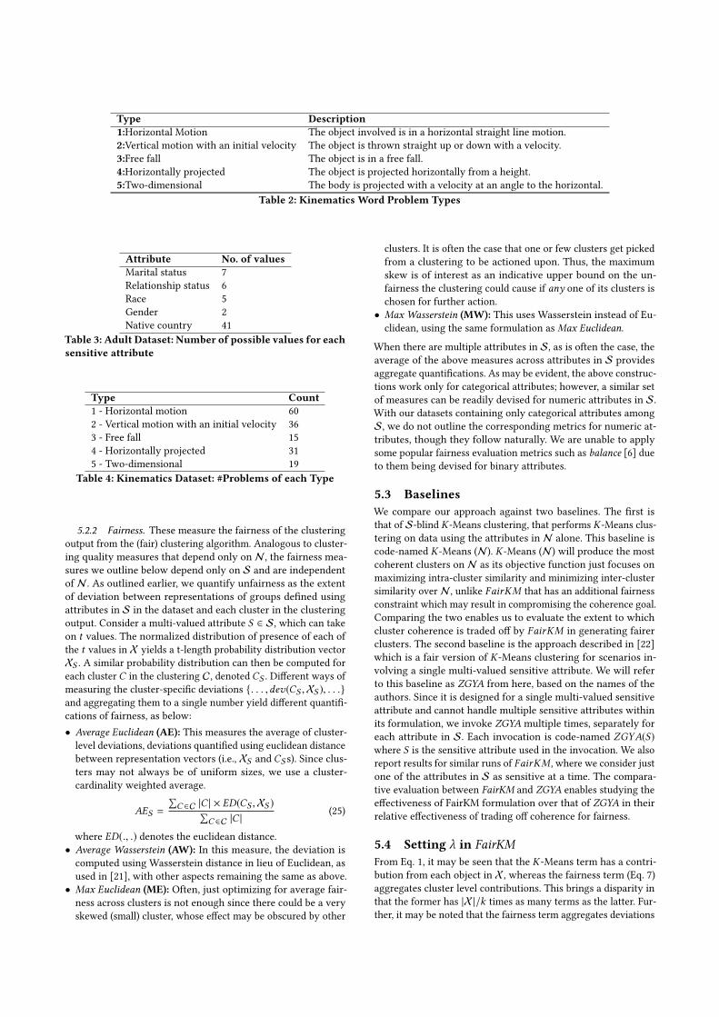
5.5.2 Clustering Quality. The clustering quality results ap-pear in Table 5 (Adult dataset) and Table 7 (Kinematics dataset),with the direction against each evaluation measure indicatingwhether lower or higher values are more desirable. For clusteringquality metrics that depend only on attributes in N , we use K-Means (N ) as a reference point since that is expected to performwell, given that it does not need to heed to S and is not heldaccountable for fairness. Thus, FairKM is not expected to beatK-Means (N ); the lesser the degradation from K-Means (N ) on

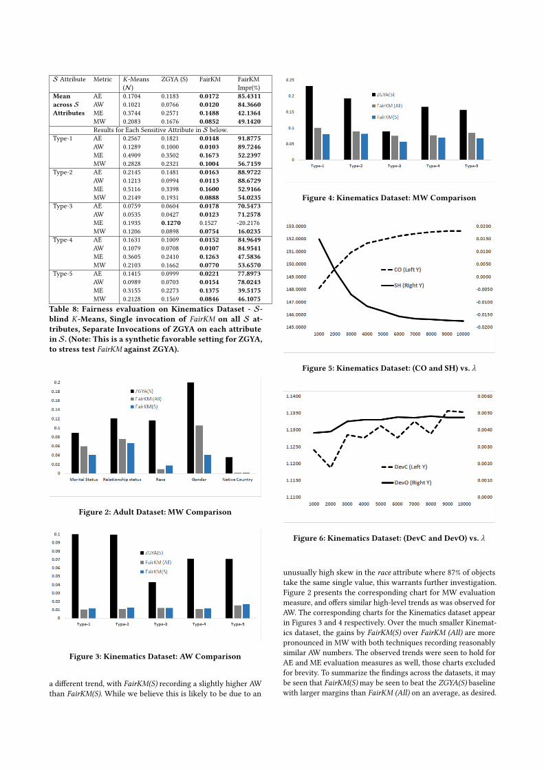
various clustering quality metrics, the better it may be regarded tobe. We compare FairKM and Avg. ZGYA across the results tables,highlighting the better performer on each evaluation measure byboldfacing the appropriate value. On the Adult dataset (Table 5),it may be seen that FairKM performs better than Avg. ZGYA onseven out of eight combinations, with it being competitive withthe latter on the eighth. FairKM is seen to score significantlybetter than Avg. ZGYA on clustering objective (CO) and silhouttescore (SH), with the gains on the deviation metrics (DevC andDevO) being more modest. It may be noted that CO and SH maybe regarded as more reliable measures, since they evaluate theclustering directly. In contrast,DevO andDevC evaluate the devi-ation against reference K-Means (N) clusterings; these deviationmeasures penalize deviations even if those be towards other goodquality clusterings that may exist in the dataset. The trends fromthe Adult dataset hold good for the Kinematics dataset as well(see Table 7), confirming that the trends generalize well acrossdatasets of widely varying character. Overall, our results indicatethat FairKM is able to generate much better quality clusteringsthan Avg. ZGYA, when gauged on attributes in N .

5.5.3 Fairness. The fairness evaluationmeasures for theAdultand Kinematics datasets appear in Tables 6 and 8 respectively; itmay be noted that lower values are desirable on all evaluationmeasures, given that they all measure deviations. In these results,which include a synthetically favorable setting forZGYA (as notedearlier), the top block indicates the average results across all at-tributes inS, with the following result blocks detailing the resultsfor the specific parameters in S. The overarching summary ofthis evaluation suggests, as indicated in the top-blocks acrossthe two tables, that FairKM surpasses the baselines with signifi-cant margins. The % impr column indicates the gain achieved byFairKM over the next best competitor. The percentage improve-ments recorded are around 35 + % on an average for the Adultdataset, whereas the corresponding figure is higher, at around60 + % for the Kinematics dataset. We wish to specifically makea few observations from the results. First, the closest competitorto FairKM is ZGYA on the Kinematics dataset, whereas K-Means(N ) curiously outperforms ZGYA quite consistently on the Adultdataset. This indicates that ZGYA is likely more suited to settingswhere the number of values taken by the sensitive attribute isless. In our case, the Kinematics dataset has all binary attributesin S, whereas Adult dataset has sensitive attributes that take asmany as 41 different values. Second, while FairKM is designedto accommodate S attributes that take many different values,the fairness deviations appear to degrade, albeit at a much lowerpace than ZGYA, as attributes take on very many values. This isindicated by the lower performance (with small margins) on thenative country (41 values) attribute at k = 5 in Table 6. However,promisingly, it is able to utilize the additional flexibility that isprovided by larger ks to ensure higher rates of fairness on them.As may be seen, FairKM recovers well to perform significantlybetter on native country at k = 15. This indicates that FairKMwill benefit from a higher flexibility in cluster assignment (withhigher k) when there are a number of (high cardinality) attributesto ensure fairness over. Third, the FairKM formulation targets tominimize overall fairness and does not specifically nudge it to-wards ensuring good performance on themaxmeasures (ME andMW) that quantify the worst deviation across clusters. Thus, it’sdesign allows to choose higher fairness in multiple clusters evenat the expense of disadvantaging fairness in one or few clusters,which is indeed undesirable. The performance on ME and MW

Evaluation k=5 k=15Measure K -Means (N) Avg. ZGYA FairKM K -Means (N) Avg. ZGYA FairKMCO ↓ 1120.9112 10791.8311 1345.1688 837.9785 4095.8366 1235.2859SH ↑ 0.7212 0.0557 0.3918 0.6076 0.0573 0.3747DevC ↓ 0.0 8.4597 8.4707 0.0 39.3615 13.1244DevO ↓ 0.0 0.0306 0.0233 0.0 0.0360 0.0256

Table 5: Clustering quality on Adult Dataset - FairKM vs. Average across {ZGYA(S)|S ∈ S}, shown with K-Means(N).

S Evaluation k=5 k=15Attribute Measure K-Means(N ) ZGYA(S) FairKM FairKM

Impr(%)K-Means(N ) ZGYA(S) FairKM FairKM

Impr(%)Mean AE 0.0459 0.1201 0.0278 39.5357 0.0537 0.1289 0.0295 45.0796across S AW 0.0161 0.0370 0.0087 45.7857 0.0194 0.0398 0.0094 51.7043Attributes ME 0.2063 0.8729 0.1457 29.4002 0.2475 0.7810 0.1542 37.6985

MW 0.0740 0.1235 0.0502 32.0985 0.0753 0.1262 0.0542 28.0040Results for Each Sensitive Attribute in S below.

Marital Status AE 0.0792 0.0886 0.0539 31.9408 0.0853 0.1318 0.0558 34.5263AW 0.0182 0.0159 0.0132 16.5650 0.0191 0.0258 0.0136 28.4239ME 0.3055 0.7356 0.2578 15.6087 0.3572 0.6365 0.2607 27.0042MW 0.0573 0.0890 0.0592 -3.3881 0.0566 0.0952 0.0604 -6.6317

Rel. Status AE 0.0711 0.1743 0.0486 31.5656 0.0808 0.1903 0.0500 38.1517AW 0.0197 0.0371 0.0146 25.8744 0.0219 0.0429 0.0150 31.3346ME 0.3331 0.7796 0.2717 18.4487 0.3823 0.7804 0.2777 27.3667MW 0.0732 0.1205 0.0760 -3.8026 0.0750 0.1439 0.0776 -3.4770

Race AE 0.0163 0.0564 0.0066 59.2251 0.0168 0.0647 0.0079 53.0164AW 0.0053 0.0154 0.0023 55.9473 0.0055 0.0162 0.0028 48.9813ME 0.0385 1.0085 0.0266 30.8822 0.0565 1.2175 0.0336 40.6276MW 0.0126 0.1159 0.0092 27.3039 0.0165 0.1142 0.0115 30.2523

Gender AE 0.0529 0.2535 0.0183 65.3039 0.0711 0.2256 0.0208 70.7472AW 0.0370 0.1153 0.0130 64.9210 0.0499 0.1122 0.0147 70.4913ME 0.3324 0.9793 0.1487 55.2713 0.4028 1.0201 0.1697 57.8731MW 0.2254 0.2568 0.1051 53.3681 0.2262 0.2671 0.1200 46.9680

Native Country AE 0.0101 0.0276 0.0113 -11.2331 0.0146 0.0323 0.0130 10.9108AW 0.0005 0.0013 0.0006 -15.2027 0.0007 0.0015 0.0006 4.7201ME 0.0221 0.8612 0.0236 -6.4585 0.0385 0.2506 0.0292 24.1555MW 0.0012 0.0354 0.0016 -25.8608 0.0020 0.0107 0.0015 25.6292

Table 6: Fairness evaluation on Adult Dataset - S-blind K-Means, Single invocation of FairKM on all S attributes, SeparateInvocations of ZGYA on each attribute in S. (Note: This is a synthetic favorable setting for ZGYA, to stress test FairKMagainst ZGYA).

Evaluation K -Means (N) Avg. ZGYA FairKMCO ↓ 145.6441 164.4703 148.1003SH ↑ 0.0390 -0.0001 0.0149DevC ↓ 0.0 1.1844 1.1241DevO ↓ 0.0 0.0032 0.0038

Table 7: Clustering quality on Kinematics Dataset - FairKMvs. Average across {ZGYA(S)|S ∈ S}, shown with K-Means(N).

suggest that such trends are not widely prevalent, with FairKMrecording reasonable gains on ME and ME. However, cases suchas marital status in Table 6 and Type-3 in Table 8 suggest that isa direction in which FairKM could improve. Finally, the overallsummary from Tables 6 and 8 suggest that FairKM delivers muchfairer clusters on S attributes, and records significant gains overthe baselines, in our empirical evaluation.

5.6 FairKM vs. ZGYAHaving compared FairKM against ZGYA for fairness in a syn-thetic setting that was favorable to the latter in the previoussection, we now do a more direct comparison here. In particu-lar, we consider comparing the FairKM and ZGYA instantiationswith each sensitive attribute separately, which offers a more level

Figure 1: Adult Dataset: AW Comparison

setting. Figure 1 illustrates the comparison on the AW evaluationmeasure over the Adult dataset for eachS attribute with ZGYA(S)and FairKM(S) values shown separated by the FairKM (All) valuein between them; all these are values obtained with k = 5. TheFairKM (All) is simply FairKM instantiated with all attributes inS, which was used in the comparison in the previous section.As may be seen, with FairKM(S) focusing on just the chosen at-tribute (as opposed to FairKM (All) that needs to spread attentionacross all attributes in S), FairKM(S) is able to achieve bettervalues for AW. Thus, FairKM(S) is seen to beat ZYGA(S) by largermargins than FairKM (All), as expected. The Race attribute shows

S Attribute Metric K-Means(N )

ZGYA (S) FairKM FairKMImpr(%)

Mean AE 0.1704 0.1183 0.0172 85.4311across S AW 0.1021 0.0766 0.0120 84.3660Attributes ME 0.3744 0.2571 0.1488 42.1364

MW 0.2083 0.1676 0.0852 49.1420Results for Each Sensitive Attribute in S below.

Type-1 AE 0.2567 0.1821 0.0148 91.8775AW 0.1289 0.1000 0.0103 89.7246ME 0.4909 0.3502 0.1673 52.2397MW 0.2828 0.2321 0.1004 56.7159

Type-2 AE 0.2145 0.1481 0.0163 88.9722AW 0.1213 0.0994 0.0113 88.6729ME 0.5116 0.3398 0.1600 52.9166MW 0.2149 0.1931 0.0888 54.0235

Type-3 AE 0.0759 0.0604 0.0178 70.5473AW 0.0535 0.0427 0.0123 71.2578ME 0.1935 0.1270 0.1527 -20.2176MW 0.1206 0.0898 0.0754 16.0235

Type-4 AE 0.1631 0.1009 0.0152 84.9649AW 0.1079 0.0708 0.0107 84.9541ME 0.3605 0.2410 0.1263 47.5836MW 0.2103 0.1662 0.0770 53.6570

Type-5 AE 0.1415 0.0999 0.0221 77.8973AW 0.0989 0.0703 0.0154 78.0243ME 0.3155 0.2273 0.1375 39.5175MW 0.2128 0.1569 0.0846 46.1075

Table 8: Fairness evaluation on Kinematics Dataset - S-blind K-Means, Single invocation of FairKM on all S at-tributes, Separate Invocations of ZGYA on each attributein S. (Note: This is a synthetic favorable setting for ZGYA,to stress test FairKM against ZGYA).

Figure 2: Adult Dataset: MW Comparison

Figure 3: Kinematics Dataset: AW Comparison

a different trend, with FairKM(S) recording a slightly higher AWthan FairKM(S). While we believe this is likely to be due to an

Figure 4: Kinematics Dataset: MW Comparison

Figure 5: Kinematics Dataset: (CO and SH) vs. λ

Figure 6: Kinematics Dataset: (DevC and DevO) vs. λ

unusually high skew in the race attribute where 87% of objectstake the same single value, this warrants further investigation.Figure 2 presents the corresponding chart for MW evaluationmeasure, and offers similar high-level trends as was observed forAW. The corresponding charts for the Kinematics dataset appearin Figures 3 and 4 respectively. Over the much smaller Kinemat-ics dataset, the gains by FairKM(S) over FairKM (All) are morepronounced in MW with both techniques recording reasonablysimilar AW numbers. The observed trends were seen to hold forAE and ME evaluation measures as well, those charts excludedfor brevity. To summarize the findings across the datasets, it maybe seen that FairKM(S)may be seen to beat the ZGYA(S) baselinewith larger margins than FairKM (All) on an average, as desired.

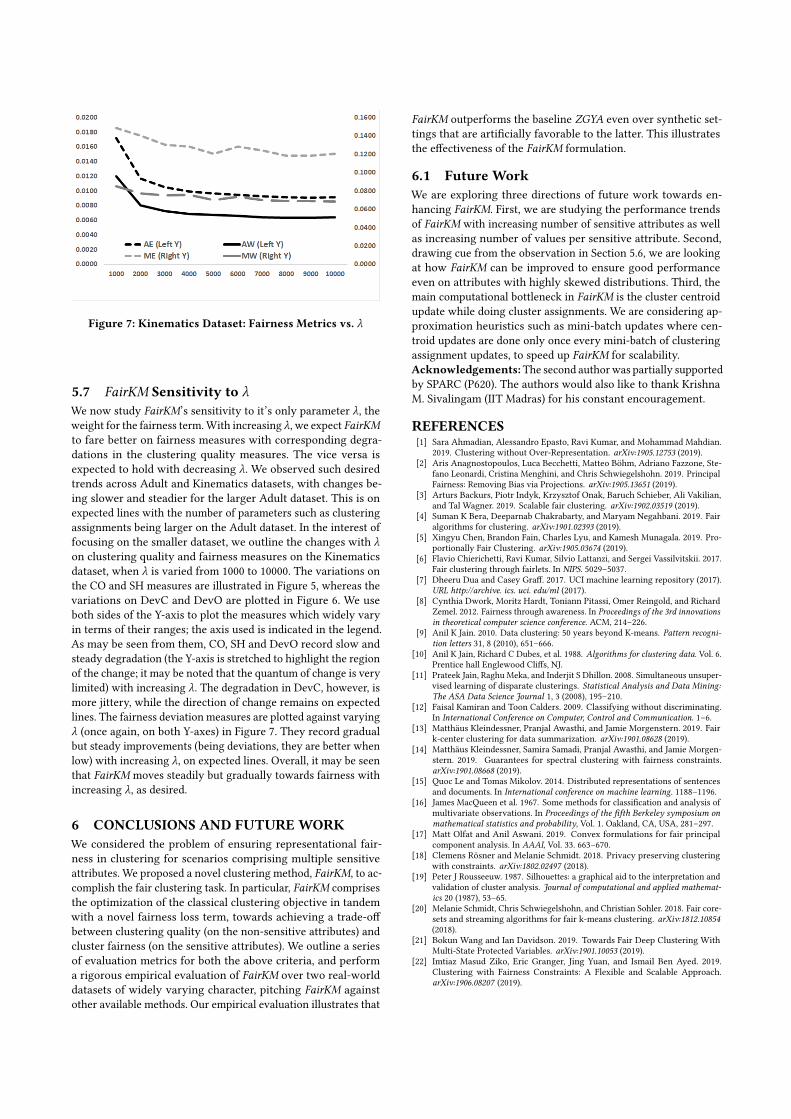
Figure 7: Kinematics Dataset: Fairness Metrics vs. λ

5.7 FairKM Sensitivity to λWe now study FairKM’s sensitivity to it’s only parameter λ, theweight for the fairness term.With increasing λ, we expect FairKMto fare better on fairness measures with corresponding degra-dations in the clustering quality measures. The vice versa isexpected to hold with decreasing λ. We observed such desiredtrends across Adult and Kinematics datasets, with changes be-ing slower and steadier for the larger Adult dataset. This is onexpected lines with the number of parameters such as clusteringassignments being larger on the Adult dataset. In the interest offocusing on the smaller dataset, we outline the changes with λon clustering quality and fairness measures on the Kinematicsdataset, when λ is varied from 1000 to 10000. The variations onthe CO and SH measures are illustrated in Figure 5, whereas thevariations on DevC and DevO are plotted in Figure 6. We useboth sides of the Y-axis to plot the measures which widely varyin terms of their ranges; the axis used is indicated in the legend.As may be seen from them, CO, SH and DevO record slow andsteady degradation (the Y-axis is stretched to highlight the regionof the change; it may be noted that the quantum of change is verylimited) with increasing λ. The degradation in DevC, however, ismore jittery, while the direction of change remains on expectedlines. The fairness deviation measures are plotted against varyingλ (once again, on both Y-axes) in Figure 7. They record gradualbut steady improvements (being deviations, they are better whenlow) with increasing λ, on expected lines. Overall, it may be seenthat FairKM moves steadily but gradually towards fairness withincreasing λ, as desired.

6 CONCLUSIONS AND FUTUREWORKWe considered the problem of ensuring representational fair-ness in clustering for scenarios comprising multiple sensitiveattributes. We proposed a novel clustering method, FairKM, to ac-complish the fair clustering task. In particular, FairKM comprisesthe optimization of the classical clustering objective in tandemwith a novel fairness loss term, towards achieving a trade-offbetween clustering quality (on the non-sensitive attributes) andcluster fairness (on the sensitive attributes). We outline a seriesof evaluation metrics for both the above criteria, and performa rigorous empirical evaluation of FairKM over two real-worlddatasets of widely varying character, pitching FairKM againstother available methods. Our empirical evaluation illustrates that

FairKM outperforms the baseline ZGYA even over synthetic set-tings that are artificially favorable to the latter. This illustratesthe effectiveness of the FairKM formulation.

6.1 Future WorkWe are exploring three directions of future work towards en-hancing FairKM. First, we are studying the performance trendsof FairKM with increasing number of sensitive attributes as wellas increasing number of values per sensitive attribute. Second,drawing cue from the observation in Section 5.6, we are lookingat how FairKM can be improved to ensure good performanceeven on attributes with highly skewed distributions. Third, themain computational bottleneck in FairKM is the cluster centroidupdate while doing cluster assignments. We are considering ap-proximation heuristics such as mini-batch updates where cen-troid updates are done only once every mini-batch of clusteringassignment updates, to speed up FairKM for scalability.Acknowledgements:The second authorwas partially supportedby SPARC (P620). The authors would also like to thank KrishnaM. Sivalingam (IIT Madras) for his constant encouragement.

REFERENCES[1] Sara Ahmadian, Alessandro Epasto, Ravi Kumar, and Mohammad Mahdian.

2019. Clustering without Over-Representation. arXiv:1905.12753 (2019).[2] Aris Anagnostopoulos, Luca Becchetti, Matteo Böhm, Adriano Fazzone, Ste-

fano Leonardi, Cristina Menghini, and Chris Schwiegelshohn. 2019. PrincipalFairness: Removing Bias via Projections. arXiv:1905.13651 (2019).

[3] Arturs Backurs, Piotr Indyk, Krzysztof Onak, Baruch Schieber, Ali Vakilian,and Tal Wagner. 2019. Scalable fair clustering. arXiv:1902.03519 (2019).

[4] Suman K Bera, Deeparnab Chakrabarty, and Maryam Negahbani. 2019. Fairalgorithms for clustering. arXiv:1901.02393 (2019).

[5] Xingyu Chen, Brandon Fain, Charles Lyu, and Kamesh Munagala. 2019. Pro-portionally Fair Clustering. arXiv:1905.03674 (2019).

[6] Flavio Chierichetti, Ravi Kumar, Silvio Lattanzi, and Sergei Vassilvitskii. 2017.Fair clustering through fairlets. In NIPS. 5029–5037.

[7] Dheeru Dua and Casey Graff. 2017. UCI machine learning repository (2017).URL http://archive. ics. uci. edu/ml (2017).

[8] Cynthia Dwork, Moritz Hardt, Toniann Pitassi, Omer Reingold, and RichardZemel. 2012. Fairness through awareness. In Proceedings of the 3rd innovationsin theoretical computer science conference. ACM, 214–226.

[9] Anil K Jain. 2010. Data clustering: 50 years beyond K-means. Pattern recogni-tion letters 31, 8 (2010), 651–666.

[10] Anil K Jain, Richard C Dubes, et al. 1988. Algorithms for clustering data. Vol. 6.Prentice hall Englewood Cliffs, NJ.

[11] Prateek Jain, Raghu Meka, and Inderjit S Dhillon. 2008. Simultaneous unsuper-vised learning of disparate clusterings. Statistical Analysis and Data Mining:The ASA Data Science Journal 1, 3 (2008), 195–210.

[12] Faisal Kamiran and Toon Calders. 2009. Classifying without discriminating.In International Conference on Computer, Control and Communication. 1–6.

[13] Matthäus Kleindessner, Pranjal Awasthi, and Jamie Morgenstern. 2019. Fairk-center clustering for data summarization. arXiv:1901.08628 (2019).

[14] Matthäus Kleindessner, Samira Samadi, Pranjal Awasthi, and Jamie Morgen-stern. 2019. Guarantees for spectral clustering with fairness constraints.arXiv:1901.08668 (2019).

[15] Quoc Le and Tomas Mikolov. 2014. Distributed representations of sentencesand documents. In International conference on machine learning. 1188–1196.

[16] James MacQueen et al. 1967. Some methods for classification and analysis ofmultivariate observations. In Proceedings of the fifth Berkeley symposium onmathematical statistics and probability, Vol. 1. Oakland, CA, USA, 281–297.

[17] Matt Olfat and Anil Aswani. 2019. Convex formulations for fair principalcomponent analysis. In AAAI, Vol. 33. 663–670.

[18] Clemens Rösner and Melanie Schmidt. 2018. Privacy preserving clusteringwith constraints. arXiv:1802.02497 (2018).

[19] Peter J Rousseeuw. 1987. Silhouettes: a graphical aid to the interpretation andvalidation of cluster analysis. Journal of computational and applied mathemat-ics 20 (1987), 53–65.

[20] Melanie Schmidt, Chris Schwiegelshohn, and Christian Sohler. 2018. Fair core-sets and streaming algorithms for fair k-means clustering. arXiv:1812.10854(2018).

[21] Bokun Wang and Ian Davidson. 2019. Towards Fair Deep Clustering WithMulti-State Protected Variables. arXiv:1901.10053 (2019).

[22] Imtiaz Masud Ziko, Eric Granger, Jing Yuan, and Ismail Ben Ayed. 2019.Clustering with Fairness Constraints: A Flexible and Scalable Approach.arXiv:1906.08207 (2019).