FairnessinCriminalJusticeRiskAssessments: TheStateoftheArt ... · FairnessinCriminalJusticeRiskAssessments: TheStateoftheArt ... The use of actuarial risk assessments in criminal

arX

iv:1

703.

0920

7v2

[st

at.M

L]

28

May

201

7 Fairness in Criminal Justice Risk Assessments:

The State of the Art

Richard Berka,b, Hoda Heidaric, Shahin Jabbaric,Michael Kearnsc, Aaron Rothc

Department of Statisticsa

Department of Criminologyb

Department of Computer and Information Sciencec

University of Pennsylvania

May 30, 2017

Abstract

Objectives: Discussions of fairness in criminal justice risk assess-ments typically lack conceptual precision. Rhetoric too often substi-tutes for careful analysis. In this paper, we seek to clarify the tradeoffsbetween different kinds of fairness and between fairness and accuracy.

Methods: We draw on the existing literatures in criminology, com-puter science and statistics to provide an integrated examination offairness and accuracy in criminal justice risk assessments. We alsoprovide an empirical illustration using data from arraignments.

Results: We show that there are at least six kinds of fairness, someof which are incompatible with one another and with accuracy.

Conclusions: Except in trivial cases, it is impossible to maximizeaccuracy and fairness at the same time, and impossible simultaneouslyto satisfy all kinds of fairness. In practice, a major complication isdifferent base rates across different legally protected groups. There isa need to consider challenging tradeoffs.

1

http://arxiv.org/abs/1703.09207v2

1 Introduction

The use of actuarial risk assessments in criminal justice settings has of latebeen subject to intense scrutiny. There have been ongoing discussions abouthow much better in practice risk assessments derived from machine learn-ing perform compared to risk assessments derived from older, conventionalmethods (Liu et al., 2011; Berk, 2012; Berk and Bleich, 2013; Brennan andOliver, 2013; Rhodes, 2013; Ridgeway, 2013a; 2013b). We have learnedthat when relationships between predictors and the response are complex,machine learning approaches can perform far better. When relationships be-tween predictors and the response are simple, machine learning approacheswill perform about the same as conventional procedures.

Far less close to resolution are concerns about fairness raised by the media(Cohen, 2012; Crawford, 2016; Angwin et al., 2016; Dietrerich et al., 2016;Doleac and Stevenson, 2016), government agencies (National Science andTechnology Council, 2016: 30-32), foundations (Pew Center of the States,2011), and academics (Demuth, 2003; Harcourt, 2007; Berk, 2009; Hyattet al., 2011; Starr, 2014b; Tonry, 2014; Berk and Hyatt, 2015; Hamilton,2016).1 Even when direct indicators of protected group membership, such asrace and gender, are not included as predictors, associations between thesemeasures and legitimate predictors can “bake in” unfairness. An offender’sprior criminal record, for example, can carry forward earlier, unjust treatmentnot just by criminal justice actors, but by an array of other social institutionsthat may foster disadvantage.

As risk assessment critic Sonja Starr writes, “While well intentioned, thisapproach [actuarial risk assessment] is misguided. The United States inar-guably has a mass-incarceration crisis, but it is poor people and minoritieswho bear its brunt. Punishment profiling will exacerbate these disparities– including racial disparities – because the risk assessments include manyrace-correlated variables. Profiling sends the toxic message that the stateconsiders certain groups of people dangerous based on their identity. It alsoconfirms the widespread impression that the criminal justice system is riggedagainst the poor” (Starr, 2014a).

On normative grounds, such concerns can be broadly legitimate, but with-out far more conceptual precision, it is difficult to reconcile competing claims

1 Many of the issues apply to actuarial methods in general about which concerns havebeen raised for some time (Berk and Messinger, 1987; Feely and Simon, 1994).

2

and develop appropriate remedies. The debates can become rhetorical exer-cises, and few minds are changed.

This paper builds on recent developments in computer science and statis-tics in which fitting procedures, often called algorithms, can assist criminaljustice decision-making by addressing both accuracy and fairness.2 Accu-racy is formally defined by out-of-sample performance using one or moreconceptions of prediction error (Hastie et al., 2009: Section 7.2). There is noambiguity. But, even when attempts are made to clarify what fairness canmean, there are several different kinds that can conflict with one another andwith accuracy (Berk, 2016b).

Examined here are different ways that fairness can be formally defined,how these different kinds of fairness can be incompatible, how risk assessmentaccuracy can be affected, and various algorithmic remedies that have beenproposed. The perspectives represented are found primarily in statistics andcomputer science because those disciplines are the source of modern riskassessment tools used to inform criminal justice decisions.

No effort is made here to translate formal definitions of fairness into philo-sophical or jurisprudential notions in part because the authors of this paperlack the expertise and in part because that multidisciplinary conversation isjust beginning (Ferguson, 2015; Barocas and Selbst, 2016; Janssen and Kuk,2016; Kroll et al., 2017). Nevertheless, an overall conclusion will be that youcan’t have it all. Rhetoric to the contrary, challenging tradeoffs are requiredbetween different kinds of fairness and between fairness and accuracy.

2 Confusion Tables, Accuracy, and Fairness

For ease of exposition and with no important loss of generality, Y is theresponse variable, henceforth assumed to be binary, and there are two pro-tected group categories: men and women. We begin by introducing by exam-ple some key ideas needed later to define fairness and accuracy. We build onthe simple structure of a 2 by 2 cross-tabulation (Berk, 2016b; Chouldechova,2016; Hardt et al., 2016). Illustrations follow shortly.

2 An algorithm is not a model. An algorithm is simply a sequential set of instructions forperforming some task. When you balance your checkbook, you are applying an algorithm.A model is an algebraic statement of how the world works. In statistics, often it representshow the data were generated.

3

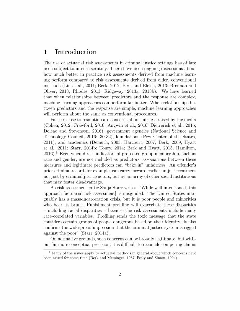
Failure Predicted Success Predicted Conditional Procedure Error

Failure – A Positive a b b/(a + b)True Positives False Negatives False Negative Rate

Success – A Negative c d c/(c + d)False Positives True Negatives False Positive Rate

Conditional Use Error c/(a + c) b/(b + d)(c+b)

(a+b+c+d)Failure Prediction Error Success Prediction Error Overall Procedure Error

Table 1: A Cross-Tabulation of The Actual Outcome by The Predicted Out-come When The Prediction Algorithm Is Applied To A Dataset

Table 1 is a cross-tabulation of the actual binary outcome Y by the pre-dicted binary outcome Y . Such tables are in machine learning often called a“confusion table” (also “confusion matrix”). Y is the fitted values that resultwhen an algorithmic procedure is applied in the data. A “failure” is called a“positive” because it motivates the risk assessment; a positive might be anarrest for a violent crime. A “success” is a “negative,” such as completinga probation sentence without any arrests. These designations are arbitrarybut allow for a less abstract discussion.3

The left margin of the table shows the actual outcome classes. The topmargin of the table shows the predicted outcome classes. Cell counts internalto the table are denoted by letters. For example, “a” is the number ofobservations in the upper-left cell. All counts in a particular cell have thesame observed outcome class and the same predicted outcome class. Forexample, “a” is the number of observations for which the observed responseclass is a failure, and the predicted response class is a failure. It is a truepositive. Starting at the upper left cell and moving clockwise around thetable are true positives, false negatives, true negatives, and false positives.

The cell counts and computed values on the margins of the table can beinterpreted as descriptive statistics for the observed values and fitted valuesin the data on hand. Also common is to interpret the computed values onthe margins of the table as estimates of the corresponding probabilities in apopulation. We turn to that later.

There is a surprising amount of information that can be extracted fromthe table. We will use the following going forward.4

3 Similar reasoning is often used in the biomedical sciences. For example, a success canbe a diagnostic test that identifies a lung tumor.

4 We proceed in this manner because there will be clear links to fairness. There aremany other measures from such a table for which this is far less true. Powers (2011)provides an excellent review.

4

1. Sample Size – The total number of observations conventionally denotedby N : a+ b+ c+ d.

2. Base Rate – The proportion of actual failures, which is (a+ b)/(a+ b+c+d), or the proportion of actual successes, which is (c+d)/(a+b+c+d)

3. Prediction Distribution – The proportion predicted to fail and the pro-portion predicted to succeed: (a+ c)/(a+ b+ c + d) and (b+ d)/(a+b+ c+ d) respectively.

4. Overall Procedure Error – The proportion of cases misclassified: (b +c)/(a+ b+ c+ d).

5. Conditional Procedure Error – The proportion of cases incorrectly clas-sified conditional on one of the two actual outcomes: b/(a + b), whichis the false negative rate, and c/(c+ d), which is the false positive rate.

6. Conditional Use Error – The proportion of cases incorrectly predictedconditional on one of the two predicted outcomes: c/(a + c), which isthe proportion of incorrect failure predictions, and b/(b + d), whichis the proportion of incorrect success predictions.5 We use the termconditional use error because when risk is actually determined, thepredicted outcome is employed; this is how risk assessments are usedin the field.

7. Cost Ratio – the ratio of false negatives to false positives b/c or theratio of false positives to false negatives c/b.

The discussion of fairness to follow uses all of these features of Table 1,although the particular features employed will vary with the kind of fairness.We will see, in addition, that the different kinds of fairness can be related toone another and to accuracy. But before getting into a more formal discus-sion, some common fairness issues will be illustrated with three hypotheticalconfusion tables.

5 There seems to be less naming consistency for these kinds errors compared to falsenegatives and false positives. Discussions in statistics about generalization error (Hastieet al., 2009: Section 7.2), can provide one set of terms whereas concerns about errors fromstatistical tests can provide another. In neither case, moreover, is the application to confu-sion tables necessarily natural. Terms like the “false discover rate” and the “false omissionrate,” or “Type II” and “Type I” errors can be instructive for interpreting statistical testsbut build in content that is not relevant for prediction errors. There is no null hypothesisbeing tested.

5

Table 2: FEMALES: FAIL(f ) OR SUCCEED(s) ON PAROLE (Success BaseRate = 500/1000 = .50, Cost ratio = 200/200 = 1:1, Predicted to Succeed500/1000 = .50)

Yf Ys Conditional Procedure Error

Yf – Positive 300 200 .40True Positives False Negatives False Negative Rate

Ys – Negative 200 300 .40False Positives True Negatives False Positive Rate

Conditional Use Error .40 .40Failure Prediction Error Success Prediction error

Table 2 is a confusion table for a hypothetical set of women released onparole. Gender is the protected individual attribute. As failure on parole isa “positive,” and a success on parole is a “negative.” For ease of exposition,the counts are meant to produce a very simple set of results.

The base rate for success is .50 because half of the women are not re-arrested. The algorithm correctly predicts that the proportion who succeedon parole is .50. This is a favorable initial indication of the algorithm’sperformance because the marginal distribution of Y and Y is the same.

The false negative rate and false positive rate of .40 is the same for suc-cesses and failures. When the outcome is known, the algorithm can correctlyidentify it 60% of the time. The cost ratio is, therefore, 1 to 1.

The prediction error of .40 is the same for predicted successes and pre-dicted failures. When the outcome is predicted, the prediction is correct 60%of the time. There is no consideration of fairness because Table 2 shows onlythe results for women.

Table 3: MALES: FAIL(f ) OR SUCCEED(s) ON PAROLE (Success BaseRate = 500/1500 = .33, Cost ratio 400/200 = 2:1, Predicted to Succeed700/1500 = .47)



Ys – Negatives 200 300 .40False Positives True Negative False Positive Rate


Table 3 is a confusion table for a hypothetical set of men released onparole. To help illustrate fairness concerns, the base rate for success on

6

parole is changed from .50 to .33. Men are substantially less likely to succeedon parole than women. The base rate was changed by multiplying the toprow of cell counts in Table 2 by 2.0. That is the only change made to thecell counts. The bottom row of cell counts are unchanged.

The false negative and false positive rates are the same and unchangedat .40. Just as for women, when the outcome is known, the algorithm cancorrectly identify it 60% of the time. We will see later that the importantcomparison is across the two tables. Having a false positive and false negativerate within a table the same, does not figure in definitions of fairness. Whatmatters is whether the false negative rate varies across tables and whetherthe false positive rate varies across tables.

Failure prediction error is reduced from .40 to .25, and success predictionerror is increased from .40 to .57. Men are more often predicted to succeedon parole when they actually don’t. Women are more often predicted to failon parole when they don’t. If predictions of success on parole make a releasemore likely, some would argue that the prediction errors unfairly favor men.Some would assert more generally that different prediction error proportionsfor men and women is by itself unfair.

Whereas in Table 2, .50 of the women are predicted to succeed, in Table 3,.47 of the men are predicted to succeed. This is a small difference in practice,but it favors women. Some would call this unfair, but it is a different kindof unfairness than disparate prediction errors by gender.

Perhaps more important, although the proportion of women predictedto succeed corresponds to the actual proportion of women who succeed, theproportion of men predicted to succeed is a substantial overestimate of theactual proportion of men who succeed. For men, the distribution Y is not thesame as the distribution of Y . Some might argue that this makes the algo-rithmic results overall less defensible for men because a kind of accuracy hasbeen sacrificed. (One would arrive at the same conclusion using predictionsof failure on parole). Fairness issues could arise if decision-makers, noting thedisparity between the actual proportion who succeed on parole and the pre-dicted proportion who succeed on parole, discount the predictions for men.Predictions of success on parole would be taken less seriously for men thanwomen.

Finally, the cost ratio in Table 2 for women makes false positives andfalse negatives equally costly (1 to 1). In Table 3, false positives are twice ascostly as false negatives. Incorrectly classifying a success on parole as failureis twice as costly for men (2 to 1). This too can be seen as unfair. Put

7

another way, individuals who succeed on parole but who would be predictedto fail, are of greater relative concern when the individual is a man.

Note, that all of these potential unfairness and accuracy problems surfacesolely by changing the base rate even when the false negative rate and falsepositive rates are unaffected. Base rates can matter a great deal, which is atheme to which we will return.

Table 4: MALES TUNED: FAIL(f ) OR SUCCEED(s) ON PAROLE (Suc-cess Base Rate = 500/1500 = .33, Cost ratio = 200/200 = 1:1, Predicted tosucceed 500/1500 = .33)



Ys – Negative 200 300 .40False Positives True Negatives False Positive Rate


We will see later that there are a number of proposals that try to correctfor various kinds of unfairness, including those illustrated in the comparisonsbetween Table 2 and Table 3. For example, it is sometimes possible to tuneclassification procedures to reduce or even eliminate some forms of unfairness.

In Table 4, the success base rate for men is still .33, but the cost ratiofor men is again 1 to 1. Now, when success on parole is predicted, it isincorrect 40 times out of 100 and corresponds to .40 success prediction errorfor women. When predicting success on parole, we have equal accuracy formen and women. One kind of unfairness has been eliminated. Moreover, thefraction of men predicted to succeed on parole now equals the actual fractionof men who succeed on parole. Some measure of credibility has been restoredto the predictions for men.

However, the false negative rate for men is now .20, not .40, as it is forwomen. In trade, therefore, when men actually fail on parole, the algorithmis more likely than for women to correctly identify it. By this measure, thealgorithm performs better for men. Tradeoffs of these kinds are endemic inclassification procedures that try to correct for unfairness. Some tradeoffsare inevitable and some are simply common. This too is a theme to whichwe will return.

8

3 The Statistical Framework

We have considered confusion tables as descriptive tools for data on hand.The calculations on the margins of the table are proportions. Yet, thoseproportions are often characterized as probabilities. Implicit are propertiesthat cannot be deduced from the data alone. Commonly, reference to a datageneration process is required (Berk, 2016: 11 – 27; Kleinberg at al., 2016).For clarity, we need to consider that data generation process.

There are practical concerns as well requiring a “generative” formulation.In many situations, one wants to draw inferences beyond the data beinganalyzed. Then, the proportions can be seen as statistical estimates. Forexample, a confusion table for release decisions at arraignments from a givenmonth, might be used to draw inferences about a full year of arraignmentsin that jurisdiction (Berk et al., 2016). Likewise, a confusion table for thehousing decisions made for prison inmates (e.g., low security housing versushigh security housing) from a given prison in a particular jurisdiction mightbe used to draw inferences about placement decisions in other prisons in thesame jurisdiction (Berk and de Leeuw, 1999).6 But perhaps most impor-tant, algorithmic results from a given dataset are commonly used to informdecisions in the future. Generalizations are needed over time.

In such circumstances, one needs a formal rationale for how the data cameto be and for the estimation target. In conventional survey sample terms,one must specify a population and one or more population parameters whosevalues are to be estimated from the data. Probability sampling then providesthe requisite justification for statistical inference.

There is a broader formulation that is usually more appropriate for algo-rithmic procedures. The formulation has each observation randomly realizedfrom a single joint probability distribution. This is a common approach incomputer science, especially for machine learning (Kearns, 1994: Section 1.2;Bishop, 2006: Section 1.5), and also can be found in econometrics (White,1980) and statistics (Freedman, 1981; Buja et al., 2017).

In this paper, we denote that joint probability distribution by P (Y, L, S).Y is the outcome of interest. An arrest while on probation is an illustration.L includes “legitimate” predictors such as prior convictions. S includes “pro-tected” predictors such as race, ethnicity and gender. In computer science,

6 The binary response might be whether an inmate is reported for serious misconductsuch as an assault on a guard or another inmate.

9

P (Y, L, S) often is called a “target population.”P (Y, L, S) has all of the usual moments. From this, the population can be

viewed as the limitless number of observations that could be realized from thejoint probability distribution (as if by random sampling), each observationan IID realized case. Under this conception of a population, all momentsand conditional moments are necessarily expectations.

There is in the population some true function of L and S, f(L, S), linkingthe predictors to the expectations of Y : E(Y |L, S). When Y is categorical,these conditional expectations are conditional probabilities. E(Y |L, S) isthe “true response surface.” The data on hand are a set of IID realizedobservations from P (Y, L, S). In some branches of computer science, such asmachine learning, each realized observation is called an “example.”

A fitting procedure, h(L, S), is applied to the data that contain a re-sponse Y . The structure of fitting procedure h(L, S) could be a linear re-gression model. The optimization algorithm could be minimizing the sumof the squared residuals by solving the normal equations. The fitted valuesafter optimization are the estimates. These concepts apply to more flexiblefitting procedures as well. For example, the structure of the machine learningprocedure gradient boosting is regression trees. The optimization algorithmis gradient descent.

We allow S to participate in the fitting procedure because it is associatedwith Y . The wisdom of proceeding in this manner is considered later whenwe address exactly what is being estimated. We denote the fitted values byY . The algorithmically produced f(L, S), which is the source of Y , is incomputer science an “hypothesis.”

For all of the usual reasons, f(L, S) will almost certainly be a biased esti-mate of the true response surface.7 For example, some important legitimatepredictions may not be available or are measured with error, and there is noguarantee whatsoever that any functional form arrived at for f(L, S) is cor-rect. Indeed, for a variety of technical reasons, the algorithms themselves willrarely provide even asymptotically unbiased estimates. For example, proce-dures that rely on ensembles of decision trees typically fit those trees with“greedy” algorithms that can make the calculations tractable at a cost offitting asymptotically biased approximations of the true response surface.8

7 Formally, a richer notational scheme should be introduced at this point, but we hopethe discussion is sufficiently clear without the clutter that would follow. See Buja and hiscolleagues (2017) for a far more rigorous treatment using proper notation.

8 Consider a single decision tree. Rather than trying all possible trees and picking the

10

This will invalidate conventional statistical tests and confidence intervals.There are ways to reformulate the inference problem that when coupled withresampling procedures can lead to proper statistical tests and confidence in-tervals, which are briefly discussed later.

Defining a population through a joint probability distribution may strikesome readers as odd. But if one is to extend empirical results beyond thedata on hand, any generalizations must be to something. Considerations ofaccuracy and fairness require such extensions because a f(L, S) developedon a given dataset will be used with new observations that it has not seenbefore.

A joint probability distribution is essentially an abstraction of a high-dimensional histogram from a finite population. It is just that the number ofobservations is now limitless, and there is no binning.9 We imagine that thedata are realized by the equivalent of random sampling. We say that the dataare realized independently from the same distribution, sometimes denotedby IID for independently and identically distributed. Proper estimation canfollow, but now with inferences drawn to an infinite population, or with thesame reasoning, to the joint probability distribution that characterizes it.

Whether this perspective on estimation makes sense for real data dependson substantive knowledge and knowledge about how the data were actuallyproduced. For example, one might be able to make the case that for aparticular jurisdiction, all felons convicted in a given year can usefully be seenas IID realizations from all convicted felons that could have been producedthat year and perhaps for a few years before and a few years after. Onewould need to argue that for the given year, or proximate years, there wereno meaningful changes in any governing statutes, the composition of thesitting judges, the mix of felons, and the practices of police, prosecutors, anddefense attorneys. A more detailed consideration would for this paper bea distraction, and is discussed elsewhere in an accessible, linear regression

tree with the best performance, the fitting proceeds in a sequential stagewise fashion. Asthe tree is grown, earlier branches are not reconsidered as later branches are determined(Hastie et al., 2009: Section 9.2).

9 As a formal matter, when all of the variables are continuous, the proper term is a jointdensity because densities rather than probabilities are represented. When the variablesare all discrete, the proper term is a joint probability distribution because probabilities arerepresented. When one does not want to commit to either or when some variables are con-tinuous and some are discrete, one commonly uses the term joint probability distribution.That is how we proceed here.

11

setting (Berk et al., 2017).

4 Defining Fairness

4.1 Definitions of Algorithmic Fairness

We are now ready to consider definitions of algorithmic fairness. Instructivedefinitions can be found in computer science (Pedreschi, 2008; Kamishimaet al., 2011; Dwork et al., 2012; Kamiran et al., 2012; Chouldechova, 2016;Friedler et al., 2016; Hardt et al., 2016; Joseph et al., 2016; Kleinberg et al.,2016; Calmon et al., 2017; Corbitt-Davies et al., 2017), criminology (Berk,2016b; Angwin et al., 2016; Dieterich et al., 2016) and statistics (Johnsonet al., 2016; Johndrow and Lum, K. 2017). All are recent and focused onalgorithms used to inform real-world decisions in both public and privateorganizations.

All of the definitions are broadly similar in intent. What matters is thetreatment of protected groups. But the definitions can differ in substantiveand technical details. There can be frustrating variation in notation com-bined with subtle differences in how key concepts are operationalized. Therealso can be a conflation of information provided by an algorithm and deci-sions that can follow.10 We focus here on algorithms. How those can affectdecisions is a very important, but different matter (Berk, 2017; Kleinberg etal., 2017).

Our exposition is agnostic with respect to how outcome classes are as-signed by an algorithm and about the fitting procedure used. This is inthe spirit of work by Kleinberg and his colleagues (2016). The notation isarithmetically based to facilitate accessibility.

In order to provide clear definitions of algorithmic fairness, we will pro-ceed for now as if f(L, S) provides estimates that are the same as the corre-sponding population features. In this way, we do not conflate a discussion offairness with a discussion of estimation accuracy. The estimation accuracyis addressed later. We draw heavily on our earlier discussion of confusion ta-bles, but to be consistent with the fairness literature, we emphasize accuracyrather than error. Nevertheless, the notation is drawn from Table 1. Finally,

10 The meaning of “decision” can vary. For some it is assigning an outcome class to anumeric risk score. For others, it is an concrete action taken with the information providedby a risk assessment.

12

in applications, there will be a separate confusion table for each class in theprotected group. Comparisons are made between these tables.

1. Overall accuracy equality is achieved by f(L, S) when overall procedureaccuracy is the same for each protected group category (e.g., men andwomen). That is, (a+d)/(a+b+c+d) should be the same (Berk, 2016b).This definition assumes that true negatives are as desirable as truepositives. In many settings they are not, and a cost-weighted approachis required. For example, true positives may be twice as desirable astrue negatives. Or put another way, false negatives may be two timesmore undesirable than false positives. Overall accuracy equality is notcommonly used because it does not distinguish between accuracy forsuccesses and accuracy for failures. Nevertheless, it has been mentionedin some media accounts (Angwin et al., 2016), and is related in spiritto “accuracy equity” as used by Dieterich and colleagues (2016).11

2. Statistical parity is achieved by f(L, S) when the marginal distribu-tions of the predicted classes are the same for both protected groupcategories. That is, (a+ c)/(a+ b+ c+ d) and (b+ d)/(a+ b+ c+ d),although typically different from one another, are the same for bothgroups (Berk, 2016b). For example, the proportion of inmates pre-dicted to succeed on parole should be the same for men and womenparolees. When this holds, it also holds for predictions of failure onparole because the outcome is binary. This definition of statistical par-ity, sometimes called “demographic parity,” has been properly criticizedbecause it can lead to highly undesirable decisions (Dwork et al., 2012).One might incarcerate women who pose no public safety risk so thatthe same proportions of men and women are released on probation.

3. Conditional procedure accuracy equality is achieved by f(L, S) whenconditional procedure accuracy is the same for both protected groupcategories (Berk, 2016b). In our notation, a/(a + b) is the same for

11 Dieterich and his colleagues (2016: 7) argue that overall there is accuracy equitybecause “the AUCs obtained for the risk scales were the same, and thus equitable, forblacks and whites.” The AUC depends on the true positive rate and false positive rate,which condition on the known outcomes. Consequently, it differs formally from overallaccuracy equality. Moreover, there are alterations of the AUC that can lead to moredesirable performance measures (Powers, 2011).

13

men and women, and d/(c+ d) is the same for men and women. Con-ditioning on the known outcome, is f(L, S) equally accurate acrossprotected group categories? This is the same as considering whetherthe false negative rate and the false positive rate, respectively, is thesame for men and women. Conditional procedure accuracy equalityis a common concern in criminal justice applications (Dieterich et al.,2016). Hardt and his colleagues (2016: 2-3) use the term “equalizedodds” for a closely related definition, and there is a special case theycall “equality of opportunity” that effectively is the same as our condi-tional procedure accuracy equality, but only for the outcome class thatis more desirable.12

4. Conditional use accuracy equality is achieved by f(L, S) when condi-tional use accuracy is the same for both protected group categories(Berk., 2016b). One is conditioning on the algorithm’s predicted out-come not the actual outcome. That is, a/(a+c) is the same for men andwomen, and d/(b+d) is the same for men and women. Conditional useaccuracy equality has also been a common concern in criminal justicerisk assessments (Dieterich et al., 2016). Conditional on the predictionof success (or failure), is the probability of success (or failure) the sameacross groups? Kleinberg and colleagues (2016: 2-4) have a closely re-lated definition that builds on “calibration.” More will be said aboutcalibration later. Chouldechova (2016: section 2.1) arrives at a defi-nition that is the same as conditional use accuracy equality but alsoonly for the outcome class labeled “positive.” Her “positive predictivevalue” corresponds to our a/(a+ c).13

5. Treatment equality is achieved by f(L, S) when the ratio of false nega-tives and false positives (i.e., c/b or b/c) is the same for both protectedgroup categories. The term “treatment” is used to convey that such

12 One of the two outcome classes is deemed more desirable, and that is the outcome classfor which there is conditional procedure accuracy equality. In criminal justice settings, itcan be unclear which outcome class is more desirable. Is an arrest for burglary more orless desirable than an arrest for a straw purchase of a firearm? But if one outcome classis recidivism and the other outcome class is no recidivism, equality of opportunity refersto conditional procedure accuracy equality for those who did not recidivate.

13 As noted earlier, “positive” refers to the outcome class that motivates the classificationexercise. That outcome class does not have to desirable. We have been calling the outcomeclass recidivism “positive.”

14

ratios can be a policy lever with which to achieve other kinds of fair-ness. For example, if false negatives are taken to be more costly formen than women so that conditional procedure accuracy equality canbe achieved, men and women are being treated differently by the al-gorithm. Incorrectly classifying a failure on parole as a success, say, isa bigger mistake for men. The relative numbers of false negatives andfalse positives across protected group categories also can by itself beviewed as a problem in criminal justice risk assessments (Angwin et al.,2016). Chouldechova (2016: section 2.1) addresses similar issues, butthrough the false negative rate and the false positive rate: our b/(a+b)and c/(c+ d), respectively.

6. Total fairness is achieved by f(L, S) when (1) overall accuracy equality,(2) statistical parity, (3) conditional procedure accuracy equality, (4)conditional use accuracy equality, and (5) treatment equality are allachieved. Although a difficult pill for some to swallow, we will see thatin practice, total fairness cannot be achieved.

Each of the definitions of fairness apply when there are more than twooutcome categories. However, there are more statistical summaries that needto be reviewed. For example, when there are three response classes, there arethree ratios of false negatives to false positives to be examined. There arealso other definitions of fairness not discussed because they currently cannotbe operationalized in a useful manner. For example, nearest neighbor parityis achieved if similarly situated individuals are treated similarly (Dwork etal., 2012). Similarly situated is measured by the Euclidian distance betweenthe individuals in predictor space. Unfortunately, the units in which thepredictors are measured can make an important difference, and standardizingthem just papers over the problem. This is a well-known difficulty with allnearest neighbor methods (Hastie et al., 2009: Chapter 13).

5 Estimation Accuracy

We build now on work by Buja and his colleagues (2017). When the proce-dure h(L, S) is applied to the IID data, the resulting f(L, S) can be seen asestimating the true response surface. But even asymptotically, there is nocredible claim that the true response surface is being estimated in an unbi-ased manner. The same applies to the probabilities from a cross-tabulation

15

of Y by Y . With larger samples, the random estimation error is smaller. Onthe average, the estimates are closer to the truth. However, the gap betweenthe estimates and the truth combines bias and variance. That gap is not aconventional confidence interval, nor can it be transformed into one. Onewould have to remove the bias, and to remove the bias, one would need tocompare the estimates to the truth. But, the truth is unknown.14

Alternatively, f(L, S) can also be seen estimating a response surface inthe population that is an acknowledged approximation of the true responsesurface. In the population, the approximation has the same form as f(L, S).Therefore, the estimates of probabilities from Table 1 can be estimates of thecorresponding probabilities from a Y by Y cross-tabulation if h(L, S) wereapplied in the population. Thanks to the IID nature of the data, these esti-mates can also be asymptotically unbiased so that in large samples, the biaswill likely be relatively small. This allows one to use sample results to addressfairness as long as one appreciates that it is fairness measured by the approx-imation, not the true E(Y |L, S). Because it is the performance of f(L, S)that matters, a focus on f(L, S) is consistent with policy applications.15

For either estimation target, estimation accuracy is addressed by out-sample-performance. Fitted values in-sample will be subject to overfitting.In practice, this means using test data, or some good approximation thereof,with measures of fit such as generalization error or expected prediction error(Hastie et al., 2006: Section 7.2). Often, good estimates of accuracy may beobtained, but the issues can be tricky. Depending on the procedure h(L, S)and the availability of an instructive form of test data, there are differenttools that vary in their assumptions and feasibility (Berk, 2016a). With ourfocus on fairness, such details are a diversion.

In summary, h(L, S) can best be seen as a procedure to approximate thetrue response surface. If the estimation target is the true response surface,the estimates will be biased although random estimation error will be smallerin larger samples. It follows that the probabilities estimated from a cross-

14 If the truth were known, there would be need for the estimates.15 There are technical details that are beyond the scope of this paper. Among the key

issues is how the algorithm is tuned and the availability of test data as well as training data(Berk, 2016a). There are also disciplinary differences in how important it is to explicitlyestimate features of the approximation. For many statisticians, having an approximationas an estimation target is desirable because one can obtain asymptotically the usual arrayof inferential statistics. For many computer scientists, such statistics are of little interestbecause what really matters is estimates of the true response surface.

16

tabulation of Y by Y will have the same strengths and weaknesses. If theestimation target is the acknowledged approximation, the approximate re-sponse surface can be estimated in an asymptotically unbiased manner withless random estimation error the larger the sample size. This holds for theprobabilities computed from a cross-tabulation of Y by Y . Under eitherestimation target, proper measures of accuracy often can be obtained withtest data or methods that approximate test data such as the nonparametricbootstrap (Hastie et al., 2009: Section 8.2).

6 Tradeoffs

We turn to tradeoffs and begin by emphasizing an obvious point that canget lost in discussions of fairness. If the goal of applying h(L, S) is to cap-italize on non-redundant associations that L and S have with the outcome,excluding S will reduce accuracy. Any procedure that even just discountsthe role of S will lead to less accuracy. The result is a larger number of falsenegatives and false positives. For example, if h(L) is meant to help informparole release decisions, there will likely be an increase in both the number ofinmates who are unnecessarily detained and the number of inmates who areinappropriately released. The former victimizes inmates and their families.The latter increases the number of crime victims. But fairness counts too,so we need to examine tradeoffs.

Because the different kinds of fairness defined earlier share cell countsfrom the cross-tabulation of Y against Y , and because there are relation-ships between the cell counts themselves (e.g., they sum to the total numberof observations), the different kinds of fairness are related as well. It shouldnot be surprising, therefore, that there can be tradeoffs between the differentkinds of fairness. Arguably, the tradeoff that has gotten the most atten-tion is between conditional use accuracy equality and the false positive andfalse negative rates (Angwin et al., 2016; Dieterich, 2016; Kleinberg et al.,2016; Chouldechova, 2016). It is also the tradeoff that to date has the mostcomplete mathematical results.

6.1 Some Proven “Impossibility Theorems”

We have conveyed informally that there are incompatibilities between dif-ferent kinds of fairness. It is now time to be specific. We begin with three

17

definitions. They will be phrased in probability terms, but are effectively thesame if phrased in terms of proportions.

• Calibration – Suppose an algorithm produces a score that can then beused to assign an outcome class, much in the spirit of the COMPASinstrument. “Calibration within groups” requires that for each scorevalue, or for proximate score values, the proportion of people who actu-ally experience a given outcome (e.g., re-arrested in parole) is the sameas the proportion of people predicted to experience that outcome. Asnoted earlier, this can be taken as an indicator of how well an algo-rithm performs. But calibration can become a fairness matter if thereis calibration within one group but not within the other. There is alack of “balance.” A decision-maker may be inclined to take the pre-dictions less seriously for the group that lacks calibration (Kleinberget al., 2016). Even if there is no calibration for either group, differentconditional use accuracy has been a salient concern in criminal justiceapplications and will be emphasized here (Chouldechova, 2016).16

• Base Rate – This too was introduced earlier. In the population, baserates are determined by the marginal distribution of the response. Theyare the probability of each outcome class. For example, the base ratefor succeeding on parole might be .65 and for not succeeding on paroleis then .35. If there are C outcome classes, there will be C base rates.

We are concerned here with base rates for different protected groupcategories, such as men compared to women. Base rates for each pro-tected group category are said to be equal if they are identical. Is theprobability of succeeding on parole .65 for both men and women?

• Separation – In a population, the observations are separable if for eachpossible configuration of predictor values, there is some h(L, S) forwhich the probability of membership in a given outcome class is alwayseither 1.0 or 0.0. In other words, perfectly accurate classification is pos-sible. In practice, what matters is whether there is perfect classificationwhen h(L, S) is applied to data.

And now the impossibility result: When the base rates differ by protected

group and when there is not separation, one cannot have both conditional

16 There is a bit of definitional ambiguity because Chouldechova (2016: 2) characterizesequal conditional use accuracy as “well-calibrated.”

18

use accuracy equality and equality in the false negative and false positive

rates (Kleinberg et al., 2016; Chouldechova, 2016).17 Put more positively,one needs either equal base rates or separation to achieve at the same timeconditional use accuracy equality and equal false positive and false negativerates for each protected group category.

The implications of this impossibility result are huge. First, if thereis variation in base rates and no separation, you can’t have it all. Thegoal of complete race or gender neutrality is unachievable. In practice, bothrequirements are virtually never met, except in highly stylized examples.

Second, altering a risk algorithm to improve matters can lead to difficultstakeholder choices. If it is essential to have conditional use accuracy equality,the algorithm will produce different false positive and false negative ratesacross the protected group categories. Conversely, if it is essential to havethe same rates of false positives and false negatives across protected groupcategories, the algorithm cannot produce conditional use accuracy equality.Stakeholders will have to settle for an increase in one for a decrease in theother. To see how all of this can play out, consider the following didacticillustrations.

6.1.1 Trivial Case #1: Assigning the Same Outcome Class to All

Suppose h(L, S) assigns the same outcome class to everyone (e.g., a failure).Such an assignment procedure would never be used in practice, but it raisessome important issues in a simple setting.

Tables 5 and 6 provide an example when the base rates are the samefor men and women. There are 500 men and 50 women, but the relativerepresentation of men and women does not matter materially in what follows.Failures are coded 1 and successes are coded 0, much as they might be inpractice. Each case is assigned failure (i.e., Y = 1), but the same lessonswould be learned if each case is assigned a success (i.e., Y = 0). A base rateof .80 for failures is imposed on both tables.

In practice, this approach makes no sense. Predictors are not being ex-

17 This impossibility theorem is formulated a little differently by Kleinberg and hiscolleagues and by Chouldechova. Kleinberg et al. (2016) impose calibration and makeexplicit use of a risk scores from the algorithm. There is no formal transition to outcomeclasses. Chouldechova (2016), does not impose calibration in the same sense, and movesquickly from risk scores to outcome classes. But both sets of results are for our purposeseffectively the same and consistent with our statement.

19

Table 5: Males: A Cross-Tabulation When All Cases Are Assigned TheOutcome Of Failure (Base Rate = .80, N = 500)

Truth Y = 1 Y = 0 Conditional Procedure AccuracyY = 1 (a positive – Fail) 400 0 1.0Y = 0 (a negative – Not Fail) 100 0 0.0Conditional Use Accuracy .80 –

Table 6: Females: A Cross-Tabulation When All Cases Are Assigned TheOutcome of Failure (Base Rate = .80, N = 50)

Truth Y = 1 Y = 0 Conditional Procedure AccuracyY = 1 (a positive – Fail) 40 0 1.0Y = 0 (a negative – Not Fail) 10 0 0.0Conditional Use Accuracy .80 –

ploited. But, one can see that there is conditional procedure accuracy equal-ity, conditional use accuracy equality and overall accuracy equality. The falsenegative and false positive rates are the same for men and women as well at0.0 and 1.0. There is also statistical parity. One does very well on fairnessfor a risk tool that cannot help decision-makers address risk in a useful man-ner. Accuracy has been given a very distant backseat. There is a dramatictradeoff between accuracy and fairness.

If one allows the base rates for men and women differ, there is immediatelya fairness price. Suppose in Table 5, 500 men fail instead of 400. The falsepositive and false negative rates are unchanged. But because the base rate formen is now larger than the base rate for women (i.e., .83 v. .80), conditionaluse accuracy is now higher for men, and a lower proportion of men will beincorrectly predicted to fail. This is the sort of result that would likely triggercharges of gender bias. Even in this “trivial” case, base rates matter.18

18 When base rates are the same in this example, one perhaps could not achieve perfectfairness while also getting perfect accuracy. The example doesn’t have enough informationto conclude that the populations aren’t separable. But that is not the point we are tryingto make.

20

6.1.2 Trivial Case #2: Assigning the Classes Using the Same

Probability for All

Suppose each case is assigned to an outcome class with the same probability.As in Trivial Case #1, no use made of predictors, so that accuracy does notfigure into the fitting process.

For Tables 7 and 8, the assignment probability for failure is .30 for all,and therefore, the assignment probability for success is .70 for all. Nothingimportant changes should some other probability be used.19 The base ratesfor men and women are the same. For both, the proportions that fail are .80.

Table 7: Males: A Cross-Tabulation With Failure Assigned To All With AProbability of .30 (Base Rate = .80, N = 500)

Truth Y = 1 Y = 0 Conditional Procedure AccuracyY = 1 (a positive – Fail) 120 280 .30Y = 0 (a negative – Not Fail) 30 70 .70Conditional Use Accuracy .80 .20

Table 8: Females: A Cross-Tabulation With Failure Assigned To All WithA Probability of .30 (Base Rate = .80, N = 50)


In Tables 7 and 8, we have the same fairness results we had in Tables 5and 6, again with accuracy sacrificed. But suppose the second row of entriesin Table 8 were 30 and 70 rather than 3 and 7. Now the failure base ratefor women is .29, not .80. Conditional procedure accuracy equality remainsfrom which it follows that the false negative and false positive rates are the

19 The numbers in each cell assume for arithmetic simplicity that the counts come outexactly as they would in a limitless number of realizations. In practice, an assignmentprobability of .30 does not require exact cell counts of 30%.

21

same as well. But conditional use accuracy equality is lost. The probabilitiesof correct predictions for men are again .80 for failures, and .20 for successes.But for women, the corresponding probabilities are .29 and .71. Base ratesreally matter.

6.1.3 Perfect Separation

We now turn to an h(L, S) that is not trivial, but also very unlikely inpractice. In a population, the observations are separable. In Tables 9 and10, there is perfect separation, and h(L, S) finds it. Base rates are the samefor men and women: .80 fail.

Table 9: Males: A Cross-Tabulation With Separation and Perfect Prediction(Base Rate = .80, N = 500)

Truth Y = 1 Y = 0 Conditional Procedure AccuracyY = 1 (a positive – Fail) 400 0 1.0Y = 0 (a negative – Not Fail) 0 100 1.0Conditional Use Accuracy 1.0 1.0

Table 10: Females: A Cross-Tabulation With Separation and Perfect Predic-tion (Base Rate = .80, N = 50)

Truth Y = 1 Y = 0 Conditional Procedure AccuracyY = 1 (a positive – Fail) 40 0 1.0Y = 0 (a negative – Not Fail) 0 10 1.0Conditional Use Accuracy 1.0 1.0

There are no false positives or false negatives, so the false positive rateand the false negative rate for both men and women are 0.0. There is con-ditional procedure accuracy equality and conditional use accuracy equalitybecause conditional procedure accuracy and conditional use accuracy areboth perfect. This is the ideal, but fanciful, setting in which we can have itall.

Suppose for women in Table 10, there are 20 women who do not failrather than 10. Their failure base rate for females is now .67 rather than

22

.80. But because of separation, conditional procedure accuracy equality andconditional use accuracy equality remain, and the false positive and falsenegative rates for men and women are still 0.0. Separation saves the day.20

6.1.4 Closer To Real Life

There will virtually never be separation in the real data even if there therehappens to be separation in the joint probability distribution responsiblefor the data. The fitting procedure h(L, S) may be overmatched becauseimportant predictors are not available or because the algorithm arrives ata suboptimal result. Nevertheless, some types of fairness can sometimes beachieved if base rates are cooperative.

If the base rates are the same and h(L, S, ) finds that, there can be lotsof good news. Tables 11 and 12 illustrate. Conditional procedure accuracyequality, conditional use accuracy equality, overall procedure accuracy hold,and the false negative rate and the false positive rate are the same for menand women. Results like those shown in Tables 11 and 12 can occur inreal data, but would be rare in criminal justice applications for the commonprotected groups. Base rates will not be the same.

Table 11: Females: A Cross-Tabulation Without Separation (Base Rate =.56, N = 900)


Suppose there is separation but the base rates are not the same. We areback to Tables 9 and 10, but with a lower base rate. Suppose there is noseparation, but the base rates are the same. We are back to Tables 11 and12.

From Tables 13 and 14, one can see that when there is no separationand different base rates, there can still be conditional procedure accuracyequality. From conditional procedure accuracy equality, the false negative

20 Although statistical parity has not figured in these illustrations, changing the baserate negates it.

23

Table 12: Males: Confusion Table Without Separation (Base Rate is = .56,N = 1400)


Table 13: Confusion Table For Females With No Separation And A DifferentBase Rate Compared to Males (Female Base Rate Is 500/900 = .56)


rate and false positive rate, though different from one another, are the sameacross men and women. This is a start. But treatment equality is gone fromwhich it follows that conditional use accuracy equality has been sacrificed.There is greater conditional use accuracy for women.

Table 14: Confusion Table for Males With No Separation And A differentBase Rate Compared to Females (Male Base Rate Is 1000/2200 = .45)


Of the lessons that can be taken from the sets of tables just analyzed,perhaps the most important for policy is that when there is a lack of separa-tion and different base rates across protected group categories, a key tradeoffwill be between the false positive and false negative rates on one hand andconditional use accuracy equality on the other. Different base rates across

24

protected group categories would seem to require a thumb on the scale ifconditional use accuracy equality is to be achieved. To see if this is true,we now consider corrections that have been proposed to improve algorithmicfairness.

7 Potential Solutions

There are several recent papers that have proposed ways to reduce and eveneliminate certain kinds of bias. As a first approximation, there are threedifferent strategies (Hajian and Domingo-Ferrer, 2013), although they canalso be combined when accuracy as well as fairness are considered.

7.1 Pre-Processing

Pre-processing means eliminating any sources of unfairness in the data beforeh(L, S) is formulated. In particular, there can be legitimate predictors thatare related to the classes of a protected group. Those problematic associa-tions can be carried forward by the algorithm.

One approach is to remove all linear dependence between L and S (Berk,2009). One can regress in turn each predictor in L on the predictors in S, andthen work with the their residuals. For example, one can regress predictorssuch as prior record and current charges on race and gender. From the fittedvalues, one can construct “residualized” transformations of the predictors tobe used.

A major problem with this approach is that interactions effects (e.g.,with race and gender) containing information leading to unfairness are notremoved unless they are explicitly included in the residualizing regressioneven if all of the additive contaminants are removed. In short, all interactionseffects, even higher order ones, would need to anticipated. The approachbecomes very challenging if interaction effects are anticipated between L andS.

Johndrow and Lum (2017) suggest a far more sophisticated residualizingprocess that in principle can handle such complications. Fair prediction isdefined as constructing fitted values for some outcome using no informationfrom membership in any protected classes. The goal is to transform all pre-dictors so that fair prediction can be obtained “while still preserving as much‘information’ in X as possible (Johndrow and Lum, 2017: 6). They formu-

25

late this using the Euclidian distance between the original predictors and thetransformed predictors. The predictors are placed in order of the complexityof their marginal distribution, and each is residualized in turn using as pre-dictors results from previous residualizations and indicators for the protectedclass. The regressions responsible for the residualizations are designed to beflexible so that nonlinear relationships can be exploited. But, as Johnson andLum note, they are only able to consider one form of unfairness. In addition,they risk exacerbating one form of unfairness while mitigating another.

Base rates that vary over protected group categories can be another sourceof unfairness. A simple fix is to rebalance the marginal distributions of theresponse variable so that the base rates for each category are the same. Onemethod is to apply weights for each group separately so that the base ratesacross categories are the same. For example, women who failed on parolemight given more weight, and males who failed on parole might be given lessweight. After the weighting, men and women could have a base rate thatwas the same as the overall base rate.

A second rebalancing method is to randomly relabel some response valuesto make the base rates comparable. For example, one could for a randomsample of men who failed on parole, recode the response to a successes andfor a random sample of women who succeeded on parole, recode the responseto a failure.

Rebalancing has at least two problems. First, there is likely to be a lossin accuracy. Perhaps such a tradeoff between fairness and accuracy will beacceptable to stakeholders, but before such a decision is made, the trade-off must be made numerically specific. How many more armed robberies,for instance, will go unanticipated in trade for a specified reduction in thedisparity between incarceration rates for men and women? Second, rebalanc-ing implies using different false positive to false negative rates for differentprotected group categories. For example, false positives (e.g., incorrectlypredicting that individuals will fail on parole) are treated as relatively moreserious errors for men than for women. In addition to the loss in accuracy,stakeholders are trading one kind of unfairness for another.

A third approach capitalizes on association rules, popular in marketingstudies (Hastie et al., 2009: section 14.2). Direct discrimination is addressedwhen features of some protected class are used as predictors (e.g., male).Indirect discrimination is addressed when predictors are used that are relatedto those protected classes (e.g., arrests for aggravated assault). There can beevidence of either if the conditional probability of the outcome changes when

26

either direct or indirect measures of protected class membership are used aspredictors compared to when they are not used. One potential correctioncan be obtained by perturbing the suspect class membership (Pedreschi etal., 2008). For a random set of cases, one might change the label for manto the label for a woman. Another potential correction can be obtainedby perturbing the the outcome label. For a random set of men, one mightchange failure on parole to success on parole (Hajian and Domingo-Ferrer,2013). Note that the second approach changes the base rate. We examinedearlier the consequences of changing base rates. Several different kinds offairness can be affected. It can be risky to focus on a single definition offairness.

A fourth approach is perhaps the most ambitious. The goal is to randomlytransform all predictors except for indicators of protected class membershipso that the joint distribution of the predictors is less dependent on protectedclass membership. An appropriate reduction in dependence is a policy deci-sion. The reduction of dependence is subject to two constraints: (1) the jointdistribution of the transformed variables is very close to the joint distribu-tion of the original predictors and (2) no individual cases are substantiallydistorted because large changes are made in predictor values (Calmon et al.,2017). An example of a distorted case would be a felon with no prior arrestsassigned a predictor value of 20 prior arrests. It is unclear, however, howthis procedure maps to different kinds of fairness. For example, the trans-formation itself may inadvertently treat prior crimes committed by men asless serious than similar prior crimes committed by women – the transforma-tion may be introducing the prospect of unequal treatment. There are alsoconcerns about the accuracy price, which is not explicitly taken into account.

7.2 In-Processing

In-processing means making fairness adjustments as part of the process bywhich h(L, S) is constructed. To take a simple example, risk forecasts forparticular individuals that have substantial uncertainty can be altered toimprove fairness. If whether or not an individual is projected as high riskdepends on little more than a coin flip, the forecast of high risk can bechanged to low risk to serve some fairness goal. One might even order casesfrom low certainty to high certainty for the class assigned so that low certaintyobservations are candidates for alterations first. The reduction in out-of-sample accuracy may well be very small. One can embed this idea in a

27

classification procedure so that explicit tradeoffs are made (Kamiran andCalder, 2009; Kamiran et al., 2016; Corbett-Davies et al. 2017). But this toocan have unacceptable consequences for the false positives and false negativerates. A thumb is being put on the scale once again, so there can be inequalityof treatment.

A more technically demanding approach is to add a new penalty term toa penalized fitting procedure (Kamishima et al., 2011). Beyond a penaltyfor an unnecessarily complex fit, there is a penalty for violations of condi-tional procedure accuracy equality. One important complication is that theloss function typically will not be convex so that local solutions can result.Another important complication is that there will often be undesirable im-plications for types of unfairness not formally taken into account.

7.3 Post-Processing

Post-processing means that after h(L, S) is applied, its performance is ad-justed to make it more fair. To date, perhaps the best example of this ap-proach draws on the idea of random reassignment of the class label previouslyassigned by h(L, S) (Hardt et al., 2016). Fairness, called “equalized odds,”requires that the fitted outcome classes (e.g., high risk or low risk) are inde-pendent of protected class membership, conditioning on the actual outcomeclasses. The requisite information is obtained from the rows of confusion ta-ble and, therefore, represent classification accuracy, not prediction accuracy.There is a more restrictive definition called “equal opportunity” requiringsuch fairness only for the more desirable of the two outcome classes.21

For a binary response, some cases are assigned a value of 0 and someassigned a value of 1. To each is attached a probability of switching from a0 to a 1 or from a 1 to a 0 depending in whether a 0 and a 1 is the outcomeassigned by f(L, S). These probabilities can differ from one another andboth can differ across different protected group categories. Then, there isa linear programming approach to minimize the classification errors subjectto one of the two fairness constraints. This is accomplished by the valueschosen for the various probabilities of reassignment. The result is an f(L, S)that achieves conditional procedure accuracy equality.

The implications of this approach for other kinds of fairness are not clear,

21 In criminal justice applications, determining which outcome is more desirable willoften depend on which stakeholders you ask.

28

and conditional use accuracy (i.e., equally accurate predictions) can be a ca-sualty. It is also not clear how best to build in asymmetric costs of falsenegatives and false positive. And, there is no doubt that accuracy will de-cline and will decline more when the probabilities of reassignment are larger.Generally, one would expect to have overall classification accuracy compara-ble to that achieved for the protected group category for which accuracy isthe worst. Moreover, the values chosen for the reassignment probabilities willneed to be larger when the base rates across the protected group categoriesare more disparate. In other words, when conditional procedure accuracyequality is most likely to be in serious jeopardy, the damage to conditionalprocedure accuracy will be the greatest. More classification errors will bemade; more 1s will be treated as 0s and more 0s will be treated as 1s. Aconsolation may be that everyone will be equally worse off.

7.4 Making Fairness Operational

It has long been recognized that efforts to make criminal justice decisionsmore fair must resolve a crucial auxiliary question: equality with respect towhat benchmark (Blumstein et al., 1983)? To take an example from today’sheadlines (Salman, 2016; Corbett-Davies et al., 2017), should the longerprison terms of Black offenders be on the average the same as the shorterprison terms given to White offenders or should the shorter prison terms ofWhite offenders be on the average the same as the longer prison terms givento Black offenders? Perhaps one should split the difference? Fairness byitself is silent on the choice, which would depend on views about the costsand benefits of incarceration in general. All of the proposed corrections forunfairness we have found are agnostic about what the target outcome forfairness should be. If there is a policy preference, it should be built into thealgorithm. For instance, if mass-incarceration is the dominant concern, theshorter prison terms of White offenders might be a reasonable fairness goalfor both Whites and Blacks.22

We have been emphasizing binary outcomes, and the issues are much thesame. For example, whose conditional use accuracy should be the policytarget? Should the conditional use accuracy for male offenders or femaleoffenders become the conditional use accuracy for all? An apparent solu-

22 Zliobaite and Custers (2016) raise related concerns for risk tools derived from con-ventional linear regression for lending decisions.

29

tion is to choose as the policy target the higher accuracy. But that ignoresthe consequences for the false negative and false positive rates. By thosemeasures, an undesirable desirable benchmark might result. The benchmarkdetermination has made tradeoffs more complicated.

7.5 Future Work

Corrections for unfairness combine technical challenges with policy chal-lenges. We have currently no definitive responses to either. Progress willlikely come in many small steps beginning with solutions from tractable,highly stylized formulations. One must avoid vague or unjustified claims orrushing these early results into the policy arena. Because there is a largemarket for solutions, the temptations will be substantial. At the same time,the benchmark is current practice. By that standard, even small steps, im-perfect as they may be, can in principle lead to meaningful improvements incriminal justice decisions. They just need to be accurately characterized.

But even these small steps can create downstream difficulties. The train-ing data used for criminal justice algorithms necessarily reflect past practices.Insofar as the algorithms affect criminal justice decisions, existing trainingdata may be compromised. Current decisions are being made differently. Itwill be important, therefore, for existing algorithmic results to be regularlyupdated using the most recent training data. Some challenging technicalquestions follow. For example, is there a role for online learning? How muchhistorical data should be discarded as the training data are revised? Shouldmore recent training data be given more weight in the analysis?

8 A Brief Empirical Example of Fairness Trade-

offs With In-Processing

There are such stark differences between men and women with respect tocrime, that cross-gender comparisons allow for relatively simple theoreticaldiscussions of fairness. However, they also convey misleading impressionsof the impact of base rates in general. The real world can be more com-plicated and subtle. To illustrate, we draw on some ongoing work beingdone for a jurisdiction concerned about racial bias that could result fromrelease decisions at arraignment. The brief discussion to follow will focus

30

on in-processing adjustments for bias. Similar problems can arise for pre-processing and post-processing.

At a preliminary arraignment, a magistrate must decide whom to releaseawaiting an offender’s next court appearance. One factor considered, requiredby statute, is an offender’s threat to public safety. A forecasting algorithmcurrently is being developed, using the machine learning procedure randomforests, to help in the assessment of risk. We extract a simplified illustrationfrom that work for didactic purposes.

The training data are comprised of Black and White individuals who hadbeen arrested and arraigned. As a form of in-processing, random forestswas applied separately to Blacks and Whites. Accuracy was first optimizedfor Whites. Then, the random forests application to the data for Blackswas tuned so that conditional use accuracy was virtually same as for Whites.The tuning was undertaken using stratified sampling as each tree in the forestwas grown, stratifying on the outcome classes. This is effectively the sameas changing the prior distribution of the response and alters each tree. Allof the output can change as a result, which is very different from trying tointroduce more fairness when algorithmic output is translated into a decision.

A very close approximation of conditional use accuracy equality wasachieved. Among the many useful predictors were age, prior record, gen-der, date of the next most recent arrest, and the age at which an offenderwas first charged as an adult. Race and residence zip code were not includedas predictors.23

Two outcome classes are used for this illustration: within 21 months ofarraignment, an arrest for a crime of violence or no arrest for a crime ofviolence. We use these two categories because should a crime of violence bepredicted at arraignment, an offender would likely be detained. For otherkinds of predicted arrests, an offender might well be freed or diverted into atreatment program. A prediction of no arrest probably could readily lead toa release.24 A 21 month follow up may seem inordinately lengthy, but in this

23 Because of racial residential patterns, zip code can be a strong proxy for race. In thisjurisdiction, stakeholders decided that race and zip code should not be included as pre-dictors. Moreover, because of separate analyses for Whites and Blacks, race is a constantwithin each analysis.

24 Actually, the decision is more complicated because a magistrate must also anticipatewhether an offender will report to court when required to do so. There are machinelearning forecasts being developed for failures to appear (FTAs), but a discussion of thatwork is well beyond the scope of this paper.

31

Table 15: Fairness Analysis for Black and White Offenders at ArraignmentUsing As An Outcome An Absence of Any Subsequent Arrest for A Crimeof Violence (13,396 Blacks; 6604 Whites)

Race Base Rate Conditional Use Accuracy False Negative Rate False Positive Rate

Black .89 .93 .49 .24

White .94 .94 .93 .02

jurisdiction, it can take that long for a case to be resolved.25

Table 15 provides the output that can be used to consider the kindsof fairness commonly addressed in the existing criminal justice literature.Success base rates are reported on the far left of the table, separately forBlacks and Whites: .89 and .94 respectively. For both, the vast majorityof offenders are not arrested for a violent crime, but Blacks are more likelyto be arrested for a crime of violence after a release. It follows that theWhite re-arrest rate is .06, and the black re-arrest rate is .11, nearly a 2 to1 difference.

For this application, we focus on the probability that when the absenceof an arrest for a violent crime is forecasted, the forecast is correct. Thetwo different applications of random forests were tuned so that the probabil-ities are virtually the same: .93 and .94. There is conditional use accuracyequality, which some assert is a necessary feature of fairness.

But as already emphasized, except in very unusual circumstances, thereare tradeoffs. Here, the false negative and false positive rates vary dramat-ically by race. The false negative rate is much higher for Whites so thatviolent White offenders are more likely than violent Black offenders to beincorrectly classified as nonviolent. The false positive rate is much higherfor Blacks so that nonviolent Black offenders are more likely than nonviolentWhite offenders to be incorrectly classified as violent. Both error rates mis-takenly inflate the relative representation of Blacks predicted to be violent.Such differences can support claims of racial injustice. In this application,the tradeoff between two different kinds of fairness has real bite.

One can get another perspective on the source of the different errorrates from the ratios of false negatives and false positives. From the cross-

25 The project is actually using four outcome classes, but a discussion of those resultsis also well beyond the scope of this paper. They require a paper of their own.

32

tabulation (i.e., confusion table) for Blacks, the ratio of the number of falsepositives to the number of false negatives is a little more than 4.2. One falsenegative is traded for 4.2 false positive. From the cross-tabulation for Whites,the ratio of the number false negatives to the number of false positives is alittle more than 3.1. One false positive is traded for 3.1 false negatives. ForBlacks, false negatives are especially costly so that the algorithms works toavoid them. For Whites, false positives are especially costly so that thealgorithm works to avoid them. In this instance, the random forest algo-rithm generates substantial treatment inequality during in-processing whileachieving conditional use accuracy equality.

With the modest difference in base rates, the large difference in treatmentequality may seem strange. But recall that to arrive conditional use accuracyequality, random forests was applied and tuned separately for Blacks andWhites. For these data, the importance of specific predictors often varied byrace. For example, the age at which offenders received their first charge as anadult was a very important predictor for Blacks but not for Whites. In otherwords, the structure of the results was rather different by race. In effect, therewas one hB(L, S) for Blacks and another hW (L, S) for Whites, which canhelp explain the large racial differences in the false negative and false positiverates. With one exception (Joseph et al., 2016), different fitting structures fordifferent protected group categories has to our knowledge not been consideredin the technical literature, and it introduces significant fairness complicationsas well (Zliobaite and Custers, 2016).26

In summary, Table 15 illustrates well the formal results discussed earlier.There are different kinds of fairness that in practice are incompatible. Thereis no technical solution without some price being paid. How the tradeoffsshould be made is a political decision.

9 Conclusions

In contrast to much of the rhetoric surrounding criminal justice risk assess-ments, the problems can be subtle, and there are no easy answers. Except instylized examples, there will be tradeoffs. These are mathematical facts sub-

26 There are a number of curious applications of statistical procedures in the Zliobaiteand Custers paper (e.g., propensity score matching treating gender like an experimentalintervention despite the probability of being female either 1.0 or 0.0). But the concernsabout fairness when protected groups are fitted separately are worth a serious read.

33

ject to formal proofs (Kleinberg et al., 2016; Chouldechova, 2016). Denyingthat these tradeoffs exist is not a solution. And in practice, the issues canbe even more complicated, as we have just shown.

Perhaps the most challenging problem in practice for criminal justice riskassessments is that different base rates are endemic across protected groupcategories. There is, for example, no denying that young men are responsiblefor the vast majority of violent crimes. Such a difference can cascade throughfairness assessments and lead to difficult tradeoffs.

Criminal justice decision-makers have begun wrestling with the issues.One has to look no further than the recent ruling by the Wisconsin SupremeCourt, which upheld the use of one controversial risk assessment tool (i.e.,COMPAS) as one of many factors that can be used in sentencing (State ofWisconsin v. Eric L. Loomis, Case # 2915AP157-CR). Fairness matters. Sodoes accuracy.

There are several potential paths forward. First, criminal justice riskassessments have been undertaken in the United States since the 1920s(Burgess, 1926; Borden, 1928). Recent applications of advanced statisti-cal procedures are just a continuation of long term trends that can improvetransparency and accuracy, especially compared to decisions made solely byjudgment (Berk and Hyatt, 2015). They also can improve fairness. Butcategorical endorsements or condemnations serve no one.

Second, as statistical procedures become more powerful, especially whencombined with “big data,” the various tradeoffs need to be explicitly repre-sented and available as tuning parameters that can be easily adjusted. Suchwork is underway, but the technical challenges are substantial. There areconceptual challenges as well, such as arriving at measures of fairness withwhich tradeoffs can be made. There too, progress is being made.

Third, in the end, it will fall to stakeholders – not criminologists, notstatisticians and not computer scientists – to determine the tradeoffs. Howmany unanticipated crimes are worth some specified improvement in condi-tional use accuracy equality? How large an increase in the false negative rateis worth some specified improvement in conditional use accuracy equality?These are matters of values and law, and ultimately, the political process.They are not matters of science.

Fourth, whatever the solutions and compromises, they will not comequickly. In the interim, one must be prepared to seriously consider modestimprovements in accuracy, transparency, and fairness. One must not forgetthat current practice is the operational benchmark (Salman et al., 2016).

34

The task is to try to improve that practice.Finally, one cannot expect any risk assessment tool to reverse centuries

of racial injustice or gender inequality. That bar is far too high. But, onecan hope to do better.

35

References

Angwin, J, Larson, J., Mattu, S., and Kirchner, L. (2016) “Machine Bias”https://www.propublica.org/article/machine-bias-risk-assessments-in-criminal-sentencing

Barnett, V. (2012) Comparative Statistical Inference New York: Wiley.

Barocas, S., and Selbst, A.D. (2016) “Big Data’s Disparate Impact.” Cali-

fornia Law Review 104: 671 – 732.

Berk, R.A. (2008) “The Role of Race in Forecasts of Violent Crime.” Race

and Social Problems 1: 231 – 242.

Berk, R.A. (2012) Criminal Justice Forecasts of Risk: A Machine Learning

Approach. New York: Springer.

Berk, R.A. (2016a) Statistical Learning from a Regression Perspective, Sec-ond Edition. New York: Springer.

Berk, R.A. (2016b) “A Primer on Fairness in Criminal Justice Risk Assess-ments.” Criminology 41(6): 6 – 9.

Berk, R.A., (2017) “An Impact Assessment of Machine Learning Risk Fore-casts on Parole Board Decisions and Recidivism.” Journal of Experi-

mental Criminology, forthcoming.

Berk, R.A., and de Leeuw, J. (1999) “An Evaluation of California’s InmateClassification System Using a Generalized Regression Discontinuity De-sign.” Journal of the American Statistical Association 94(448): 1045–1052.

Berk, R.A., and Bleich, J. (2013) “Statistical Procedures for ForecastingCriminal Behavior: A Comparative Assessment.” Journal of Crimi-

nology and Public Policy 12(3): 513 – 544.

Berk, R.A., and Hyatt, J. (2015) “Machine Learning Forecasts of Risk toInform Sentencing Decisions.” The Federal Sentencing Reporter 27(4):222 – 228.

36

Berk, R.A., and Sorenson, S.B. (2016) “Forecasting Domestic Violence: AMachine Learning Approach to Help Inform Arraignment Decisions.”Journal of Empirical Legal Studies 31(1): 94 – 115.

Berk, R.A., Brown, L., Buja, A., George, E., and Zhao, L. (2017) “Work-ing With Misspecified Regression Models.” Journal of Quantitative

Criminology, forthcoming.

Bishop, C.M. (2006) Pattern Recognition and Machine Learning New York:Springer.

Blumstein, A., Cohen, J., Martin, S.E., and Tonrey, M.H. (1983) Researchon Sentencing: The Search for Reform, Volume I Washington, D.C.:National Academy Press.

Borden, H.G. (1928) “Factors Predicting Parole Success.” Journal of the

American Institute of Criminal Law and Criminology 19: 328 – 336.

Brennan, T., and Oliver, W.L. “The Emergence of Machine Learning Tech-niques in Criminology.” Criminology and Public Policy 12(3): 551 –562.

Buja, A., Berk, R.A., Brown, L., George, E., Pitkin, E., Traskin, M., Zhao,L., and Zhang, K. (2017) “Models as Approximations — A Conspiracyof Random Regressors and Model Violations Against Classical Infer-ence in Regression.” imsart−sts ver.2015/07/30 : Buja et al Conspiracy−v2.texdate : July 23, 2015.

Burgess, E. M. (1928) “Factors Determining Success or Failure on Parole.”In A. A. Bruce, A. J. Harno, E. .W Burgess, and E. W., Landesco(eds.) The Working of the Indeterminate Sentence Law and the Parole

System in Illinois (pp. 205 – 249). Springfield, Illinois, State Board ofParole.

Calmon, F.P., Wei, D., Ramamurthy, K.N., Varshney, K.R., (2017) “Op-timizing Data Pre-Processing for Discrimination Prevention,” arXiv:1704.03354v1 [stat.ML].

Cohen, A. (2012) “Wrongful Convictions: A New Exoneration RegistryTests Stubborn Judges.” The Atlantic May, 21. C orbett-Davies, S.,

37

Pierson, E., Feller, A., Goel, S., and Hug, A. (2017) “Algorithmic De-cision Making and Cost of Fairness.” asXiv:1701.08230v3 [cs.CY]

Chouldechova, A. (2016) “Fair Prediction With Disparate Impact: A Studyof Bias in Recidivism Prediction Instruments.” arXiv:1610.075254v1[stat.AP]

Crawford, K. (2016) “Artificial Intelligence’s White Guy Problem.” NewYork Times, Sunday Review, June 25.

Demuth, S. (2003) “Racial and Ethnic Differences in Pretrial Release De-cisions and Outcomes: A Comparison of Hispanic, Black and WhiteFelony Arrestees.” Criminology 41: 873 – 908.

Dieterich, W., Mendoza, C., Brennan, T. (2016) “COMPAS Risk Scales:Demonstrating Accuracy Equity and Predictive Parity.” NorthpointInc.

Doleac, J, and Stevenson, M. (2106) “Are Criminal Justice Risk AssessmentScores Racist?” Brookings Institute. https://www.brookings.edu/blog/up-front/2016/08/22/are-criminal-risk-assessment-scores-racist/

Dwork, C., Hardt, Y., Pitassi, T., Reingold, O., and Zemel, R. (2012)“Fairness Through Awareness.” In Proceedings of the 3rd Innovations

of Theoretical Computer Science: 214 – 226.

Feldman, M., Friedler, S., Moeller, J., Scheidegger, C., and Venkatasubr-tamanian, S. (2015) “Certifying and Removing Disparate Impact.” InProceedings of the 21th ACM SIGKDD International Conference onKnowledge Discovery and Data Mining. ACM, 259 – 268.

Freedman, D.A. (1981) “Bootstrapping Regression Models.” Annals of

Statistics 9(6): 1218 –1228.

Feeley, M. and Simon, J. (1994). “Actuarial Justice: The Emerging NewCriminal Law.” In D. Nelken (ed.), The Futures of Criminology (pp.173 – 201). London: Sage Publications.

Friedler, S.A., Scheidegger, C., and Venkatasubramanian, S. (2016) “OnThe (Im)possibility of Fairness).” axXiv1609.07236v1 [cs.CY].

38

http://arxiv.org/abs/1610.07525

Ferguson, A.G. (2105) “Big Data and Predictive Reasonable Suspicion.”University of Pennsylvania Law Review 163(2): 339 – 410.

Hajianm S., and Domingo-Ferrer (2013) “A Methodology for Direct andIndirect Discrimination Prevention in Data Mining. IEEE transactions

on knowledge and data engineering, 25(7):1445 – 1459, 2013.

Harcourt, B.W. (2007) Against Prediction: Profiling, Policing, and Punish-

ing in an Actuarial Age. Chicago, University of Chicago Press.

Hardt, M., Price, E., Srebro, N. (2016) “Equality of Opportunity in Su-pervised Learning.” In D.D. Lee, Sugiyama, U.V. Luxburg, I. Guyon,and R. Garnett (eds.) Equality of Opportunity in Supervised Learn-

ing. Advances in Neural Information Processing Systems 29: AnnualConference on Neural Information Processing Systems 2016, December5-10, 2016, Barcelona, Spain, (pp.3315 – 3323).

Hastie, T. and Tibshirani R. (1990) Generalized Additive Models. London:Chapman Hall.

Hastie, T., Tibshirani, R., and Friedman, J. (2009) The elements of Statis-

tical Learning: Data Mining, Inference, and Prediction, second edition.New York: Springer.

Hamilton, M. (2016) “Risk-Needs Assessment: Constitutional and EthicalChallenges.” American Criminal Law Review 52(2): 231 – 292.

Hyatt, J.M., Chanenson, L. and Bergstrom, M.H. (2011) “Reform in Mo-tion: The Promise and Profiles of Incorporating Risk Assessments andCost-Benefit Analysis into Pennsylvania Sentencing.”Duquesne Law Re-

view 49(4): 707 – 749.

Janssan, M., and Kuk, G. (2016) “The Challenges and Limits of Big DataAlgorithms in Technocratic Governance.” Government Information

quarterly 33: 371 – 377.

Johndrow, J.E., and Lum, K. (2017) “An Algorithm for Removing SensitiveInformation: Application to Race-Independent Recidivism Prediction.”arXiv:1703.049557v1 [Stat.AP].

39


Johnson, K.D., Foster, D.P. and Stine, R.A. (2016) “Impartial PredictiveModeling: Ensuring Fairness in Arbitrary Models.” arXiv:1606.00528v1[stat.ME].

Joseph, M., Kearns, M., Morgenstern, J.H., and Roth, A. (2016) In D.D.Lee, M. Sugiyama, U. V. Luxburg, I. Guyon, and R. Garnett (eds.)Fairness in Learning: Classic and Contextual Bandits.Advances in Neu-ral Information Processing Systems 29: Annual Conference on NeuralInformation Processing Systems 2016, December 5-10, 2016, Barcelona,Spain (pp. 325 – 333.

Kamiran, F., and Calders, T. (2009) “Classifying Without Discrimination.”2009 2nd International Conference on Computer, Control and Com-

munication, IC4 2009.

Kamiran, F., and Calders, T. (2012) “Data Preprocessing Techniques forClassification Without Discrimination.” Knowledge Information Sys-

tems 33:1 - 33.

Kamiran, F., Karim, A., and Zhang, X. (2012) “Decision Theory for Discrimination-Aware Classification.” IEEE 12th International Conference on DataMining.

Kamishima, T., Akaho, S., and Sakuma, J. (2011) “Fairness-aware LearningThrough a Regularization Approach.” Proceedings of the 3rd IEEEInternational Workshop on Privacy Aspects of Data Mining.

Kearns, M.J. (1994) An Introduction to Computational Learning Theory

Cambridge: The MIT Press.

Kleinberg, J., Mullainathan, S., and Raghavan, M. (2016) “Inherent Trade-Offs in Fair Determination of Risk Scores.” arXiv: 1609.05807v1 [cs.LG].

Kleinberg, J., Lakkaraju, H., Leskovec, J., Ludwig., and Mullainathan S.(2017) “Human Decisions and Machine Predictions.” NBER Workingpaper 23180. National Bureau of Economic Resaerch.

Kroll, J.A., Huey, J., Barocas, S., Felten, E.W., Reidenberg, J.R., Robin-son, D.G., and Yu, H. (2017) “Accountable Algorithms.” University of

Pennsylvania Law Review, forthcoming.

40


Liu, Y.Y., Yang, M., Ramsay, M., Li, X.S., and Cold, J.W. (2011) “A Com-parison of Logistic Regression, Classification and Regression Trees, andNeutral Networks Model in Predicting Violent Re-Offending.” Journal

of Quantitative Criminology 27: 547 – 573.

Messinger, S.L., and Berk, R.A. (1987) “Dangerous People: A Review ofthe NAS Report on Career Criminals.” Criminology 25(3): 767 – 781

National Science and Technology Council (2016) “Preparing for the Futureof Artificial Intelligence.” Executive of the President, National Scienceand Technology Council, Committee on Technology.

Pedreschi, D., Ruggieri, S, and Turini, F. (2008) “Discrimination-AwareData Mining.” KDD2008, August 24 – 27, 2008, Las Vegas, Nevada,USA.

Pew Center of the States, Public Safety Performance Project (2011) “Risk/NeedsAssessment 101: Science Reveals New Tools to Manage Offenders.”The Pew Center of the States.www.pewcenteronthestates.org/publicsafety.

Powers, D.M.W. (2011) “Evaluation: From Precision, Recall and F-Measureto ROC, Informedness, Markedness & Correlation.” Journal of Ma-

chine Learning Technologies 2(1): 37 – 63.

Ridgeway, G. (2013a) “The Pitfalls of Prediction.” NIJ Journal 271.

Ridgeway, G. (2013b) “Linking Prediction to Prevention.” Criminology and

Public Policy 12(3) 545 – 550.

Rhodes, W. (2013) “Machine Learning Approaches as a Tool for EffectiveOffender Risk Prediction.” Criminology and Public Policy 12(3) 507 –510.

Salman, J., Coz, E,.L., and Johnson, E. (2016) “Florida’s Broken SentencingSystem. Sarasota Herald Tribune. http://projects.heraldtribune.com/bias/sentencing/

Silver, E., & Chow-Martin, L. (2002) “A Multiple Models Approach toAssessing Recidivism Risk: Implications for Judicial Decision Making.”Criminal Justice and Behavior 29: 538 – 569.

41

http://projects.heraldtribune.com/

Starr. S.B. (2014a) “Sentencing by the Numbers.” New York Times op-ed,August 10, 2014.

Starr, S.B. (2014b) “Evidence-Based Sentencing and The Scientific Ratio-nalization of Discrimination.” Stanford Law Review 66: 803 – 872.

Thompson, S.K. Sampling, third edition. New York: Wiley.

Tonry, M. (2014) “Legal and Ethical Issues in The Prediction of Recidi-vism.” Federal Sentencing Reporter 26(3): 167 – 176.

White, H. (1980) “Using Least Squares to Approximate Unknown Regres-sion Functions.” International Economic Review 21(1): 149 – 170.

Zliobaite, I., and Custers, B. (2016) “Using Sensitive Personal Data May BeNecessary for Avoiding Discrimination in Data-Driven Decision Mod-els.” Artificial Intelligence and the Law 24(2): 183 – 201.

42

Documents

FairnessinCriminalJusticeRiskAssessments: TheStateoftheArt ... · FairnessinCriminalJusticeRiskAssessments: TheStateoftheArt ... The use of actuarial risk assessments in criminal