Integration in the Complex Plane

Notes are adapted from D. R. Wilton, Dept. of ECE

1

David R. Jackson

ECE 6382

Fall 2017

Notes 3

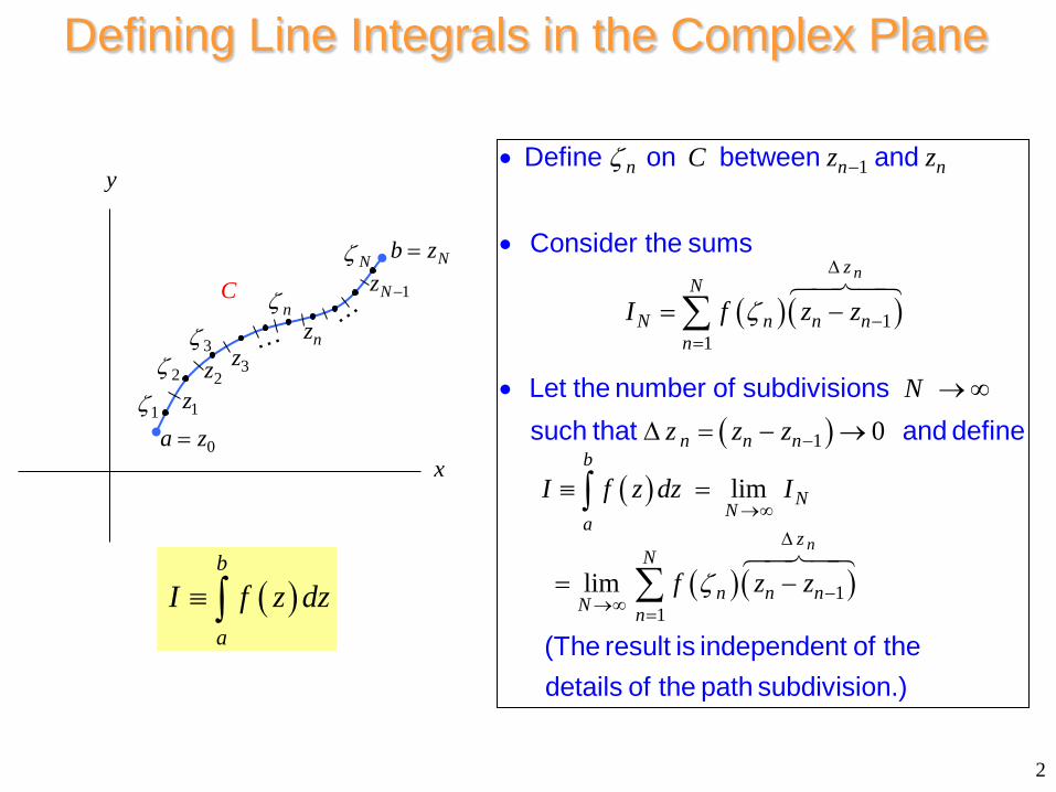
Defining Line Integrals in the Complex Plane

0a z=

Nb z=

1z2z

1ζ

3z2ζ

3ζ

Nζ1Nz −C

nznζ

x

y

( ) ( )

( )

( )

( ) ( )

1

11

1

11

0

lim

lim

n

n

n n n

zN

N n n nn

n n nb

NNa

zN

n n nN n

C z z

I f z z

Nz z z

I f z dz I

f z z

ζ

ζ

ζ

−

∆

−=

−

→∞∆

−→∞ =

= −

→ ∞

∆

•

•

= − →

=

= −

•

≡

∑

∫

∑

Define on between and

Consider the sums

Let the number of subdivisions such that and define

(The result is independent of the details of the path subdivision.)

2

( )b

a

I f z dz≡ ∫

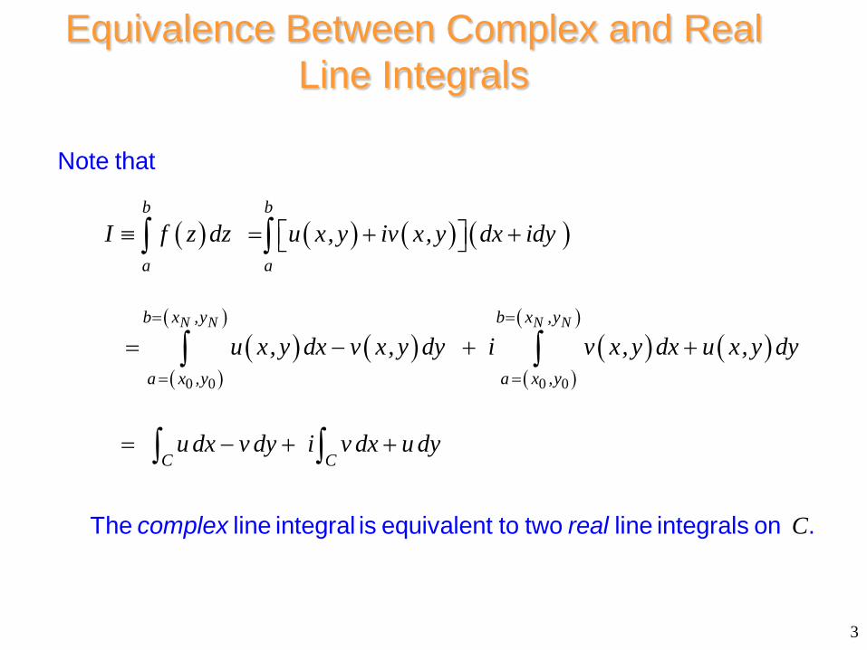
Equivalence Between Complex and Real Line Integrals

( ) ( ) ( ) ( )

( ) ( )( )

( )( ) ( )

( )

( )

0 0 0 0

N N N N

b b

a a

b x ,y b x ,y

a x ,y a x ,y

C C

I f z dz u x, y iv x, y dx idy

u x, y dx v x, y dy i v x, y dx u x, y dy

u dx v dy i v dx u dy

C

= =

= =

≡ = + +

= − + +

= − + +

∫ ∫

∫ ∫

∫ ∫

Note that

The line integral is equivalent to two line integrals on .complex real

3

Review of Line Integral Evaluation

( ) ( )

( ) ( )

0

0

f

C

t

t

f

u x, y dx v x, y dy

dx dyu v dtdt dt

C

C : x x t , y y t , t t t

t

−

−

= = ≤ ≤

∫

∫

A line integral written as

is really a shorthand for

where is some parameterization of :

t

t -a a

t -a a

1t2t 3t

1Nt −C

nt

x

y

0t

f Nt t=

( )( ), ( )x t y t

1t 2t 3t 1Nt −nt… … 0t f Nt t=

t

2 2 2

2 20

2 20

cos sin 0 2

f

f

x y a

x a t, y a t, t

x t , y a t , t a, t a,

x t , y a t , t a, t a,

θ π

◊ + =

= = ≤ = ≤

= = − = = −

= = − − = − =

parameterizations of the circle

1) (

Examp

)

2)

l

and

e :

4

The path C goes counterclockwise around the circle.

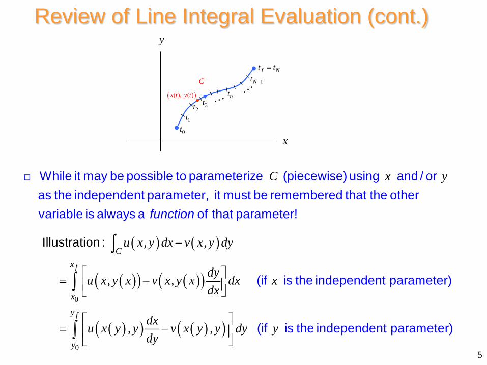
Review of Line Integral Evaluation (cont.)

C x y While it may be possible to parameterize (piecewise) using and / or as the independent parameter, it must be remembered that the other variable is always a of that parameter!

Illustra

function

( ) ( )

( )( ) ( )( )

( )( ) ( )( )

0

0

f

f

Cx

x

y

y

u x, y dx v x, y dy

dyu x, y x v x, y x dx xdx

dxu x y , y v x y , y dy ydy

−

= −

= −

∫

∫

∫

(if is the independent parameter)

(if is the independent paramet

tion :

er)

1t2t 3t

1Nt −C

nt

x

y

0t

f Nt t=

( )( ), ( )x t y t

5

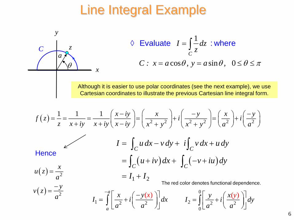
Line Integral Example

1

cos sin 0C

I dzz

C : x a , y a ,θ θ θ π

=◊

= = ≤ ≤

∫Evaluate : where

( ) 2 2 2 2 2 21 1 1 x iy x y x yf z i iz x iy x iy x iy x y x y a a

− − − = = = = + = + + + − + +

Although it is easier to use polar coordinates (see the next example), we use Cartesian coordinates to illustrate the previous Cartesian line integral form.

Consider

x

y

C

θa

z

( )

( )

2

2

xu zayv z

a

=

−=

Hence

1 2 2( )a

a

xx yI i dxa a

− − = + ∫

( ) ( )

1 2

C C

C C

I u dx v dy i v dx u dy

u iv dx v iu dy

I I

= − + +

= + + − +

= +

∫ ∫∫ ∫

0

2 2 20

( )y xI i dyya a

= + ∫

6

The red color denotes functional dependence.

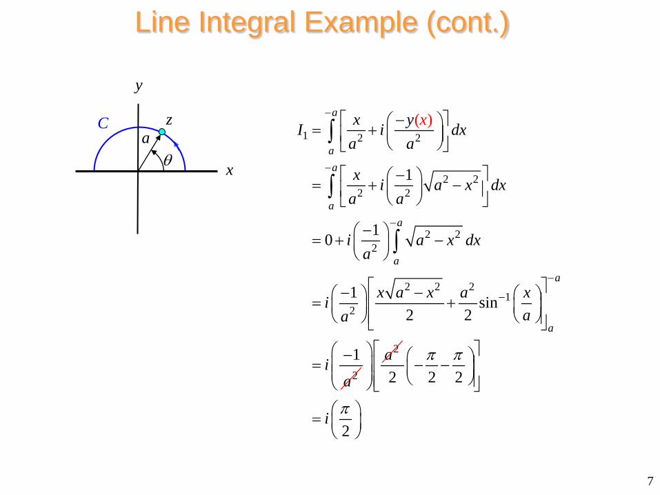
Line Integral Example (cont.)

Consider

x

y

C

θa

z1 2 2

2 22 2

2 22

2 2 21

2

2

1

10

1 sin2 2

1

( )a

aa

aa

aa

a

x yI i dxa a

x i a x dxa a

i a x dxa

x a x a xiaa

x

ia

−

−

−

−

−

− = +

− = + −

− = + −

− − = +

−=

∫

∫

∫

2a 2 2 2

2i

π π

π

− −

=

7

Line Integral Example (cont.)

Consider

x

y

C

θa

z

( )

0

2 2 20

0

20

02 2 2 2

2 20

2 22

0

2 2 21

2

0 2 2

0

( )

( )0

2

2 sin2 2

2

a

aa

a

y xI i dya a

i x dya

i ia y dy a y dya a

i a y dya

y a yi aa

y

ya

y

θ π π θ π

−

≤ ≤ ≤ ≤

= +

= +

= − + − −

= −

− = +

=

∫

∫

∫ ∫

∫

2

i

a

2a2

1sin

2

aa

i π

−

=

8

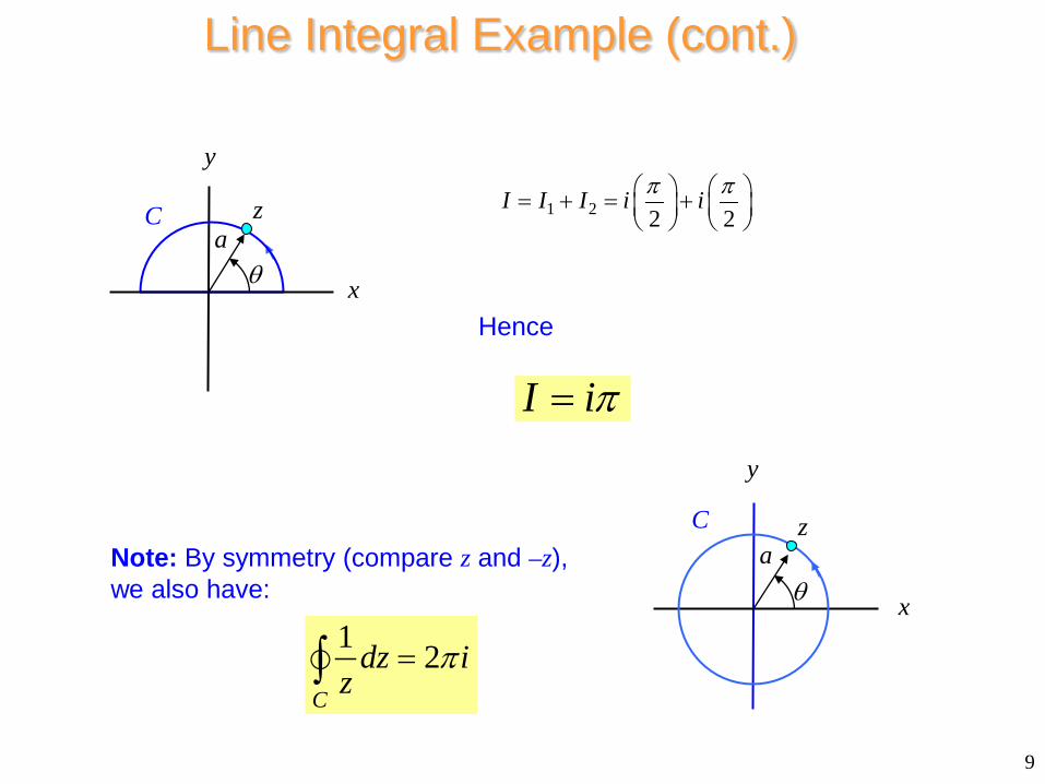
Line Integral Example (cont.)

Consider

x

y

C

θa

z 1 2 2 2I I I i iπ π = + = +

I iπ=

Hence

Note: By symmetry (compare z and –z), we also have:

1 2C

dz iz

π=∫x

y

C

θa

z

9

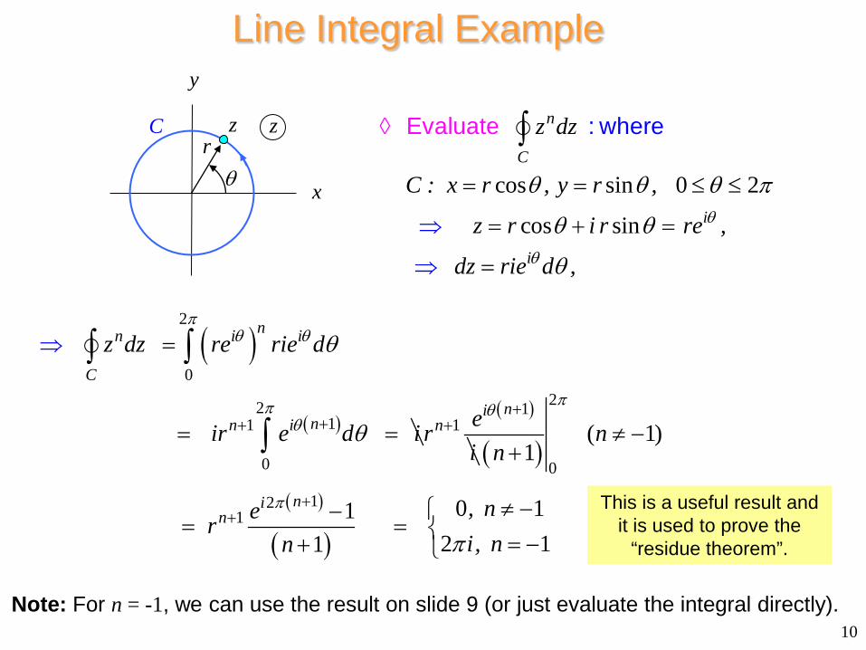
Line Integral Example

Consider

x

y

C

θr

z z

cos sin 0 2

cos sin

n

C

i

i

z dz

C : x r , y r ,

z r i r re ,

dz rie d ,

θ

θ

θ θ θ π

θ θ

θ

= = ≤ ≤

= + =

=

⇒

⇒

◊ ∫Evalua : where

te

( )

( )

2

0

211

0

nn i i

C

nn i

z dz re rie d

ir e d i

πθ θ

πθ

θ

θ++=

⇒ =

=

∫ ∫

∫

( )11

nin er

i

θ ++

( )( )

( )

2

0

121

( 1)1

0 112 11

nin

nn

, neri, nn

π

π

π

++

≠ −+

≠ −−= = = −+

This is a useful result and it is used to prove the

“residue theorem”.

10 Note: For n = -1, we can use the result on slide 9 (or just evaluate the integral directly).

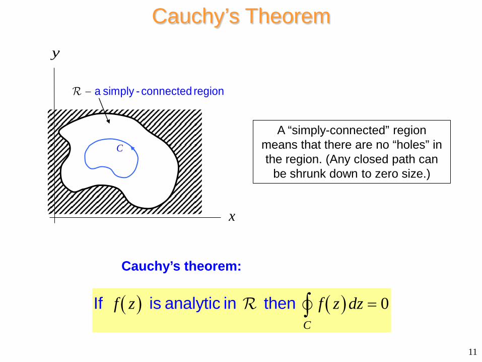
Cauchy’s Theorem

Consider

x

y

C

− a simply - connected region

( ) ( ) 0C

f z f z dz =∫If is analytic in then

11

A “simply-connected” region means that there are no “holes” in the region. (Any closed path can

be shrunk down to zero size.)

Cauchy’s theorem:

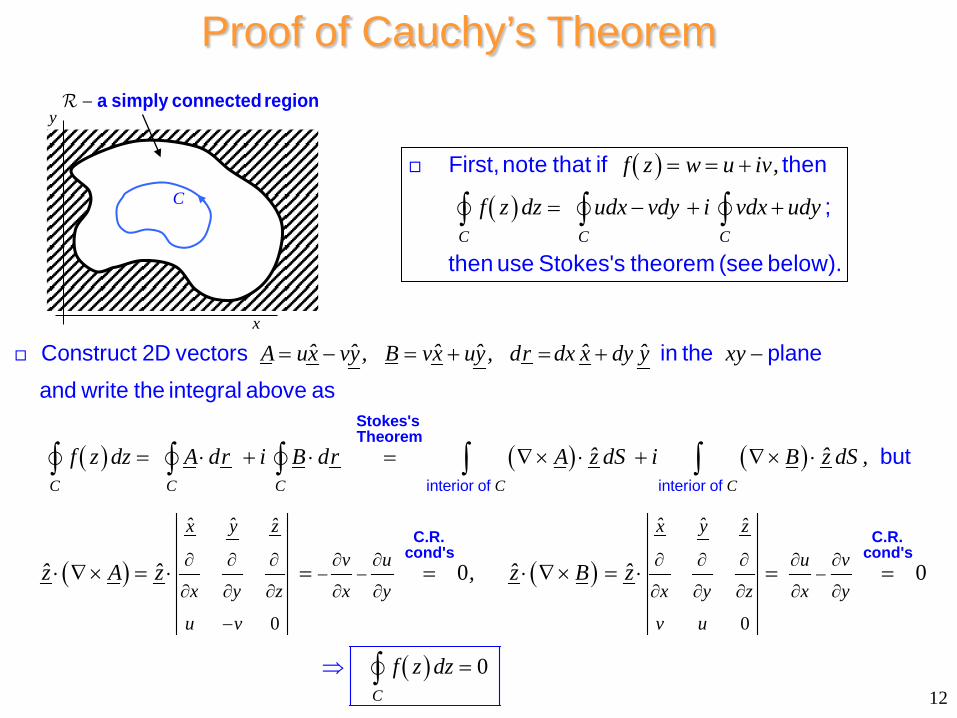
Proof of Cauchy’s Theorem

x

y

C

− a simply connected region

( )( )

C C C

f z w u iv,

f z dz udx vdy i vdx udy

= = +

= − + +∫ ∫ ∫

First, note that if then

;

then use Stokes's theorem (see below).

( ) ( ) ( )

( )

C C C C C

ˆ ˆ ˆ ˆ ˆ ˆA ux vy, B vx uy, dr dx x dy y xy

ˆ ˆf z dz A dr i B dr A z dS i B z dS ,

z A

= − = + = + −

= ⋅ + ⋅ = ∇ × ⋅ + ∇ × ⋅

⋅ ∇ ×

∫ ∫ ∫ ∫ ∫

interior of interior of

Construct 2D vectors in the plane and write the integral above as

but

Stokes's Theorem

( )

( )

0 0

0 0

0C

ˆ ˆ ˆ ˆˆ ˆx y z x y z

v u u v

x y z x y x y z x y

u v v u

ˆ ˆ ˆz , z B z

f z dz

∂ ∂ ∂ ∂ ∂ ∂ ∂ ∂ ∂ ∂− − −

∂ ∂ ∂ ∂ ∂ ∂ ∂ ∂ ∂ ∂

−

= ⋅ = = ⋅ ∇ × = ⋅ =

⇒

=

=∫

C.R. C.R.cond's cond's

12

Proof of Cauchy’s Theorem (cont.)

( ) ( )u x, y ,v x, yC

•

•

The proof using Stokes's theorem requires that have continuous first derivatives and that be smooth .

The Goursat proof removes these restrictions; hence the theorem is often called the .Cauchy -Goursat theorem

13

Some comments:

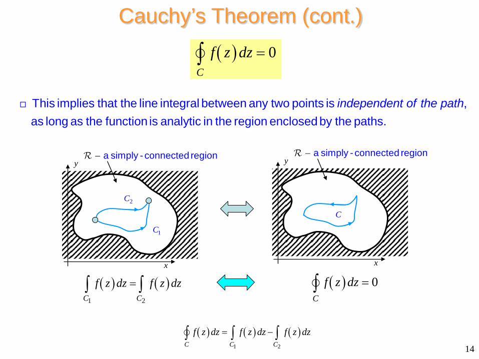
Cauchy’s Theorem (cont.)

Consider ( ) 0

C

f z dz =∫

This implies that the line integral between any two points is ,as long as the function is analytic in the region enclosed by the paths.

independent of the path

x

y

1C

− a simply - connected region

2C

( ) 0C

f z dz =∫( ) ( )1 2C C

f z dz f z dz=∫ ∫x

y

C

− a simply - connected region

14

( ) ( ) ( )1 2C C C

f z dz f z dz f z dz= −∫ ∫ ∫

Extension of Cauchy’s Theorem to Multiply-Connected Regions

( ) ( )

( )

1 2

1 2 1

0,C

C C c

f z f z dz

f z− +

•

•

≠

′

∫If is analytic in then in general.

Introduce an infinitesimal - width "bridge" to make into a simply connected region

2c+

( ) ( )

( ) ( )1 2

1 2

1 20C C

C C

dz f z dz f z dz c , c

f z dz f z dz⇒

= − =

=

∫ ∫ ∫

∫ ∫

since integrals along are in

opposite directions and thus cancel

Unlike in Cauchy's theorem, now integrals are usually nonvanishing!

x

y′ −simply - connected region

1C2C

1c2c

x

y− a multiply - connected region

1C2C

15

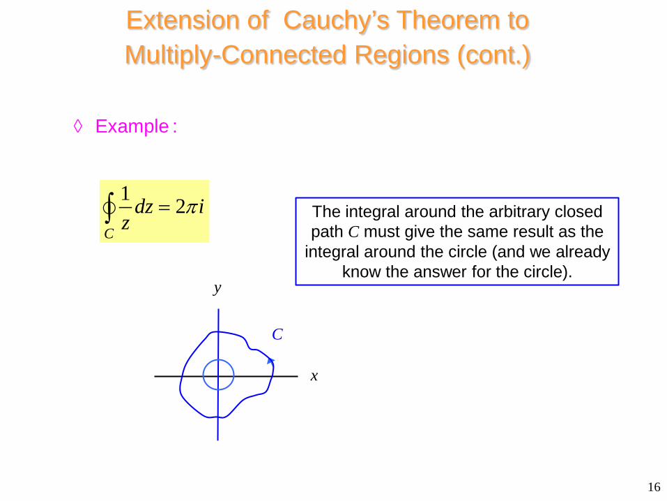
Extension of Cauchy’s Theorem to Multiply-Connected Regions (cont.)

16

◊ Example :

1 2C

dz iz

π=∫

x

y

C

The integral around the arbitrary closed path C must give the same result as the

integral around the circle (and we already know the answer for the circle).

Cauchy’s Theorem, Revisited

Consider

x

y

C

− a simply - connected region

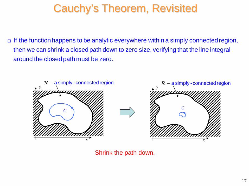
If the function happens to be analytic everywhere within a simply connected region, then we can shrink a closed path down to zero size, verifying that the line integral around the closed path must be zero.

x

y

C

− a simply - connected region

Shrink the path down.

17

Fundamental Theorem of the Calculus of Complex Variables

Consider

az

bz

1z2z 3z

1Nz −C

nz

x

y

1z∆2z∆

3z∆

Nz∆

18

( ) ( ) ( )

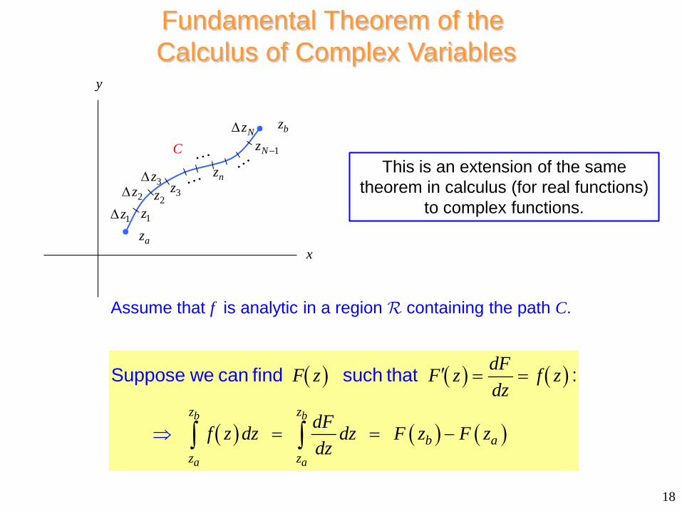
( ) ( ) ( )b b

a a

z z

b az z

dFF z F z f zdz

dFf z dz dz F z F zdz

′ = =

= = −⇒ ∫ ∫

Suppose we can find such that :

This is an extension of the same theorem in calculus (for real functions)

to complex functions.

Assume that f is analytic in a region containing the path C.

Fundamental Theorem of the Calculus of Complex Variables (cont.)

( )

( ) ( ) 11

1

lim

b

a

b

a

z

z

z N

n n n n nN nz

n n n

f R

f z dz

f z dz f z , z z z ,

C z z

ζ

ζ

−→∞ =

−

≡ ∆• ∆ −

•

=

∫

∑∫

is path independent in a simply

connected region (true if is analytic in ).

on between and (definition of line integr .

al)

Consider

az

bz

1z2z 3z

1Nz −C

nz

x

y

1z∆2z∆

3z∆

Nz∆

19

Starting assumptions:

( ) a bf z z z The integal is path independentif is analytic on paths from o . t

Recall :

Proof

Fundamental Theorem of the Calculus of Complex Variables (cont.)

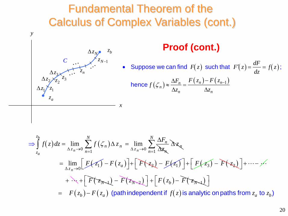
( ) ( )0 01

lim limb

n na

z Nn

n nz z nnz

Ff z dz f zz

ζ∆ → ∆ →=

∆= ∆ =⇒

∆∑∫ nz∆

( )1

10lim

n

N

n

zF z

=

∆ →=

∑

( ) ( )2aF z F z − + ( )1F z− ( )3F z + ( )2F z− + −

+ ( )1NF z −+ ( )2NF z −− ( ) ( )1b NF z F z − + − ( ) ( ) ( )b a a bF z F z f z z z

= − (path independent if is analytic on paths from to )

Consider

az

bz

1z2z 3z

1Nz −C

nz

x

y

1z∆2z∆

3z∆

Nz∆

20

( ) ( ) ( )

( ) ( ) ( )1n nnn

n n

dFF z F z f zdz

F z F zFfz z

ζ −

′ = =

−∆≈ =

∆ ∆

• Suppose we can find such that ;

hence

Proof (cont.)

Fundamental Theorem of the Calculus of Complex Variables (cont.)

( ) ( ) ( )

1sin cos

1

b

a

z

b az

n azn az

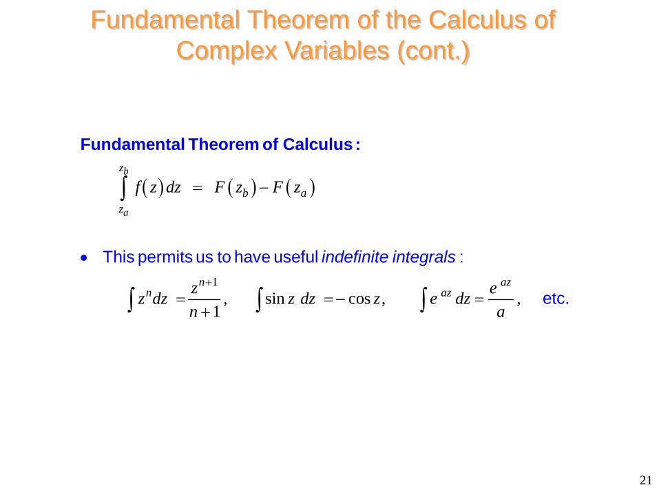
f z dz F z F z

z ez dz , z dz z, e dz ,n a

+

= −

= = − =

•

+

∫

∫ ∫ ∫

This permits us to have useful :

etc.

Fundamental Theorem of Calculus :

indefinite integrals

21

Fundamental Theorem of the Calculus of Complex Variables (cont.)

( ) ( ) ( )

( ) ( ) ( )

( ) ( ) ( ) ( ) ( )

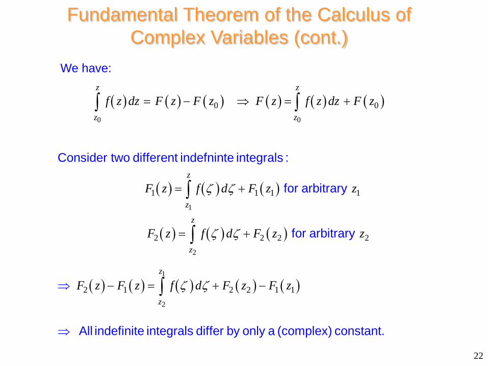
1

2

1

2

1 1 1 1

2 2 2 2

2 1 2 2 1 1

z

z

z

z

z

z

F z f d F z z

F z f d F z z

F z F z f d F z F z

ζ ζ

ζ ζ

ζ ζ

= +

= +

= +

⇒

−⇒ −

∫

∫

∫

Consider two different indefninte integrals :

for arbitrary

for arbitrary

All indefinite integrals differ by only a (complex) constant.

22

( ) ( ) ( ) ( ) ( ) ( )0 0

0 0

z z

z z

f z dz F z F z F z f z dz F z= − ⇒ = +∫ ∫

We have:

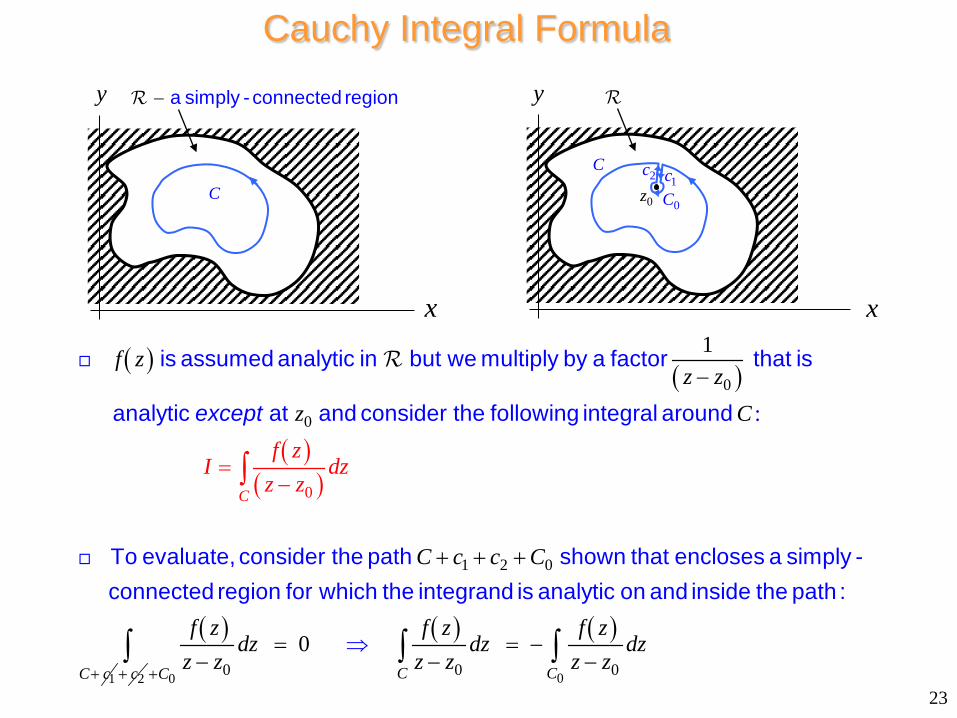
Cauchy Integral Formula

( ) ( )

( )( )

0

0

1 2 0

0

:

1

C

f zz z

z Cf z

I dz

C

z z

C c c

−

+ + +

=−∫

is assumed analytic in but we multiply by a factor that is

analytic at and consider the following integral around

To evaluate

, consider the path shown that

except

( )

1 0C c

f zdz

z z+

−

encloses a simply - connected region for which the integrand is analytic on and inside the path :

2c+

( ) ( )

00 0 00

C CC

f z f zdz dz

z z z z+

= = −− −

⇒∫ ∫ ∫

x

y

C

− a simply - connected region

23

x

y

C

0z0C

1c2c

Cauchy Integral Formula (cont.)

( )( ) ( )

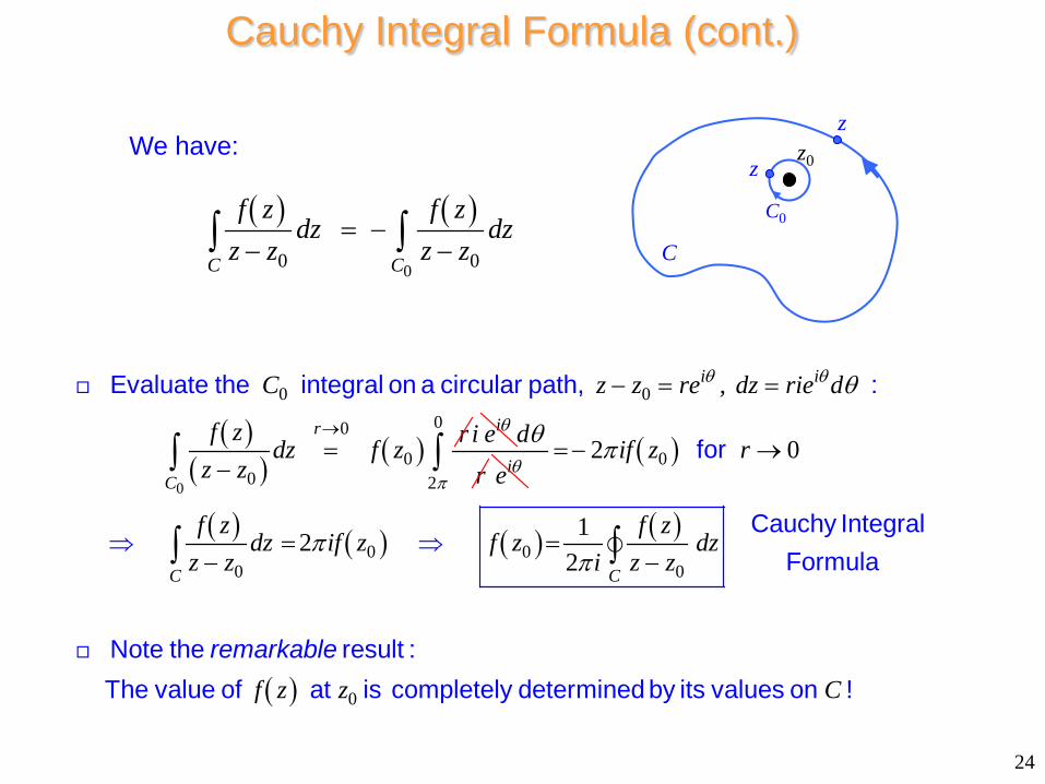
0

0 0

0

00

i i

r

C

C z z re , dz rie d

f z rdz f zz z

θ θ θ→

− = =

=−∫

Evaluate the integral on a circular path, :ii e θ d

rθ

ie θ( )

( ) ( ) ( ) ( )

( )

0

02

0 00 0

0

2 0

122C C

if z r

f z f zdz if z f z dz

z z i z z

f z z C

π

π

ππ

= −

=−

⇒−

⇒

→

=

∫

∫ ∫

for

Cauchy IntegralFormula

Note the result :

The value of at is completely determined by its values on ! remarkable

( ) ( )

00 0C C

f z f zdz dz

z z z z= −

− −∫ ∫

0z

0C

C

z

z

24

We have:

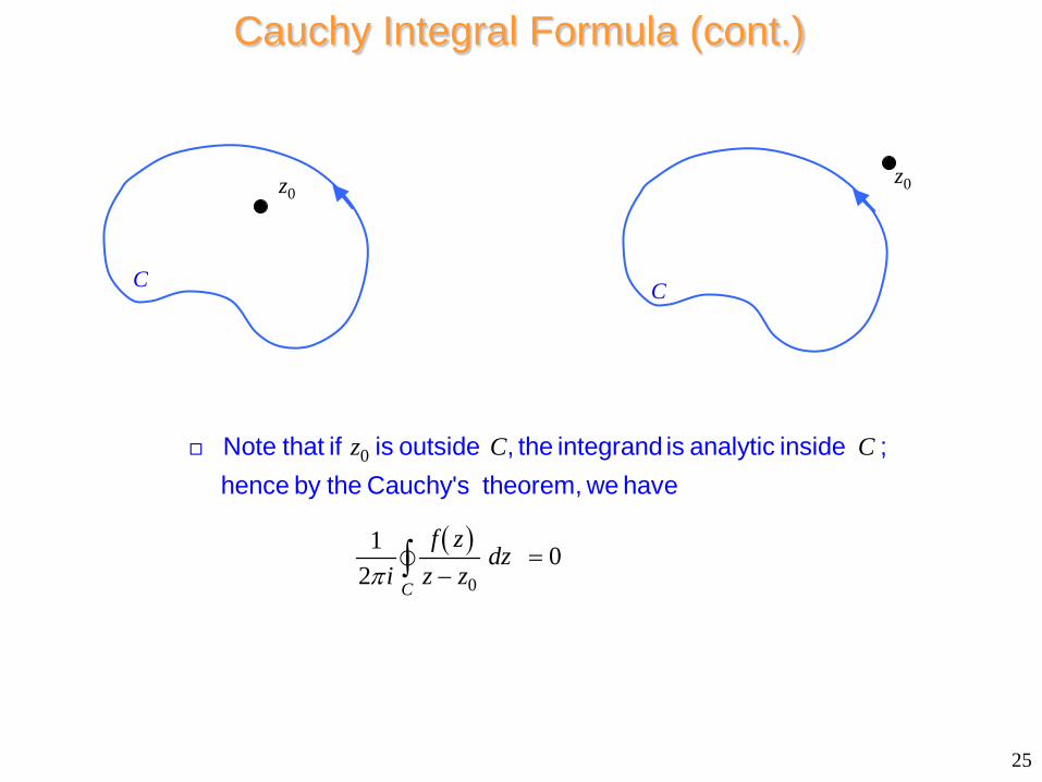
Cauchy Integral Formula (cont.)

( )

0

0

1 02 C

z C C

f zdz

i z zπ=

−∫

Note that if is outside , the integrand is analytic inside ; hence by the Cauchy's theorem, we have

0z

C

0z

C

25

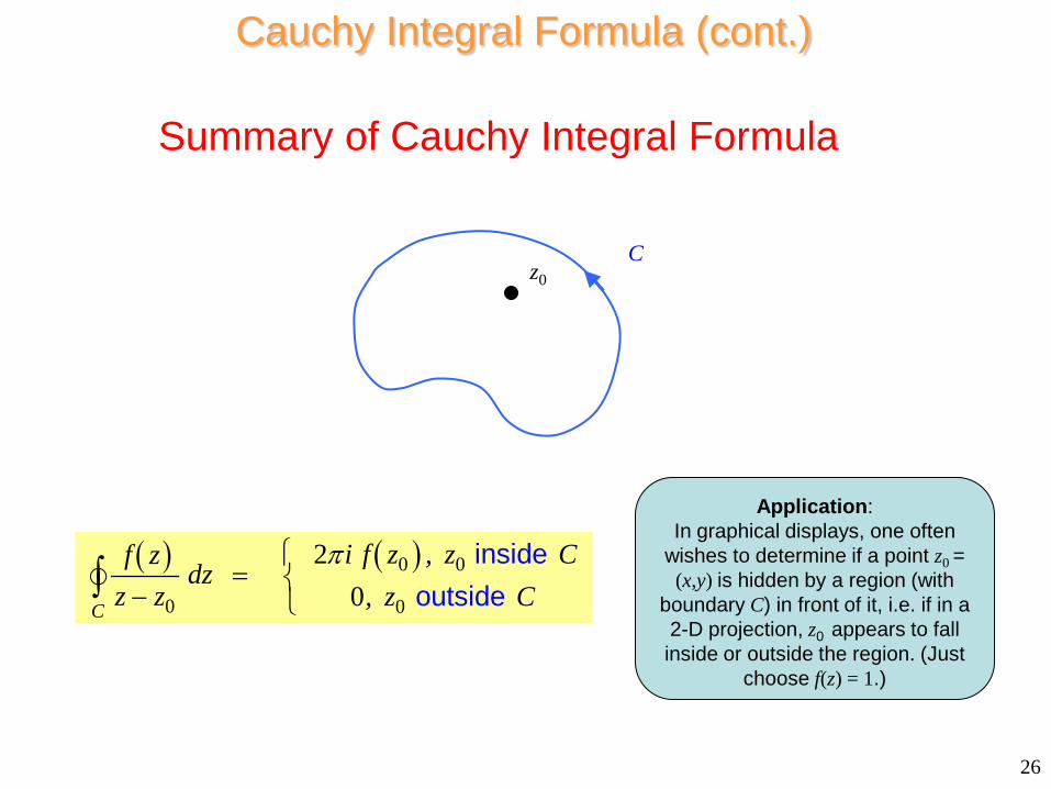
Cauchy Integral Formula (cont.)

( ) ( )0 0

0 0

20C

i f z , z Cf zdz

z z , z Cπ

= − ∫

inside outside

0zC

Application: In graphical displays, one often

wishes to determine if a point z0 = (x,y) is hidden by a region (with

boundary C) in front of it, i.e. if in a 2-D projection, z0 appears to fall inside or outside the region. (Just

choose f(z) = 1.)

26

Summary of Cauchy Integral Formula

Derivative Formulas

( ) ( )

( ) ( ) ( ) ( )

00

0 0

0 0

12

12

12

C

C

f zf z z dz

i z z z

f z z f z f z f zdz

z i z z z z z z

i z

π

π

π

+ ∆ =− − ∆

+ ∆ − ⇒

= − ∆ ∆ − − ∆ −

=∆

∫

∫

( ) zf z ∆( )( )

( ) ( ) ( ) ( ) ( )

( ) ( )( )

0 0

0 00 0 0 0

0 200

1 1lim lim2

12

C

z zC

C

dzz z z z z

f z z f zf z dz

z i z z z z z

f zf z dz

zi z .z

π

π

∆ → ∆ →

− − ∆ −

+ ∆ −= ∆ − − ∆ −

′ =−

⇒

⇒

∫

∫

∫

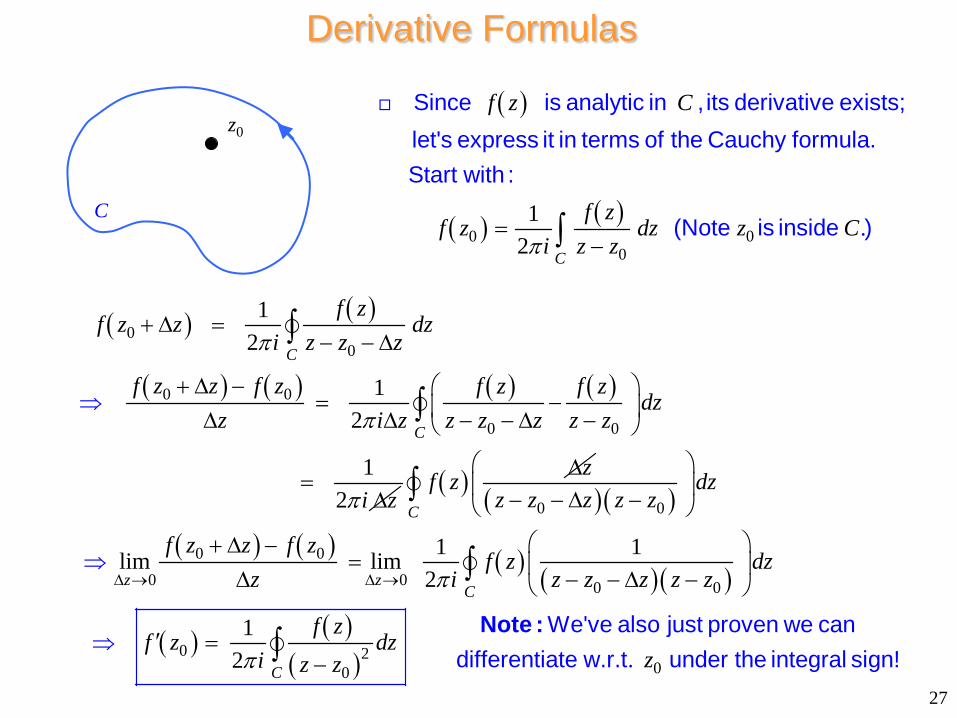
We've also just proven we can differentiate w.r.t under the integral sign!

Note :

0z

C

( )

( ) ( )0 0

0

12 C

f z C

f zf z dz z C

i.

z zπ=

−∫

Since is analytic in , its derivative exists;let's express it in terms of the Cauchy formula.Start with :

(Note is inside )

27

Derivative Formulas (cont.)

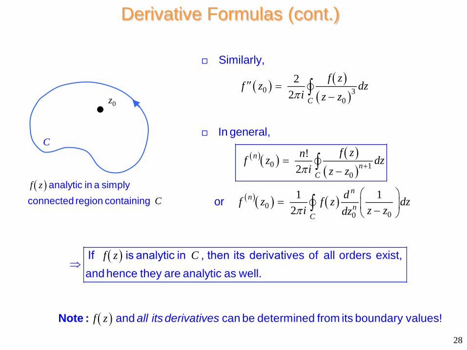
( )f z C⇒

Ιf is analytic in , then its derivatives of all orders exist, and hence they are analytic as well.

0z

C

( ) ( )( )

( )( ) ( )( )

( )( ) ( )

0 30

0 10

000

22

!2

1 12

C

nn

C

nn

nC

f zf z dz

i z z

f znf z dzi z z

df z f z dzi z zdz

π

π

π

+

′′ =−

=−

= −

∫

∫

∫

Similarly,

In general,

or( )f z

C analytic in a simply

connected region containing

( )f z and can be determined from its boundary values! Note : all its derivatives

28

Morera’s Theorem

( ) ( ) ( ) ( )

( ) ( )

0

0

0z

C z

f z dz f z F z f d .

F z F z

ζ ζ

−

⇒= ≡∫ ∫

is path independent, so define

Note that

Proof

( ) ( ) ( ) ( ) ( )

( ) ( )

0 0

0

0 0

0

z z

z z

F z F z fF z f d

f

, dz z z z

F z F zz

ζζ ζ ζ

−= = =

− −

−

∫ ∫and

We can chose a small straight - line path between the two points since the integral is path independent. Along this small path, is almost constant.Note :

( ) ( )0

0

0

0 0 0

z z z

z

f zfd

z z z z zζ

ζ→

= →− − −∫ ( )0z z− ( )0

0

0

f z f

F z F f .f z

⇒

=

′ =

(from continuity of ).

is analytic at any in . But then so are all its derivatives, including Hence, is analytic at .

( )

( )

( )

0C

f z

f z dz

C f z

=∫

Ιf a function is continuous in a simply - connectedregion and

for closed contour within , then is analytic throughout .

every

F will be analytic if we can prove its derivative exists!

0z

zζ

29

Comparing Cauchy’s and Morera’s Theorems

( )

( )

( )( )

0

0

C

C

f z

f z dz C

f z

f z dz

=

=

•

•

∫

∫

Cauchy's Theorem : If is analytic in a simply - connected region then

, in .

Morera's Theorem : Ιf a function is continuous in a simply -

connected region and for

( )C f z

•

every closed contour

within , then is analytic throughout .

These theorems are converses of one another!

30

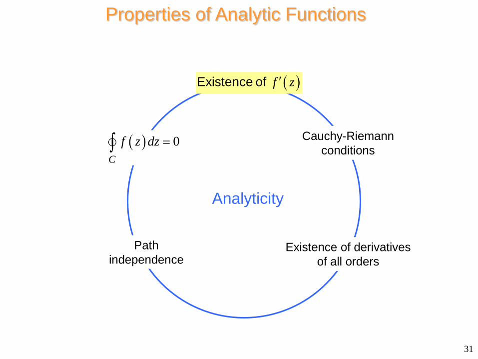
Properties of Analytic Functions

Analyticity

Cauchy-Riemann conditions ( ) 0

Cf z dz =∫

Path independence

( )f z′Existence of

31

Existence of derivatives of all orders

Cauchy’s Inequality

( ) ( )

( )0

nn

n

n n

f z f z M

f z a z

MR a .R

∞

=

<

=

≤

∑

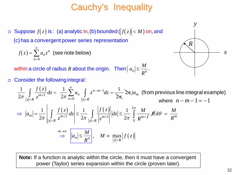
Suppose is : (a) analytic , (b) bounded ( ) , and

(c) has a convergent power series representation

a circle of radius about the origin

(see note below

. Then

in on

withi

n

)

C

( ) 11

0

1 1 12 2 2

n mnm

nz R z R

f zdz a z dz

zπ π π

∞− −

+== =

= =∑∫ ∫

onsider the following integral :

2π

( ) ( )1 1 1

1 1 12 2 2

m

m m m mz R z R

ia

f zf z Ma dz dzz z Rπ π π+ + +

= =

=⇒ ≤ ≤∫ ∫

(from previous line integral example)

R

( )

2

0

max

m

m n

n n z R

MdR

Ma , M f zR

π

θ

→

=

=

≡⇒ ≤

∫

Note: If a function is analytic within the circle, then it must have a convergent power (Taylor) series expansion within the circle (proven later).

32

1 1n m− − = −where

x

y

R

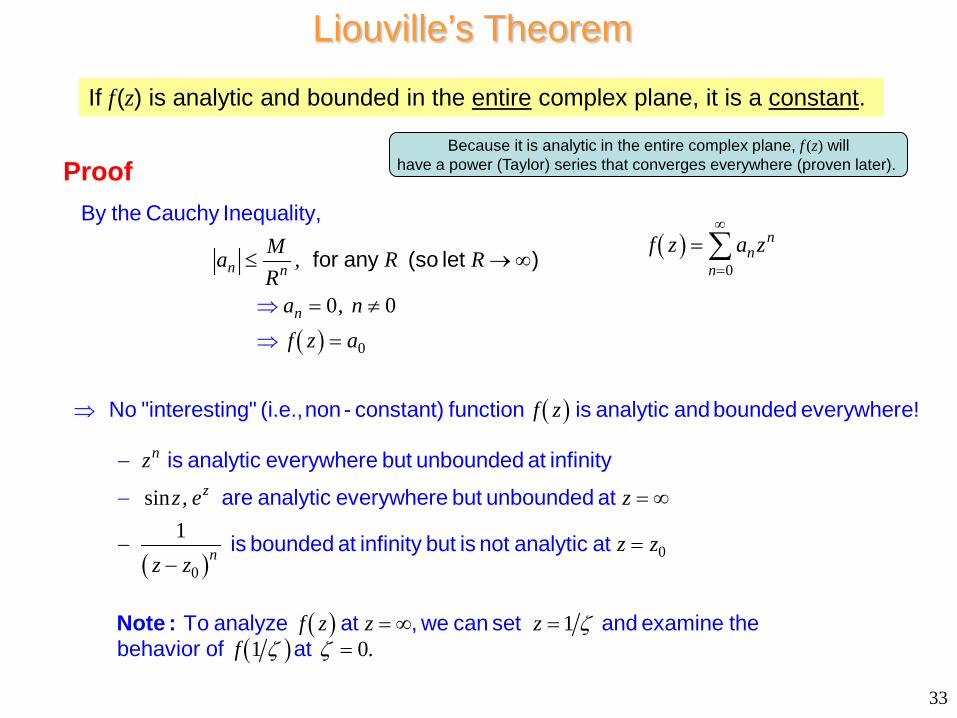
Liouville’s Theorem

( )

( )

0

0 0

n n

n

n

Ma , R RR

a , nf z a

f z

z

⇒

⇒

≤ → ∞

=

−

≠

=

⇒

By the Cauchy Inequality,

No "interesting" (i.e., non - constant) function is analytic and bounded everywhere!

is analytic everywhere

for a

but u

ny (so let )

nbounded at

( )

( )( )

00

sin1

11 0

z

n

z, e z

z zz z

f z z zf .

ζζ ζ

= ∞

=−

==

−

∞ =

−

infinity

are analytic everywhere but unbounded at

is bounded at infinity but is not analytic at

To analyze at , we can set and examine the behavior of at Note :

Because it is analytic in the entire complex plane, f (z) will have a power (Taylor) series that converges everywhere (proven later).

( )0

nn

nf z a z

∞

== ∑

33

Proof

If f (z) is analytic and bounded in the entire complex plane, it is a constant.

The Fundamental Theorem of Algebra

(This theorem is due to Gauss*.)

Carl Friedrich Gauss

( ) ( )( ) ( )1 2N N NP z a z z z z z z= − − −

As a corollary, an Nth degree polynomial can be written in factored form as

* The theorem was first proven in Gauss’s doctoral dissertation in 1799 using an algebraic method. The present proof, based on Liouville’s theorem, was given by him later, in 1816.

(his signature) http://en.wikipedia.org/wiki/Carl_Friedrich_Gauss

34

( )0

0 0N

nN n N

nN P z a z , a , N , N

== ≠ >∑The th degree polynomial, has (complex) roots.

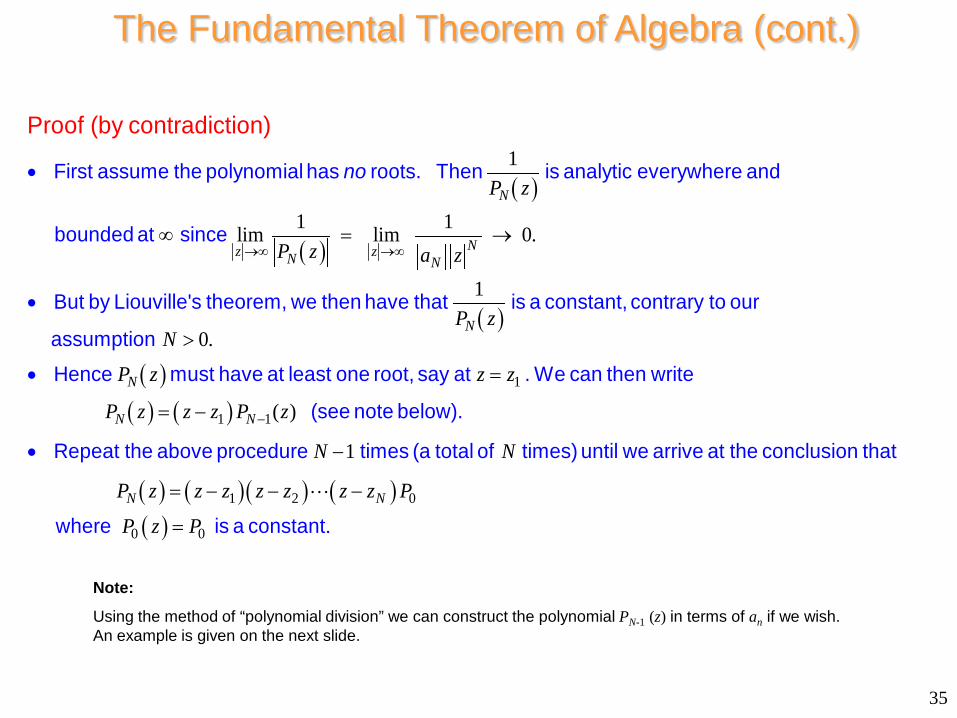
The Fundamental Theorem of Algebra (cont.)

( )

( )

1

1 1lim lim 0

1

N

Nz zN N

N

P z

.P z a z

P

→∞ →∞∞ =

•

→

• First assume the polynomial has roots. Then is analytic everywhere and

bounded at since

But by Liouville's theorem, we then have that

Proof (by contradiction)

no

( )

( )( ) ( )

1

1 1

0

( )

1

N

N N

zN .

P z z z

P z z z P z

N−

•

>

=

•

= −

−

is a constant, contrary to our

assumption

Hence must have at least one root, say at . We can then write

(see note below).

Repeat the above procedure times (a total of

( ) ( )( ) ( )( )

1 2 0

0 0

N N

N

P z z z z z z z P

.P z P

= − − −

=

times) until we arrive at the conclus

ion that

where is a constant

Note:

Using the method of “polynomial division” we can construct the polynomial PN-1 (z) in terms of an if we wish. An example is given on the next slide.

35

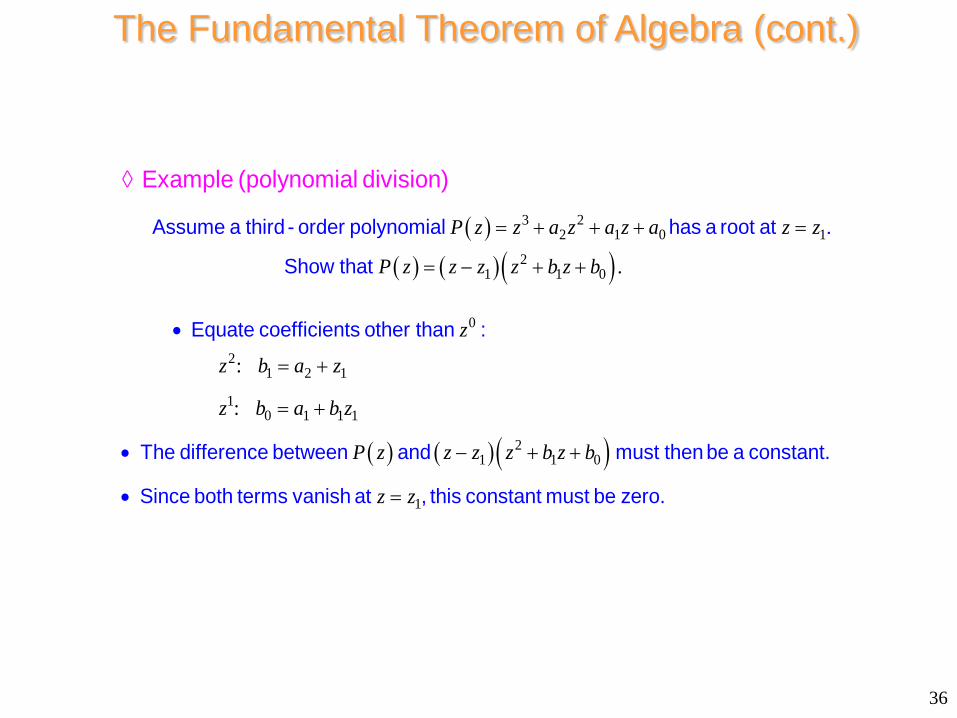
The Fundamental Theorem of Algebra (cont.)

( )( ) ( ) ( )

3 22 1 0 1

21 1 0

0

21 2 1

10 1 1 1

:

:

.P z z a z a z a z z

P z z z z b z b .

z

z b a z

z b a b z

= + + + =

= − + +

+

•

= +

•

=

◊

Assume a third - order polynomial has a root at

Show that

Equate coefficients other than :

The difference

Example (polynomial division)

( ) ( ) ( )21 1 0

1

P z z z z b z b

z z

− + +

=•

between and must then be a constant.

Since both terms vanish at , this constant must be zero.

36

Numerical Integration in the Complex Plane

37

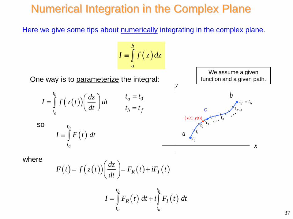
Here we give some tips about numerically integrating in the complex plane.

( )b

a

I f z dz≡ ∫

( )( )b

a

t

t

dzI f z t dtdt

= ∫

One way is to parameterize the integral:

( )b

a

t

t

I F t dt≡ ∫

where ( ) ( )( ) ( ) ( )R I

dzF t f z t F t iF tdt

= = +

so

( ) ( )b b

a a

t t

R It t

I F t dt i F t dt= +∫ ∫

1t2t 3t

1Nt −C

nt

x

y

0t

f Nt t=

( )( ), ( )x t y t

a

b

We assume a given function and a given path.

0a

b f

t tt t

=

=

Numerical Integration in the Complex Plane (cont.)

38

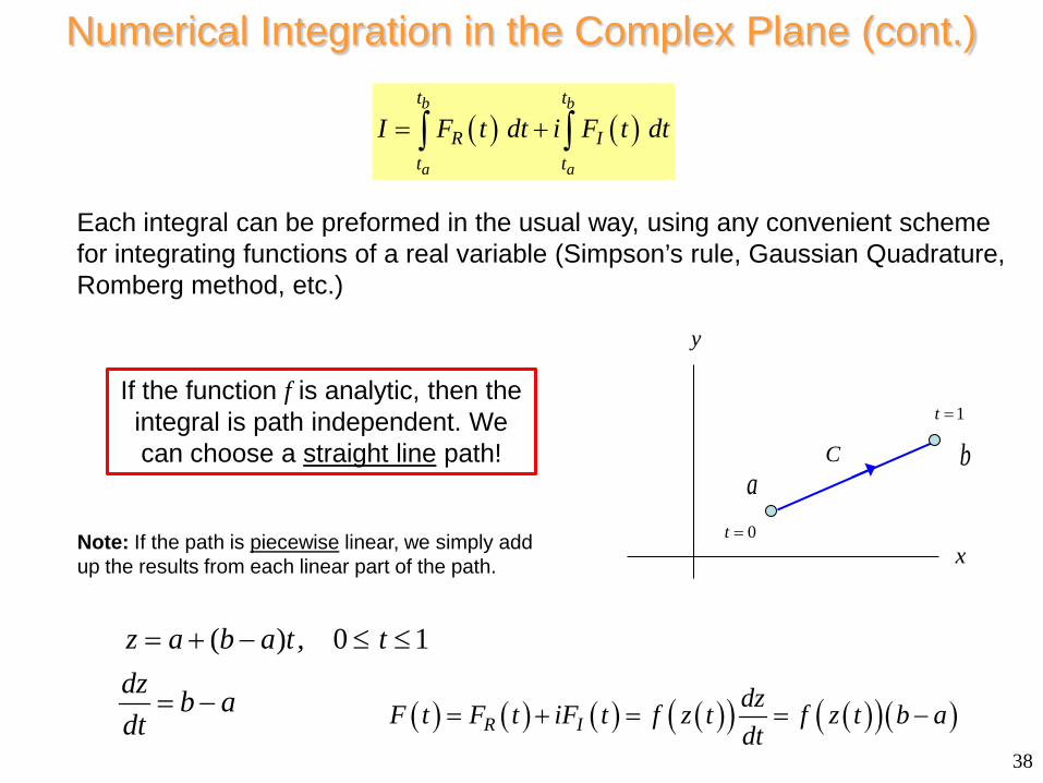
Each integral can be preformed in the usual way, using any convenient scheme for integrating functions of a real variable (Simpson’s rule, Gaussian Quadrature, Romberg method, etc.)

( ) ( )b b

a a

t t

R It t

I F t dt i F t dt= +∫ ∫

If the function f is analytic, then the integral is path independent. We can choose a straight line path!

x

y

0t =

1t =

Ca

b

( ) 0 1z a b a t , tdz b adt

= + − ≤ ≤

= −

Note: If the path is piecewise linear, we simply add up the results from each linear part of the path.

( ) ( ) ( ) ( )( ) ( )( )( )R IdzF t F t iF t f z t f z t b adt

= + = = −

39

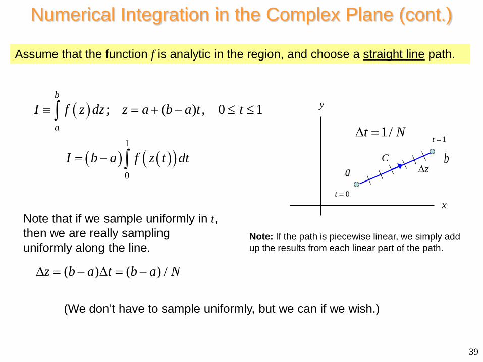
( ) ; ( ) 0 1b

a

I f z dz z a b a t , t≡ = + − ≤ ≤∫

( ) ( )( )1

0

I b a f z t dt= − ∫

Note that if we sample uniformly in t, then we are really sampling uniformly along the line.

( ) ( ) /z b a t b a N∆ = − ∆ = −

x

y

0t =

1t =

Ca

bz∆

(We don’t have to sample uniformly, but we can if we wish.)

Numerical Integration in the Complex Plane (cont.)

Assume that the function f is analytic in the region, and choose a straight line path.

Note: If the path is piecewise linear, we simply add up the results from each linear part of the path.

1/t N∆ =

40

( ) ( )( )1

0

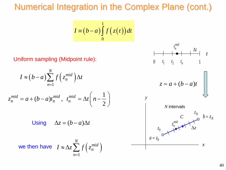
I b a f z t dt≡ − ∫

( )z b a t∆ = − ∆

Uniform sampling (Midpoint rule):

( ) ( )1

Nmidn

nI b a f z t

=≈ − ∆∑

1( )2

mid mid midn n nz a b a t , t t n = + − = ∆ −

Using

( )1

Nmidn

nI z f z

=≈ ∆ ∑

Numerical Integration in the Complex Plane (cont.)

x

y

C

0a z=

Nb z=

z∆midnz

0z

NzN intervals

we then have

t 0 1t 2t

t∆midnt

nt 1

( )z a b a t= + −

41

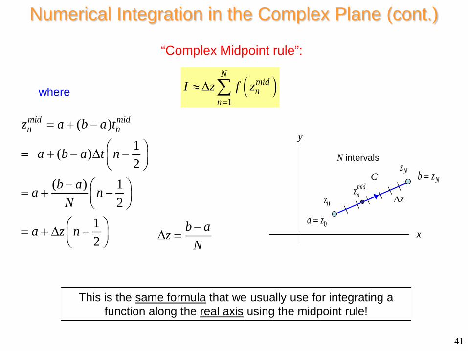
b azN−

∆ =

“Complex Midpoint rule”:

( )1

Nmidn

nI z f z

=

≈ ∆ ∑

This is the same formula that we usually use for integrating a function along the real axis using the midpoint rule!

Numerical Integration in the Complex Plane (cont.)

x

y

C

0a z=

Nb z=

z∆midnz

0z

NzN intervals

where

( )1( )2

( ) 12

12

mid midn nz a b a t

a b a t n

b aa nN

a z n

= + −

= + − ∆ −

− = + −

= + ∆ −

42

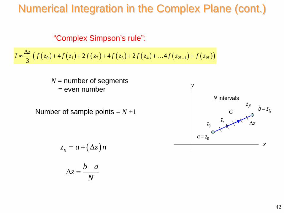
( ) ( ) ( ) ( ) ( ) ( ) ( )( )0 1 2 3 4 14 2 4 2 43 N NzI f z f z f z f z f z f z f z−

∆≈ + + + + + +

“Complex Simpson’s rule”:

N = number of segments = even number

( )nz a z n= + ∆

b azN−

∆ =

Numerical Integration in the Complex Plane (cont.)

x

y

C

0a z=

Nb z=

z∆nz0z

N intervals Nz

Number of sample points = N +1

43

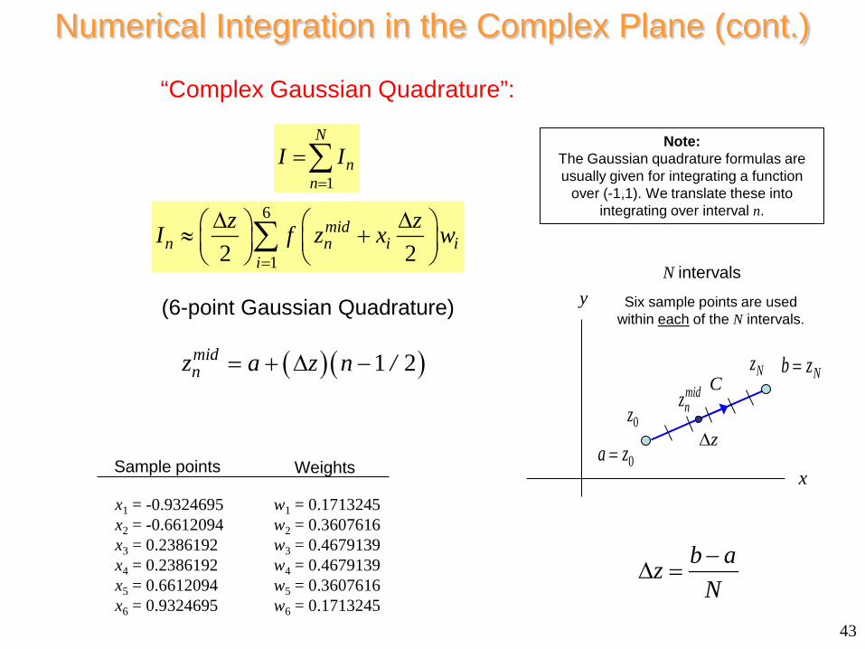
1

N

nn

I I=

=∑

“Complex Gaussian Quadrature”:

b azN−

∆ =

Numerical Integration in the Complex Plane (cont.)

6

12 2mid

n n i ii

z zI f z x w=

∆ ∆ ≈ +

∑

x1 = -0.9324695 x2 = -0.6612094 x3 = 0.2386192 x4 = 0.2386192 x5 = 0.6612094 x6 = 0.9324695

w1 = 0.1713245 w2 = 0.3607616 w3 = 0.4679139 w4 = 0.4679139 w5 = 0.3607616 w6 = 0.1713245

(6-point Gaussian Quadrature)

Sample points Weights

( ) ( )1 2midnz a z n /= + ∆ −

x

y

C

0a z=

Nb z=

z∆0z

Six sample points are used within each of the N intervals.

Nzmidnz

N intervals

Note: The Gaussian quadrature formulas are usually given for integrating a function

over (-1,1). We translate these into integrating over interval n.

44

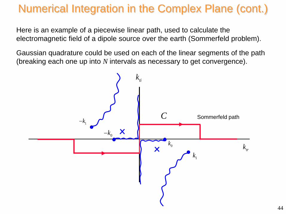
Numerical Integration in the Complex Plane (cont.)

Here is an example of a piecewise linear path, used to calculate the electromagnetic field of a dipole source over the earth (Sommerfeld problem).

Gaussian quadrature could be used on each of the linear segments of the path (breaking each one up into N intervals as necessary to get convergence).

tik

0k0−k

trk1k

1−kC Sommerfeld path