Embed Size (px)
Citation preview
G u n n & T w y n m o r e
An overview of commonly used royalty rate methodologies Hester Tak
January 15
08 Fall

2
Table of Contents
Foreword .............................................................................................................................. 3
Introduction ........................................................................................................................ 4
Chapter 1: Intellectual Property ................................................................................... 5 The Patent System ............................................................................................................................................. 5 Application of IP Valuation in recent years ............................................................................................ 6 Assignment versus Licenses ......................................................................................................................... 7 Chapter 2: Royalty and Royalty Models ..................................................................... 9 What is Royalty? ................................................................................................................................................. 9 Lump Sum .............................................................................................................................................................. 9 Minimum Royalty ............................................................................................................................................... 9 “Fixed Per-‐License” Royalty ........................................................................................................................... 9 Volume-‐ or Revenue-‐Based Royalty ........................................................................................................ 10 List-‐Based Royalty (LBR) ............................................................................................................................. 10 Net-‐Based Royalty (NBR) ............................................................................................................................. 10
Payments Prior to Royalty ........................................................................................................................... 11 When Are Royalty Rates Set? ...................................................................................................................... 11 Chapter 3. Valuation Models ....................................................................................... 12 Traditional Patent Valuation Methods ................................................................................................... 12 Cost Approach – Accounting for (Historical) Costs .......................................................................... 12 Market/Transactional Approach – Accounting for Market Conditions .................................. 13 Income approach – Accounting for Future Value ............................................................................. 13 25% Rule of Thumb .............................................................................................................................................. 14 DCF – Accounting for Time and Uncertainty .............................................................................................. 14
The More Complex Valuation Models ..................................................................................................... 14 Decision Tree Analysis – Accounting for Flexibility .......................................................................... 15 Option Pricing Model: Monte Carlo Simulation– Accounting for Riskiness (continuous time) ...................................................................................................................................................................... 15 Option Pricing Model: Binomial Tree – Accounting for Riskiness (Discrete Time) ............ 15
Hybrid Models ................................................................................................................................................... 16 Hybrid Model 1 (Institut Curie) ................................................................................................................. 17 Hybrid Model 2 (Syracuse University) .................................................................................................... 17 Hybrid Model 3 (VTT Technical Research Centre Finland) .......................................................... 19 Hybrid Model 4 (Boston College) .............................................................................................................. 20
Discussion & Conclusions ............................................................................................ 22 Alternative approaches ................................................................................................................................. 24 In summary ........................................................................................................................................................ 24 References ......................................................................................................................... 26
APPENDIX .......................................................................................................................... 29

3
Foreword This report is an adaptation of an academic chapter written by HS Tak for the Master in Business Valuation, September 2012.

4
Introduction The aim of this report is twofold: a) to investigate whether a logical process can be developed that can guide practitioners to select the most appropriate royalty structure and subsequently use an appropriate valuation methodology b) investigate if there are models that can be used to value IP regardless of the type of technology, type of market etc. The origin of the report lies in the observation that many practitioners seem to, almost randomly, mix certain royalty structures with clear underlying assumptions and traditional IP valuation methods with completely different underlying assumptions. It has also been observed that there is a growth in the various models used to value IP and determine a royalty rate. As with the traditional methods, there seems to be a lack of guidelines as to when to use the models. After a short introduction to IP in Chapter 1, the different royalty structures used most often in licenses are set out (Chapter 2). In Chapter 3, different valuation methods are looked at that are used to set a royalty rate. There are three different categories of models described in the report: traditional methods used to value IP in licenses, complex models available to value IP and hybrid models that have evolved by practitioners, some with an academic link to a University. In Chapter 4, the schematic process that practitioners can use is explained and applied to the hybrid models. The aim of this report is not to analyze the accurateness or logic of the hybrid models themselves but to relate them to the developed process. This should then give an idea when and how different models could be applied.

5
Chapter 1: Intellectual Property Intellectual Property (IP) refers to the form of expression of ideas and creations of the mind. As with real property, IP is an asset that can be sold, bought, licensed, exchanged or given away freely. The most obvious difference between the two is that IP is an intangible, and as such, cannot be identified by its own physical parameters. Therefore, these intangible assets must be expressed in such a way that it can be protected1 There are two “groups” that can be identified: industrial IP (trademarks, patents, design etc.) and copyright -‐ the latter being the most well known form of IP. Copyright deals with the rights of intellectual creators “in their creation” and is an automatic right that is granted by law, when the work is produced. In many cases, this would be when the creation takes a physical form such as a book or a painting. However, in some cases, the work is protected before it is written down such as a poem or a music tune.2 For industrial IP, on the other hand, protection needs to be sought actively, by means of a patent, after the IP has been reduced to a tangible form. A quick introduction to the patent system is given below.
The Patent System The principle behind today’s patent system is not new. In fact, the earliest form of a patent system dates back to 500 BC in the Greek city of Sybaris where "encouragement was held out to all who should discover any new refinement in luxury, the profits arising from which were secured to the inventor by patent for the space of a year." 3 The current patent system still serves the same purpose: it is designed to stimulate disclosure of inventions in exchange for the right to prevent others from commercially exploiting the same invention. The disclosure requirement is key as it is believed that the development of new innovative ideas and products is stimulated through this mechanism. In 1449, King Henry VI granted the first English patent right for 20 years to a Belgian glass-‐maker who introduced stained glass windows to England. Today, patent systems still give an exclusive right for 20 years for all inventions with the exception of pharmaceutical formulations, were a maximum of 25 years can be given through Supplementary Protection Certificates (SPCs) 4. Although patents are often regarded as “monopoly” rights for inventions, the patent does not give the owner the right to practice his invention. Instead, a patent grants the owner the right to prevent others from commercially exploiting his work2. As such, having been granted a patent right does not automatically enforce it. The owner needs to be his own “policeman”. In order for an invention to be patentable, it must meet certain requirements: it must be novel, inventive and have an industrial application. If the invention meets these requirements, a patent application can be filed. At the moment of filing, the patent procedure begins. Without going into too much detail, two phases can be distinguished: the examination phase and the grant phase. The time to grant can vary per invention but on average the examination phase takes 4 years and the grant phase is 9 months (= standard procedure). It is important to note that the patent application procedure is completely separate from the development of the patentable matter. Thus, in theory, a patent may be granted for
6
an invention that is still early stage. This distinction can be of importance when looking at both the royalty model and the methodology for valuing IP.
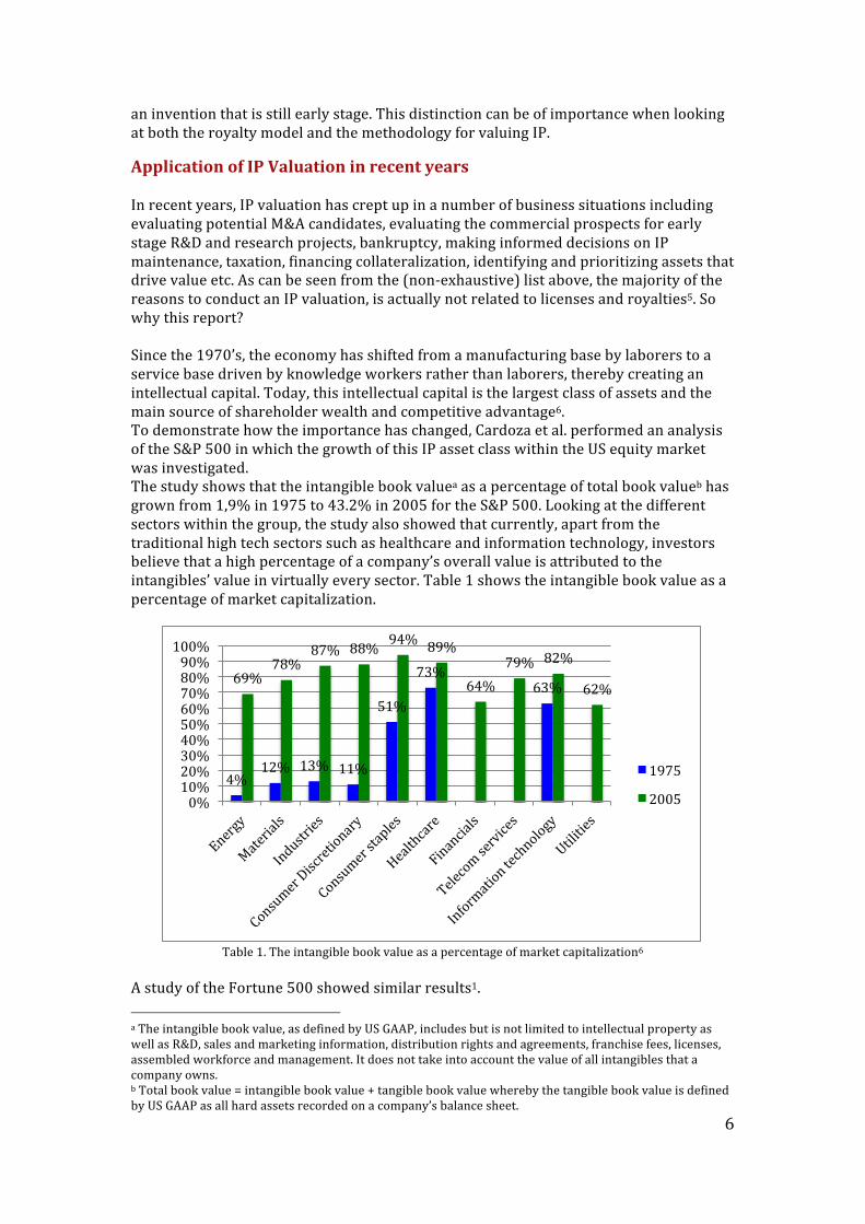
Application of IP Valuation in recent years In recent years, IP valuation has crept up in a number of business situations including evaluating potential M&A candidates, evaluating the commercial prospects for early stage R&D and research projects, bankruptcy, making informed decisions on IP maintenance, taxation, financing collateralization, identifying and prioritizing assets that drive value etc. As can be seen from the (non-‐exhaustive) list above, the majority of the reasons to conduct an IP valuation, is actually not related to licenses and royalties5. So why this report? Since the 1970’s, the economy has shifted from a manufacturing base by laborers to a service base driven by knowledge workers rather than laborers, thereby creating an intellectual capital. Today, this intellectual capital is the largest class of assets and the main source of shareholder wealth and competitive advantage6. To demonstrate how the importance has changed, Cardoza et al. performed an analysis of the S&P 500 in which the growth of this IP asset class within the US equity market was investigated. The study shows that the intangible book valuea as a percentage of total book valueb has grown from 1,9% in 1975 to 43.2% in 2005 for the S&P 500. Looking at the different sectors within the group, the study also showed that currently, apart from the traditional high tech sectors such as healthcare and information technology, investors believe that a high percentage of a company’s overall value is attributed to the intangibles’ value in virtually every sector. Table 1 shows the intangible book value as a percentage of market capitalization.
Table 1. The intangible book value as a percentage of market capitalization6
A study of the Fortune 500 showed similar results1. a The intangible book value, as defined by US GAAP, includes but is not limited to intellectual property as well as R&D, sales and marketing information, distribution rights and agreements, franchise fees, licenses, assembled workforce and management. It does not take into account the value of all intangibles that a company owns. b Total book value = intangible book value + tangible book value whereby the tangible book value is defined by US GAAP as all hard assets recorded on a company’s balance sheet.
4% 12% 13% 11%
51%
73% 63% 69%
78% 87% 88%
94% 89%
64% 79% 82%
62%
0% 10% 20% 30% 40% 50% 60% 70% 80% 90% 100%
1975
2005

7
Another trend that has been observed in the technology-‐based economy, is that a lot of the technology-‐based products are not necessarily invented in the company bringing the product to the market but may have derived from external parties7. This so called “open-‐innovation” often results in partnerships whereby risk and reward is shared. The purest form of this “technology transfer activity” is often seen between academic institutions and commercial partners; a new technology is licensed to a commercial partner who is prepared to invest in the development of the invention and bring it to the market. Often, early stage research (pre-‐R&D) is still required and carried out within the academic institutions. As the technology is developed further and further, the company’s role becomes more prominent and eventually takes over. “Technology Transfer” can also be found amongst commercial partners but in different forms. This can be for a number of reasons: sometimes each party brings different knowledge or experience to the table that is necessary to make a successful product. This often results in joint-‐ventures or strategic alliances. The joint venture between Philips and Sony regarding the CD is such an example. Other forms of technology transfer activities between commercial parties – such as out-‐licensing activities similar to those in academic institutions -‐ may also be the result of a company having developed multiple technologies, preferring to focus on 1 and selling or licensing the other (often competing) technologies to its competitors. By doing so, the company does not bet on 1 technology (which is extremely risky), but rather spreads its risk and therefore also its rewards. The High Definition (HD) technology marketed by Philips and the Blue Ray invention marketed by Sony is such an example. Philips invented both technologies. In all of the above cases, assignment of IP or licensing of IP requires valuation.
Assignment versus Licenses A firm can choose to sell IP or license IP. Again, reasons for this may vary. Sometimes inventions are made in areas that the company is not active in itself. Rather than “throwing it out”, it may choose to sell it to another company. The profit resulting from the sales price is better than nothing. However, if the technology is in an area that the company is currently not active in but is related to its core activities, it may be more sensible to license the technology out. The reason for this is because with an assignment (“sale”), the selling party sells all its rights – both economic and legal ownership is lost. In a license, the licensing party merely sells the economic ownership but retains the legal ownership. This is sometimes more desirable if the firm wishes to retain the right to conduct research in that area somewhere in the future. Formally, there is a research exemption in most national patent law legislation8. However, this exemption is only applicable to non-‐commercial or experimental research. In practice, this is a very grey area; it can be argued that any R&D in any company is always commercial research. After all, companies cannot afford “academic” research. But even academic institutions may enter this grey area more quickly than they realize: a lot of the medical and biotech research in academic institutions is carried out with the intention to be translational – thereby improving healthcare. The intention to improve healthcare has been argued to be a commercial application especially when collaborating with commercial parties whose main interest, besides improving healthcare, is to make profit. Hence, academic institutions (should) prefer to license

8
their technology rather than assign their rights purely to ensure they retain their academic freedom. In summary, open innovation has resulted in more license transactions than ever before.

9
Chapter 2: Royalty and Royalty Models
What is Royalty? Licenses often incorporate a compensation for the right to use the IP. This compensation is expressed in a royalty rate and building up to that, milestones and/or upfront payments. It would be expected that royalties in critical revenue deals (which have significant impact on the revenue and profitability of a company) and key technology deals (which have a significant impact on the company’s asset portfolio) have a higher rate than those in less critical revenue deals or technology deals. Before looking at how royalty rates are determined, it is important to understand that there are a number of different royalty structures or models. Below is a short overview of the six most common structures, in order of descending risk for the licensee. In practice, many licenses will have a mixture of these elements9.
Lump Sum Paid-‐up or lump sum royalties are a pre-‐established single payment based upon the total perceived commercial value of the technology. For the licensee, the payment will have a direct negative impact upon gross margin performance. However, the advantage is that the licensee has the potential to amortize the per-‐license royalty cost over a larger-‐than-‐expected sales volume, thereby effectively reducing the average license cost as the volume of sales increases. The disadvantage of this royalty model is that the negotiations are dominated by the expected total sales performance. As this is difficult to forecast, the licensee often runs the risk of overpaying. Lump sum payments, as the basic royalty structure, are best applicable in mature markets.
Minimum Royalty Similar to lump sum payments, minimum royalties require a guaranteed payment which is due either at the beginning of the technology transaction or with the commencement of a reporting period (e.g. per month, per quarter, per semester or annually). The advantage of a minimum royalty over a lump sum payment is that the licensee can somewhat reduce its risk by spreading the payment over a number of years. However, it still offers little protection against market volatility or price erosion. Both lump sum payments and minimum royalties are less favorable in license transactions where emerging technologies are involved. The reason for this is that especially with emerging technologies, the risks around forecasting the revenue stream are difficult.
“Fixed Per-‐License” Royalty A “fixed per-‐license” royalty is a running per-‐unit payment, which is fixed over time e.g. a 3% royalty rate. The payments of the royalty are usually tied to the licensee’s actual sales of licenses or units of the technology. If there are no sales, there is no royalty payment. Similar to the models described above, a key consideration for the licensee in determining a fixed per-‐license royalty is that is licensee is able to foresee what the total value of the technology is over the technology’s product life cycle and the anticipated price erosion that may occur if the patent expires over the product life cycle (e.g.
10
medicines) or simply because of declining market relevance (software or high-‐tech electronics). “Fixed per-‐license” royalties are appropriate in mature, more static product markets where historic market data is available (e.g. market oligopolies such as the sublicensing of predominant O/S platforms). The biggest disadvantage is that the price erosion over time is difficult to forecast. Again, this model offers no protection for the licensee against the volatility in decreasing margins or declining markets.
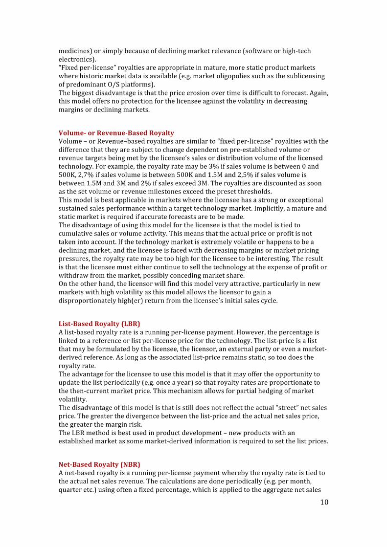
Volume-‐ or Revenue-‐Based Royalty Volume – or Revenue–based royalties are similar to “fixed per-‐license” royalties with the difference that they are subject to change dependent on pre-‐established volume or revenue targets being met by the licensee’s sales or distribution volume of the licensed technology. For example, the royalty rate may be 3% if sales volume is between 0 and 500K, 2,7% if sales volume is between 500K and 1.5M and 2,5% if sales volume is between 1.5M and 3M and 2% if sales exceed 3M. The royalties are discounted as soon as the set volume or revenue milestones exceed the preset thresholds. This model is best applicable in markets where the licensee has a strong or exceptional sustained sales performance within a target technology market. Implicitly, a mature and static market is required if accurate forecasts are to be made. The disadvantage of using this model for the licensee is that the model is tied to cumulative sales or volume activity. This means that the actual price or profit is not taken into account. If the technology market is extremely volatile or happens to be a declining market, and the licensee is faced with decreasing margins or market pricing pressures, the royalty rate may be too high for the licensee to be interesting. The result is that the licensee must either continue to sell the technology at the expense of profit or withdraw from the market, possibly conceding market share. On the other hand, the licensor will find this model very attractive, particularly in new markets with high volatility as this model allows the licensor to gain a disproportionately high(er) return from the licensee’s initial sales cycle.
List-‐Based Royalty (LBR) A list-‐based royalty rate is a running per-‐license payment. However, the percentage is linked to a reference or list per-‐license price for the technology. The list-‐price is a list that may be formulated by the licensee, the licensor, an external party or even a market-‐derived reference. As long as the associated list-‐price remains static, so too does the royalty rate. The advantage for the licensee to use this model is that it may offer the opportunity to update the list periodically (e.g. once a year) so that royalty rates are proportionate to the then-‐current market price. This mechanism allows for partial hedging of market volatility. The disadvantage of this model is that is still does not reflect the actual “street” net sales price. The greater the divergence between the list-‐price and the actual net sales price, the greater the margin risk. The LBR method is best used in product development – new products with an established market as some market-‐derived information is required to set the list prices.
Net-‐Based Royalty (NBR) A net-‐based royalty is a running per-‐license payment whereby the royalty rate is tied to the actual net sales revenue. The calculations are done periodically (e.g. per month, quarter etc.) using often a fixed percentage, which is applied to the aggregate net sales

11
by the licensee over the reporting period. It is similar to the “fixed per-‐license” royalty and the LBR with the difference that the NBR’s variability is wholly dependent on the actual street price performance of the technology. However, revenue-‐based NBR royalty is also possible. NBR is the most attractive royalty model for preserving sustained margins for licensed technologies, especially when engaging in emerging or highly volatile markets. The disadvantage of this model is mostly with the licensor: NBR’s effectively present unlimited upside and downside potential. Under the NBR model, technologies licensed in significantly volatile or declining markets will generate the greatest variance in net revenue. Another disadvantage of this model for the licensor is that the licensee may seek to “bundle” the technology with other technologies the licensee may have. Net-‐based royalties can either be a fixed rate or a revenue-‐ or volume-‐based royalty rate.
Payments Prior to Royalty Royalty payments are received by the licensor when products are actually sold. However, in many license transactions, the technology still needs to be developed. In some sectors, such as biotech or pharmaceuticals, this can take more than 10 years if it happens – a large amount of the technologies licensed out a proof-‐of-‐principle stage will never make it through the clinical trials or market approval. In these situations, financial compensation may be awarded prior to royalty payments through upfront fees, annual fees and milestone payments, which in essence are “in advanced received” royalties. The amounts set for these advanced payments are often taken into account in the royalty rate negotiations.
When Are Royalty Rates Set? It is important to understand that licenses are often, but not always, negotiated at an early stage. The reason for this is that new inventions require protection before any form of public disclosure has been undertaken. Therefore, patent protection is sought at a very early stage, sometimes before proof-‐of-‐principle has been achieved. Because of the costs involved in patenting, most companies know at the outset if they want to develop the technology themselves or shelve the invention to keep competitors outc or, even if they have no interest in developing the technology themselves, are open to out-‐licensing the technology. In the latter case, potential licensees are identified as soon as possible. As can be seen from the above described royalty structures, with the exception of the LBR and NBR methodology, a forward looking view is required whereby future revenues, investments and other costs need to estimated in order to set a royalty rate for the underlying intangible asset.
c Shelving is when a company chooses to file a patent but not exploit simply to keep others out of the market. Another strategy often used is the disclosure of the inventions companies have no interest in. That way, the technology cannot be filed as a patent by a competitor in the future.

12
Chapter 3. Valuation Models Valuation methods that normally are used to value risky business projects, such as decision tree analysis and Black Scholes option pricing, allow for the incorporation of options. The options give management a degree of flexibility to change strategy if circumstance change of time. Developing new products based on patented technology can be regarded as a high-‐risk operation: developments costs are high, patent costs are high and rate of failure is high. In addition, competitive products could also have a significant impact on the revenues even if the product makes it to the market. A degree of flexibility would therefore be desirable. However, the traditional valuation methods for patents tend to be the less complex methods such as cost-‐based, market-‐based, and (simple) income-‐based techniques10. New York: John Wiley & Sons). The main reason for using these methods is their simplicity in usage. The disadvantage is that they are perhaps too simple and many practitioners have recognized this problem. Since the option pricing techniques are found to be too difficult in use, and the traditional methods insufficient, new hybrid models have been developed by practitioners in the hope to overcome the gap. Often these techniques are a mix of or based on one of the models described above. I have selected 4 models that have been developed as alternatives and have described the basis of the models. The models presented below are actually being used in daily practice. The author does not further analyze the accurateness or logic of the models as this goes beyond the purpose of the report. However, it would certainly be an interesting exercise. The most common techniques are discussed briefly with the intention to get a feel for the different perspectives and approaches each of these methods have11.
Traditional Patent Valuation Methods
Cost Approach – Accounting for (Historical) Costs In the cost approach, different definitions of cost can be applied. The three most common are historical costs, (new) reproduction cost and the replacement cost. In the historical cost definition the historic costs are identified perhaps minus depreciation or obsolescence. It is the least appropriate of all methods. It takes no future benefits into account. The reproduction cost is a forward-‐looking perspective and aims to calculate the total cost, at current prices, to develop an exact duplicate of the IP. However, this would imply the company is infringing the patent and this may bring other costs to the project (e.g. court claims)11. The cost approach using a replacement cost definition is also a forward-‐looking perspective on how to create an asset that has the same or similar functionality as the asset in question9,12. However, there is something counter-‐intuitive about this approach. If it is relatively easy to invent around the patent, then it could be argued that the patent has little value to begin with13. The cost measurement in the replacement cost new method consists of 4 elements: direct costs, indirect costs, the IP developers profit and the opportunity cost/entrepreneurial incentive. The first two cost elements are easy to identify and quantify. The third cost element, the IP developer’s cost, is often estimated as a percentage rate of return on the total investment in the material, labor and overhead

13
costs. The entrepreneurial incentive is measured as the loss in profit during the replacement IP development period. For example, if a firm were to take a license to a patent that has been developed into a product ready for sales, it would have an immediate revenue stream (either operating income or licensing income). However, if the firm chooses to develop its own IP, which is, for example, estimated to be 2 years, then the firm “loses” 2 years of profit. This amount is regarded to be the entrepreneurial incentive. It is important to realize that this can only be calculated in the event the patent actually has been developed into a product or there is a very similar product already on the market and you actually can measure what the profits are that one loses out on. However, this is not often the case. The approach, while useful in the situation where there is no other available data – wholly disregards the innovation and uniqueness of the IP. The cost-‐based approach, as mentioned above, has also been criticized due to its inability to account for potential future profits. (LEES).
Market/Transactional Approach – Accounting for Market Conditions The market approach is the most simple to understand: it is the actual price paid for a similar intangible under similar circumstances, also known as the Comparable Uncontrolled Transactional (CUT) method. Some firms may use a related methodology referred to as the Comparable Profit Margin (CPM) method5. Although both are comparative analyses, the basis is different. In the CUT method, comparable sales and licenses of IP are identified whereas in the CPM method the analyst is looking for comparable sources of supply (similar customers, same type of products) but with the difference that the comparable companies have generic trademarks and produce unpatented products. The enhanced economic benefit that the IP provides is the difference between the margin of the guideline companies and the subject company. The incremental profit margin is the implied royalty rate. In the CUT method, there are essentially two steps: 1) the screening and 2) the adjustment. In the screening step, the analyst seeks to obtain information of the comparison attributes (e.g. the IP, the use of IP, the industry, date of sale or license etc.), verify the accurateness of the information and select the relevant units of comparison (e.g. income pricing multiples or dollars per unit). In the adjustment step, the guideline IP is compared to the subject IP and the sale or license price of each guideline transaction is adjusted for any differences between the guideline IP and the subject IP. Subsequently, pricing metrics are selected from the range of pricing metrics derived from the guideline transactions and applied to the subject IP transaction. The market-‐based approach is theoretically feasible for inventions that are regarded as (small) improvements for existing technologies rather than groundbreaking inventions where comparability is limited. Adjusting, too, much may compromise the credibility of the transactional method.
Income approach – Accounting for Future Value The income method is in many ways the most fundamental of the valuation methods; it is based on the ability of the asset to generate future income. The future income is discounted in some models and then reflects the present value of the asset. Cash flows are generally forecasted explicitly throughout the expected economic life of the IP. Beyond the economic life of the asset an estimate of remaining value or terminal value

14
may be appropriate. Although, the income-‐based approach is theoretically valid, the problem here lies in the difficulty of estimating future cash flows. The method requires a degree of subjectivity when assessing all the business and financial dynamics that impact the expected incremental cash flow. However, despite the subjectivities, the income-‐based approach has become most popular among practitioners, mainly due to its ability to carry out what-‐if analyses.
25% Rule of Thumb The 25% Rule has been used for over 40 years but still continues to be used by many in spite of the numerous critiques its had, mostly because of lack of convincing evidence to empirically validate the 25% rule14,15. The Rule suggests that the licensee pay a royalty rate equivalent to 25% of its expected profits for the product that incorporates the IP at issue. It is therefore a method that falls under the income approach. In its pure form, the Rule is as follows. An estimate is made of the licensee’s expected profits for the product that embodies the IP at issue. Those profits are divided by the expected net sales over that same period to arrive at a profit rate. It is important to note that the fully loaded profit should be used and not the gross profit. The gross profits exclude costs related to marketing, R&D and SG&A. By applying the rule to gross profits, the economic benefit gained as a result of the patent would be overstated. The fully loaded profit margin is then multiplied by 25% to arrive at a running royalty rate. The advantage of this method is that it is very simple to understand and apply. The primary disadvantage of this rule is that is does not take into account specific circumstances around the company, industry and factors that will determine the actual value of the patent at issue. It has been argued by many that the 25% rule should be used as a starting point or in addition to another valuation method, merely to perform a sanity-‐check14,15,16.
DCF – Accounting for Time and Uncertainty The two key factors they account for are the time value of money and to some extent the riskiness of the forecast cash flows. These two problems can be solved in two ways: the first method accounts for both factors at the same time (standard DCF) and the second method in which the riskiness of the cash flows is removed to be subsequently discounted at the risk free rate (certainty equivalent cash flow method) The latter method separates the two issues of risk and time and can help avoid problems when the risk adjustment varies over time as it will with patents. One advantage of valuing patents with DCF methods is that since patents have limited lifetimes one is not faced with the problem of estimating residual values for the cash flows beyond the edge of the forecasting horizon. The biggest criticism the traditional DCF has is that it doesn’t allow for any managerial flexibility and that the outcome of the project is not in any way affected by the decisions made by management during the course of the project.
The More Complex Valuation Models High-‐risk projects or high-‐risk new business segments that are explored by a firm can be valued using real option techniques. These methods are all based on models where the conditional events required for the IP to generate income are modeled explicitly. In other words, the models take an income approach. This is often desirable if the project or undertaking requires a significant investment and has an uncertain payoff.

15
From that perspective, patents can be regarded as similar investment projects: often significant amounts of money are required to develop the patent into a product and the investments have a highly uncertain payoff. There are three models to be identified: decision tree analysis, and binomial tree Black & Scholes Option Pricing.
Decision Tree Analysis – Accounting for Flexibility At the core of this method, two steps can be identified: 1) computing the probability that a certain event or variable will occur and 2) the financial implication of that event or variable occurring. The events can have either a positive or negative impact. Depending on the effect of the event, management is given the flexibility to adjust its strategy accordingly. This could save the company unnecessary investments. The down-‐side of this method is that, although simple to use for a limited number of variables, it gets very complex when there are many uncertain factors.
Option Pricing Model: Monte Carlo Simulation– Accounting for Riskiness (continuous time) Option-‐pricing models were originally developed to value financial options but it soon became clear that the models could also be applied to real assets. The underlying assumption of real-‐ option models is that the solution to the problem posed requires a probability-‐approach, not only at present time but at all instances in time up to the maturity of the option (e.g. option to expand a project or option to abandon a project). Therefore, it is a continuous-‐time model. The uncertainties related to the value of the real asset are modeled as a stochastic process. The value of an option problem at a certain point in time, in terms of payoff, is based on the initial choices the company has made and the remaining options that result from those initial choices taking the stochastic processes into account. As in the decision tree analysis, this model allows management to be flexible and change strategy when appropriate17.
Option Pricing Model: Binomial Tree – Accounting for Riskiness (Discrete Time) A more transparent model is the binomial tree approach. The model was originally designed to value options to buy or sell financial instruments, such as stock. A discrete approximation to the underlying stochastic process was developed to make a more (computational) efficient model. The model uses binomial lattices or a probability tree with depicts two possible changes whereby the outcome is the result from moving up (u) or down (d) in value17. An example of this type of binomial lattice is shown in Figure 1, where S is the current market price of the asset. There is a q probability of an upward move and there is a 1-‐q probability that the market price will go down and result in Sd. U is a factor greater than 1, and d is the reciprocal of u. In Node Su, there is a q probability that the price will go up resulting in Suu and a 1-‐q probability that the price will go down resulting in Sud. The latter node can also be reached if the Sd node increases in price.
Su
Suu
Sd
Sud / Sdu S
q
1-‐q

16
Figure 1: Binomial lattice
To find the present value with options with such a lattice, we start from the final time period, depicted on the right hand side of the tree, and work backwards through time. Finding the value from exercise or deferral of the option at each node in each period will eventually lead us to the starting point (time zero), which is on the left hand side of the tree. At nodes where the value has gone up, the optimal decision for a call option (option to buy the stock), for example, would be to exercise, while at nodes where the value has gone down, the optimal decision would be not to exercise. The opposite policies would generally be true for a put option (option to sell the stock).
It is important to accurately assess the level of risk associated with the option exercise decision at each node because it dictates how much future cash flows (option payoffs) should be discounted during the backward induction process. This presents a challenge because the risk level is not constant, but is specific to each node in the lattice.
As mentioned above, the change in value can either go up or down and is dependent on the probability q. To adjust the risk-‐level, the model uses the following approach. It uses probabilities that a risk-‐neutral investor would assign to the outcomes. Thus, in a similar manner as q, p is the risk-‐neutral probability for the outcome Su and 1-‐p is the risk-‐neutral probability for the outcome Sd. Because of the risk-‐neutral nature of the assigned probability, the discount rate used discount the cash flows is the risk-‐free rate.
To calculate p, the model requires the volatility (σ) of the asset per time increment as well as the length of the time increment (t). With this information, u can be calculated (u = eσ√Δt) and d follows from u (d = 1/u). Once u and d have been determined, the probability for an up move at each node in the tree is then p = (1 + rΔt – d)/ (u-‐d), while the corresponding probability of a down move is simply 1-‐p, as mentioned above. However, the process of working through lattices can be cumbersome and non-‐intuitive, especially for more complex applications to real assets, which can involve several simultaneous and compound options. Because of the increased importance of IP in the world (see Table 1, Chapter 1), it is expected that these more sophisticated techniques will become more widely used. However, at this point in time, it is often still regarded as too complex.
Hybrid Models As the above described models have been found to be either too simplistic or too complex, many practitioners have developed hybrid models. As mentioned above, 4 models have been selected that have been developed as alternatives and have described the basis of the models. The models presented below are actually being used in daily practice. The author does not analyze the accurateness or logic of the models as this goes beyond the purpose of the report but merely wishes to demonstrate the need identified by practitioners for better manageable methods for those who are challenged with determining royalty rates.
Sdd
17
Hybrid Model 1 (Institut Curie) The Institut Curie has developed a method based on the 25% rule income rule19. They propose the use of a “simplified provisional profit and loss statement” whereby two phases are identified: 1) pre-‐marketing phase during which there are only expenses and no revenues (R&D costs, patent registration costs, pre-‐production costs etc.) and 2) a marketing phase during which costs are still incurred but where a revenue stream is generated. The moment between the two phases is noted as M0. The costs in phase 1 are estimated each year, subsequently added together and then discounted by a discount factor (typically to be between 8% and 20% and is defined as the return on investment the licensee would have had if it would have invested these resources in its own business). The discounted sum is subsequently amortized in the second phase. In the second phase, costs are split into expenses and investments, which can be amortized as well. The benefit per yearx is calculated as SalesX -‐ Production costsX – Marketing costsX – Residual R&D costsX – Amortized investmentsX consisting of the discounted costs from phase 1 and any other investments from phase 2 that can be amortized. At the beginning of the second phase, costs may be higher than revenues. Therefore, an “Average Provisional Benefit” (APB) is calculated which is the sum of the benefit calculated per year for the projected forecast divided by the number of years. Similarly, the average of sales is calculated (APS). It should be noted that the amounts in phase 2 are not discounted. APB is then expressed as a percentage of APS. The last step in this model is determining the ratio of sharing the APB. The 25% rule is the basis that is used. The licensee and the licensor merely need to agree on the split of the APB e.g. 75/25 or 66/33. This percentage is then multiplied by the ratio APB/APS. For example, if the APB/APS ratio is 25% and the agreement on the split of the APB is 25% for the licensor, the royalty rate is 25% x 25% = 6,25% The main advantage of this model is that it is simple to understand and the assumptions are relatively easy to identify. In addition, the model allows for corrections when introducing milestones and upfront payments. It combines DCF with the standard 25% rule.
Hybrid Model 2 (Syracuse University) The basis assumptions and key variables in this method are that the value of the IP is directly related to the value of the product that incorporates the IP20. More specifically, the value of the IP can be measured as the competitive advantage that it contributes to a product, process or service. The key variables are the NPV of the cash flows of the product utilizing the product and the competitive advantage contribution of the IP to the NPV. This method is aimed at the valuation of patent licenses and involves 5 steps and an optional sixth step. The first step is the identification of the patents that are associated with a product. The product will have certain competition parameters compared to average substitute products. The patents are then linked to the specific competition parameters. For example, a new biosensor product consists of two components: a sensor and a reader. The competition parameters for the sensor are sensitivity and the competitive parameter for the reader is portability. Patent X is associated with the sensitivity parameter and patent Y is associated with portability

18
The second step is the calculating the base competitive advantage contributions of the patents by comparing the associated product to the average substitute product. Subsequently, the contribution of the individual patents to the associated product is calculated. For example, the average substitute biosensor has a sensitivity of 1000 pathogens. The associated product has a sensitivity of 200. The base competitive advantage is (1000-‐200)/1000 = 0.8. Similarly, the base competitive advantage for the reader (portability) could be 0.5. The total base competitive advantage is 0.8 + 0.5 = 1.3. The relative competitive advantage of the sensor patent is 0.8/1.3 = 0.615 and the relative competitive advantage of the reader patent is 0.5/1.3 = 0.385. Thirdly, the NPV of the associated product is calculated and a fraction of the NPV is attributed to the IP assets. The product’s NPV calculation requires information on the current year’s sales, the expected growth rate, expected life of the technology, net profit margin and a discount rate. The forecasted profit margin is discounted to calculate the NPV. Calculating the fraction of the NPV due to the IP assets is complicated. The model identifies 4 indicators: intangible asset percentage (IA%), Operational IP percentage (OIP%), reputational IP asset percentage (RIP%) and technical IP asset percentage (TIP%). Sales, general & administrative (SG&A) costs are used as an indicator for IA. R&D costs are used as an indicator for TIP. Advertising expense (AD) is used as an indicator for RIP and investments in new business processes (BP) is used as an indicator for OIP. In addition, IP asset percentage (IPA%) and tangible asset percentage (TA%) are also calculatedd. To calculate the percentages, the model uses specific formula’s utilizing the various expenses as indicators.e Having calculated the individual indicators, the IP asset value van be derived (TIP% x NPV of associated product). Fourthly, a portion of the associated products IP asset value is attributed to each patent based on the relative competitive advantage contribution of the products NPV calculated under step 2 and 3. This is done by multiplying the relative competitive advantage (step 2) by the IP asset value (step 3). We assume that the IP asset value under step 3 is €94M. For the sensor, the base value for patent X would be € 94M x 61.5% = € 57.81M and the base value for patent Y related to the reader would be € 94M -‐ € 57.81M = € 36.19M (or 38.5% x € 94M). In the fifth step, the values of the patents are adjusted for IP risk. The IP risk is based on three factors: obsolescence of rights, loss of rights and strength of rights. The obsolescence of rights is a measure of the risk that the patent might become functionally obsolete prior to the expiration of the patent. Loss of rights is a measure of risk that the patent may be found invalid. The strength of rights is a measure of risk that the patent might not adequately protect the patent. This leads to the following formula: the adjusted patent value = patent base value (calculated under step 4) x (100% -‐ sum of the IP risk components). If the obsolescence risk in the above example is estimated to be 0%, the risk of loss is estimated to be 20% and the risk of strength is estimated to be 5%, the total adjustment to be made is (100% -‐ (0% + 20% + 5%)) = 75%. The adjusted value is 75% x € 57.81M = € 43.35M.
d TA% is calculated bookvalue / market capitalization value e IA = (SG&A – AD-‐BP)/(SG&A + R&D) x (100% -‐ TA%) IPA = (R&D + AD + BP)/ (SG&A + R&D) x (100% -‐ TA%) TIP = R&D / (R&D + AD + BP) x IPA% RIP = AD / (R&D + AD + BP) x IPA% OIP = BP / (R&D + AD + BP) x IPA%

19
In addition to the above steps, alternative license payments can be calculated from the adjusted present value of the license, the licensor and the licensee investments in the license, the form of the license payments and the licensee and licensor weighted average cost of capital20. The basis of this methodology appears to be a mixture of an income approach (DCF) and a market approach (competitive advantage of the product to existing products, predicted market share, market adjustments, etc.). Without going into detail, it is obvious from the 5-‐step process that it is a complicated method with numerous assumptions and market data, making the credibility of the method highly questionable.
Hybrid Model 3 (VTT Technical Research Centre Finland) Hytonen et al. present a different framework and focuses on the value of the patent protection itself13. Their approach is as follows: they first identify a number of scenarios that may occur. The scenarios are based on the expected arrival of competing technologies and the size and life cycle of target market. They are often based on specific uncertainties. For example, a company may be aware of competing technologies being developed but does not know when they will arrive on the market and what the impact will be for the technology they are currently developing. In addition, a second uncertainty is the rate of adoption of the new technology – either consumers like the product (big market potential) or they stick to what they have (small market potential). These two uncertainties result in 4 scenarios: 1) high differentiation against competing technologies, big market (P1) 2) low differentiation against competing markets, small market (P2) 3) high differentiation against competing technologies, small market (P3) 4) low differentiation against competing technologies, big markets (P4). The second step in their valuation process is the calculation of future cash flows of the product that incorporates the patented technology. Each cash flow is evaluated with yearly estimates for market size, which was assumed to depend on the prevailing market conditions, and for market share, which was assumed to depend on the differentiation value. The differentiation value is the difference in the customer value between the patented solution and the next best alternative. To calculate the cash flows attributable to the patent protection, the total value of the new technology is split into three components: manufacturer margin, manufacturer costs and technology value. For example, the technology value may be 20% of the total value of the product. The technology value subsequently consists of the patented technology in question and other complementary technology required to produce the product. This, too, is expressed as a percentage e.g. the patented technology in question is 15% of the technology value. This is similar to the approach in Hybrid Model 2 discussed above. The amount of cash flows attributable to the patent protection is calculated by multiplying the forecasted sales levels per year by the fraction of technology value of total value and by the fraction of patent value of all IPR value in the solution for each scenario. In summary, in year 1, there are four different forecasted cash flows, one for each scenario. In year 2, there are again four different cash flows, one for each scenario etc. Mapping the annual cash flows per scenario in a graph, the real options are identified: the scenario in which the cash flows become negative, the option to abandon the patent and, thus, the option to abandon the project is taking into account. This is the only real option that the model looks at.

20
In the final step, the present value of the sum of the cash flows of each scenario is calculated e.g., the present value of all the cash flows under scenario 1 are €1.8M. This sum is then multiplied by the probability of each scenario derived from market information or from experts. For example, the probability of a high differentiation value against competing technologies is 0.6 and the probability of a big market is 0.3. Therefore, the probability of a low differentiation value against competing markets is 0.4 (1-‐ 0.6) and the probability of a small market is 0.7 (1-‐0.3). Thus, scenario P1 = 0.18 (0.6 x 0.3), scenario P2 = 0.28 (0.4 x 0.7), scenario P3 = 0.42 (0.6 x 0.7), and scenario P4 = 0.12 (0.3 x 0.4). Looking at scenario 1, the NPV outcome would be €1.8M x 0.18 = €324K. This calculation is performed for the other scenarios as well (up to the point of abandonment if applicable). The computed amounts of each scenario are added together to give the value of the patented technologyf. This can then be expressed as a percentage of the overall sales or profit of the full product, which incorporates the patented technology in question. This model appears to be income-‐based (cash flow forecast) and to a lesser extent market-‐based (estimating market size by looking at near markets, similar products etc.) as well. The main disadvantage of this approach is the subjectivity in determining the future cash flows of all products, services, or processes that use the patent being valued and the amount the patent has actually contributed.
Hybrid Model 4 (Boston College) This is a new royalty method aims to connect the academic approach and the real-‐world investment analysis21. The key principle in this model is that it views royalty as the minimum damages award. It is a simplified cash flow analysis whereby the calculated running royalty has a value equal to the difference between the NPV of the infringing project and the NPV of the infringer’s next best alternative (see also Cost Approach methods). The difference is the traditional cost-‐based replacement/reproduction product approach and the replacement/reproduction product approach used here, is that it looks at the potential benefits the replacement product can give rather than the costs, making the it an income-‐based approach. In general, Financial Indicative Running Royalty Model (FIRRM) determines the running royalty as a function of three parameters of the infringing project: the cost of capital, useful economic life of the technology, and the ratio of the NPV of the alternative to the NPV of the infringing project (which measures the ability of the alternative to “replace” the infringing profits) on the condition that the IRR is greater than the cost of capital. The first step in the model is to calculate the NPV of the infringing project. Therefore the project needs to be split into two periods in which the first period consists of investment costs but no sales and the second period in which there are both costs and revenues. This is similar to the first hybrid model discussed. The NPV is calculated by discounting the cost and cash flows using the discount rate. The NPV of the alternative non-‐infringing project can be calculated as a percentage or ratio of the NPV of the infringing project e.g. the NPV of the non-‐infringing project is 25% of the NPV of the infringing project. Once both NPV’s are known, the difference between NPVinfringing and NPVnon-‐infringing is the maximum lump-‐sum royalty. f N.B. The cash flows are said to be discounted to the present value but no discount factor is mentioned or any guidelines as to how to calculate the discount factor. Also, the numbers in the graph in the article seem to be identical as the ones used in calculating the value based on the probability of each scenario.

21
If the royalty is structured to be paid out periodically, the maximum competitive royalty would be the maximum lump sum x (1+discount rate). The present value of the royalty can subsequently be written as a percentage of revenue or profits, which then gives the running royalty rate. The above approach, like the first model, appears to be income-‐based.

22
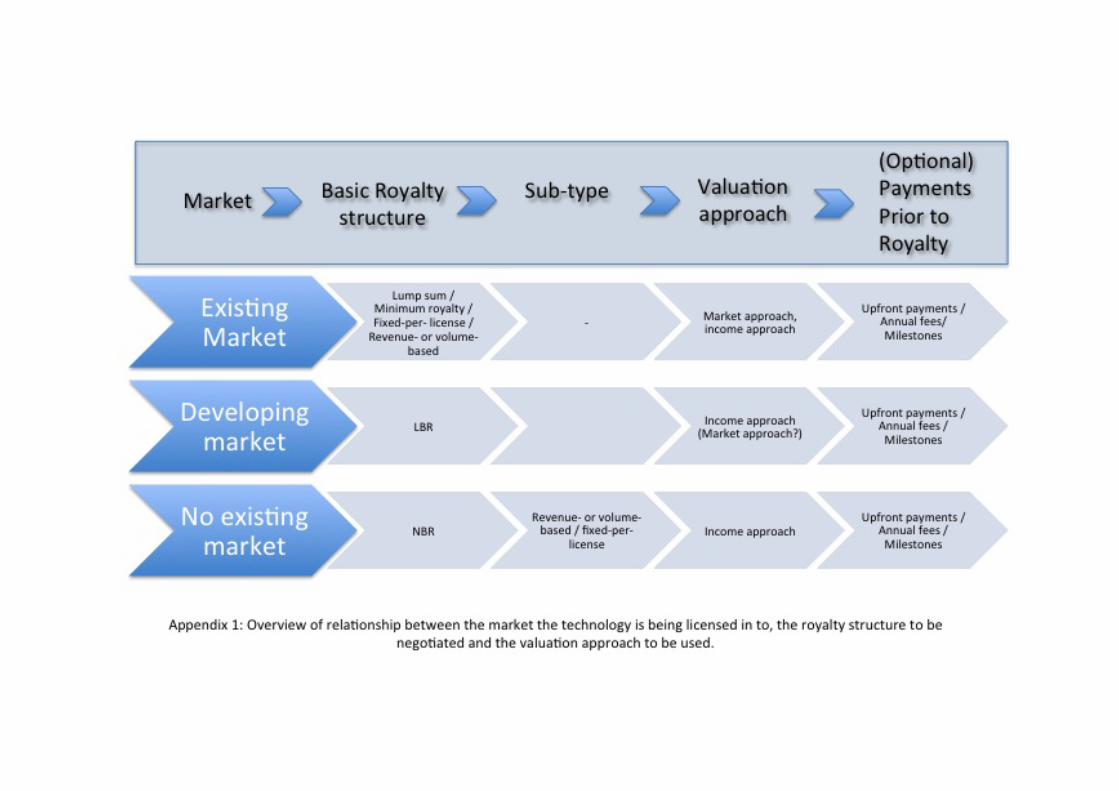
Discussion & Conclusions The two most common methods for valuing IP and determining royalty rates are the market approach and income approach (standard DCF). The CUT and CPM market approach is the easiest to use and is the most popular for many license agreements. DCF analysis is more frequently used by venture capitalists for investment reasons in exchange for shares rather than royalties. As indicated in chapter 4, the hybrid models all seem to incorporate an income-‐based approach. Some have added elements of the market approach to those models as well. The way they use the income and market elements in their models varies significantly. The diversity of the hybrid models seems to have evolved from lack of knowledge of applying real option techniques and the need to have a more advanced model than the traditional methods used to value IP. Some of the more advanced hybrid models, however, appear to be just as complex as the binomial lattices and B&S calculations. Setting aside whether it is possible to combine the various elements the way the hybrid methods do, a vital question appears to be missing in all of the models: can the valuation model be applied to any technology, product or market and how does this relate to the royalty structure chosen? None of the hybrid models discuss any of these elements thereby suggesting they are applicable to any situation. In the author’s view, the approach to using a certain valuation model (income-‐based or market-‐ based) and designing a royalty structure need to be matched to the (future) product and (future) market. Before going back to the hybrid models, it is important to understand how the technology, the market, the royalty structure and the traditional valuation models all interact together. First of all, when evaluating a technology or invention a standard due diligence should be carried out consisting of evaluating the technology, the patentability and the market potential. Looking at the market potential includes the identification of a market and then determining if that market already exists, is developing or non-‐existent. This is important when negotiating a license, as some of the royalty structures are more appropriate or optimal for certain types of markets than others. For example, a “fixed-‐per-‐license” royalty structure is appropriate in mature, static markets where historic data is available whereas a net-‐based royalty is more appropriate in emerging markets or markets with high volatility. Having identified the type of market and its presence or lack thereof and the appropriate royalty structure, the valuation model to determine what the rate should be should match accordingly. For example, a new gene-‐therapy for muscle disorders is a technology in an emerging market. There is no approved gene therapy yet available for any disease so trying to find historical data is futile. A fixed-‐fee per license would therefore not be the most optimal royalty structure for either licensor or licensee. For the licensee, selecting a fixed fee per license royalty structure for a technology that has no comparable historic data poses the risk of overpaying and there is no information with regard to price erosion. For the licensor, this royalty structure would have disadvantages as well. The danger for the licensor is that the technology is “downgraded” and a too low royalty percentage is negotiated simply because data for a different market is used. Therefore a net-‐based royalty is a good alternative for both parties. Having established there is no current market for gene-‐therapy and therefore no historic data and having selected the appropriate royalty structure, the valuation

23
approach that would naturally follow is the income approach. Yet, in practice, many practitioners still turn to a CUT or CPM market approach in this final step. Often licenses will contain different royalty elements particularly in projects where development time is high. Besides the royalty at the end of the line, upfront payments, annual fees and milestones are built into the license. In essence, these are equivalent to lump sum payments and minimum annual royalties. Appendix 1 shows a simple overview of the most optimal royalty structures and the valuation models used to determine the rate. The table is merely an attempt to logically classify the structures so that the outcome is optimal and fair for both parties when properly applied. Turning to the hybrid models, the first model is a form of DCF combined with the 25% rule. As an income-‐based approach, according to Appendix 1, it would work well for determining a royalty rate in any type of market. Looking at the model specifically, it appears to works for any technology, whatever stage of development in any type of market. The model may need to be modified slightly (e.g. discount the second phase and perhaps guidelines to discount rate justification are required) but overall seems to offer a workable and manageable model halfway between the traditional methods and the more complex methods. The model even allows for the optional payments of milestones and upfront payments to be taken into account when determining the royalty rate. The second and third model both are a combination of a market approach and an income approach. Looking at Appendix 1, it would automatically follow that these models would be best applicable in license deals for technologies in an existing market but less appropriate in developing and non-‐existing markets. A big disadvantage of these two models is that it does not take into account the when the license deals are signed off or how far the product development is. If the license is signed when significant R&D is still required, it is very difficult to predict what the technological value of the product is and how much the patented technology is expected to contribute to the technological value, especially if another 10-‐15 years of development work is required. In addition, both models calculate the competitive advantage of the associated product and the average substitute product. It is highly questionable if a competitive advantage percentage can be calculated based on hypothetical competing product that is also to be developed in 10-‐15 years time. The models would therefore really only be applicable to existing products in a mature market. The fourth model, FIRMM, is income-‐based as well. However, although it looks at forecasted cash flows, the method makes use of a comparison between the “infringing” project and the “non-‐infringing” project therefore implying an alternative product is available. There are situations where this is not the case. For example, in the healthcare sector, some diseases do not have a therapy at this point in time. The next best alternative is symptomatic care, which often consists of administering more than 1 product to the patient (e.g. mucolipidoses). In some cases symptomatic care is not even available (e.g. Huntington’s disease). This could complicate the use of this model in certain situations. The model would not be ideal for valuing technologies in emerging markets.
24
Alternative approaches Based on the information given above, it is very difficult to come up with a model “that fits all” although the first hybrid model discussed seems to come very close. Further analysis of the model is required to confirm this. Other alternatives that may tackle the problem of the many uncertainties without using complicating real-‐option techniques is to simply agree that royalty rates need to be revisited on a regular basis. Whether that basis is annually or every 5 years could be dependent on the product, the R&D still required, the development of the market etc. Revisiting commercial terms is not unheard of; in long-‐running successful license deals it regularly happens that the terms are amended to current standards. This is, in fact, the underlying principle of the LBR structure and there is no apparent reason why this approach cannot be used in other royalty structures. By revisiting the license terms after a period of time, the parties can either make use of newly available market data that wasn’t available at the time of the contract negotiation or parties can choose to revisit the income-‐based calculation and correcting for forecast and/or discount factor appropriately and if necessary. This “model” would be applicable in license transactions between industrial parties but also in transactions involving industrial parties and academic parties. Looking at academic institutions involved in industrial research, a more pragmatic way of dealing with royalties may be to move to a standard paid-‐up license (lump sum royalty structure). However, rather than calculating the royalty rate through complicated models or models that insufficiently reflect / cover the uncertainties, a simple standard percentage on top of the research value of the project may be applied. For example, a large pharmaceutical company may be engaged in research collaboration with an academic institution. The value of the research project (full-‐cost) is €1.2M. At the start of the project, there is no IP developed yet. By incorporating 30% of the €1.2M into the deal as a paid-‐up license, the academic institution would have an instant one-‐off royalty stream of 400K. If IP is developed in the course of the project, the company is free to use it and no further royalty payments are required in the future. If no IP is developed during the course of the project, then the 400K is a sunk cost for the company. The risk is with the industrial party. For the academic institution, this may seem like a small amount of royalty-‐stream especially if the invention has a lot of potential. However, in practice many of the licenses that are signed off never generate any income because they don’t make it to the market. The reason for this can vary: a technical problem that cannot be overcome, no financial means, management changes the focus of the company, (in biotech and pharmaceuticals) no market approval is given etc. Looking at the statistics, 95% of the patents filed are never developed into a product therefore only 5% earn money22,23,24. The above would probably not be acceptable in projects amongst industrial parties unless the paid-‐up license sum is significantly higher. The reason for this is that in general companies are profit minded whereas an academic institution does not have a profit-‐making motive. That does not mean that academic institutions should not be compensated – they should be compensated for their contribution to the invention. However, contributing to societal benefits is more important and is the reason why academic institutions may be more open to the above approach.
In summary There is no right or wrong when determining a royalty structure or rate and the results are always the outcome of negotiations. The above structure the author has developed is

25
merely to help select the most optimal royalty structure at the start of the negotiations. Other structures are not necessarily wrong but may pose unnecessary risk for one or both contracting parties. Of the models looked at, it seems that the income approach is more reliable than a market approach or a hybrid model incorporating both. The hybrid model combining two different income approaches (DCF and 25% rule) appears to offer a workable, manageable alternative to practitioners who wish to use a more advanced model than the traditional methods.
26
References 1. Chaplinsky, Susan J. and Payne, Graham, Methods of Intellectual Property Valuation. Darden Case No. UVA-‐F-‐1401. Available at SSRN: http://ssrn.com/abstract=909734 2. WIPO Intellectual Property Handbook: Policy, Law and Use; Retrieved 12 May 2012 from the World Wide Web: http://www.wipo.int 3. Charles Anthon, A Classical Dictionary: Containing An Account Of The Principal Proper Names Mentioned in Ancient Authors, And Intended To Elucidate All The Important Points Connected With The Geography, History, Biography, Mythology, And Fine Arts Of The Greeks And Romans Together With An Account Of Coins, Weights, And Measures, With Tabular Values Of The Same, Harper & Bros, 1841, p. 1273.) 4. Agentschap.nl (2011) Supplementary Protection Certificates, retrieved on 12 May 2012 from the World Wide Web: http://www.agentschapnl.nl/en/onderwerp/supplementary-‐protection-‐certificates 5. Reilly R.F., Intellectual Property Valuation Approaches and Methods, (2011) Les Nouvelles, Vol. XLVI, no. 3, pg. 198-‐209 6. Cardoza K., Basara J. Cooper L., Conroy R., The Power of Intangible Assets: An Analysis of the S&P 500, (2006) Les Nouvelles, Vol. XLI, No. 1, pg. 3 -‐ 7). 7. Chesbrough, H. (2003) Open Innovation: The New Imperative for Creating and Profiting from Technology. Harvard Business School Press 8. Asworth N. (2008), The Research Exception: A Consultation. Retrieved on 17 August 2012 from the World Wide Web: http://www.ipo.gov.uk/consult-‐patresearch.pdf 9. Leal A.G., Applied Royalties in the High-‐Tech Industry, (2011) Les Nouvelles, Vol. XLVI, No. 1, pg. 60-‐68. 10. Smith G.V., Parr R.L., (2000) Valuation of Intellectual Property and Intangibles. New York: John Wiley & Sons 11. Pitkethly R., The Valuation of Patents: A review of patent valuation methods with consideration of option based methods and the potential for further research, Judge Institute, Working Paper WP 21/97, Cambridge. Retrieved on 16 June 2012 from the World Wide Web: http://users.ox.ac.uk 12. Flignor and Orozco (June 2006), Intangible Asset & Intellectual Property Valuation: A Multidisciplinary Approach, Retrieved 12 May 2012 from the World Wide Web: IPThought.com 13. Hytonen H., Jarimo T. (2007), A Scenario Approach to Patent Valuation. Retrieved on 18 May from World Wide Web: http://www3.vtt.fi/liitetiedostot/muut/patentvaluation.pdf 14. Goldscheider R., Jarosz J., Mulhern C., Use of the 25 Per Cent Rule in Valuing IP, Les Nouvelles, Vol. XXXVII, no. 4, pg. 123-‐133.

27
15. Lu J., The 25% Rule still Rules, Les Nouvelles, Vol. XLVI, No. 1., pg. 14–18. 16. Jenai S. (2005), What is a Reasonable Royalty Rate. Retrieved on 15 August 2012 from the World Wide Web: http://www.patentbaristas.com/archives/2005/11/17/whats-‐a-‐reasonable-‐royalty-‐rate/ 17. Brandao et al. Using Binomial Decision Trees to Solve Real-‐Option Valuation Problems; Decision Analysis (2005) 2(2), pp. 69–88, INFORMS. Retrieved on 14 August 2012 from the World Wide Web: http://da.journal.informs.org/content/2/2/69 18. Kodukula P, Papudesu C. (2006), Project Valuation using real options – a practitioner’s guide, , J. Ross Publishing. 19. Salauze D., A Simple Method For Calculating A “Fair” Royalty Rate, 20. Hagelin, Ted, Competitive Advantage Valuation of Intellectual Property Assets: A New Tool for IP Managers. IDEA: The Journal of Law and Technology, Vol. 44, p. 79, 2003. Available at SSRN: http://ssrn.com/abstract=777746 21. Epstein R., Marcus A.J., Economic Analysis of the Reasonable Royalty: Simplification and Extension of the Georgia-‐Pacific Factors. Retrieved on 15 August 2012 from the World Wide Web: http://royepstein.com/epstein-‐marcus_jptos.pdf 22. Sougata Mukherjee (June 8, 1998), South Florida Business Journal. Retrieved on 16 August 2012 from the World Wide Web: http://www.inventionstatistics.com/Innovation_Risk_Taking_Inventors.html 23. Kuczmarski T., Fortune, 12-‐2-‐91 pp. 56. Retrieved on 16 August 2012 from the World Wide Web: http://www.inventionstatistics.com/Innovation_Risk_Taking_Inventors.html 24. Astebro T. (1998), “Basic statistics on the success rate and profits for independent inventors”, Entrepreneurship: Theory and Practice. Retrieved on 16 August 2012 from the World Wide Web: http://www.inventionstatistics.com/Innovation_Risk_Taking_Inventors.html 25. Choi W., Weinstein R. (2001) Analytical solution to Reasonable Royalty Rate Calculations, 41 J.L. & Tech. 49 26. Culbertson J., Weinstein R., Product Substitutes and the Calculation of Patent Damages, Journal of the Patent and Trademark Office Society 70 (1988): 705-‐788. 27. Porter M, Mills R. Weinstein R., Industry norms and Reasonable Royalty Rate Determination, Les Nouvelles, Vol. XLIII, No. 3. pg 47-‐64. 28. Rostoker M.D., PTC Research Report: A Survey of Corporate Licensing, 24 IDEA 59 1983-‐1984 29. Hausman J.A., Leonard G.K., Sidak J.G., Patent Damages and Real Options: How Judicial Characterization of Non-‐Infringing Alternatives Reduce Incentives to Innovate, Berkeley Tech. Law J. Vol. 22:825-‐853.

28
30. Martin G.R., Fernandez P.L., Real Options in Biotechnological Firms Valuation: An Empirical Analysis of European Firms, J. Technol. Manag. Innov. (2006), Vol.1, No. 2. 31. DeSouza G., Royalty Methods for Intellectual Property, Business Economics, (1997); 32,2 pg. 46 ABI/INFORM Global 32. Ziedonis A.A., Real Options in Technology Licensing, Management Science, (2007), Vol. 53, No. 10, pg. 1618-‐1633.

29
APPENDIX