Embed Size (px)
Citation preview
Fast 3D frequency-domain full-waveform inversion witha parallel block low-rank multifrontal direct solverApplication to OBC data from the North Sea
Patrick Amestoy1 Romain Brossier2 Alfredo Buttari3 Jean-Yves LrsquoExcellent4 Theo Mary5Ludovic Meacutetivier6 Alain Miniussi7 and Stephane Operto7
ABSTRACT
Wide-azimuth long-offset ocean bottom cable (OBC)oceanbottom node surveys provide a suitable framework to performcomputationally efficient frequency-domain full-waveform inver-sion (FWI) with a few discrete frequencies Frequency-domainseismic modeling is performed efficiently with moderate compu-tational resources for a large number of sources with a sparse mul-tifrontal direct solver (Gauss-elimination techniques for sparsematrices) Approximate solutions of the time-harmonic waveequation are computed using a block low-rank (BLR) approxima-tion leading to a significant reduction in the operation count andin the volume of communication during the lower upper (LU)factorization as well as offering great potential for reduction inthe memory demand Moreover the sparsity of the seismic sourcevectors is exploited to speed up the forward elimination step dur-ing the computation of the monochromatic wavefields The rel-evance and the computational efficiency of the frequency-domain
FWI performed in the viscoacoustic vertical transverse isotropic(VTI) approximation was tested with a real 3D OBC case studyfrom the North Sea The FWI subsurface models indicate a dra-matic resolution improvement relative to the initial model built byreflection traveltime tomography The amplitude errors intro-duced in the modeled wavefields by the BLR approximation fordifferent low-rank thresholds have a negligible footprint in theFWI results With respect to a standard multifrontal sparse directfactorization and without compromise of the accuracy of the im-aging the BLR approximation can bring a reduction of the LUfactor size by a factor of up to three This reduction is not yetexploited to reduce the effective memory usage (ongoing work)The flop reduction can be larger than a factor of 10 and can bringa factor of time reduction of around three Moreover this reduc-tion factor tends to increase with frequency namely with the ma-trix size Frequency-domain viscoacoustic VTI FWI can beviewed as an efficient tool to build an initial model for elasticFWI of 4C OBC data
INTRODUCTION
Full-waveform inversion (FWI) (Tarantola 1984) is now rou-tinely used in the oil industry as part of the seismic imaging work-flow at least in soft geologic environments such as the North Seathat make the acoustic parameterization of the subsurface accept-
able (for a discussion on this latter issue see Barnes and Charara2009 Plessix and Perez Solano 2015) However it remains a com-putational challenge due to the huge number of full-waveform seis-mic modelings to be performed over the iterations of the FWIoptimization Seismic modeling and FWI can be performed either
Manuscript received by the Editor 25 January 2016 revised manuscript received 10 May 2016 published online 07 September 20161Universiteacute Toulouse III Paul Sabatier Institut National Polytechnique de Toulouse (INPT)-Institut de Recherche en Informatique de Toulouse (IRIT) Tou-
louse France E-mail amestoyenseeihtfr2Universiteacute Grenoble Alpes Institut des Sciences de la Terre (ISTerre) Grenoble France E-mail romainbrossieruniv-grenoble-alpesfr3Universiteacute Toulouse III Paul Sabatier Centre National de la Recherche Scientifique (CNRS)-IRIT Toulouse France E-mail abuttarienseeihtfr4Universiteacute de Lyon Institut national de recherche en informatique et en automatique (INRIA)-Laboratoire de lInformatique du Paralleacutelisme (LIP) LIP Ecole
Normale Supeacuterieure (ENS) Lyon INRIA Lyon France E-mail jean-yveslexcellentens-lyonfr5Universiteacute de Toulouse III Paul Sabatier-IRIT Toulouse France E-mail theomaryenseeihtfr6Universiteacute Grenoble Alpes ISTerreLaboratoire Jean Kuntzmann (LJK) CNRS Grenoble France E-mail ludovicmetivieruniv-grenoble-alpesfrfr7Universiteacute Nice-Sophia Antipolis Geoazur-CNRS CNRS Institut de recherche pour le deacuteveloppement (IRD) Observatoire de la Cocircte drsquoAzur Valbonne
France E-mail alainminiussiocaeu opertogeoazurunicefrcopy 2016 Society of Exploration Geophysicists All rights reserved
R363
GEOPHYSICS VOL 81 NO 6 (NOVEMBER-DECEMBER 2016) P R363ndashR383 13 FIGS 6 TABLES101190GEO2016-00521
Dow
nloa
ded
091
216
to 8
820
975
82
Red
istr
ibut
ion
subj
ect t
o SE
G li
cens
e or
cop
yrig
ht s
ee T
erm
s of
Use
at h
ttp
libra
rys
ego
rg
in the time domain or in the frequency domain (eg Plessix 2007Vigh and Starr 2008b Virieux and Operto 2009) Hybrid approachesare also possible where seismic modeling and inversion are per-formed in the time and frequency domain respectively (Sirgue et al2008) In these hybrid approaches the monochromatic wavefields re-quired to perform the inversion in the frequency domain are built onthe fly in the loop over time steps by discrete Fourier transform duringtime-domain modeling (Nihei and Li 2007) Today most FWI codesare fully implemented in the time domain because the good scalabilityand the moderate memory demand of the initial-condition evolutionproblem underlying the forward problem allow one to tackle a widerange of applications in terms of target dimension survey design andwave physics However the time-domain formulation also requiressignificant computational resources to be efficient when thousandsor tens of thousands of (reciprocal) seismic sources are processed inparallelA common parallel strategy consists of distributing these seismic
sources over processors This embarrassing parallel strategy can becombined with shared-memory parallelism andor domain decompo-sition of the computational mesh if enough computational resourcesare available Strategies based on source subsampling (Warner et al2013) or source blending with random or deterministic (ie plane-wave decomposition) encoding (Vigh and Starr 2008a Krebs et al2009) are commonly used to reduce the number of seismic modelingsper FWI iteration However these strategies which reduce the datafold or add random noise in the FWI gradient at each iteration requireincreasing the number of iterations to reach a sufficient signal-to-noiseratio in the subsurface models Considering a computational meshwith n3 degrees of freedom an acquisition with n2 seismic sourcesand assuming that the number of time steps scales to n the time com-plexity of time-domain modeling scales to Oethn6THORN (Plessix 2007)Alternatively seismic modeling and FWI can be performed in the
frequency domain (eg Pratt 1999 Virieux and Operto 2009) Afew applications of 3D frequency-domain FWI on synthetic or realdata are presented in Ben Hadj Ali et al (2008) Plessix (2009) Pet-rov and Newman (2014) Operto et al (2015) Solving the time-har-monic wave equation is a stationary boundary-value problem whichrequires solving a large and sparse complex-valued system of linearequations with multiple right-hand sides per frequency (eg Marfurt1984) The sparse right-hand sides of these systems are the seismicsources the solutions are monochromatic wavefields and the coef-ficients of the so-called impedance matrix depend on the frequencyand the subsurface properties we want to image This linear systemcan be solved either with sparse direct methods namely Gauss-elimi-nation techniques (eg Operto et al 2007) iterative solvers (egRiyanti et al 2006 Plessix 2007 Petrov and Newman 2012 Liet al 2015) or a combination of both in the framework of domaindecomposition methods (eg Sourbier et al 2011)One pitfall of iterative methods is the design of an efficient pre-
conditioner considering that the wave-equation operator is indefiniteMore precisely the iterative approach is competitive with the time-domain approach in terms of operation count as long as the number ofiterations can be made independent of the frequency ie the problemsize (Plessix 2007) It seems that this objective has not yet been fullyachieved although using a damped wave equation as a preconditioneror as such for early arrival modeling decreases the iteration countefficiently (Erlangga and Nabben 2008 Petrov and Newman2012) Processing a large number of right sides leads us more nat-urally toward direct methods because the computation of the solu-
tions by forwardbackward substitutions is quite efficient once alower upper (LU) factorization of the impedance matrix has been per-formed The pitfalls of the direct methods are the memory demandand the limited scalability of the LU factorization that result from thefill-in of the impedance matrix generated during the LU factorizationFill-reducing matrix orderings based on nested dissections are com-monly used to reduce the memory complexity by one order of mag-nitude that is Oethn4THORN instead of Oethn5THORN (George and Liu 1981) Thetime complexity of the substitution step for n2 right-hand sides scalesto Oethn6THORN accordingly and it is the same as the complexity of time-domain modeling The time complexity of one LU factorization (forsparse matrices as those considered in this study) also scales toOethn6THORN The conclusions that can be drawn about the relevancy ofthe direct solver-based approach from this complexity analysis aretwofold the identity between the time complexity of the LU factori-zation and the solution step for n2 right-hand sides requires the num-ber of right-hand sides to scale to n2 Moreover the identity betweenthe time complexity of one LU factorization and time-domain mod-eling for n2 right-hand sides requires us to limit the inversion to a fewdiscrete frequencies Both requirements are fulfilled by wide-azimuthlong-offset acquisitions implemented with stationary-receiver geom-etries (ocean bottom cable [OBC] or ocean bottom node [OBN])On the one hand stationary-receiver geometries involve a large num-
ber of sources and associated receivers in the computational domainfrom which the LU factorization is performed On the other hand thewide-azimuth long-offset coverage provided by these geometries gen-erates a strong redundancy in the wavenumber sampling of the subsur-face target This multifold wavenumber coverage results from theredundant contribution of finely sampled (temporal) frequencies anda broad range of finely sampled scattering angles provided by densepoint-source acquisitions (Pratt and Worthington 1990) The strategyconsisting of coarsening the frequency sampling in the data space toremove the redundancy of the wavenumber sampling in the modelspace has been referred to as efficient FWI by Sirgue and Pratt (2004)The focus of this study is to present an up-to-date status of the
computational efficiency of 3D frequency-domain FWI based onsparse direct solvers with a real OBC data case study from the NorthSea We have presented a first application of 3D frequency-domainFWI on the North Sea OBC data set in Operto et al (2015) which isfocused on a detailed quality control of the FWI results based onseismic modeling and source wavelet estimation Here we show thebenefits resulting from recent advances in the development of a mas-sively parallel sparse direct solver for FWI applications In this studywe solve the linear system resulting from the discretization of thetime-harmonic wave equation with the MUMPS multifrontal mas-sively parallel solver (Amestoy et al 2001 2006) that performsthe LU factorization with a multifrontal method (Duff and Reid 1983)Compared with the results shown in Operto et al (2015) ob-
tained with the public release 501 of MUMPS (MUMPS team2015) two recent developments in this solver which will be madeavailable in the next major release provide further reduction of thecomputational cost First we speedup the forward substitution stepby exploiting the sparsity of the right-hand sides namely the seis-mic source vectors by extending the algorithmic work done forcomputing selected entries of the inverse of a matrix (Amestoy et al2015d) Second we reduce the operation count of the LU factori-zation by exploiting the existence of blockwise low-rank approxim-ants of the elliptic partial differential operators embedded in thetime-harmonic wave equation (Amestoy et al 2015a) The gov-
R364 Amestoy et al
Dow
nloa
ded
091
216
to 8
820
975
82
Red
istr
ibut
ion
subj
ect t
o SE
G li
cens
e or
cop
yrig
ht s
ee T
erm
s of
Use
at h
ttp
libra
rys
ego
rg
erning idea consists of recasting the so-called frontal matrices of theelimination tree in a block representation and compress blocks thathave low-rank properties the effectiveness and accuracy of this com-pression is controlled by a prescribed threshold In the remainder ofthis study we will refer to this approach as the block low-rank (BLR)format-based approximation This BLR format is an alternative toother low-rank formats such as the hierarchically semiseparable(HSS) format that has been proposed for seismic modeling by Wanget al (2011 2012a 2012b) Even though the theoretical complexityof the HSS format is better than that of the BLR format the simplicityand flexibility of the BLR format makes it easy to use in the contextof a general purpose algebraic multifrontal solver Recent work hasanalyzed the theoretical bounds on the complexity of the BLR format(Amestoy et al 2016b) In this study we compare these theoreticalresults with numerical experiments carried out with a 3D FWI appli-cation and we illustrate the potential of the proposed format in reduc-ing the complexity of the multifrontal solverThis paper is organized as follows The first section reviews the
main ingredients of the forward-modeling engine interfaced withthe frequency-domain FWI code We first briefly review the fi-nite-difference stencil with which the time-harmonic wave equationis discretized This stencil must satisfy some specifications so thatthe fill-in of the impedance matrix is minimized during the LU fac-torization The reader is referred to Operto et al (2014) for a moredetailed description of this finite-difference stencil Then we reviewthe basic principles of the multifrontal method its BLR approxima-tion and the strategy implemented to exploit the sparsity of thesource vectors The reader is referred to Amestoy et al (2015a)for a more detailed description of the BLR multifrontal methodThe second section presents the application on the OBC data fromthe North SeaWe first show the nature of the errors introduced by theBLR approximation in the monochromatic wavefields and quantifythe backward errors for different frequencies For a given BLRthreshold the ratio between the backward errors obtained with theBLR and the full-rank (FR) solvers decreases with frequency Thissuggests that a more aggressive threshold can be used as the fre-quency increases hence leading to more efficient compression asthe problem size grows Then we show that the modeling errors havea negligible impact in the FWI results The cost of the FWI in termsof memory and time confirms that the computational saving providedby the BLR solver relative to the FR solver increases with frequency(namely matrix size)We concludewith a strong and weak scalabilityanalysis of the FR and BLR solvers for the subsurface models andfrequencies considered in this case studyThe limited computational resources that have been used to perform
this case study and the limited computational time required to performthe FWI in the 35ndash10 Hz frequency band using all the sources andreceivers of the survey at each FWI iteration highlights the computa-tional efficiency of our frequency-domain approach to process station-ary recording surveys in the viscoacoustic vertical transverse isotropic(VTI) approximation
METHODS
Frequency-domain modeling with block low-rankmultifrontal solvers
Finite-difference stencils for frequency-domain seismic modeling
Frequency-domain seismic modeling with direct solvers definessome stringent specifications whose objective is to minimize the
computational burden of the LU factorization The first specifica-tion aims to minimize the dependencies in the adjacency graph ofthe matrix and hence the fill-in of the impedance matrix during theLU factorization The second one aims to obtain accurate solutionsfor a coarse discretization that is matched to the spatial resolution ofthe FWI (ie four grid points per wavelengths according to a theo-retical resolution of half a wavelength) The first specification canbe fulfilled by minimizing the numerical bandwidth and optimizingthe sparsity of the impedance matrix using finite-difference stencilswith compact spatial support This precludes using conventionalhigh-order accurate stencils Instead accurate stencils are designedby linearly combining different second-order accurate stencils thatare built by discretizing the differential operators on different coor-dinate systems with a spreading of the mass term over the coeffi-cients of the stencil (Jo et al 1996 Stekl and Pratt 1998 Min et al2000 Hustedt et al 2004 Gosselin-Cliche and Giroux 2014)Such stencils are generally designed for the second-order acous-ticelastic wave equations by opposition to first-order velocity-stress equations as the second-order formulation involves fewerwavefield components hence limiting the dimension of the imped-ance matrix accordingly For the 3D viscoacoustic wave equationthe resulting finite-difference stencil has 27 nonzero coefficientsdistributed over two grid intervals and provides accurate solutionfor arbitrary coarse grids provided that optimal coefficients are esti-mated by fitting the discrete dispersion equation in homogeneous me-dia (Operto et al 2007 Brossier et al 2010) The viscoacoustic 27-point stencil was recently extended to account for VTI anisotropywithout generating significant computational overhead (Operto et al2014)The viscoacoustic VTI 27-point stencil results from the discreti-
zation of the following equations
Ahph frac14 s 0 (1)
pv frac14 Avph thorn s 0 0 (2)
p frac14 1
3eth2ph thorn pvTHORN (3)
where ph pv and p are the so-called horizontal pressure verticalpressure and (physical) pressure wavefields respectively The op-erators Ah and Av are given by
Ah frac14 ω2
ω2
κ0thorn eth1thorn 2ϵTHORNethX thorn YTHORN thorn ffiffiffiffiffiffiffiffiffiffiffiffiffi
1thorn 2δp
Z1ffiffiffiffiffiffiffiffiffiffiffiffiffi
1thorn 2δp
thorn 2ffiffiffiffiffiffiffiffiffiffiffiffiffi1thorn 2δ
pZκ0ethϵ minus δTHORNffiffiffiffiffiffiffiffiffiffiffiffiffi1thorn 2δ
p ethX thorn YTHORN
Av frac141ffiffiffiffiffiffiffiffiffiffiffiffiffi
1thorn 2δp thorn 2ethϵ minus δTHORNκ0
ω2ffiffiffiffiffiffiffiffiffiffiffiffiffi1thorn 2δ
p ethX thorn YTHORN (4)
where κ0 frac14 ρV20 ρ is the density V0 is the vertical wavespeed ω is
the angular frequency and δ and ϵ are the Thomsenrsquos parametersDifferential operators X Y and Z are given by part ~xbpart ~x part~ybpart~y andpart~zbpart~z respectively where b frac14 1∕ρ is the buoyancy and eth~x ~y ~zTHORNdefine a complex-valued coordinate system in which perfectlymatched layers absorbing boundary condition are implemented(Operto et al 2007) The right side vectors s 0 and s 0 0 have the fol-lowing expression
3D FD FWI with BLR direct solver R365
Dow
nloa
ded
091
216
to 8
820
975
82
Red
istr
ibut
ion
subj
ect t
o SE
G li
cens
e or
cop
yrig
ht s
ee T
erm
s of
Use
at h
ttp
libra
rys
ego
rg
s 0ethxωTHORN frac14 ω4sethωTHORN shethxTHORNκ0ethxTHORN
~δethx minus xsTHORN
minus ω2sethωTHORNffiffiffiffiffiffiffiffiffiffiffiffiffiffiffiffiffiffiffi1thorn 2δethxTHORN
pZ
timessvethxTHORN minus
1ffiffiffiffiffiffiffiffiffiffiffiffiffiffiffiffiffiffiffi1thorn 2δethxTHORNp shethxTHORN
~δethx minus xsTHORN (5)
s 0 0ethxωTHORN frac14svethxTHORN minus
1ffiffiffiffiffiffiffiffiffiffiffiffiffiffiffiffiffiffiffi1thorn 2δethxTHORNp shethxTHORN
~δethx minus xsTHORN (6)
where ~δ denotes the Dirac delta function xs denotes the source po-sition sethωTHORN is the source excitation term and sh and sv are the twoquantities that depend on the Thomsenrsquos parametersThe expression of the operator Ah shows that the VTI wave equa-
tion has been decomposed as a sum of an elliptically anisotropicwave equation (term between brackets) plus an anelliptic correctingterm involving the factor ethϵ minus δTHORN The elliptic part can be easily dis-cretized by plugging the Thomsenrsquos parameters δ and ϵ in the ap-propriate coefficients of the isotropic 27-point stencil whereas theanelliptic correcting term is discretized with conventional second-order accurate stencil to preserve the compactness of the overallstencilThe direct solver is used to solve the linear system involving the
matrix Ah (equation 1) In a second step the vertical pressure pv isexplicitly inferred from the expression of ph equation 2 beforeforming the physical pressure wavefield p by linear combinationof ph and pv (equation 3)The accuracy of the 27-point stencil for the viscoacoustic iso-
tropic and VTI equations is assessed in details in Operto et al(2007) Brossier et al (2010) and Operto et al (2014) and allowsfor accurate modeling with a discretization rule of four grid pointsper minimum wavelength
LU factorization and solution with the multifrontal method
Solving the time-harmonic wave equation re-quires solving a large and sparse complex-valuedsystem of linear equations
AX frac14 B (7)
where B is also a large sparse matrix of so-calledright-hand sides which correspond to the seismicsources To solve the system we first factor thematrix A (A frac14 LU) with the multifrontal method(first introduced by Duff and Reid 1983) andthen perform a forward step LY frac14 B followedby a backward step UX frac14 YThe multifrontal method performs a sequence
of partial factorizations of dense matrices called frontal matrices orsimply fronts This sequence is established by a tree-shapeddependency graph called the elimination tree (Schreiber 1982)which has a front associated with each of its nodes (Figure 1) Thisgraph is traversed from the bottom (the leaves) to the top (the root)and each time a node is visited first the front is formed throughassembly operations and then it is partially factorized through atruncated dense LU reduction Two sets of variables are associatedwith each front The fully summed (FS) variables whose corre-
sponding rows and columns of L and U are computed within thecurrent front and the nonfully summed (NFS) variables which re-ceive updates resulting from the elimination of the FS variables Thestructure of a front before and after the partial factorization is shownin Figure 2 The results of the front partial factorization are the partialfactors frac12L11L21 and frac12U11U12 which are stored apart and a Schurcomplement referred to as a contribution block (CB) which willbe later used in the assembly operations of the parent front beforebeing discarded All the CBs are temporarily stored in a memory areacalled CB stack whose size varies throughout the tree traversalThe computational and memory requirements for the complete
factorization strongly depend on the sparsity structure of the inputmatrix Matrix permutations are commonly applied prior to the ac-tual factorization to reduce the fill-in (ie zero coefficients whichare turned into nonzero by the factorization) which is mostlyresponsible for this cost in terms of floating-point operationsand memory consumption Among the most commonly used tech-niques those based on nested dissection commonly give the bestresults on large scale problems (George and Liu 1981) The shapeof the elimination tree and the size of the fronts therein result fromthe applied matrix permutation Although any topological-order tra-versal of this tree gives equivalent properties in terms of factor ma-trix size and computational cost the size of the CB stack area cangreatly vary depending on the chosen traversal order methods existto minimize the peak size of the CB stack in a sequential execution(Guermouche et al 2003) and to control its size in a parallel settingwhere multiple branches of the tree are traversed in parallel (Agulloet al 2016)In a parallel environment the sparse matrix is distributed onto the
processors according to a mapping of the processors on the nodes ofthe elimination tree Two kinds of parallelism referred to as treeparallelism and node parallelism are exploited (Figure 3) InMUMPS both levels of parallelism are exploited with messagepassing interface (MPI) In tree parallelism fronts in different sub-trees are processed concurrently by different processes whereas innode parallelism large enough fronts are mapped on several proc-
a) b)
Figure 1 An example of (b) elimination tree with the ordering based on (a) a nesteddissection
b)a)
Figure 2 A front (a) before and (b) after partial factorization
R366 Amestoy et al
Dow
nloa
ded
091
216
to 8
820
975
82
Red
istr
ibut
ion
subj
ect t
o SE
G li
cens
e or
cop
yrig
ht s
ee T
erm
s of
Use
at h
ttp
libra
rys
ego
rg
esses the master process is assigned to process the FS rows and is incharge of organizing computations the NFS rows are distributedfollowing a 1D row-wise partitioning so that each slave holds arange of rows Within the block row of each MPI process nodeparallelism is exploited at a finer level with multithreading
Block low-rank multifrontal solver
A matrix A of size m times n is said to be low rank if it can be ap-proximated by a low-rank product ~A frac14 XYT of rank kε such thatkεethmthorn nTHORN le mn and kA minus ~Ak le ε The first condition states thatthe low-rank form of the matrix requires less storage than the stan-dard form whereas the second condition simply states that theapproximation is of good enough accuracy Using the low-rankform also allows for a reduction of the number of floating-pointoperations performed in many kernels (eg matrix-matrix multipli-cation)It has been shown that matrices resulting from the discretization
of elliptic partial differential equations (PDEs) such as the gener-alization of the Helmholtz equation considered in this study havelow-rank properties (Bebendorf 2004) In the context of the multi-frontal method frontal matrices are not low rank themselves butexhibit many low-rank subblocks To achieve a satisfactory reduc-tion in the computational complexity and the memory footprintsub-blocks have to be chosen to be as low rank as possible (egwith exponentially decaying singular values) This can be achievedby clustering the unknowns in such a way that an admissibilitycondition is satisfied This condition states that a subblock intercon-necting different variables will have a low rank if these associatedvariables are far away in the domain because they are likely to havea weak interaction This intuition is illustrated in Figure 4a and 4bDiagonal blocks that represent self-interactions are always FRwhereas the off-diagonal blocks are potentially low rank (Figure 4c)In the framework of an algebraic solver a graph partitioning tool isused to partition the subgraphs induced by the FS and NFS variables
(Amestoy et al 2015a) The blocks are com-pressed with a truncated QR factorization withcolumn pivotingUnlike other formats such as ℋ-matrices
(Hackbusch 1999) HSS (Xia et al 2009Xia 2013) and HODLR (Aminfar and Darve2016) matrices we use a flat nonhierarchicalblocking of the fronts (Amestoy et al 2015a)Thanks to the low-rank compression the theo-retical complexity of the factorization is reducedfrom Oethn6THORN to Oethn55THORN and can be further re-duced to Oethn5 log nTHORN with the best variantof the BLR format (Amestoy et al 2016b)Although compression rates may not be as goodas those achieved with hierarchical formats(hierarchical formats can achieve a complexityin Oethn5THORN [Xia et al 2009] and even Oethn4THORN in afully structured context) BLR offers a goodflexibility thanks to its simple flat structureThis makes BLR easier to adapt to any multi-frontal solver without a deep redesign of thecode The comparison between hierarchical andBLR formats is an ongoing work in particularin Amestoy et al (2016a) where the HSS-basedSTRUMPACK (Ghysels et al 2015 Rouetet al 2015) and the BLR-based MUMPS(Amestoy et al 2015a) solvers are comparedIn the following the low-rank threshold usedto compress the blocks of the frontal matriceswill be denoted by ε
Figure 3 Illustration of tree and node parallelism The shaded partof each front represents its FS rows The fronts are row-wise par-titioned in our implementation but column-wise partitioning is alsopossible
Complete domain
200
180
160
140128120
100
800 10 20 30 40 50 60 70 80 90 100
Low rank
High ra
nk
Distance between i and j
rank
of A
ij
a)
b)
c)
i
j
Figure 4 Illustrations of the admissibility condition for elliptic PDEs (a) Strong andweak interactions in the geometric domain as a function of the distance between degreesof freedom (b) Correlation between graph distance and rank (ε frac14 10minus8) The experimenthas been performed on the dense Schur complement associated with the top-level separatorof a 3D 1283 Helmholtz problem (from Amestoy et al 2015a) (c) Illustration of a BLRmatrix of the top-level separator of a 3D 1283 Poissonrsquos problem The darkness of a blockis proportional to its storage requirement the lighter a block is the smaller is its rank Off-diagonal blocks are those having low-rank properties (from Amestoy et al 2015a)
3D FD FWI with BLR direct solver R367
Dow
nloa
ded
091
216
to 8
820
975
82
Red
istr
ibut
ion
subj
ect t
o SE
G li
cens
e or
cop
yrig
ht s
ee T
erm
s of
Use
at h
ttp
libra
rys
ego
rg
In parallel environments the row-wise partitioning imposed bythe distribution of the front onto several processes constrains theclustering of the unknowns However in practice we manage tomaintain nearly the same flop compression rates when the numberof processes grows as discussed in the following scalability analy-sis The LU compression during the factorization of the fronts con-tributes to reducing the volume of communication by a substantialfactor and to maintaining a good parallel efficiency of the solverExploiting the compression of the CB matrices would further re-duce the volume of communication and the memory footprint(but not the operation count) but is not available in our current im-plementation The MPI parallelism is hybridized with thread paral-lelism to fully exploit multicore architectures The FR tasks (ie notinvolving low-rank blocks) are efficiently parallelized through mul-tithreaded basic linear algebra subroutines (BLAS Coleman andvanLoan 1988) because of their large granularity In contrastthe low-rank tasks have a finer granularity that makes multithreadedBLAS less efficient and the conversion of flops compression intotime reduction more challenging To overcome this obstacle we ex-ploit OpenMP-based multithreading to execute multiple low-ranktasks concurrently which allows for a larger granularity of compu-tations per thread (Amestoy et al 2015b)
Exploiting the sparsity of the right-hand sides
Even though the BLR approximation has not yet been imple-mented in the solution phase we reduce the number of operationsperformed and the volume of data exchanged during this phase byexploiting the sparsity of the right-hand sides Furthermore we alsoimproved the multithreaded parallelism of this phaseDuring the forward phase and thanks to the sparsity of the right-
hand side matrix B equation 7 a property shown in the work ofGilbert and Liu (1993) can be used to limit the number of operationsfor computing the solution Y of LY frac14 B for each column bj of Bone has only to follow a union of paths in the elimination tree eachpath being defined by a nonzero entry in bj The flop reductionresults from this property and from the fact that the nonzero entriesin each source bj have a good locality in the elimination tree so thatonly a few branches of the elimination tree per source need to betraversedThis is sometimes not enough to provide large gains in a parallel
context because processing independent branches of the eliminationtree is necessary to provide significant parallelism The question isthen how to permute the columns of matrix B to reduce the numberof operations while providing parallelism This combinatorial prob-lem has been studied for computing selected entries of the inverse ofa matrix by Amestoy et al (2015d) who explain how to permuteand process columns of the right-hand side matrix in a blockwisefashion This work has been extended to the forward step LY frac14 Bwith a sparse B In the framework of seismic imaging applicationwe exploit the fact that the nonzero entries of one block of columnsof the right-hand side matrix B are well-clustered in the eliminationtree when the corresponding sources are contiguous in the compu-tational mesh (ie follow the natural ordering of the acquisition)and when nested dissection is used for reordering the unknownsof the problem We exploit this geometric property of the sourcedistribution to choose those relevant subsets of sparse right-handsides that are simultaneously processed in parallel during the for-ward elimination phase
APPLICATION TO OBC DATA FROMTHE NORTH SEA
Acquisition geometry geologic contextand FWI experimental setup
The subsurface target and the data set are the same as in Opertoet al (2015) The FWI experimental setup is also similar except thatwe perform FWI with a smaller number of discrete frequencies(6 instead of 11) and we fix the maximum number of FWI iterationsper frequency as stopping criterion of iterations A brief review ofthe target data set and experimental setup is provided here Thereader is referred to Operto et al (2015) for a more thoroughdescription
Geologic target
The subsurface target is the Valhall oil field located in the NorthSea in a shallow water environment (70 m water depth Barkvedet al 2010 Sirgue et al 2010) The reservoir is located at approx-imately 25 km depth The overburden is characterized by soft sedi-ments in the shallow part A gas cloud whose main zone ofinfluence is delineated in Figure 5a makes seismic imaging atthe reservoir depths challenging The parallel geometry of thewide-azimuth OBC acquisition consists of 2302 hydrophoneswhich record 49954 explosive sources located 5 m below thesea surface (Figure 5a) The seismic sources cover an area of145 km2 leading to a maximum offset of 145 km The maximumdepth of investigation in the FWI model is 45 km The seismo-grams recorded by a receiver for a shot profile intersecting thegas cloud and the receiver position are shown in Figure 5bThe wavefield is dominated by the diving waves which mainlypropagate above the gas zone the reflection from the top of thegas cloud (Figure 5b white arrow) and the reflection from the res-ervoir (Figure 5b black arrow) (Prieux et al 2011 2013a 2013bOperto et al 2015) In Figure 5b the solid black arrow points to theprecritical reflection from the reservoir whereas the dashed blackarrow points to the critical and postcritical reflection The discon-tinuous pattern in the time-offset domain of this wide-angle reflec-tion highlights the complex interaction of the wavefield with thegas cloud
Initial models
The vertical-velocity V0 and the Thomsenrsquos parameter models δand ϵ which are used as initial models for FWI were built by re-flection traveltime tomography (courtesy of BP) (Figures 6andash6d and7a and 7d) The V0 model describes the long wavelengths of thesubsurface except at the reservoir level which are delineated bya sharp positive velocity contrast at approximately 25 km depth(Figure 7a and 7d) We do not smooth this velocity model beforeFWI for reasons explained in Operto et al (2015 their Figure 7)The velocity model allows us to match the first-arrival traveltimes aswell as those of the critical reflection from the reservoir Operto et al(2015 their Figure 8) hence providing a suitable framework to pre-vent cycle skipping during FWI A density model was built from theinitial vertical velocity model using a polynomial form of the Gard-ner law given by ρ frac14 minus00261V2
0 thorn 0373V0 thorn 1458 (Castagnaet al 1993) and was kept fixed over iterations A homogeneousmodel of the quality factor was used below the sea bottom witha value of Q frac14 200
R368 Amestoy et al
Dow
nloa
ded
091
216
to 8
820
975
82
Red
istr
ibut
ion
subj
ect t
o SE
G li
cens
e or
cop
yrig
ht s
ee T
erm
s of
Use
at h
ttp
libra
rys
ego
rg
FWI experimental setup
We review here the experimental setup that was used to applyfrequency-domain FWI on the OBC data set The reader is referredto Appendix A for some algorithmic aspects of 3D frequency-do-main FWI because they can have a significant impact together withthe seismic modeling engine on the computational efficiency of theinversion The discrete frequencies the computational resourcesand the finite-difference grid dimensions that are used to performFWI are reviewed in Table 1 We perform FWI for six discretefrequencies in the 35ndash10 Hz frequency band Only one frequencyis processed at a time and the inversion proceeds sequentially fromthe lowest frequency to the highest one following a frequency-driven multiscale approach (Pratt 1999) The grid interval in thesubsurface models is periodically matched tothe frequency f to minimize the computationaltime and regularize the inversion by avoiding overparameterization We use a grid interval of 70 mfor 35 Hz le f le 5 Hz 50 m for f frac14 7 Hz and35 m for f frac14 10 Hz These intervals approxi-mately lead to four grid points per wavelengthfor a minimum wavespeed of 1400 m∕s Thenumber of degrees of freedom in the 70 50 and35 m finite-difference grids are 29 72 and174 million respectively after adding perfectlymatched absorbing layers (Beacuterenger 1996 Op-erto et al 2007) We perform FWI on 12 16 and34 computer nodes for the 70 50 and 35 m gridsrespectively (Table 1) The computer nodes areequipped with two 25 GHz Intel Xeon IvyBridgeE5-2670v2 processors with 10 cores per proces-sor The shared memory per node is 64 GBThe connecting network is InfiniBand fourth datarate (FDR) at 56 Gb∕s The operations are per-formed in single-precision complex arithmeticfor which the peak performance of the machineis 10 Gflops∕s∕core (which corresponds to a dou-ble precision peak of 20 Gflops∕s∕core)We launch two MPI processes per node (ie
one MPI process per processor) and use 10 threadsper MPI process such that the number of MPIprocesses times the number of threads is equalto the number of cores on the node (see AppendixA for a more thorough discussion) The number ofnodes for the three grids (12 16 and 34) werechosen pragmatically to find the best compromisebetween the computational efficiency the memoryuse and the fast access to the computational resour-ces according to the operating rule of the availablecluster In the following we present a strong andweak scalability of the FR and BLR solvers in theframework of this case study to provide insights onthe computational performance that could havebeen achieved with more resourcesWe use all the (reciprocal) shots and receivers
at each FWI iteration whatever the grid intervaland the frequency This implies that 4604 wave-field solutions need to be computed for each FWIgradient computation Seismic modeling is per-formed with a free surface on top of the finite-
difference grid during inversion Therefore free-surface multiplesand ghosts were left in the data and accounted for during FWIWe only update V0 during inversion whereas ρ Q δ and ϵ arekept to their initial values We use the preconditioned steepest-descent method implemented in the SEISCOPE toolbox (Meacutetivierand Brossier 2015) to perform FWI where the preconditioner isprovided by the diagonal terms of the so-called pseudo-Hessian(Shin et al 2001) No regularization and no data weighting wereused We simultaneously process subsets of 240 (first-frequencyband) 256 (second-frequency band) and 68 (third-frequency band)right sides during the substitution step performed by the directsolver (see Appendix A) These numbers (denoted by Ns in Appen-dix A) are chosen to be a multiple of the number of MPI processes
Figure 5 North Sea case study (a) Acquisition layout The green lines are cables Thedot pattern shows the area covered by the 50000 explosive sources The black circleshows the position of the receiver whose records are shown in panel (b) A depth slice at1 km depth across the gas cloud is superimposed in transparency to show the zone ofinfluence of this gas cloud (b) Common receiver gather for a shot profile crosscuttingthe receiver position (circle in panel [a]) and the gas cloud The white arrow points to thereflection from the top of the gas The black arrows point to precritical (solid) and post-critical (dash) reflections from the reservoir
3D FD FWI with BLR direct solver R369
Dow
nloa
ded
091
216
to 8
820
975
82
Red
istr
ibut
ion
subj
ect t
o SE
G li
cens
e or
cop
yrig
ht s
ee T
erm
s of
Use
at h
ttp
libra
rys
ego
rg
(24 32 and 68 on the 70 50 and 35 m grids respectively Table 1)because the building of the right sides of the state and adjoint problemsis distributed over MPI processes following an embarrassing parallel-ism A high number of right-sides is favorable to minimize the disktraffic during data reading and optimize the multiple-right-side substi-tution step However we choose to keep these numbers relatively lowbecause one source wavelet is averaged over the number of simulta-neously processed sources in our current implementationThe stopping criterion of iterations consists of fixing the maximum
iteration to 15 for the 35 and 4 Hz frequencies 20 for the 45 5 and7 Hz frequencies and 10 for the 10 Hz frequency We use a limitednumber of iterations at 35 and 4 Hz because of the poor signal-to-noise ratio Although this stopping criterion of iteration might seem
quite crude we show that a similar convergence rate was achieved byFWI performed with the FR and BLR solvers at the 7 and 10 Hzfrequencies leading to very similar final FWI results Thereforethe FWI computational costs achieved with the FR and BLR solversin this study are provided for FWI results of similar quality
Nature of the modeling errors introduced by the BLR solver
We show now the nature of the errors introduced in the wavefieldsolutions by the BLR approximation Figures 8a 9a and 10a showa 5 7 and 10 Hz monochromatic common-receiver gather com-puted with the FR solver in the FWI models obtained after the5 7 and 10 Hz inversions (the FWI results are shown in the next
a) e)
b) f) j)
i)
g) k)
h) l)
c)
d)
y (km)
x (k
m)
x (k
m)
x (k
m)
x (k
m)
y (km) y (km)
Figure 6 North Sea case study (a-d) Depth slice extracted from the initial model at (a) 175 m (b) 500 m (c) 1 km and (d) 335 km depths(e-h) Same as panels (a-d) for depth slices extracted from the FWI model obtained with the FR solver (i-l) Same as panels (a-d) for depth slicesextracted from the FWI model obtained with the BLR solver
R370 Amestoy et al
Dow
nloa
ded
091
216
to 8
820
975
82
Red
istr
ibut
ion
subj
ect t
o SE
G li
cens
e or
cop
yrig
ht s
ee T
erm
s of
Use
at h
ttp
libra
rys
ego
rg
subsection) Figures 8bndash8d 9bndash9d and 10bndash10d show the differ-ences between the common-receiver gathers computed with the FRsolver and those computed with the BLR solver using ε frac14 10minus510minus4 and 10minus3 (the same subsurface model is used to performthe FR and the BLR simulations) These differences are shown aftermultiplication by a factor 10 A direct comparison between the FRand the BLR solutions along a shot profile intersecting the receiverposition is also shown Three conclusions can be drawn for this casestudy For these values of ε the magnitude of the errors generated bythe BLR approximation relative to the reference FR solutions is smallSecond these relative errors mainly concern the amplitude of thewavefields not the phase Third for a given value of ε the magnitudeof the errors decreases with the frequency This last statement can bemore quantitatively measured by the ratio between the scaled residualobtained with the BLR and the FR solver where the scaled residual isgiven by δ frac14 kAh ~ph minus bkinfin∕kAhkinfink ~phkinfin and ~ph denotes the com-puted solution We show that for a given value of ε δBLR∕δFR de-creases with frequency (Table 2)
FWI results
The FWI results obtained with the FR solver are shown in Fig-ures 6endash6h 7b and 7e Comparison between the initial model andthe FWI model highlights the resolution improvement achieved byFWI The structures reviewed below are also described by Sirgueet al (2010) Barkved et al (2010) and Operto et al (2015) forcomparison The depth slice at 175 m depth shows high-velocity
glacial sand channel deposits as well as small-scale low-velocityanomalies (Figure 6e) The depth slice at 500 m depth shows linearstructures interpreted as scrapes left by drifting icebergs on the paleoseafloor as well as a wide low-velocity zone (Figure 6f) representedby a horizontal reflector in the vertical sections (Figure 7b and 7eblack arrow) The depth slice at 1 km depth (Figure 6g) and the inlinevertical section at x frac14 5575 m (Figure 7e) crosscuts the gas cloudwhose geometry has been nicely refined by FWI We also show ainline vertical section at x frac14 5250 m near the periphery of the gascloud (Figure 7b) which highlights some low-velocity subverticalstructures also identifiable in the 1 km depth slice (Figure 6g) Thedepth slice at 335 km depth crosscuts the base cretaceous reflector(Barkved et al 2010) whose geometry is highlighted by the whitearrows in the vertical sections (Figure 7b and 7e)The final FWI model obtained with the BLR solver (ε frac14 10minus3)
shown in Figures 6indash6l 7c and 7f does not show any obvious dif-ferences from the one obtained with the FR solver (Figures 6endash6h7b and 7e This is indeed also the case when the BLR solver is usedwith ε frac14 10minus4 and 10minus5 (not shown here)The data fit achieved with the BLR solver (ε frac14 10minus3) is illus-
trated in Figure 11 for the receiver the position of which is givenin Figure 5a The figure shows the real 5 7 and 10 Hz monochro-matic receiver gathers the modeled ones computed in the FWImodel inferred from the inversion of the frequency in questionand the difference between the two We also show a direct compari-son between the recorded and modeled wavefields along the dip andcross profiles intersecting the position of the receiver The data fit is
0
1
2
3
4
Dep
th (
km)
3 4 5 6 7 8 9 10 11 12 13 14 15 16 17 18
1500 2000 2500 3000ms
0
1
2
3
4
Dep
th (
km)
3 4 5 6 7 8 9 10 11 12 13 14 15 16 17 18
x = 5250 m
x = 5250 m
0
1
2
3
4
Dep
th (
km)
3 4 5 6 7 8 9 10 11 12 13 14 15 16 17 18y (km)
x = 5250 m
0
1
2
3
4
3 4 5 6 7 8 9 10 11 12 13 14 15 16 17 18
0
1
2
3
4
3 4 5 6 7 8 9 10 11 12 13 14 15 16 17 18
x = 5575 m
x = 5575 m
0
1
2
3
4
3 4 5 6 7 8 9 10 11 12 13 14 15 16 17 18y (km)
x = 5575 m
a)
b)
c)
d)
e)
f)
Figure 7 North Sea case study (a and d) Vertical slices extracted from the initial model at (a) x frac14 5250 m and (d) 5575 m The slice in panel(d) crosscuts the gas cloud whereas the slice in panel (a) is located in its periphery (see Figure 6) (b and e) Same as panels (a and d) for the finalFWI model obtained with the FR solver (c and f) Same as panels (b and e) for the final FWI model obtained with the BLR solver (ε frac14 10minus3)The back arrow points to a low-velocity reflector at 500 m depth (see Figure 6f and 6j for the lateral extension of this reflector at 500 m depthwhereas the white arrows point to the base Cretaceous reflector
3D FD FWI with BLR direct solver R371
Dow
nloa
ded
091
216
to 8
820
975
82
Red
istr
ibut
ion
subj
ect t
o SE
G li
cens
e or
cop
yrig
ht s
ee T
erm
s of
Use
at h
ttp
libra
rys
ego
rg
a) b)
c)
e)
f)
g)
d)
y (km)x
(km
)
x (k
m)
x (k
m)
x (k
m)
y (km) y (km)
y (km)
Figure 8 North Sea case study The BLR modeling errors (a) 5 Hz receiver gather (real part) computed with the FR solver (b) Differencebetween the receiver gathers computed with the BLR (ε frac14 10minus5) and the (a) FR solvers (c) Same as panel (b) for ε frac14 10minus4 (d) Same as panel(b) for ε frac14 10minus3 Residual wavefields in panels (b-d) are multiplied by a factor of 10 before the plot The (a) FR wavefield and (b-d) the residualwavefields after multiplication by a factor of 10 are plotted with the same amplitude scale defined by a percentage of clip equal to 85 of the(a) FR-wavefield amplitudes (e-g) Direct comparison between the wavefields computed with the FR (dark gray) and the BLR solvers (lightgray) for (e) ε frac14 10minus5 (f) 10minus4 and (g) 10minus3 along an x profile intersecting the receiver position (dash line in panel (a)) The difference isshown by the thin black line Amplitudes are scaled by a linear gain with offset
R372 Amestoy et al
Dow
nloa
ded
091
216
to 8
820
975
82
Red
istr
ibut
ion
subj
ect t
o SE
G li
cens
e or
cop
yrig
ht s
ee T
erm
s of
Use
at h
ttp
libra
rys
ego
rg
very similar to the one achieved with the FR solver (not shown heresee Operto et al [2015] their Figures 15ndash17) and is quite satisfac-tory in particular in terms of phase We already noted that the mod-eled amplitudes tend to be overestimated at long offsets when thewavefield has propagated through the gas cloud in the dip directionunlike in the cross direction (Figure 11b ellipse) In Operto et al(2015) we interpret these amplitude mismatches as the footprint ofattenuation whose absorption effects have been underestimatedduring seismic modeling with a uniform Q equal to 200 The misfitfunctions versus the iteration number obtained with the FR andBLR (ε frac14 10minus5 10minus4 and 10minus3) solvers for the six frequenciesare shown in Figure 12 The convergence curves obtained withthe FR and the BLR solvers for ε frac14 10minus4 and 10minus5 are very similarIn contrast we show that the convergence achieved by the BLRsolver with ε frac14 10minus3 is alternatively better (4 and 5 Hz) and worse(35 and 45 Hz) than for the three other FWI run when the inversionjumps from one frequency to the next within the 35ndash5 Hzfrequency band However for the last two frequencies (7 and10 Hz) that have the best signal-to-noise ratio all of the four con-vergence curves show a similar trend and reach a similar misfitfunction value at the last iteration This suggests that the crude stop-ping criterion of iteration that is used in this study by fixing acommon maximum iteration count is reasonable for a fair compari-son of the computational cost of each FWI run The different con-vergence behavior at low frequencies shown for ε frac14 10minus3 probablyreflects the sensitivity of the inversion to the noise introduced by theBLR approximation at low frequencies (Figure 8) although thisnoise remains sufficiently weak to not alter the FWI results Thehigher footprint of the BLR approximation at low frequencies dur-ing FWI is consistent with the former analysis of the relative mod-eling errors which decrease as frequency increases (Table 2ratio δBLR∕δFR)
Computational cost
The reduction of the size of the LU factorsoperation count and factorization time obtainedwith the BLR approximation are outlined in Ta-ble 3 for the 5 7 and 10 Hz frequencies respec-tively Compared with the FR factorization thesize of the LU factors obtained with the BLRsolver (ε frac14 10minus3) decreases by a factor of 2630 and 35 for the 5 7 and 10 Hz frequenciesrespectively (field FSLU in Table 3) This can beconverted to a reduction of the memory demand(ongoing work) Moreover the number of flopsduring the LU factorization (field FLU in Table 3)
decreases by factors of 8 107 and 133 when the BLR solver isused The increase of the computational saving achieved by theBLR solver when the problem size grows is further supportedby the weak scalability analysis shown in the next subsection Whenthe BLR solver (ε frac14 10minus3) is used the LU factorization time is de-creased by a factor of 19 27 and 27 with respect to the FR solverfor the 5 7 and 10 Hz frequencies respectively (field TLU inTable 3) The time reduction achieved by the BLR solver tendsto increase with the frequency This trend is also due to the increaseof the workload per MPI process as the frequency increases In-creasing the workload per processor which in our case was guidedby memory constraints tends to favor the parallel performance ofthe BLR solverAs mentioned above the BLR solver does not fully exploit the
compression potential when multithread BLAS kernels are usedbecause low-rank matrices are smaller by nature than originalFR blocks This was confirmed experimentally on the 7 Hz problemwith ε frac14 10minus3 by a computational time reduced by a factor 23 on160 cores even though the flops are reduced by a factor of 111 (thisis not reported in the tables) Adding OpenMP-based parallelismallows us to retrieve a substantial part of this potential reachinga speedup of 38 In comparison with the timings reported by Ames-toy et al (2015c) the performance gains obtained by exploiting thesparsity of the right sides and the improved multithreading are ap-proximately equal to a factor of 23 The elapsed time to computeone wavefield once the LU factorization has been performed issmall (field Ts in Table 3) The two numbers provided in Table 3for Ts are associated with the computation of the incident and ad-joint wavefields In the latter case the source vectors are far lesssparse which leads to a computational overhead during the solutionphase These results in an elapsed time of respectively 262 598and 1542 s to compute the 4604 wavefields required for the com-putation of one FWI gradient (field Tms in Table 3) Despite the high
Table 1 North Sea case study Problem size and computational resources (for the results of Tables 3 and 4 only) hm gridinterval nPML number of grid points in absorbing perfectly matched layers u106 number of unknowns n number ofcomputer nodes MPI number of MPI process th number of threads per MPI process c number of cores and RHS numberof right sides processed per FWI gradient
Frequencies (Hz) HethmTHORN Grid dimensions nPML u n MPI th c RHS
35 4 45 5 70 66 times 130 times 230 8 29 12 24 10 240 4604
7 50 92 times 181 times 321 8 72 16 32 10 320 4604
10 35 131 times 258 times 458 4 174 34 68 10 680 4604
Table 2 North Sea case study Modeling error introduced by BLR for differentlow-rank threshold ε and different frequencies F Here δ scaled residualsdefined as kAh ~ph minus bkinfin∕kAhkinfink~phkinfin for b being for one of the RHS in BThe numbers in parentheses are δBLR∕δFR Note that for a given ε this ratiodecreases as frequency increases
FethHzTHORN∕hethmTHORN δethFRTHORN δethBLR ε frac14 10minus5THORN δethBLR ε frac14 10minus4THORN δethBLR ε frac14 10minus3THORN
5 Hz∕70 m 23 times 10minus7eth1THORN 46 times 10minus6eth20THORN 67 times 10minus5eth291THORN 53 times 10minus4eth2292THORN7 Hz∕50 m 75 times 10minus7eth1THORN 46 times 10minus6eth6THORN 69 times 10minus5eth92THORN 75 times 10minus4eth1000THORN10 Hz∕35 m 13 times 10minus6eth1THORN 29 times 10minus6eth23THORN 30 times 10minus5eth23THORN 43 times 10minus4eth331THORN
3D FD FWI with BLR direct solver R373
Dow
nloa
ded
091
216
to 8
820
975
82
Red
istr
ibut
ion
subj
ect t
o SE
G li
cens
e or
cop
yrig
ht s
ee T
erm
s of
Use
at h
ttp
libra
rys
ego
rg
a) b)
d)c)
e)
f)
g)
y (km)
y (km)
x (k
m)
x (k
m)
x (k
m)
x (k
m)
y (km)
y (km)
Figure 9 North Sea case study The BLRmodeling errors Same as Figure 8 for the 7 Hz frequency The simulations are performed in the samesubsurface model obtained after a 7 Hz inversion (not shown here) The same percentage of clip (85) of the FR-wavefield amplitudes and thesame amplitude scaling of the residuals wavefields (multiplication by a factor of 10 before plot) as those used in Figure 8 are used for plot
R374 Amestoy et al
Dow
nloa
ded
091
216
to 8
820
975
82
Red
istr
ibut
ion
subj
ect t
o SE
G li
cens
e or
cop
yrig
ht s
ee T
erm
s of
Use
at h
ttp
libra
rys
ego
rg
a)
c) d)
e)
f)
g)
b)y (km)
y (km) y (km)
x (k
m)
x (k
m)
x (k
m)
x (k
m)
y (km)
Figure 10 North Sea case study The BLR modeling errors Same as Figure 8 for the 10 Hz frequency The simulations are performed in thesame subsurface model obtained after a 10 Hz inversion The same percentage of clip (85) of the FR-wavefield amplitudes and the sameamplitude scaling of the residuals wavefields (multiplication by a factor of 10 before plot) as those used in Figure 8 are used for plot
3D FD FWI with BLR direct solver R375
Dow
nloa
ded
091
216
to 8
820
975
82
Red
istr
ibut
ion
subj
ect t
o SE
G li
cens
e or
cop
yrig
ht s
ee T
erm
s of
Use
at h
ttp
libra
rys
ego
rg
Figure 11 North Sea case study Data fit achieved with the BLR solver (ε frac14 10minus3) (a) 5 (b) 7 and (c) 10 Hz frequencies Left (x-y) panelshows the recorded data Middle panel shows the modeled data computed in the FWI model inferred from the inversion of the current fre-quency Right panel is the difference Bottom and right amplitude-offset panels show a direct comparison between the recorded (black) and themodeled (gray) data (real part) along a dip and across profiles intersecting the receiver position (dash lines in (x-y) panels) Amplitudes arecorrected for geometric spreading The ellipse delineates an offset range for which modeled amplitudes are overestimated (see text for in-terpretation)
R376 Amestoy et al
Dow
nloa
ded
091
216
to 8
820
975
82
Red
istr
ibut
ion
subj
ect t
o SE
G li
cens
e or
cop
yrig
ht s
ee T
erm
s of
Use
at h
ttp
libra
rys
ego
rg
efficiency of the substitution step the elapsed time required to com-pute the wavefield solutions by substitution (262 598 and 1542 s)is significantly higher than the time required to perform the LU fac-torization (41 121 and 424 s with the BLR solver ε frac14 10minus3) whenall the (reciprocal) sources are processed at each FWI iterationHowever the rate of increase of the solution step is smaller thanthe linear increase of the factor size and factorization time whenincreasing the frequency In other words the real-time complexityof the LU factorization is higher than that of the solution phasealthough the theoretical time complexities are the same for N2 rightsides ethOethN6THORNTHORN This is shown by the decrease of the ratio Tms∕TLU
as the problem size increases (34 186 and 134 for the 70 50 and35 m grids respectively when the FR solver is used) The fact thatthe speedup of the factorization phase achieved by the BLRapproximation increases with the problem size will balance thehigher complexity of the LU factorization relative to the solutionphase and help to address large-scale problems As reported in col-
umn TgethmnTHORN of Table 3 the elapsed times required to compute onegradient with the FR solver are of the order of 99 212 and 69 minfor the 5 7 and 10 Hz frequencies respectively whereas those withthe BLR solver are of the order of 91 171 and 495 min respec-tively Please note that FR and BLR timings already include theacceleration due to the exploitation of the sparsity of the right sidesThus the difference between these two times reflects the computa-tional saving achieved by the BLR approximation during the LUfactorization because the BLR approximation is currently exploitedonly during this taskFor a fair assessment of the FWI speedup provided by the BLR
solver it is also important to check the impact of the BLR approxi-mation on the line search and hence the number of FWI gradientscomputed during FWI (Table 4) On the 70 m grid where the impactof the BLR errors is expected to be the largest one (as indicated inTable 2) the inversion with the BLR solver (ε frac14 10minus3) computes82 gradients against 77 gradients for the three other settings
a)
b)
c) f)
e)
d)
35 Hz
4 Hz
45 Hz
5 Hz
7 Hz
10 Hz
Figure 12 North Sea case study Misfit function versus iteration number achieved with the FR (black cross) and the BLR solvers with ε frac1410minus5 (dark gray triangle) 10minus4 (gray square) and 10minus3 (light gray circle) (a) 35 (b) 4 (c) 45 (d) 5 (e) 7 and (f) 10 Hz inversion
3D FD FWI with BLR direct solver R377
Dow
nloa
ded
091
216
to 8
820
975
82
Red
istr
ibut
ion
subj
ect t
o SE
G li
cens
e or
cop
yrig
ht s
ee T
erm
s of
Use
at h
ttp
libra
rys
ego
rg
(FR and BLR solvers with ε frac14 10minus4 and 10minus5) for a total of 70 FWIiterations On the 7 Hz grid the FR and the BLR solvers withε frac14 10minus5 compute 39 gradients against 30 gradients with the BLRsolver with ε frac14 10minus4 and 10minus3 for a total of 20 FWI iterations Onthe 10 Hz grid the four inversions compute 16 gradients for a totalof 10 FWI iterationsThe elapsed time to perform the FWI is provided for each grid in
Table 4 The entire FWI application takes 492 394 36 and 378 hwith the FR solver and the BLR solver with ε frac14 10minus5 10minus4 and10minus3 respectively We remind that the FWI application performedwith the BLR solver with ε frac14 10minus3 takes more time than with ε frac1410minus4 because more gradients were computed on the 70 m grid Weconclude from this analysis that for this case study the BLR solverwith ε frac14 10minus4 provides the best trade-off between the number ofFWI gradients required to reach a given value of the misfit functionand the computational cost of one gradient computation at low fre-quencies At the 7 and 10 Hz frequencies the BLR solver withε frac14 10minus3 provides the smaller computational cost without impact-ing the quality of the FWI results
Strong and weak scalability of the block low-rank mul-tifrontal solver
We now present a weak and strong scalability analysis of the FRand BLR solvers using the FWI subsurface models described in theprevious sectionsFor the strong scalability analysis we use a subsurface model that
has been obtained by FWI for the 7 Hz frequency It is reminded thatthe grid spacing is 50 m leading to 72 million unknowns in thelinear system (Table 1) We perform seismic modeling in this modelwith the FR and BLR (ε frac14 10minus3) solvers by multiplying by a factorof two the number of cores from one run to the next 40 80 160320 and 640 cores (Table 5 and Figure 13) Therefore the idealacceleration from one configuration to the next is two (represented
by the dashed lines in Figure 13) We obtain an average accelerationof 15 and 14 with the FR and BLR solvers respectively The scal-ability of the FR solver is satisfactory on 320 cores (speedup of 18from 160 to 320 cores Table 5) The 7 Hz matrix is however toosmall to provide enough parallelism and thus we only reach aspeedup of 14 from 320 to 640 cores Moreover we show in Fig-ure 13 that the difference between the FR and BLR execution timesdecreases as the number of cores increases because the BLR solverperforms fewer flops with a smaller granularity than the FR solverand thus the relative weight of communications and noncomputa-tional tasks (eg memory copies and assembly) becomes more im-portant in BLR Indeed although the elapsed time for the FR LUfactorization is 39 times higher than the one for the BLR LU fac-torization when 40 cores are used this ratio decreases to 3 on 320cores and 27 on 640 cores Therefore the strong scalability of theFR solver and the efficiency of the BLR solver relative to the FRsolver should be taken into account when choosing the computa-tional resources that are used for an application Finally the flopcompression rate achieved by BLR is provided in Figure 13 ontop of each point It has the desirable property to remain roughlyconstant when the number of processes grows ie the BLR com-pression does not degrade on higher core countsAweak scalability analysis is shown in Table 6 to assess the com-
putational saving achieved by the BLR solver when the problemsize (ie the frequency) grows We used three matrices generatedfrom subsurface models obtained by FWI for the 5 7 and 10 Hzfrequencies For these three frequencies the grid interval is 70 50and 35 m leading to 29 72 and 174 million of unknowns respec-tively (Table 1) The BLR threshold is set to ε frac14 10minus3 The numberof MPI processes is chosen to keep the memory demand of the LUfactorization per processor of the order of 15 GB This leads to 620 and 64 MPI processes and to 11 times 1013 21 times 1013 and 41 times1013 flopsMPI process (for the FR solver) for the 5 7 and 10 Hzmatrices respectively Because the number of flops per MPI process
Table 3 North Sea case study Computational savings provided by the BLR solver during the factorization step Factor ofimprovement due to BLR is indicated between parentheses The elapsed times required to perform the multi-RHS substitutionstep and to compute the gradient are also provided FSLUGB size of LU factors (GigaBytes) FLU flops for the LUfactorization TLUs elapsed time for the LU factorization Tss average time for one solution The first and second numbersare related to the incident and adjoint wavefields respectively The acceleration from the exploitation of the RHS sparsity isincluded Also Tmss elapsed time for 4604 solutions (incident + adjoint wavefields) Tgmn elapsed time to compute the FWIgradient This time also includes the IO tasks
FethHzTHORN∕hethmTHORN ε FSLUethGBTHORN FLUethtimes1012THORN TLUethsTHORN TsethsTHORN TmsethsTHORN TgethmnTHORN
5 Hz∕70 m (240 cores) FR 62 (10) 66 (10) 78 (10) 00510063 262 99
10minus5 35 (18) 17 (38) 48 (16) 94
10minus4 30 (21) 12 (53) 46 (17) 91
10minus3 24 (26) 8 (80) 41 (19) 91
7 Hz∕50 m (320 cores) FR 211 (10) 410 (10) 322 (10) 012014 598 212
10minus5 90 (23) 90 (45) 157 (21) 177
10minus4 88 (24) 63 (65) 136 (24) 173
10minus3 70 (30) 38 (107) 121 (27) 171
10 Hz∕35 m (680 cores) FR 722 (10) 2600 (10) 1153 (10) 026041 1542 690
10minus5 333 (22) 520 (49) 503 (23) 486
10minus4 271 (27) 340 (75) 442 (26) 489
10minus3 209 (35) 190 (133) 424 (27) 495
R378 Amestoy et al
Dow
nloa
ded
091
216
to 8
820
975
82
Red
istr
ibut
ion
subj
ect t
o SE
G li
cens
e or
cop
yrig
ht s
ee T
erm
s of
Use
at h
ttp
libra
rys
ego
rg
grows in this parallel configuration the execution time increaseswith the matrix size accordingly (Table 6) This allows the FR fac-torization to maintain a high Gflops∕s∕core on higher core counts(52 41 and 35 Gflopsscore respectively to compare with apeak of 10 Gflops∕s∕core) which corresponds to a parallel effi-ciency (normalized with respect to the 5 Hz problem) of 080and 069 for the 7 and 10 Hz problems In comparison the normal-ized efficiency of the BLR factorization is 072 and 052 for the 7and 10 Hz problems Even though the efficiency decreases slightlyfaster in BLR than in FR the flop reduction due to BLR also in-creases with the frequency (124 90 and 73 respectively)which in the end leads to a time reduction by a factor of 27 34 and35 respectively Thus even though the flop reduction is not fullytranslated into time this weak scaling study shows that the gain dueto BLR can be maintained on higher core counts with a significantreduction factor of the order of three in time for the current BLRimplementation
DISCUSSION
We have shown that 3D viscoacoustic VTI fre-quency-domain FWI allows for efficiently build-ing a subsurface model from stationary recordingsystems such as OBC with limited computa-tional resources when the linear system resultingfrom the discretization of the time-harmonicwave equation is solved with a sparse directsolver Two key ingredients in the direct solverwere implemented to achieve high computationalperformance for FWI application The first oneexploits the low-rank properties of the ellipticpartial differential operators embedded in thetime-harmonic wave equation that allows us toreduce the cost of the LU factorization by a factorof approximately three in terms of computationtime and factor size the second one exploits thesparsity of the seismic source vectors to speed upthe forward elimination step during the compu-tation of the solutions Note that the BLRapproximation has so far been implemented inthe LU factorization only ie the FR uncom-pressed LU factors are still used to computethe wavefield solutions by substitution There-fore there is a potential to accelerate the solutionstep once the compression of the LU factorsachieved by the BLR approximation is exploitedMore generally we believe that in the context ofthe solution phase with large numbers of right-hand sides there is still much scope for improve-ment to better exploit the parallelism of our targetcomputers We will investigate in priority this is-sue because it is critical In parallel to the workon the theoretical complexity bounds of the BLRfactorization (Amestoy et al 2016b) we are in-vestigating variants of the BLR factorization im-proving its performance and complexity Anotherpossible object of research is the use of BLR as apreconditioner rather than a direct solver Pre-liminary experiments in Weisbecker (2013) showpromising results although the time to solve
(Ts in Table 3) which is the bottleneck in this applicative contextwould be multiplied by the number of iterationsThe choice of the low-rank threshold is performed by trial and
error However the analysis of the modeling errors introduced bythe BLR approximation and their impact on the convergence behav-ior of the FWI support that the BLR approximation has a strongerfootprint at low frequencies for a given subsurface target Thereforea general strategy might be to use a slightly more accurate factori-zation (smaller ε) at low frequencies when the FWI is not expensiveand use a slightly more aggressive thresholding (higher ε) at higherfrequencies For the case study presented here a value of ε frac14 10minus3
does not impact upon the quality of the FWI results at least at the 7and 10 Hz frequencies Another case study (not shown here) per-formed with a smaller target a portion of the 3D SEGEAGE landoverthrust model shows a stronger footprint of the BLR approxi-mation in the FWI results for ε frac14 10minus3 Additional work is still nec-essary to estimate in a more automated way the optimal choice of εFurthermore the influence of the frequency on the error (FR and
Table 4 North Sea case study The FWI cost it and g are the number of FWIiterations and the number of gradients computed on each grid TFWI is theelapsed time for FWI on each grid The total times for the FWI application are492 394 36 and 378 h for the FR BLR10minus5 BLR10minus4 and BLR10minus3solvers respectively
hethmTHORN Frequency (Hz) c ε it g TFWI (h)
70 35 4 45 5 240 FR 70 77 140
10minus5 70 77 129
10minus4 70 77 127
10minus3 70 82 140
50 7 320 FR 20 39 145
10minus5 20 39 120
10minus4 20 30 91
10minus3 20 30 90
35 10 680 FR 10 16 207
10minus5 10 16 145
10minus4 10 16 142
10minus3 10 16 148
Table 5 North Sea case study Strong scaling analysis of the factorization ofthe 7 Hz problem For BLR the threshold is set to ε 10minus3 AccFRLR(X rarr 2X) is the acceleration factor (ie ratio of time X and over time 2X)obtained by doubling the number of processes See also Figure 13
Time (s) Time (s) Ratio AccFR AccLR
FR BLR FRBLR (X rarr 2X) (X rarr 2X)
4 times 10 1323 336 39 15 14
8 times 10 865 241 36 15 16
16 times 10 574 151 38 18 14
32 times 10 327 110 30 14 13
64 times 10 237 87 27 mdash mdash
3D FD FWI with BLR direct solver R379
Dow
nloa
ded
091
216
to 8
820
975
82
Red
istr
ibut
ion
subj
ect t
o SE
G li
cens
e or
cop
yrig
ht s
ee T
erm
s of
Use
at h
ttp
libra
rys
ego
rg
with BLR) deserves to be more thoroughly investigated from anexperimental and a theoretical standpoint
CONCLUSION
Although 3D frequency-domain FWI based on sparse directmethods is generally considered intractable we have shown in thisstudy its high computational efficiency to process OBC data in theviscoacoustic VTI approximation with quite limited computationalresources The computational efficiency of the frequency-domainFWI relies on a suitable choice of a few discrete frequencies andrecent methodological advances in the development of massivelyparallel sparse multifrontal solver The first advance exploits somelow-rank properties of the elliptic partial differential operators em-bedded in the time harmonic wave equation which allows for asignificant reduction in operation count and computation time dur-ing the LU factorization This compression procedure based on theso-called BLR format and the related approximation should lead toa speedup of the solution step too although this is not yet imple-mented The second advance exploits the sparsity of the right sidesnamely the seismic source vectors to speed up the forward elimi-
nation step during the wavefield computations All these featureslead to a quite efficient computation of wavefield solutions by sub-stitution once the LU factorization has been performed at a veryreasonable cost This offers a suitable framework to preserve thefold resulting from dense seismic acquisitions during the stack pro-cedure underlying FWI and hence build subsurface model with ahigh signal-to-noise ratio Although the FWI was limited to a maxi-mum frequency of 10 Hz it is probably reasonable to try to push theinversion up to a frequency of 15 Hz in the near future For thecase study presented here this would require managing computa-tional grids with up to 60 million of unknowns On the other handalthough the frequency decimation underlying efficient frequency-domain FWI is relatively neutral for monoparameter FWI the im-pact of this decimation will have to be assessed with care in theframework of multiparameter reconstruction This comment how-ever also applies to time-domain FWI which is generally applied toa quite narrow frequency bandwidth Frequency-domain FWI re-mains limited to a relatively narrow range of applications in termsof wave physics and acquisition geometries Extension of our finite-difference stencil to tilted transverse isotropy (TTI) is not straight-forward and should lead to a significant computational overheadApplication to short-spread narrow-azimuth streamer data mightnot be beneficial because the cost of the LU factorizations mightbecome prohibitive relative to one of the solution steps and the num-ber of frequencies to be managed should be increased to preventwraparound artifacts Despite these limitations 3D frequency-domain FWI on OBC data based on a sparse direct solver can alsobe viewed as an efficient tool to build an initial viscoacoustic VTIsubsurface model for subsequent elastic FWI of multicomponentdata Feasibility of frequency-domain viscoelastic modeling basedon sparse direct solver for multicomponentmultiparameter FWI ap-plications at low frequencies needs to be assessed and will be theaim of future work
ACKNOWLEDGMENTS
This study was partly funded by the SEISCOPE consortiumhttpseiscope2osugfr This study was granted access to thehigh-performance computing facilities of the SIGAMM (Observa-toire de la Cocircte drsquoAzur) and the HPC resources of CINESIDRISunder the allocation 046091 made by GENCI We also thank BPNorge AS and their Valhall partner Hess Norge AS for allowingaccess to the Valhall data set as well as the well-log velocitiesWe thank J Virieux (ISTERRE) for his reading of the manuscriptWe thank the associate editor A Guitton J de la Puente J D De
Figure 13 North Sea case study Strong scaling analysis on the7 Hz problem For BLR the threshold is set to ε frac14 10minus3 The valuesnext to the markers show the flops compression rate with respect tothe FR factorization See also Table 5
Table 6 North Sea case study Weak scaling analysis of the factorization on the 5 7 and 10 Hz problems For BLR thethreshold is set to ε 10minus3 The normalized efficiency is the parallel efficiency normalized with respect to the 5 Hz problem runon 6 x 10 cores The peak is 10 Gflops∕s∕core
Time (s) Ratio Flops FR Flops Gflops∕s∕coreNormalizedefficiency
FR BLR FRBLR (times1012) BLRFR FR BLR FR BLR
5 Hzeth6 times 10THORN 210 77 27 66 124 52 18 1 1
7 Hzeth20 times 10THORN 489 144 34 420 90 41 13 080 072
10 Hzeth64 times 10THORN 1132 324 35 2624 73 35 09 069 052
R380 Amestoy et al
Dow
nloa
ded
091
216
to 8
820
975
82
Red
istr
ibut
ion
subj
ect t
o SE
G li
cens
e or
cop
yrig
ht s
ee T
erm
s of
Use
at h
ttp
libra
rys
ego
rg
Basabe and three anonymous reviewers for their constructive com-ments which contributed to the improvement of the manuscript
APPENDIX A
ALGORITHMIC ASPECTS OF FREQUENCY-DOMAIN FWI
The frequency-domain FWI is implemented with the SEISCOPEoptimization toolbox which relies on a reverse-communication inter-face with the user (Meacutetivier and Brossier 2015) The SEISCOPE op-timization toolbox contains several optimization algorithms such assteepest-descent conjugate gradient limited-memory quasi Newtonand truncated Newton optimization as well as a line search that guar-antees that the Wolfe conditions are satisfied during the estimation ofthe step length (Nocedal and Wright 2006) The descent direction pro-vided by each of these optimization algorithms can be improved by apreconditioner provided by the user For the most basic steepest-descentoptimization the user provides to the optimization toolbox the currentsubsurface model the misfit function computed in this model and itsgradient In this study the misfit function is the usual least-squaresnorm of the difference between the recorded and the modeled mono-chromatic data The gradient is computed with the adjoint-state methodthat requires seismic modeling twice per (reciprocal) source (Plessix2006) The gradient of the misfit function for the VTI time-harmonicwave equation is developed in Operto et al (2015) and is given by
nablaCm frac14 R
partAh
partmph
dagger
a1
(A-1)
where the dagger indicates adjoint operator and adjoint wavefield a1satisfies
Ah a1 frac141
3ethAv thorn 2ITHORNRtΔd (A-2)
In equation A-2Δd are the data residualsR denotes the real partof a complex number I is the identity matrix and Rt is a prolon-gation operator which augments with zeros the data residual vectorin the full computational domain (Pratt et al 1998)After the LU factorization of Ah the LU factors are stored in
main memory in distributed form We then sequentially processNa partitions of Ns seismic sources (Ns is the number of columnsin matrix B equation 7) TheNs right-hand sides are built in parallelby distributing them over the processors before their centralizationon the master process with sparse storage The seismic sources arepositioned in the finite-difference grids with a windowed sinc pa-rameterization (Hicks 2002) The solution step performed byMUMPS returns the Ns monochromatic wavefields in distributedform following a domain decomposition driven by the distributionof the LU factors each processor stores a subdomain of the Ns
wavefields Because the domain decomposition is driven by theLU factorization it is unstructured with subdomains of quite hetero-geneous sizes (Sourbier et al [2009] their Figure 2) Therefore it isinefficient for parallel gradient computation as it would lead to anunbalanced workload Moreover a domain decomposition of thegradient would complicate unnecessarily the implementation ofthe radiation pattern matrices partAh∕partm (equation A-1) for secondaryparameters as density and Thomsenrsquos parameters as well as regu-
larizations We therefore chose to redistribute the Ns wavefieldsover the processors according to the source index to implement anembarrassing MPI parallelism over sources Each processor storesthe full domain of Ns∕Np wavefields where Np denotes the num-ber of MPI processNext we interpolate the values of the incident wavefields at the
receiver positions with the windowed sinc parameterization (Hicks2002) followed by the estimation of the source signature (Pratt1999) and the update of the misfit function The source signatureis averaged over the sources involved in the current partition Thesame modeling workflow is applied to process the adjoint wave-fields All along the process the Ns incident and adjoint wavefieldsremain in random-access memory (RAM) in distributed form ac-cording to the source index The gradient of the misfit functioncan then be updated quite efficiently by combining the embarrass-ing parallelism over sources with shared-memory parallelism toprocess the degrees of freedom of the gradient grid The gradientalgorithm is above-described for one frequency When several fre-quency components are simultaneously inverted the multifre-quency gradient is the sum of each monofrequency gradient Theouter loop over frequencies in the FWI algorithm can be either proc-essed sequentially or in parallel with an additional MPI communi-cator if enough computational resources are availableA suitable architecture for frequency-domain FWI should take ad-
vantage of multicore central processing units (CPUs) with a signifi-cant amount of RAM This significant amount of RAM allows for thesimultaneous processing of a large number of right-hand sides in thematrix B (equation 7) taking advantage of multithreaded BLAS3 ker-nels and the sparsity of the source vectors Note that because we canafford to keep in the core the incident wavefields all along the com-putation they do not need to be recomputed during the adjoint sim-ulation and the gradient computation a distinct advantage comparedwith the time-domain implementation To limit memory overheadsand volume of communication during the LU factorization we typ-ically assign only one MPI process per socket or CPU each MPIprocess being multithreaded over the cores of its CPU This matchesthe architecture best ensuring a uniform memory access within eachMPI process and in our experience provides in general comparableor better performance during LU factorization and solving than usinga single MPI process per node
REFERENCES
Agullo E P R Amestoy A Buttari A Guermouche J-Y LrsquoExcellent andF-H Rouet 2016 Robust memory-aware mappings for parallel multi-frontal factorizations SIAM Journal on Scientific Computing 38C256ndashC279
Amestoy P R J Anton C Ashcraft A Buttari P Ghysels J-Y LrsquoExcel-lent X S Li T Mary F-H Rouet and C Weisbecker 2016a A com-parison of parallel rank-structured solvers Presented at the SIAMConference on Parallel Processing
Amestoy P R C Ashcraft O Boiteau A Buttari J-Y LrsquoExcellent and CWeisbecker 2015a Improving multifrontal methods by means of blocklow-rank representations SIAM Journal on Scientific Computing 37A1451ndashA1474 doi 101137120903476
Amestoy P R A Buttari J-Y LrsquoExcellent and T Mary 2016b Complex-ity and performance of the block low-rank multifrontal factorization Pre-sented at the SIAM Conference on Parallel Processing SIAM PP16
Amestoy P R R Brossier A Buttari J-Y LrsquoExcellent T Mary L Meacute-tivier A Miniussi S Operto J Virieux and C Weisbecker 2015b 3Dfrequency-domain seismic modeling with a parallel BLR multifrontal di-rect solver 85th Annual International Meeting SEG Expanded Ab-stracts 3606ndash3611
Amestoy P R R Brossier A Buttari J-Y LrsquoExcellent T Mary L Meacute-tivier A Miniussi S Operto A Ribodetti J Virieux and C Weisbecker2015c Efficient 3D frequency-domain full-waveform inversion of ocean-
3D FD FWI with BLR direct solver R381
Dow
nloa
ded
091
216
to 8
820
975
82
Red
istr
ibut
ion
subj
ect t
o SE
G li
cens
e or
cop
yrig
ht s
ee T
erm
s of
Use
at h
ttp
libra
rys
ego
rg
bottom cable data with sparse block low-rank direct solver A real datacase study from the North Sea 85th Annual International Meeting SEGExpanded Abstracts 1303ndash1308
Amestoy P R I S Duff J-Y LrsquoExcellent and F-H Rouet 2015d Parallelcomputation of entries of Aminus1 SIAM Journal on Scientific Computing37 C268ndashC284 doi 101137120902616
Amestoy P R I S Duff J Koster and J-Y LrsquoExcellent 2001 A fullyasynchronous multifrontal solver using distributed dynamic schedulingSIAM Journal on Matrix Analysis and Applications 23 15ndash41 doi101137S0895479899358194
Amestoy P R A Guermouche J-Y LrsquoExcellent and S Pralet 2006 Hy-brid scheduling for the parallel solution of linear systems Parallel Com-puting 32 136ndash156 doi 101016jparco200507004
Aminfar A and E Darve 2016 A fast memory efficient and robust sparsepreconditioner based on a multifrontal approach with applications to fi-nite-element matrices International Journal for Numerical Methods inEngineering 107 520ndash540
Barkved O U Albertin P Heavey J Kommedal J van Gestel R Syn-nove H Pettersen and C Kent 2010 Business impact of full waveforminversion at Valhall 91st Annual International Meeting and ExpositionSEG Expanded Abstracts 925ndash929
Barnes C and M Charara 2009 The domain of applicability of acousticfull-waveform inversion for marine seismic data Geophysics 74 no 6WCC91ndashWCC103 doi 10119013250269
Bebendorf M 2004 Efficient inversion of the Galerkin matrix ofgeneral second-order elliptic operators with nonsmooth coefficientsMathematics of Computation 74 1179ndash1200 doi 101090S0025-5718-04-01716-8
Ben Hadj Ali H S Operto and J Virieux 2008 Velocity model buildingby 3D frequency-domain full-waveform inversion of wide-aperture seis-mic data Geophysics 73 no 5 VE101ndashVE117 doi 10119012957948
Beacuterenger J P 1996 Three-dimensional perfectly matched layer for the ab-sorption of electromagnetic waves Journal of Computational Physics127 363ndash379 doi 101006jcph19960181
Brossier R V Etienne S Operto and J Virieux 2010 Frequency-domainnumerical modeling of visco-acoustic waves based on finite-differenceand finite-element discontinuous Galerkin methods in D W Dissa-nayake ed Acoustic waves INTECH 125ndash158
Castagna J P M L Batzle and T K Kan 1993 Rock physics mdash Thelink between rock properties and AVO response in J P Castagna and MM Backus eds Offset-dependent reflectivity-theory and practice ofAVO analysis SEG
Coleman T and C vanLoan 1988 Handbook of matrix computationsSIAM
Duff I S and J K Reid 1983 The multifrontal solution of indefinitesparse symmetric linear systems ACM Transactions on MathematicalSoftware 9 302ndash325 doi 101145356044356047
Erlangga Y A and R Nabben 2008 On a multilevel Krylov method forthe Helmholtz equation preconditioned by shifted Laplacian ElectronicTransactions on Numerical Analysis 31 403ndash424
George A and J W Liu 1981 Computer solution of large sparse positivedefinite systems Prentice-Hall Inc
Ghysels P X S Li F Rouet S Williams and A Napov 2015 An efficientmulti-core implementation of a novel HSS-structured multifrontal solverusing randomized sampling CoRR httparxivorgabs150207405v1accessed 29 August 2016
Gilbert J R and J W Liu 1993 Elimination structures for unsymmetricsparse LU factors SIAM Journal on Matrix Analysis and Applications14 334ndash352 doi 1011370614024
Gosselin-Cliche B and B Giroux 2014 3D frequency-domain finite-dif-ference viscoelastic-wave modeling using weighted average 27-point op-erators with optimal coefficients Geophysics 79 no 3 T169ndashT188 doi101190geo2013-03681
Guermouche A J-Y LrsquoExcellent and G Utard 2003 Impact of reorderingon the memory of a multifrontal solver Parallel Computing 29 1191ndash1218 doi 101016S0167-8191(03)00099-1
Hackbusch W 1999 A sparse matrix arithmetic based on H-matrices PartI Introduction to H-matrices Computing 62 89ndash108 doi 101007s006070050015
Hicks G J 2002 Arbitrary source and receiver positioning in finite-differ-ence schemes using Kaiser windowed sinc functions Geophysics 67156ndash165 doi 10119011451454
Hustedt B S Operto and J Virieux 2004 Mixed-grid and staggered-gridfinite difference methods for frequency domain acoustic wave modellingGeophysical Journal International 157 1269ndash1296 doi 101111j1365-246X200402289x
Jo C H C Shin and J H Suh 1996 An optimal 9-point finite-differencefrequency-space 2D scalar extrapolator Geophysics 61 529ndash537 doi 10119011443979
Krebs J J Anderson D Hinkley R Neelamani S Lee A Baumstein andM D Lacasse 2009 Fast full-wavefield seismic inversion using encoded
sources Geophysics 74 no 6 WCC105ndashWCC116 doi 10119013230502
Li Y L Meacutetivier R Brossier B Han and J Virieux 2015 2D and 3Dfrequency-domain elastic wave modeling in complex media with a paral-lel iterative solver Geophysics 80 no 3 T101ndashT118 doi 101190geo2014-04801
Marfurt K 1984 Accuracy of finite-difference and finite-element modelingof the scalar and elastic wave equations Geophysics 49 533ndash549 doi 10119011441689
Meacutetivier L and R Brossier 2015 The SEISCOPE optimization toolbox Alarge-scale nonlinear optimization library based on reverse communica-tion Geophysics 81 no 2 F1ndashF15 doi 101190geo2015-00311
Min D J C Sin B-D Kwon and S Chung 2000 Improved frequency-domain elastic wave modeling using weighted-averaging difference oper-ators Geophysics 65 884ndash895 doi 10119011444785
MUMPS team 2015 MUMPS mdash Multifrontal massively parallel solverusersrsquo guide mdash version 500 httpwwwmumps-solverorg accessed20 February 2015
Nihei K T and X Li 2007 Frequency response modelling of seismicwaves using finite difference time domain with phase sensitive detection(TD-PSD) Geophysical Journal International 169 1069ndash1078 doi 101111j1365-246X200603262x
Nocedal J and S J Wright 2006 Numerical optimization 2nd ed SpringerOperto S R Brossier L Combe L Meacutetivier A Ribodetti and J Virieux
2014 Computationally efficient three-dimensional visco-acoustic finite-difference frequency-domain seismic modeling in vertical transverselyisotropic media with sparse direct solver Geophysics 79 no 5T257ndashT275 doi 101190geo2013-04781
Operto S A Miniussi R Brossier L Combe L Meacutetivier V Monteiller ARibodetti and J Virieux 2015 Efficient 3-D frequency-domain mono-parameter full-waveform inversion of ocean-bottom cable data Applicationto Valhall in the viscoacoustic vertical transverse isotropic approximationGeophysical Journal International 202 1362ndash1391 doi 101093gjiggv226
Operto S J Virieux P R Amestoy J-Y LrsquoExcellent L Giraud and HBen Hadj Ali 2007 3D finite-difference frequency-domain modeling ofvisco-acoustic wave propagation using a massively parallel direct solverA feasibility study Geophysics 72 no 5 SM195ndashSM211 doi 10119012759835
Petrov P V and G A Newman 2012 3D finite-difference modeling ofelastic wave propagation in the Laplace-Fourier domain Geophysics77 no 4 T137ndashT155 doi 101190geo2011-02381
Petrov P V and G A Newman 2014 Three-dimensional inverse modelingof damped elastic wave propagation in the Fourier domain GeophysicalJournal International 198 1599ndash1617 doi 101093gjiggu222
Plessix R E 2006 A review of the adjoint-state method for computing thegradient of a functional with geophysical applications Geophysical JournalInternational 167 495ndash503 doi 101111j1365-246X200602978x
Plessix R E 2007 A Helmholtz iterative solver for 3D seismic-imagingproblems Geophysics 72 no 5 SM185ndashSM194 doi 10119012738849
Plessix R E 2009 Three-dimensional frequency-domain full-waveforminversion with an iterative solver Geophysics 74 no 6 WCC53ndashWCC61 doi 10119013211198
Plessix R-E and C Perez Solano 2015 Modified surface boundary con-ditions for elastic waveform inversion of low-frequency wide-angle activeland seismic data Geophysical Journal International 201 1324ndash1334doi 101093gjiggv087
Pratt R G 1999 Seismic waveform inversion in the frequency domainPart I Theory and verification in a physic scale model Geophysics64 888ndash901 doi 10119011444597
Pratt R G C Shin and G J Hicks 1998 Gauss-Newton and full Newtonmethods in frequency-space seismic waveform inversion Geophysical Jour-nal International 133 341ndash362 doi 101046j1365-246X199800498x
Pratt R G and M H Worthington 1990 Inverse theory applied to multi-source cross-hole tomography Part I Acoustic wave-equation methodGeophysical Prospecting 38 287ndash310 doi 101111j1365-24781990tb01846x
Prieux V R Brossier Y Gholami S Operto J Virieux O Barkved and JKommedal 2011 On the footprint of anisotropy on isotropic full wave-form inversion The Valhall case study Geophysical Journal International187 1495ndash1515 doi 101111j1365-246X201105209x
Prieux V R Brossier S Operto and J Virieux 2013a Multiparameter fullwaveform inversion of multicomponent OBC data from Valhall Part 1Imaging compressional wavespeed density and attenuation GeophysicalJournal International 194 1640ndash1664 doi 101093gjiggt177
Prieux V R Brossier S Operto and J Virieux 2013b Multiparameter fullwaveform inversion of multicomponent OBC data from Valhall Part 2Imaging compressional and shear-wave velocities Geophysical JournalInternational 194 1665ndash1681 doi 101093gjiggt178
Riyanti C D Y A Erlangga R E Plessix W A Mulder C Vuik and COosterlee 2006 A new iterative solver for the time-harmonic wave equa-tion Geophysics 71 no 5 E57ndashE63 doi 10119012231109
R382 Amestoy et al
Dow
nloa
ded
091
216
to 8
820
975
82
Red
istr
ibut
ion
subj
ect t
o SE
G li
cens
e or
cop
yrig
ht s
ee T
erm
s of
Use
at h
ttp
libra
rys
ego
rg
Rouet F X S Li P Ghysels and A Napov 2015 A distributed-memorypackage for dense hierarchically semi-separable matrix computations us-ing randomization CoRR
Schreiber R 1982 A new implementation of sparse Gaussian eliminationACM Transactions on Mathematical Software 8 256ndash276 doi 101145356004356006
Shin C S Jang and D J Min 2001 Improved amplitude preservation forprestack depth migration by inverse scattering theory Geophysical Pro-specting 49 592ndash606 doi 101046j1365-2478200100279x
Sirgue L and R G Pratt 2004 Efficient waveform inversion and imagingA strategy for selecting temporal frequencies Geophysics 69 231ndash248doi 10119011649391
Sirgue L O I Barkved J Dellinger J Etgen U Albertin and J H Kom-medal 2010 Full waveform inversion The next leap forward in imagingat Valhall First Break 28 65ndash70 doi 1039971365-23972010012
Sirgue L J T Etgen and U Albertin 2008 3D frequency domain waveforminversion using time domain finite difference methods 70th AnnualInternational Conference and Exhibition EAGE Extended Abstracts F022
Sourbier F A Haiddar L Giraud H Ben-Hadj-Ali S Operto and J Vir-ieux 2011 Three-dimensional parallel frequency-domain visco-acousticwave modelling based on a hybrid directiterative solver GeophysicalProspecting 59 834ndash856 doi 101111j1365-2478201100966x
Sourbier F S Operto J Virieux P R Amestoy and J-Y LrsquoExcellent2009 FWT2D A massively parallel program for frequency-domainfull-waveform tomography of wide-aperture seismic data mdash Part 1 Al-gorithm Computers amp Geosciences 35 487ndash495 doi 101016jcageo200804013
Stekl I and R G Pratt 1998 Accurate viscoelastic modeling by fre-quency-domain finite difference using rotated operators Geophysics63 1779ndash1794 doi 10119011444472
Tarantola A 1984 Inversion of seismic reflection data in the acousticapproximation Geophysics 49 1259ndash1266 doi 10119011441754
Vigh D and E W Starr 2008a 3D prestack plane-wave full waveforminversion Geophysics 73 no 5 VE135ndashVE144 doi 10119012952623
Vigh D and E W Starr 2008b Comparisons for waveform inversion timedomain or frequency domain 78th Annual International Meeting SEGExpanded Abstracts 1890ndash1894
Virieux J and S Operto 2009 An overview of full waveform inversion inexploration geophysics Geophysics 74 no 6 WCC1ndashWCC26 doi 10119013238367
Wang S M V de Hoop and J Xia 2011 On 3Dmodeling of seismic wavepropagation via a structured parallel multifrontal direct Helmholtz solverGeophysical Prospecting 59 857ndash873 doi 101111j1365-2478201100982x
Wang S M V de Hoop J Xia and X S Li 2012a Massively parallelstructured multifrontal solver for time-harmonic elastic waves in 3Danisotropic media Geophysical Journal International 191 346ndash366doi 101111j1365-246X201205634x
Wang S J Xia M V de Hoop and X S Li 2012b Massively parallelstructured direct solver for equations describing time-harmonic qP-polar-ized waves in TTI media Geophysics 77 no 3 T69ndashT82 doi 101190geo2011-01631
Warner M A Ratcliffe T Nangoo J Morgan A Umpleby N Shah VVinje I Stekl L Guasch C Win G Conroy and A Bertrand 2013Anisotropic 3D full-waveform inversion Geophysics 78 no 2 R59ndashR80 doi 101190geo2012-03381
Weisbecker C 2013 Improving multifrontal solvers by means of algebraicblock low-rank representations PhD thesis Toulouse University
Xia J 2013 Randomized sparse direct solvers SIAM Journal on MatrixAnalysis and Applications 34 197ndash227 doi 10113712087116X
Xia J S Chandrasekaran M Gu and X S Li 2009 Superfast multifrontalmethod for large structured linear systems of equations SIAM Journal onMatrix Analysis and Applications 31 1382ndash1411 doi 10113709074543X
3D FD FWI with BLR direct solver R383
Dow
nloa
ded
091
216
to 8
820
975
82
Red
istr
ibut
ion
subj
ect t
o SE
G li
cens
e or
cop
yrig
ht s
ee T
erm
s of
Use
at h
ttp
libra
rys
ego
rg
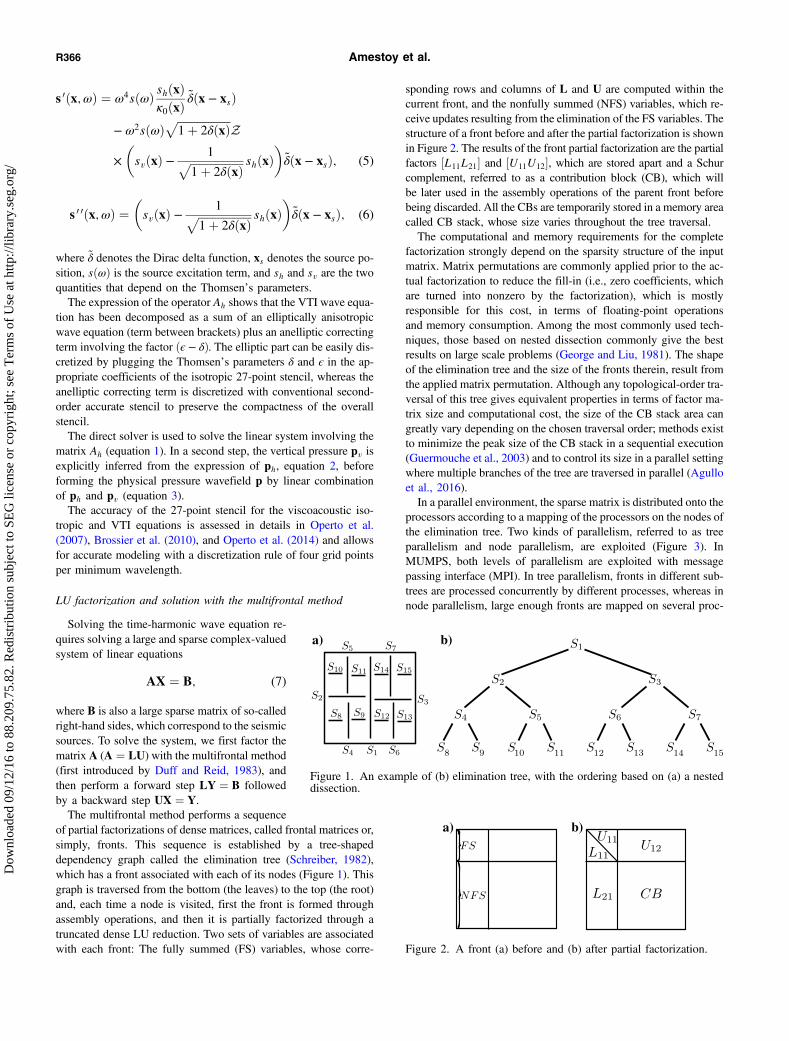
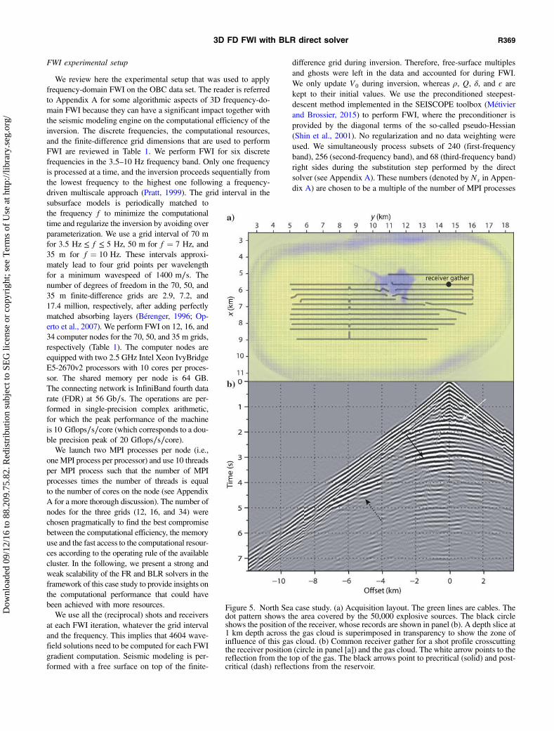
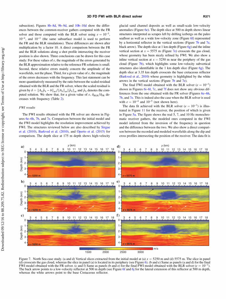
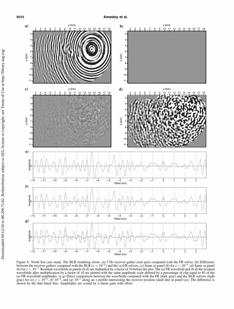
a) b)
c)
e)
f)
g)
d)
y (km)x
(km
)
x (k
m)
x (k
m)
x (k
m)
y (km) y (km)
y (km)
Figure 8 North Sea case study The BLR modeling errors (a) 5 Hz receiver gather (real part) computed with the FR solver (b) Differencebetween the receiver gathers computed with the BLR (ε frac14 10minus5) and the (a) FR solvers (c) Same as panel (b) for ε frac14 10minus4 (d) Same as panel(b) for ε frac14 10minus3 Residual wavefields in panels (b-d) are multiplied by a factor of 10 before the plot The (a) FR wavefield and (b-d) the residualwavefields after multiplication by a factor of 10 are plotted with the same amplitude scale defined by a percentage of clip equal to 85 of the(a) FR-wavefield amplitudes (e-g) Direct comparison between the wavefields computed with the FR (dark gray) and the BLR solvers (lightgray) for (e) ε frac14 10minus5 (f) 10minus4 and (g) 10minus3 along an x profile intersecting the receiver position (dash line in panel (a)) The difference isshown by the thin black line Amplitudes are scaled by a linear gain with offset
R372 Amestoy et al
Dow
nloa
ded
091
216
to 8
820
975
82
Red
istr
ibut
ion
subj
ect t
o SE
G li
cens
e or
cop
yrig
ht s
ee T
erm
s of
Use
at h
ttp
libra
rys
ego
rg
very similar to the one achieved with the FR solver (not shown heresee Operto et al [2015] their Figures 15ndash17) and is quite satisfac-tory in particular in terms of phase We already noted that the mod-eled amplitudes tend to be overestimated at long offsets when thewavefield has propagated through the gas cloud in the dip directionunlike in the cross direction (Figure 11b ellipse) In Operto et al(2015) we interpret these amplitude mismatches as the footprint ofattenuation whose absorption effects have been underestimatedduring seismic modeling with a uniform Q equal to 200 The misfitfunctions versus the iteration number obtained with the FR andBLR (ε frac14 10minus5 10minus4 and 10minus3) solvers for the six frequenciesare shown in Figure 12 The convergence curves obtained withthe FR and the BLR solvers for ε frac14 10minus4 and 10minus5 are very similarIn contrast we show that the convergence achieved by the BLRsolver with ε frac14 10minus3 is alternatively better (4 and 5 Hz) and worse(35 and 45 Hz) than for the three other FWI run when the inversionjumps from one frequency to the next within the 35ndash5 Hzfrequency band However for the last two frequencies (7 and10 Hz) that have the best signal-to-noise ratio all of the four con-vergence curves show a similar trend and reach a similar misfitfunction value at the last iteration This suggests that the crude stop-ping criterion of iteration that is used in this study by fixing acommon maximum iteration count is reasonable for a fair compari-son of the computational cost of each FWI run The different con-vergence behavior at low frequencies shown for ε frac14 10minus3 probablyreflects the sensitivity of the inversion to the noise introduced by theBLR approximation at low frequencies (Figure 8) although thisnoise remains sufficiently weak to not alter the FWI results Thehigher footprint of the BLR approximation at low frequencies dur-ing FWI is consistent with the former analysis of the relative mod-eling errors which decrease as frequency increases (Table 2ratio δBLR∕δFR)
Computational cost
The reduction of the size of the LU factorsoperation count and factorization time obtainedwith the BLR approximation are outlined in Ta-ble 3 for the 5 7 and 10 Hz frequencies respec-tively Compared with the FR factorization thesize of the LU factors obtained with the BLRsolver (ε frac14 10minus3) decreases by a factor of 2630 and 35 for the 5 7 and 10 Hz frequenciesrespectively (field FSLU in Table 3) This can beconverted to a reduction of the memory demand(ongoing work) Moreover the number of flopsduring the LU factorization (field FLU in Table 3)
decreases by factors of 8 107 and 133 when the BLR solver isused The increase of the computational saving achieved by theBLR solver when the problem size grows is further supportedby the weak scalability analysis shown in the next subsection Whenthe BLR solver (ε frac14 10minus3) is used the LU factorization time is de-creased by a factor of 19 27 and 27 with respect to the FR solverfor the 5 7 and 10 Hz frequencies respectively (field TLU inTable 3) The time reduction achieved by the BLR solver tendsto increase with the frequency This trend is also due to the increaseof the workload per MPI process as the frequency increases In-creasing the workload per processor which in our case was guidedby memory constraints tends to favor the parallel performance ofthe BLR solverAs mentioned above the BLR solver does not fully exploit the
compression potential when multithread BLAS kernels are usedbecause low-rank matrices are smaller by nature than originalFR blocks This was confirmed experimentally on the 7 Hz problemwith ε frac14 10minus3 by a computational time reduced by a factor 23 on160 cores even though the flops are reduced by a factor of 111 (thisis not reported in the tables) Adding OpenMP-based parallelismallows us to retrieve a substantial part of this potential reachinga speedup of 38 In comparison with the timings reported by Ames-toy et al (2015c) the performance gains obtained by exploiting thesparsity of the right sides and the improved multithreading are ap-proximately equal to a factor of 23 The elapsed time to computeone wavefield once the LU factorization has been performed issmall (field Ts in Table 3) The two numbers provided in Table 3for Ts are associated with the computation of the incident and ad-joint wavefields In the latter case the source vectors are far lesssparse which leads to a computational overhead during the solutionphase These results in an elapsed time of respectively 262 598and 1542 s to compute the 4604 wavefields required for the com-putation of one FWI gradient (field Tms in Table 3) Despite the high
Table 1 North Sea case study Problem size and computational resources (for the results of Tables 3 and 4 only) hm gridinterval nPML number of grid points in absorbing perfectly matched layers u106 number of unknowns n number ofcomputer nodes MPI number of MPI process th number of threads per MPI process c number of cores and RHS numberof right sides processed per FWI gradient
Frequencies (Hz) HethmTHORN Grid dimensions nPML u n MPI th c RHS
35 4 45 5 70 66 times 130 times 230 8 29 12 24 10 240 4604
7 50 92 times 181 times 321 8 72 16 32 10 320 4604
10 35 131 times 258 times 458 4 174 34 68 10 680 4604
Table 2 North Sea case study Modeling error introduced by BLR for differentlow-rank threshold ε and different frequencies F Here δ scaled residualsdefined as kAh ~ph minus bkinfin∕kAhkinfink~phkinfin for b being for one of the RHS in BThe numbers in parentheses are δBLR∕δFR Note that for a given ε this ratiodecreases as frequency increases
FethHzTHORN∕hethmTHORN δethFRTHORN δethBLR ε frac14 10minus5THORN δethBLR ε frac14 10minus4THORN δethBLR ε frac14 10minus3THORN
5 Hz∕70 m 23 times 10minus7eth1THORN 46 times 10minus6eth20THORN 67 times 10minus5eth291THORN 53 times 10minus4eth2292THORN7 Hz∕50 m 75 times 10minus7eth1THORN 46 times 10minus6eth6THORN 69 times 10minus5eth92THORN 75 times 10minus4eth1000THORN10 Hz∕35 m 13 times 10minus6eth1THORN 29 times 10minus6eth23THORN 30 times 10minus5eth23THORN 43 times 10minus4eth331THORN
3D FD FWI with BLR direct solver R373
Dow
nloa
ded
091
216
to 8
820
975
82
Red
istr
ibut
ion
subj
ect t
o SE
G li
cens
e or
cop
yrig
ht s
ee T
erm
s of
Use
at h
ttp
libra
rys
ego
rg
a) b)
d)c)
e)
f)
g)
y (km)
y (km)
x (k
m)
x (k
m)
x (k
m)
x (k
m)
y (km)
y (km)
Figure 9 North Sea case study The BLRmodeling errors Same as Figure 8 for the 7 Hz frequency The simulations are performed in the samesubsurface model obtained after a 7 Hz inversion (not shown here) The same percentage of clip (85) of the FR-wavefield amplitudes and thesame amplitude scaling of the residuals wavefields (multiplication by a factor of 10 before plot) as those used in Figure 8 are used for plot
R374 Amestoy et al
Dow
nloa
ded
091
216
to 8
820
975
82
Red
istr
ibut
ion
subj
ect t
o SE
G li
cens
e or
cop
yrig
ht s
ee T
erm
s of
Use
at h
ttp
libra
rys
ego
rg
a)
c) d)
e)
f)
g)
b)y (km)
y (km) y (km)
x (k
m)
x (k
m)
x (k
m)
x (k
m)
y (km)
Figure 10 North Sea case study The BLR modeling errors Same as Figure 8 for the 10 Hz frequency The simulations are performed in thesame subsurface model obtained after a 10 Hz inversion The same percentage of clip (85) of the FR-wavefield amplitudes and the sameamplitude scaling of the residuals wavefields (multiplication by a factor of 10 before plot) as those used in Figure 8 are used for plot
3D FD FWI with BLR direct solver R375
Dow
nloa
ded
091
216
to 8
820
975
82
Red
istr
ibut
ion
subj
ect t
o SE
G li
cens
e or
cop
yrig
ht s
ee T
erm
s of
Use
at h
ttp
libra
rys
ego
rg
Figure 11 North Sea case study Data fit achieved with the BLR solver (ε frac14 10minus3) (a) 5 (b) 7 and (c) 10 Hz frequencies Left (x-y) panelshows the recorded data Middle panel shows the modeled data computed in the FWI model inferred from the inversion of the current fre-quency Right panel is the difference Bottom and right amplitude-offset panels show a direct comparison between the recorded (black) and themodeled (gray) data (real part) along a dip and across profiles intersecting the receiver position (dash lines in (x-y) panels) Amplitudes arecorrected for geometric spreading The ellipse delineates an offset range for which modeled amplitudes are overestimated (see text for in-terpretation)
R376 Amestoy et al
Dow
nloa
ded
091
216
to 8
820
975
82
Red
istr
ibut
ion
subj
ect t
o SE
G li
cens
e or
cop
yrig
ht s
ee T
erm
s of
Use
at h
ttp
libra
rys
ego
rg
efficiency of the substitution step the elapsed time required to com-pute the wavefield solutions by substitution (262 598 and 1542 s)is significantly higher than the time required to perform the LU fac-torization (41 121 and 424 s with the BLR solver ε frac14 10minus3) whenall the (reciprocal) sources are processed at each FWI iterationHowever the rate of increase of the solution step is smaller thanthe linear increase of the factor size and factorization time whenincreasing the frequency In other words the real-time complexityof the LU factorization is higher than that of the solution phasealthough the theoretical time complexities are the same for N2 rightsides ethOethN6THORNTHORN This is shown by the decrease of the ratio Tms∕TLU
as the problem size increases (34 186 and 134 for the 70 50 and35 m grids respectively when the FR solver is used) The fact thatthe speedup of the factorization phase achieved by the BLRapproximation increases with the problem size will balance thehigher complexity of the LU factorization relative to the solutionphase and help to address large-scale problems As reported in col-
umn TgethmnTHORN of Table 3 the elapsed times required to compute onegradient with the FR solver are of the order of 99 212 and 69 minfor the 5 7 and 10 Hz frequencies respectively whereas those withthe BLR solver are of the order of 91 171 and 495 min respec-tively Please note that FR and BLR timings already include theacceleration due to the exploitation of the sparsity of the right sidesThus the difference between these two times reflects the computa-tional saving achieved by the BLR approximation during the LUfactorization because the BLR approximation is currently exploitedonly during this taskFor a fair assessment of the FWI speedup provided by the BLR
solver it is also important to check the impact of the BLR approxi-mation on the line search and hence the number of FWI gradientscomputed during FWI (Table 4) On the 70 m grid where the impactof the BLR errors is expected to be the largest one (as indicated inTable 2) the inversion with the BLR solver (ε frac14 10minus3) computes82 gradients against 77 gradients for the three other settings
a)
b)
c) f)
e)
d)
35 Hz
4 Hz
45 Hz
5 Hz
7 Hz
10 Hz
Figure 12 North Sea case study Misfit function versus iteration number achieved with the FR (black cross) and the BLR solvers with ε frac1410minus5 (dark gray triangle) 10minus4 (gray square) and 10minus3 (light gray circle) (a) 35 (b) 4 (c) 45 (d) 5 (e) 7 and (f) 10 Hz inversion
3D FD FWI with BLR direct solver R377
Dow
nloa
ded
091
216
to 8
820
975
82
Red
istr
ibut
ion
subj
ect t
o SE
G li
cens
e or
cop
yrig
ht s
ee T
erm
s of
Use
at h
ttp
libra
rys
ego
rg
(FR and BLR solvers with ε frac14 10minus4 and 10minus5) for a total of 70 FWIiterations On the 7 Hz grid the FR and the BLR solvers withε frac14 10minus5 compute 39 gradients against 30 gradients with the BLRsolver with ε frac14 10minus4 and 10minus3 for a total of 20 FWI iterations Onthe 10 Hz grid the four inversions compute 16 gradients for a totalof 10 FWI iterationsThe elapsed time to perform the FWI is provided for each grid in
Table 4 The entire FWI application takes 492 394 36 and 378 hwith the FR solver and the BLR solver with ε frac14 10minus5 10minus4 and10minus3 respectively We remind that the FWI application performedwith the BLR solver with ε frac14 10minus3 takes more time than with ε frac1410minus4 because more gradients were computed on the 70 m grid Weconclude from this analysis that for this case study the BLR solverwith ε frac14 10minus4 provides the best trade-off between the number ofFWI gradients required to reach a given value of the misfit functionand the computational cost of one gradient computation at low fre-quencies At the 7 and 10 Hz frequencies the BLR solver withε frac14 10minus3 provides the smaller computational cost without impact-ing the quality of the FWI results
Strong and weak scalability of the block low-rank mul-tifrontal solver
We now present a weak and strong scalability analysis of the FRand BLR solvers using the FWI subsurface models described in theprevious sectionsFor the strong scalability analysis we use a subsurface model that
has been obtained by FWI for the 7 Hz frequency It is reminded thatthe grid spacing is 50 m leading to 72 million unknowns in thelinear system (Table 1) We perform seismic modeling in this modelwith the FR and BLR (ε frac14 10minus3) solvers by multiplying by a factorof two the number of cores from one run to the next 40 80 160320 and 640 cores (Table 5 and Figure 13) Therefore the idealacceleration from one configuration to the next is two (represented
by the dashed lines in Figure 13) We obtain an average accelerationof 15 and 14 with the FR and BLR solvers respectively The scal-ability of the FR solver is satisfactory on 320 cores (speedup of 18from 160 to 320 cores Table 5) The 7 Hz matrix is however toosmall to provide enough parallelism and thus we only reach aspeedup of 14 from 320 to 640 cores Moreover we show in Fig-ure 13 that the difference between the FR and BLR execution timesdecreases as the number of cores increases because the BLR solverperforms fewer flops with a smaller granularity than the FR solverand thus the relative weight of communications and noncomputa-tional tasks (eg memory copies and assembly) becomes more im-portant in BLR Indeed although the elapsed time for the FR LUfactorization is 39 times higher than the one for the BLR LU fac-torization when 40 cores are used this ratio decreases to 3 on 320cores and 27 on 640 cores Therefore the strong scalability of theFR solver and the efficiency of the BLR solver relative to the FRsolver should be taken into account when choosing the computa-tional resources that are used for an application Finally the flopcompression rate achieved by BLR is provided in Figure 13 ontop of each point It has the desirable property to remain roughlyconstant when the number of processes grows ie the BLR com-pression does not degrade on higher core countsAweak scalability analysis is shown in Table 6 to assess the com-
putational saving achieved by the BLR solver when the problemsize (ie the frequency) grows We used three matrices generatedfrom subsurface models obtained by FWI for the 5 7 and 10 Hzfrequencies For these three frequencies the grid interval is 70 50and 35 m leading to 29 72 and 174 million of unknowns respec-tively (Table 1) The BLR threshold is set to ε frac14 10minus3 The numberof MPI processes is chosen to keep the memory demand of the LUfactorization per processor of the order of 15 GB This leads to 620 and 64 MPI processes and to 11 times 1013 21 times 1013 and 41 times1013 flopsMPI process (for the FR solver) for the 5 7 and 10 Hzmatrices respectively Because the number of flops per MPI process
Table 3 North Sea case study Computational savings provided by the BLR solver during the factorization step Factor ofimprovement due to BLR is indicated between parentheses The elapsed times required to perform the multi-RHS substitutionstep and to compute the gradient are also provided FSLUGB size of LU factors (GigaBytes) FLU flops for the LUfactorization TLUs elapsed time for the LU factorization Tss average time for one solution The first and second numbersare related to the incident and adjoint wavefields respectively The acceleration from the exploitation of the RHS sparsity isincluded Also Tmss elapsed time for 4604 solutions (incident + adjoint wavefields) Tgmn elapsed time to compute the FWIgradient This time also includes the IO tasks
FethHzTHORN∕hethmTHORN ε FSLUethGBTHORN FLUethtimes1012THORN TLUethsTHORN TsethsTHORN TmsethsTHORN TgethmnTHORN
5 Hz∕70 m (240 cores) FR 62 (10) 66 (10) 78 (10) 00510063 262 99
10minus5 35 (18) 17 (38) 48 (16) 94
10minus4 30 (21) 12 (53) 46 (17) 91
10minus3 24 (26) 8 (80) 41 (19) 91
7 Hz∕50 m (320 cores) FR 211 (10) 410 (10) 322 (10) 012014 598 212
10minus5 90 (23) 90 (45) 157 (21) 177
10minus4 88 (24) 63 (65) 136 (24) 173
10minus3 70 (30) 38 (107) 121 (27) 171
10 Hz∕35 m (680 cores) FR 722 (10) 2600 (10) 1153 (10) 026041 1542 690
10minus5 333 (22) 520 (49) 503 (23) 486
10minus4 271 (27) 340 (75) 442 (26) 489
10minus3 209 (35) 190 (133) 424 (27) 495
R378 Amestoy et al
Dow
nloa
ded
091
216
to 8
820
975
82
Red
istr
ibut
ion
subj
ect t
o SE
G li
cens
e or
cop
yrig
ht s
ee T
erm
s of
Use
at h
ttp
libra
rys
ego
rg
grows in this parallel configuration the execution time increaseswith the matrix size accordingly (Table 6) This allows the FR fac-torization to maintain a high Gflops∕s∕core on higher core counts(52 41 and 35 Gflopsscore respectively to compare with apeak of 10 Gflops∕s∕core) which corresponds to a parallel effi-ciency (normalized with respect to the 5 Hz problem) of 080and 069 for the 7 and 10 Hz problems In comparison the normal-ized efficiency of the BLR factorization is 072 and 052 for the 7and 10 Hz problems Even though the efficiency decreases slightlyfaster in BLR than in FR the flop reduction due to BLR also in-creases with the frequency (124 90 and 73 respectively)which in the end leads to a time reduction by a factor of 27 34 and35 respectively Thus even though the flop reduction is not fullytranslated into time this weak scaling study shows that the gain dueto BLR can be maintained on higher core counts with a significantreduction factor of the order of three in time for the current BLRimplementation
DISCUSSION
We have shown that 3D viscoacoustic VTI fre-quency-domain FWI allows for efficiently build-ing a subsurface model from stationary recordingsystems such as OBC with limited computa-tional resources when the linear system resultingfrom the discretization of the time-harmonicwave equation is solved with a sparse directsolver Two key ingredients in the direct solverwere implemented to achieve high computationalperformance for FWI application The first oneexploits the low-rank properties of the ellipticpartial differential operators embedded in thetime-harmonic wave equation that allows us toreduce the cost of the LU factorization by a factorof approximately three in terms of computationtime and factor size the second one exploits thesparsity of the seismic source vectors to speed upthe forward elimination step during the compu-tation of the solutions Note that the BLRapproximation has so far been implemented inthe LU factorization only ie the FR uncom-pressed LU factors are still used to computethe wavefield solutions by substitution There-fore there is a potential to accelerate the solutionstep once the compression of the LU factorsachieved by the BLR approximation is exploitedMore generally we believe that in the context ofthe solution phase with large numbers of right-hand sides there is still much scope for improve-ment to better exploit the parallelism of our targetcomputers We will investigate in priority this is-sue because it is critical In parallel to the workon the theoretical complexity bounds of the BLRfactorization (Amestoy et al 2016b) we are in-vestigating variants of the BLR factorization im-proving its performance and complexity Anotherpossible object of research is the use of BLR as apreconditioner rather than a direct solver Pre-liminary experiments in Weisbecker (2013) showpromising results although the time to solve
(Ts in Table 3) which is the bottleneck in this applicative contextwould be multiplied by the number of iterationsThe choice of the low-rank threshold is performed by trial and
error However the analysis of the modeling errors introduced bythe BLR approximation and their impact on the convergence behav-ior of the FWI support that the BLR approximation has a strongerfootprint at low frequencies for a given subsurface target Thereforea general strategy might be to use a slightly more accurate factori-zation (smaller ε) at low frequencies when the FWI is not expensiveand use a slightly more aggressive thresholding (higher ε) at higherfrequencies For the case study presented here a value of ε frac14 10minus3
does not impact upon the quality of the FWI results at least at the 7and 10 Hz frequencies Another case study (not shown here) per-formed with a smaller target a portion of the 3D SEGEAGE landoverthrust model shows a stronger footprint of the BLR approxi-mation in the FWI results for ε frac14 10minus3 Additional work is still nec-essary to estimate in a more automated way the optimal choice of εFurthermore the influence of the frequency on the error (FR and
Table 4 North Sea case study The FWI cost it and g are the number of FWIiterations and the number of gradients computed on each grid TFWI is theelapsed time for FWI on each grid The total times for the FWI application are492 394 36 and 378 h for the FR BLR10minus5 BLR10minus4 and BLR10minus3solvers respectively
hethmTHORN Frequency (Hz) c ε it g TFWI (h)
70 35 4 45 5 240 FR 70 77 140
10minus5 70 77 129
10minus4 70 77 127
10minus3 70 82 140
50 7 320 FR 20 39 145
10minus5 20 39 120
10minus4 20 30 91
10minus3 20 30 90
35 10 680 FR 10 16 207
10minus5 10 16 145
10minus4 10 16 142
10minus3 10 16 148
Table 5 North Sea case study Strong scaling analysis of the factorization ofthe 7 Hz problem For BLR the threshold is set to ε 10minus3 AccFRLR(X rarr 2X) is the acceleration factor (ie ratio of time X and over time 2X)obtained by doubling the number of processes See also Figure 13
Time (s) Time (s) Ratio AccFR AccLR
FR BLR FRBLR (X rarr 2X) (X rarr 2X)
4 times 10 1323 336 39 15 14
8 times 10 865 241 36 15 16
16 times 10 574 151 38 18 14
32 times 10 327 110 30 14 13
64 times 10 237 87 27 mdash mdash
3D FD FWI with BLR direct solver R379
Dow
nloa
ded
091
216
to 8
820
975
82
Red
istr
ibut
ion
subj
ect t
o SE
G li
cens
e or
cop
yrig
ht s
ee T
erm
s of
Use
at h
ttp
libra
rys
ego
rg
with BLR) deserves to be more thoroughly investigated from anexperimental and a theoretical standpoint
CONCLUSION
Although 3D frequency-domain FWI based on sparse directmethods is generally considered intractable we have shown in thisstudy its high computational efficiency to process OBC data in theviscoacoustic VTI approximation with quite limited computationalresources The computational efficiency of the frequency-domainFWI relies on a suitable choice of a few discrete frequencies andrecent methodological advances in the development of massivelyparallel sparse multifrontal solver The first advance exploits somelow-rank properties of the elliptic partial differential operators em-bedded in the time harmonic wave equation which allows for asignificant reduction in operation count and computation time dur-ing the LU factorization This compression procedure based on theso-called BLR format and the related approximation should lead toa speedup of the solution step too although this is not yet imple-mented The second advance exploits the sparsity of the right sidesnamely the seismic source vectors to speed up the forward elimi-
nation step during the wavefield computations All these featureslead to a quite efficient computation of wavefield solutions by sub-stitution once the LU factorization has been performed at a veryreasonable cost This offers a suitable framework to preserve thefold resulting from dense seismic acquisitions during the stack pro-cedure underlying FWI and hence build subsurface model with ahigh signal-to-noise ratio Although the FWI was limited to a maxi-mum frequency of 10 Hz it is probably reasonable to try to push theinversion up to a frequency of 15 Hz in the near future For thecase study presented here this would require managing computa-tional grids with up to 60 million of unknowns On the other handalthough the frequency decimation underlying efficient frequency-domain FWI is relatively neutral for monoparameter FWI the im-pact of this decimation will have to be assessed with care in theframework of multiparameter reconstruction This comment how-ever also applies to time-domain FWI which is generally applied toa quite narrow frequency bandwidth Frequency-domain FWI re-mains limited to a relatively narrow range of applications in termsof wave physics and acquisition geometries Extension of our finite-difference stencil to tilted transverse isotropy (TTI) is not straight-forward and should lead to a significant computational overheadApplication to short-spread narrow-azimuth streamer data mightnot be beneficial because the cost of the LU factorizations mightbecome prohibitive relative to one of the solution steps and the num-ber of frequencies to be managed should be increased to preventwraparound artifacts Despite these limitations 3D frequency-domain FWI on OBC data based on a sparse direct solver can alsobe viewed as an efficient tool to build an initial viscoacoustic VTIsubsurface model for subsequent elastic FWI of multicomponentdata Feasibility of frequency-domain viscoelastic modeling basedon sparse direct solver for multicomponentmultiparameter FWI ap-plications at low frequencies needs to be assessed and will be theaim of future work
ACKNOWLEDGMENTS
This study was partly funded by the SEISCOPE consortiumhttpseiscope2osugfr This study was granted access to thehigh-performance computing facilities of the SIGAMM (Observa-toire de la Cocircte drsquoAzur) and the HPC resources of CINESIDRISunder the allocation 046091 made by GENCI We also thank BPNorge AS and their Valhall partner Hess Norge AS for allowingaccess to the Valhall data set as well as the well-log velocitiesWe thank J Virieux (ISTERRE) for his reading of the manuscriptWe thank the associate editor A Guitton J de la Puente J D De
Figure 13 North Sea case study Strong scaling analysis on the7 Hz problem For BLR the threshold is set to ε frac14 10minus3 The valuesnext to the markers show the flops compression rate with respect tothe FR factorization See also Table 5
Table 6 North Sea case study Weak scaling analysis of the factorization on the 5 7 and 10 Hz problems For BLR thethreshold is set to ε 10minus3 The normalized efficiency is the parallel efficiency normalized with respect to the 5 Hz problem runon 6 x 10 cores The peak is 10 Gflops∕s∕core
Time (s) Ratio Flops FR Flops Gflops∕s∕coreNormalizedefficiency
FR BLR FRBLR (times1012) BLRFR FR BLR FR BLR
5 Hzeth6 times 10THORN 210 77 27 66 124 52 18 1 1
7 Hzeth20 times 10THORN 489 144 34 420 90 41 13 080 072
10 Hzeth64 times 10THORN 1132 324 35 2624 73 35 09 069 052
R380 Amestoy et al
Dow
nloa
ded
091
216
to 8
820
975
82
Red
istr
ibut
ion
subj
ect t
o SE
G li
cens
e or
cop
yrig
ht s
ee T
erm
s of
Use
at h
ttp
libra
rys
ego
rg
Basabe and three anonymous reviewers for their constructive com-ments which contributed to the improvement of the manuscript
APPENDIX A
ALGORITHMIC ASPECTS OF FREQUENCY-DOMAIN FWI
The frequency-domain FWI is implemented with the SEISCOPEoptimization toolbox which relies on a reverse-communication inter-face with the user (Meacutetivier and Brossier 2015) The SEISCOPE op-timization toolbox contains several optimization algorithms such assteepest-descent conjugate gradient limited-memory quasi Newtonand truncated Newton optimization as well as a line search that guar-antees that the Wolfe conditions are satisfied during the estimation ofthe step length (Nocedal and Wright 2006) The descent direction pro-vided by each of these optimization algorithms can be improved by apreconditioner provided by the user For the most basic steepest-descentoptimization the user provides to the optimization toolbox the currentsubsurface model the misfit function computed in this model and itsgradient In this study the misfit function is the usual least-squaresnorm of the difference between the recorded and the modeled mono-chromatic data The gradient is computed with the adjoint-state methodthat requires seismic modeling twice per (reciprocal) source (Plessix2006) The gradient of the misfit function for the VTI time-harmonicwave equation is developed in Operto et al (2015) and is given by
nablaCm frac14 R
partAh
partmph
dagger
a1
(A-1)
where the dagger indicates adjoint operator and adjoint wavefield a1satisfies
Ah a1 frac141
3ethAv thorn 2ITHORNRtΔd (A-2)
In equation A-2Δd are the data residualsR denotes the real partof a complex number I is the identity matrix and Rt is a prolon-gation operator which augments with zeros the data residual vectorin the full computational domain (Pratt et al 1998)After the LU factorization of Ah the LU factors are stored in
main memory in distributed form We then sequentially processNa partitions of Ns seismic sources (Ns is the number of columnsin matrix B equation 7) TheNs right-hand sides are built in parallelby distributing them over the processors before their centralizationon the master process with sparse storage The seismic sources arepositioned in the finite-difference grids with a windowed sinc pa-rameterization (Hicks 2002) The solution step performed byMUMPS returns the Ns monochromatic wavefields in distributedform following a domain decomposition driven by the distributionof the LU factors each processor stores a subdomain of the Ns
wavefields Because the domain decomposition is driven by theLU factorization it is unstructured with subdomains of quite hetero-geneous sizes (Sourbier et al [2009] their Figure 2) Therefore it isinefficient for parallel gradient computation as it would lead to anunbalanced workload Moreover a domain decomposition of thegradient would complicate unnecessarily the implementation ofthe radiation pattern matrices partAh∕partm (equation A-1) for secondaryparameters as density and Thomsenrsquos parameters as well as regu-
larizations We therefore chose to redistribute the Ns wavefieldsover the processors according to the source index to implement anembarrassing MPI parallelism over sources Each processor storesthe full domain of Ns∕Np wavefields where Np denotes the num-ber of MPI processNext we interpolate the values of the incident wavefields at the
receiver positions with the windowed sinc parameterization (Hicks2002) followed by the estimation of the source signature (Pratt1999) and the update of the misfit function The source signatureis averaged over the sources involved in the current partition Thesame modeling workflow is applied to process the adjoint wave-fields All along the process the Ns incident and adjoint wavefieldsremain in random-access memory (RAM) in distributed form ac-cording to the source index The gradient of the misfit functioncan then be updated quite efficiently by combining the embarrass-ing parallelism over sources with shared-memory parallelism toprocess the degrees of freedom of the gradient grid The gradientalgorithm is above-described for one frequency When several fre-quency components are simultaneously inverted the multifre-quency gradient is the sum of each monofrequency gradient Theouter loop over frequencies in the FWI algorithm can be either proc-essed sequentially or in parallel with an additional MPI communi-cator if enough computational resources are availableA suitable architecture for frequency-domain FWI should take ad-
vantage of multicore central processing units (CPUs) with a signifi-cant amount of RAM This significant amount of RAM allows for thesimultaneous processing of a large number of right-hand sides in thematrix B (equation 7) taking advantage of multithreaded BLAS3 ker-nels and the sparsity of the source vectors Note that because we canafford to keep in the core the incident wavefields all along the com-putation they do not need to be recomputed during the adjoint sim-ulation and the gradient computation a distinct advantage comparedwith the time-domain implementation To limit memory overheadsand volume of communication during the LU factorization we typ-ically assign only one MPI process per socket or CPU each MPIprocess being multithreaded over the cores of its CPU This matchesthe architecture best ensuring a uniform memory access within eachMPI process and in our experience provides in general comparableor better performance during LU factorization and solving than usinga single MPI process per node
REFERENCES
Agullo E P R Amestoy A Buttari A Guermouche J-Y LrsquoExcellent andF-H Rouet 2016 Robust memory-aware mappings for parallel multi-frontal factorizations SIAM Journal on Scientific Computing 38C256ndashC279
Amestoy P R J Anton C Ashcraft A Buttari P Ghysels J-Y LrsquoExcel-lent X S Li T Mary F-H Rouet and C Weisbecker 2016a A com-parison of parallel rank-structured solvers Presented at the SIAMConference on Parallel Processing
Amestoy P R C Ashcraft O Boiteau A Buttari J-Y LrsquoExcellent and CWeisbecker 2015a Improving multifrontal methods by means of blocklow-rank representations SIAM Journal on Scientific Computing 37A1451ndashA1474 doi 101137120903476
Amestoy P R A Buttari J-Y LrsquoExcellent and T Mary 2016b Complex-ity and performance of the block low-rank multifrontal factorization Pre-sented at the SIAM Conference on Parallel Processing SIAM PP16
Amestoy P R R Brossier A Buttari J-Y LrsquoExcellent T Mary L Meacute-tivier A Miniussi S Operto J Virieux and C Weisbecker 2015b 3Dfrequency-domain seismic modeling with a parallel BLR multifrontal di-rect solver 85th Annual International Meeting SEG Expanded Ab-stracts 3606ndash3611
Amestoy P R R Brossier A Buttari J-Y LrsquoExcellent T Mary L Meacute-tivier A Miniussi S Operto A Ribodetti J Virieux and C Weisbecker2015c Efficient 3D frequency-domain full-waveform inversion of ocean-
3D FD FWI with BLR direct solver R381
Dow
nloa
ded
091
216
to 8
820
975
82
Red
istr
ibut
ion
subj
ect t
o SE
G li
cens
e or
cop
yrig
ht s
ee T
erm
s of
Use
at h
ttp
libra
rys
ego
rg
bottom cable data with sparse block low-rank direct solver A real datacase study from the North Sea 85th Annual International Meeting SEGExpanded Abstracts 1303ndash1308
Amestoy P R I S Duff J-Y LrsquoExcellent and F-H Rouet 2015d Parallelcomputation of entries of Aminus1 SIAM Journal on Scientific Computing37 C268ndashC284 doi 101137120902616
Amestoy P R I S Duff J Koster and J-Y LrsquoExcellent 2001 A fullyasynchronous multifrontal solver using distributed dynamic schedulingSIAM Journal on Matrix Analysis and Applications 23 15ndash41 doi101137S0895479899358194
Amestoy P R A Guermouche J-Y LrsquoExcellent and S Pralet 2006 Hy-brid scheduling for the parallel solution of linear systems Parallel Com-puting 32 136ndash156 doi 101016jparco200507004
Aminfar A and E Darve 2016 A fast memory efficient and robust sparsepreconditioner based on a multifrontal approach with applications to fi-nite-element matrices International Journal for Numerical Methods inEngineering 107 520ndash540
Barkved O U Albertin P Heavey J Kommedal J van Gestel R Syn-nove H Pettersen and C Kent 2010 Business impact of full waveforminversion at Valhall 91st Annual International Meeting and ExpositionSEG Expanded Abstracts 925ndash929
Barnes C and M Charara 2009 The domain of applicability of acousticfull-waveform inversion for marine seismic data Geophysics 74 no 6WCC91ndashWCC103 doi 10119013250269
Bebendorf M 2004 Efficient inversion of the Galerkin matrix ofgeneral second-order elliptic operators with nonsmooth coefficientsMathematics of Computation 74 1179ndash1200 doi 101090S0025-5718-04-01716-8
Ben Hadj Ali H S Operto and J Virieux 2008 Velocity model buildingby 3D frequency-domain full-waveform inversion of wide-aperture seis-mic data Geophysics 73 no 5 VE101ndashVE117 doi 10119012957948
Beacuterenger J P 1996 Three-dimensional perfectly matched layer for the ab-sorption of electromagnetic waves Journal of Computational Physics127 363ndash379 doi 101006jcph19960181
Brossier R V Etienne S Operto and J Virieux 2010 Frequency-domainnumerical modeling of visco-acoustic waves based on finite-differenceand finite-element discontinuous Galerkin methods in D W Dissa-nayake ed Acoustic waves INTECH 125ndash158
Castagna J P M L Batzle and T K Kan 1993 Rock physics mdash Thelink between rock properties and AVO response in J P Castagna and MM Backus eds Offset-dependent reflectivity-theory and practice ofAVO analysis SEG
Coleman T and C vanLoan 1988 Handbook of matrix computationsSIAM
Duff I S and J K Reid 1983 The multifrontal solution of indefinitesparse symmetric linear systems ACM Transactions on MathematicalSoftware 9 302ndash325 doi 101145356044356047
Erlangga Y A and R Nabben 2008 On a multilevel Krylov method forthe Helmholtz equation preconditioned by shifted Laplacian ElectronicTransactions on Numerical Analysis 31 403ndash424
George A and J W Liu 1981 Computer solution of large sparse positivedefinite systems Prentice-Hall Inc
Ghysels P X S Li F Rouet S Williams and A Napov 2015 An efficientmulti-core implementation of a novel HSS-structured multifrontal solverusing randomized sampling CoRR httparxivorgabs150207405v1accessed 29 August 2016
Gilbert J R and J W Liu 1993 Elimination structures for unsymmetricsparse LU factors SIAM Journal on Matrix Analysis and Applications14 334ndash352 doi 1011370614024
Gosselin-Cliche B and B Giroux 2014 3D frequency-domain finite-dif-ference viscoelastic-wave modeling using weighted average 27-point op-erators with optimal coefficients Geophysics 79 no 3 T169ndashT188 doi101190geo2013-03681
Guermouche A J-Y LrsquoExcellent and G Utard 2003 Impact of reorderingon the memory of a multifrontal solver Parallel Computing 29 1191ndash1218 doi 101016S0167-8191(03)00099-1
Hackbusch W 1999 A sparse matrix arithmetic based on H-matrices PartI Introduction to H-matrices Computing 62 89ndash108 doi 101007s006070050015
Hicks G J 2002 Arbitrary source and receiver positioning in finite-differ-ence schemes using Kaiser windowed sinc functions Geophysics 67156ndash165 doi 10119011451454
Hustedt B S Operto and J Virieux 2004 Mixed-grid and staggered-gridfinite difference methods for frequency domain acoustic wave modellingGeophysical Journal International 157 1269ndash1296 doi 101111j1365-246X200402289x
Jo C H C Shin and J H Suh 1996 An optimal 9-point finite-differencefrequency-space 2D scalar extrapolator Geophysics 61 529ndash537 doi 10119011443979
Krebs J J Anderson D Hinkley R Neelamani S Lee A Baumstein andM D Lacasse 2009 Fast full-wavefield seismic inversion using encoded
sources Geophysics 74 no 6 WCC105ndashWCC116 doi 10119013230502
Li Y L Meacutetivier R Brossier B Han and J Virieux 2015 2D and 3Dfrequency-domain elastic wave modeling in complex media with a paral-lel iterative solver Geophysics 80 no 3 T101ndashT118 doi 101190geo2014-04801
Marfurt K 1984 Accuracy of finite-difference and finite-element modelingof the scalar and elastic wave equations Geophysics 49 533ndash549 doi 10119011441689
Meacutetivier L and R Brossier 2015 The SEISCOPE optimization toolbox Alarge-scale nonlinear optimization library based on reverse communica-tion Geophysics 81 no 2 F1ndashF15 doi 101190geo2015-00311
Min D J C Sin B-D Kwon and S Chung 2000 Improved frequency-domain elastic wave modeling using weighted-averaging difference oper-ators Geophysics 65 884ndash895 doi 10119011444785
MUMPS team 2015 MUMPS mdash Multifrontal massively parallel solverusersrsquo guide mdash version 500 httpwwwmumps-solverorg accessed20 February 2015
Nihei K T and X Li 2007 Frequency response modelling of seismicwaves using finite difference time domain with phase sensitive detection(TD-PSD) Geophysical Journal International 169 1069ndash1078 doi 101111j1365-246X200603262x
Nocedal J and S J Wright 2006 Numerical optimization 2nd ed SpringerOperto S R Brossier L Combe L Meacutetivier A Ribodetti and J Virieux
2014 Computationally efficient three-dimensional visco-acoustic finite-difference frequency-domain seismic modeling in vertical transverselyisotropic media with sparse direct solver Geophysics 79 no 5T257ndashT275 doi 101190geo2013-04781
Operto S A Miniussi R Brossier L Combe L Meacutetivier V Monteiller ARibodetti and J Virieux 2015 Efficient 3-D frequency-domain mono-parameter full-waveform inversion of ocean-bottom cable data Applicationto Valhall in the viscoacoustic vertical transverse isotropic approximationGeophysical Journal International 202 1362ndash1391 doi 101093gjiggv226
Operto S J Virieux P R Amestoy J-Y LrsquoExcellent L Giraud and HBen Hadj Ali 2007 3D finite-difference frequency-domain modeling ofvisco-acoustic wave propagation using a massively parallel direct solverA feasibility study Geophysics 72 no 5 SM195ndashSM211 doi 10119012759835
Petrov P V and G A Newman 2012 3D finite-difference modeling ofelastic wave propagation in the Laplace-Fourier domain Geophysics77 no 4 T137ndashT155 doi 101190geo2011-02381
Petrov P V and G A Newman 2014 Three-dimensional inverse modelingof damped elastic wave propagation in the Fourier domain GeophysicalJournal International 198 1599ndash1617 doi 101093gjiggu222
Plessix R E 2006 A review of the adjoint-state method for computing thegradient of a functional with geophysical applications Geophysical JournalInternational 167 495ndash503 doi 101111j1365-246X200602978x
Plessix R E 2007 A Helmholtz iterative solver for 3D seismic-imagingproblems Geophysics 72 no 5 SM185ndashSM194 doi 10119012738849
Plessix R E 2009 Three-dimensional frequency-domain full-waveforminversion with an iterative solver Geophysics 74 no 6 WCC53ndashWCC61 doi 10119013211198
Plessix R-E and C Perez Solano 2015 Modified surface boundary con-ditions for elastic waveform inversion of low-frequency wide-angle activeland seismic data Geophysical Journal International 201 1324ndash1334doi 101093gjiggv087
Pratt R G 1999 Seismic waveform inversion in the frequency domainPart I Theory and verification in a physic scale model Geophysics64 888ndash901 doi 10119011444597
Pratt R G C Shin and G J Hicks 1998 Gauss-Newton and full Newtonmethods in frequency-space seismic waveform inversion Geophysical Jour-nal International 133 341ndash362 doi 101046j1365-246X199800498x
Pratt R G and M H Worthington 1990 Inverse theory applied to multi-source cross-hole tomography Part I Acoustic wave-equation methodGeophysical Prospecting 38 287ndash310 doi 101111j1365-24781990tb01846x
Prieux V R Brossier Y Gholami S Operto J Virieux O Barkved and JKommedal 2011 On the footprint of anisotropy on isotropic full wave-form inversion The Valhall case study Geophysical Journal International187 1495ndash1515 doi 101111j1365-246X201105209x
Prieux V R Brossier S Operto and J Virieux 2013a Multiparameter fullwaveform inversion of multicomponent OBC data from Valhall Part 1Imaging compressional wavespeed density and attenuation GeophysicalJournal International 194 1640ndash1664 doi 101093gjiggt177
Prieux V R Brossier S Operto and J Virieux 2013b Multiparameter fullwaveform inversion of multicomponent OBC data from Valhall Part 2Imaging compressional and shear-wave velocities Geophysical JournalInternational 194 1665ndash1681 doi 101093gjiggt178
Riyanti C D Y A Erlangga R E Plessix W A Mulder C Vuik and COosterlee 2006 A new iterative solver for the time-harmonic wave equa-tion Geophysics 71 no 5 E57ndashE63 doi 10119012231109
R382 Amestoy et al
Dow
nloa
ded
091
216
to 8
820
975
82
Red
istr
ibut
ion
subj
ect t
o SE
G li
cens
e or
cop
yrig
ht s
ee T
erm
s of
Use
at h
ttp
libra
rys
ego
rg
Rouet F X S Li P Ghysels and A Napov 2015 A distributed-memorypackage for dense hierarchically semi-separable matrix computations us-ing randomization CoRR
Schreiber R 1982 A new implementation of sparse Gaussian eliminationACM Transactions on Mathematical Software 8 256ndash276 doi 101145356004356006
Shin C S Jang and D J Min 2001 Improved amplitude preservation forprestack depth migration by inverse scattering theory Geophysical Pro-specting 49 592ndash606 doi 101046j1365-2478200100279x
Sirgue L and R G Pratt 2004 Efficient waveform inversion and imagingA strategy for selecting temporal frequencies Geophysics 69 231ndash248doi 10119011649391
Sirgue L O I Barkved J Dellinger J Etgen U Albertin and J H Kom-medal 2010 Full waveform inversion The next leap forward in imagingat Valhall First Break 28 65ndash70 doi 1039971365-23972010012
Sirgue L J T Etgen and U Albertin 2008 3D frequency domain waveforminversion using time domain finite difference methods 70th AnnualInternational Conference and Exhibition EAGE Extended Abstracts F022
Sourbier F A Haiddar L Giraud H Ben-Hadj-Ali S Operto and J Vir-ieux 2011 Three-dimensional parallel frequency-domain visco-acousticwave modelling based on a hybrid directiterative solver GeophysicalProspecting 59 834ndash856 doi 101111j1365-2478201100966x
Sourbier F S Operto J Virieux P R Amestoy and J-Y LrsquoExcellent2009 FWT2D A massively parallel program for frequency-domainfull-waveform tomography of wide-aperture seismic data mdash Part 1 Al-gorithm Computers amp Geosciences 35 487ndash495 doi 101016jcageo200804013
Stekl I and R G Pratt 1998 Accurate viscoelastic modeling by fre-quency-domain finite difference using rotated operators Geophysics63 1779ndash1794 doi 10119011444472
Tarantola A 1984 Inversion of seismic reflection data in the acousticapproximation Geophysics 49 1259ndash1266 doi 10119011441754
Vigh D and E W Starr 2008a 3D prestack plane-wave full waveforminversion Geophysics 73 no 5 VE135ndashVE144 doi 10119012952623
Vigh D and E W Starr 2008b Comparisons for waveform inversion timedomain or frequency domain 78th Annual International Meeting SEGExpanded Abstracts 1890ndash1894
Virieux J and S Operto 2009 An overview of full waveform inversion inexploration geophysics Geophysics 74 no 6 WCC1ndashWCC26 doi 10119013238367
Wang S M V de Hoop and J Xia 2011 On 3Dmodeling of seismic wavepropagation via a structured parallel multifrontal direct Helmholtz solverGeophysical Prospecting 59 857ndash873 doi 101111j1365-2478201100982x
Wang S M V de Hoop J Xia and X S Li 2012a Massively parallelstructured multifrontal solver for time-harmonic elastic waves in 3Danisotropic media Geophysical Journal International 191 346ndash366doi 101111j1365-246X201205634x
Wang S J Xia M V de Hoop and X S Li 2012b Massively parallelstructured direct solver for equations describing time-harmonic qP-polar-ized waves in TTI media Geophysics 77 no 3 T69ndashT82 doi 101190geo2011-01631
Warner M A Ratcliffe T Nangoo J Morgan A Umpleby N Shah VVinje I Stekl L Guasch C Win G Conroy and A Bertrand 2013Anisotropic 3D full-waveform inversion Geophysics 78 no 2 R59ndashR80 doi 101190geo2012-03381
Weisbecker C 2013 Improving multifrontal solvers by means of algebraicblock low-rank representations PhD thesis Toulouse University
Xia J 2013 Randomized sparse direct solvers SIAM Journal on MatrixAnalysis and Applications 34 197ndash227 doi 10113712087116X
Xia J S Chandrasekaran M Gu and X S Li 2009 Superfast multifrontalmethod for large structured linear systems of equations SIAM Journal onMatrix Analysis and Applications 31 1382ndash1411 doi 10113709074543X
3D FD FWI with BLR direct solver R383
Dow
nloa
ded
091
216
to 8
820
975
82
Red
istr
ibut
ion
subj
ect t
o SE
G li
cens
e or
cop
yrig
ht s
ee T
erm
s of
Use
at h
ttp
libra
rys
ego
rg
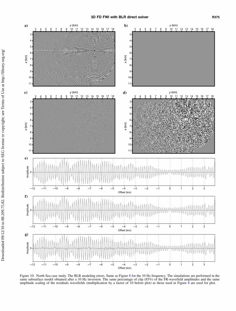
a)
c) d)
e)
f)
g)
b)y (km)
y (km) y (km)
x (k
m)
x (k
m)
x (k
m)
x (k
m)
y (km)
Figure 10 North Sea case study The BLR modeling errors Same as Figure 8 for the 10 Hz frequency The simulations are performed in thesame subsurface model obtained after a 10 Hz inversion The same percentage of clip (85) of the FR-wavefield amplitudes and the sameamplitude scaling of the residuals wavefields (multiplication by a factor of 10 before plot) as those used in Figure 8 are used for plot
3D FD FWI with BLR direct solver R375
Dow
nloa
ded
091
216
to 8
820
975
82
Red
istr
ibut
ion
subj
ect t
o SE
G li
cens
e or
cop
yrig
ht s
ee T
erm
s of
Use
at h
ttp
libra
rys
ego
rg
Figure 11 North Sea case study Data fit achieved with the BLR solver (ε frac14 10minus3) (a) 5 (b) 7 and (c) 10 Hz frequencies Left (x-y) panelshows the recorded data Middle panel shows the modeled data computed in the FWI model inferred from the inversion of the current fre-quency Right panel is the difference Bottom and right amplitude-offset panels show a direct comparison between the recorded (black) and themodeled (gray) data (real part) along a dip and across profiles intersecting the receiver position (dash lines in (x-y) panels) Amplitudes arecorrected for geometric spreading The ellipse delineates an offset range for which modeled amplitudes are overestimated (see text for in-terpretation)
R376 Amestoy et al
Dow
nloa
ded
091
216
to 8
820
975
82
Red
istr
ibut
ion
subj
ect t
o SE
G li
cens
e or
cop
yrig
ht s
ee T
erm
s of
Use
at h
ttp
libra
rys
ego
rg
efficiency of the substitution step the elapsed time required to com-pute the wavefield solutions by substitution (262 598 and 1542 s)is significantly higher than the time required to perform the LU fac-torization (41 121 and 424 s with the BLR solver ε frac14 10minus3) whenall the (reciprocal) sources are processed at each FWI iterationHowever the rate of increase of the solution step is smaller thanthe linear increase of the factor size and factorization time whenincreasing the frequency In other words the real-time complexityof the LU factorization is higher than that of the solution phasealthough the theoretical time complexities are the same for N2 rightsides ethOethN6THORNTHORN This is shown by the decrease of the ratio Tms∕TLU
as the problem size increases (34 186 and 134 for the 70 50 and35 m grids respectively when the FR solver is used) The fact thatthe speedup of the factorization phase achieved by the BLRapproximation increases with the problem size will balance thehigher complexity of the LU factorization relative to the solutionphase and help to address large-scale problems As reported in col-
umn TgethmnTHORN of Table 3 the elapsed times required to compute onegradient with the FR solver are of the order of 99 212 and 69 minfor the 5 7 and 10 Hz frequencies respectively whereas those withthe BLR solver are of the order of 91 171 and 495 min respec-tively Please note that FR and BLR timings already include theacceleration due to the exploitation of the sparsity of the right sidesThus the difference between these two times reflects the computa-tional saving achieved by the BLR approximation during the LUfactorization because the BLR approximation is currently exploitedonly during this taskFor a fair assessment of the FWI speedup provided by the BLR
solver it is also important to check the impact of the BLR approxi-mation on the line search and hence the number of FWI gradientscomputed during FWI (Table 4) On the 70 m grid where the impactof the BLR errors is expected to be the largest one (as indicated inTable 2) the inversion with the BLR solver (ε frac14 10minus3) computes82 gradients against 77 gradients for the three other settings
a)
b)
c) f)
e)
d)
35 Hz
4 Hz
45 Hz
5 Hz
7 Hz
10 Hz
Figure 12 North Sea case study Misfit function versus iteration number achieved with the FR (black cross) and the BLR solvers with ε frac1410minus5 (dark gray triangle) 10minus4 (gray square) and 10minus3 (light gray circle) (a) 35 (b) 4 (c) 45 (d) 5 (e) 7 and (f) 10 Hz inversion
3D FD FWI with BLR direct solver R377
Dow
nloa
ded
091
216
to 8
820
975
82
Red
istr
ibut
ion
subj
ect t
o SE
G li
cens
e or
cop
yrig
ht s
ee T
erm
s of
Use
at h
ttp
libra
rys
ego
rg
(FR and BLR solvers with ε frac14 10minus4 and 10minus5) for a total of 70 FWIiterations On the 7 Hz grid the FR and the BLR solvers withε frac14 10minus5 compute 39 gradients against 30 gradients with the BLRsolver with ε frac14 10minus4 and 10minus3 for a total of 20 FWI iterations Onthe 10 Hz grid the four inversions compute 16 gradients for a totalof 10 FWI iterationsThe elapsed time to perform the FWI is provided for each grid in
Table 4 The entire FWI application takes 492 394 36 and 378 hwith the FR solver and the BLR solver with ε frac14 10minus5 10minus4 and10minus3 respectively We remind that the FWI application performedwith the BLR solver with ε frac14 10minus3 takes more time than with ε frac1410minus4 because more gradients were computed on the 70 m grid Weconclude from this analysis that for this case study the BLR solverwith ε frac14 10minus4 provides the best trade-off between the number ofFWI gradients required to reach a given value of the misfit functionand the computational cost of one gradient computation at low fre-quencies At the 7 and 10 Hz frequencies the BLR solver withε frac14 10minus3 provides the smaller computational cost without impact-ing the quality of the FWI results
Strong and weak scalability of the block low-rank mul-tifrontal solver
We now present a weak and strong scalability analysis of the FRand BLR solvers using the FWI subsurface models described in theprevious sectionsFor the strong scalability analysis we use a subsurface model that
has been obtained by FWI for the 7 Hz frequency It is reminded thatthe grid spacing is 50 m leading to 72 million unknowns in thelinear system (Table 1) We perform seismic modeling in this modelwith the FR and BLR (ε frac14 10minus3) solvers by multiplying by a factorof two the number of cores from one run to the next 40 80 160320 and 640 cores (Table 5 and Figure 13) Therefore the idealacceleration from one configuration to the next is two (represented
by the dashed lines in Figure 13) We obtain an average accelerationof 15 and 14 with the FR and BLR solvers respectively The scal-ability of the FR solver is satisfactory on 320 cores (speedup of 18from 160 to 320 cores Table 5) The 7 Hz matrix is however toosmall to provide enough parallelism and thus we only reach aspeedup of 14 from 320 to 640 cores Moreover we show in Fig-ure 13 that the difference between the FR and BLR execution timesdecreases as the number of cores increases because the BLR solverperforms fewer flops with a smaller granularity than the FR solverand thus the relative weight of communications and noncomputa-tional tasks (eg memory copies and assembly) becomes more im-portant in BLR Indeed although the elapsed time for the FR LUfactorization is 39 times higher than the one for the BLR LU fac-torization when 40 cores are used this ratio decreases to 3 on 320cores and 27 on 640 cores Therefore the strong scalability of theFR solver and the efficiency of the BLR solver relative to the FRsolver should be taken into account when choosing the computa-tional resources that are used for an application Finally the flopcompression rate achieved by BLR is provided in Figure 13 ontop of each point It has the desirable property to remain roughlyconstant when the number of processes grows ie the BLR com-pression does not degrade on higher core countsAweak scalability analysis is shown in Table 6 to assess the com-
putational saving achieved by the BLR solver when the problemsize (ie the frequency) grows We used three matrices generatedfrom subsurface models obtained by FWI for the 5 7 and 10 Hzfrequencies For these three frequencies the grid interval is 70 50and 35 m leading to 29 72 and 174 million of unknowns respec-tively (Table 1) The BLR threshold is set to ε frac14 10minus3 The numberof MPI processes is chosen to keep the memory demand of the LUfactorization per processor of the order of 15 GB This leads to 620 and 64 MPI processes and to 11 times 1013 21 times 1013 and 41 times1013 flopsMPI process (for the FR solver) for the 5 7 and 10 Hzmatrices respectively Because the number of flops per MPI process
Table 3 North Sea case study Computational savings provided by the BLR solver during the factorization step Factor ofimprovement due to BLR is indicated between parentheses The elapsed times required to perform the multi-RHS substitutionstep and to compute the gradient are also provided FSLUGB size of LU factors (GigaBytes) FLU flops for the LUfactorization TLUs elapsed time for the LU factorization Tss average time for one solution The first and second numbersare related to the incident and adjoint wavefields respectively The acceleration from the exploitation of the RHS sparsity isincluded Also Tmss elapsed time for 4604 solutions (incident + adjoint wavefields) Tgmn elapsed time to compute the FWIgradient This time also includes the IO tasks
FethHzTHORN∕hethmTHORN ε FSLUethGBTHORN FLUethtimes1012THORN TLUethsTHORN TsethsTHORN TmsethsTHORN TgethmnTHORN
5 Hz∕70 m (240 cores) FR 62 (10) 66 (10) 78 (10) 00510063 262 99
10minus5 35 (18) 17 (38) 48 (16) 94
10minus4 30 (21) 12 (53) 46 (17) 91
10minus3 24 (26) 8 (80) 41 (19) 91
7 Hz∕50 m (320 cores) FR 211 (10) 410 (10) 322 (10) 012014 598 212
10minus5 90 (23) 90 (45) 157 (21) 177
10minus4 88 (24) 63 (65) 136 (24) 173
10minus3 70 (30) 38 (107) 121 (27) 171
10 Hz∕35 m (680 cores) FR 722 (10) 2600 (10) 1153 (10) 026041 1542 690
10minus5 333 (22) 520 (49) 503 (23) 486
10minus4 271 (27) 340 (75) 442 (26) 489
10minus3 209 (35) 190 (133) 424 (27) 495
R378 Amestoy et al
Dow
nloa
ded
091
216
to 8
820
975
82
Red
istr
ibut
ion
subj
ect t
o SE
G li
cens
e or
cop
yrig
ht s
ee T
erm
s of
Use
at h
ttp
libra
rys
ego
rg
grows in this parallel configuration the execution time increaseswith the matrix size accordingly (Table 6) This allows the FR fac-torization to maintain a high Gflops∕s∕core on higher core counts(52 41 and 35 Gflopsscore respectively to compare with apeak of 10 Gflops∕s∕core) which corresponds to a parallel effi-ciency (normalized with respect to the 5 Hz problem) of 080and 069 for the 7 and 10 Hz problems In comparison the normal-ized efficiency of the BLR factorization is 072 and 052 for the 7and 10 Hz problems Even though the efficiency decreases slightlyfaster in BLR than in FR the flop reduction due to BLR also in-creases with the frequency (124 90 and 73 respectively)which in the end leads to a time reduction by a factor of 27 34 and35 respectively Thus even though the flop reduction is not fullytranslated into time this weak scaling study shows that the gain dueto BLR can be maintained on higher core counts with a significantreduction factor of the order of three in time for the current BLRimplementation
DISCUSSION
We have shown that 3D viscoacoustic VTI fre-quency-domain FWI allows for efficiently build-ing a subsurface model from stationary recordingsystems such as OBC with limited computa-tional resources when the linear system resultingfrom the discretization of the time-harmonicwave equation is solved with a sparse directsolver Two key ingredients in the direct solverwere implemented to achieve high computationalperformance for FWI application The first oneexploits the low-rank properties of the ellipticpartial differential operators embedded in thetime-harmonic wave equation that allows us toreduce the cost of the LU factorization by a factorof approximately three in terms of computationtime and factor size the second one exploits thesparsity of the seismic source vectors to speed upthe forward elimination step during the compu-tation of the solutions Note that the BLRapproximation has so far been implemented inthe LU factorization only ie the FR uncom-pressed LU factors are still used to computethe wavefield solutions by substitution There-fore there is a potential to accelerate the solutionstep once the compression of the LU factorsachieved by the BLR approximation is exploitedMore generally we believe that in the context ofthe solution phase with large numbers of right-hand sides there is still much scope for improve-ment to better exploit the parallelism of our targetcomputers We will investigate in priority this is-sue because it is critical In parallel to the workon the theoretical complexity bounds of the BLRfactorization (Amestoy et al 2016b) we are in-vestigating variants of the BLR factorization im-proving its performance and complexity Anotherpossible object of research is the use of BLR as apreconditioner rather than a direct solver Pre-liminary experiments in Weisbecker (2013) showpromising results although the time to solve
(Ts in Table 3) which is the bottleneck in this applicative contextwould be multiplied by the number of iterationsThe choice of the low-rank threshold is performed by trial and
error However the analysis of the modeling errors introduced bythe BLR approximation and their impact on the convergence behav-ior of the FWI support that the BLR approximation has a strongerfootprint at low frequencies for a given subsurface target Thereforea general strategy might be to use a slightly more accurate factori-zation (smaller ε) at low frequencies when the FWI is not expensiveand use a slightly more aggressive thresholding (higher ε) at higherfrequencies For the case study presented here a value of ε frac14 10minus3
does not impact upon the quality of the FWI results at least at the 7and 10 Hz frequencies Another case study (not shown here) per-formed with a smaller target a portion of the 3D SEGEAGE landoverthrust model shows a stronger footprint of the BLR approxi-mation in the FWI results for ε frac14 10minus3 Additional work is still nec-essary to estimate in a more automated way the optimal choice of εFurthermore the influence of the frequency on the error (FR and
Table 4 North Sea case study The FWI cost it and g are the number of FWIiterations and the number of gradients computed on each grid TFWI is theelapsed time for FWI on each grid The total times for the FWI application are492 394 36 and 378 h for the FR BLR10minus5 BLR10minus4 and BLR10minus3solvers respectively
hethmTHORN Frequency (Hz) c ε it g TFWI (h)
70 35 4 45 5 240 FR 70 77 140
10minus5 70 77 129
10minus4 70 77 127
10minus3 70 82 140
50 7 320 FR 20 39 145
10minus5 20 39 120
10minus4 20 30 91
10minus3 20 30 90
35 10 680 FR 10 16 207
10minus5 10 16 145
10minus4 10 16 142
10minus3 10 16 148
Table 5 North Sea case study Strong scaling analysis of the factorization ofthe 7 Hz problem For BLR the threshold is set to ε 10minus3 AccFRLR(X rarr 2X) is the acceleration factor (ie ratio of time X and over time 2X)obtained by doubling the number of processes See also Figure 13
Time (s) Time (s) Ratio AccFR AccLR
FR BLR FRBLR (X rarr 2X) (X rarr 2X)
4 times 10 1323 336 39 15 14
8 times 10 865 241 36 15 16
16 times 10 574 151 38 18 14
32 times 10 327 110 30 14 13
64 times 10 237 87 27 mdash mdash
3D FD FWI with BLR direct solver R379
Dow
nloa
ded
091
216
to 8
820
975
82
Red
istr
ibut
ion
subj
ect t
o SE
G li
cens
e or
cop
yrig
ht s
ee T
erm
s of
Use
at h
ttp
libra
rys
ego
rg
with BLR) deserves to be more thoroughly investigated from anexperimental and a theoretical standpoint
CONCLUSION
Although 3D frequency-domain FWI based on sparse directmethods is generally considered intractable we have shown in thisstudy its high computational efficiency to process OBC data in theviscoacoustic VTI approximation with quite limited computationalresources The computational efficiency of the frequency-domainFWI relies on a suitable choice of a few discrete frequencies andrecent methodological advances in the development of massivelyparallel sparse multifrontal solver The first advance exploits somelow-rank properties of the elliptic partial differential operators em-bedded in the time harmonic wave equation which allows for asignificant reduction in operation count and computation time dur-ing the LU factorization This compression procedure based on theso-called BLR format and the related approximation should lead toa speedup of the solution step too although this is not yet imple-mented The second advance exploits the sparsity of the right sidesnamely the seismic source vectors to speed up the forward elimi-
nation step during the wavefield computations All these featureslead to a quite efficient computation of wavefield solutions by sub-stitution once the LU factorization has been performed at a veryreasonable cost This offers a suitable framework to preserve thefold resulting from dense seismic acquisitions during the stack pro-cedure underlying FWI and hence build subsurface model with ahigh signal-to-noise ratio Although the FWI was limited to a maxi-mum frequency of 10 Hz it is probably reasonable to try to push theinversion up to a frequency of 15 Hz in the near future For thecase study presented here this would require managing computa-tional grids with up to 60 million of unknowns On the other handalthough the frequency decimation underlying efficient frequency-domain FWI is relatively neutral for monoparameter FWI the im-pact of this decimation will have to be assessed with care in theframework of multiparameter reconstruction This comment how-ever also applies to time-domain FWI which is generally applied toa quite narrow frequency bandwidth Frequency-domain FWI re-mains limited to a relatively narrow range of applications in termsof wave physics and acquisition geometries Extension of our finite-difference stencil to tilted transverse isotropy (TTI) is not straight-forward and should lead to a significant computational overheadApplication to short-spread narrow-azimuth streamer data mightnot be beneficial because the cost of the LU factorizations mightbecome prohibitive relative to one of the solution steps and the num-ber of frequencies to be managed should be increased to preventwraparound artifacts Despite these limitations 3D frequency-domain FWI on OBC data based on a sparse direct solver can alsobe viewed as an efficient tool to build an initial viscoacoustic VTIsubsurface model for subsequent elastic FWI of multicomponentdata Feasibility of frequency-domain viscoelastic modeling basedon sparse direct solver for multicomponentmultiparameter FWI ap-plications at low frequencies needs to be assessed and will be theaim of future work
ACKNOWLEDGMENTS
This study was partly funded by the SEISCOPE consortiumhttpseiscope2osugfr This study was granted access to thehigh-performance computing facilities of the SIGAMM (Observa-toire de la Cocircte drsquoAzur) and the HPC resources of CINESIDRISunder the allocation 046091 made by GENCI We also thank BPNorge AS and their Valhall partner Hess Norge AS for allowingaccess to the Valhall data set as well as the well-log velocitiesWe thank J Virieux (ISTERRE) for his reading of the manuscriptWe thank the associate editor A Guitton J de la Puente J D De
Figure 13 North Sea case study Strong scaling analysis on the7 Hz problem For BLR the threshold is set to ε frac14 10minus3 The valuesnext to the markers show the flops compression rate with respect tothe FR factorization See also Table 5
Table 6 North Sea case study Weak scaling analysis of the factorization on the 5 7 and 10 Hz problems For BLR thethreshold is set to ε 10minus3 The normalized efficiency is the parallel efficiency normalized with respect to the 5 Hz problem runon 6 x 10 cores The peak is 10 Gflops∕s∕core
Time (s) Ratio Flops FR Flops Gflops∕s∕coreNormalizedefficiency
FR BLR FRBLR (times1012) BLRFR FR BLR FR BLR
5 Hzeth6 times 10THORN 210 77 27 66 124 52 18 1 1
7 Hzeth20 times 10THORN 489 144 34 420 90 41 13 080 072
10 Hzeth64 times 10THORN 1132 324 35 2624 73 35 09 069 052
R380 Amestoy et al
Dow
nloa
ded
091
216
to 8
820
975
82
Red
istr
ibut
ion
subj
ect t
o SE
G li
cens
e or
cop
yrig
ht s
ee T
erm
s of
Use
at h
ttp
libra
rys
ego
rg
Basabe and three anonymous reviewers for their constructive com-ments which contributed to the improvement of the manuscript
APPENDIX A
ALGORITHMIC ASPECTS OF FREQUENCY-DOMAIN FWI
The frequency-domain FWI is implemented with the SEISCOPEoptimization toolbox which relies on a reverse-communication inter-face with the user (Meacutetivier and Brossier 2015) The SEISCOPE op-timization toolbox contains several optimization algorithms such assteepest-descent conjugate gradient limited-memory quasi Newtonand truncated Newton optimization as well as a line search that guar-antees that the Wolfe conditions are satisfied during the estimation ofthe step length (Nocedal and Wright 2006) The descent direction pro-vided by each of these optimization algorithms can be improved by apreconditioner provided by the user For the most basic steepest-descentoptimization the user provides to the optimization toolbox the currentsubsurface model the misfit function computed in this model and itsgradient In this study the misfit function is the usual least-squaresnorm of the difference between the recorded and the modeled mono-chromatic data The gradient is computed with the adjoint-state methodthat requires seismic modeling twice per (reciprocal) source (Plessix2006) The gradient of the misfit function for the VTI time-harmonicwave equation is developed in Operto et al (2015) and is given by
nablaCm frac14 R
partAh
partmph
dagger
a1
(A-1)
where the dagger indicates adjoint operator and adjoint wavefield a1satisfies
Ah a1 frac141
3ethAv thorn 2ITHORNRtΔd (A-2)
In equation A-2Δd are the data residualsR denotes the real partof a complex number I is the identity matrix and Rt is a prolon-gation operator which augments with zeros the data residual vectorin the full computational domain (Pratt et al 1998)After the LU factorization of Ah the LU factors are stored in
main memory in distributed form We then sequentially processNa partitions of Ns seismic sources (Ns is the number of columnsin matrix B equation 7) TheNs right-hand sides are built in parallelby distributing them over the processors before their centralizationon the master process with sparse storage The seismic sources arepositioned in the finite-difference grids with a windowed sinc pa-rameterization (Hicks 2002) The solution step performed byMUMPS returns the Ns monochromatic wavefields in distributedform following a domain decomposition driven by the distributionof the LU factors each processor stores a subdomain of the Ns
wavefields Because the domain decomposition is driven by theLU factorization it is unstructured with subdomains of quite hetero-geneous sizes (Sourbier et al [2009] their Figure 2) Therefore it isinefficient for parallel gradient computation as it would lead to anunbalanced workload Moreover a domain decomposition of thegradient would complicate unnecessarily the implementation ofthe radiation pattern matrices partAh∕partm (equation A-1) for secondaryparameters as density and Thomsenrsquos parameters as well as regu-
larizations We therefore chose to redistribute the Ns wavefieldsover the processors according to the source index to implement anembarrassing MPI parallelism over sources Each processor storesthe full domain of Ns∕Np wavefields where Np denotes the num-ber of MPI processNext we interpolate the values of the incident wavefields at the
receiver positions with the windowed sinc parameterization (Hicks2002) followed by the estimation of the source signature (Pratt1999) and the update of the misfit function The source signatureis averaged over the sources involved in the current partition Thesame modeling workflow is applied to process the adjoint wave-fields All along the process the Ns incident and adjoint wavefieldsremain in random-access memory (RAM) in distributed form ac-cording to the source index The gradient of the misfit functioncan then be updated quite efficiently by combining the embarrass-ing parallelism over sources with shared-memory parallelism toprocess the degrees of freedom of the gradient grid The gradientalgorithm is above-described for one frequency When several fre-quency components are simultaneously inverted the multifre-quency gradient is the sum of each monofrequency gradient Theouter loop over frequencies in the FWI algorithm can be either proc-essed sequentially or in parallel with an additional MPI communi-cator if enough computational resources are availableA suitable architecture for frequency-domain FWI should take ad-
vantage of multicore central processing units (CPUs) with a signifi-cant amount of RAM This significant amount of RAM allows for thesimultaneous processing of a large number of right-hand sides in thematrix B (equation 7) taking advantage of multithreaded BLAS3 ker-nels and the sparsity of the source vectors Note that because we canafford to keep in the core the incident wavefields all along the com-putation they do not need to be recomputed during the adjoint sim-ulation and the gradient computation a distinct advantage comparedwith the time-domain implementation To limit memory overheadsand volume of communication during the LU factorization we typ-ically assign only one MPI process per socket or CPU each MPIprocess being multithreaded over the cores of its CPU This matchesthe architecture best ensuring a uniform memory access within eachMPI process and in our experience provides in general comparableor better performance during LU factorization and solving than usinga single MPI process per node
REFERENCES
Agullo E P R Amestoy A Buttari A Guermouche J-Y LrsquoExcellent andF-H Rouet 2016 Robust memory-aware mappings for parallel multi-frontal factorizations SIAM Journal on Scientific Computing 38C256ndashC279
Amestoy P R J Anton C Ashcraft A Buttari P Ghysels J-Y LrsquoExcel-lent X S Li T Mary F-H Rouet and C Weisbecker 2016a A com-parison of parallel rank-structured solvers Presented at the SIAMConference on Parallel Processing
Amestoy P R C Ashcraft O Boiteau A Buttari J-Y LrsquoExcellent and CWeisbecker 2015a Improving multifrontal methods by means of blocklow-rank representations SIAM Journal on Scientific Computing 37A1451ndashA1474 doi 101137120903476
Amestoy P R A Buttari J-Y LrsquoExcellent and T Mary 2016b Complex-ity and performance of the block low-rank multifrontal factorization Pre-sented at the SIAM Conference on Parallel Processing SIAM PP16
Amestoy P R R Brossier A Buttari J-Y LrsquoExcellent T Mary L Meacute-tivier A Miniussi S Operto J Virieux and C Weisbecker 2015b 3Dfrequency-domain seismic modeling with a parallel BLR multifrontal di-rect solver 85th Annual International Meeting SEG Expanded Ab-stracts 3606ndash3611
Amestoy P R R Brossier A Buttari J-Y LrsquoExcellent T Mary L Meacute-tivier A Miniussi S Operto A Ribodetti J Virieux and C Weisbecker2015c Efficient 3D frequency-domain full-waveform inversion of ocean-
3D FD FWI with BLR direct solver R381
Dow
nloa
ded
091
216
to 8
820
975
82
Red
istr
ibut
ion
subj
ect t
o SE
G li
cens
e or
cop
yrig
ht s
ee T
erm
s of
Use
at h
ttp
libra
rys
ego
rg
bottom cable data with sparse block low-rank direct solver A real datacase study from the North Sea 85th Annual International Meeting SEGExpanded Abstracts 1303ndash1308
Amestoy P R I S Duff J-Y LrsquoExcellent and F-H Rouet 2015d Parallelcomputation of entries of Aminus1 SIAM Journal on Scientific Computing37 C268ndashC284 doi 101137120902616
Amestoy P R I S Duff J Koster and J-Y LrsquoExcellent 2001 A fullyasynchronous multifrontal solver using distributed dynamic schedulingSIAM Journal on Matrix Analysis and Applications 23 15ndash41 doi101137S0895479899358194
Amestoy P R A Guermouche J-Y LrsquoExcellent and S Pralet 2006 Hy-brid scheduling for the parallel solution of linear systems Parallel Com-puting 32 136ndash156 doi 101016jparco200507004
Aminfar A and E Darve 2016 A fast memory efficient and robust sparsepreconditioner based on a multifrontal approach with applications to fi-nite-element matrices International Journal for Numerical Methods inEngineering 107 520ndash540
Barkved O U Albertin P Heavey J Kommedal J van Gestel R Syn-nove H Pettersen and C Kent 2010 Business impact of full waveforminversion at Valhall 91st Annual International Meeting and ExpositionSEG Expanded Abstracts 925ndash929
Barnes C and M Charara 2009 The domain of applicability of acousticfull-waveform inversion for marine seismic data Geophysics 74 no 6WCC91ndashWCC103 doi 10119013250269
Bebendorf M 2004 Efficient inversion of the Galerkin matrix ofgeneral second-order elliptic operators with nonsmooth coefficientsMathematics of Computation 74 1179ndash1200 doi 101090S0025-5718-04-01716-8
Ben Hadj Ali H S Operto and J Virieux 2008 Velocity model buildingby 3D frequency-domain full-waveform inversion of wide-aperture seis-mic data Geophysics 73 no 5 VE101ndashVE117 doi 10119012957948
Beacuterenger J P 1996 Three-dimensional perfectly matched layer for the ab-sorption of electromagnetic waves Journal of Computational Physics127 363ndash379 doi 101006jcph19960181
Brossier R V Etienne S Operto and J Virieux 2010 Frequency-domainnumerical modeling of visco-acoustic waves based on finite-differenceand finite-element discontinuous Galerkin methods in D W Dissa-nayake ed Acoustic waves INTECH 125ndash158
Castagna J P M L Batzle and T K Kan 1993 Rock physics mdash Thelink between rock properties and AVO response in J P Castagna and MM Backus eds Offset-dependent reflectivity-theory and practice ofAVO analysis SEG
Coleman T and C vanLoan 1988 Handbook of matrix computationsSIAM
Duff I S and J K Reid 1983 The multifrontal solution of indefinitesparse symmetric linear systems ACM Transactions on MathematicalSoftware 9 302ndash325 doi 101145356044356047
Erlangga Y A and R Nabben 2008 On a multilevel Krylov method forthe Helmholtz equation preconditioned by shifted Laplacian ElectronicTransactions on Numerical Analysis 31 403ndash424
George A and J W Liu 1981 Computer solution of large sparse positivedefinite systems Prentice-Hall Inc
Ghysels P X S Li F Rouet S Williams and A Napov 2015 An efficientmulti-core implementation of a novel HSS-structured multifrontal solverusing randomized sampling CoRR httparxivorgabs150207405v1accessed 29 August 2016
Gilbert J R and J W Liu 1993 Elimination structures for unsymmetricsparse LU factors SIAM Journal on Matrix Analysis and Applications14 334ndash352 doi 1011370614024
Gosselin-Cliche B and B Giroux 2014 3D frequency-domain finite-dif-ference viscoelastic-wave modeling using weighted average 27-point op-erators with optimal coefficients Geophysics 79 no 3 T169ndashT188 doi101190geo2013-03681
Guermouche A J-Y LrsquoExcellent and G Utard 2003 Impact of reorderingon the memory of a multifrontal solver Parallel Computing 29 1191ndash1218 doi 101016S0167-8191(03)00099-1
Hackbusch W 1999 A sparse matrix arithmetic based on H-matrices PartI Introduction to H-matrices Computing 62 89ndash108 doi 101007s006070050015
Hicks G J 2002 Arbitrary source and receiver positioning in finite-differ-ence schemes using Kaiser windowed sinc functions Geophysics 67156ndash165 doi 10119011451454
Hustedt B S Operto and J Virieux 2004 Mixed-grid and staggered-gridfinite difference methods for frequency domain acoustic wave modellingGeophysical Journal International 157 1269ndash1296 doi 101111j1365-246X200402289x
Jo C H C Shin and J H Suh 1996 An optimal 9-point finite-differencefrequency-space 2D scalar extrapolator Geophysics 61 529ndash537 doi 10119011443979
Krebs J J Anderson D Hinkley R Neelamani S Lee A Baumstein andM D Lacasse 2009 Fast full-wavefield seismic inversion using encoded
sources Geophysics 74 no 6 WCC105ndashWCC116 doi 10119013230502
Li Y L Meacutetivier R Brossier B Han and J Virieux 2015 2D and 3Dfrequency-domain elastic wave modeling in complex media with a paral-lel iterative solver Geophysics 80 no 3 T101ndashT118 doi 101190geo2014-04801
Marfurt K 1984 Accuracy of finite-difference and finite-element modelingof the scalar and elastic wave equations Geophysics 49 533ndash549 doi 10119011441689
Meacutetivier L and R Brossier 2015 The SEISCOPE optimization toolbox Alarge-scale nonlinear optimization library based on reverse communica-tion Geophysics 81 no 2 F1ndashF15 doi 101190geo2015-00311
Min D J C Sin B-D Kwon and S Chung 2000 Improved frequency-domain elastic wave modeling using weighted-averaging difference oper-ators Geophysics 65 884ndash895 doi 10119011444785
MUMPS team 2015 MUMPS mdash Multifrontal massively parallel solverusersrsquo guide mdash version 500 httpwwwmumps-solverorg accessed20 February 2015
Nihei K T and X Li 2007 Frequency response modelling of seismicwaves using finite difference time domain with phase sensitive detection(TD-PSD) Geophysical Journal International 169 1069ndash1078 doi 101111j1365-246X200603262x
Nocedal J and S J Wright 2006 Numerical optimization 2nd ed SpringerOperto S R Brossier L Combe L Meacutetivier A Ribodetti and J Virieux
2014 Computationally efficient three-dimensional visco-acoustic finite-difference frequency-domain seismic modeling in vertical transverselyisotropic media with sparse direct solver Geophysics 79 no 5T257ndashT275 doi 101190geo2013-04781
Operto S A Miniussi R Brossier L Combe L Meacutetivier V Monteiller ARibodetti and J Virieux 2015 Efficient 3-D frequency-domain mono-parameter full-waveform inversion of ocean-bottom cable data Applicationto Valhall in the viscoacoustic vertical transverse isotropic approximationGeophysical Journal International 202 1362ndash1391 doi 101093gjiggv226
Operto S J Virieux P R Amestoy J-Y LrsquoExcellent L Giraud and HBen Hadj Ali 2007 3D finite-difference frequency-domain modeling ofvisco-acoustic wave propagation using a massively parallel direct solverA feasibility study Geophysics 72 no 5 SM195ndashSM211 doi 10119012759835
Petrov P V and G A Newman 2012 3D finite-difference modeling ofelastic wave propagation in the Laplace-Fourier domain Geophysics77 no 4 T137ndashT155 doi 101190geo2011-02381
Petrov P V and G A Newman 2014 Three-dimensional inverse modelingof damped elastic wave propagation in the Fourier domain GeophysicalJournal International 198 1599ndash1617 doi 101093gjiggu222
Plessix R E 2006 A review of the adjoint-state method for computing thegradient of a functional with geophysical applications Geophysical JournalInternational 167 495ndash503 doi 101111j1365-246X200602978x
Plessix R E 2007 A Helmholtz iterative solver for 3D seismic-imagingproblems Geophysics 72 no 5 SM185ndashSM194 doi 10119012738849
Plessix R E 2009 Three-dimensional frequency-domain full-waveforminversion with an iterative solver Geophysics 74 no 6 WCC53ndashWCC61 doi 10119013211198
Plessix R-E and C Perez Solano 2015 Modified surface boundary con-ditions for elastic waveform inversion of low-frequency wide-angle activeland seismic data Geophysical Journal International 201 1324ndash1334doi 101093gjiggv087
Pratt R G 1999 Seismic waveform inversion in the frequency domainPart I Theory and verification in a physic scale model Geophysics64 888ndash901 doi 10119011444597
Pratt R G C Shin and G J Hicks 1998 Gauss-Newton and full Newtonmethods in frequency-space seismic waveform inversion Geophysical Jour-nal International 133 341ndash362 doi 101046j1365-246X199800498x
Pratt R G and M H Worthington 1990 Inverse theory applied to multi-source cross-hole tomography Part I Acoustic wave-equation methodGeophysical Prospecting 38 287ndash310 doi 101111j1365-24781990tb01846x
Prieux V R Brossier Y Gholami S Operto J Virieux O Barkved and JKommedal 2011 On the footprint of anisotropy on isotropic full wave-form inversion The Valhall case study Geophysical Journal International187 1495ndash1515 doi 101111j1365-246X201105209x
Prieux V R Brossier S Operto and J Virieux 2013a Multiparameter fullwaveform inversion of multicomponent OBC data from Valhall Part 1Imaging compressional wavespeed density and attenuation GeophysicalJournal International 194 1640ndash1664 doi 101093gjiggt177
Prieux V R Brossier S Operto and J Virieux 2013b Multiparameter fullwaveform inversion of multicomponent OBC data from Valhall Part 2Imaging compressional and shear-wave velocities Geophysical JournalInternational 194 1665ndash1681 doi 101093gjiggt178
Riyanti C D Y A Erlangga R E Plessix W A Mulder C Vuik and COosterlee 2006 A new iterative solver for the time-harmonic wave equa-tion Geophysics 71 no 5 E57ndashE63 doi 10119012231109
R382 Amestoy et al
Dow
nloa
ded
091
216
to 8
820
975
82
Red
istr
ibut
ion
subj
ect t
o SE
G li
cens
e or
cop
yrig
ht s
ee T
erm
s of
Use
at h
ttp
libra
rys
ego
rg
Rouet F X S Li P Ghysels and A Napov 2015 A distributed-memorypackage for dense hierarchically semi-separable matrix computations us-ing randomization CoRR
Schreiber R 1982 A new implementation of sparse Gaussian eliminationACM Transactions on Mathematical Software 8 256ndash276 doi 101145356004356006
Shin C S Jang and D J Min 2001 Improved amplitude preservation forprestack depth migration by inverse scattering theory Geophysical Pro-specting 49 592ndash606 doi 101046j1365-2478200100279x
Sirgue L and R G Pratt 2004 Efficient waveform inversion and imagingA strategy for selecting temporal frequencies Geophysics 69 231ndash248doi 10119011649391
Sirgue L O I Barkved J Dellinger J Etgen U Albertin and J H Kom-medal 2010 Full waveform inversion The next leap forward in imagingat Valhall First Break 28 65ndash70 doi 1039971365-23972010012
Sirgue L J T Etgen and U Albertin 2008 3D frequency domain waveforminversion using time domain finite difference methods 70th AnnualInternational Conference and Exhibition EAGE Extended Abstracts F022
Sourbier F A Haiddar L Giraud H Ben-Hadj-Ali S Operto and J Vir-ieux 2011 Three-dimensional parallel frequency-domain visco-acousticwave modelling based on a hybrid directiterative solver GeophysicalProspecting 59 834ndash856 doi 101111j1365-2478201100966x
Sourbier F S Operto J Virieux P R Amestoy and J-Y LrsquoExcellent2009 FWT2D A massively parallel program for frequency-domainfull-waveform tomography of wide-aperture seismic data mdash Part 1 Al-gorithm Computers amp Geosciences 35 487ndash495 doi 101016jcageo200804013
Stekl I and R G Pratt 1998 Accurate viscoelastic modeling by fre-quency-domain finite difference using rotated operators Geophysics63 1779ndash1794 doi 10119011444472
Tarantola A 1984 Inversion of seismic reflection data in the acousticapproximation Geophysics 49 1259ndash1266 doi 10119011441754
Vigh D and E W Starr 2008a 3D prestack plane-wave full waveforminversion Geophysics 73 no 5 VE135ndashVE144 doi 10119012952623
Vigh D and E W Starr 2008b Comparisons for waveform inversion timedomain or frequency domain 78th Annual International Meeting SEGExpanded Abstracts 1890ndash1894
Virieux J and S Operto 2009 An overview of full waveform inversion inexploration geophysics Geophysics 74 no 6 WCC1ndashWCC26 doi 10119013238367
Wang S M V de Hoop and J Xia 2011 On 3Dmodeling of seismic wavepropagation via a structured parallel multifrontal direct Helmholtz solverGeophysical Prospecting 59 857ndash873 doi 101111j1365-2478201100982x
Wang S M V de Hoop J Xia and X S Li 2012a Massively parallelstructured multifrontal solver for time-harmonic elastic waves in 3Danisotropic media Geophysical Journal International 191 346ndash366doi 101111j1365-246X201205634x
Wang S J Xia M V de Hoop and X S Li 2012b Massively parallelstructured direct solver for equations describing time-harmonic qP-polar-ized waves in TTI media Geophysics 77 no 3 T69ndashT82 doi 101190geo2011-01631
Warner M A Ratcliffe T Nangoo J Morgan A Umpleby N Shah VVinje I Stekl L Guasch C Win G Conroy and A Bertrand 2013Anisotropic 3D full-waveform inversion Geophysics 78 no 2 R59ndashR80 doi 101190geo2012-03381
Weisbecker C 2013 Improving multifrontal solvers by means of algebraicblock low-rank representations PhD thesis Toulouse University
Xia J 2013 Randomized sparse direct solvers SIAM Journal on MatrixAnalysis and Applications 34 197ndash227 doi 10113712087116X
Xia J S Chandrasekaran M Gu and X S Li 2009 Superfast multifrontalmethod for large structured linear systems of equations SIAM Journal onMatrix Analysis and Applications 31 1382ndash1411 doi 10113709074543X
3D FD FWI with BLR direct solver R383
Dow
nloa
ded
091
216
to 8
820
975
82
Red
istr
ibut
ion
subj
ect t
o SE
G li
cens
e or
cop
yrig
ht s
ee T
erm
s of
Use
at h
ttp
libra
rys
ego
rg
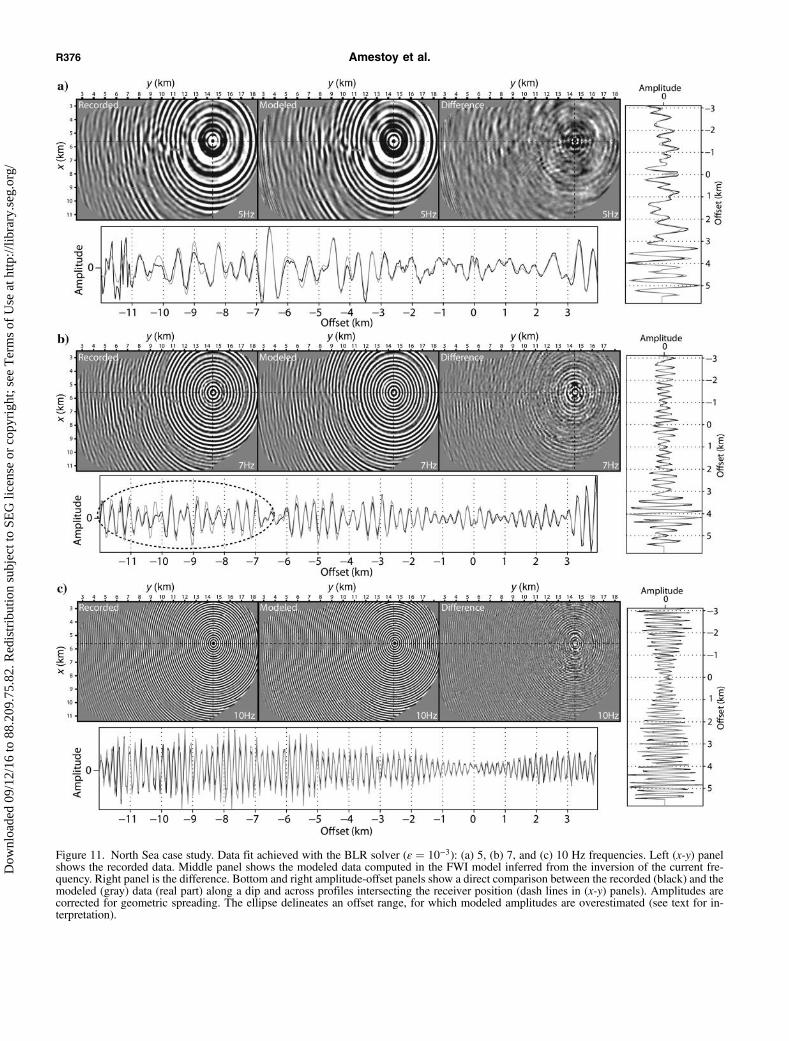
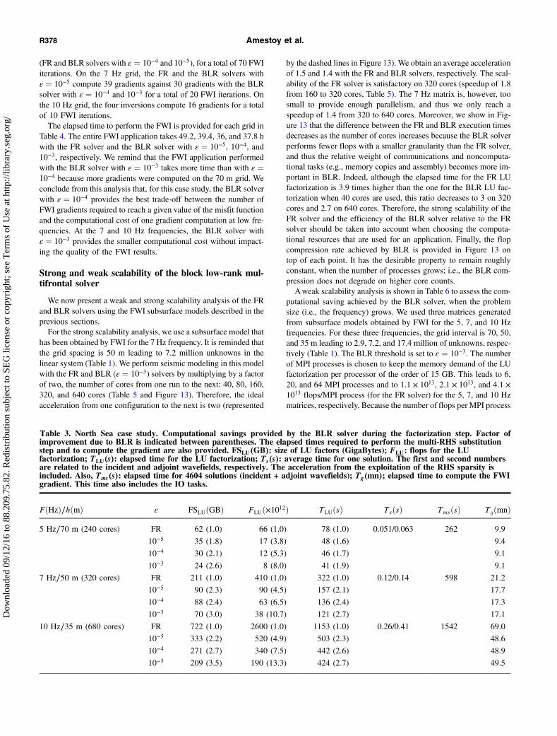
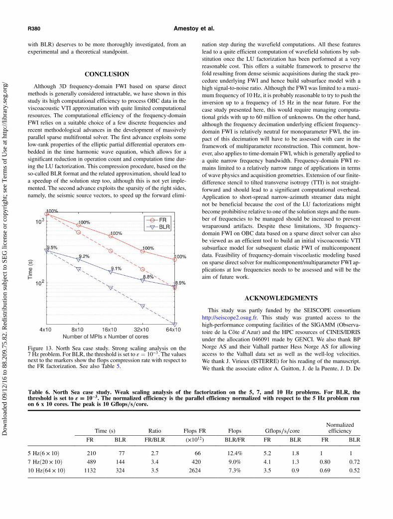


![Ludovic Courtes` [email protected]](https://img.pdfslide.net/doc/110x75/613d439f736caf36b75b4454/ludovic-courtes-emailprotected.jpg)