Embed Size (px)
Citation preview
Fast Adaptive Penalized Splines
Tatyana Krivobokova∗
Katholieke Universiteit LeuvenCiprian M. Crainiceanu†
Johns Hopkins University
Goran Kauermann‡
Universitat Bielefeld
17th April 2007
Abstract
This paper proposes a numerically simple method for locally adaptive smooth-
ing. The heterogeneous regression function is modeled as a penalized spline
with a varying smoothing parameter modeled as another penalized spline.
This is formulated as a hierarchical mixed model, with spline coefficients
following zero mean normal distribution with a smooth variance structure.
The modeling framework is similar to Baladandayuthapani, Mallick & Car-
roll (2005) and Crainiceanu, Ruppert, Carroll, Adarsh & Goodner (2006). In
contrast to these papers the Laplace approximation of the marginal likelihood
is used for estimation. This method is numerically simple and fast. The idea
is extended to spatial and non-normal response smoothing.
Keywords: Function of locally varying complexity; Hierarchical mixed model;
Laplace approximation
∗ORSTAT, K.U. Leuven, Naamsestraat 69 - bus 3555, B-3000 Leuven, Belgium (email:[email protected])
†Department of Biostatistics, Johns Hopkins Bloomberg School of Public Health, 615 N.WolfeSt. E3636 Baltimore, MD 21205 (email: [email protected])
‡Department of Economics, University of Bielefeld, Postfach 100131, 33501 Bielefeld, Germany(email: [email protected])
1

1 Introduction
Penalized spline smoothing has become increasingly popular in recent years. Origi-
nally introduced by O’Sullivan (1986) it was Eilers & Marx (1996) who gave it the
name P-spline smoothing. The idea is quite simple. A smooth unknown regression
function is estimated by assuming a functional parametric shape constructed via a
high dimensional basis function. The dimension of the basis is chosen generously
to achieve the desired flexibility, while the basis coefficients are penalized to ensure
smoothness of the resulting functional estimates. The idea of penalized splines has
led to a powerful and applicable smoothing technique which is demonstrated and
motivated in the book by Ruppert, Wand & Carroll (2003). The actual dimension
of the basis used has little influence on the fit as has been shown in Ruppert (2002)
who concludes that “at most 35 to 40 knots (basis functions) could be recommended
for all sample sizes and for all smooth functions without too many oscillations”.
The penalized spline methodology is particularly appealing because it can be shown
that the penalized spline fit is the Best Linear Unbiased Predictor (BLUP) in a par-
ticular mixed model Wand (2003), Ruppert, Wand & Carroll (2003), Kauermann
(2004). Thus, standard mixed models software can be used for smoothing, see Ngo
& Wand (2004), Crainiceanu, Ruppert & Wand (2005) or Lang & Brezger (2004).
Even though penalized spline smoothing is simple and practical, using a single
penalty parameter may fail to correctly capture the features of functions that ex-
hibit strong heterogeneity. This type of function occurs, for example, in applications
where the signal changes rapidly in some regions while remaining relatively smooth
in others. Regression with strongly heterogenous mean function has been addressed
before in the literature and a number of solutions are available. For kernel based
methods Fan & Gijbels (1995) and Herrmann (1997) may serve as references. For
2

spline smoothing Luo & Wahba (1997) suggested hybrid adaptive splines. The idea
is to replace the n dimensional spline basis, where n is the sample size, by an adap-
tively selected subset of the basis functions. This idea has similarities to adaptive
knot selection for regression splines as suggested in Friedman & Silverman (1989).
An alternative approach is to allow the smoothing parameter to vary locally. Using
a reproducing kernel Hilbert space formulation this has been suggested in Pintore,
Speckman & Holmes (2005) using piecewise constant smoothing parameters. Sim-
ilarly, using the penalized spline idea Ruppert & Carroll (2000) allow the penalty
to act differently for each spline basis, where the smoothing parameters are then
selected using a multivariate generalized cross validation. A similar approach is
suggested in Wood, Jiang & Tanner (2002) working with mixtures of splines in a
fully Bayesian framework.
In this paper, we focus on a framework similar to the one in Ruppert & Carroll (2000)
and achieve spatial adaptivity by imposing a functional structure on the smoothing
parameters. This is in line with Baladandayuthapani, Mallick & Carroll (2005) and
Crainiceanu, Ruppert, Carroll, Adarsh & Goodner (2006) who also estimate the er-
ror process variance function. However, these two papers require the use of Bayesian
MCMC methods and are limited to the case of normal responses. Our paper shows
how the MCMC techniques can be circumvented by simple Laplace approximation.
While this might be viewed as a small step back in terms of methodology, it actually
is a forward leap in terms of numerical simplicity. This allows us to develop fast R
software and extend the methodology to non-normal responses.
The paper is organized in Sections that contain their own comparative simulation
studies. Section 2 introduces our spatially adaptive modeling methodology. Section
3 extends the methods to spatial smoothing. Section 4 generalizes the approach to
3

the non-normal responses and provides an example of adaptive bivariate smoothing
for binary data. Section 5 contains our conclusions.
2 Smoothly varying local penalties for P-spline
regression
2.1 Hierarchical penalty model
We start with the following model
yi ∼ Nm(xi), σ2ε, i = 1, ..., n, (1)
where m(x) is a function modeled as a truncated polynomial spline
m(x) = β0 + β1x + ... + βqxq +
Kb∑s=1
bsx− τ (b)s q
+, (2)
τ(b)1 , ..., τ
(b)Kb
are knots covering the range of xs, and x−τ(b)s q
+ is equal to x−τ(b)s q if
x−τ(b)s > 0 and zero otherwise. The dimension Kb of the basis is chosen generously
and the knots τ(b)s are placed over the range of xs, e.g. at the empirical quantiles of xs.
In practice we follow the suggestion of Ruppert (2002) and set Kb ≥ min(n/4, 40).
The penalized spline approach is to impose a penalty on the coefficients bs in (2).
A standard approach is to minimize the sum of squares plus a quadratic penalty
λbT Db, where λ is the penalty parameter and D is the penalty design matrix. For
truncated polynomials the matrix D is the identity matrix and the penalty is λbT b.
For B-splines the penalty is constructed from differences between neighboring spline
coefficients (see Eilers & Marx, 1996). The methodology presented in this paper
is developed for any type of penalized splines and different basis functions will be
used for illustration. Notational simplicity is our only reason for using truncated
polynomial bases.
An important feature of penalized spline smoothing is its link to linear mixed models.
4
It can be shown that the penalized spline fit is the BLUP in a particular mixed
model. More precisely, in this model b ∼ N(0, σ2bD
−) where b is the vector of spline
coefficients, σ2b = σ2
ε /λ, and D− is a (generalized) inverse of D. For truncated
polynomials D = I and b ∼ N(0, σ2bI). One limitation of this approach is that a
single parameter, σ2b , is used to shrink all the spline coefficients. Because of the
global nature of the smoothing parameter, σ2b , information is borrowed from regions
exhibiting high oscillations to regions without and viceversa. The Doppler curve in
Figure (1) is a typical example of such a complex function. To avoid this pitfall we
allow the coefficients b1, ..., bKbto have different prior variances
bs ∼ N [0, σ2bτ (b)
s ], s = 1, ..., Kb,
and assume that the shrinkage variance process σ2bτ (b)
s is a smooth function mod-
eled as a log penalized spline
σ2bτ (b) = exp[γ0 + γ1τ
(b) + ... + γpτ(b)p
+Kc∑t=1
ctτ (b) − τ(c)t p
+], (3)
where τ(c)1 , ..., τ
(c)Kc
is a second layer of knots covering the range of τ(b)1 , . . . , τ
(b)Kb
. The-
oretically we could have Kc = Kb but in practice we choose Kc much smaller than
Kb. Our hierarchical penalized smoothing model is completed by the shrinkage as-
sumption ct ∼ N(0, σ2c ), t = 1, . . . , Kc, where the variance σ2
c is constant. We now
rewrite the model in matrix form. Let
Y =
y1...
yn
, Xb =
1 . . . xq1
......
1 . . . xqn
, Zb =
x1 − τ
(b)1 q
+ . . . x1 − τ(b)Kbq
+...
...
xn − τ(b)1 q
+ . . . xn − τ(b)Kbq
+
,
β = (β0, . . . , βq)T , and b = (b1, . . . , bKb
)T . We also define
Xc =
1 τ(b)1 . . . τ
(b)p
1...
...
1 τ(b)Kb
. . . τ(b)p
Kb
, Zc =
τ (b)
1 − τ(c)1 p
+ . . . τ (b)1 − τ
(c)Kcp
+...
...
τ (b)Kb− τ
(c)1 p
+ . . . τ (b)Kb− τ
(c)Kcp
+
.
5
Thus, our hierarchical smoothing model can be written as
Y |b, c = Xbβ + Zbb + ε, ε ∼ N(0, σ2ε In),
b|c ∼ N(0, Σb), Σb = diagexp(Xcγ + Zcc),
c ∼ N(0, σ2cIKc). (4)
The marginal likelihood of model (4) is
L(β, γ, σ2ε , σ
2c ) = f(Y ; β, γ, σ2
ε , σ2c )
= (2π)−(n+Kc)
2 σ−nε σ−Kc
c
∫
RKc
exp−g(c)dc, (5)
where
g(c) =1
2log |Vε|+ cT c
2σ2c
+(Y −Xbβ)T V −1
ε (Y −Xbβ)
2σ2ε
,
and Vε = In + ZbΣbZTb /σ2
ε . Note that Σb and Vε depend on c and γ, but this
additional notational burden will be omitted throughout the paper. The integral
in (5) is not available analytically, which explains why other authors chose to use
Bayesian MCMC techniques. In contrast, we use the Laplace approximation, which
is justifiable because Kc and Kb are bounded while sample size n is growing, i.e.
Kc < Kb ¿ n. Thus, the Laplace approximation has an error of order O(n−1)
(see Severini, 2000), which makes it an attractive alternative to simulation based
techniques. The Laplace log-likelihood approximation is, up to a constant,
−2l(β, γ, σ2ε , σ
2c ) ≈ n log σ2
ε + Kc log σ2c + log |Vε(c)|+ log |Icc(c)|
+ cT c/σ2c + (Y −Xbβ)T V −1
ε (c)(Y −Xbβ)/σ2ε , (6)
where c is the solution to
∂g(c)
∂ci
=1
2tr
(V −1
ε
∂Vε
∂ci
)+
ci
σ2c
− 1
2σ2ε
(Y −Xbβ)T V −1ε
∂Vε
∂ci
V −1ε (Y −Xbβ) = 0, (7)
6
Icc(c)ij = E
(∂2g(c)
∂ci∂cj
∣∣∣∣ c
)=
δij
σ2c
+1
2tr
(V −1
ε
∂Vε
∂ci
V −1ε
∂Vε
∂cj
), (8)
and δij is Kronecker’s delta. It is easy to show that the derivative appearing in the
above equations results in ∂Vε/∂ci = Zbdiag(Zc,i)ΣbZTb /σ2
ε , where Zc,i stands for the
ith column of the matrix Zc. The prediction of b is defined by ZTb V −1
ε (y −Xbβ) =
σ2ε Σ
−1b b and tr (V −1
ε ∂Vε/∂c) = ZTc wdf , where wdf is the Kb dimensional vector of
diagonal elements of A := ZTb Zb(σ
2ε Σ
−1b + ZT
b Zb)−1. Thus, (7) and (8) become
∂g(c)
∂c= −1
2ZT
c
(Σ−1
b b2 − wdf
)+
c
σ2c
= 0,
and
Icc(c) = E
(∂2g(c)
∂c∂cT
∣∣∣∣ c
)=
1
2ZT
c diag(vdf )Zc +IKc
σ2c
,
respectively. Here vdf is the Kb dimensional vector of diagonal elements of A2. Note
that dfb =∑Kb
s=1 wdf = 1TKb
wdf is the number of degrees of freedom used for fitting b.
Note that ∂vdf/∂γi = 2diag(A2−A3)diag(Xc,i) with Xc,i as the ith column of the
matrix Xc indicating that the weights vdf vary very slowly as a function of γ. Thus,
using this observation we can estimate γ and c simultaneously using the following
iterated weighted least squares (IWLS) algorithm. If θ = (γT , cT )T the algorithm
starts by setting
θ =1
2
(1
2W T
c diag (vdf )Wc +Dc
σ2c
)−1
W Tc diag (vdf ) u, (9)
where Wc = (Xc, Zc), Dc = diag0(p+1)×(p+1), IKc, and u = Wcθ+diag(v−1df )(Σ−1
b b2−wdf ). Minimizing (6) for fixed θ one obtains
σ2c = cT c/wc
df
β = (XTb V −1
ε (θ)Xb)−1XT
b V −1ε (θ)y, (10)
σ2ε = (y −Xbβ)T V −1
ε (θ)(y −Xbβ)/n,
7

with wcdf = tr(Zcdiag(vdf )Z
Tc I−1
cc /2) and obvious definition for Vε(θ). Finally, we
obtain the estimated best linear unbiased predictor (EBLUP) via
b = ΣbZTb V −1
ε (y −Xbβ)/σ2ε .
The latter steps are standard in linear mixed model methodology. Estimation can
now be carried out using the EM type algorithm (see e.g. Searle, Casella, & Mc-
Culloch, 1992 or Breslow & Clayton, 1993) by iterating between (9) and (10) until
convergence. It should be noted that the estimation consists of two simple steps and
is, therefore, numerically fast. In fact, for n = 1000 the fit is obtained in seconds
on standard computers. In contrast Bayesian MCMC methods (Crainiceanu, Rup-
pert, Carroll, Adarsh & Goodner, 2006 or Baladandayuthapani, Mallick & Carroll,
2005) require more than 10 minutes on similar computers. As we will show in subse-
quent sections our proposed method can be extended to non-normal responses and
is robust to small changes of the model. This allowed us to develop the R package
“AdaptFit” which implements the methodology described in this paper (please see
the Appendix).
2.2 Restricted maximum likelihood
The above results are presented for maximum likelihood estimates. The use of
restricted maximum likelihood (REML) is, however, more common in mixed models
(see Harville, 1977). The restricted maximum log-likelihood for the model (4) is
lR(β, γ, σ2ε , σ
2c ) = l(β, γ, σ2
ε , σ2c )−
1
2log |XT
b V −1ε (c)Xb/σ
2ε |,
with l(β, γ, σ2ε , σ
2c ) as given in (6). The estimation method is similar to the one in
Section 2.1, with the matrix A in wdf and vdf replaced by
AR = A− ZTb V −1
ε Xb(XTb V −1
ε Xb)−1XT
b Zb(ZTb Zb + Σ−1
b σ2ε )−1,
8
and the variance estimate replaced by σ2ε = (y−Xbβ)T V −1
ε (θ)(y−Xbβ)/(n− q−1).
In our performance study the ML and REML methods provided similar results.
2.3 Variance estimation
We denote by m(x)|c = Xbβ+Zbb|c the BLUP of the function m(x)|c = Xbβ+Zbb|c,where β = (XT
b V −1ε Xb)
−1XTb V −1
ε y and b|c = ΣbZTb V −1
ε (y −Xbβ)/σ2ε . In the mixed
model framework the function m(x)|c is random because b is random and m(x)|c is
unbiased for m(x)|c. Thus, confidence intervals for m(x)|c can be obtained from
m(x)−m(x)|c ∼ N [0, Varm(x)−m(x)|c],
where Varm(x) −m(x)|c = σ2ε S(θ) = σ2
ε WbW Tb Wb + σ2
ε Db(θ)−1W Tb with Wb =
(Xb, Zb) and Db(θ) = diag0(q+1)×(q+1), Σ−1b . Using the delta method and unbiased-
ness of m(x)|c one can approximate the unconditional variance by
Varm(x)−m(x) = E[Varm(x)−m(x)|c] + Var[Em(x)−m(x)|c] ≈ σ2ε S(c).
Let m(x)|c = Xbβ + Zbb|c denote the EBLUP obtained from m(x)|c by plugging in
the estimates of variance parameters. This can be used to obtain a plug in estimate
Varm(x)−m(x) ≈ σ2ε S(θ).
The variance estimate can also be justified in the Bayesian framework. Assuming
that the parameters Σb = diagexp(Wcθ) and σ2ε are known, the posterior distri-
bution of m(x) is Nm(x, θ), σ2ε S(θ), where m(x, θ) = S(θ)y. An empirical Bayes
approach would replace the unknown values Σb and σ2ε in the prior by estimates and
then treat these parameters as if they were known. Thus, the approximate posterior
distribution of m(x) is Nm(x, θ), σ2ε S(θ), yielding the same confidence intervals
as the frequentist mixed model approach.
The variance formula is simple but does not account for the estimation variability
9

of θ, the parameters of the shrinkage process. This is the price to pay when using
Laplace’s method instead of a full Bayesian approach. For further discussion we
refer to Morris (1983), Laird & Louis (1987), Kass & Steffey (1989) or Ruppert &
Carroll (2000). To correct for this additional variability, we use the delta-method
correction proposed by Kass & Steffey (1989) and obtain
Varm(x)|y = E[Varm(x)|θ, y] + Var[Em(x)|θ, y]
≈ σ2ε S(θ) +
(∂m(x, θ)
∂θ
∣∣∣∣θ=θ
)T
Var(θ)
(∂m(x, θ)
∂θ
∣∣∣∣θ=θ
).
As estimate of Var(θ) one can use the inverse of the Fisher information matrix Iθθ(θ)
obtained from the last iteration of the estimation algorithm. The derivative in the
last term, ignoring the dependence of σ2ε on θ, is
∂m(x, θ)
∂θi
∣∣∣∣θi=θi
= σ2ε Wb(W
Tb Wb + σ2
ε Db)−1Wc,iDb(W
Tb Wb + σ2
ε Db)−1W T
b y,
with Db = Db(θ) and Wc,i = diag0(q+1)×(q+1),Wc,i, where Wc,i is the i-th column
of the matrix Wc.
2.4 Numerical implementation
Our proposed algorithm is simple and can be presented as a sequence of mixed model
fits using standard mixed effects software:
1. Obtain initial estimates for all parameters from a non-adaptive fit, using any
mixed model software;
2. Get next estimates for θ and σ2c from (9) and (10);
3. Update estimates for the remaining parameters with a mixed model software,
taking the estimated variance matrix Σb = diagexp(Wcθ) into account;
10

4. Iterate between 2 and 3 until convergence.
We implemented this algorithm in the package “AdaptFit” described below. We
compared B-splines of different degrees and penalty orders, quadratic and cubic
truncated polynomials as well as cubic thin plate splines. Although all spline bases
produced almost indistinguishable results, the cubic thin plate splines were slightly
more numerically stable and were preferred in the subsequent simulation studies.
2.5 Simulations and comparisons with other univariatesmoothers
We performed a number of simulations. A particular focus is to compare our results
with those reported in Ruppert & Carroll (2000) and Baladandayuthapani, Mallick
& Carroll (2005). First, for n = 400 x equally spaced on [0, 1] and independent
εi ∼ N(0, 0.22) we examined the regression function
m1(x) =√
x(1− x) sin
2π(1 + 2(9−4j)/5)
x + 2(9−4j)/5
,
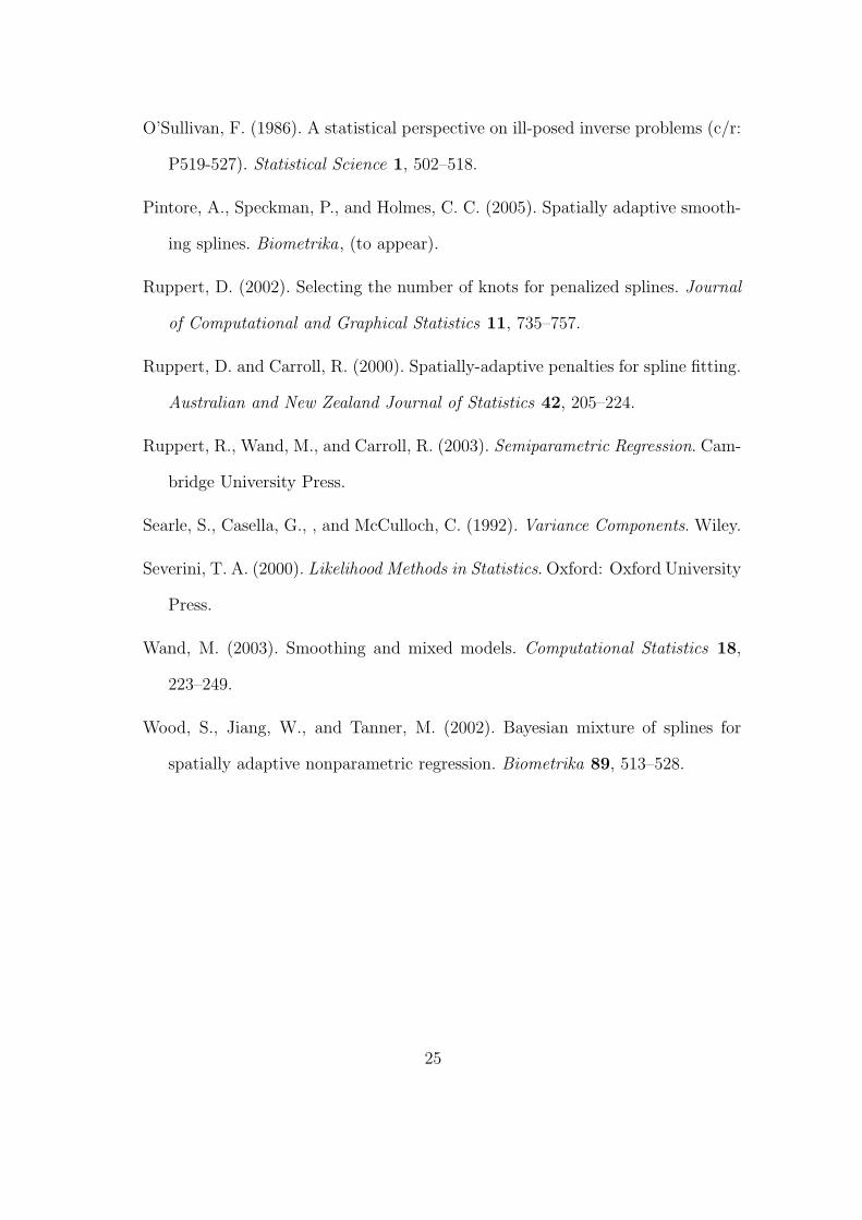
with j = 6. We performed 500 simulations with Kb = 80 and Kc = 20, choosing the
number of knots to be consistent with Ruppert & Carroll (2000). The top plot of
Figure 1 shows the fit and 95% confidence intervals for one simulated data set. The
corresponding estimated variance of random effects is shown in the middle plot. The
average MSE over all x’s obtained as AMSE = n−1∑n
i=1m(xi) −m(xi)2 equals
0.0034, which is comparable with 0.0027 reported in Baladandayuthapani, Mallick
& Carroll (2005) and 0.0026 of Ruppert & Carroll (2000). We also computed the
pointwise coverage probabilities of the 95% confidence intervals over all 500 simu-
lated datasets. The smoothed pointwise coverage probabilities can be seen in the
bottom plot of Figure 1. For small values of x ≤ 0.1, i.e. in the region with low
signal-to-noise ratio, there is clear under-coverage but beyond 0.1 the coverage prob-
11

ability exceeds 95% being slightly conservative. The average coverage probability is
94.95%.
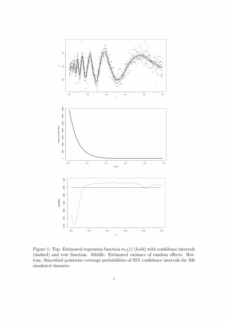
Next, we considered the heterogeneous regression function
m2(x) = exp−400(x− 0.6)2+5
3exp−500(x− 0.75)2+ 2 exp−500(x− 0.9)2,
with n = 1000, the x values being equally spaced on [0, 1] and εi ∼ N(0, 0.52). We
applied our approach to 500 simulated datasets, using Kb = 40 and Kc = 4, following
the choice of Ruppert & Carroll (2000) and Baladandayuthapani, Mallick & Carroll
(2005). The top and middle plots of Figure 2 represent one of the simulated fits and
estimated variance of random effects, respectively. The resulting AMSE is equal
0.0048, which is smaller than 0.0061 and 0.0065, obtained by Baladandayuthapani,
Mallick & Carroll (2005) and Ruppert & Carroll (2000), respectively. The smoothed
pointwise coverage probabilities can be seen in the bottom plot of Figure 2. The av-
erage coverage probability for this function equals 95.94%, which is comparable with
95.22% and 96.28% reported by Baladandayuthapani, Mallick & Carroll (2005) and
Ruppert & Carroll (2000), respectively. For the same setting Baladandayuthapani,
Mallick & Carroll (2005) reported the simulation results for the BARS approach
of DiMatteo, Genovese & Kass (2001). BARS employs free-knots splines with the
random number and location of knots, using reversible jump MCMC for estimation.
The AMSE based on this approach is 0.0043, while the average coverage probability
is 94.72%, both comparable to our approach.
To show the robustness of our approach to the choice of number of subknots Kc, we
performed simulations both for m1(x) and m2(x) with different values of Kc. AMSE
based on 500 simulations for the function m1(x) using 10, 20 and 30 subknots, re-
spectively, resulted in 0.00344025, 0.00344029 and 0.00344023. AMSE based on 500
simulations for the function m2(x) based on Kc equal to 4, 10 and 15, respectively,
12
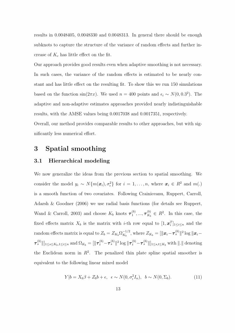
results in 0.0048405, 0.0048330 and 0.0048313. In general there should be enough
subknots to capture the structure of the variance of random effects and further in-
crease of Kc has little effect on the fit.
Our approach provides good results even when adaptive smoothing is not necessary.
In such cases, the variance of the random effects is estimated to be nearly con-
stant and has little effect on the resulting fit. To show this we run 150 simulations
based on the function sin(2πx). We used n = 400 points and εi ∼ N(0, 0.32). The
adaptive and non-adaptive estimates approaches provided nearly indistinguishable
results, with the AMSE values being 0.0017038 and 0.0017351, respectively.
Overall, our method provides comparable results to other approaches, but with sig-
nificantly less numerical effort.
3 Spatial smoothing
3.1 Hierarchical modeling
We now generalize the ideas from the previous section to spatial smoothing. We
consider the model yi ∼ Nm(xi), σ2ε for i = 1, . . . , n, where xi ∈ R2 and m(.)
is a smooth function of two covariates. Following Crainiceanu, Ruppert, Carroll,
Adarsh & Goodner (2006) we use radial basis functions (for details see Ruppert,
Wand & Carroll, 2003) and choose Kb knots τ(b)1 , ..., τ
(b)Kb∈ R2. In this case, the
fixed effects matrix Xb is the matrix with i-th row equal to [1,xTi ]1≤i≤n and the
random effects matrix is equal to Zb = ZKbΩ−1/2Kb
, where ZKb= [‖xi−τ
(b)s ‖2 log ‖xi−
τ(b)s ‖]1≤s≤Kb,1≤i≤n and ΩKb
= [‖τ (b)t −τ
(b)s ‖2 log ‖τ (b)
t −τ(b)s ‖]1≤s,t≤Kb
with ‖.‖ denoting
the Euclidean norm in R2. The penalized thin plate spline spatial smoother is
equivalent to the following linear mixed model
Y |b = Xbβ + Zbb + ε, ε ∼ N(0, σ2ε In), b ∼ N(0, Σb). (11)
13

As in the case of univariate smoothers, local adaptiveness is achieved by allowing
the coefficients b to have spatially variable smoothing parameters. As in Section
2, we set spatial subknots τ(c)1 , ..., τ
(c)Kc
∈ R2, Kc < Kb and define matrices Xc
and Zc similarly to the corresponding definition of matrices Xb and Zb. More pre-
cisely, Xsc = [1, (τ
(b)s )T ]1≤s≤Kb
, Zc = ZKcΩ−1/2Kc
with ZKc = [‖τ (b)s − τ
(c)t ‖2 log ‖τ (b)
s −τ
(c)t ‖]1≤s≤Kb,1≤t≤Kc and ΩKc = [‖τ (c)
t − τ(c)s ‖2 log ‖τ (c)
t − τ(c)s ‖]1≤s,t≤Kc , where the x
covariates are replaced by knots τ (b) and the knots are replaced with subknots τ (c).
The model is completed by adding to (11) the hierarchical structure
Σb = diagexp(Xcγ + Zcc), c ∼ N(0, σ2cIKc).
Estimation can now be carried out as in the case of univariate smoothers. There
are many ways of choosing the knots. We used the clara algorithm described in
Kaufman & Rousseeuw (1990) and implemented in the R package “cluster”.
3.2 Simulations and comparisons with other surface fittingmethods
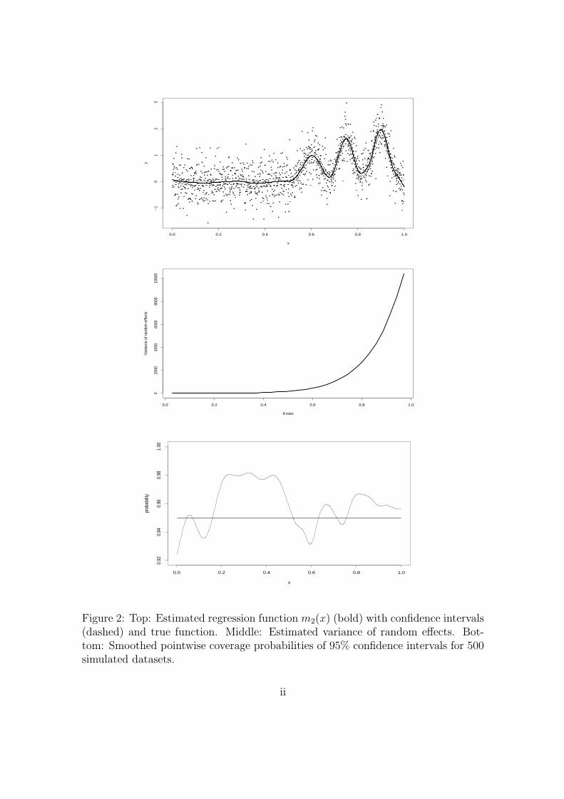
For comparison with Crainiceanu, Ruppert, Carroll, Adarsh & Goodner (2006) and
Lang & Brezger (2004) we consider the following regression function with moderate
spatial variability
m3(x1, x2) = x1 sin(4πx2),
with x1 and x2 independent and uniformly distributed on [0, 1]. We used n = 300,
σ = 1/4range(m3) and equally-spaced 12× 12 and 5× 5 knot grids for τ(b)i and τ
(c)j ,
respectively, as suggested by Crainiceanu, Ruppert, Carroll, Adarsh & Goodner
(2006). Figure 3 displays the true function (top left plot) and the resulting fit
for one simulation using our approach (top right plot) together with the estimated
variance of random effects (left bottom plot). We simulated 500 datasets to compare
14
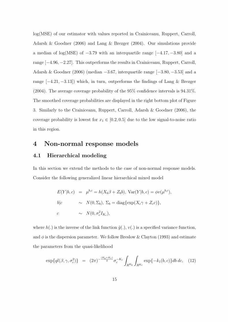
log(MSE) of our estimator with values reported in Crainiceanu, Ruppert, Carroll,
Adarsh & Goodner (2006) and Lang & Brezger (2004). Our simulations provide
a median of log(MSE) of −3.79 with an interquartile range [−4.17,−3.80] and a
range [−4.96,−2.27]. This outperforms the results in Crainiceanu, Ruppert, Carroll,
Adarsh & Goodner (2006) (median −3.67, interquartile range [−3.80,−3.53] and a
range [−4.21,−3.13]) which, in turn, outperforms the findings of Lang & Brezger
(2004). The average coverage probability of the 95% confidence intervals is 94.31%.
The smoothed coverage probabilities are displayed in the right bottom plot of Figure
3. Similarly to the Crainiceanu, Ruppert, Carroll, Adarsh & Goodner (2006), the
coverage probability is lowest for x1 ∈ [0.2, 0.5] due to the low signal-to-noise ratio
in this region.
4 Non-normal response models
4.1 Hierarchical modeling
In this section we extend the methods to the case of non-normal response models.
Consider the following generalized linear hierarchical mixed model
E(Y |b, c) = µb,c = h(Xbβ + Zbb), Var(Y |b, c) = φv(µb,c),
b|c ∼ N(0, Σb), Σb = diagexp(Xcγ + Zcc),
c ∼ N(0, σ2cIKc),
where h(.) is the inverse of the link function g(.), v(.) is a specified variance function,
and φ is the dispersion parameter. We follow Breslow & Clayton (1993) and estimate
the parameters from the quasi-likelihood
expql(β, γ, σ2c ) = (2π)−
(Kb+Kc)
2 σ−Kcc
∫
RKb
∫
RKc
exp−k1(b, c)db dc, (12)
15
where
k1(b, c) =1
2φ
∑qi(yi, µ
b,ci ) +
1
2bT Σ−1
b b +1
2log |Σb|+ 1
2σ2c
cT c,
and qi(y, µ) = −2∫ µ
y(y − t)/v(t)dt is the deviance function. Assuming that condi-
tionally on b and c the observations are drawn from the exponential family Y |b, c ∼exp([yϑ(x)− bϑ(x)]/φ + c(y, φ)), the quasi-likelihood (12) is the likelihood of the
data. Using Laplace’s method for approximation of the integral over b one obtains
expql(β, γ, σ2c ) ≈ (2π)−
Kc2 σ−Kc
c
∫
RKc
exp−k2(c)dc, (13)
where
k2(c) =1
2log |In + ZT
b WZbΣb|+ 1
2φ
∑qi(yi, µ
b,ci ) +
1
2bT Σ−1
b b +1
2σ2c
cT c,
b is the solution to
∂k1(b, c)
∂b= −ZT
b Wdiagg′(µb,c)(Y − µb,c) + Σ−1b b = 0.
Here W denotes the n×n diagonal matrix of the GLM iterated weights with diagonal
elements wi = [φv(µb,ci )g′(µb,c
i )2]−1, using the simplifying assumption that the
iterative weights wi vary slowly as a function of the mean.
Substituting the current estimate b into (13) and replacing the deviance∑
qi(yi, µb,ci )
in k2(.) by the Pearson chi-squared statistic∑
(yi − µb,ci )2/vi(µ
b,ci ) provides the fol-
lowing approximation
expql(β, γ, σ2c ) ≈ (2π)−
Kc2 σ−Kc
c |W |−1/2
∫
RKc
exp−k3(c)dc,
where k3(c) = 12log |V |+ cT c
2σ2c+(U −Xbβ)T V −1(U −Xbβ), V = W−1 +ZbΣbZ
Tb , and
U = Xbβ + Zbb + diagg′(µb,c)(Y −µb,c). Applying again Laplace’s method we end
up with the following quasi-log-likelihood for the remaining parameters
−2l(β, γ, σ2c ) ≈ Kc log σ2
c + log |V |+ log |kcc3 |
+ cT c/σ2c + (U −Xbβ)T V −1(U −Xbβ),
16
where kcc3 = ∂2k3(c)/∂c∂cT . As in Section 2 the estimation of parameter θ =
(γT , cT )T can be carried out from the score equation
∂k3(θ)
∂θ= −1
2W T
c Σ−1b
(b2 − wdfσ
2b
)+ Dcθ/σ
2c = 0. (14)
As in the normal case, the algorithm iterates between estimation of θ and generalized
linear mixed models fitting implemented in standard software.
4.2 Simulations for non-normal response models
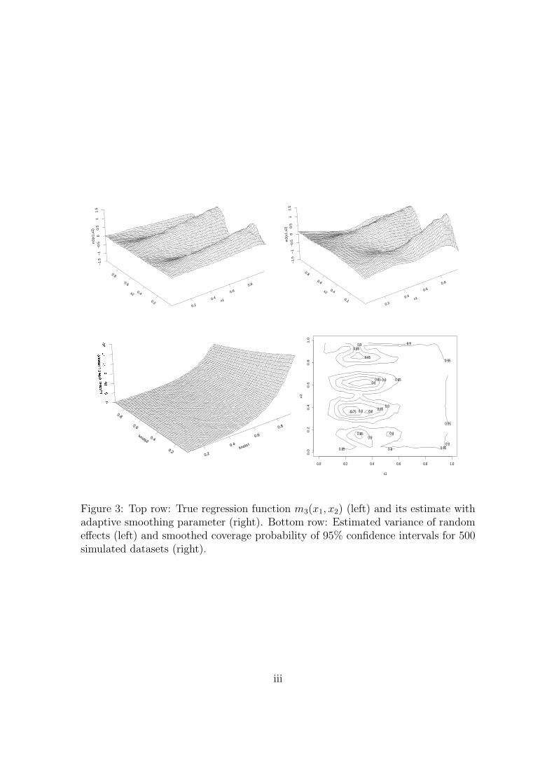
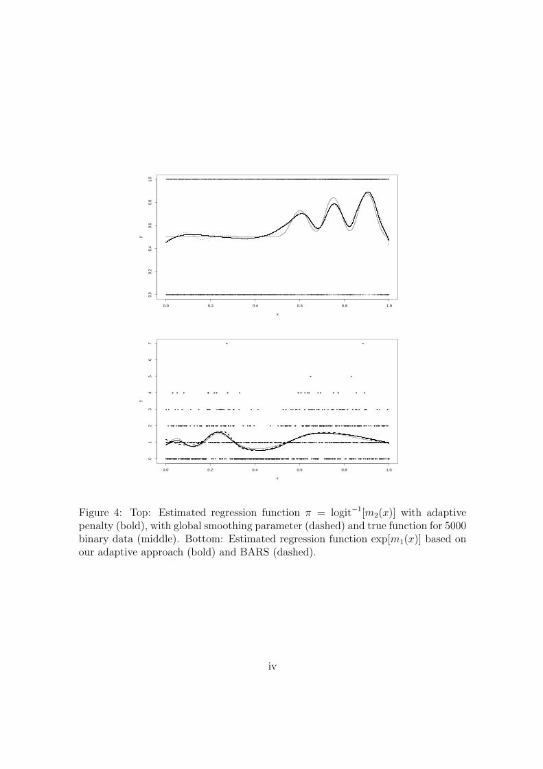
We consider the following model for Bernoulli data Yi ∼ B(1, πi) with canonical
link logit(πi) = m2(xi) where m2(.) is the function introduced in Section 2. The
top plot of Figure 4 represents the adaptive fit (bold line) for a data set of size
n = 5000. For comparison the non-adaptive fit (dashed line) is also shown indicating
the superiority of the adaptive fit. While the benefits of adaptive fit with binary
data are more clearly visible for large sample sizes, the adaptive procedure does not
require very large sample sizes to provide functional estimates. Depending on the
sample size and signal-to-noise ratio the adaptive fit would produce fits that are
closer or further away from its non-adaptive counterpart.
Since the method in this paper is the first one that can provide adaptive smoothing
for binary data, we cannot compare our method to others. However, the BARS
procedure of DiMatteo, Genovese & Kass (2001) allows fitting Poisson responses.
We performed a number of simulations to compare the performance of our routine
with the BARS implemented for this setting. We simulated n = 800 Poisson variates
with means expm1(x), where m1(.) was introduced in Section 2.5, and use j = 4
which corresponds to moderate heterogeneity. We estimated the data with our
approach using Kb = 60 and Kc = 10 and with the BARS procedure. We ran
10000 MCMC iterations with a burn-in sample of 2000. The bottom plot of Figure
17

4 displays estimates based on our adaptive approach (bold) and BARS (dashed).
The AMSE of the five fits based on our approach is 0.010672, while the AMSE
for BARS based fits is 0.020547. We did not perform a more extensive simulation
study, since a single BARS fit required more than 4 hours estimation time on an
up-to-date computer. For comparison, our function asp required only one minute.
We experimented with other mean functions and sample sizes and obtained very
similar results.
4.3 Example
As an illustration we apply spatially adaptive smoothing methods to a dataset on
the absenteeism of workers at a company in Germany. Parts of the data have been
analyzed before in Kauermann & Ortlieb (2004) with a different focus. We consider
absenteeism spells and model the probability of returning to work after a sick leave.
Denoting the duration of such a leave by d, we model the discrete hazard rate as
P (d = t|d ≥ t) = h(t), where t ≥ 1. The duration is measured in days and the
event of interest is ”recovery”, which allows workers to return to work. If the worker
reported sick on one day but returns to work on a consecutive working day thereafter,
we count this as an event and the duration is the number of working days the worker
had been absent. If the last day of absenteeism and the first day of returning to
work are not consecutive working days the duration is viewed as censored with d
being the number of days of absenteeism. To make this more explicit, assume that
a worker reports sick on Friday but returns to work the Monday after. It is unclear
when the worker actually recovered, either Friday, Saturday or Sunday. It is however
known, that the worker was at least sick on one day and the observation is therefore
d = 1 with censoring being indicated. Let δ denote the censoring indicator, which
18
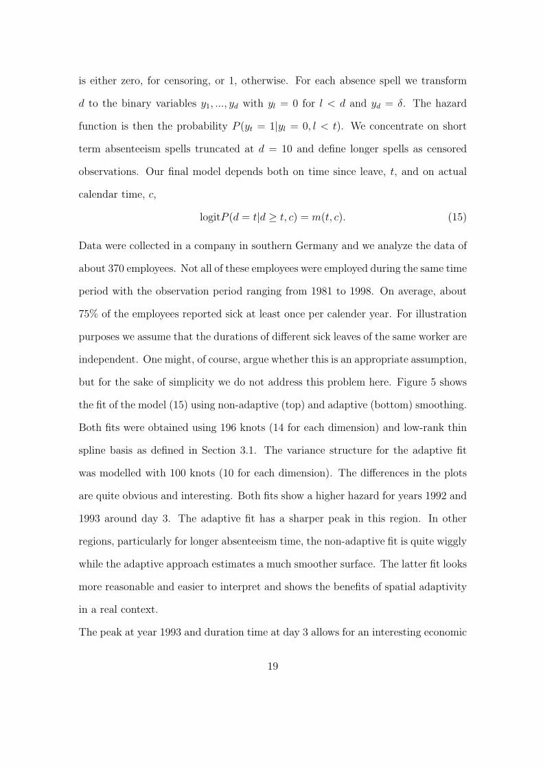
is either zero, for censoring, or 1, otherwise. For each absence spell we transform
d to the binary variables y1, ..., yd with yl = 0 for l < d and yd = δ. The hazard
function is then the probability P (yt = 1|yl = 0, l < t). We concentrate on short
term absenteeism spells truncated at d = 10 and define longer spells as censored
observations. Our final model depends both on time since leave, t, and on actual
calendar time, c,
logitP (d = t|d ≥ t, c) = m(t, c). (15)
Data were collected in a company in southern Germany and we analyze the data of
about 370 employees. Not all of these employees were employed during the same time
period with the observation period ranging from 1981 to 1998. On average, about
75% of the employees reported sick at least once per calender year. For illustration
purposes we assume that the durations of different sick leaves of the same worker are
independent. One might, of course, argue whether this is an appropriate assumption,
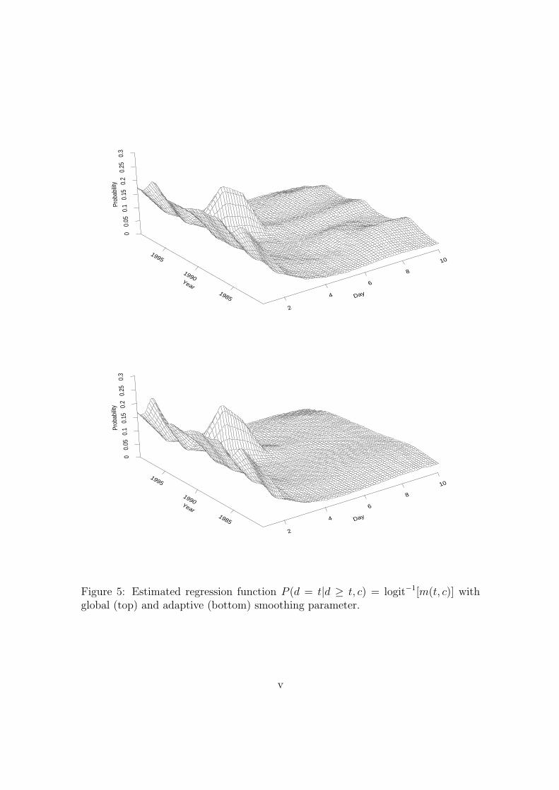
but for the sake of simplicity we do not address this problem here. Figure 5 shows
the fit of the model (15) using non-adaptive (top) and adaptive (bottom) smoothing.
Both fits were obtained using 196 knots (14 for each dimension) and low-rank thin
spline basis as defined in Section 3.1. The variance structure for the adaptive fit
was modelled with 100 knots (10 for each dimension). The differences in the plots
are quite obvious and interesting. Both fits show a higher hazard for years 1992 and
1993 around day 3. The adaptive fit has a sharper peak in this region. In other
regions, particularly for longer absenteeism time, the non-adaptive fit is quite wiggly
while the adaptive approach estimates a much smoother surface. The latter fit looks
more reasonable and easier to interpret and shows the benefits of spatial adaptivity
in a real context.
The peak at year 1993 and duration time at day 3 allows for an interesting economic
19
interpretation. In 1992/93 the company went through a major downsizing process
with more than 50% of the workers being dismissed. While this economic situation
has hardly any effect on the hazard function for days d ≥ 5, it does affect the hazard
rate for short absenteeism times, particularly for d = 3. According to the German
law, workers who report sick for more than 3 consecutive working days have to
provide a medical certificate at the latest at the third day of their sick leave. For
shorter periods no special attestation is required. Apparently, during the downsizing
period the duration of sick leaves is shorter with more employees returning after 3
days. This provides indication that economically critical conditions of a company
have a direct influence on the absenteeism of employees.
5 Conclusion
We showed that local adaptive smoothing can be easily carried out by formulating
penalties on the spline coefficient as a hierarchical mixed model. Our major contri-
bution was to show that the Laplace approximation of the marginal likelihood allows
fast fitting of adaptive smoothing models with application to univariate, bivariate
smoothing as well as to non-normal responses. For reasonably sized data sets and
normal responses our algorithm requires seconds while Bayesian MCMC simulations
require tens of minutes. For non-normal responses our algorithm requires less than a
minute while Bayesian MCMC requires more than several hours. In addition, small
changes to the model, such as adding a covariate, standard random effects, or other
smooth components, can be handled very easily by our methods, whereas it may
take hours, days, or even weeks for developing new MCMC software. An impor-
tant reason for having a fast and accurate procedure is that in many situations the
smoothing procedure needs to be applied repeatedly. One trivial example is when
20
doing simulations (note, for example how long it would take to perform the BARS
simulations in Section 4.2).
A R Package “AdaptFit”
To implement our approach we developed an R package. We took advantage of the R
package “SemiPar”, written by M.P. Wand to accompany the book Ruppert, Wand
& Carroll (2003). The function spm of this package performs scatterplot, spatial and
generalized (binomial and poisson) smoothing using the (generalized) mixed models
representation of penalized splines. This function handles additive models as well.
To perform adaptive smoothing we had to integrate the Fisher scoring procedure (9)
for θ with updates of the remaining parameters by subsequent calls of function spm.
The current version of our package “AdaptFit” with the function asp is available at
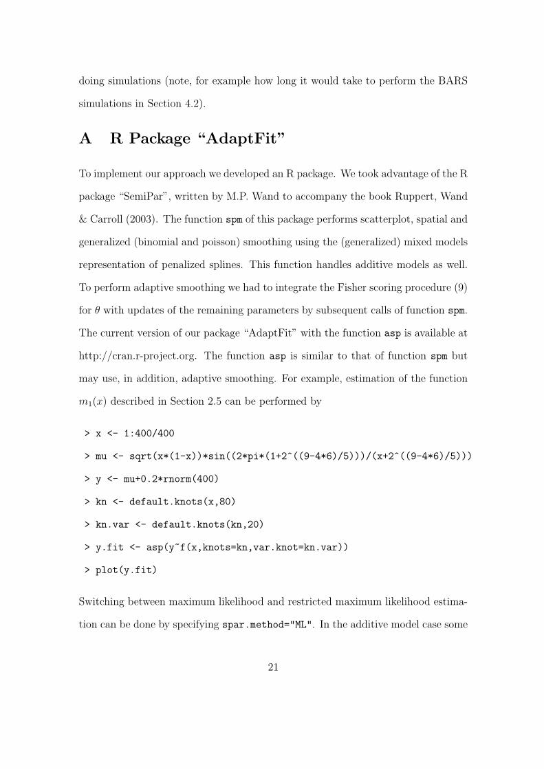
http://cran.r-project.org. The function asp is similar to that of function spm but
may use, in addition, adaptive smoothing. For example, estimation of the function
m1(x) described in Section 2.5 can be performed by
> x <- 1:400/400
> mu <- sqrt(x*(1-x))*sin((2*pi*(1+2^((9-4*6)/5)))/(x+2^((9-4*6)/5)))
> y <- mu+0.2*rnorm(400)
> kn <- default.knots(x,80)
> kn.var <- default.knots(kn,20)
> y.fit <- asp(y~f(x,knots=kn,var.knot=kn.var))
> plot(y.fit)
Switching between maximum likelihood and restricted maximum likelihood estima-
tion can be done by specifying spar.method="ML". In the additive model case some
21

components of the model can be fitted non-adaptively. Other examples are provided
within the package.
Acknowledgements
The work was conducted while the first author was affiliated to the University Biele-
feld. She wishes to thank for a productive working environment. The fist and third
author are also indebted to the Deutsche Forschungsgemeinschaft (DFG) for partial
support.
22
References
Baladandayuthapani, V., Mallick, B., and Carroll, R. (2005). Spatially adaptive
Bayesian penalized regression splines (P-splines). Journal of Computaional
and Graphical Statistics 14, 378–394.
Breslow, N. E. and Clayton, D. G. (1993). Approximate inference in generalized
linear mixed model. Journal of the American Statistical Association. 88, 9–25.
Crainiceanu, C., Ruppert, D., Carroll, R., Adarsh, J., and Goodner, B. (2006).
Spatially adaptive Bayesian P-splines with heteroscedastic errors. Journal of
Computational and Graphical Statistics , (to appear).
Crainiceanu, C., Ruppert, D., and Wand, M. (2005). Bayesian analysis for penal-
ized spline regression using WinBUGS. Journal of statistical software 14(14).
DiMatteo, I., Genovese, R., and Kass, R. (2001). Bayesian curve-fitting with free-
knots splines. Biometrika 88, 1055–1071.
Eilers, P. H. C. and Marx, B. D. (1996). Flexible smoothing with B-splines and
penalties. Stat. Science 11 (2), 89–121.
Fan, J. and Gijbels, I. (1995). Data-driven bandwidth selection in local polyno-
mial fitting: Variable bandwidth and spatial adaptation. Journal of the Royal
Statistical Society, Series B 57, 371–394.
Friedman, J. H. and Silverman, B. W. (1989). Flexible parsimonious smoothing
and additive modelling. Technometrics 31, 3–39.
Harville, D. (1977). Maximum likelihood approaches to variance component esti-
mation and to related problems. Journal of the American Statistical Associa-
tion. 72, 320–338.
23
Herrmann, E. (1997). Local bandwidth choice in kernel regression estimation.
Journal of Computational and Graphical Statistics 6, 35–54.
Kass, R. and Steffey, D. (1989). Approximate Bayesian inference in condition-
ally independent hierarchical models (parametric empirical Bayesian models).
Journal of the American Statistical Association. 84, 717–726.
Kauermann, G. (2004). A note on smoothing parameter selection for penalized
spline smoothing. Journal of Statistical Planing and Inference 127, 53–69.
Kauermann, G. and Ortlieb, R. (2004). Temporal pattern in the number of staff
on sick leave: the effect of downsizing. Journal of the Royal Statistical Society,
Series C 53, 353–367.
Kaufman, L. and Rousseeuw, P. (1990). Finding Groups in Data: An Introduction
to Cluster Analysis. New York: Wiley.
Laird, N. and Louis, T. (1987). Empirical Bayes confidence intervals based on
bootstrap samples (with discussion). Journal of the American Statistical As-
sociation. 82, 739–757.
Lang, S. and Brezger, A. (2004). Bayesian P-splines. Journal of Computational
and Graphical Statistics 13, 183–212.
Luo, Z. and Wahba, G. (1997). Hybrid adaptive splines. Journal of the American
Statistical Association 92, 107–116.
Morris, C. (1983). Parametric empirical Bayes inference: theory and applications
(with discussion). Journal of the American Statistical Association. 78, 47–65.
Ngo, L. and Wand, M. (2004). Smoothing with mixed model software. Journal of
statistical software 9(1).
24
O’Sullivan, F. (1986). A statistical perspective on ill-posed inverse problems (c/r:
P519-527). Statistical Science 1, 502–518.
Pintore, A., Speckman, P., and Holmes, C. C. (2005). Spatially adaptive smooth-
ing splines. Biometrika, (to appear).
Ruppert, D. (2002). Selecting the number of knots for penalized splines. Journal
of Computational and Graphical Statistics 11, 735–757.
Ruppert, D. and Carroll, R. (2000). Spatially-adaptive penalties for spline fitting.
Australian and New Zealand Journal of Statistics 42, 205–224.
Ruppert, R., Wand, M., and Carroll, R. (2003). Semiparametric Regression. Cam-
bridge University Press.
Searle, S., Casella, G., , and McCulloch, C. (1992). Variance Components. Wiley.
Severini, T. A. (2000). Likelihood Methods in Statistics. Oxford: Oxford University
Press.
Wand, M. (2003). Smoothing and mixed models. Computational Statistics 18,
223–249.
Wood, S., Jiang, W., and Tanner, M. (2002). Bayesian mixture of splines for
spatially adaptive nonparametric regression. Biometrika 89, 513–528.
25
0.0 0.2 0.4 0.6 0.8 1.0
−0.5
0.0
0.5
x
y
0.0 0.2 0.4 0.6 0.8 1.0
050
0010
000
1500
020
000
2500
030
000
3500
0
Knots
Var
ianc
e of
rand
om e
ffect
s
x
prob
abilit
y
0.0 0.2 0.4 0.6 0.8 1.0
0.70
0.75
0.80
0.85
0.90
0.95
1.00
Figure 1: Top: Estimated regression function m1(x) (bold) with confidence intervals(dashed) and true function. Middle: Estimated variance of random effects. Bot-tom: Smoothed pointwise coverage probabilities of 95% confidence intervals for 500simulated datasets.
i
0.0 0.2 0.4 0.6 0.8 1.0
−10
12
3
x
y
0.0 0.2 0.4 0.6 0.8 1.0
020
0040
0060
0080
0010
000
Knots
Var
ianc
e of
rand
om e
ffect
s
x
prob
abilit
y
0.0 0.2 0.4 0.6 0.8 1.0
0.92
0.94
0.96
0.98
1.00
Figure 2: Top: Estimated regression function m2(x) (bold) with confidence intervals(dashed) and true function. Middle: Estimated variance of random effects. Bot-tom: Smoothed pointwise coverage probabilities of 95% confidence intervals for 500simulated datasets.
ii
0.2
0.4
0.6
0.8
x10.2
0.4
0.6
0.8
x2
−1.
5−
1−
0.5
00.
51
1.5
m3(
x1,x
2)
0.2
0.4
0.6
0.8
x10.2
0.4
0.6
0.8
x2−
1.5
−1
−0.
5 0
0.5
11.
5m
3(x1
,x2)
x1
x2
0.0 0.2 0.4 0.6 0.8 1.0
0.0
0.2
0.4
0.6
0.8
1.0
0.75 0.8
0.8
0.80.85
0.85
0.85
0.85
0.85
0.9
0.9
0.9
0.9
0.9
0.9
0.90.9
0.95
0.95
0.95 0.95
0.95
Figure 3: Top row: True regression function m3(x1, x2) (left) and its estimate withadaptive smoothing parameter (right). Bottom row: Estimated variance of randomeffects (left) and smoothed coverage probability of 95% confidence intervals for 500simulated datasets (right).
iii
0.0 0.2 0.4 0.6 0.8 1.0
0.0
0.2
0.4
0.6
0.8
1.0
x
y
0.0 0.2 0.4 0.6 0.8 1.0
01
23
45
67
x
y
Figure 4: Top: Estimated regression function π = logit−1[m2(x)] with adaptivepenalty (bold), with global smoothing parameter (dashed) and true function for 5000binary data (middle). Bottom: Estimated regression function exp[m1(x)] based onour adaptive approach (bold) and BARS (dashed).
iv
2
4
6
8
10
Day1985
1990
1995
Year
00.
050.
10.
150.
20.
250.
3Pr
obab
ility
2
4
6
8
10
Day1985
1990
1995
Year
00.
050.
10.
150.
20.
250.
3Pr
obab
ility
Figure 5: Estimated regression function P (d = t|d ≥ t, c) = logit−1[m(t, c)] withglobal (top) and adaptive (bottom) smoothing parameter.
v