Fast and automatic microseismic phase-arrival detection anddenoising by pattern recognition and reduced-rank filtering

Danilo Velis1, Juan I. Sabbione2, and Mauricio D. Sacchi2

ABSTRACT

We have developed a fast method that allowed us to automati-cally detect and denoise microseismic phase arrivals from 3Cmultichannel data. The method is a two-step process. First, thedetection is carried out by means of a pattern recognition strat-egy that seeks plausible hyperbolic phase arrivals immersed innoisy 3C multichannel data. Then, the microseismic phase arriv-als are denoised and reconstructed using a reduced-rank ap-proximation of the singular value decomposition of the dataalong the detected phase arrivals in the context of a deflationprocedure that took into account multiple arrivals and/or phases.For the detection, we have defined an objective function thatmeasured the energy and coherence of a potential microseismicphase arrival along an apex-shifted hyperbolic search window.

The objective function, which was maximized using very fastsimulated annealing, was based on the energy of the averagesignal and depended on the source position, receivers geometry,and velocity. In practice, the detection process did not requireany a priori velocity model, leading to a fast algorithm that canbe used in real time, even when the underlying velocity modelwas not constant. The reduced-rank filtering coupled with acrosscorrelation-based synchronization strategy allowed us toextract the most representative waveform for all the individualtraces. Tests using synthetic and field data have determined thereliability and effectiveness of the proposed method for the ac-curate detection and denoising of 3C multichannel microseismicevents under noisy conditions. Two confidence indicators to as-sess the presence of an actual phase arrival and the reliability ofthe denoised individual wave arrivals were also developed.

INTRODUCTION

The study of microseismic data has become an essential tool inmany geoscience fields, such as oil reservoir geophysics (Maxwellet al., 2010; Kendall et al., 2011), mining engineering (Sun et al.,2012), and CO2 sequestration (Zhou et al., 2010). In hydraulic frac-turing, microseismicity studies permit the characterization andmonitoring of the reservoir dynamics to optimize the productionand the fluid injection process itself. Often, real-time functionalityis needed to control the fluid injection in the field for economic andsafety reasons. Besides, because the number of events is usuallylarge and the signal-to-noise ratio (S/N) is generally very low (es-pecially when receivers are located at the surface), fast, automated,and robust detection algorithms are required for most applications(Zimmer and Jin, 2011). Furthermore, inadequate array coverage

and uncertainties in the P- and S-wave underlying velocity modelscomplicate the processing of the data (Eisner et al., 2010).A basic workflow includes processes such as denoising, detec-

tion, picking, and localization (van der Baan et al., 2013). Gener-ally, microseismic events are detected (and located) by means ofgrid-search algorithms (Maxwell, 2014). These techniques are veryeffective and accurate but computationally intensive when dealingwith large 3D or 4D grids (Lagos et al., 2014). Other methods re-quire picking before carrying out localization, and others are able tolocate the microseisms without any picking at all (Gharti et al.,2010). As for detection, some techniques are based on the analysisof the changes of a certain attribute along individual channels, suchas trace energy (Munro, 2004), its absolute value (Chen and Stew-art, 2006), or a combination of short time average over long timeaverage (STA/LTA) and the wavelet transform (Vera Rodriguez,

Manuscript received by the Editor 28 November 2014; revised manuscript received 14 May 2015; published online 27 July 2015.1Universidad Nacional de La Plata, Facultad de Ciencias Astronómicas y Geofísicas, La Plata, Argentina and CONICET, Argentina. E-mail:

velis@fcaglp.unlp.edu.ar.2University of Alberta, Department of Physics and Signal Analysis and Imaging Group, Edmonton, Alberta, Canada. E-mail: jsabbione@fcaglp.unlp.edu.ar;

msacchi@ualberta.ca.© 2015 Society of Exploration Geophysicists. All rights reserved.

WC25

GEOPHYSICS, VOL. 80, NO. 6 (NOVEMBER-DECEMBER 2015); P. WC25–WC38, 12 FIGS., 2 TABLES.10.1190/GEO2014-0561.1

Dow

nloa

ded

09/2

3/15

to 1

42.2

44.1

91.6

0. R

edis

trib

utio

n su

bjec

t to

SEG

lice

nse

or c

opyr

ight

; see

Ter

ms

of U

se a

t http

://lib

rary

.seg

.org

/

2011), to name a few. Nevertheless, any single-channel event de-tection algorithm is prone to fail at some point whenever the S/N is very poor because not all data information is taken into accountsimultaneously. Thus, the key of a reliable event-detection algo-rithm relies on its ability to incorporate all the multichannel infor-mation at once. Sabbione and Velis (2013) follow this strategy anddevise a simple method based on single-trace phase pickers bor-rowed from global seismology that uses all channels simultane-ously. Zimmer and Jin (2011) and Gharti et al. (2010), forexample, describe the so-called migration-based approach. This ap-proach uses the information contained in a kind of stack of the inputchannels and does not require any trace-by-trace preprocessing forpicking the individual arrivals. Likewise, Radon-based techniques(Sabbione et al., 2013, 2015) also rely on the information containedin all the channels simultaneously.In this work, we present a fast two-stage method that does not

require the knowledge of the underlying velocity model because aneffective constant velocity is obtained as a by-product. First, we ac-complish the detection by solving a pattern recognition problemvery efficiently using very fast simulated annealing (VFSA) (Veliset al., 2013). This leads to a fully automatic and reliable micro-seismic phase-arrival detection algorithm that includes a deflationprocess used to deal with multiple phases and/or arrivals and a con-fidence indicator to assess the significance of the detections. Sec-ond, we denoise and reconstruct the detected phase arrivals using asingular value decomposition (SVD)-based reduced-rank filteringapproach, which leads to consistent waveforms that preserve ampli-

tudes throughout all available channels and components. As weshow in the next sections, under certain assumptions, microseismicphase arrivals are characterized by coherent arrivals along hyper-bolic patterns. Then, imperfect alignments are tolerated by meansof a crosscorrelation-based synchronization process that is appliedbefore the filtering. In addition, we provide another confidence in-dicator to assess the significance of the reconstructed phase arrivalson a trace-by-trace basis. By means of examples, we show that theproposed technique behaves very effectively and accurately whenapplied to moderate to high-S/N synthetic and field data sets, andreasonably well when applied to very noisy data sets. Overall, thedetection is robust in the presence of random noise and isolatedtraces with useless information, the derived traveltimes are accurate,and the reconstructed waveforms are consistent with the observeddata, even when the underlying velocity model is unknown.

THEORY

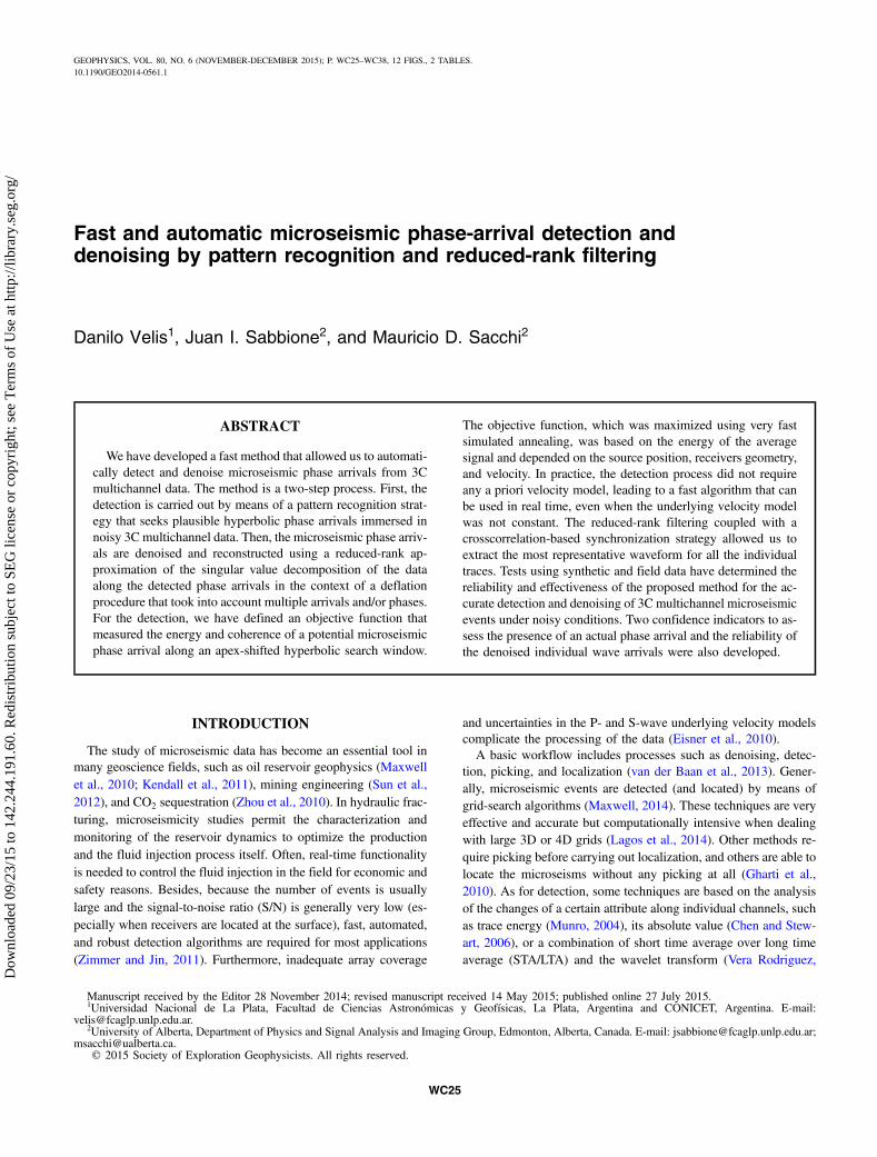
Consider a 2D typical downhole microseismic monitoring sce-nario as shown in Figure 1a. Assuming a constant velocity medium,the arrival time at the receiver ðx; zÞ due to a microseism originatedat ðxs; zsÞ can be expressed by

tðx; zÞ ¼ t0 þrðx; zÞ

v; (1)

where

rðx; zÞ ¼ffiffiffiffiffiffiffiffiffiffiffiffiffiffiffiffiffiffiffiffiffiffiffiffiffiffiffiffiffiffiffiffiffiffiffiffiffiffiffiffiffiðx − xsÞ2 þ ðz − zsÞ2

q(2)

is the source-receiver distance, v is the P- or S-wave velocity, and t0is the occurrence time of the event measured relatively to the starttime of the recorded seismic traces.

Cones and hyperbolas

Equation 1 can be rewritten as

ðx − xsÞ2v2

þ ðz − zsÞ2v2

¼ ðt − t0Þ2; (3)

which is the equation of a right circular cone in ðx; z; tÞ centered atðxs; zs; t0Þ. Figure 1b shows part of this quadratic surface forðxs; zsÞ ¼ ð0.5; 1.6Þ km, t0 ¼ 0 s, and v ¼ 2.4 km∕s. When a coneis sliced vertically, a hyperbola is obtained. For this reason, for a setof receivers placed along a straight monitoring well (vertical orslanted), as depicted in Figure 1a, the time arrivals align along anapex-shifted hyperbola (Figure 1b). Should the receiver array not bealigned along a straight line, a fact that depends on the local con-ditions of the monitoring well and the engineering objectives, thearrival times will no longer align along a hyperbola. Thus, for the sakeof generality, rather than assuming that the arrival times are alignedalong a hyperbola, one may assume that in fact they are placed on acone (or a hypercone in a 3D scenario). In practice, however, mostmonitoring wells are approximately straight along the extension ofthe receiver array; hence, the hyperbolic approximation is perfectlyvalid for constant velocity models. For nonconstant velocity models,raypaths are not straight lines. Thus, despite the fact that equation 1can be generalized by redefining rðx; zÞ∕v as the traveltime fromsource to receiver, arrivals are no longer expected to be aligned

1

1.2

1.4

1.6

1.8

2 0 0.1 0.2 0.3 0.4 0.5 0.6

R1

R8

Source

r

z (k

m)

x (km)

a)

b)

Monitoring well

0 0.2 0.4 0.6 0.8

1.2

1.6

2

0

0.1

0.2

0.3

R1R8

x (km)

z (km)

t(x,

z) (

s)t(

x,z)

(s)

Figure 1. (a) Typical 2D downhole microseismic monitoring sce-nario and (b) the cone represents the arrival times expressed in equa-tion 3. For a linear monitoring well, arrivals are aligned along anapex-shifted hyperbola. The R1 and R8 denote the first and eighthreceivers, respectively.

WC26 Velis et al.

Dow

nloa

ded

09/2

3/15

to 1

42.2

44.1

91.6

0. R

edis

trib

utio

n su

bjec

t to

SEG

lice

nse

or c

opyr

ight

; see

Ter

ms

of U

se a

t http

://lib

rary

.seg

.org

/

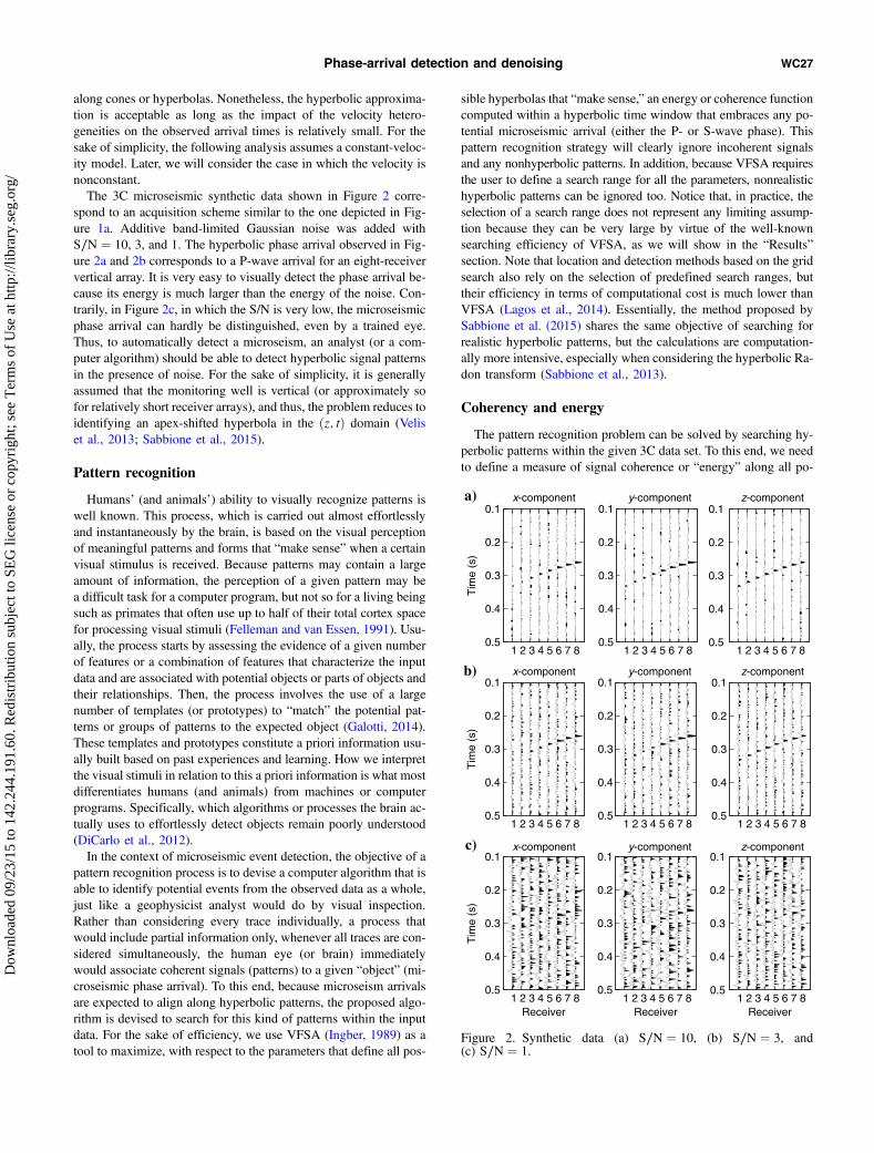
along cones or hyperbolas. Nonetheless, the hyperbolic approxima-tion is acceptable as long as the impact of the velocity hetero-geneities on the observed arrival times is relatively small. For thesake of simplicity, the following analysis assumes a constant-veloc-ity model. Later, we will consider the case in which the velocity isnonconstant.The 3C microseismic synthetic data shown in Figure 2 corre-

spond to an acquisition scheme similar to the one depicted in Fig-ure 1a. Additive band-limited Gaussian noise was added withS∕N ¼ 10, 3, and 1. The hyperbolic phase arrival observed in Fig-ure 2a and 2b corresponds to a P-wave arrival for an eight-receiververtical array. It is very easy to visually detect the phase arrival be-cause its energy is much larger than the energy of the noise. Con-trarily, in Figure 2c, in which the S/N is very low, the microseismicphase arrival can hardly be distinguished, even by a trained eye.Thus, to automatically detect a microseism, an analyst (or a com-puter algorithm) should be able to detect hyperbolic signal patternsin the presence of noise. For the sake of simplicity, it is generallyassumed that the monitoring well is vertical (or approximately sofor relatively short receiver arrays), and thus, the problem reduces toidentifying an apex-shifted hyperbola in the ðz; tÞ domain (Veliset al., 2013; Sabbione et al., 2015).

Pattern recognition

Humans’ (and animals’) ability to visually recognize patterns iswell known. This process, which is carried out almost effortlesslyand instantaneously by the brain, is based on the visual perceptionof meaningful patterns and forms that “make sense” when a certainvisual stimulus is received. Because patterns may contain a largeamount of information, the perception of a given pattern may bea difficult task for a computer program, but not so for a living beingsuch as primates that often use up to half of their total cortex spacefor processing visual stimuli (Felleman and van Essen, 1991). Usu-ally, the process starts by assessing the evidence of a given numberof features or a combination of features that characterize the inputdata and are associated with potential objects or parts of objects andtheir relationships. Then, the process involves the use of a largenumber of templates (or prototypes) to “match” the potential pat-terns or groups of patterns to the expected object (Galotti, 2014).These templates and prototypes constitute a priori information usu-ally built based on past experiences and learning. How we interpretthe visual stimuli in relation to this a priori information is what mostdifferentiates humans (and animals) from machines or computerprograms. Specifically, which algorithms or processes the brain ac-tually uses to effortlessly detect objects remain poorly understood(DiCarlo et al., 2012).In the context of microseismic event detection, the objective of a

pattern recognition process is to devise a computer algorithm that isable to identify potential events from the observed data as a whole,just like a geophysicist analyst would do by visual inspection.Rather than considering every trace individually, a process thatwould include partial information only, whenever all traces are con-sidered simultaneously, the human eye (or brain) immediatelywould associate coherent signals (patterns) to a given “object” (mi-croseismic phase arrival). To this end, because microseism arrivalsare expected to align along hyperbolic patterns, the proposed algo-rithm is devised to search for this kind of patterns within the inputdata. For the sake of efficiency, we use VFSA (Ingber, 1989) as atool to maximize, with respect to the parameters that define all pos-

sible hyperbolas that “make sense,” an energy or coherence functioncomputed within a hyperbolic time window that embraces any po-tential microseismic arrival (either the P- or S-wave phase). Thispattern recognition strategy will clearly ignore incoherent signalsand any nonhyperbolic patterns. In addition, because VFSA requiresthe user to define a search range for all the parameters, nonrealistichyperbolic patterns can be ignored too. Notice that, in practice, theselection of a search range does not represent any limiting assump-tion because they can be very large by virtue of the well-knownsearching efficiency of VFSA, as we will show in the “Results”section. Note that location and detection methods based on the gridsearch also rely on the selection of predefined search ranges, buttheir efficiency in terms of computational cost is much lower thanVFSA (Lagos et al., 2014). Essentially, the method proposed bySabbione et al. (2015) shares the same objective of searching forrealistic hyperbolic patterns, but the calculations are computation-ally more intensive, especially when considering the hyperbolic Ra-don transform (Sabbione et al., 2013).

Coherency and energy

The pattern recognition problem can be solved by searching hy-perbolic patterns within the given 3C data set. To this end, we needto define a measure of signal coherence or “energy” along all po-

0.1

0.2

0.3

0.4

0.5 1 2 3 4 5 6 7 8

Tim

e (s

)

x-componenta) 0.1

0.2

0.3

0.4

0.5 1 2 3 4 5 6 7 8

y-component 0.1

0.2

0.3

0.4

0.5 1 2 3 4 5 6 7 8

z-component

x-component y-component z-component

x-component y-component z-component

0.1

0.2

0.3

0.4

0.5 1 2 3 4 5 6 7 8

Tim

e (s

)

b) 0.1

0.2

0.3

0.4

0.5 1 2 3 4 5 6 7 8

0.1

0.2

0.3

0.4

0.5 1 2 3 4 5 6 7 8

0.1

0.2

0.3

0.4

0.5 1 2 3 4 5 6 7 8

Tim

e (s

)

Receiver

c) 0.1

0.2

0.3

0.4

0.5 1 2 3 4 5 6 7 8

Receiver

0.1

0.2

0.3

0.4

0.5 1 2 3 4 5 6 7 8

Receiver

Figure 2. Synthetic data (a) S∕N ¼ 10, (b) S∕N ¼ 3, and(c) S∕N ¼ 1.

Phase-arrival detection and denoising WC27

Dow

nloa

ded

09/2

3/15

to 1

42.2

44.1

91.6

0. R

edis

trib

utio

n su

bjec

t to

SEG

lice

nse

or c

opyr

ight

; see

Ter

ms

of U

se a

t http

://lib

rary

.seg

.org

/

tential hyperbolas (or cones), which are defined by ðxs; zs; t0; vÞ.Velis et al. (2013), for example, use the quantity

Genvðxs; zs; t0; vÞ ¼1

3M

XMi¼1

ðsxi þ syi þ szi Þ; (4)

where sci is the ith sample of the mean envelope (c ¼ x; y; z) alongthe trial hyperbola, and M is the number of samples (width) of thesearch window. Clearly, when Genv attains a maximum value, theprobability of having a phase arrival is high. Note that this measure,which is similar to those used by Michaud and Leaney (2008),Gharti et al. (2010), and Sabbione et al. (2015), is particularly verysensitive to the energy of the phase arrival, irrespective of any phasechanges.An alternative measure is the average energy of the mean traces:

Gseðxs; zs; t0; vÞ ¼1

3M

XMi¼1

½ðsxi Þ2 þ ðsyi Þ2 þ ðszi Þ2�; (5)

where sci is the ith sample of the normalized mean trace (c ¼ x; y; z)along the trial hyperbola of width M. This energy measure, whichwe call stack energy for simplicity, is similar to the semblance used in

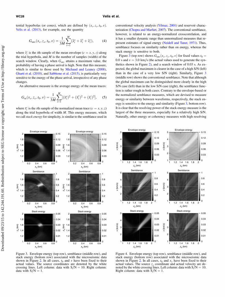
conventional velocity analysis (Yilmaz, 2001) and reservoir charac-terization (Chopra and Marfurt, 2007). The conventional semblance,however, is related to an energy-normalized crosscorrelation, andit has a smaller dynamic range than unnormalized measures that re-present estimates of signal energy (Neidell and Taner, 1971). Thus,semblance focuses on similarity rather than on energy, whereas thestack energy is sensitive to both.Figure 3 (top row) shows Genvðxs; zs; t0; vÞ for fixed values t0 ¼

0.0 s and v ¼ 3.0 km∕s (the actual values used to generate the syn-thetics shown in Figure 2), and a search window of 0.03 s. As ex-pected, the global maximum is clearer in the case of a high S/N (left)than in the case of a very low S/N (right). Similarly, Figure 3(middle row) shows the conventional semblance. Note that althoughthe global maximum can be distinguished more clearly in the highS/N case (left) than in the low S/N case (right), the semblance func-tion is rather rough in both cases. Contrary to the envelope-based orthe normalized semblance measures, which are devised to measureenergy or similarity between waveforms, respectively, the stack en-ergy is sensitive to the energy and similarity (Figure 3, bottom row).It is clear that the resolving power of the stack energy measure is thelargest of the three measures, especially for a relatively high S/N.Naturally, other energy or coherency measures with high resolving

Envelope energy

0.2 0.4 0.6 0.8xs (km)

1

1.2

1.4

1.6

1.8

2

z s (

km)

0

0.03

0.06

0.09

0.12

0.15Envelope energy

0.2 0.4 0.6 0.8xs (km)

1

1.2

1.4

1.6

1.8

2

z s (

km)

0

0.03

0.06

0.09

0.12

0.15

Semblance

0.2 0.4 0.6 0.8xs (km)

1

1.2

1.4

1.6

1.8

2

z s (

km)

0

0.2

0.4

0.6

0.8

1Semblance

0.2 0.4 0.6 0.8xs (km)

1

1.2

1.4

1.6

1.8

2

z s (

km)

0

0.2

0.4

0.6

0.8

1

Stack energy

0.2 0.4 0.6 0.8xs (km)

1

1.2

1.4

1.6

1.8

2

z s (

km)

0

0.01

0.02

0.03

0.04

0.05Stack energy

0.2 0.4 0.6 0.8xs (km)

1

1.2

1.4

1.6

1.8

2

z s (

km)

0

0.01

0.02

0.03

0.04

0.05

Figure 3. Envelope energy (top row), semblance (middle row), andstack energy (bottom row) associated with the microseismic datashown in Figure 2. In all cases, t0 and v have been fixed to theiractual values. The source coordinates are denoted by the whitecrossing lines. Left column: data with S∕N ¼ 10. Right column:data with S∕N ¼ 1.

Envelope energy

1 1.2 1.4 1.6 1.8 2zs (km)

1

2

3

4

5

v (k

m/s

)

0

0.03

0.06

0.09

0.12

0.15Envelope energy

1 1.2 1.4 1.6 1.8 2zs (km)

1

2

3

4

5

v (k

m/s

) 0

0.03

0.06

0.09

0.12

0.15

Semblance

1 1.2 1.4 1.6 1.8 2zs (km)

1

2

3

4

5

v (k

m/s

)

0

0.2

0.4

0.6

0.8

1Semblance

1 1.2 1.4 1.6 1.8 2zs (km)

1

2

3

4

5

v (k

m/s

)

0

0.2

0.4

0.6

0.8

1

Stack energy

1 1.2 1.4 1.6 1.8 2zs (km)

1

2

3

4

5

v (k

m/s

)

0

0.01

0.02

0.03

0.04

0.05Stack energy

1 1.2 1.4 1.6 1.8 2zs (km)

1

2

3

4

5

v (k

m/s

)

0

0.01

0.02

0.03

0.04

0.05

Figure 4. Envelope energy (top row), semblance (middle row), andstack energy (bottom row) associated with the microseismic datashown in Figure 2. In all cases, t0 and xs have been fixed to theiractual values. The source zs coordinate and actual velocity are de-noted by the white crossing lines. Left column: data with S∕N ¼ 10.Right column: data with S∕N ¼ 1.

WC28 Velis et al.

Dow

nloa

ded

09/2

3/15

to 1

42.2

44.1

91.6

0. R

edis

trib

utio

n su

bjec

t to

SEG

lice

nse

or c

opyr

ight

; see

Ter

ms

of U

se a

t http

://lib

rary

.seg

.org

/

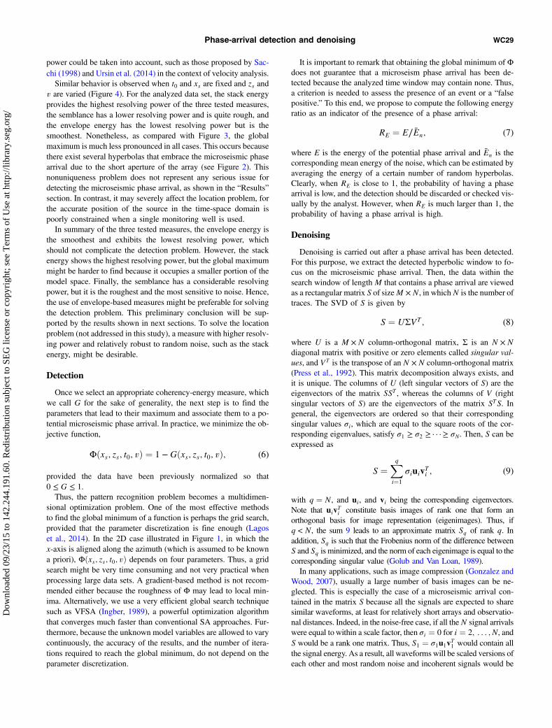
power could be taken into account, such as those proposed by Sac-chi (1998) and Ursin et al. (2014) in the context of velocity analysis.Similar behavior is observed when t0 and xs are fixed and zs and

v are varied (Figure 4). For the analyzed data set, the stack energyprovides the highest resolving power of the three tested measures,the semblance has a lower resolving power and is quite rough, andthe envelope energy has the lowest resolving power but is thesmoothest. Nonetheless, as compared with Figure 3, the globalmaximum is much less pronounced in all cases. This occurs becausethere exist several hyperbolas that embrace the microseismic phasearrival due to the short aperture of the array (see Figure 2). Thisnonuniqueness problem does not represent any serious issue fordetecting the microseismic phase arrival, as shown in the “Results”section. In contrast, it may severely affect the location problem, forthe accurate position of the source in the time-space domain ispoorly constrained when a single monitoring well is used.In summary of the three tested measures, the envelope energy is

the smoothest and exhibits the lowest resolving power, whichshould not complicate the detection problem. However, the stackenergy shows the highest resolving power, but the global maximummight be harder to find because it occupies a smaller portion of themodel space. Finally, the semblance has a considerable resolvingpower, but it is the roughest and the most sensitive to noise. Hence,the use of envelope-based measures might be preferable for solvingthe detection problem. This preliminary conclusion will be sup-ported by the results shown in next sections. To solve the locationproblem (not addressed in this study), a measure with higher resolv-ing power and relatively robust to random noise, such as the stackenergy, might be desirable.

Detection

Once we select an appropriate coherency-energy measure, whichwe call G for the sake of generality, the next step is to find theparameters that lead to their maximum and associate them to a po-tential microseismic phase arrival. In practice, we minimize the ob-jective function,

Φðxs; zs; t0; vÞ ¼ 1 − Gðxs; zs; t0; vÞ; (6)

provided the data have been previously normalized so that0 ≤ G ≤ 1.Thus, the pattern recognition problem becomes a multidimen-

sional optimization problem. One of the most effective methodsto find the global minimum of a function is perhaps the grid search,provided that the parameter discretization is fine enough (Lagoset al., 2014). In the 2D case illustrated in Figure 1, in which thex-axis is aligned along the azimuth (which is assumed to be knowna priori), Φðxs; zs; t0; vÞ depends on four parameters. Thus, a gridsearch might be very time consuming and not very practical whenprocessing large data sets. A gradient-based method is not recom-mended either because the roughness of Φ may lead to local min-ima. Alternatively, we use a very efficient global search techniquesuch as VFSA (Ingber, 1989), a powerful optimization algorithmthat converges much faster than conventional SA approaches. Fur-thermore, because the unknown model variables are allowed to varycontinuously, the accuracy of the results, and the number of itera-tions required to reach the global minimum, do not depend on theparameter discretization.

It is important to remark that obtaining the global minimum of Φdoes not guarantee that a microseism phase arrival has been de-tected because the analyzed time window may contain none. Thus,a criterion is needed to assess the presence of an event or a “falsepositive.” To this end, we propose to compute the following energyratio as an indicator of the presence of a phase arrival:

RE ¼ E∕En; (7)

where E is the energy of the potential phase arrival and En is thecorresponding mean energy of the noise, which can be estimated byaveraging the energy of a certain number of random hyperbolas.Clearly, when RE is close to 1, the probability of having a phasearrival is low, and the detection should be discarded or checked vis-ually by the analyst. However, when RE is much larger than 1, theprobability of having a phase arrival is high.

Denoising

Denoising is carried out after a phase arrival has been detected.For this purpose, we extract the detected hyperbolic window to fo-cus on the microseismic phase arrival. Then, the data within thesearch window of length M that contains a phase arrival are viewedas a rectangular matrix S of sizeM × N, in whichN is the number oftraces. The SVD of S is given by

S ¼ UΣVT; (8)

where U is a M × N column-orthogonal matrix, Σ is an N × Ndiagonal matrix with positive or zero elements called singular val-ues, and VT is the transpose of an N × N column-orthogonal matrix(Press et al., 1992). This matrix decomposition always exists, andit is unique. The columns of U (left singular vectors of S) are theeigenvectors of the matrix SST , whereas the columns of V (rightsingular vectors of S) are the eigenvectors of the matrix STS. Ingeneral, the eigenvectors are ordered so that their correspondingsingular values σi, which are equal to the square roots of the cor-responding eigenvalues, satisfy σ1 ≥ σ2 ≥ · · ·≥ σN. Then, S can beexpressed as

S ¼Xqi¼1

σiuivTi ; (9)

with q ¼ N, and ui, and vi being the corresponding eigenvectors.Note that uivTi constitute basis images of rank one that form anorthogonal basis for image representation (eigenimages). Thus, ifq < N, the sum 9 leads to an approximate matrix Sq of rank q. Inaddition, Sq is such that the Frobenius norm of the difference betweenS and Sq is minimized, and the norm of each eigenimage is equal to thecorresponding singular value (Golub and Van Loan, 1989).In many applications, such as image compression (Gonzalez and

Wood, 2007), usually a large number of basis images can be ne-glected. This is especially the case of a microseismic arrival con-tained in the matrix S because all the signals are expected to sharesimilar waveforms, at least for relatively short arrays and observatio-nal distances. Indeed, in the noise-free case, if all theN signal arrivalswere equal to within a scale factor, then σi ¼ 0 for i ¼ 2; : : : ; N, andS would be a rank one matrix. Thus, S1 ¼ σ1u1vT1 would contain allthe signal energy. As a result, all waveforms will be scaled versions ofeach other and most random noise and incoherent signals would be

Phase-arrival detection and denoising WC29

Dow

nloa

ded

09/2

3/15

to 1

42.2

44.1

91.6

0. R

edis

trib

utio

n su

bjec

t to

SEG

lice

nse

or c

opyr

ight

; see

Ter

ms

of U

se a

t http

://lib

rary

.seg

.org

/

attenuated, as we will show in the “Results” section. When wave-forms vary, the level of noise attenuation and waveform “homogeni-zation” can be controlled by the number of singular values used in theapproximation because the signal energy would be contained in thefirst (and largest) eigenimages.

Synchronization

Until now, we have assumed that the underlying velocity modelwas constant. This assumption has allowed us to describe the micro-seismic time arrivals by cones and/or hyperbolas. Clearly, when thevelocity model is heterogeneous, the signals are not expected toalign in such a geometrically simple way and a single parameterv used to fit the arrivals as in equation 3 is questionable. In spiteof this, as shown by Blias and Grechka (2013), a homogeneousmedium with an effective constant velocity may provide suitableconstraints to solve the microseismic event location problem andconstitute a simple and effective strategy to fit the arrival timesacceptably well in most scenarios. Naturally, the accuracy of theestimated hypocenters degrades with velocity heterogeneity. Insolving the detection problem, however, the constant velocityassumption is less restrictive because the velocity is only used indefining the search window. In this sense, it is enough that it con-tains the microseismic phase arrival, but it is not necessary that italigns very accurately along the actual hyperbolic phase arrival. It isemphasized that, as pointed out by Blias and Grechka (2013), thiseffective velocity represents a fitting parameter in the same way asthe stacking velocity is a fitting parameter in conventional velocityanalysis of seismic reflection data. Therefore, an estimate of theactual velocity model is not required for it will be obtained as aby-product when equation 6 is minimized.Nevertheless, the proposed method is general enough so as to

accommodate heterogeneous models whenever these models areavailable a priori. In fact, the energy or coherence measure is com-puted along a time-varying window, which may or may not follow asimple geometric curve or surface, depending on the velocity usedin equation 1. For nonconstant velocities, arrival time t, which de-fines the time-varying window, can be computed using either raytracing or any other technique for every tested triplet ðxs; zs; t0Þ,instead of ðxs; zs; t0; vÞ, at each SA iteration. Thus, although it iscomputationally more demanding, the number of unknowns is re-duced by one and the optimization of the corresponding cost func-tion should not be a problem provided the input velocity model isaccurate enough. Actually, most event location methods require theuser to provide an adequate velocity model. This velocity model,which is usually derived from sonic logs, should be properly cali-brated before proceeding to estimate the hypocenters (Maxwell,2014).Here, we provide an alternative strategy to allow for hetero-

geneous velocity models when these are not available. The useful-ness of this strategy relies on the assumption that the homogeneousvelocity approximation is good enough so as to provide a hyperbolathat embraces the potential phase arrival, whether the individualarrivals at each receiver are aligned or not. Then, the individual de-tected arrivals are synchronized by adding appropriate time shifts.By this means, it is possible to account for possible deviations be-tween the modeled and observed arrival times due to the velocitymodel assumption. This is a very important process for the denois-ing stage because SVD filtering assumes that the arrivals are alignedalong the final search window. Thus, once the phase arrival has been

detected in the framework of the constant velocity model assump-tion, we proceed to compute the average trace envelope within thefinal search window and time shift every individual arrival so as tomaximize the crosscorrelation between the average envelope andthe corresponding individual envelopes. This simple crosscorrela-tion-based synchronization process guarantees that all arrivals areproperly aligned before carrying out the denoising using theSVD. Finally, the time-shift corrections are undone to obtain thecorresponding denoised microseismic phase arrival. The describedstrategy is specially suited for relatively short arrays and when theimpact of the velocity heterogeneities on the time shifts are rela-tively small. Nevertheless, the strategy can also be applied when thevelocity model is available. In this case, the synchronization processcould account for possible deviations between the modeled andobserved phase-arrival times due to the uncertainties in the velocitymodel.

Deflation

Another assumption that we have used so far is that there is asingle phase arrival within the analyzed time window. However,data may contain P- and S-wave arrivals associated with one ormore microseismic events. Rather than detecting and denoising allsignal arrivals simultaneously, we propose to carry out the detectionand denoising of each individual signal arrival separately by meansof a deflation procedure. In this sense, once a phase arrival has beendetected and denoised using the described methods, the resultingdata are subtracted from the original data, leading to a residual dataset containing any other phase arrival that may have not been de-tected, denoised, and removed yet. Then, the residual is treated as anew data set for the detection and denoising. This deflation processis repeated until no new phase arrivals are detected (e.g., until RE issmaller than a given threshold value). Note that because the detec-tion process involves the minimization of the cost function 6 bymeans of SA, which is equivalent to locate the most energeticand/or coherent hyperbolic phase arrival within the analyzed timewindow, the deflation procedure implies that the most significantphase arrivals will be detected first. At the end of the deflation proc-ess, the residual is expected to contain noise only.The described deflation process resembles the well-known match-

ing pursuit algorithm, in which seismic traces are decomposed into aseries of “atoms” of decreasing energy selected from a large and re-dundant dictionary of basis functions (Mallat and Zhang, 1993). Usu-ally, dictionaries are built based on adaptive time-frequency wavelets(e.g., Gabor or Morlet wavelets) so that the time-varying signalstructure can be correctly represented by a relatively small numberof atoms (Liu and Marfurt, 2005; Wang, 2010). In the proposeddeflation process, instead of using predefined basis functions orwavelets, the microseismic signals are represented by a reduced-rank approximation of the SVD of the detected phase arrivals alonghyperbolic windows.

RESULTS

Synthetic example 1

First, we test the method using the 3C microseismic syntheticdata shown in Figure 2. These data sets contain a single microseis-mic phase arrival and correspond to a constant velocity model.Thus, cost function 6 is dominated by a single global minimum

WC30 Velis et al.

Dow

nloa

ded

09/2

3/15

to 1

42.2

44.1

91.6

0. R

edis

trib

utio

n su

bjec

t to

SEG

lice

nse

or c

opyr

ight

; see

Ter

ms

of U

se a

t http

://lib

rary

.seg

.org

/

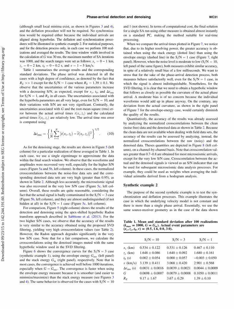
(although small local minima exist, as shown in Figures 3 and 4),and the deflation procedure will not be required. No synchroniza-tion would be required either because the individual arrivals arealigned along hyperbolas. The deflation and synchronization proce-dures will be illustrated in synthetic example 2. For statistical purposes,and for the detection process only, in each case we perform 100 real-izations and averaged the results. The time window width involved inthe calculation ofG was 30 ms, the maximum number of SA iterationswas 1000, and the search ranges were set as follows: xs ¼ 0 − 1 km,zs ¼ 0 − 2 km, t0 ¼ 0 − 0.2 s, and v ¼ 1 − 5 km∕s.Table 1 summarizes the average results and the corresponding

standard deviations. The phase arrival was detected in all thecases with a high degree of confidence, as denoted by the fact thatRE >> 1 except for the S∕N ¼ 1 case where RE ¼ 1.39� 0.1. Weobserve that the uncertainties of the various parameters increasewith a decreasing S/N, as expected, except for xs, t0, and Δtrms

for S∕N ¼ 1, and RE in all cases. The uncertainties associated withthe hyperbola parameters are all very large, even for S∕N ¼ 10, andtheir variations with S/N are not very significant. Contrarily, theuncertainties associated with G and the root-mean-square (rms) er-ror between the actual arrival times tðxi; ziÞ and the calculatedarrival times tðxi; ziÞ are relatively low. The arrival time rms erroris computed using

Δtrms ¼�1

N

XNi¼1

½tðxi; ziÞ − tðxi; ziÞ�2�1∕2

: (10)

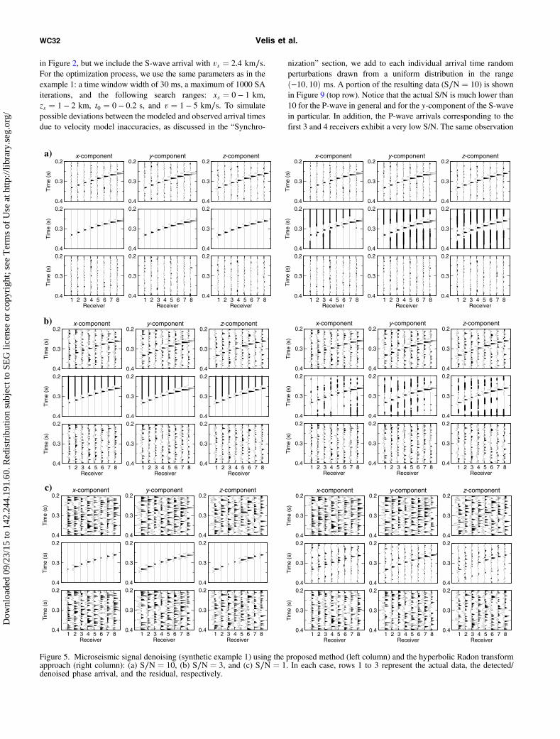
As for the denoising stage, the results are shown in Figure 5 (leftcolumn) for a particular realization of those averaged in Table 1. Ineach case, we use a single eigenimage to approximate the datawithin the final search window. We observe that the waveforms andamplitudes were recovered very well, especially for the higher S/Ncases (Figure 5a and 5b, left column). In these cases, the normalizedcrosscorrelations between the noise-free data sets and the corre-sponding denoised data sets are very high (greater than 0.95), asshown in Table 2. Although less accurately, the microseismic signalwas also recovered in the very low S/N case (Figure 5c, left col-umn). Overall, these results are quite reasonable, considering thefact that the actual signal is badly contaminated in the S∕N ¼ 3 case(Figure 5b, left column), and they are almost undistinguished (if nothidden at all) in the S∕N ¼ 1 case (Figure 5c, left column).For comparison, Figure 5 (right column) shows the results of the

detection and denoising using the apex-shifted hyperbolic Radontransform approach described in Sabbione et al. (2013). For thetwo higher S/N cases, we observe that the accuracy of the resultsis very similar to the accuracy obtained using the proposed SVDfiltering, yielding very high crosscorrelation values (see Table 2).However, the Radon approach degrades significantly in the verylow S/N case. Note that for a fair comparison, we calculate thecrosscorrelations using the denoised images muted with the samehyperbolic window used in the SVD filtering.Figure 6 shows the convergence curves for the S∕N ¼ 3 case

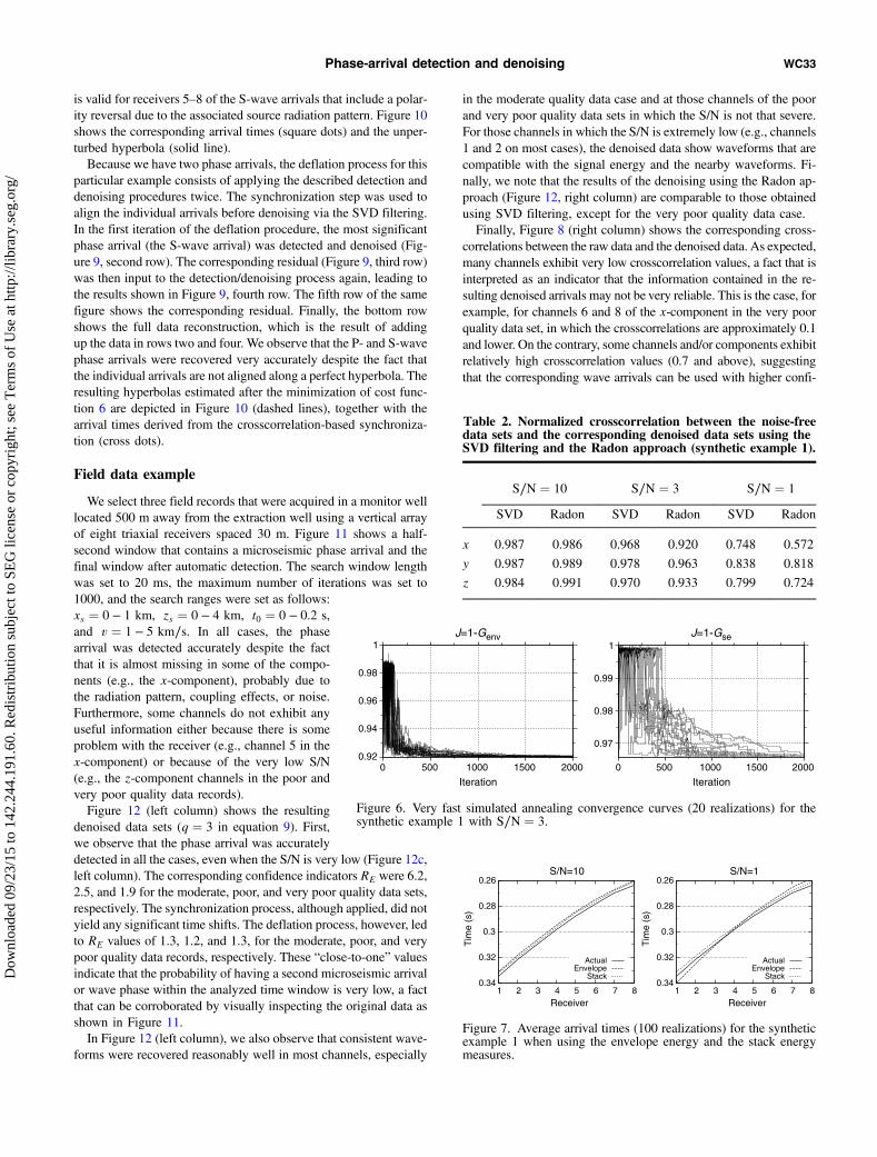
(synthetic example 1), using the envelope energy Genv (left panel)and the stack energy Gse (right panel), respectively. Note that inmost cases, the convergence is achieved well before 1000 iterations,especially when G ¼ Genv. The convergence is faster when usingthe envelope energy measure because it is smoother (and easier tominimize/maximize) than the stack energy measure (see Figures 3and 4). The same behavior is observed for the cases with S∕N ¼ 10

and 1 (not shown). In terms of computational cost, the final solutionfor a single SA run using either measure is obtained almost instantlyon a standard PC, making the method suitable for real-timeprocessing.When we compare the arrival times plotted in Figure 7, we notice

that, due to its higher resolving power, the greater accuracy is ob-tained when using the stack energy (dotted line) than using theenvelope energy (dashed line) in the S∕N ¼ 1 case (Figure 7, rightpanel). However, when the noise level is moderate to low (S∕N ¼ 10,left panel of the same figure), both measures exhibit similar accuracy,in spite of a relatively small bias of a few milliseconds. We want tostress that for the sake of the phase-arrival detection process, bothmeasures behave satisfactorily well, even for the S∕N ¼ 1 case, inwhich the signal is almost indistinguishable. Nonetheless, for theSVD filtering, it is clear that we need to obtain a hyperbolic windowthat follows as closely as possible the curvature of the actual phasearrival. A moderate bias is of no concern because the individualwaveforms would add up in phase anyway. On the contrary, anydeviation from the actual curvature, as shown in the right panelof Figure 7 for the envelope-energy case, would certainly diminishthe quality of the results.Quantitatively, the accuracy of the results was already assessed

by analyzing the normalized crosscorrelations between the clean(noise free) data and the denoised data as shown in Table 2. Becausethe clean data are not available when dealing with field data sets, theaccuracy of the results can be assessed by analyzing, instead, thenormalized crosscorrelations between the raw (noisy) and thedenoised data. Theses quantities are depicted in Figure 8 (left col-umn), on a channel-by-channel basis. Note that crosscorrelation val-ues greater than 0.7–0.8 are obtained for most microseismic arrivals,except for the very low S/N case. Crosscorrelation between the ac-tual and the denoised signals is viewed as an S/N indicator that canbe used for subsequent microseismic data analysis processes. Forexample, they could be used as weights when averaging the indi-vidual azimuths derived from a hodogram analysis.

Synthetic example 2

The purpose of the second synthetic example is to test the syn-chronization and deflation processes. This example illustrates thecase in which the underlying velocity model is not constant andthere is more than a single phase arrival. Essentially, we use thesame source-receiver geometry as in the case of the data shown

Table 1. Mean and standard deviation after 100 realizations(kmax � 1000, G � Gse). Actual event parameters are�xs; zs; t0; v� � �0.5; 1.6; 0.0; 3.0�.

S∕N ¼ 10 S∕N ¼ 3 S∕N ¼ 1

xs (km) 0.534� 0.122 0.531� 0.126 0.467� 0.110

zs (km) 1.648� 0.086 1.640� 0.092 1.680� 0.161

t0 (s) 0.002� 0.054 0.000� 0.057 −0.003� 0.050

v (km∕s) 3.139� 0.411 3.068� 0.420 2.901� 0.568

Δtrms (s) 0.0031� 0.0016 0.0039� 0.0021 0.0044� 0.0009

G 0.0698� 0.0007 0.0079� 0.0008 0.1050� 0.0011

RE 9.17� 1.67 3.67� 0.29 1.39� 0.10

Phase-arrival detection and denoising WC31

Dow

nloa

ded

09/2

3/15

to 1

42.2

44.1

91.6

0. R

edis

trib

utio

n su

bjec

t to

SEG

lice

nse

or c

opyr

ight

; see

Ter

ms

of U

se a

t http

://lib

rary

.seg

.org

/

in Figure 2, but we include the S-wave arrival with vs ¼ 2.4 km∕s.For the optimization process, we use the same parameters as in theexample 1: a time window width of 30 ms, a maximum of 1000 SAiterations, and the following search ranges: xs ¼ 0 − 1 km,zs ¼ 1 − 2 km, t0 ¼ 0 − 0.2 s, and v ¼ 1 − 5 km∕s. To simulatepossible deviations between the modeled and observed arrival timesdue to velocity model inaccuracies, as discussed in the “Synchro-

nization” section, we add to each individual arrival time randomperturbations drawn from a uniform distribution in the rangeð−10; 10Þ ms. A portion of the resulting data (S∕N ¼ 10) is shownin Figure 9 (top row). Notice that the actual S/N is much lower than10 for the P-wave in general and for the y-component of the S-wavein particular. In addition, the P-wave arrivals corresponding to thefirst 3 and 4 receivers exhibit a very low S/N. The same observation

0.2

0.3

0.4

Tim

e (s

)

x-componenta) 0.2

0.3

0.4

y-component 0.2

0.3

0.4

z-component

0.2

0.3

0.4

Tim

e (s

)

0.2

0.3

0.4

0.2

0.3

0.4 0.2

0.3

0.4 1 2 3 4 5 6 7 8

Tim

e (s

)

Receiver

0.2

0.3

0.4 1 2 3 4 5 6 7 8

Receiver

0.2

0.3

0.4 1 2 3 4 5 6 7 8

Receiver

0.2

0.3

0.4

Tim

e (s

)

x-component 0.2

0.3

0.4

y-component 0.2

0.3

0.4

z-component

0.2

0.3

0.4

Tim

e (s

)

0.2

0.3

0.4

0.2

0.3

0.4 0.2

0.3

0.4 1 2 3 4 5 6 7 8

Tim

e (s

)

Receiver

0.2

0.3

0.4 1 2 3 4 5 6 7 8

Receiver

0.2

0.3

0.4 1 2 3 4 5 6 7 8

Receiver

0.2

0.3

0.4

Tim

e (s

)

x-componentb) 0.2

0.3

0.4

y-component 0.2

0.3

0.4

z-component

0.2

0.3

0.4

Tim

e (s

)

0.2

0.3

0.4

0.2

0.3

0.4 0.2

0.3

0.4 1 2 3 4 5 6 7 8

Tim

e (s

)

Receiver

0.2

0.3

0.4 1 2 3 4 5 6 7 8

Receiver

0.2

0.3

0.4 1 2 3 4 5 6 7 8

Receiver

0.2

0.3

0.4

Tim

e (s

)

x-component 0.2

0.3

0.4

y-component 0.2

0.3

0.4

z-component

0.2

0.3

0.4

Tim

e (s

)

0.2

0.3

0.4

0.2

0.3

0.4 0.2

0.3

0.4 1 2 3 4 5 6 7 8

Tim

e (s

)

Receiver

0.2

0.3

0.4 1 2 3 4 5 6 7 8

Receiver

0.2

0.3

0.4 1 2 3 4 5 6 7 8

Receiver

0.2

0.3

0.4

Tim

e (s

)

x-componentc) 0.2

0.3

0.4

y-component 0.2

0.3

0.4

z-component

0.2

0.3

0.4

Tim

e (s

)

0.2

0.3

0.4

0.2

0.3

0.4 0.2

0.3

0.4 1 2 3 4 5 6 7 8

Tim

e (s

)

Receiver

0.2

0.3

0.4 1 2 3 4 5 6 7 8

Receiver

0.2

0.3

0.4 1 2 3 4 5 6 7 8

Receiver

0.2

0.3

0.4

Tim

e (s

)

x-component 0.2

0.3

0.4

y-component 0.2

0.3

0.4

z-component

0.2

0.3

0.4

Tim

e (s

)

0.2

0.3

0.4

0.2

0.3

0.4 0.2

0.3

0.4 1 2 3 4 5 6 7 8

Tim

e (s

)

Receiver

0.2

0.3

0.4 1 2 3 4 5 6 7 8

Receiver

0.2

0.3

0.4 1 2 3 4 5 6 7 8

Receiver

Figure 5. Microseismic signal denoising (synthetic example 1) using the proposed method (left column) and the hyperbolic Radon transformapproach (right column): (a) S∕N ¼ 10, (b) S∕N ¼ 3, and (c) S∕N ¼ 1. In each case, rows 1 to 3 represent the actual data, the detected/denoised phase arrival, and the residual, respectively.

WC32 Velis et al.

Dow

nloa

ded

09/2

3/15

to 1

42.2

44.1

91.6

0. R

edis

trib

utio

n su

bjec

t to

SEG

lice

nse

or c

opyr

ight

; see

Ter

ms

of U

se a

t http

://lib

rary

.seg

.org

/

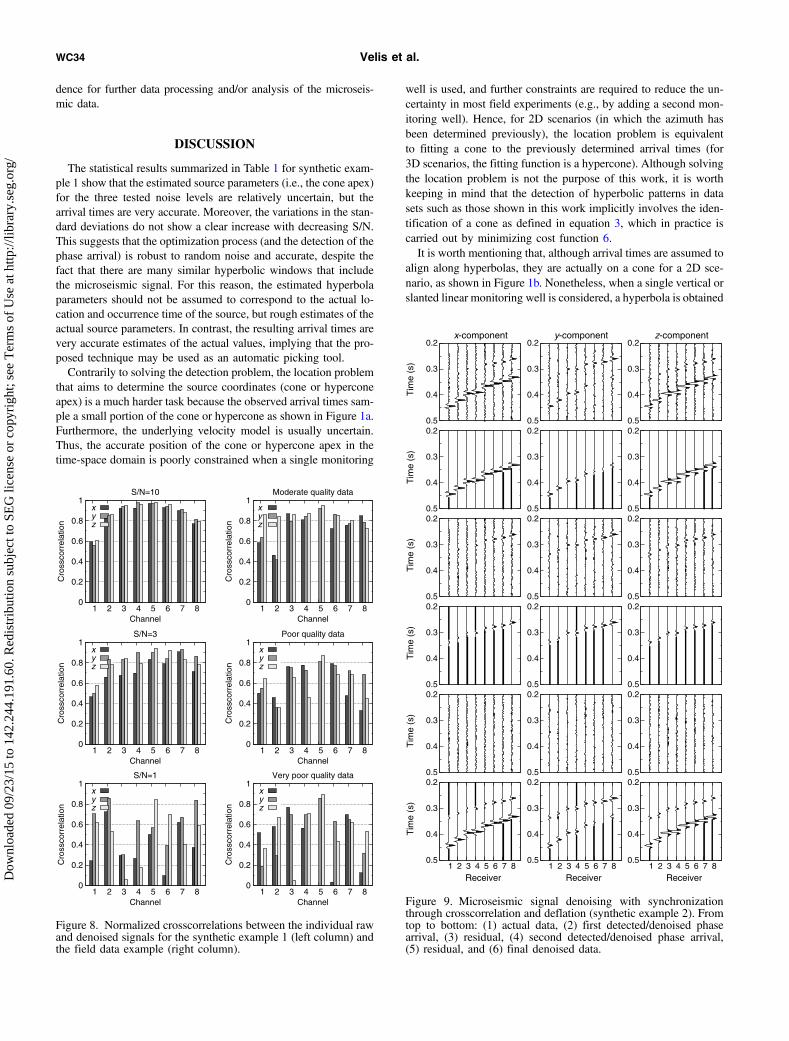
is valid for receivers 5–8 of the S-wave arrivals that include a polar-ity reversal due to the associated source radiation pattern. Figure 10shows the corresponding arrival times (square dots) and the unper-turbed hyperbola (solid line).Because we have two phase arrivals, the deflation process for this

particular example consists of applying the described detection anddenoising procedures twice. The synchronization step was used toalign the individual arrivals before denoising via the SVD filtering.In the first iteration of the deflation procedure, the most significantphase arrival (the S-wave arrival) was detected and denoised (Fig-ure 9, second row). The corresponding residual (Figure 9, third row)was then input to the detection/denoising process again, leading tothe results shown in Figure 9, fourth row. The fifth row of the samefigure shows the corresponding residual. Finally, the bottom rowshows the full data reconstruction, which is the result of addingup the data in rows two and four. We observe that the P- and S-wavephase arrivals were recovered very accurately despite the fact thatthe individual arrivals are not aligned along a perfect hyperbola. Theresulting hyperbolas estimated after the minimization of cost func-tion 6 are depicted in Figure 10 (dashed lines), together with thearrival times derived from the crosscorrelation-based synchroniza-tion (cross dots).

Field data example

We select three field records that were acquired in a monitor welllocated 500 m away from the extraction well using a vertical arrayof eight triaxial receivers spaced 30 m. Figure 11 shows a half-second window that contains a microseismic phase arrival and thefinal window after automatic detection. The search window lengthwas set to 20 ms, the maximum number of iterations was set to1000, and the search ranges were set as follows:xs ¼ 0 − 1 km, zs ¼ 0 − 4 km, t0 ¼ 0 − 0.2 s,and v ¼ 1 − 5 km∕s. In all cases, the phasearrival was detected accurately despite the factthat it is almost missing in some of the compo-nents (e.g., the x-component), probably due tothe radiation pattern, coupling effects, or noise.Furthermore, some channels do not exhibit anyuseful information either because there is someproblem with the receiver (e.g., channel 5 in thex-component) or because of the very low S/N(e.g., the z-component channels in the poor andvery poor quality data records).Figure 12 (left column) shows the resulting

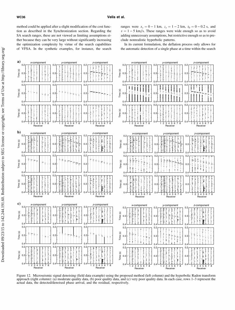
denoised data sets (q ¼ 3 in equation 9). First,we observe that the phase arrival was accuratelydetected in all the cases, even when the S/N is very low (Figure 12c,left column). The corresponding confidence indicators RE were 6.2,2.5, and 1.9 for the moderate, poor, and very poor quality data sets,respectively. The synchronization process, although applied, did notyield any significant time shifts. The deflation process, however, ledto RE values of 1.3, 1.2, and 1.3, for the moderate, poor, and verypoor quality data records, respectively. These “close-to-one” valuesindicate that the probability of having a second microseismic arrivalor wave phase within the analyzed time window is very low, a factthat can be corroborated by visually inspecting the original data asshown in Figure 11.In Figure 12 (left column), we also observe that consistent wave-

forms were recovered reasonably well in most channels, especially

in the moderate quality data case and at those channels of the poorand very poor quality data sets in which the S/N is not that severe.For those channels in which the S/N is extremely low (e.g., channels1 and 2 on most cases), the denoised data show waveforms that arecompatible with the signal energy and the nearby waveforms. Fi-nally, we note that the results of the denoising using the Radon ap-proach (Figure 12, right column) are comparable to those obtainedusing SVD filtering, except for the very poor quality data case.Finally, Figure 8 (right column) shows the corresponding cross-

correlations between the raw data and the denoised data. As expected,many channels exhibit very low crosscorrelation values, a fact that isinterpreted as an indicator that the information contained in the re-sulting denoised arrivals may not be very reliable. This is the case, forexample, for channels 6 and 8 of the x-component in the very poorquality data set, in which the crosscorrelations are approximately 0.1and lower. On the contrary, some channels and/or components exhibitrelatively high crosscorrelation values (0.7 and above), suggestingthat the corresponding wave arrivals can be used with higher confi-

Table 2. Normalized crosscorrelation between the noise-freedata sets and the corresponding denoised data sets using theSVD filtering and the Radon approach (synthetic example 1).

S∕N ¼ 10 S∕N ¼ 3 S∕N ¼ 1

SVD Radon SVD Radon SVD Radon

x 0.987 0.986 0.968 0.920 0.748 0.572

y 0.987 0.989 0.978 0.963 0.838 0.818

z 0.984 0.991 0.970 0.933 0.799 0.724

0.92

0.94

0.96

0.98

1

0 500 1000 1500 2000

Iteration

J=1-Genv

0.97

0.98

0.99

1

0 500 1000 1500 2000

Iteration

J=1-Gse

Figure 6. Very fast simulated annealing convergence curves (20 realizations) for thesynthetic example 1 with S∕N ¼ 3.

0.26

0.28

0.3

0.32

0.34 1 2 3 4 5 6 7 8

Tim

e (s

)

Receiver

S/N=10

ActualEnvelope

Stack

0.26

0.28

0.3

0.32

0.34 1 2 3 4 5 6 7 8

Tim

e (s

)

Receiver

S/N=1

ActualEnvelope

Stack

Figure 7. Average arrival times (100 realizations) for the syntheticexample 1 when using the envelope energy and the stack energymeasures.

Phase-arrival detection and denoising WC33

Dow

nloa

ded

09/2

3/15

to 1

42.2

44.1

91.6

0. R

edis

trib

utio

n su

bjec

t to

SEG

lice

nse

or c

opyr

ight

; see

Ter

ms

of U

se a

t http

://lib

rary

.seg

.org

/

dence for further data processing and/or analysis of the microseis-mic data.

DISCUSSION

The statistical results summarized in Table 1 for synthetic exam-ple 1 show that the estimated source parameters (i.e., the cone apex)for the three tested noise levels are relatively uncertain, but thearrival times are very accurate. Moreover, the variations in the stan-dard deviations do not show a clear increase with decreasing S/N.This suggests that the optimization process (and the detection of thephase arrival) is robust to random noise and accurate, despite thefact that there are many similar hyperbolic windows that includethe microseismic signal. For this reason, the estimated hyperbolaparameters should not be assumed to correspond to the actual lo-cation and occurrence time of the source, but rough estimates of theactual source parameters. In contrast, the resulting arrival times arevery accurate estimates of the actual values, implying that the pro-posed technique may be used as an automatic picking tool.Contrarily to solving the detection problem, the location problem

that aims to determine the source coordinates (cone or hyperconeapex) is a much harder task because the observed arrival times sam-ple a small portion of the cone or hypercone as shown in Figure 1a.Furthermore, the underlying velocity model is usually uncertain.Thus, the accurate position of the cone or hypercone apex in thetime-space domain is poorly constrained when a single monitoring

well is used, and further constraints are required to reduce the un-certainty in most field experiments (e.g., by adding a second mon-itoring well). Hence, for 2D scenarios (in which the azimuth hasbeen determined previously), the location problem is equivalentto fitting a cone to the previously determined arrival times (for3D scenarios, the fitting function is a hypercone). Although solvingthe location problem is not the purpose of this work, it is worthkeeping in mind that the detection of hyperbolic patterns in datasets such as those shown in this work implicitly involves the iden-tification of a cone as defined in equation 3, which in practice iscarried out by minimizing cost function 6.It is worth mentioning that, although arrival times are assumed to

align along hyperbolas, they are actually on a cone for a 2D sce-nario, as shown in Figure 1b. Nonetheless, when a single vertical orslanted linear monitoring well is considered, a hyperbola is obtained

0

0.2

0.4

0.6

0.8

1

1 2 3 4 5 6 7 8

Cro

ssco

rrel

atio

n

Channel

S/N=10

xyz

0

0.2

0.4

0.6

0.8

1

1 2 3 4 5 6 7 8

Cro

ssco

rrel

atio

n

Channel

Moderate quality data

xyz

0

0.2

0.4

0.6

0.8

1

1 2 3 4 5 6 7 8

Cro

ssco

rrel

atio

n

Channel

S/N=3

xyz

0

0.2

0.4

0.6

0.8

1

1 2 3 4 5 6 7 8

Cro

ssco

rrel

atio

n

Channel

Poor quality data

xyz

0

0.2

0.4

0.6

0.8

1

1 2 3 4 5 6 7 8

Cro

ssco

rrel

atio

n

Channel

S/N=1

xyz

0

0.2

0.4

0.6

0.8

1

1 2 3 4 5 6 7 8

Cro

ssco

rrel

atio

n

Channel

Very poor quality data

xyz

Figure 8. Normalized crosscorrelations between the individual rawand denoised signals for the synthetic example 1 (left column) andthe field data example (right column).

0.2

0.3

0.4

0.5T

ime

(s)

x-component 0.2

0.3

0.4

0.5

y-component 0.2

0.3

0.4

0.5

z-component

0.2

0.3

0.4

0.5

Tim

e (s

)

0.2

0.3

0.4

0.5

0.2

0.3

0.4

0.5 0.2

0.3

0.4

0.5

Tim

e (s

)

0.2

0.3

0.4

0.5

0.2

0.3

0.4

0.5 0.2

0.3

0.4

0.5

Tim

e (s

)

0.2

0.3

0.4

0.5

0.2

0.3

0.4

0.5 0.2

0.3

0.4

0.5

Tim

e (s

)

0.2

0.3

0.4

0.5

0.2

0.3

0.4

0.5 0.2

0.3

0.4

0.5 1 2 3 4 5 6 7 8

Tim

e (s

)

Receiver

0.2

0.3

0.4

0.5 1 2 3 4 5 6 7 8

Receiver

0.2

0.3

0.4

0.5 1 2 3 4 5 6 7 8

Receiver

Figure 9. Microseismic signal denoising with synchronizationthrough crosscorrelation and deflation (synthetic example 2). Fromtop to bottom: (1) actual data, (2) first detected/denoised phasearrival, (3) residual, (4) second detected/denoised phase arrival,(5) residual, and (6) final denoised data.

WC34 Velis et al.

Dow

nloa

ded

09/2

3/15

to 1

42.2

44.1

91.6

0. R

edis

trib

utio

n su

bjec

t to

SEG

lice

nse

or c

opyr

ight

; see

Ter

ms

of U

se a

t http

://lib

rary

.seg

.org

/

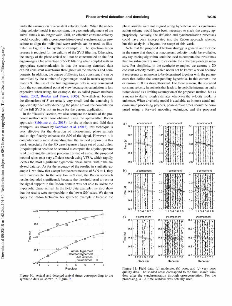
under the assumption of a constant velocity model. When the under-lying velocity model is not constant, the geometric alignment of thearrival times is no longer valid. Still, an effective constant-velocitymodel coupled with a crosscorrelation-based synchronization pro-cedure to align the individual wave arrivals can be used, as illus-trated in Figure 9 for synthetic example 2. The synchronizationprocess is required for the validity of the SVD filtering. Otherwise,the energy of the phase arrival will not be concentrated on the firsteigenimages. One advantage of SVD filtering when coupled with anappropriate synchronization is that the resulting denoised dataexhibit consistent waveforms throughout all the channels and com-ponents. In addition, the degree of filtering (and consistency) can becontrolled by the number of eigenimages used in matrix approxi-mation 9. The use of the first eigenimage only is very convenientfrom the computational point of view because its calculation is lessexpensive when using, for example, the so-called power methods(Antia, 2002; Burden and Faires, 2005). Nevertheless, becausethe dimensions of S are usually very small, and the denoising isapplied only once after detecting the phase arrival, the computationof the full SVD is not an issue for the current application.In the “Results” section, we also compare the results of the pro-

posed method with those obtained using the apex-shifted Radonapproach (Sabbione et al., 2013), for the synthetic and field dataexamples. As shown by Sabbione et al. (2013), this technique isvery effective for the detection of microseismic phase arrivalsand to significantly enhance the S/N of the signal. However, it iscomputationally more demanding than the method proposed in thiswork, especially for the 3D case because a large set of quadruplets(or quintuplets) needs to be scanned to compute the adjoint operatorused in solving the inverse problem. Instead of a scan, the proposedmethod relies on a very efficient search using VFSA, which rapidlylocates the most significant hyperbolic phase arrival within the an-alyzed data set. As for the accuracy of the results, in synthetic ex-ample 1, we show that except for the extreme case of S∕N ¼ 1, theywere comparable. In the very low S/N case, the Radon approachresults degraded significantly because the threshold used to restrictthe signal support in the Radon domain was not able to isolate thehyperbolic phase arrival. In the field data example, we also showthat the results were comparable in the lower S/N cases. We do notapply the Radon technique for synthetic example 2 because the

phase arrivals were not aligned along hyperbolas and a synchroni-zation scheme would have been necessary to stack the energy ap-propriately. Actually, the deflation and synchronization processescould have been incorporated into the Radon approach scheme,but this analysis is beyond the scope of this work.Note that the proposed detection strategy is general and flexible

in the sense that should a nonconstant velocity model be available,any ray-tracing algorithm could be used to compute the traveltimesthat are subsequently used to calculate the coherency-energy mea-sure. For simplicity, in the synthetic examples, we assume a 2Dconstant velocity model, which needs not be known a priori becauseit represents an unknown to be determined together with the param-eters that define the corresponding hyperbola. In this context, theextension to 3D is straightforward. For these reasons, the so-calledconstant velocity hypothesis that leads to hyperbolic integration pathsis not viewed as a limiting assumption of the proposed method, but asa means to derive rough estimates whenever the velocity model isunknown. When a velocity model is available, as in most actual mi-croseismic processing projects, phase-arrival times should be com-puted using a forward modeling technique, and the proposed

0.1

0.2

0.3

0.4

0.5 1 2 3 4 5 6 7 8

Tim

e (s

)

Receiver

x-componentc) 0.1

0.2

0.3

0.4

0.5 1 2 3 4 5 6 7 8

Receiver

y-component 0.1

0.2

0.3

0.4

0.5 1 2 3 4 5 6 7 8

Receiver

z-component

0.1

0.2

0.3

0.4

0.5 1 2 3 4 5 6 7 8

Tim

e (s

)

x-componentb) 0.1

0.2

0.3

0.4

0.5 1 2 3 4 5 6 7 8

y-component 0.1

0.2

0.3

0.4

0.5 1 2 3 4 5 6 7 8

z-component

0.1

0.2

0.3

0.4

0.5 1 2 3 4 5 6 7 8

Tim

e (s

)x-componenta)

0.1

0.2

0.3

0.4

0.5 1 2 3 4 5 6 7 8

y-component 0.1

0.2

0.3

0.4

0.5 1 2 3 4 5 6 7 8

z-component

Figure 11. Field data: (a) moderate, (b) poor, and (c) very poorquality data. The shaded areas correspond to the final search win-dow after the synchronization through crosscorrelation. For theprocessing, a 1-s time window was actually used.

0.25

0.3

0.35

0.4

0.45 1 2 3 4 5 6 7 8

Tim

e (s

)

Receiver

Actual hyperbolaDetected hyperbola

Actual timesPicked times

Figure 10. Actual and detected arrival times corresponding to thesynthetic data as shown in Figure 9.

Phase-arrival detection and denoising WC35

Dow

nloa

ded

09/2

3/15

to 1

42.2

44.1

91.6

0. R

edis

trib

utio

n su

bjec

t to

SEG

lice

nse

or c

opyr

ight

; see

Ter

ms

of U

se a

t http

://lib

rary

.seg

.org

/

method could be applied after a slight modification of the cost func-tion as described in the Synchronization section. Regarding theSA search ranges, these are not viewed as limiting assumptions ei-ther because they can be very large without significantly increasingthe optimization complexity by virtue of the search capabilitiesof VFSA. In the synthetic examples, for instance, the search

ranges were xs ¼ 0 − 1 km, zs ¼ 1 − 2 km, t0 ¼ 0 − 0.2 s, andv ¼ 1 − 5 km∕s. These ranges were wide enough so as to avoidadding unnecessary assumptions, but restrictive enough so as to pre-clude nonrealistic hyperbolic patterns.In its current formulation, the deflation process only allows for

the automatic detection of a single phase at a time within the search

0.2

0.3

0.4

Tim

e (s

)

x-componenta) 0.2

0.3

0.4

y-component 0.2

0.3

0.4

z-component

0.2

0.3

0.4

Tim

e (s

)

0.2

0.3

0.4

0.2

0.3

0.4 0.2

0.3

0.4 1 2 3 4 5 6 7 8

Tim

e (s

)

Receiver

0.2

0.3

0.4 1 2 3 4 5 6 7 8

Receiver

0.2

0.3

0.4 1 2 3 4 5 6 7 8

Receiver

0.2

0.3

0.4

Tim

e (s

)

x-component 0.2

0.3

0.4

y-component 0.2

0.3

0.4

z-component

0.2

0.3

0.4

Tim

e (s

)

0.2

0.3

0.4

0.2

0.3

0.4 0.2

0.3

0.4 1 2 3 4 5 6 7 8

Tim

e (s

)

Receiver

0.2

0.3

0.4 1 2 3 4 5 6 7 8

Receiver

0.2

0.3

0.4 1 2 3 4 5 6 7 8

Receiver

0.2

0.3

0.4

Tim

e (s

)

x-componentb) 0.2

0.3

0.4

y-component 0.2

0.3

0.4

z-component

0.2

0.3

0.4

Tim

e (s

)

0.2

0.3

0.4

0.2

0.3

0.4 0.2

0.3

0.4 1 2 3 4 5 6 7 8

Tim

e (s

)

Receiver

0.2

0.3

0.4 1 2 3 4 5 6 7 8

Receiver

0.2

0.3

0.4 1 2 3 4 5 6 7 8

Receiver

0.2

0.3

0.4

Tim

e (s

)

x-component 0.2

0.3

0.4

y-component 0.2

0.3

0.4

z-component

0.2

0.3

0.4

Tim

e (s

)

0.2

0.3

0.4

0.2

0.3

0.4 0.2

0.3

0.4 1 2 3 4 5 6 7 8

Tim

e (s

)

Receiver

0.2

0.3

0.4 1 2 3 4 5 6 7 8

Receiver

0.2

0.3

0.4 1 2 3 4 5 6 7 8

Receiver

0.2

0.3

0.4

Tim

e (s

)

x-componentc) 0.2

0.3

0.4

y-component 0.2

0.3

0.4

z-component

0.2

0.3

0.4

Tim

e (s

)

0.2

0.3

0.4

0.2

0.3

0.4 0.2

0.3

0.4 1 2 3 4 5 6 7 8

Tim

e (s

)

Receiver

0.2

0.3

0.4 1 2 3 4 5 6 7 8

Receiver

0.2

0.3

0.4 1 2 3 4 5 6 7 8

Receiver

0.2

0.3

0.4

Tim

e (s

)

x-component 0.2

0.3

0.4

y-component 0.2

0.3

0.4

z-component

0.2

0.3

0.4

Tim

e (s

)

0.2

0.3

0.4

0.2

0.3

0.4 0.2

0.3

0.4 1 2 3 4 5 6 7 8

Tim

e (s

)

Receiver

0.2

0.3

0.4 1 2 3 4 5 6 7 8

Receiver

0.2

0.3

0.4 1 2 3 4 5 6 7 8

Receiver

Figure 12. Microseismic signal denoising (field data example) using the proposed method (left column) and the hyperbolic Radon transformapproach (right column): (a) moderate quality data, (b) poor quality data, and (c) very poor quality data. In each case, rows 1–3 represent theactual data, the detected/denoised phase arrival, and the residual, respectively.

WC36 Velis et al.

Dow

nloa

ded

09/2

3/15

to 1

42.2

44.1

91.6

0. R

edis

trib

utio

n su

bjec

t to

SEG

lice

nse

or c

opyr

ight

; see

Ter

ms

of U

se a

t http

://lib

rary

.seg

.org

/

window (P- or S-wave splitting). This means that some extra workis required to identify the different detected phase arrivals andassociate them with one or more microseismic events. There arevarious strategies that can be implemented to solve this problem. Inthe case that the P- and S-wave velocity models are available, themethod can be easily modified to search for two (or three) hyper-bolas simultaneously (one for each phase arrival). To this end, onewould have to redefine the coherence function G as the sum of thecoherence functions associated to each potential phase arrival. Thisimplementation is straightforward. Another option would be to addextra unknowns to account for the P- and S-wave velocities underthe constant effective velocity assumption, and do the same. Sim-ilarly, when there are two or more monitoring wells, there would beone hyperbolic pattern associated with each phase arrival and mon-itoring well. Then, the contribution of all the hyperbolic patternswould have to be added altogether into a single coherence function.The key difference is that the hyperbolas for each monitor well thatare associated with the same phase arrival would share the samesource coordinates and origin time.

CONCLUSIONS

The proposed technique allows one to automatically detect anddenoise a microseismic phase arrival immersed in 3C noisy data.The technique is fast and accurate, provided a constant velocitymodel is appropriate to define the alignment of the arrivals alongan hyperbola. For nonconstant velocity models, the proposed cross-correlation-based synchronization process allows one to detect andappropriately denoise nonhyperbolic phase arrivals. In this context,SVD filtering promotes consistent waveforms throughout all thechannels and components, independently of the regularity observedin the alignment of the time arrivals. Furthermore, a crosscorrela-tion-based S/N indicator is provided to assess the significance of thereconstructed individual arrivals. This indicator could be used as aweighting factor for further processing and/or analysis of the micro-seismic data.A deflation process is proposed to handle more than a single

phase arrival within the analyzed time window. The deflation proc-ess is iterative, leading to a sequence of detected and denoised phasearrivals of decreasing energy that is repeated until the residual datacontain no significant coherent energy. A simple energy-ratio con-fidence indicator that prevents the detection of false positives is pro-vided for this purpose.The detection-denoising strategy is very simple because the tun-

ing parameters are just a few and easily set. These include the maxi-mum number of VFSA iterations and the length of the time windowassociated with the hyperbola. In particular, we used 1000 iterationsin all the examples for data windows of 0.5–1 s and a hyperbolicsearch window of 20–30 ms, just enough to encompass one periodof the expected signal arrival.Tests using synthetic and field data demonstrated that the proposed

technique behaved very accurately when applied to moderate- tohigh-S/N data sets, and reasonably well when applied to very noisydata sets. The algorithm output includes the following: (1) estimatesof the origin time, coordinates of the source, an effective velocitymodel, and the corresponding traveltimes, (2) consistent denoisedwave arrivals throughout all the channels and components, and(3) two confidence indicators: one to asses the presence of an actualphase arrival, and the other to assess the reliability of the derivedwave arrivals. Overall, the detection is robust to random noise, the

derived traveltimes are accurate, and the denoised waveforms areconsistent with the observed data.

ACKNOWLEDGMENTS

We thank the editor and the three reviewers for their commentsand suggestions that helped to improve our manuscript. This workwas partially financed by Agencia Nacional de Promoción Científ-ica y Tecnológica, Argentina (PICT 2010-2129).

REFERENCES

Antia, H., 2002, Numerical methods for scientists and engineers 2nd ed.:Tata McGraw Hill.

Blias, E., and V. Grechka, 2013, Analytic solutions to the joint estimation ofmicroseismic event locations and effective velocity model: Geophysics,78, no. 3, KS51–KS61, doi: 10.1190/geo2012-0517.1.

Burden, R. L., and J. D. Faires, 2005, Numerical analysis 8th ed.: ThomsonBrooks/Cole.

Chen, Z., and R. Stewart, 2006, A multi-window algorithm for real-timeautomatic detection and picking of P-phases of seismic events: CREWESResearch Report, 18, 15.1–15.9.

Chopra, S., and K. Marfurt, 2007, Seismic attributes for prospect identifi-cation and reservoir characterization 1st ed.: SEG, Geophysical Develop-ments 11.

DiCarlo, J. J., D. Zoccolan, and N. C. Rust, 2012, How does the brain solvevisual object recognition?: Neuron, 73, 415–434, doi: 10.1016/j.neuron.2012.01.010.

Eisner, L., B. Hulsey, P. Duncan, D. Jurick, H. Werner, and W. Keller, 2010,Comparison of surface and borehole locations of induced microseismic-ity: Geophysical Prospecting, 58, 809–820, doi: 10.1111/j.1365-2478.2010.00867.x.

Felleman, D. J., and D. van Essen, 1991, Distributed hierarchical processingin the primate cerebral cortex: Cerebral Cortex, 1, 1–47, doi: 10.1093/cercor/1.1.1-a.

Galotti, K. M., 2014, Cognitive psychology: In and out of the laboratory (5thed.): SAGE Publications, Inc.

Gharti, H. N., V. Oye, M. Roth, and D. Kühn, 2010, Automatedmicroearthquake location using envelope stacking and robust global op-timization: Geophysics, 75, no. 4, MA27–MA46, doi: 10.1190/1.3432784.

Golub, G., and C. Van Loan, 1989, Matrix computations 2nd ed.: JohnsHopkins University Press.

Gonzalez, R. C., and R. E. Wood, 2007, Digital image processing 3rd ed.:Prentice Hall.

Ingber, L., 1989, Very fast simulated re-annealing: Journal of MathematicalComputation and Modelling, 12, 967–973, doi: 10.1016/0895-7177(89)90202-1.

Kendall, M., S. Maxwell, G. Foulger, L. Eisner, and Z. Lawrence,2011, Special section. Microseismicity: Beyond dots in a box — Intro-duction: Geophysics, 76, no. 6, WC1–WC3, doi: 10.1190/geo-2011-1114-SPSEIN.1.

Lagos, S. R., J. I. Sabbione, and D. R. Velis, 2014, Very fast simulatedannealing and particle swarm optimization for microseismic event loca-tion: 84th Annual International Meeting, SEG, Expanded Abstracts,2188–2192.

Liu, J., and K. Marfurt, 2005, Matching pursuit decomposition using Morletwavelet: 75th Annual International Meeting, SEG, Expanded Abstracts,786–789.

Mallat, S., and Z. Zhang, 1993, Matching pursuit with time-frequency dic-tionaries: IEEE Transactions on Signal Processing, 41, 3397–3415, doi:10.1109/78.258082.

Maxwell, S., 2014, Microseismic imaging of hydraulic fracturing: Improvedengineering of unconventional shale reservoirs: SEG, Distinguished In-structor Series, 17.

Maxwell, S. C., J. Rutledge, R. Jones, and M. Fehler, 2010, Petroleum res-ervoir characterization using downhole microseismic monitoring: Geo-physics, 75, no. 5, 75A129–75A137, doi: 10.1190/1.3477966.

Michaud, G., and S. Leaney, 2008, Continuous microseismic mapping forreal-time event detection and location: 78th Annual International Meeting,SEG, Expanded Abstracts, 1357–1361.

Munro, K., 2004, Automatic event detection and picking of P-wave arrivals:CREWES Research Report, 16, 12.1–12.10.

Neidell, N., and M. T. Taner, 1971, Semblance and other coherency mea-sures for multichannel data: Geophysics, 36, 482–497, doi: 10.1190/1.1440186.

Phase-arrival detection and denoising WC37

Dow

nloa

ded

09/2

3/15

to 1

42.2

44.1

91.6

0. R

edis

trib

utio

n su

bjec

t to

SEG

lice

nse

or c

opyr

ight

; see

Ter

ms

of U

se a

t http

://lib

rary

.seg

.org

/

Press, W. H., S. Teukolsky, W. Vetterling, and B. Flannery, 1992, Numericalrecipes in FORTRAN: The art of scientific computing 2nd ed.: CambridgeUniversity Press.

Sabbione, J., M. D. Sacchi, and D. R. Velis, 2015, Radon transform-basedmicroseismic event detection and signal-to-noise ratio enhancement:Journal of Applied Geophysics, 113, 51–63, doi: 10.1016/j.jappgeo.2014.12.008.

Sabbione, J. I., M. Sacchi, and D. Velis, 2013, Microseismic data denoisingvia an apex-shifted hyperbolic Radon transform: 83rd Annual Interna-tional Meeting, SEG, Expanded Abstracts, 2155–2161.

Sabbione, J. I., and D. R. Velis, 2013, A robust method for microseismicevent detection based on automatic phase pickers: Journal of AppliedGeophysics, 99, 42–50, doi: 10.1016/j.jappgeo.2013.07.011.

Sacchi, M. D., 1998, A bootstrap procedure for high-resolution velocityanalysis: Geophysics, 63, 1716–1725, doi: 10.1190/1.1444467.

Sun, J., L. Wang, and H. Hou, 2012, Application of micro-seismic monitor-ing technology in mining engineering: International Journal of MiningScience and Technology, 22, 79–83, doi: 10.1016/j.ijmst.2011.06.007.

Ursin, B., M. G. da Silva, and M. J. Porsani, 2014, Signal and traveltimeparameter estimation using singular value decomposition: Geophysics,79, no. 5, U1–U14, doi: 10.1190/geo2013-0260.1.

van der Baan, M., D. Eaton, and M. Dusseault, 2013, Microseismic mon-itoring developments in hydraulic fracture stimulation, in R. Jefferey, ed.,Effective and sustainable hydraulic fracturing: Intech.

Velis, D. R., J. I. Sabbione, and M. D. Sacchi, 2013, Fast and robust micro-seismic event detection using very fast simulated annealing: Presented atEuropean Geosciences Union (EGU) General Assembly.

Vera Rodriguez, I., 2011, Automatic time-picking of microseismic data com-bining STA/LTA and the stationary discrete wavelet transform: Presentedat CSPG CSEG CWLS Convention, Convention Abstracts.

Wang, Y., 2010, Multichannel matching pursuit for seismic trace decompo-sition: Geophysics, 75, no. 4, V61–V66, doi: 10.1190/1.3462015.

Yilmaz, O., 2001, Seismic data analysis: Processing, inversion, and interpre-tation of seismic data: SEG, Investigations in Geophysics.

Zhou, R., L. Huang, and J. Rutledge, 2010, Microseismic event location formonitoring CO2 injection using double difference tomography: The Lead-ing Edge, 29, 208–214, doi: 10.1190/1.3304826.

Zimmer, U., and J. Jin, 2011, Fast search algorithms for automatic locali-zation of microseismic events: CSEG Recorder, 36, 40–46.

WC38 Velis et al.

Dow

nloa

ded

09/2

3/15

to 1

42.2

44.1

91.6

0. R

edis

trib

utio

n su

bjec

t to

SEG

lice

nse

or c

opyr

ight

; see

Ter

ms

of U

se a

t http

://lib

rary

.seg

.org

/