Embed Size (px)
Citation preview
1
Fast and Robust Fuzzy C-Means Clustering Algorithms Incorporating
Local Information for Image Segmentation Weiling Cai Songcan Chen* Daoqiang Zhang
Department of Computer Science & Engineering, Nanjing University of Aeronautics & Astronautics
Nanjing 210016, P.R. China
Abstract— Fuzzy c-means (FCM) algorithms with spatial constraints (FCM_S) have been proven effective
for image segmentation. However, they still have the following disadvantages: 1) Although the
introduction of local spatial information to the corresponding objective functions enhances their
insensitiveness to noise to some extent, they still lack enough robustness to noise and outliers, especially in
absence of prior knowledge of the noise; 2) In their objective functions, there exists a crucial parameter α
used to balance between robustness to noise and effectiveness of preserving the details of the image, it is
selected generally through experience; 3) The time of segmenting an image is dependent on the image size,
and hence the larger the size of the image, the more the segmentation time. In this paper, by incorporating
local spatial and gray information together, a novel fast and robust FCM framework for image
segmentation, i.e. Fast Generalized Fuzzy c-means clustering algorithms (FGFCM), is proposed. FGFCM
can mitigate the disadvantages of FCM_S and at the same time enhances the clustering performance.
Furthermore, FGFCM not only includes many existing algorithms, such as fast FCM and Enhanced FCM
as its special cases, but also can derive other new algorithms such as FGFCM_S1 and FGFCM_S2
proposed in the rest of this paper. The major characteristics of FGFCM are: 1) to use a new factor Sij as a
local (both spatial and gray) similarity measure aiming to guarantee both noise-immunity and
detail-preserving for image, and meanwhile remove the empirically-adjusted parameter α; 2) fast clustering
or segmenting image, the segmenting time is only dependent on the number of the gray levels q rather than
the size N (>>q) of the image, and consequently its computational complexity is reduced from O(NcI1) to
O(qcI2), where c is the number of the clusters, I1 and I2 (<I1, generally) are the numbers of iterations
respectively in the standard FCM and our proposed fast segmentation method. The experiments on the
synthetic and real-world images show that FGFCM algorithm is effective and efficient.
* Corresponding author: Tel: +86-25-84896481-12106, Fax: +86-25-84498069. Email: [email protected] (S. C. Chen)
2
Keywords: Fuzzy c-means clustering (FCM); Enhanced Fuzzy c-means clustering; image segmentation;
robustness; spatial constraints; gray constraints; Fast clustering.
1. Introduction
Image segmentation is widely used in a variety of applications such as robot vision, object recognition,
geographical imaging and medical imaging [1-3]. Classically, image segmentation is defined as the
partitioning of an image into non-overlapped, consistent regions which are homogeneous with respect to
some characteristics such as gray value or texture. Fuzzy c-mean (FCM) [4] is one of the most used
methods for image segmentation [5-8] and its success chiefly attributes to the introduction of fuzziness for
the belongingness of each image pixels. Compared with crisp or hard segmentation methods [9], FCM is
able to retain more information from the original image. However, one disadvantage of standard FCM is
not to consider any spatial information in image context, which makes it very sensitive to noise and other
imaging artifacts.
Recently, many researchers have incorporated local spatial information into the original FCM algorithm
to improve the performance of image segmentation [9-12]. Tolias and Panas [11] developed a Sugeno-type
rule-based system to enhance the results of fuzzy clustering by imposing spatial constraints. Pham [13]
modified the FCM objective function by including a spatial penalty on the membership functions. The
penalty term leads to an iterative algorithm, which is very similar to the original FCM and allows the
estimation of spatially smooth membership functions. Ahmed et al. [14] modified the objective function of
FCM to compensate for the gray (intensity) inhomogeneity and to allow the labeling of a pixel to be
influenced by the labels in its immediate neighborhood, and they call the algorithm as FCM_S.
One disadvantage of FCM_S is that it computes the neighborhood term in each iteration step, which is
very time-consuming. In order to reduce the computational loads of FCM_S, Chen and Zhang [15]
proposed two variants, FCM_S1 and FCM_S2, which simplified the neighborhood term of the objective
function of FCM_S. These two algorithms introduce the extra mean-filtered image and median-filtered
image respectively, which can be computed in advance, to replace the neighborhood term of FCM_S. Thus
the execution times of both FCM_S1 and FCM_S2 are considerably reduced.
More recently, L. Szilágyi et al. [16] proposed EnFCM algorithm to accelerate the image segmentation
process. EnFCM is based on a simple fact about images, which is usually overlooked in many FCM-type
algorithms. That is, the number of gray levels q is generally much smaller than the size N of the image. By
using this fact, the time complexity of EnFCM can be drastically reduced from O(NcI1) to O(qcI2). The
3
structure of EnFCM is different from that of FCM_S and its variants. Firstly, a linearly-weighted sum
image is formed from both original image and its local neighbor average gray image (refer to a definition
later), and then clustering for the summed image is performed on the basis of the gray level histogram
instead of pixels in the image. As a result, the computational load of EnFCM is much reduced. Besides, the
quality of image segmented by EnFCM is comparable to that of FCM_S [16].
However, EnFCM still shares a common crucial parameter α with FCM_S and its two variants. The
parameter α is used to control the tradeoff between the original image and its corresponding mean- or
median-filtered image. The value of α has a crucial impact on the performance of those methods, but its
selection is generally difficult because α should keep a balance between insensitiveness to noise and
effectiveness of preserving the details. In other words,the value of α has to be chosen large enough to
tolerate the noise, on the other hand, it also has to be chosen small enough to prevent the image from
losing much of its sharpness and details [16]. From the above analysis for α, we can conclude that the
determination of α is in fact noise-dependent in some degree. Because the types and intensity of the noise
are generally a prior unknown, in practice, the selection of α is generally made by experience or by
trial-and-error experiments [14-16]. Moreover, the value of α is fixed for all neighbor windows over the
image and thus the local gray level or spatial information of the image may be overlooked.
In order to mitigate these defects of the selection of α and at the same time promote the image
segmentation performance, in this paper, we propose the fast generalized fuzzy c-means algorithms
(FGFCM) for fast and robust image segmentation. In FGFCM, a novel locality factor Sij is defined to
replace the parameter α in EnFCM and FCM_S and its variants. The new factor can not only mitigate the
defects of α but also possess several attractive characteristics as follows: 1) Sij makes our algorithm
relatively independent of the types of the noise, and thus in the absence of prior knowledge of the noise our
algorithm is a better choice for segmentation; 2) Sij incorporates simultaneously both the local spatial
relationship and the local gray level relationship and its value varies from pixel to pixel for the image, i.e.,
spatially and gray dependent; 3) Sij can automatically be determined by local spatial and gray relationship
rather than artificially or empirically selected like α, so the determination of the Sij value is relatively easier
than the value of α. All these characteristics make our algorithm more general and suitable for image
clustering. From such a general framework, it is not difficult to find that it not only includes many existing
algorithms such as fast versions of FCM [16] and EnFCM [16] as its special cases, but also derives many
other new algorithms such as FGFCM_S1 and FGFCM_S2 proposed in the rest of our paper. Furthermore,
4
inspired by fast clustering or segmentation as in EnFCM, the segmenting time of the new derived
clustering algorithms from the framework will be reduced from O(NcI1) to O(qcI2) compared with the
standard FCM.
The rest of this paper is organized as follows. In Section 2, Fuzzy c-means clustering algorithms with
spatial constraints (FCM_S, FCM_S1 and FCM_S2) are introduced, followed by the EnFCM algorithm. In
Section 3, we propose the fast generalized fuzzy c-means algorithm including FGFCM, FGFCM_S1 and
FGFCM_S2. The experimental comparisons are presented In Section 4. Finally, Section 5 gives our
conclusions and several issues for future work.
2. Preliminaries
2.1 Fuzzy Clustering with spatial constraints (FCM_S) and its variants
Ahmed et al. [14] proposed a modification to the standard FCM by introducing a term that allow the
labeling of a pixel (voxel) to be influenced by labels in its immediate neighborhood [17]. The
neighborhood effect acts as a regularizer and biases the solution toward piecewise-homogeneous labeling.
The modified objective function of FCM_S is defined as follows:
2 2
1 1 1 1 k
c N c Nm m
m ik k i ik r ii k i k r NR
J u x v u x vNα
= = = = ∈
= − + −∑∑ ∑∑ ∑ , (1)
where xk is the gray value of the kth pixel, vi represents the prototype value of the ith cluster, uik represents
the fuzzy membership of the kth pixel with respect to cluster i, NR is its cardinality, xr represents the
neighbor of xk and Nk stands for the set of neighbors falling into a window around xk. The parameter m is a
weighting exponent on each fuzzy membership that determines the amount of fuzziness of the resulting
classification. The parameter α is used to control the effect of the neighbors term. By definition, each
sample point xk satisfies the constraint that 11
=∑=
c
iiku . Two necessary but not sufficient conditions for Jm to
be at its local extreme will be obtained as follows:
1( 1)
2 2
1( 1)
2 2
1
k
k
m
k i r ir NR
ikc m
k i r ij r NR
x v x vN
u
x v x vN
α
α
−−
∈
−−
= ∈
⎛ ⎞− + −⎜ ⎟
⎝ ⎠=⎛ ⎞
− + −⎜ ⎟⎝ ⎠
∑
∑ ∑
, (2)
5
( )
1
1
1
k
Nmik k r
k r NRi N
mik
k
u x xN
vu
α
α
= ∈
=
⎛ ⎞+⎜ ⎟
⎝ ⎠=+
∑ ∑
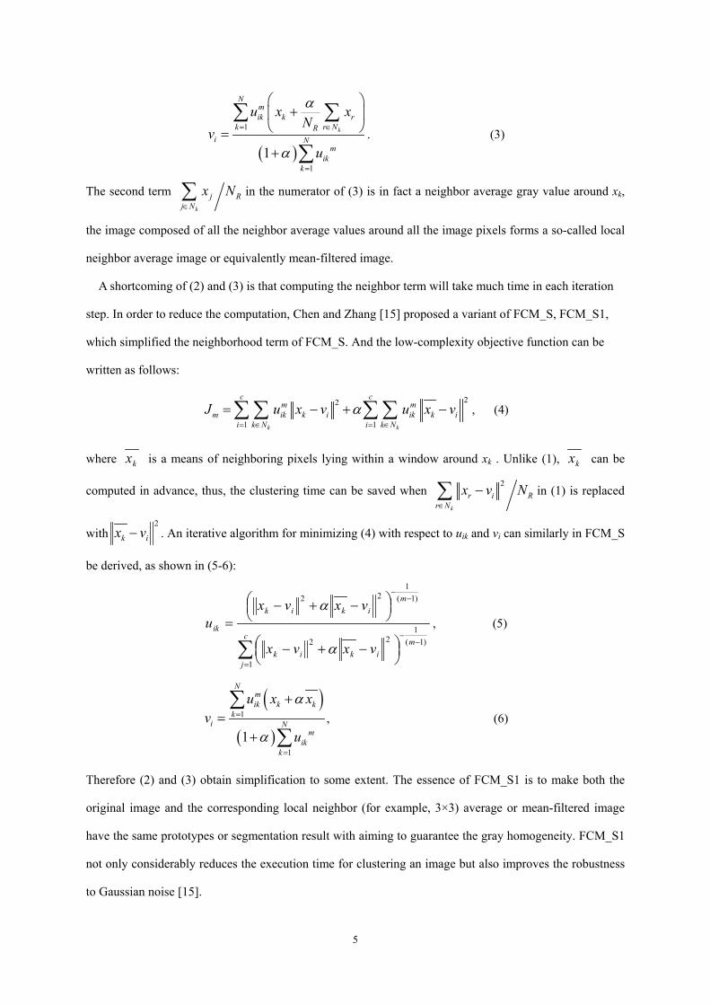
∑. (3)
The second term k
j Rj N
x N∈∑ in the numerator of (3) is in fact a neighbor average gray value around xk,
the image composed of all the neighbor average values around all the image pixels forms a so-called local
neighbor average image or equivalently mean-filtered image.
A shortcoming of (2) and (3) is that computing the neighbor term will take much time in each iteration
step. In order to reduce the computation, Chen and Zhang [15] proposed a variant of FCM_S, FCM_S1,
which simplified the neighborhood term of FCM_S. And the low-complexity objective function can be
written as follows:
22
1 1k k
c cm m
m ik k i ik k ii k N i k N
J u x v u x vα= ∈ = ∈
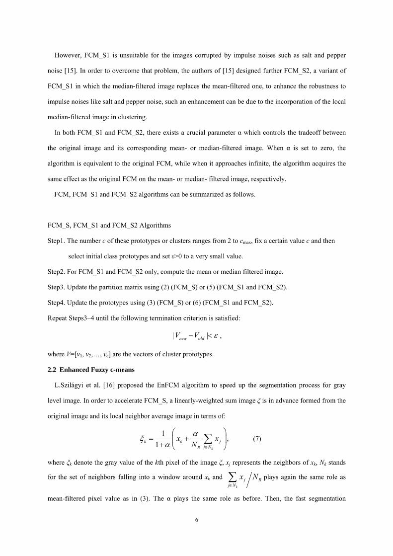
= − + −∑ ∑ ∑∑ , (4)
where kx is a means of neighboring pixels lying within a window around xk . Unlike (1), kx can be
computed in advance, thus, the clustering time can be saved when 2
k
r i Rr N
x v N∈
−∑ in (1) is replaced
with2
ik vx − . An iterative algorithm for minimizing (4) with respect to uik and vi can similarly in FCM_S
be derived, as shown in (5-6):
∑=
−−
−−
⎟⎠⎞⎜
⎝⎛ −+−
⎟⎠⎞⎜
⎝⎛ −+−
=c
j
mikik
mikik
ik
vxvx
vxvxu
1
)1(1
22
)1(1
22
α
α, (5)
( )( )1
1
1
Nmik k k
ki N
mik
k
u x xv
u
α
α
=
=
+=
+
∑
∑, (6)
Therefore (2) and (3) obtain simplification to some extent. The essence of FCM_S1 is to make both the
original image and the corresponding local neighbor (for example, 3×3) average or mean-filtered image
have the same prototypes or segmentation result with aiming to guarantee the gray homogeneity. FCM_S1
not only considerably reduces the execution time for clustering an image but also improves the robustness
to Gaussian noise [15].
6
However, FCM_S1 is unsuitable for the images corrupted by impulse noises such as salt and pepper
noise [15]. In order to overcome that problem, the authors of [15] designed further FCM_S2, a variant of
FCM_S1 in which the median-filtered image replaces the mean-filtered one, to enhance the robustness to
impulse noises like salt and pepper noise, such an enhancement can be due to the incorporation of the local
median-filtered image in clustering.
In both FCM_S1 and FCM_S2, there exists a crucial parameter α which controls the tradeoff between
the original image and its corresponding mean- or median-filtered image. When α is set to zero, the
algorithm is equivalent to the original FCM, while when it approaches infinite, the algorithm acquires the
same effect as the original FCM on the mean- or median- filtered image, respectively.
FCM, FCM_S1 and FCM_S2 algorithms can be summarized as follows.
FCM_S, FCM_S1 and FCM_S2 Algorithms
Step1. The number c of these prototypes or clusters ranges from 2 to cmax, fix a certain value c and then
select initial class prototypes and set ε>0 to a very small value.
Step2. For FCM_S1 and FCM_S2 only, compute the mean or median filtered image.
Step3. Update the partition matrix using (2) (FCM_S) or (5) (FCM_S1 and FCM_S2).
Step4. Update the prototypes using (3) (FCM_S) or (6) (FCM_S1 and FCM_S2).
Repeat Steps3–4 until the following termination criterion is satisfied:
| |new oldV V ε− < ,
where V=[v1, v2,…, vc] are the vectors of cluster prototypes.
2.2 Enhanced Fuzzy c-means
L.Szilágyi et al. [16] proposed the EnFCM algorithm to speed up the segmentation process for gray
level image. In order to accelerate FCM_S, a linearly-weighted sum image ξ is in advance formed from the
original image and its local neighbor average image in terms of:
11
k
k k jj NR
x xNαξ
α ∈
⎛ ⎞= +⎜ ⎟
+ ⎝ ⎠∑ , (7)
where ξk denote the gray value of the kth pixel of the image ξ, xj represents the neighbors of xk, Nk stands
for the set of neighbors falling into a window around xk and k
j Rj N
x N∈∑ plays again the same role as
mean-filtered pixel value as in (3). The α plays the same role as before. Then, the fast segmentation
7
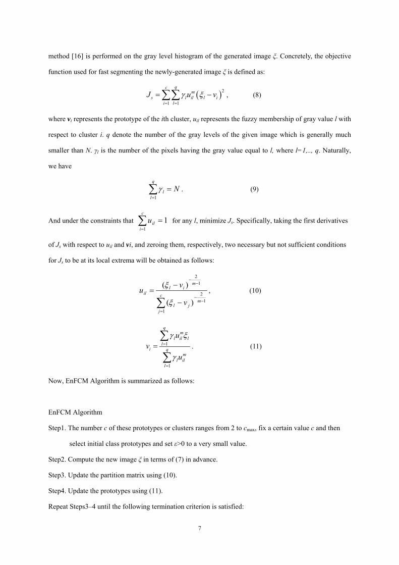
method [16] is performed on the gray level histogram of the generated image ξ. Concretely, the objective
function used for fast segmenting the newly-generated image ξ is defined as:
( )2
1 1
qcm
s l il l ii l
J u vγ ξ= =
= −∑∑ , (8)
where vi represents the prototype of the ith cluster, uil represents the fuzzy membership of gray value l with
respect to cluster i. q denote the number of the gray levels of the given image which is generally much
smaller than N. γl is the number of the pixels having the gray value equal to l, where l=1,.., q. Naturally,
we have
Nq
ll =∑
=1γ . (9)
And under the constraints that 11
=∑=
c
iilu for any l, minimize Js. Specifically, taking the first derivatives
of Js with respect to uil and vi, and zeroing them, respectively, two necessary but not sufficient conditions
for Js to be at its local extrema will be obtained as follows:
∑=
−−
−−
−
−=
c
j
mjl
mil
il
v
vu
1
12
12
)(
)(
ξ
ξ, (10)
1
1
qm
l il ll
i qm
l ill
uv
u
γ ξ
γ
=
=
=∑
∑. (11)
Now, EnFCM Algorithm is summarized as follows:
EnFCM Algorithm
Step1. The number c of these prototypes or clusters ranges from 2 to cmax, fix a certain value c and then
select initial class prototypes and set ε>0 to a very small value.
Step2. Compute the new image ξ in terms of (7) in advance.
Step3. Update the partition matrix using (10).
Step4. Update the prototypes using (11).
Repeat Steps3–4 until the following termination criterion is satisfied:
8
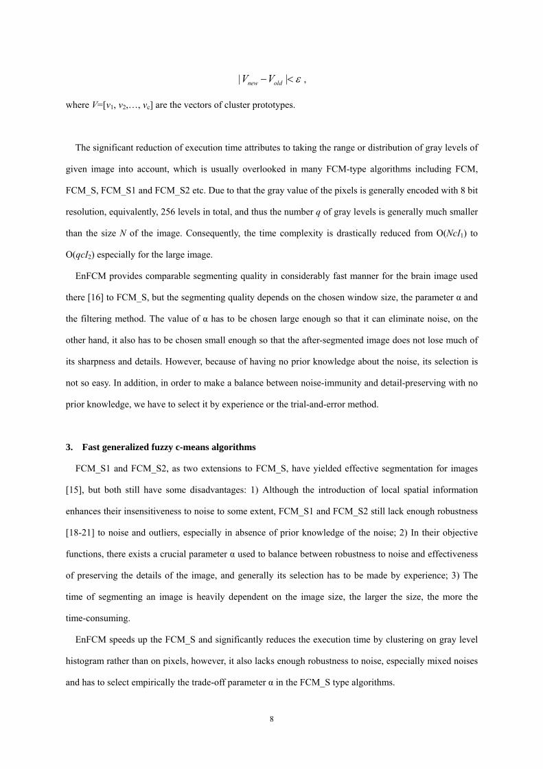
| |new oldV V ε− < ,
where V=[v1, v2,…, vc] are the vectors of cluster prototypes.
The significant reduction of execution time attributes to taking the range or distribution of gray levels of
given image into account, which is usually overlooked in many FCM-type algorithms including FCM,
FCM_S, FCM_S1 and FCM_S2 etc. Due to that the gray value of the pixels is generally encoded with 8 bit
resolution, equivalently, 256 levels in total, and thus the number q of gray levels is generally much smaller
than the size N of the image. Consequently, the time complexity is drastically reduced from O(NcI1) to
O(qcI2) especially for the large image.
EnFCM provides comparable segmenting quality in considerably fast manner for the brain image used
there [16] to FCM_S, but the segmenting quality depends on the chosen window size, the parameter α and
the filtering method. The value of α has to be chosen large enough so that it can eliminate noise, on the
other hand, it also has to be chosen small enough so that the after-segmented image does not lose much of
its sharpness and details. However, because of having no prior knowledge about the noise, its selection is
not so easy. In addition, in order to make a balance between noise-immunity and detail-preserving with no
prior knowledge, we have to select it by experience or the trial-and-error method.
3. Fast generalized fuzzy c-means algorithms
FCM_S1 and FCM_S2, as two extensions to FCM_S, have yielded effective segmentation for images
[15], but both still have some disadvantages: 1) Although the introduction of local spatial information
enhances their insensitiveness to noise to some extent, FCM_S1 and FCM_S2 still lack enough robustness
[18-21] to noise and outliers, especially in absence of prior knowledge of the noise; 2) In their objective
functions, there exists a crucial parameter α used to balance between robustness to noise and effectiveness
of preserving the details of the image, and generally its selection has to be made by experience; 3) The
time of segmenting an image is heavily dependent on the image size, the larger the size, the more the
time-consuming.
EnFCM speeds up the FCM_S and significantly reduces the execution time by clustering on gray level
histogram rather than on pixels, however, it also lacks enough robustness to noise, especially mixed noises
and has to select empirically the trade-off parameter α in the FCM_S type algorithms.
9
Motivated by individual strengths of FCM_S1, FCM_S2 and EnFCM, we propose a novel fast and
robust FCM framework for image segmentation in this paper called Fast Generalized Fuzzy c-means
clustering algorithms incorporating local information (FGFCM).
3.1 A novel local (spatial and gray) similarity measure Sij
FCM_S, FCM_S1, FCM_S2 and EnFCM all share a common parameter α and its selection is generally
important as well as difficult. The importance is due to that the parameter α must be adopted to make some
balance between robustness to noise and effectiveness of preserving the details for image. And the
difficulty of its selection results from such a fact that the determination of α is noise-dependent but the
types and intensity of the noise are generally a priori unknown and thus extensive trial-and-error
experiments has to be carried out, which significantly increases the computational burden. Even if the prior
knowledge of noise can be known, the adjustment for it also should follow such a rule of thumb [14] that
its value must be taken large enough for those pixels corrupted by relatively heavy noise, which will
unavoidably incur unnecessary blur for pixels not corrupted by the noise and thus lead to loss of some
details in image. On the other hand, its value should be small for those pixels with no and little noise
corruption. Therefore, setting the same value of α for all the neighbors of the pixels over the image during
segmentation or clustering is intuitively obviously unreasonable. In other words, the setting for α should
take into account: 1) the spatial or location relationship of pixels within the neighbor window, for example,
when the window size is expanded from 3×3 to 5×5, α should be set to different value for different spatial
distance from the center of the window, otherwise some blur is unavoidably introduced for given image; 2)
the gray level or intensity relationship of the pixels within the same window, such a relationship can reflect
the local neighborhood inhomogeneity of the window and thus setting the different values of α for different
pixels within the window can not only suppress the influence of the outlier but also avoid blur for given
image to some extent.
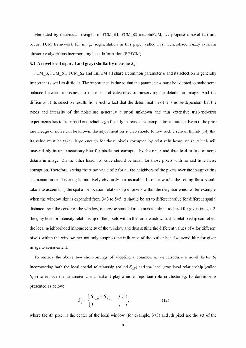
To remedy the above two shortcomings of adopting a common α, we introduce a novel factor Sij
incorporating both the local spatial relationship (called Ss_ij) and the local gray level relationship (called
Sg_ij) to replace the parameter α and make it play a more important role in clustering. Its definition is
presented as below:
⎩⎨⎧
=
≠×=
ij
ijSSS ijgijs
ij 0__ . (12)
where the ith pixel is the center of the local window (for example, 3×3) and jth pixel are the set of the

10
neighbors falling into a window around the ith pixel.
It is easy to see that the introduction of Ss_ij naturally overcomes the first limitation of using a common α
over an image in FCM_S etc. Ss_ij makes the influence of the pixels within the local window change
flexibly according to their distance from the central pixel and thus more local information can be used.
Here the definition of Ss_ij is given as follows:
( )_
max ,exp
j i j is ij
s
p p q qS
λ
⎛ ⎞− − −⎜ ⎟=⎜ ⎟⎝ ⎠
, (13)
where (pi , qi ) is a spatial coordinate of the ith pixel and we assume one pixel is one unit length in the
above computation. λs denotes the scale factor of the spread of Ss_ij, determining the change characteristic
of Ss_ij, thus its varying range is relatively easily determined. It is worth indicating that the shape of local
window defined here is square, however, the windows with other shapes such as diamond can also
naturally be adopted in our algorithm. As a whole, Ss_ij reflects the damping extent of the neighbors with
the spatial distances from the central pixel. In contrast, the parameter α in FCM_S, FCM_S1, FCM_S2 and
EnFCM is globally taken as a constant and thus it is relatively difficult to vary adaptively with different
spatial locations or distances from the central pixel. When λs are set to 1, 3 and 10 respectively, the
changing trend of Ss_ij against the size of the window are shown as below:
0 1 2 3 4 5 6 7 8 90
0.1
0.2
0.3
0.4
0.5
0.6
0.7
0.8
0.9
1
window size
Sspatial
λs=10
λs=3
λs=1
Fig. 1. Changing trend of S s_ij against the size of the window
From Fig. 1, we can see that for some λs , the nearer to the window center the location is, the larger the Ss_ij
value is, thus Ss_ij reflects different damping extent for pixels according to different spatial locations within
a given window.
In order to mitigate the second shortcoming resulting from the same parameter α, we define the local
gray level similarity measure Sg_ij as follows:
11
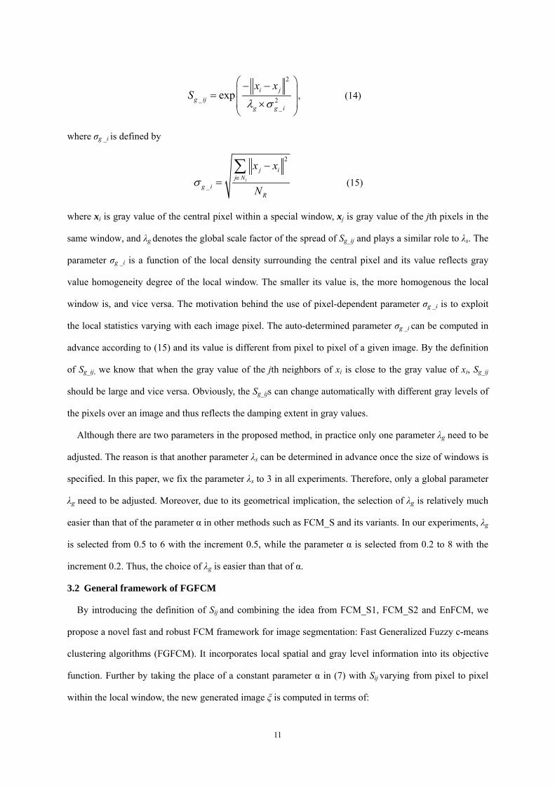
2
_ 2_
exp i jg ij
g g i
x xS
λ σ
⎛ ⎞− −⎜ ⎟=⎜ ⎟×⎝ ⎠
, (14)
where σg _i is defined by
2
_i
j ij N
g iR
x x
Nσ ∈
−=∑
(15)
where xi is gray value of the central pixel within a special window, xj is gray value of the jth pixels in the
same window, and λg denotes the global scale factor of the spread of Sg_ij and plays a similar role to λs. The
parameter σg _i is a function of the local density surrounding the central pixel and its value reflects gray
value homogeneity degree of the local window. The smaller its value is, the more homogenous the local
window is, and vice versa. The motivation behind the use of pixel-dependent parameter σg _i is to exploit
the local statistics varying with each image pixel. The auto-determined parameter σg _i can be computed in
advance according to (15) and its value is different from pixel to pixel of a given image. By the definition
of Sg_ij, we know that when the gray value of the jth neighbors of xi is close to the gray value of xi, Sg_ij
should be large and vice versa. Obviously, the Sg_ijs can change automatically with different gray levels of
the pixels over an image and thus reflects the damping extent in gray values.
Although there are two parameters in the proposed method, in practice only one parameter λg need to be
adjusted. The reason is that another parameter λs can be determined in advance once the size of windows is
specified. In this paper, we fix the parameter λs to 3 in all experiments. Therefore, only a global parameter
λg need to be adjusted. Moreover, due to its geometrical implication, the selection of λg is relatively much
easier than that of the parameter α in other methods such as FCM_S and its variants. In our experiments, λg
is selected from 0.5 to 6 with the increment 0.5, while the parameter α is selected from 0.2 to 8 with the
increment 0.2. Thus, the choice of λg is easier than that of α.
3.2 General framework of FGFCM
By introducing the definition of Sij and combining the idea from FCM_S1, FCM_S2 and EnFCM, we
propose a novel fast and robust FCM framework for image segmentation: Fast Generalized Fuzzy c-means
clustering algorithms (FGFCM). It incorporates local spatial and gray level information into its objective
function. Further by taking the place of a constant parameter α in (7) with Sij varying from pixel to pixel
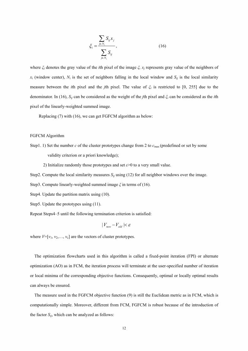
within the local window, the new generated image ξ is computed in terms of:
12
i
i
ij jj N
i
ijj N
S x
Sξ ∈
∈
=∑
∑, (16)
where ξi denotes the gray value of the ith pixel of the image ξ, xj represents gray value of the neighbors of
xi (window center), Ni is the set of neighbors falling in the local window and Sij is the local similarity
measure between the ith pixel and the jth pixel. The value of ξi is restricted to [0, 255] due to the
denominator. In (16), Sij can be considered as the weight of the jth pixel and ξi can be considered as the ith
pixel of the linearly-weighted summed image.
Replacing (7) with (16), we can get FGFCM algorithm as below:
FGFCM Algorithm
Step1. 1) Set the number c of the cluster prototypes change from 2 to cmax (predefined or set by some
validity criterion or a priori knowledge);
2) Initialize randomly those prototypes and set ε>0 to a very small value.
Step2. Compute the local similarity measures Sij using (12) for all neighbor windows over the image.
Step3. Compute linearly-weighted summed image ξ in terms of (16).
Step4. Update the partition matrix using (10).
Step5. Update the prototypes using (11).
Repeat Steps4–5 until the following termination criterion is satisfied:
| |new oldV V ε− <
where V=[v1, v2,…, vc] are the vectors of cluster prototypes.
The optimization flowcharts used in this algorithm is called a fixed-point iteration (FPI) or alternate
optimization (AO) as in FCM, the iteration process will terminate at the user-specified number of iteration
or local minima of the corresponding objective functions. Consequently, optimal or locally optimal results
can always be ensured.
The measure used in the FGFCM objective function (9) is still the Euclidean metric as in FCM, which is
computationally simple. Moreover, different from FCM, FGFCM is robust because of the introduction of
the factor Sij, which can be analyzed as follows:
13
Seen from (16), the noise tolerance and outliers resistance property of ξi completely relies on the
definition of Sij. In the absence of prior knowledge of the noise, Sij should automatically be determined
rather than artificially set. Especially, the Sij of the noise-corrupted pixels within a window should keep
small and thus the influence of noise can be ignored. The Sij used in FGFCM can be adaptively changed
and thus guarantee the insensitive to noise and outliers. The presence of the noise and outliers can
generally be divided into two cases below:
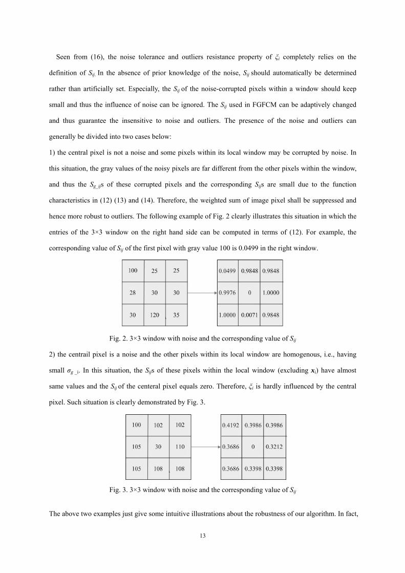
1) the central pixel is not a noise and some pixels within its local window may be corrupted by noise. In
this situation, the gray values of the noisy pixels are far different from the other pixels within the window,
and thus the Sg_ijs of these corrupted pixels and the corresponding Sijs are small due to the function
characteristics in (12) (13) and (14). Therefore, the weighted sum of image pixel shall be suppressed and
hence more robust to outliers. The following example of Fig. 2 clearly illustrates this situation in which the
entries of the 3×3 window on the right hand side can be computed in terms of (12). For example, the
corresponding value of Sij of the first pixel with gray value 100 is 0.0499 in the right window.
Fig. 2. 3×3 window with noise and the corresponding value of Sij
2) the centrail pixel is a noise and the other pixels within its local window are homogenous, i.e., having
small σg _i. In this situation, the Sijs of these pixels within the local window (excluding xi) have almost
same values and the Sij of the centeral pixel equals zero. Therefore, ξi is hardly influenced by the central
pixel. Such situation is clearly demonstrated by Fig. 3.
Fig. 3. 3×3 window with noise and the corresponding value of Sij
The above two examples just give some intuitive illustrations about the robustness of our algorithm. In fact,
14
their theoretical ground can also be verified from the viewpoint of robustified filters [22-23] and
locality-based methods [24]. Concretely, according to the robust filtering viewpoint, the reformulation of
(16) is similar to the filtered result derived by optimizing a kernel-induced robust measure [25-26] based
on classical linear mean filter. On the other hand according to the locality-based methods, the incorporation
of the Sij with spatial and gray localities to (16) can also enhance its robustness to noise and outliers. Due
to the space limit, we omitted the details of the proof here.
It is also worth to point out that the denoising method used in FGFCM is different from the one used in
FCM_S1 and FCM_S2. FCM_S1 is relatively suitable for the noisy image corrupted by Gaussian noise
due to using a mean-type filtering, while FCM_S2 is relatively suitable for the image corrupted by impulse
noises like salt and pepper noise due to use of a median-type filtering. And the final effectiveness of
removing the noise in clustering relies on the value of the parameter α. Without the prior knowledge of the
noise, it is generally hard to choose the proper one between FCM_S1 and FCM_S2 and the optimal value
of α for image segmentation. Compared with FCM_S1 or _S2, the denoising method in FGFCM is
independent of the type of noise and its effectiveness seems insensitive to the spatial scale factor λs and the
gray level scale factor λg to some extent as shown in the experiments later.
Sij not only guarantees the robustness to noise and outliers but also seems to preserve more image
information. It incorporates both local spatial relationship Ss_ij which changes adaptively according to
spatial distances from the central pixel, and the local gray level relationship Sg_ij which varies
automatically according to different gray level difference between the pixels over an image. Thus, the
value of Sij varies from pixel to pixel within a neighbor window, which likely preserves more information
than using same value for each pixel. Therefore, FGFCM adopting Sij seems able to perserve more image
details than EnFCM.
In the following, major characteristics of FGFCM are summarized:
(1) using a new factor Sij as a local (spatial and gray) similarity measure with aiming to guarantee both
noise-immunity and detail-preserving for image, and at the same time remove the empirically-adjusted
parameter α;
(2) fast clustering or segmentation for given image, the segmenting time is only dependent on the number
of the gray levels q rather than the size N (>>q) of the image, and consequently its computational
complexity is reduced from O(NcI1) to O(qcI2),
15
3.3 Relationship between FGFCM and other methods
Fast generalized fuzzy c-means clustering algorithms can be considered as a general framework. In fact,
the structure of the framework FGFCM can be decomposed into the following two steps. In the first step, a
linearly-weighted sum image ξ is generated according to different definition of Sij, and in the second step,
the fast segmentation method [16] is performed on the gray level histogram of the generated image ξ.
Besides FGFCM, some other typical clustering algorithms for image segmentation can be derived from
the framework according to different definition of Sij as follows:
1) By directly setting Sij in (16) in terms of
⎩⎨⎧
≠=
=ijij
Sij 01
, (17)
FGFCM algorithm reduces into fast versions of the standard FCM, which is a special case of FGFCM.
2) By directly setting Sij in (16) in terms of
1Rij
j iNS
j i
α⎧ ≠⎪= ⎨⎪ =⎩
, (18)
FGFCM algorithm reduces into EnFCM, that is, the latter is a special case of FGFCM algorithm.
3) Motivated by FCM_S1, Sij in (16) is defined as
1ijS = , for all i and j (19)
and naturally ξi equals to the mean of the neighbors within a specified window including the ith pixel. And
this algorithm derived from FGFCM framework is called FGFCM_S1.
4) Motivated by FCM_S2, Sij in (16) is defined as
( )1
0
jjij
j j j median xS
j j
∗ ∗
∗
⎧ = =⎪= ⎨⎪ ≠⎩
, (20)
and consequently ζi equals to the median of the neighbors within a specified window including the ith pixel.
And this algorithm is named FGFCM_S2 under the framework of FGFCM.
4. Experiment Results
In this section, we compare the effectiveness and efficiency of six algorithms FCM_S1, FCM_S2,
EnFCM, FGFCM_S1, FGFCM_S2 and FGFCM on some synthetic and real images. In all the following
experiments, we set the parameters λs=3, ε=0.00001 and NR=8 (a 3×3 window centered around each pixel,
16
except the central pixel itself).
In our experiments, we use the images corrupted respectively by the Gaussian noise and salt and pepper
noise to test the robustness of the algorithms. Besides the above two types of noises, we also use the
images with the mixed noise for more practical applications, this mixed noise is not simply pure Gaussian
or impulsive noise but mixture of both whose distribution obeys Pη=(1-η)G+ηS where G denotes the
Gaussian with zero mean and variance of σ2G and S the SαS (Symmetric α-Stable, here abuse parameter α)
with location θ and dispersion γs and thus the characteristic function φ(t) [27-28] of Pη can be formulated as
( ) 2 2exp (1 ) [0,1]2G
St j t t t αασϕ ηθ η η γ η⎛ ⎞= − − − ∈⎜ ⎟⎝ ⎠
, (21)
where the parameter α controls how impulsive the distribution is. The η used in the following experiment
is set to 2/ (2+π) [28].
4.1 Results on synthetic image
To compare the denoising performances of the above six algorithms, we apply these algorithms to a
synthetic test image as shown in Fig. 4(a) (128×128 pixels, two classes with two gray values taken as 0 and
90) corrupted by different levels of Gaussian noise, salt and pepper noise and mixed noise, respectively.
The mixed noise used in this experiment is the mixture of Gaussian white noise N (0,100) and unit
dispersion, zero centered symmetric α-stable (SαS) noise. The parameters used in each noisy image are c=2
and λg=6. And at the same time, αs in the algorithms of FCM_S1, FCM_S2 and EnFCM are all chosen as
3.8 [15] which is obtained by searching the interval [0.2, 8] with respect to the optimal segmentation
accuracy (SA), where SA is defined as the sum of the total number of pixels divided by the sum of number
of correctly classified pixels [14].
4.1.1 Comparison of segmentation results on synthetic image corrupted by mixed noise
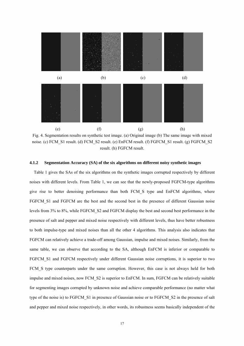
Figs. 4 are the segmenting results on a corrupted image with mixed noise (α=0.7 in SαS). FCM_S1, _S2
and EnFCM are respectively affected by the noise to different extents which indicates that these algorithms
lack enough robustness to the mixed noise. Visually, FGFCM_S1 removes most of the noise, FGFCM_S2
and FGFCM algorithms achieve relatively satisfactory results. More detailed quantified comparisons
according to segmentation accuracy (SA) on different noise levels are given the next subsection.
17
(a) (b) (c) (d)
(e) (f) (g) (h) Fig. 4. Segmentation results on synthetic test image. (a) Original image (b) The same image with mixed noise. (c) FCM_S1 result. (d) FCM_S2 result. (e) EnFCM result. (f) FGFCM_S1 result. (g) FGFCM_S2
result. (h) FGFCM result.
4.1.2 Segmentation Accuracy (SA) of the six algorithms on different noisy synthetic images
Table 1 gives the SAs of the six algorithms on the synthetic images corrupted respectively by different
noises with different levels. From Table 1, we can see that the newly-proposed FGFCM-type algorithms
give rise to better denoising performance than both FCM_S type and EnFCM algorithms, where
FGFCM_S1 and FGFCM are the best and the second best in the presence of different Gaussian noise
levels from 3% to 8%, while FGFCM_S2 and FGFCM display the best and second best performance in the
presence of salt and pepper and mixed noise respectively with different levels, thus have better robustness
to both impulse-type and mixed noises than all the other 4 algorithms. This analysis also indicates that
FGFCM can relatively achieve a trade-off among Gaussian, impulse and mixed noises. Similarly, from the
same table, we can observe that according to the SA, although EnFCM is inferior or comparable to
FGFCM_S1 and FGFCM respectively under different Gaussian noise corruptions, it is superior to two
FCM_S type counterparts under the same corruption. However, this case is not always held for both
impulse and mixed noises, now FCM_S2 is superior to EnFCM. In sum, FGFCM can be relatively suitable
for segmenting images corrupted by unknown noise and achieve comparable performance (no matter what
type of the noise is) to FGFCM_S1 in presence of Gaussian noise or to FGFCM_S2 in the presence of salt
and pepper and mixed noise respectively, in other words, its robustness seems basically independent of the
18
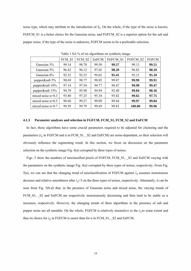
noise type, which may attribute to the introduction of Sij. On the whole, if the type of the noise is known,
FGFCM_S1 is a better choice for the Gaussian noise, and FGFCM_S2 is a superior option for the salt and
pepper noise; if the type of the noise is unknown, FGFCM seems to be a preferable selection.
Table 1 SA % of six algorithms on synthetic image
FCM_S1 FCM_S2 EnFCM FGFCM_S1 FGFCM_S2 FGFCMGaussian 3% 99.14 98.78 99.50 99.57 99.13 99.51 Gaussian 5% 96.42 96.12 97.65 98.20 96.82 98.10 Gaussian 8% 92.32 92.23 94.62 95.41 93.12 95.10
pepper&salt 5% 98.69 98.77 98.05 99.07 99.99 99.91 pepper&salt 10% 97.14 97.54 94.77 96.47 99.98 99.47 pepper&salt 15% 94.78 95.98 94.94 92.40 99.84 98.36 mixed noise α=0.3 93.80 97.25 95.34 95.82 99.65 97.75 mixed noise α=0.5 98.68 99.27 99.09 99.44 99.97 99.84 mixed noise α=0.7 99.59 99.79 99.69 99.83 100.00 99.96
4.1.3 Parameter analyses and selection in FGFCM, FCM_S1, FCM_S2 and EnFCM
In fact, those algorithms have some crucial parameters required to be adjusted for clustering and the
parameters (λg in FGFCM and α in FCM_S1, _S2 and EnFCM) are noise-dependent, so their selection will
obviously influence the segmenting result. In this section, we focus on discussion on the parameter
selection on the synthetic image Fig. 4(a) corrupted by three types of noises.
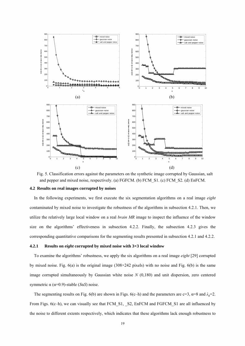
Figs. 5 show the numbers of misclassified pixels of FGFCM, FCM_S1, _S2 and EnFCM varying with
the parameters on the synthetic image Fig. 4(a) corrupted by three types of noises, respectively. From Fig.
5(a), we can see that the changing trend of misclassification of FGFCM against λg assumes monotonous
decrease and relative smoothness after λg=3 on the three types of noises, respectively. Alternately, it can be
seen from Fig. 5(b-d) that, in the presence of Gaussian noise and mixed noise, the varying trends of
FCM_S1, _S2 and EnFCM are respectively monotonously decreasing and then tend to be stable as α
increases, respectively. However, the changing trends of three algorithms in the presence of salt and
pepper noise are all unstable. On the whole, FGFCM is relatively insensitive to the λg to some extent and
thus its choice for λg in FGFCM is easier than for α in FCM_S1, _S2 and EnFCM.
19
0 1 2 3 4 5 6
0
100
200
300
400
500
600
700
800
900
λg
number of misclassified pixels
mixed noisegaussian noisesalt and pepper noise
0 1 2 3 4 5 6 7 8 9 100
100
200
300
400
500
600
700
800
900
α
number of misclassified pixels
mixed noisegaussian noisesalt and pepper noise
(a) (b)
0 1 2 3 4 5 6 7 8 9 100
100
200
300
400
500
600
700
800
900
α
number of misclassified pixels
mixed noisegaussian noisesalt and pepper noise
0 1 2 3 4 5 6 7 8 9 100
100
200
300
400
500
600
700
800
900
α
number of misclassified pixels
mixed noisegaussian noisesalt and pepper noise
(c) (d)
Fig. 5. Classification errors against the parameters on the synthetic image corrupted by Gaussian, salt and pepper and mixed noise, respectively. (a) FGFCM. (b) FCM_S1. (c) FCM_S2. (d) EnFCM.
4.2 Results on real images corrupted by noises
In the following experiments, we first execute the six segmentation algorithms on a real image eight
contaminated by mixed noise to investigate the robustness of the algorithms in subsection 4.2.1. Then, we
utilize the relatively large local window on a real brain MR image to inspect the influence of the window
size on the algorithms’ effectiveness in subsection 4.2.2. Finally, the subsection 4.2.3 gives the
corresponding quantitative comparisons for the segmenting results presented in subsection 4.2.1 and 4.2.2.
4.2.1 Results on eight corrupted by mixed noise with 3×3 local window
To examine the algorithms’ robustness, we apply the six algorithms on a real image eight [29] corrupted
by mixed noise. Fig. 6(a) is the original image (308×242 pixels) with no noise and Fig. 6(b) is the same
image corrupted simultaneously by Gaussian white noise N (0,180) and unit dispersion, zero centered
symmetric α (α=0.9)-stable (SαS) noise.
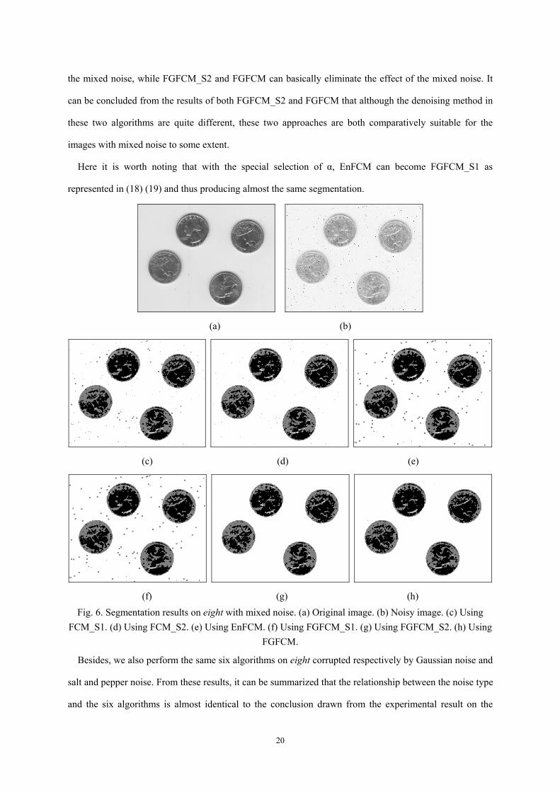
The segmenting results on Fig. 6(b) are shown in Figs. 6(c–h) and the parameters are c=3, α=8 and λg=2.
From Figs. 6(c–h), we can visually see that FCM_S1, _S2, EnFCM and FGFCM_S1 are all influenced by
the noise to different extents respectively, which indicates that these algorithms lack enough robustness to
20
the mixed noise, while FGFCM_S2 and FGFCM can basically eliminate the effect of the mixed noise. It
can be concluded from the results of both FGFCM_S2 and FGFCM that although the denoising method in
these two algorithms are quite different, these two approaches are both comparatively suitable for the
images with mixed noise to some extent.
Here it is worth noting that with the special selection of α, EnFCM can become FGFCM_S1 as
represented in (18) (19) and thus producing almost the same segmentation.
(a) (b)
(c) (d) (e)
(f) (g) (h) Fig. 6. Segmentation results on eight with mixed noise. (a) Original image. (b) Noisy image. (c) Using
FCM_S1. (d) Using FCM_S2. (e) Using EnFCM. (f) Using FGFCM_S1. (g) Using FGFCM_S2. (h) Using FGFCM.
Besides, we also perform the same six algorithms on eight corrupted respectively by Gaussian noise and
salt and pepper noise. From these results, it can be summarized that the relationship between the noise type
and the six algorithms is almost identical to the conclusion drawn from the experimental result on the
21
synthetic image in subsection 4.1 and also consistent with the theoretical analysis about FGFCM in
subsection 3.2.
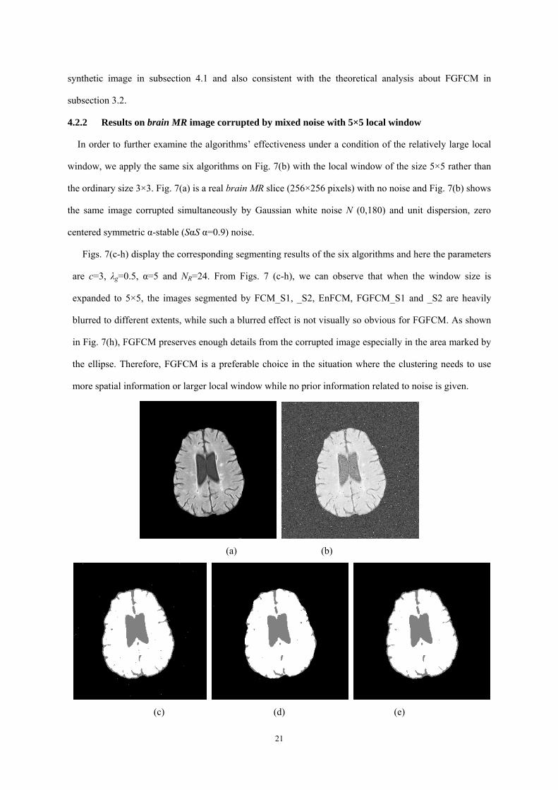
4.2.2 Results on brain MR image corrupted by mixed noise with 5×5 local window
In order to further examine the algorithms’ effectiveness under a condition of the relatively large local
window, we apply the same six algorithms on Fig. 7(b) with the local window of the size 5×5 rather than
the ordinary size 3×3. Fig. 7(a) is a real brain MR slice (256×256 pixels) with no noise and Fig. 7(b) shows
the same image corrupted simultaneously by Gaussian white noise N (0,180) and unit dispersion, zero
centered symmetric α-stable (SαS α=0.9) noise.
Figs. 7(c-h) display the corresponding segmenting results of the six algorithms and here the parameters
are c=3, λg=0.5, α=5 and NR=24. From Figs. 7 (c-h), we can observe that when the window size is
expanded to 5×5, the images segmented by FCM_S1, _S2, EnFCM, FGFCM_S1 and _S2 are heavily
blurred to different extents, while such a blurred effect is not visually so obvious for FGFCM. As shown
in Fig. 7(h), FGFCM preserves enough details from the corrupted image especially in the area marked by
the ellipse. Therefore, FGFCM is a preferable choice in the situation where the clustering needs to use
more spatial information or larger local window while no prior information related to noise is given.
(a) (b)
(c) (d) (e)
22
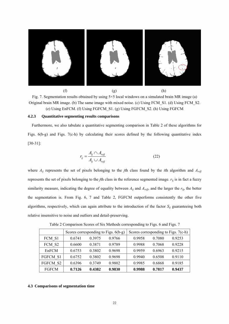
(f) (g) (h)
Fig. 7. Segmentation results obtained by using 5×5 local windows on a simulated brain MR image (a) Original brain MR image. (b) The same image with mixed noise. (c) Using FCM_S1. (d) Using FCM_S2.
(e) Using EnFCM. (f) Using FGFCM_S1. (g) Using FGFCM_S2. (h) Using FGFCM
4.2.3 Quantitative segmenting results comparisons
Furthermore, we also tabulate a quantitative segmenting comparison in Table 2 of these algorithms for
Figs. 6(b-g) and Figs. 7(c-h) by calculating their scores defined by the following quantitative index
[30-31]:
ij refjij
ij refj
A Ar
A A∩
=∪
(22)
where Aij represents the set of pixels belonging to the jth class found by the ith algorithm and Arefj
represents the set of pixels belonging to the jth class in the reference segmented image. rij is in fact a fuzzy
similarity measure, indicating the degree of equality between Aij and Arefj, and the larger the rij, the better
the segmentation is. From Fig. 6, 7 and Table 2, FGFCM outperforms consistently the other five
algorithms, respectively, which can again attribute to the introduction of the factor Sij guaranteeing both
relative insensitive to noise and outliers and detail-preserving.
Table 2 Comparison Scores of Six Methods corresponding to Figs. 6 and Figs. 7
Scores corresponding to Figs. 6(b-g) Scores corresponding to Figs. 7(c-h) FCM_S1 0.6741 0.3975 0.9766 0.9958 0.7080 0.9253 FCM_S2 0.6600 0.3871 0.9789 0.9988 0.7068 0.9228 EnFCM 0.6753 0.3802 0.9698 0.9959 0.6963 0.9215
FGFCM_S1 0.6752 0.3802 0.9698 0.9940 0.6508 0.9110 FGFCM_S2 0.6396 0.3749 0.9802 0.9985 0.6868 0.9185
FGFCM 0.7126 0.4382 0.9830 0.9988 0.7817 0.9437
4.3 Comparisons of segmentation time
23
In the subsection 3, we have theoretically analyzed the computational complexity of the second step in
the FGFCM framework and the goal of this subsection is to further experimentally investigate its practical
acceleration for image segmentation relative to standard FCM (FCM for short). Here we apply the fast
segmentation and FCM method on the after-filtered images ξ-1, ξ-2, ξ-3 and ξ-4. Concretely, ξ-1, ξ-2, ξ-3
and ξ-4 are generated on Fig. 8(a) according to (16) with respect to the four definitions of Sij in (18) (19)
(20) (12), respectively and the corresponding parameters are c=8, α=0.8 in (18) and λg=1 in (12),
respectively.
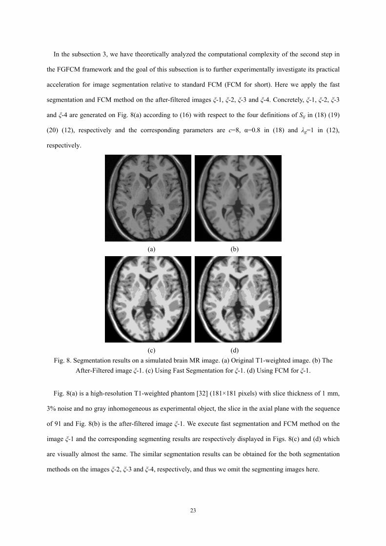
(a) (b)
(c) (d)
Fig. 8. Segmentation results on a simulated brain MR image. (a) Original T1-weighted image. (b) The After-Filtered image ξ-1. (c) Using Fast Segmentation for ξ-1. (d) Using FCM for ξ-1.
Fig. 8(a) is a high-resolution T1-weighted phantom [32] (181×181 pixels) with slice thickness of 1 mm,
3% noise and no gray inhomogeneous as experimental object, the slice in the axial plane with the sequence
of 91 and Fig. 8(b) is the after-filtered image ξ-1. We execute fast segmentation and FCM method on the
image ξ-1 and the corresponding segmenting results are respectively displayed in Figs. 8(c) and (d) which
are visually almost the same. The similar segmentation results can be obtained for the both segmentation
methods on the images ξ-2, ξ-3 and ξ-4, respectively, and thus we omit the segmenting images here.
24
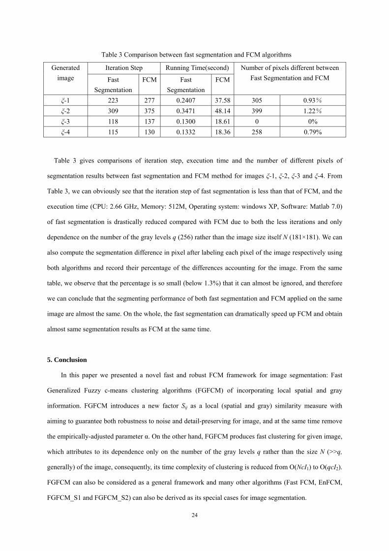
Table 3 Comparison between fast segmentation and FCM algorithms
Iteration Step Running Time(second)Generated image Fast
Segmentation FCM Fast
Segmentation FCM
Number of pixels different between Fast Segmentation and FCM
ξ-1 223 277 0.2407 37.58 305 0.93% ξ-2 309 375 0.3471 48.14 399 1.22% ξ-3 118 137 0.1300 18.61 0 0% ξ-4 115 130 0.1332 18.36 258 0.79%
Table 3 gives comparisons of iteration step, execution time and the number of different pixels of
segmentation results between fast segmentation and FCM method for images ξ-1, ξ-2, ξ-3 and ξ-4. From
Table 3, we can obviously see that the iteration step of fast segmentation is less than that of FCM, and the
execution time (CPU: 2.66 GHz, Memory: 512M, Operating system: windows XP, Software: Matlab 7.0)
of fast segmentation is drastically reduced compared with FCM due to both the less iterations and only
dependence on the number of the gray levels q (256) rather than the image size itself N (181×181). We can
also compute the segmentation difference in pixel after labeling each pixel of the image respectively using
both algorithms and record their percentage of the differences accounting for the image. From the same
table, we observe that the percentage is so small (below 1.3%) that it can almost be ignored, and therefore
we can conclude that the segmenting performance of both fast segmentation and FCM applied on the same
image are almost the same. On the whole, the fast segmentation can dramatically speed up FCM and obtain
almost same segmentation results as FCM at the same time.
5. Conclusion
In this paper we presented a novel fast and robust FCM framework for image segmentation: Fast
Generalized Fuzzy c-means clustering algorithms (FGFCM) of incorporating local spatial and gray
information. FGFCM introduces a new factor Sij as a local (spatial and gray) similarity measure with
aiming to guarantee both robustness to noise and detail-preserving for image, and at the same time remove
the empirically-adjusted parameter α. On the other hand, FGFCM produces fast clustering for given image,
which attributes to its dependence only on the number of the gray levels q rather than the size N (>>q,
generally) of the image, consequently, its time complexity of clustering is reduced from O(NcI1) to O(qcI2).
FGFCM can also be considered as a general framework and many other algorithms (Fast FCM, EnFCM,
FGFCM_S1 and FGFCM_S2) can also be derived as its special cases for image segmentation.
25
The results reported in this paper show that our proposed algorithm is general, simple and appropriate
for the images with various types of noises and the images with no noise. On the other hand, it is fast and
thus suitable for large-sized gray images.
Fast clustering method used in FGFCM seems to be able to be straightforwardly extended to the
segmenting algorithms for color images. However a problem will arise, i.e., the combination of the three
color values achieves 224 for a 24-bit RGB image, which is generally larger than the number of image
pixels. Therefore special preprocessing of the color image should be done before segmenting the given
color image.
Within the framework of FGFCM, the mean-LogCauchy (MLC) filter [28] can be incorporated to
promote the clustering performs in present of mixed noise. MLC, a convex combination of the mean and
the LogCauchy filters, has experimentally been proven capable to achieve best performance in removing
the mixed noise.
Our ongoing and further works include clustering validity in our algorithms, adaptive determination for
the clustering number and other applications, e.g., gain field estimation.
Acknowledgements
The authors would like to thank the anonymous referees for their helpful comments and suggestions to
improve the presentation of this paper. This work was supported by the National Science Foundation of
China under Grant No. 60505004, BK2006521 Jiangsu Postdoctoral Science Foundation and the Jiangsu
Science Foundation Key Project under Grant No. BK2004001.
References
[1] J.C. Bezdek, L.O. Hall, L.P. Clarke, Review of MR image segmentation techniques using pattern
recognition, Med. Phys., 20 (1993) 1033–1048.
[2] D.L. Pham, C.Y. Xu, J.L. Prince, A survey of current methods in medical image segmentation, Annu.
Rev. Biomed. Eng., 2 (2000) 315–337.
[3] W.M. Wells, W.E. LGrimson, R. Kikinis, S.R. Arrdrige, Adative segmentation of MRI data, IEEE
Trans. Med. Imag., 15 (1996) 429–442.
[4] J.C. Bezdek, Pattern Recognition With Fuzzy Objective Function Algorithms. New York: Plenum,
1981.
[5] J.K. Udupa, S. Samarasekera, Fuzzy connectedness and object definition: theory, algorithm and
26
applications in image segmentation, Graph. Models Image Process, 58(3) (1996) 246–261.
[6] S.M. Yamany, A.A. Farag, S. Hsu, A fuzzy hyperspectral classifier for automatic target recognition
(ATR) systems, Pattern Recognit. Lett., 20 (1999)1431–1438.
[7] M. S. Yang, Y. J. Hu, Karen, C. R. Lin and C. C. Lin,Segmentation techniques for tissue
differentiation in MRI of Ophthalmology using fuzzy clustering algorithms, Magnetic Resonance
Imaging,20 (2) (2002) 173-179
[8] G. C. Karmakar and L. S. Dooley, A generic fuzzy rule based image segmentation algorithm, Pattern
Recognition Letters, 23(10) (2002) 1215-1227
[9] D.L. Pham, J.L. Prince, An adaptive fuzzy C-means algorithm for image segmentation in the presence
of intensity inhomogeneities, Pattern Recognit. Lett., 20 (1999) 57–68.
[10] Y.A. Tolias and S.M. Panas, On applying spatial constraints in fuzzy image clustering using a fuzzy
rule-based system, IEEE Signal Processing Lett., 5 (1998) 245–247.
[11] Y.A. Tolias and S.M. Panas, Image segmentation by a fuzzy clustering algorithm using adaptive
spatially constrained membership functions, IEEE Trans. Syst.,Man, Cybern. A., 28 (1998) 359–369.
[12] A.W.C. Liew, S.H. Leung, W.H. Lau, Fuzzy image clustering incorporating spatial continuity, Inst.
Elec. Eng. Vis. Image Signal Process., 147 (2000) 185–192.
[13] D.L. Pham, Fuzzy clustering with spatial constraints, in IEEE Proc.Int. Conf. Image Processing, New
York, (2002) II-65–II-68.
[14] M.N. Ahmed, S.M. Yamany, N. Mohamed, A.A. Farag, T. Moriarty, A modified fuzzy C-means
algorithm for bias field estimation and segmentation of MRI data, IEEE Trans. Med. Imaging.,
21(2002) 193–199.
[15] S.C. Chen and D.Q. Zhang, Robust Image Segmentation Using FCM With Spatial Constraints Based
on New Kernel-Induced Distance Measure, IEEE Trans. Syst.,Man, Cybern. B., 34(4) (2004)
1907-1916
[16] L. Szilágyi, Z. Benyó, S.M. Szilágyii, H.S. Adam, MR Brain Image Segmentation Using an Enhanced
Fuzzy C-Means Algorithm, in 25th Annual International Conference of IEEE EMBS (2003)17-21.
[17] M. N. Ahmed, S.M. Yamany, N.A. Mohamed, A.A. Farag, T. Moriarty, Bias field estimation and
adaptive segmentation of MRI data using modified fuzzy C-means algorithm, in Proc. IEEE Int. Conf.
ComputerVision and Pattern Recogn., 1 (1999) 250–255.
[18] J. Leski, Toward a robust fuzzy clustering, Fuzzy Sets Syst., 137(2) (2003) 215–233.
27
[19] R.J. Hathaway, J.C. Bezdek, Generalized fuzzy c-means clustering strategies using L norm distance,
IEEE Trans. Fuzzy Syst., 8 (2000) 576–572.
[20] K. Jajuga, L norm based fuzzy clustering, Fuzzy Sets Syst., 39(1) (1991) 43–50.
[21] K.L. Wu, M.S. Yang, Alternative c-means clustering algorithms, Pattern Recognit., 35(2002)
2267–2278.
[22] K.R. Tan,, S.C. Chen, Robust Image Denoising Using Kernel-Induced Measures, Proceedings of the
17th International Conference on Pattern Recognition, Cambridge, United Kingdom (2004).
[23] P.J. Huber, Robust Statistics. New York: Wiley, 1981.
[24] X. He, P. Niyogi, Locality Preserving Projections, Advances in Neural Information Processing
Systems 16, MIT Press (2003).
[25] D.Q. Zhang, S.C. Chen, A novel kernelised fuzzy c-means algorithm with application in medical
image segmentation, Artificial Intelligence in Medicine., 32 (1) (2004) 37-50
[26] M. S. Yang, K. L. Wu, A similarity-based robust clustering method, IEEE T. PAMI., 26(4) (2004)
434-447
[27] E.E. Kuruoglu. C. Molina, S.J. Gosdill, W.J. Fitzgerald, A new analytic representation of the α-stable
density function, in Proc. Amer. Stat. Soc., (1997).
[28] A. Ben Hamza, H. Krim, Image denoising: A nonlinear robust statistical approach, IEEE Trans,
Signal processing, 49(12) (2001) 3045- 3053
[29] Mathworks, Natick, MA. Image Processing Toolbox. [Online] Available:htttp://www.mathworks.com
[30] C.T. Lin, C. S. G. Lee, Real-time supervised structure/parameter learning for fuzzy neural network,
Proceedings of the 1992 IEEE International Conference on Fuzzy Systems, San Diego, CA,
1283-1290.
[31] F. Masulli, A. Schenone, A fuzzy clustering based segmentation system as support to diagnosis in
medical imaging. Artif. Intell. Med. 16(2) (1999)129-147.
[32] R.K.S. Kwan, A.C. Evans, G.B. Pike, An extensible MRI simulator for post-processing evaluation,
Visualization in Biomedical Computing, Lecture Notes in Computer Science., 1131 (1996)135–140.