Embed Size (px)
Citation preview

Journal of Machine Learning Research 11 (2010) 1883-1926 Submitted 1/10; Published 6/10
Fast and Scalable Local Kernel Machines
Nicola Segata [email protected] .ITEnrico Blanzieri [email protected] .ITDepartment of Information Engineering and Computer ScienceUniversity of TrentoTrento, Italy
Editor: Leon Bottou
AbstractA computationally efficient approach to local learning withkernel methods is presented. TheFastLocalKernelSupportVectorMachine (FaLK-SVM) trains a set of local SVMs on redundant neigh-bourhoods in the training set and an appropriate model for each query point is selected at testingtime according to a proximity strategy. Supported by a recent result by Zakai and Ritov (2009) relat-ing consistency and localizability, our approach achieveshigh classification accuracies by dividingthe separation function in local optimisation problems that can be handled very efficiently from thecomputational viewpoint. The introduction of a fast local model selection further speeds-up thelearning process. Learning and complexity bounds are derived for FaLK-SVM, and the empiricalevaluation of the approach (with data sets up to 3 million points) showed that it is much faster andmore accurate and scalable than state-of-the-art accurateand approximated SVM solvers at leastfor non high-dimensional data sets. More generally, we showthat locality can be an importantfactor to sensibly speed-up learning approaches and kernelmethods, differently from other recenttechniques that tend to dismiss local information in order to improve scalability.
Keywords: locality, kernel methods, local learning algorithms, support vector machines, instance-based learning
1. Introduction
Efficiently processing large amount of data is one of the challenges of current research in kernelmethods. Although most of the recently proposed techniques are based ondifferent approaches,their common assumption is that scalability can be obtained by limiting or reducing the complex-ity of the decision function. In fact, very fast training algorithms have beendeveloped for linearSVM (Keerthi and DeCoste, 2005; Collins et al., 2008; Chang et al., 2008;Bordes et al., 2009; Fanet al., 2008), and indeed they are effective when the linear separation isa good choice such as inhigh-dimensionality problems. Other approaches permit the non-linear feature space setting, butthey limit the complexity by working with a reduced number of examples or a small set of sup-port vectors (Lee and Mangasarian, 2001), using active and online example selection (Bordes et al.,2005; Bordes and Bottou, 2005) or bounding the number of basis functions (Keerthi et al., 2006;Joachims and Yu, 2009).
In the works referenced above, computational efficiency is sought bounding some aspects of theoptimisation problem. The result is anapproximationof the optimal separation and asmoothingofthe decision function which is more influenced by the global distribution of the examples than by thelocal behaviour of the unknown target function in each specific sub-region. The emerging approach
c©2010 Nicola Segata and Enrico Blanzieri.

SEGATA AND BLANZIERI
is thus to trade locality for scalability permitting, with a potentially high level of under-fitting, toachieve a fast convergence to an approximated solution of the optimisation problem.
We show here that locality is not necessary related to computational inefficiency, but, instead,it can be the key factor to obtain very fast kernel methods without the needto smooth locally theglobal decision function. In our proposed approach, the model is formed by a set of accurate lo-cal models trained on fixed-cardinality sub-regions of the training set andthe prediction moduleuses for each query point the more appropriate local model. In this setting, we are not approximat-ing with some level of inaccuracy the original SVM optimisation problem, but we are separatelyconsidering different parts of the decision function with the potential advantage of better capturingthe local separation. So, instead of locally under-fit the decision functionby globally smoothingit like approximated SVM solvers do, we search for decision functions thatare locally-calculatedand they are very similar (or even better) in terms of accuracy to the global decision function in theproximity of each testing point. This approach is theoretically supported also by the recent resultobtained by Zakai and Ritov (2009) that showed how, roughly speaking, “consistency implies localbehaviour”.
In this work we presentFast Local Kernel Support Vector Machine (FaLK-SVM), that pre-computes a set of local SVMs covering with adjustable redundancy the whole training set and usesfor prediction a model which is the nearest (in terms of neighbourhood rank in feature space) to eachtesting point.FaLK-SVM is obtained introducing various strategies, detailed below, to speed-up theLocal SVM approach (see Blanzieri and Melgani, 2006 and Section 3.3). Scalability is obtainedapproximating the Local SVM approach softening the assumption that the query point must be thecentral example of the neighbourhood on which the local SVM is trained; in this way we use thesame local SVM model for more than one testing point and we can also pre-compute the localmodels during training. The locality of the approach is regulated by the neighbourhood sizek andthe method uses all the training points. Starting from the theory of local learning algorithms (Bottouand Vapnik, 1992; Vapnik and Bottou, 1993) we derive generalisation bounds forFaLK-SVM, andwe analyse the computational complexity stating that, under reasonable assumptions, the trainingof our technique scales asN logN and the testing as logN whereN is the training set size. We alsointroduce a procedure for local model selection in order to speed-up theselection of the parametersand better capturing local properties of the data. The empirical evaluation (with data sets with upto 3 million examples) shows thatFaLK-SVM outperforms accurate and approximated SVM solversboth in term of generalisation accuracy and computational performances.
The effectiveness and efficiency of our approach is directly related tothe role that locality playsin the learning problem. It is well known, for example, that for very high-dimensional problemssuch as text and document classification, the linear kernel performs better than non-linear kernelswhich are hard to tune and can be subject to the “curse of dimensionality” (Bengio et al., 2005).On the other hand, there are problems (Blackard and Dean, 1999; Uzilovet al., 2006) which in-herently require non-linear approaches to be tackled. This is due to the combination of an intrinsicdimensionality which is low with respect to the training set size and of a decision function which isnot simple to learn. In general, locality plays a more important role as the numberof training ex-amples increases because the ratio between training set cardinality and the dimensionality is morefavourable and the local characteristics are more evident. Other signals for the need of a non-linearkernel are the detection of uneven distributions in the data sets (typical of real-world problems), themonotonic increasing of accuracy with respect to training size also for already large amount of dataand the inclusion of a high fraction of training examples in the support vectorset. A representative
1884

FAST AND SCALABLE LOCAL KERNEL MACHINES
of this class of problems is the Forest CoverType data set (Blackard andDean, 1999) which is alarge real data set (more than half a million examples) with bounded dimensionality(54 features)that needs as many examples as possible to increase accuracy. We already showed in a very prelim-inary study (Segata and Blanzieri, 2009c) that our approach on this dataset is more accurate thanSVM and much faster than both accurate and approximated SVM solvers.
The present contribution can be seen from multiple viewpoints. (i)FaLK-SVM modifies theLocal SVM approach (Blanzieri and Melgani, 2006; Zhang et al., 2006) that showed excellent clas-sification performances but had dramatic computational problems, leading to ascalable Local SVMclassifier asymptotically much faster than SVM. (ii) The approach is also an enhancement of thelocal learning algorithms because the learning process is not delayed untilthe prediction phase(lazy learning) but the construction of the local models occurs during training (eager learning).(iii) From a practical viewpoint,FaLK-SVM is a novel kernel method which outperforms accurateand approximated SVM solvers for non high-dimensional data sets. (iv) For complex classificationproblems that require an high fraction of support vectors (SVs), we exploit locality to avoid the needof bounding the number of total SVs as existing approximated SVM solvers dofor computationalreasons. (v) More generally, our approach can also be seen as a framework for localising and makescalable any kernel method, classifier and regressor and in general every data analysis that can beapplied on sub-regions of the entire data set. The proposedFaLK-SVM classifier and related tools arefreely available with source code as part of the Fast Local Kernel Machine Library (Segata, 2009,FaLKM-lib).
In the next Section we analyse the work on local learning algorithms, LocalSVM and fastlarge margin classifiers that are all related with our work. Section 3 formally introduces somemachine learning tools that we need in order to introduceFaLK-SVM in Section 4 and analyse itslearning bounds, complexity bounds, implementation, local model selection procedure and intuitiveinterpretation. Section 5 details the empirical evaluation with respect to accurate and approximatedapproaches.
2. Related Work
Locality is often a crucial component of machine learning systems, although weare not aware ofapproaches exploiting locality for improving the computational performances. We review in thissection those areas that are more related with our approach: local learning algorithms, local supportvector machines, approximated and scalable SVM solvers.
2.1 Local Learning Algorithms
Local learning algorithms (LLAs) are a class of learning approaches introduced by Bottou andVapnik (1992). Instead of estimating a decision function which is optimal (with respect to somecriteria) for all possible unseen testing examples, the idea underlying LLAsconsists in estimatingthe optimal decision function for each single testing point. The value of the function is estimatedin a small sub-region of the input space around the query point. For a local learning algorithm,the points in the proximity of the query point have an higher influence in the training of the localmodel. The approach is particularly effective for uneven distributed datasets, that is, data setspresenting regions in which the examples have different spatial resolutions. In fact, with LLAs,the characteristics of the learning process can be locally adjusted. A proper choice of the localityparameter can reduce the generalisation error with respect to a global classifier as formalised by the
1885
SEGATA AND BLANZIERI
Local Risk Minimization principle (Vapnik and Bottou, 1993; Vapnik, 2000).Notice that there arevarious ways of specifying the degree of locality for LLAs as discussedfor instance by Atkeson et al.(1997). Examples of LLAs are the well-known k-Nearest Neighbours (kNN) classifier, the RadialBasis Function networks (Broomhead and Lowe, 1988), and the Local SVM classifier (Blanzieriand Melgani, 2006; Zhang et al., 2006) described in Section 2.2.
Despite their theoretical and practical appeal, LLAs seem not to have been studied in depth inthe last few years. This is probably due to the fact that LLAs, as formulated by Bottou and Vapnik(1992), fall in the class oflazy learning(or memory-based learning) that have great overhead on thetesting phase, as opposed toeager learningin which the function estimation is performed duringtraining increasing the computational performances of the testing phase.
2.2 Local Support Vector Machines
The main idea of Local SVM, described in details in Section 3.3, is to build at prediction time anexample-specific maximal marginal hyperplane based on the set ofk-neighbours.
Local SVM is a LLA and was independently proposed by Blanzieri and Melgani (2006, 2008)and by Zhang et al. (2006) and applied respectively to remote sensing and visual recognition tasks.Other successful applications of the approach are detailed by Segata and Blanzieri (2009a) for gen-eral real data sets, by Blanzieri and Bryl (2007) for spam filtering and by Segata, Blanzieri, Delany,and Cunningham (2009b) for noise reduction. Similar approaches havebeen presented by Yangand Kecman (2008) and applied in the medical domain (Yang and Kecman, 2009) and for facerecognition problems (Yang and Kecman, 2010).
However, Local SVM suffers from the high computational cost of the testing phase that com-prises, for each example, (i) the selection of thek nearest neighbours and (ii) the computation ofthe maximal separating hyperplane on thek examples. An attempt to computationally improvethe Local SVM approach of Zhang et al. (2006) has been proposed by Cheng et al. (2007) wherethe idea is to train multiple SVMs on clusters found by a variant ofk-means, called MagKmeans,that introduces in the clustering criterion the requirement that the clusters cannot have unbalancedclass cardinalities. However the method does not follow directly the idea of Local SVM, the maindifference being that it can build only local linear models and the size of the clusters is not fixed(MagKmeans does not have constraints on the cardinalities and the balancing requirement can causethe detection of clusters with high cardinalities). The achieved computational performances are bet-ter than their formulation of Local SVM, but worse than global SVM.
2.3 Fast Large Margin Classifiers
The need for fast and scalable kernel-based classifiers led to the development of several methodsin the last few years, although considerable attention seems to have been focused especially onlinear SVM classifiers. Below, we initially consider the works applicable also tonon-linear kernels,successively we review the works on the linear case.
One of the first large-scale maximal margin learning that can use non-linearkernel functions isrepresented by Core Vector Machines (Tsang et al., 2005,CVM); reformulating the SVM approachas a minimum enclosing ball problem, the authors proved that it is possible to obtain approxi-mated optimal solution in competitive training times by using the core sets. Good results have beenachieved using non-linear kernels although it has been pointed out that the choice of the stoppingcriteria is crucial for the trade-off between computational efficiency andgeneralisation accuracy.
1886

FAST AND SCALABLE LOCAL KERNEL MACHINES
Ball Vector Machines (Tsang et al., 2007,BVM) are a modification ofCVM in which the minimalityof the enclosing balls is not required, because the radius of the ball is fixed. The resulting clas-sifier improves the computational performances. Another approach based on an online setting ofthe SVM optimisation problem has been proposed by Bordes et al. (2005,LASVM) and by Bordesand Bottou (2005) and it is an algorithm that converges to the SVM solution. It has been shownthat competitive accuracies can be achieved also after a single pass overthe training set. The ap-proach can be seen as a SVM solver that includes a support vector removal step. In addition, severalstrategies for active training-points selection can further improve computational and generalisationperformances. Formulating the optimisation problem in the primal, Keerthi et al. (2006,SpSVM)proposed a method that bounds the number of basis functions consideredand thus the computa-tional complexity. Increasing the cardinality of the basis function set allows the method to convergeto the SVM solution. A greedy strategy guides the choice of the basis functions to be included inthe working set. Collobert et al. (2006,USVM) showed that softening the convex setting of maximalmargin classifiers using a non-convex loss function can bring computational advantage over the cor-responding standard convex problem. The non-convex problem is solved using theconcave-convexprocedure(Yuille and Rangarajan, 2003). Recently, the Cutting-Plane Subspace Pursuit (Joachimsand Yu, 2009,CPSP) based on cutting-plane training (Joachims et al., 2009) has been proposed; itpermits to learn maximal-margin decision functions in the feature space using arbitrary basis vectorsinstead of the support vectors only. This can results in sparser solutionsincreasing the testing andtraining computational performances especially for high-dimensional data sets. Although not al-ways considered a method for large-scale learning,LibSVM (Chang and Lin, 2001) demonstrated tobe competitive with approximated approaches from the computational viewpoint. LibSVM is a SVMsolver implementing a SMO-type decomposition method proposed by Fan et al. (2005) integratingit with caching and shrinking (Joachims, 1999).
Large margin classifiers can also achieve scalability using subsampling-based approaches thattrain the model on a relatively small subset of the whole training set. However, the accuracy ofSVM with subsampling can decrease due to the loss of information contained in the discardedtraining points. The decreasing of accuracy with respect to SVM without subsampling is moredramatic when a complex decision function is needed. In these cases the accuracy problems canbe mitigated or reduced by developing an ensemble of classifiers. Bootstrapaggregating (bagging)by Breiman (1996) is an effective strategy to perform accurate classification using an ensemble ofclassifiers trained on subsets of the training set (using uniform sampling withreplacement) that canalso overcome the accuracies of SVM. Bagging with SVM can thus be used for obtaining scalabilityas long as the advantage of training smaller SVM models on subsets of the training set (that can scalecubically) overcome the disadvantage of training multiple SVMs.
Recently a lot of work has been performed in order to develop very fastand scalable solversapplicable tolinear SVM only. Keerthi and DeCoste (2005) modified the Finite Newton method ofMangasarian (2002) introducing robust conjugate gradient techniques and other heuristics. Joachims(2006) developed an alternative formulation of the SVM optimisation problem exploiting a differ-ent form of sparsity. Lin et al. (2007) used logistic regression with Trust Region Newton Methods.Variants of coordinate descent methods for linear SVM are developed byChang et al. (2008) inthe primal and by Hsieh et al. (2008) in the dual. A different gradient approach was developedby Smola et al. (2008). Other approaches are based on Stochastic Gradient Descent (SGD) like thosedeveloped by Shalev-Shwartz et al. (2007) and by Bordes et al. (2009) which work in the primal,whereas Collins et al. (2008) apply SGD in the dual. Although SGD methods can be theoretically
1887

SEGATA AND BLANZIERI
used for non-linear SVM the performances are analysed for the linear case only. LIBLINEAR (Fanet al., 2008) is a fast software package implementing some of the cited works.The common ideaof all the proposed methods is that the advantage of having a method that uses a huge number oftraining points overcomes the disadvantage of approximating the decision function with a linearmodel. This is effective, as explicitly noticed in almost all the cited works, whenthe dimensionalityis very large and thus the problem is very sparse. This is, for example, thetypical situation of textdocument classification. However, when the needed decision function is highly non-linear and theintrinsic dimensionality of the space is relatively small, the linear SVM approach cannot competewith SVM using non-linear kernels in terms of generalisation accuracy. Apart from the generalisa-tion ability also the computational performances can be compromised in these cases, because thealgorithm cannot find a good decision function and so convergence problems can occur.
3. Preliminaries
In order to introduce our approach, we need to analyse the formulation ofkNN, SVM, kNNSVMand cover trees.
Here and in the following of the paper, we consider a binary class classification with examples(xi ,yi)∈H ×{−1,+1} for i = 1, . . . ,N andX = {xi | i = 1, . . . ,N}, whereH is an Hilbert space withinner product〈·, ·〉 and norm‖ · ‖. Extensions to multi-class problems will be explicitly discussed.
3.1 Thek Nearest Neighbour Algorithm
Given an examplex′ ∈ H , it is possible to order an entire set of pointsX with respect tox′. Thiscorresponds to define a functionrx′ : {1, . . . ,N} → {1, . . . ,N} that recursively reorders the indexesof theN points inX :
rx′(1) = argmini=1,...,N
‖xi −x′‖
rx′( j) = argmini=1,...,N
‖xi −x′‖ i 6= rx′(1), . . . , rx′( j −1) for j = 2, . . . ,N.
In this way,xrx′ ( j) is the example in thej-th position in terms of distance fromx′, namely thej-th nearest neighbour,‖xrx′ ( j)−x′‖ is its distance fromx′ andyrx′ ( j) is its class. In other terms:
j < k⇒‖xrx′ ( j)−x′‖ ≤ ‖xrx′ (k)−x′‖.
Given the above definition, the majority decision rule of kNN for binary classification problemsis defined by
kNN(x) = sign
(
k
∑i=1
yrx(i)
)
.
For problems with more than two classes, the decision rule of kNN is the usual majority rule, namelythe method selects the class with the highest number of representatives in thek-neighbourhoodinstead of taking the sign of the summation.
1888

FAST AND SCALABLE LOCAL KERNEL MACHINES
3.2 Support Vector Machines
SVMs (Cortes and Vapnik, 1995) are classifiers with sound foundationsin statistical learning the-ory (Vapnik, 2000). The decision rule is
SVM(x) = sign(〈w,Φ(x)〉F +b)
whereΦ(x) : H → F is a mapping in a transformed Hilbert feature space, calledF , with innerproduct〈·, ·〉F . The parametersw∈ F andb∈ R are such that they minimise an upper bound onthe expected risk while minimising the empirical risk. The minimisation of the complexity term isachieved by the minimisation of the quantity1
2 ·‖w‖2, which is equivalent to the maximisation of themargin between the classes. In the optimisation problem, the violation of the margin ispreventedby the following set of constraints:
yi (〈w,Φ(xi)〉F +b)≥ 1. (1)
If a linear separation cannot be found in the input or feature space, thesoft-margin variant ofSVM permits the violation of the margin and the presence of misclassified training examples. Thisis possible introducing slack variablesξi (the empirical risk):
yi (〈w,Φ(xi)〉F +b)≥ 1−ξi ξi ≥ 0, i = 1, . . . ,N. (2)
For soft-margin SVM the optimisation problem with linear penalisation ofξi (L1-norm), becomesthe minimisation of12 · ‖w‖2+C∑i ξi subject to (2). Reformulating such an optimisation problemwith Lagrange multipliersαi (i = 1, . . . ,N), and introducing a positive definite kernel (PD) function1
K(·, ·) that substitutes the scalar product in the feature space〈Φ(xi),Φ(x)〉F the decision rule canbe expressed as:
SVM(x) = sign
(
N
∑i=1
αiyiK(xi ,x)+b
)
.
Throughout this work, SVM denotes the soft-margin SVM.The kernel trick avoids the explicit definition of the feature spaceF and of the mapping function
Φ (Scholkopf and Smola, 2002). Popular kernels are the linear kernel, the radial basis functionkernel, and the homogeneous and inhomogeneous polynomial kernels. Their definitions are:
K lin(x,x′) = 〈x,x′〉 Krb f (x,x′) = exp(
− ‖x−x′‖2
σ
)
,
Khpol(x,x′) = 〈x,x′〉d K ipol(x,x′) = (〈x,x′〉+1)d.
The maximal separating hyperplane defined by SVM has been shown to have important gener-alisation properties and nice bounds on the VC dimension (Vapnik, 2000).
Multiple methods has been proposed in order to apply the maximal margin principleof SVMon multiple class problems. The more popular are the one-against-all method (Bottou et al., 1994)which builds a number of binary decision functions equal to the number of classesNcl, the one-against-one method (Knerr et al., 1990; Kressel, 1999) which buildsNcl ·(Ncl −1)/2 binary decisionfunctions using voting in the prediction phase, and the Directed Acyclic Graph SVM (Platt et al.,
1. For convention we refer to kernel functions with the capital letterK and to the number of nearest neighbours with thelower-case letterk.
1889

SEGATA AND BLANZIERI
2000, DAGSVM) which is a modification of the one-against-all method. Other general strategies forreducing the multi-class classification setting to a binary classification problem have been analysedand developed by Allwein et al. (2000). The study carried on by Hsu and Lin (2002) shows that, forSVM, the more effective strategies are the one-against-one and DAGSVMapproaches.
3.3 Local SVM: The kNNSVM Classifier
We already introduced the idea of Local SVM in Section 2.2, here we detailkNNSVM which is theformulation of Local SVM proposed by Blanzieri and Melgani (2006, 2008). kNNSVM can be seenas a modification of the SVM approach in order to obtain a LLA able to locally adjust the capacityof the training systems.
In order to classify a given examplex′ ∈H , we need first to retrieve itsk-neighbourhood in thetransformed feature spaceF and, then, to search for an optimal separating hyperplane only overthis k-neighbourhood. In practice, this means that an SVM is built over the neighbourhood inF ofeach test examplex′. Accordingly, the constraints in (1) become:
yrx′ (i)
(
w·Φ(xrx′ (i))+b)
≥ 1−ξrx′ (i), with i = 1, . . . ,k
whererx′ : {1, . . . ,N} → {1, . . . ,N} is a function that reorders the indexes of the training examplesdefined as:
rx′(1) = argmini=1,...,N
‖Φ(xi)−Φ(x′)‖2F
rx′( j) = argmini=1,...,N
‖Φ(xi)−Φ(x′)‖2F i 6= rx′(1), . . . , rx′( j −1) for j = 2, . . . ,N.
(3)
In this way, xrx′ ( j) is the example in thej-th position in terms of distance fromx′ and thusj < k⇒‖Φ(xrx′ ( j))−Φ(x′)‖F ≤‖Φ(xrx′ (k))−Φ(x′)‖F because of the monotonicity of the quadraticoperator. The computation is expressed in terms of kernels as:
||Φ(x)−Φ(x′)||2F = 〈Φ(x),Φ(x)〉F + 〈Φ(x′),Φ(x′)〉F −2· 〈Φ(x),Φ(x′)〉F =
= K(x,x)+K(x′,x′)−2·K(x,x′).
If the kernel is the RBF kernel or any polynomial kernels with degree 1, the ordering functionis equivalent to the one defined by the Euclidean metric. In general, for some non-linear kernels(other than the RBF kernel) the ordering function can be quite different tothat produced using theEuclidean metric.
The decision rule associated with the method for an examplex is:
kNNSVM(x) = sign
(
k
∑i=1
αrx(i)yrx(i)K(xrx(i),x)+b
)
.
For k = N, thekNNSVM method is the usual SVM whereas, fork = 2, the method implementedwith the linear or Gaussian radial basis function kernel corresponds to the standard 1-NN classifier.Notice that in situations where the neighbourhood contains only one class thelocal SVM doesnot find any separation and so considers all the neighbourhood to belong to the predominant classsimilarly to the behaviour of the majority rule. ConsideringkNNSVM as a local SVM classifier
1890

FAST AND SCALABLE LOCAL KERNEL MACHINES
built in the feature space, the method has been shown to have a potentially favourable bound on theexpectation of the probability of test error with respect to SVM (Blanzieri and Melgani, 2008).
The generalisation ofkNNSVM for multi-class classification can occur locally, that is solvingthe local multi-class SVM problem, or globally, that is applying the binarykNNSVM classifier onmultiple global binary problems. In Segata and Blanzieri (2009a) the adopted strategy for multi-class classification withkNNSVM is the one-against-one strategy applied on the local problems.The choice of the one-against-one approach gave good results in comparison with the same strategyon SVM, but no specific empirical studies have been performed yet to identify the most appropriatestrategy for multi-class classification with Local SVM.
3.4 Cover Trees
A cover tree is a data structure introduced by Beygelzimer et al. (2006) for performing exact nearest-neighbour operations in a fast and efficient way. Cover trees can be applied in general metricspaces without any other assumption on their structure and thus also in Hilbert spaces calculatingthe distances by means of kernel functions using the kernel trick.
In more detail, a cover tree can be viewed as a sub-graph of a navigating net (Krauthgamer andLee, 2004) and it is a levelled tree in which each level (indexed by a decreasing integeri) is a cover(i.e., is representative) for the level beneath it. Every node of a cover treeT is associated with a pointof a data setS. Denoting withCi the set of points associated with nodes inT at leveli, with b> 1 aconstant, and withdist(·, ·) the distance function defining the metric of the space, the invariants ofa cover tree are:
Nesting Ci ⊂Ci−1
Covering tree For everyp ∈ Ci−1 there exists aq ∈ Ci such thatdist(p,q) < bi and the node inlevel i associated withq is a parent of the node in leveli−1 associated withp.
Separation For all distinctp,q ∈Ci , dist(p,q)> bi .
Intuitively, the nesting invariant means that once a point appears in a level,it is present for everylower level. The covering tree invariant implies that every node has a parent in a higher level suchthat the distance between the respective points is less thanbi , while separation invariant assures thatthe distance between every pair of points associated to the nodes of a leveli is higher thanbi . Inaddition, the root of the tree (calledC∞ and containing only one example) is a randomly chosenexample.
Cover trees have state-of-the-art performance for exact nearestneighbour operations for generalmetrics in low-dimensional spaces both in terms of computational complexity and space require-ments. As theoretically proved by Beygelzimer et al. (2006), the space required by the cover treedata-structure is linear in the data set size (O(n)), the computational time of single point insertions,deletions and exact nearest neighbour queries is logarithmic (O(logn)) while the cover tree can bebuilt in O(nlogn).
4. FaLK-SVM: A Fast and Scalable Local Kernel Machine
In this section we introduce our novel technique. Initially we detail the way to pre-compute thelocal models during training (Section 4.1) and the strategies to reduce the number of local models
1891
SEGATA AND BLANZIERI
(Section 4.2). We then describe the prediction mechanism in Section 4.2.2 and our approach for fastlocal model selection in Section 4.3. Successively, we derive learning bounds for the approach inSection 4.4 before discussing the computational complexity in Section 4.5 and some details aboutthe implementation (Section 4.6).
4.1 Pre-computing the Local Models during Training Phase
For the local approach we are proposing here, we need to generalise the decision rule ofkNNSVMto the case in which the local model is trained on thek-neighbourhood of a point distinct, in thegeneral case, from the query point. A modified decision function for a query point q ∈ H andanother (possibly different) pointt ∈H is:
kNNSVMt(q) = sign
(
k
∑i=1
αrt(i)yrt(i)K(xrt(i),q)+b
)
(4)
wherert(i) is thekNNSVM ordering function (see above Section 3.3) andαrt(i) andb come fromthe training of an SVM on thek-neighbourhood oft in the feature space. In the following we willrefer tokNNSVMt(q) as being centred ont, to t as the centre of the model, and, ift ∈ X , to Vt asthe Voronoi cell induced byt in X , formally:
Vt = {p ∈H s.t.‖p− t‖ ≤ ‖p−x‖, ∀x ∈ X with t 6= x}.
The original decision function ofkNNSVM corresponds to the case in whicht = q, and thuskNNSVMq(q) = kNNSVM(q).
kNNSVM requires that the training of an SVM on thek-neighbourhood of the query point mustbe performed in the prediction step. This approach is computationally feasibleonly for problemswith few points to test which is a condition that rarely holds in real-world classification problems.In general, we need to speed-up the prediction phase. The first modification of kNNSVM consistsin predicting the label of a test pointq using the local SVM model built on thek-neighbourhood ofits nearest neighbour inX . Formally, this can be written as:
kNNSVMt(q) with t = xrq(1). (5)
Notice that in situations where thek-neighbourhood contains only one class the local model doesnot find any separation and so it can adopt the majority rule for improving thecomputational per-formances.
With this formulation the local learning can switch from thelazy learning(Aha, 1997) setting ofthe original formulation ofkNNSVM to theeager learningsetting with clear advantages in terms ofprediction step complexity. This is possible computing a local SVM model for each x∈X during thetraining phase obtaining the sets{(t,kNNSVMt)
∣
∣ t ∈ X } and applying the precomputedkNNSVMt
model such thatt = xrq(1) for each query pointq during the testing phase.This approximation slightly modifies the approach ofkNNSVM as a local learning algorithm.
Instead of estimating the decision function for agiventest exampleq and thus for a specific pointin the input metric space, we estimate a decision function foreachVoronoi cellVx induced by thetraining set in the input metric space. In this way, the construction of the modelsin the trainingphase requires the estimation ofN local decision functions. The prediction of a test pointq is doneusing the model built for the Voronoi region in whichq lies (Vh with h= xrq(1)) that can be retrievedby searching for the nearest neighbour ofq in X .
1892

FAST AND SCALABLE LOCAL KERNEL MACHINES
4.2 Reducing the Number of Local Models that Need to Be Trained
The pre-computation of the local models during the training phase introducedabove, increases thecomputational efficiency of the prediction step. However, a considerableoverhead is added to thetraining phase. In fact, the training of an SVM for each training point can be slower than the trainingof a unique global SVM (especially for non smallk values), so we introduce another modification ofthe method which aims to dramatically reduce the number of SVMs that need to be pre-computed.The idea is that we can relax the constraint that a query pointx′ is always evaluated using the modeltrained around its nearest training point. The decision function of this approach is
FastLSVM(x) = kNNSVM f (x)(x) (6)
where f : H 7→ C ⊆ X is a function mapping each unseen examplex to a unique training examplef (x) which is, accordingly to Equation 4, the centre of the local model that is usedto evaluatex.The setC is the image off (·), soC = f (H ).
Notice that if f (·) = xr·(1), we have thatC = X and thatFastLSVM(x) is equivalent to the
kNNSVM formulation of Equation 5, and this can happen if we useall the examples in the trainingset as centres for local SVM models. In the general case, however, we select only a proper subsetC ⊂ X of points to be used as centres ofkNNSVM models. In this case, ifxrx(1) ∈ C then f (x)
can be defined asf (x) = xrx(1), but if xrx(1) /∈ C then f (x) must be defined in a way such that the
principle of locality is preserved and the retrieval of the model is fast at prediction time.Two aspects need to be addressed now: the strategy to select the subsetC of X , and the formu-
lation of the functionf associating each query example with an example inC .
4.2.1 SELECTING THE CENTRES OF THELOCAL MODELS
The approach we developed for selecting the setC of the centres of the local models is based onthe idea that each training point must be in thek′-neighbourhood of at least one centre withk′
being a fixed parameter andk′ ≤ k. From a slightly different viewpoint, we need to cover the entiretraining set with a set of hyper-spheres whose centres will be the examples in C and each hyper-sphere contains exactlyk′ points. We can formalise this idea with the concept ofk′-neighbourhoodcovering set:
Definition 1 Given k′ ∈ N, a k′-neighbourhood covering set of centresC ⊆ X is a subset of thetraining set such that the following holds:
⋃c∈C
{
xrc(i) | i = 1, . . . ,k′}
= X .
Definition 1 means that the union of the sets of thek′-nearest neighbours ofC corresponds to thewhole training set. Theoretically, for a fixedk′, the minimisation of the number of local SVMsthat we need to train can be obtained computing the SVMs centred on the points contained in theminimal k′-neighbourhood covering set of centres.
Definition 2 TheMinimal k′-neighbourhood covering set of centresis a k′-neighbourhood coveringsetC ⊆ X which have the minimal cardinality.
1893
SEGATA AND BLANZIERI
This problem is related to theSet Cover Problem(SC) (Garey and Johnson, 1979; Kearns andVazirani, 1994; Marchand and Shawe-Taylor, 2003) and to theMinimum Sphere Set Covering Prob-lem(MSSC) (Chen, 2005). However, in the SC and MSSC problems one specifies the radius of thespheres rather than their cardinality in terms of points they contain and it is notrequired that thecentres of the hyperspheres correspond to points in the set. It is easy toshow that MSSC is NP-hardbut some efficient approximated results are available based on greedy approaches (Chvatal, 1979;Wang et al., 2006), integer and linear programming (Wei and Li, 2008).
In our case, however, we do not need the minimality of the constraints of thek′-neighbourhoodcovering set of centres to be strictly satisfied, because training some more local SVMs is acceptableinstead of solving an NP-hard problem.
The heuristic procedure we developed can be seen as a modification of thegreedy approach forthe MSSC problem (Chvatal, 1979; Wang et al., 2006). The firstk′-neighbourhood is selected ran-domly choosing its centre inX , the followingk′-neighbourhoods are retrieved selecting the centresthat are still not members of otherk′-neighbourhoods and are as far as possible from the alreadyselected centres. The selection of the farthest example, still not included inthek′-neighbourhoods,as the centre of the nextk′-neighbourhood, is the counterpart of the selection of the set of pointshaving the minimum overlapping with the already covered set of points used bythe greedy approachto the MSSC and SC problems.
For detailing the greedy approach we adopt, we need the concepts of minimumand maximumdistance between the elements of a set of pointsA defined respectively as:
d(A) = min‖x−x′‖ with x,x′ ∈ A andx 6= x′
andD(A) = max‖x−x′‖ with x,x′ ∈ A.
In particular, the minimum distance between points inX is m= d(X ) and the maximum isM =D(X ). Our intention is to identify a system of subsetsSi ⊆ X with decreasing minimum distancesd(Si); we can in this way define an ordering on the sets. . . ⊂ Si+1 ⊂ Si ⊂ Si−1 ⊂ . . . such that. . . > d(Si+1) > d(Si) > d(Si−1) > .. .. With this strategy we can choose the centres of the localmodels first in the setSi+1, then in the setSi and so on, thus selecting first the centres that areassured to be distant at leastd(Si+1), then at leastd(Si) < d(Si+1) and so on. More in detail, werequire that in theith setSi ⊆ X the two nearest points are farther thanbi with b> 1, that is, theyare subject to the constraintd(Si)> bi with b> 1. The bound on the minimum distanced(Si) thusvaries as powers ofb depending on the setSi .
Let us define precisely the system of sets{Si}. The maximumi index ofSi is namedtopand theminimum is namedbot, and they are univocally defined as those indexes satisfyingbtop−1 ≤ M <btop andbbot < m≤ bbot+1. TheSi are recursively defined as:
Stop = {choose(X )}
Si = Si+1∪ argmaxS∈X \Si+1
(|S| s.t. d(Si+1∪S)> bi) for i = top−1, . . . ,bot , (7)
where choose(A) is a function that selects only one element of the non-empty setA. An exampleof choose() for our case can be the following definition that selects the example with the minimumindex:
choose(A) = xi with i = min(z∈N|xz ∈ A).
1894

FAST AND SCALABLE LOCAL KERNEL MACHINES
Notice that, sinceSi containsSi+1 we have that
Stop = {choose(X )} ⊆ Stop−1 ⊆ . . .⊆ Sbot+1 ⊆ Sbot = X (8)
and, forcing for definition thatd(A) = ∞ if |A|= 1,
d(Stop) = ∞ > d(Stop−1) = M > d(Stop−2)> .. . > d(Sbot+1)> d(Sbot) = m.
We can now formalise the selection of the centres fromX using theSi sets. The first centrec1
is simply the (only) example inStop. The next centrec2 is chosen among the non-emptySl setsobtained removing fromSi the first centrec1 and the points in itsk′-neighbourhood; in particularc2 is chosen from the non-emptySl with highestl . The general case for thec j centre is similar,with the only difference being that we remove from theSi sets all the centresct with t < j and theirk′-neighbourhood. More formally:
{
c1 = choose(Stop)
c j = choose(Sl ) with l = max(m∈N|Sm\Xc j−1 6= /0), (9)
where
Xc j−1 =j⋃
l=1
{
xrcl (h)∣
∣h= 1, . . . ,k′}
.
is the union of all thek′-neighbourhoods of the centres already included inC .We can briefly show that theC set found with Equation 9 is ak′-neighbourhood covering set of
centres. In fact, the iterative procedure for selecting the centres inC terminates when the choose()function cannot select a point fromSl because allSj with j = bot, . . . , top are empty. Since for thesetSbot we always have thatSbot = X , this happens only whenXci−1 = X . Noticing thatXci in thissituation is equivalent to the constraint of Definition 1, we can conclude thatC is ak′-neighbourhoodcovering set of centres.
Computationally, the selection of the centres from theSj sets with Equation 9 can be performedefficiently once theSj are identified. More problematic is the construction of the nested set ofSj
sets. We can however notice that theSj sets share some characteristics with the levels of cover trees.First, from Equation 7 we can easily see that for eachSj set with j < top all the points in it are atleast distant asb j becaused(Sj) > b j ; this is equivalent to the separation invariant of cover treesreported in Section 3.4. Second, always from Equation 7 we can conclude that eachSj is containedin everySt set witht < j as also explicated in Equation 8; this is equivalent to the nesting invariantof cover trees. The only constraint of our strategy to identify theSj sets that is not respected bycover trees is the maximality of the set added to eachSj set to obtainSj+1. However, the procedureto insert a new point in a cover tree is based on adding it to the highest possible level, and this is anefficient approximation of the maximality constraint we have in Equation 7. Taking all these factsinto consideration, we chose to use the levels of cover tree as theSj sets from which we select thecentres as reported in Equation 9.
Consequently with the goal of reducing the number of local models, this approach no longerrequires that a local SVM is trained for each training example, but we needto train only|C | SVMscentred on eachc∈ C obtaining the following models:
kNNSVMc(x), ∀c∈ C .
1895

SEGATA AND BLANZIERI
Figure 1: Graphical representation of the proposed approach using local models withk′ = 4,k = 15, and local SVM with RBF kernel. The bold dotted circles highlights thek′-neighbourhoods covering all the training set (with some unavoidable redundancy), thethin dotted circles denotes thek-neighbourhoods on which the local models are trained.Somek-neighbourhoods do not produce an explicit decision function because entirelycomposed by points of the same class. The local SVM (with RBF kernel) decision func-tions are drawn in blue. Notice that, due both to the adoption of thek′-neighbourhoodcover set and to the fact that only a fraction of the neighbourhoods needto be trained, wehave only 17 local decision functions for 185 points.
Moreover if a neighbourhood contains only points belonging to one class the local model is themajority rule (specifically, unanimity) and the training of the SVM is avoided.
Figure 1 graphically shows the result of adopting the approach described above on a simpleartificial data set withk andk′ chosen for illustrative purposes. In fact, the example just aims toshow the intuition behind the approach that is instead developed for large data sets and for non-extreme values of the neighbourhood parameters.
From Figure 1 we can also notice that the level of overlapping betweenk′-neighbourhoodsand thus betweenk-neighbourhoods depends on the value ofk′. If k′ is low, a large number ofk′-neighbourhoods are required to cover the entire training set, whereasif k′ is large fewerk′-neighbourhoods are needed. Thek′ parameter thus tune the level of redundancy of the local models.
4.2.2 SELECTING THE LOCAL MODELS FORTESTING POINTS
Once the set of centresC is defined and the corresponding local models are trained, we need toselect the proper model to use for predicting the label of a test point. A simplestrategy we canadopt consists in selecting the model whose centrec ∈ C is the nearest centre with respect to the
1896

FAST AND SCALABLE LOCAL KERNEL MACHINES
testing example. Using the general definition ofFastLSVM of Equation 6 withf (x) = rCx (1) whererC corresponds to the reordering function defined in Equation 3 performedon theC set instead ofX , the method, calledFaLK-SVMc, is defined as:
FaLK-SVMc(x) = kNNSVMc(x) wherec= xrCx (1). (10)
FaLK-SVMc is satisfactory from the computational viewpoint, for it performs the nearest neighboursearch onC only. However, it does not assure that the testing point is evaluated with themodelcentred on the point for which the testing point itself is the nearest in terms of neighbour ranking.For example, a testing pointq can be closer toc1 thanc2 using the Euclidean distance, but at thesame time we can have thatq is thei-th nearest neighbour ofc1 in X and thej-th nearest neighbourof c2 with i > j. This is a problem because using the model centred onc2 is better in terms ofproximity. In order to overcome this issue ofFaLK-SVMc we propose to use, for a testing pointq,the model centred on the training point which is the nearest in terms of the neighbourhood rankingto its training nearest neighbour. We can do this defining a functioncnt : X 7→ C in the followingway:
cnt(xi) = choose({
cz ∈ C |xi = xrcz(h)
}
)
whereh= min(
t ∈ {1, . . . ,k′}∣
∣xrc j (t)= xi andc j ∈ C
)
.(11)
Thecnt function finds, for each examplex, the minimum valuehsuch thatx is in theh-neighbourhoodof at least one centrec∈ C ; then, among the centres havingx in their h-neighbourhoods, it selectsthe centre with the minimum index. The existence ofh is guaranteed by thek′-neighbourhoodcovering strategy. In this way each training point is univocally assigned toa centre and so the de-cision function of this approximation of Local SVM derivable fromFastLSVM of Equation 6 withf (x) = cnt(x), and calledFaLK-SVM, is simply:
FaLK-SVM(x) = kNNSVMcnt(t)(x) wheret = xrx(1). (12)
The association between training points and centres defined by Equation 11can be efficientlyprecomputed during the training phase, delaying to the testing phase only the retrieval of the nearestneighbour of the testing point and the evaluation of the local SVM model.
Figure 2 graphically shows the application of theFaLK-SVM(x) prediction strategy on a toy dataset; the training phase for the same data set is illustrated in Figure 1.
FaLK-SVM can be generalised for multi-class problems in the same way ofkNNSVM, but inthis paper we focus on binary problems in order to better evaluate the approach.
4.3 FaLK-SVM with Internal Model Selection: FaLK-SVMl
For training a kernel machine, once a proper kernel is chosen, it is crucial to carefully tune thekernel parameters and, for SVM, to set the soft margin regularisation constantC. Model selectionis very often performed estimating the empirical error with different parameter values and a popularmethod is theκ-fold cross-validation2 with a grid search on parameter space. Given the followingloss function for the two-class classification case
L(y,SVM(x)) ={
0 if y= SVM(x)1, if y 6= SVM(x)
,
2. Althoughκ can be confused with the neighbourhood sizek or with the kernel functionK, κ is always used fordenotingκ-fold CV, so the context should be sufficient to avoid ambiguity.
1897

SEGATA AND BLANZIERI
Figure 2: Graphical representation of the global decision function (black dotted line) obtained withthe local decision functions (the same of Figure 1) using the described approach that usesfor each query point the local decision function of the Voronoi region inwhich it lies.
and partitioning the training setX in κ subsets each with the same cardinality3 (called folds), theκ-fold cross validation (CV) procedure consists in searching for the parameters that minimise theaverage of the losses onX f of the classifier trained onX \X f for f = 1, . . . ,κ. The effectiveness interms of testing accuracies ofκ-fold CV is high, but it adds a computational overhead to the trainingphase. In fact, the computational complexity of aκ-fold CV run on a single parameter choice is inthe order ofκ times the training time; if we havep parameters to set andc possible choices for eachparameter, theκ-fold cross-validation with grid selection isκ ·cp times slower than a single trainingof the classifier.
The model selection forFaLK-SVM andFaLK-SVMc can be performed usingκ-fold CV. Theonly difference with SVM is that our local kernel machines need to estimate anadditional parameterwhich is the neighbourhood sizek (which is however usually chosen in a small set of possiblevalues). However, with the local setting of the classification problem we arediscussing in this paper,it is also possible to efficiently tackle the complexity of the model selection phase.Basically, sinceFaLK-SVM trains a set of local models, we can perform the model selection in a grid-search settingon a subset of the neighbourhoods. In this way we can efficiently estimate the global parametersof FaLK-SVM without considering all the training points during model selection. The classifierimplementing this approach to model selection is calledFaLK-SVMl.
As a first step for defining the model selection approach ofFaLK-SVMl, we define a differentsetting of model selection forkNNSVM.
3. Without loss of generality, we assume|X | modκ = 0.
1898

FAST AND SCALABLE LOCAL KERNEL MACHINES
Definition 3 (Localisedκ-fold CV model selection forkNNSVM) The procedure applies theκ-fold CV model selection on the k-neighbourhood of the query point.
However, since the local model is used bykNNSVM only for the central point, the model selec-tion should be performed in order to make the local models predictive especially for the very internalpoints. The idea thus consists in selecting theκ validation sets exclusively from thek′ most inter-nal points, taking as each corresponding training fold the union of the remaining k′-neighbourhoodpoints and of thek−k′ most external points of thek-neighbourhood.
Definition 4 (k′-internal κ-fold CV model selection forkNNSVM)The procedure applies the localisedκ-fold CV model selection on the k′-neighbourhood of the querypoint in the training set adding to each training fold the points in the k-neighbourhood that are notin the k′-neighbourhood with k> k′.
For FaLK-SVM we can apply thek′-internal κ-fold CV for kNNSVM model selection on arandomly chosen training example and use the resulting parameters for all thelocal models. In orderto be robust the procedure is repeated on more than onek-neighbourhood choosing the parametersthat minimise the averagek′-internalκ-fold CV error among thek-neighbourhoods.
Definition 5 (k′-internal κ-fold CV model selection forFaLK-SVM)The procedure applies the k′-internal κ-fold CV for kNNSVM model selection on the k-neighbour-hoods of1≤ m≤ |C | randomly chosen centres selecting the parameters that minimise the averageerror rate among the m applications.
The variant ofFaLK-SVM that adopts thek′-internal κ-fold CV described in Definition 5 isnamedFaLK-SVMl. SinceFaLK-SVMl selects the local model parameters using a small subset of thetraining set, the variance of the error may be higher than the standard cross-validation strategies.However, for huge data sets the standard model selection can be too slow tobe applied and, in anycase, one may use large values ofm to decrease the risk of selecting non-optimal parameters.
4.3.1 A SPECIFICSTRATEGY FORSETTING THE RBF KERNEL WIDTH
As already proposed by Tsang et al. (2005) and by Segata and Blanzieri (2009b), good choices forthe RBF kernel widthσ of SVM are based on the median (or other percentiles) of the distribution ofdistances. InFaLK-SVMl we can thus efficiently estimateσ for each local model simply calculatingthe median of the distances in the neighbourhood. This approach has some analogies with standardSVM using a variable RBF kernel width that have good potentialities for classification (Chang et al.,2005). Since other percentiles different from the median can give betteraccuracy performances, inFaLK-SVMl the percentile can be a value to set using thek′-internalκ-fold CV approach.
4.4 Generalisation Bounds forkNNSVM and FaLK-SVM
The class of LLAs introduced by Bottou and Vapnik (1992) includeskNNSVM, and can be theo-retically analysed using the framework based on the local risk minimisation (Vapnik and Bottou,1993; Vapnik, 2000). On the other hand,FaLK-SVM is not a LLA as intended by Bottou and Vapnik(1992). In fact, LLAs compute the local function for each specific testing point thus delaying theneighbourhood retrieval and model training until the testing point is available. However, we showhere that generalisation bounds forFaLK-SVM can be derived starting from the LLA ones.
1899

SEGATA AND BLANZIERI
We need to recall the bound for the local risk minimisation, which is a generalisation of theglobal risk minimisation theory.
Theorem 6 (Vapnik (2000)) For a testing pointx′ and with probability1−η simultaneously forall bounded functions A≤ L(y, f (x,α))≤ B, α ∈ Λ (whereΛ is a set of parameters), and all localityfunctions0≤ T(x,x0,β)≤ 1, β ∈ (0,∞), the following inequality holds true:
RLLA(α,β,x′)≤1N ∑N
i=1L(yi , f (xi ,α))T(xi ,x′,β)+(B−A)γ(N,hΣ)
| 1N ∑N
i=1T(xi ,x′,β)− γ(N,hβ)|,
where
γ(N,h) =
√
hln(2N/h+1)− lnη/2N
,
and hΣ is the VC dimension of the set of functions L(yi , f (xi ,α))T(xi ,x′,β),α ∈ Λ,β ∈ (0,∞) andhβ is the VC dimension of T(xi ,x′,β)
ForkNNSVM, the loss function is simply
L(yi , f (xi ,α)) ={
0 if yi = f (xi ,α)1 if yi 6= f (xi ,α)
and the locality function is
T(xi ,x′,k) ={
1 if ∃ j ≤ k s.t. i = rx′( j)0 otherwise
.
It is straightforward to show that∑Ni=1T(xi ,x′,k) = k. MoreoverT(xi ,x′,k) has VC dimension equal
to 2; it is, in fact, the class of functions corresponding to hyperspherescentred onx′ with diametersequal to the distances of the points fromx′ and can thus shatter any set of two points with differentclasses, but cannot shatter three points with the nearest and furthest points having a class differentfrom the third point.
We observe that, in our case,
N
∑i=1
L(yi , f (xi ,α))T(xi ,x′,β) =k
∑i=1
L(yi , f (xi ,α))
and so we can obtain:
RkNNSVM(α,k,x′)≤1Nk ·νx′ + γ(N,hΣ)
| 1Nk− γ(N,2)|
(13)
whereνx′ is the ratio of misclassified training points in thek-neighbourhood ofx′.The possibility of local approaches to obtain a lower bound on test misclassification probabil-
ity acting with the locality parameter, as stated in Vapnik and Bottou (1993); Vapnik (2000) forLLA, it is even more evident forkNNSVM considering Equation 13. In fact, although choosinga k < N is not sufficient to lower the bound, as the model training becomes more and more localk decreases and (very likely) the misclassification training rateνx′ decreases as well. Moreover,also the complexity of the classifier (and thushΣ) can decrease when the neighbourhood decreases,because simpler decision functions can be used when fewer points are considered. Taking this into
1900

FAST AND SCALABLE LOCAL KERNEL MACHINES
consideration, it is necessary to consider the trade-off between the degree of localityk, the functionof the empirical error with respect tok and the complexity of the local classifier needed with respectto k, in order to find a minimum of the expected risk which is lower than thek = N case. Multiplestrategies can be used to tune this trade-off, especially if prior or high-level information are availablefor a specific problem; since in this work we aim to be as general as possible, the expected risk isestimated for the computational experiments using cross-validation based approaches.
FaLK-SVM pre-computes local models to be used for testing points lying in sub-regions (k-NNVoronoi cells) of the training set. The risk associated toFaLK-SVM considering a specific querypointx′ can be defined using the risk ofkNNSVM, supposing thatx′ ∈ Vxi and soxrx′ (1) = xi :
RFaLK-SVM(α,k,x′) = RkNNSVM(α,k,x′)+λ(x′,xrx′ (1))≤ RkNNSVM(α,k,x′)+λrx′ (1) (14)
whereλ(x′,xrx′ (1)) is due to the approximation introduced, for the prediction of the label of thequery pointx’, by the use of thek-neighbourhood ofrx′(1) instead of thek-neighbourhood ofx′
itself andλrx′ (1) = max
x′′∈Vxi
λ(x′′,xrx′ (1)).
If we considerk′ = 1, the approximation is due to the fact that{rc(i)| i = 1, . . . ,k} and{rx′(i)| i =1, . . . ,k} can be slightly different; however, considering a non very low value fork, the differencesbetween the two sets are possible only for the very peripheral points of theneighbourhoods whichare those that influence less the shape of the decision function in the central region. We will empiri-cally show thatλrx′ (1) is, on average, a small penalising term that still permits to achieve lower risksthan SVM usingk′ values higher than 1.
The risk ofFaLK-SVM in its eager learning setting (i.e., without the explicit dependency on thequery point) can thus be defined as:
RFaLK-SVM(α,k) =∫
x′RFaLK-SVM(α,k,x′)g(x′)dx′ (15)
≤∫
x′
(
RkNNSVM(α,k,xi)+λrx′ (1)
)
g(x′)dx′
=∫
x′RkNNSVM(α,k,xi)g(x′)dx′+
∫x′
λrx′ (1)g(x′)dx′
=∫
x′RkNNSVM(α,k,xi)g(x′)dx′+E[λ].
whereE[λ] is the expectation of the term due to the use of thekNNSVM risk for FaLK-SVM asdiscussed above.
4.5 Computational Complexity Analysis
We analyse here the computational performances ofFaLK-SVM from the theoretical complexityviewpoint. The training phase ofFaLK-SVM can be subdivided in four steps:
• the building of the cover tree that scales asO(N logN);
• the retrieval of the local models that scales asO(|C | ·k logN);
• the assignment of each point to ak′-neighbourhood that scales asO(N);
1901

SEGATA AND BLANZIERI
• the training of the local SVM models that scales asO(|C | ·k3).
The overall training time, considering the worst case in whichk′ = 1 so|C |= N, scales as:
O(N logN+C ·k logN+N+C ·k3) = O(kN ·max(logN,k2))
which is, considering a reasonably low and fixed value fork as happens in practice for large datasets, sub-quadratic, and in particularO(N logN), in the number of training points.
For the testing phase ofFaLK-SVM we can distinguish two steps (for each testing point):
• the retrieval of the nearest training point that scales asO(logN);
• the prediction of the testing label using the selected local model that scales asO(k).
The testing can thus be performed inO(max(logN,k)), so it is logarithmic inN. FaLK-SVMc iseven faster because it scales asO(max(log|C |,k))≤ O(max(logN,k)).
FaLK-SVM is thus asymptotically faster than SVM (also considering the worst case in whichSVM scales quadratically andk′ = 1) and all the classifiers taking more thanO(N logN) for trainingandO(logN) for testing. Moreover,FaLK-SVM can be very easily parallelised differently fromSVM whose parallelisation, although possible (Zanni et al., 2006; Dong, 2005), is rather critical;for FaLK-SVM is sufficient that, every time the points for a model are retrieved, the training of thelocal SVM is performed on a different processor. In this way the time complexity of FaLK-SVM canbe further lowered toO(N ·max(k logN,k3/Nproc)) whereNproc is the number of processors.
Another advantage ofFaLK-SVM over SVM is space complexity. SinceFaLK-SVM performsSVM training on small subregions (assuming a reasonable lowk), there are no problems of fittingthe kernel matrix into main memory. The overall required space is, in fact,O(N+k2), that is, linearin N, which is much lower than SVM space complexity ofO(N2). For large data sets,FaLK-SVMcan still maintain in memory the entire local kernel matrix (ifk is not too large), whereas SVM mustdiscard some kernel values thus increasing SVM time complexity due to the needof recomputingthem. Analysing the space required to store the trained model in secondary storage devices (e.g.,hard disks), we can notice thatFaLK-SVM needs to save in the model file the entire set of localmodels; although we store the models with pointers to the training set points, we need to maintainthe whole training set in the model file (or give as input for the testing module both the model fileand the original training set).FaLK-SVM, in other words, needs to store the training set also inthe model file, differently from SVM that needs to store only the support vectors (whose numberhowever grows linearly withN).
4.5.1 CURSE OFDIMENSIONALITY
Although not explicitly considered here, cover trees have a constant in the complexity bounds de-pending on the so-called doubling constant (Clarkson, 1997; Krauthgamer and Lee, 2004) which is arobust estimation of the intrinsic dimensionality of the data. Notice that the intrinsic dimensionalityof a data set can be much lower than the dimensionality intended simply as the numberof fea-tures. Regardless of the doubling constant,FaLK-SVM maintains the derived complexity bounds4
with respect toN, but the overhead introduced for building the cover tree and retrieving the k-neighbourhoods can be very high. This drawback, due to the well-known problem of thecurse of
4. The high intrinsic dimensionality can cause the need for an high value of|C |, but in the bound we already consideredthe worst case in whichk′ = 1 and thus|C |= N.
1902

FAST AND SCALABLE LOCAL KERNEL MACHINES
Algorithm 1 FaLK-SVM-train (training setx[] , training sizen, neighbourhood sizek, assignmentneighbourhood sizek’ )
1: models[]⇐ null // the set of models2: modelPtrs[]⇐ null // the set of pointers to the models3: c⇐ 0 // the counter for the centres of the models4: indexes[]⇐ {1, . . . ,N} // the indexes for centres selection5: Randomiseindexes // randomise the indexes6: for i ⇐ 1 to N do7: index⇐ indexes[i] // get the i-th index8: if modelPtrs[index] = null then // if the point has not been assigned to a model. . .9: localPoints[]⇐ get orderedkNN of x[i] // . . . retrieve itsk-neighbourhood . . .
10: models[c]⇐ SVMtrain onlocalPoints[] // . . . train a local SVM. . .11: modelPtrs[index]⇐ models[c] // . . . assign the centre to the trained model.12: for j = 1 to k′ do // Assign the model to the k’<k nearest neighbours of the centre13: ind ⇐ get index oflocalPoints[ j]14: if modelPtrs[ind] = null then // assign the points in thek′-neighbourhood . . .15: modelPtrs[ind]⇐ models[c] // . . . to thec-th model16: end if17: end for18: c⇐ c+119: end if20: end for21: return models, modelPtrs
Algorithm 2 FaLK-SVM-predict (training setx[] , points-to-model pointersmodelPtrs, Local SVMmodelsmodels, query pointq )
1: Setp = get NN ofq in x // retrieve the nearest training point with respect toq. . .2: SetnnIndex= get index ofp // . . . retrieve its index . . .3: return label = SVMpredictq with modelPtrs[nnIndex] // . . . and use the corresponding model
for predict the label of the query point.
dimensionalitythat affects also SVM with local kernels (Bengio et al., 2005), is not however crucialhere, as we are considering non-linear classification problems that are not high-dimensional. In fact,apart from computational problems, high-dimensional problems are typicallytackled by approachesnot related with the concept of locality (e.g., linear SVM instead of SVM with a RBF kernel).
4.6 Implementation and Availability
FaLK-SVM (and alsoFkNN andFkNNSVM that are the implementations of kNN andkNNSVMusing cover trees) is available as part of the Fast Local Kernel Machine Library (Segata, 2009,FaLKM-lib). FaLK-SVM is written inC/C++ and it uses LibSVM v. 2.88 (Chang and Lin, 2001)for local SVM training and testing whereas we use our own implementation of thecover trees data-structure. The pseudo-code for the training phase is reported in Algorithm 1 and for the testing phase
1903
SEGATA AND BLANZIERI
method brief descriptionFkNN implementation of kNN (Section 3.1) with cover trees
FkNNSVM implementation ofkNNSVM (Section 3.3) with cover treesFaLK-SVM implementation of fast and scalable local kernel machines (see Equation 12)
FaLK-SVM-train module for the training ofFaLK-SVM (see Algorithm 1)FaLK-SVM-predict module for the testing ofFaLK-SVM (see Algorithm 2)
FaLK-SVMc faster prediction variant ofFaLK-SVM (see Equation 10)FaLK-SVMl implementation ofFaLK-SVM with local model selection (Section 4.3)
FkNNSVM-nr implementation ofkNNSVM for noise reduction (Segata et al., 2009b)FaLKNR impl. of noise reduction withFaLK-SVM (Segata et al., 2009a)
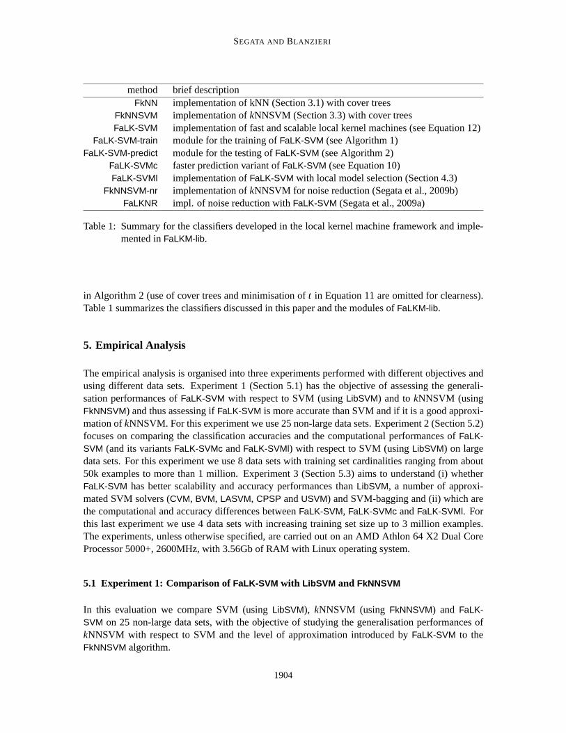
Table 1: Summary for the classifiers developed in the local kernel machine framework and imple-mented inFaLKM-lib.
in Algorithm 2 (use of cover trees and minimisation oft in Equation 11 are omitted for clearness).Table 1 summarizes the classifiers discussed in this paper and the modules ofFaLKM-lib.
5. Empirical Analysis
The empirical analysis is organised into three experiments performed with different objectives andusing different data sets. Experiment 1 (Section 5.1) has the objective ofassessing the generali-sation performances ofFaLK-SVM with respect to SVM (usingLibSVM) and tokNNSVM (usingFkNNSVM) and thus assessing ifFaLK-SVM is more accurate than SVM and if it is a good approxi-mation ofkNNSVM. For this experiment we use 25 non-large data sets. Experiment 2 (Section 5.2)focuses on comparing the classification accuracies and the computational performances ofFaLK-SVM (and its variantsFaLK-SVMc andFaLK-SVMl) with respect to SVM (usingLibSVM) on largedata sets. For this experiment we use 8 data sets with training set cardinalities ranging from about50k examples to more than 1 million. Experiment 3 (Section 5.3) aims to understand (i) whetherFaLK-SVM has better scalability and accuracy performances thanLibSVM, a number of approxi-mated SVM solvers (CVM, BVM, LASVM, CPSP andUSVM) and SVM-bagging and (ii) which arethe computational and accuracy differences betweenFaLK-SVM, FaLK-SVMc andFaLK-SVMl. Forthis last experiment we use 4 data sets with increasing training set size up to 3 million examples.The experiments, unless otherwise specified, are carried out on an AMDAthlon 64 X2 Dual CoreProcessor 5000+, 2600MHz, with 3.56Gb of RAM with Linux operating system.
5.1 Experiment 1: Comparison ofFaLK-SVM with LibSVM and FkNNSVM
In this evaluation we compare SVM (usingLibSVM), kNNSVM (using FkNNSVM) and FaLK-SVM on 25 non-large data sets, with the objective of studying the generalisation performances ofkNNSVM with respect to SVM and the level of approximation introduced byFaLK-SVM to theFkNNSVM algorithm.
1904

FAST AND SCALABLE LOCAL KERNEL MACHINES
data set # of # of class data set # of # of classname features points balancing name features points balancing
sonar 60 208 53%/47% fourclass 2 862 64%/36%heart 13 270 56%/44% tic-tac-toe 9 958 65%/35%
mushrooms 112 300 53%/47% mam 5 961 54%/46%haberman 3 306 74%/26% numer 24 1000 70%/30%
liver 6 345 58%/42% splice 60 1000 52%/48%ionosphere 34 351 64%/36% spambase 57 1000 57%/43%
vote 15 435 61%/39% vehicle 21 1243 76%/24%musk1 166 476 57%/43% cmc 7 1473 57%/43%
hill-valley 100 606 51%/49% ijcnn1 22 1500 68%/32%breast 10 683 65%/35% a1a 123 1605 76%/24%
australian 14 690 56%/44% chess 35 2130 52%/48%transfusion 4 748 76%/24% astro 4 3089 65%/35%
diabetes 8 768 65%/35%
Table 2: The 25 binary-class data sets of Experiment 1.
5.1.1 EXPERIMENTAL PROTOCOL
The data sets are listed in Table 2; they are retrieved from the UCI (Asuncion and Newman, 2007)and STATLOG (Michie et al., 1994) repositories, with cardinality between 200 and 3100 points(some data sets have been randomly sub-sampled), dimensionality lower than 200, not very unbal-anced, and they are all scaled in the[0,1] interval. The comparison is carried out using three differentkernel functions (linear, RBF and homogeneous polynomial), in a 10-foldCV experimental setting.Internal to each training fold the model selection is performed with a nested 10-fold CV choosingthe parameters in the following ranges. The regularisation parameterC is chosen for all methods inthe set{2−2,2−1, . . . ,29,210}, the width parameterσ of the RBF kernel in{2−5,2−4, . . . ,22,23}, thedegree of the polynomial kernels in{1,2,3}. The neighbourhood parameterk for FkNNSVM andFaLK-SVM is selected by the cross-validation procedure in the set{21,22, . . . , 29,210, |X |} where|X | is the cardinality of the training set,5 while thek′ parameter ofFaLK-SVM is fixed tok/2 whichis a value that privileges scalability over accuracy because we want to test a value that can permitgood computational results for large and very large data sets.
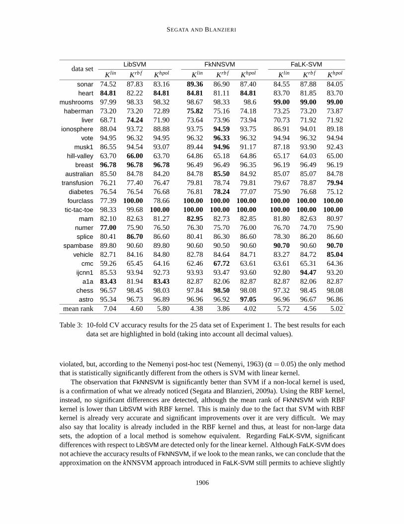
5.1.2 RESULTS AND DISCUSSION
Table 3 reports the accuracy results of all tested methods and kernels. Inaddition to the mean ranksreported in the figure, we assessed the statistical significance of the differences between pairs ofmethods using the Wilcoxon Signed Rank Test (Wilcoxon, 1945; Demsar, 2006) withα = 0.05.The test highlights thatFkNNSVM is significantly better thanLibSVM for the linear and polynomialkernels, whereas for the RBF kernel no significant differences aredetected, although the mean rankof FkNNSVM with RBF kernel is lower thanLibSVM with RBF kernel. Applied toFaLK-SVM, theWilcoxon Signed Rank Test detects a significant difference with respectto LibSVM only for thelinear kernel. If we perform the Friedman test (Friedman, 1940) (α = 0.05), the null hypothesis is
5. For data set with less than 1024 points somek values are of course not tested.
1905
SEGATA AND BLANZIERI
data setLibSVM FkNNSVM FaLK-SVM
K lin Krb f Khpol K lin Krb f Khpol K lin Krb f Khpol
sonar 74.52 87.83 83.16 89.36 86.90 87.40 84.55 87.88 84.05heart 84.81 82.22 84.81 84.81 81.11 84.81 83.70 81.85 83.70
mushrooms 97.99 98.33 98.32 98.67 98.33 98.6 99.00 99.00 99.00haberman 73.20 73.20 72.89 75.82 75.16 74.18 73.25 73.20 73.87
liver 68.71 74.24 71.90 73.64 73.96 73.94 70.73 71.92 71.92ionosphere 88.04 93.72 88.88 93.75 94.59 93.75 86.91 94.01 89.18
vote 94.95 96.32 94.95 96.32 96.33 96.32 94.94 96.32 94.94musk1 86.55 94.54 93.07 89.44 94.96 91.17 87.18 93.90 92.43
hill-valley 63.70 66.00 63.70 64.86 65.18 64.86 65.17 64.03 65.00breast 96.78 96.78 96.78 96.49 96.49 96.35 96.19 96.49 96.19
australian 85.50 84.78 84.20 84.78 85.50 84.92 85.07 85.07 84.78transfusion 76.21 77.40 76.47 79.81 78.74 79.81 79.67 78.8779.94
diabetes 76.54 76.54 76.68 76.81 78.24 77.07 75.90 76.68 75.12fourclass 77.39 100.00 78.66 100.00 100.00 100.00 100.00 100.00 100.00
tic-tac-toe 98.33 99.68 100.00 100.00 100.00 100.00 100.00 100.00 100.00mam 82.10 82.63 81.27 82.95 82.73 82.85 81.80 82.63 80.97
numer 77.00 75.90 76.50 76.30 75.70 76.00 76.70 74.70 75.90splice 80.41 86.70 86.60 80.41 86.30 86.60 78.30 86.20 86.60
spambase 89.80 90.60 89.80 90.60 90.50 90.60 90.70 90.60 90.70vehicle 82.71 84.16 84.80 82.78 84.64 84.71 83.27 84.7285.04
cmc 59.26 65.45 64.16 62.46 67.72 63.61 63.61 65.31 64.36ijcnn1 85.53 93.94 92.73 93.93 93.47 93.60 92.8094.47 93.20
a1a 83.43 81.94 83.43 82.87 82.06 82.87 82.87 82.06 82.87chess 96.57 98.45 98.03 97.84 98.50 98.08 97.32 98.45 98.08astro 95.34 96.73 96.89 96.96 96.92 97.05 96.96 96.67 96.86
mean rank 7.04 4.60 5.80 4.38 3.86 4.02 5.72 4.56 5.02
Table 3: 10-fold CV accuracy results for the 25 data set of Experiment 1. The best results for eachdata set are highlighted in bold (taking into account all decimal values).
violated, but, according to the Nemenyi post-hoc test (Nemenyi, 1963) (α = 0.05) the only methodthat is statistically significantly different from the others is SVM with linear kernel.
The observation thatFkNNSVM is significantly better than SVM if a non-local kernel is used,is a confirmation of what we already noticed (Segata and Blanzieri, 2009a). Using the RBF kernel,instead, no significant differences are detected, although the mean rankof FkNNSVM with RBFkernel is lower thanLibSVM with RBF kernel. This is mainly due to the fact that SVM with RBFkernel is already very accurate and significant improvements over it arevery difficult. We mayalso say that locality is already included in the RBF kernel and thus, at leastfor non-large datasets, the adoption of a local method is somehow equivalent. RegardingFaLK-SVM, significantdifferences with respect toLibSVM are detected only for the linear kernel. AlthoughFaLK-SVM doesnot achieve the accuracy results ofFkNNSVM, if we look to the mean ranks, we can conclude that theapproximation on thekNNSVM approach introduced inFaLK-SVM still permits to achieve slightly
1906

FAST AND SCALABLE LOCAL KERNEL MACHINES
data set # of train. testing class originalname feat. points points balancing source
ijcnn1 22 49990 91701 90%/10% LibSVM rep. (Chang and Lin, 2001)cov-type * 54 100000 481010 51%/49% LibSVM rep. (Chang and Lin, 2001)census-inc 41 199523 99762 94%/6% UCI rep. (Asuncion and Newman, 2007)
cod-rna 8 364651 121549 67%/33% (Uzilov et al., 2006)intr-det 40 1026588 311029 79%/21% UCI KDD rep. (Hettich and Bay, 1999)
2-spirals * 2 100000 100000 50%/50% Synthetic (Segata and Blanzieri, 2009c)ndcc * 5 100000 100000 61%/39% Synthetic (Thompson, 2006)
checker-b * 2 300000 100000 50%/50% Synthetic (e.g., see Tsang et al., 2005)
Table 4: The 8 large data sets of the second empirical experiment. The data sets whose extensionsare used also in Experiment 3 are denoted with *.
better results than SVM also on non-large data sets, confirming our preliminary analysis (Segata andBlanzieri, 2009c). These results also indicates that theE[λ] term introduced in the risk ofFaLK-SVM(Section 4.4), due to the approximations introduced to thekNNSVM approach, is small enough toassure higher generalisation accuracies with respect to SVM.
The overall outcome of this experiment is thatFaLK-SVM is a good approximation ofFkNNSVMthat maintains a little advantage over SVM and it is particularly effective with the RBF kernel withrespect to linear and polynomial kernels. Notice that the experiment is carried out using small datasets in which locality is very likely to play a marginal role differently from large data sets in whichit can be crucial.
5.2 Experiment 2: FaLK-SVM, FaLK-SVMc and FaLK-SVMl vs. LibSVM and FkNN on LargeData Sets
In this experiment we applyFaLK-SVM, FaLK-SVMc, FaLK-SVMl, LibSVM on 8 large data setscomparing the computational and generalisation performances using the RBFkernel, because pre-liminary experiments showed that the linear or polynomial kernels have very low accuracy resultson the considered problems. We also add to the comparison the kNN classifier(implemented withcover trees and calledFkNN) using the Euclidean distance.
5.2.1 EXPERIMENTAL PROTOCOL
The data sets considered in this experiment are listed in Table 4 with the corresponding sources andare all scaled in the[0,1] interval. They range from a training set cardinality of about 50k pointsto more than one million, whereas the dimensionality is not high (always under 60) with separatedtest sets. In order to select the parameters a 10-fold CV procedure is performed in the trainingset (apart fromFaLK-SVMl) choosing the values in the following sets:C ∈ {2−2,2−1, . . . ,29,210},σ ∈ {2−15,2−14, . . . ,24,25}, k for FaLK-SVM in {250,500,1000,2000,4000,8000} with k′ = k/2,andk for FkNNSVM in {1,3,5,9,15,21,31,51,71,101,151}. FaLK-SVM does not necessarily testall values fork because if the maximum empirical accuracy is found for a specific value ofk,for examplek = 500, and for the following value, in this casek = 1000, the maximum is lower,the remaining higher values ofk are not tested. Due to the computational resources necessary
1907

SEGATA AND BLANZIERI
data setFkNN LibSVM FaLK-SVM FaLK-SVMc FaLK-SVMl
10f-CV test 10f-CV test 10f-CV test 10f-CV test test
ijcnn1 97.37 96.64 98.99 97.98 99.04 98.04 98.96 97.98 98.03cov-type 91.73 91.99 92.60 92.83 92.68 92.89 92.44 92.60 92.84
census-inc 94.53 94.52 95.14 95.13 95.07 95.07 95.00 94.99 94.99cod-rna 95.88 96.25 97.18 97.17 97.19 97.23 97.06 97.09 97.29intr-det 99.74 92.04 99.89 91.77 99.74 91.97 99.69 92.01 91.91
2-spirals 88.43 88.43 85.18 85.29 88.42 88.47 88.29 88.45 88.30ndcc 85.47 84.99 86.66 86.21 86.63 86.29 86.33 85.93 86.24
checker-b 94.31 94.08 94.46 94.21 94.46 94.21 94.45 94.19 94.23test acc.
4.25 3.25 1.63 3.38 2.50mean rank
Table 5: Empirical (using 10-fold CV) and generalisation accuracies ofFkNN, LibSVM, FaLK-SVM,FaLK-SVMc andFaLK-SVMl on the 8 large data sets of Experiment 2. The best generalisa-tion accuracy for each data set is highlighted in bold. The last line reports the mean rankof each method among the 8 data sets.
for performing model selection, especially forLibSVM, we performed the cross-validation runson a Linux-based TORQUE cluster with 20 nodes. ForFaLK-SVMl the local model selection isperformed on 10 local models,C∈ {20,22,24,26}, k∈ {500,1000,2000,4000}, σ locally estimatedwith the 1st, 10th, 50th or 90th percentile of the distribution of the distances.
5.2.2 RESULTS AND DISCUSSION
Table 5 reports the generalisation accuracies of the analysed classifiers. Looking at the mean ranks,we can see thatFaLK-SVM is the most accurate (it achieves the best results in half of the data sets),followed by FaLK-SVMl. LibSVM andFaLK-SVMc seem to perform very similar but little worsethanFaLK-SVM andFaLK-SVMl. Not surprisingly,FkNN performs poorly in almost all the data sets,except for theintr-det data set in which it achieves the best result. According to the Wilcoxon SignedRank Test (Wilcoxon, 1945; Demsar, 2006)FaLK-SVM is significantly more accurate thanLibSVM,whereas, excludingFkNN, no other significant differences are detected. Apart for theintr-det dataset that has slightly different distribution in the training and testing sets (some types of networkattacks are present in the test set only), the best empirical accuracies are always very similar to thegeneralisation accuracies meaning that all techniques avoid over-fitting.
Table 6 reports the training times together with the speed-ups ofFaLK-SVM, FaLK-SVMc andFaLK-SVMl with respect toLibSVM. We can notice that the speed-ups achieved byFaLK-SVM andFaLK-SVMc are always greater than 4.7, and in the majority of the cases they are at least one orderof magnitude bigger thanLibSVM. Generally,FaLK-SVMc turns out to be faster thanFaLK-SVMalthough the two classifiers implement the same training algorithm. This happens because the modelselection chooses forFaLK-SVMc a lower value ofk with respect toFaLK-SVM. In fact,FaLK-SVMcis less accurate thanFaLK-SVM in choosing the nearest model for a testing point, and this causes anhigher value of theE[λ] constant that increases the risk ofFaLK-SVMc with respect toFaLK-SVM(see Equation 14 and Equation 15). So using a lowerk (and thus a lowerk′) tends to have more
1908

FAST AND SCALABLE LOCAL KERNEL MACHINES
data setLibSVM FaLK-SVM FaLK-SVMc FaLK-SVMl
training training speed-up training speed-up train. time speed-uptime (s) time (s) onLibSVM time (s) onLibSVM with l.m.s. onLibSVM
ijcnn1 102 15 6.8 15 6.8 1850 0.1cov-type 8362 88 95.0 38 220.1 1214 6.9
census-inc 13541 6047 4.7 2391 5.7 10271 1.3cod-rna 9777 395 24.8 225 43.5 579 16.9intr-det 5262 286 18.4 284 18.5 450 11.7
2-spirals 4043 188 21.5 81 49.9 3442 1.2ndcc 1487 302 4.9 92 16.2 4609 0.3
checker-b 6047 334 18.1 366 16.5 1374 4.4
Table 6: Training times for Experiment 2 ofLibSVM, FaLK-SVM, FaLK-SVMc andFaLK-SVMl andthe speed-ups of the three local methods with respect toLibSVM. The best training timefor each data set is highlighted in bold.
data setLibSVM FaLK-SVM FaLK-SVMc FaLK-SVMl
testing testing speed-up testing speed-up testing speed-uptime (s) time (s) onLibSVM time (s) onLibSVM time (s) onLibSVM
ijcnn1 43 32 1.3 5 8.6 36 1.2cov-type 2795 202 13.8 73 38.3 191 14.6
census-inc 597 1347 0.4 58 10.3 1328 0.4cod-rna 396 261 1.5 58 6.8 259 1.5intr-det 192 146 1.3 76 2.5 149 1.3
2-spirals 957 10 95.7 5 191.4 18 53.2ndcc 148 61 2.4 7 21.1 61 2.4
checker-b 167 10 16.7 7 23.9 7 23.9
Table 7: Testing times for Experiment 2 ofLibSVM, FaLK-SVM, FaLK-SVMc andFaLK-SVMl andthe speed-ups of the three local methods with respect toLibSVM. The best testing time foreach data set is highlighted in bold.
models in the proximity of the testing point making the choice less problematic.FaLK-SVMl issometimes slower thanLibSVM, but we have to consider thatFaLK-SVMl includes model selection,whereas for the other methods the time needed by model selection is not considered in the trainingtime, so, practically speaking,FaLK-SVMl is the fastest method if the optimal parameters are notapriori known.
The testing times required by the analysed methods are reported in Table 7. AsexpectedFaLK-SVMc is the fastest among all methods with speed-up overLibSVM ranging from more than 2 toalmost 200.FaLK-SVM andFaLK-SVMl are also generally faster thanLibSVM with only one case inwhich the testing time is about two times slower.
This experiment shows that for 8 non high-dimensional data sets, our approach outperforms astate-of-the-art accurate SVM solver both in terms of generalisation accuracies and computational
1909

SEGATA AND BLANZIERI
performances. Although we have an additional parameter to tune (k), FaLK-SVM andFaLK-SVMcare faster enough to maintain the performance advantages overLibSVM also for model selection(we choosek in a small set of values). Moreover, withFaLK-SVMl we addressed the problem ofmodel selection with a specific approach to set the parameters;FaLK-SVMl outperformsLibSVM ingeneralisation accuracy, and the time it needs for both internal model selection and training is atleast comparable (faster in 7 cases on a total of 8) with the timeLibSVM needs for the training only.
5.3 Experiment 3: Comparison of Scalability Performances ofFaLK-SVM, FaLK-SVMc,FaLK-SVMl, LibSVM and Approximated SVM Solvers
In this experiment we test the scalability performances of our techniques (FaLK-SVM, FaLK-SVMc,FaLK-SVMl) on training sets with increasing sizes using the RBF kernel against several other tech-niques. The techniques taken into account areLibSVM, the approximated SVM solvers calledCVM,LASVM, USVM, BVM, CPSP (Section 2.3), SVM-bagging with fixed dimension of the sub-sampledtraining sets (SVM-B) and SVM-bagging with fixed proportion of the sub-sampled training sets withrespect to the whole training set (SVM-Bs). Although we apply all the classifiers with the same pro-tocol on the same data sets, we report, for clearness, the results in two parts: the comparison ofFaLK-SVM with LibSVM and the approximated SVM solvers in Section 5.3.2, the comparison ofFaLK-SVM with its variantsFaLK-SVMc andFaLK-SVMl in Section 5.3.3.
5.3.1 EXPERIMENTAL PROTOCOL
We consider here the data sets of Table 4 for which we can further enlarge the training set size.The data sets for which we can add sets of new training examples are thecov-type data set (fulltraining set of 500k points) and the three artificial data sets named2-spirals, ndcc andchecker-b (upto 3 million points). Forcov-type the testing set is reduced to 50k examples (the other examplesare added to the training set) so the accuracy results are not directly comparable to the previousexperiment.
The model selection for all the classifiers (with the exception ofFaLK-SVMl that performs in-ternally a local model selection) is performed on the smallest training set only,using the chosenparameter for all the higher training set sizes. This is necessary, especially for LibSVM and approx-imated SVM solvers, for computational reasons. ForLibSVM, BVM, CVM, USVM (with the convexconcave procedure) andCPSP, we performed cross validation forC andσ using the same setting ofthe previous experiment. The default threshold valueε for the stopping criteria are maintained: 10−3
for LibSVM, FaLK-SVM, LASVM and 10−1 for CPSP while CVM andBVM automatically choose thevalue ofε based on the data at each application. We set the same size of the kernel cache (100M)for all the methods. The maximum number of core vectors forCVM andBVM is 50000 (the defaultvalue), the maximum number of basis vectors forCPSP is set to 1000. ForSVM-B andSVM-Bs weneed to set respectively the size and the proportion of the sub-sampled training sets and the param-eters of the SVMs. ForSVM-B the size of the sub-sampled training sets is equal to the 5% of theoriginal training sets of each data set (namely 100000 forcov-type, 2-spirals andndcc and 300000for checker-b), whereasSVM-Bs maintains the same sampling rate (5%) for all the applicationsand so the cardinality of the sub-sampled training sets increases with the cardinality of the trainingset. BothSVM-B andSVM-Bs train 101 SVMs and the prediction is performed using the majorityvoting. The value of 101 is chosen because it is a sufficient high number for allowing good accura-cies and it is an odd number preventing possible ties in the majority voting. The parameters of the
1910

FAST AND SCALABLE LOCAL KERNEL MACHINES
SVM for SVM-B andSVM-Bs (usingLibSVM) are chosen using model selection with the same gridsof parameters used forLibSVM. We also testedFaLK-SVMl using the same setting of the previousexperiment. Each algorithm is tested for training set sizes requiring no more than 100000 seconds(more than 27 hours) for training.
Since the authors ofBVM (Tsang et al., 2005) andCVM (Tsang et al., 2007) declared the Linuximplementation of their techniques deprecated (see the authors reply to Loosliand Canu (2007)available onBVM webpage), we use the Windows executables on a Intel Pentium D Dual CoreCPU 3.40GHz with 2Gb of RAM running Windows XP instead of the AMD Athlon 64X2 DualCore Processor 5000+, 2600MHz, with 3.56Gb of RAM with Linux operating system used for allthe other classifiers. Because of the use of different operating systemsand hardware forBVM andCVM, their running times should not be directly compared to the others. However,the comparisonis justified by preliminary tests that showed that the Linux version ofBVM on the AMD Athlonmachine and the Windows version ofBVM on the Intel Pentium machine have similar runningtimes.
5.3.2 RESULTS AND DISCUSSION: FALK-SVM VS LIBSVM AND APPROXIMATED SVMSOLVERS
Figure 3 shows the generalisation accuracies of the methods at increasingtraining set sizes. Somemethods do not appear in the figures due to low generalisation results or computational difficultiesthat cause abnormal terminations of the algorithms, and some accuracy results for large trainingset sizes are not present due to the excessive computational time required for training (more than100000 seconds). We can observe that it is very important to use as manypoints as possible inorder to increase the accuracies for thecov-type andndcc data sets. The same consideration canbe done for the2-spirals data, althoughFaLK-SVM already starts from very high accuracies and theincrement is limited, while for thechecker-b data set the increment of the accuracies is negligible foralmost all the methods. For thechecker-b data set, the enlarging of the training set is not motivatedfrom the accuracy viewpoint, but we still use it as a benchmark for the computational performances.
Comparing the generalisation accuracies of Figure 3 among the tested methods, we can seethat FaLK-SVM is almost always on top for each of the four data sets. In this experiment aswellas in the previous ones, we setk′ = k/2; lower values fork′ would probably allowFaLK-SVMto achieve higher accuracy results (although with worse computational performances). However,even if the choice of thek′ parameter can be non-optimal, we decided to avoid the model selectionfor k′ since the results are already satisfactory. The methods that seem to give results comparablewith FaLK-SVM (apart from the2-spirals data set) areLibSVM andUSVM and they are able, in fewcases, to slightly improve theFaLK-SVM results (LibSVM for 2 training set sizes forcov-type andchecker-b, USVM for 2 training set sizes forcov-type andchecker-b and 1 forndcc). The baggingtechniques give high accuracies only for thechecker-b data set; this is not surprising because wealready noticed that for thechecker-b problem the use of large data sets is not required and thussubsampling-based methods likeSVM-B andSVM-Bs are competitive. The results of the online andactive learning approach ofLASVM are slightly lower thanFaLK-SVM, LibSVM andUSVM. CPSPgives acceptable results in only one case, and for the2-spirals andchecker-b data sets it suffers fromnumerical problems possibly due to the scaling of the features in the[0,1] interval. Enlarging themaximum number of basis functions forCPSP gives higher accuracies but the computational timeneeded to build the models is too high. The results we achieve here forLibSVM andLASVM on the
1911

SEGATA AND BLANZIERI
SVM-BsUSVM
LASVMCVM (W)BVM (W)LibSVM
FaLK-SVM
Number of training points×1000
Acc
urac
y(in
perc
enta
ge)
500450400350300250200150100
97
96
95
94
93
92
91
(a) cov-type data set
SVM-BsSVM-BUSVM
LASVMLibSVM
FaLK-SVM
Number of training points×1000
Acc
urac
y(in
perc
enta
ge)
300025002000150010005000
89
88.5
88
87.5
87
86.5
86
85.5
85
(b) 2-spirals data set
SVM-BsSVM-BCPSPUSVM
LASVMLibSVM
FaLK-SVM
Number of training points×1000
Acc
urac
y(in
perc
enta
ge)
300025002000150010005000
87.4
87.2
87
86.8
86.6
86.4
86.2
86
85.8
85.6
(c) ndcc data set
SVM-BsSVM-BUSVM
LASVMLibSVM
FaLK-SVM
Number of training points×1000
Acc
urac
y(in
perc
enta
ge)
300025002000150010005000
94.3
94.25
94.2
94.15
94.1
94.05
94
(d) checker-b data set
Figure 3: Generalisation accuracies ofFaLK-SVM, LibSVM, BVM, CVM, LASVM, USVM, CPSP,SVM-B andSVM-Bs on thecov-type, 2-spirals, ndcc andchecker-b data sets with increas-ing training set sizes (Experiment 3). Some accuracies are missing due to theexcessivecomputational requirements (more than 100000 seconds for training) of thecorrespond-ing method for large training set sizes.
1912

FAST AND SCALABLE LOCAL KERNEL MACHINES
cov-type data sets are a little higher than the results in Bordes et al. (2005) (about 1%better both for100k and 500k training set sizes), and we believe that this is due to the model selection approach weused here that is performed with an exhaustive cross-validation grid search forC andσ. As we cannotice in Figure 3, we observed stability problems forCVM andBVM, even if we used the Windowsbinaries as suggested by the authors.
The training computational performances shown in Figure 4 highlight thatFaLK-SVM is alwaysmuch faster than the alternative techniques that are competitive from the accuracy viewpoint. Infact, althoughCVM, BVM andSVM-B show good scalability performances and in few cases theyovercome the performances ofFaLK-SVM, we noticed from Figure 3 that their generalisation abil-ities are poor. The scaling behaviours ofLibSVM, LASVM andUSVM are very similar (among thethree methodsLibSVM is the fastest forndcc, LASVM is the fastest for2-spirals andUSVM is thefastest forchecker-b) but substantially worse thanFaLK-SVM one (FaLK-SVM is always at least oneorder of magnitude faster with speed-ups increasing with the training set sizes).SVM-Bs is slightlyfaster thanLibSVM but the scalability behaviour is very similar. The methods that achieve acceptableaccuracy results on the smallest training set size (i.e.,LibSVM, LASVM, USVM) are not applicablewhen the number of training examples increases sensibly because of poorcomputational scalabilityperformance; this is evident for the2-spirals, ndcc andchecker-b data sets in which the trainingtimes ofLibSVM, LASVM, USVM exceed 100000 seconds as soon as the training set cardinality ap-proaches one million (the only exception isUSVM that is applicable on 1.5 training examples of thechecker-b data set). On the contrary,FaLK-SVM processes data sets of 3 millions examples in theorder of minutes or few hours. An experiment comparingLibSVM andLASVM on thecov-type dataset with conclusions similar to ours is reported by Bordes et al. (2005) in which howeverLASVM isabout a third faster thanLibSVM whereas hereLibSVM slightly overcomesLASVM; this is probablydue to the fact that forLASVM the only available implementation is the original one by Bordes et al.(2005) whereasLibSVM is frequently updated and improved. Finally,CPSP performs slightly betterthanLibSVM, LASVM andUSVM.
The computational performances of the prediction phase are reported in Figure 5. Also in thiscase the performance ofFaLK-SVM is excellent: onlyCPSP andCVM are faster in 2 data sets thanFaLK-SVM, but their corresponding generalisation accuracies are low. As expected,CPSP achievesvery fast predictions because it limits the number of basis function to 1000 and thus for each testingpoints no more than 1000 kernel functions are computed.LibSVM, LASVM and USVM achievesimilar results also in testing performances and, apart from small training setsfor thendcc data set,they are at least one order of magnitude slower thanFaLK-SVM and the difference grows for largetraining set sizes. The slowest approach isSVM-Bs and this is due to the high number of modelsthat need to be evaluated for each testing point and to the fact that the size of the models increaseswith the training set size. AlsoSVM-B has rather high prediction times but, since the size of themodels is almost constant, also the performances at increasing training sizesare constant. It can beargued that the number of models used for bagging can be lowered to obtainfaster prediction times;however, if we want to achieve the computational performances ofFaLK-SVM we need to use nomore than 20 models (in the worst case) and this seriously affects the prediction accuracies that arealready much lower thanFaLK-SVM ones.
The overall conclusion we can draw about the scalability of the proposedtechniques is that, atleast for these 4 non high-dimensional data sets,FaLK-SVM is substantially better than the state-of-the-art kernel methods for classification, and this is achieved withoutaffecting the accuracyperformances that showed to be always at least as good as the best alternative technique. Apart
1913

SEGATA AND BLANZIERI
SVM-BsSVM-BCPSPUSVM
LASVMCVM (W)BVM (W)LibSVM
FaLK-SVM
Number of training points×1000
Tra
inin
gtim
e(in
sec.
,log
.sc
ale)
500450400350300250200150100
100000
10000
1000
100
10
(a) cov-type data set
SVM-BsSVM-BUSVM
LASVMCVM (W)BVM (W)LibSVM
FaLK-SVM
Number of training points×1000
Tra
inin
gtim
e(in
sec.
,log
.sc
ale)
300025002000150010005000
100000
10000
1000
100
(b) 2-spirals data set
SVM-BsSVM-BCPSPUSVM
LASVMCVM (W)BVM (W)LibSVM
FaLK-SVM
Number of training points×1000
Tra
inin
gtim
e(in
sec.
,log
.sc
ale)
300025002000150010005000
100000
10000
1000
100
(c) ndcc data set
SVM-BsSVM-BLASVM
CVM (W)BVM (W)LibSVM
FaLK-SVM
Number of training points×1000
Tra
inin
gtim
e(in
sec.
,log
.sc
ale)
300025002000150010005000
100000
10000
1000
100
(d) checker-b data set
Figure 4: Training times ofFaLK-SVM, LibSVM, BVM, CVM, LASVM, USVM, CPSP, SVM-B andSVM-Bs on thecov-type, 2-spirals, ndcc andchecker-b data sets with increasing trainingset sizes (Experiment 3). The times (in seconds) are reported in logarithmicscale.
1914
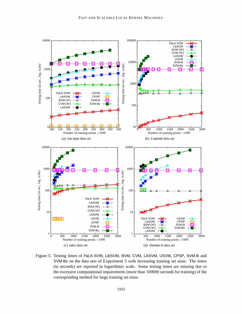
FAST AND SCALABLE LOCAL KERNEL MACHINES
SVM-BsSVM-BCPSPUSVM
LASVMCVM (W)BVM (W)LibSVM
FaLK-SVM
Number of training points×1000
Test
ing
time
(inse
c.,l
og.
scal
e)
500450400350300250200150100
10000
1000
100
10
(a) cov-type data set
SVM-BsSVM-BUSVM
LASVMCVM (W)BVM (W)LibSVM
FaLK-SVM
Number of training points×1000
Test
ing
time
(inse
c.,l
og.
scal
e)
300025002000150010005000
100000
10000
1000
100
10
(b) 2-spirals data set
SVM-BsSVM-BCPSPUSVM
LASVMCVM (W)BVM (W)LibSVM
FaLK-SVM
Number of training points×1000
Test
ing
time
(inse
c.,l
og.
scal
e)
300025002000150010005000
10000
1000
100
10
1
(c) ndcc data set
SVM-BsSVM-BCPSPUSVM
LASVMCVM (W)BVM (W)LibSVM
FaLK-SVM
Number of training points×1000
Test
ing
time
(inse
c.,l
og.
scal
e)
300025002000150010005000
10000
1000
100
10
1
(d) checker-b data set
Figure 5: Testing times ofFaLK-SVM, LibSVM, BVM, CVM, LASVM, USVM, CPSP, SVM-B andSVM-Bs on the data sets of Experiment 3 with increasing training set sizes. The times(in seconds) are reported in logarithmic scale. Some testing times are missing duetothe excessive computational requirements (more than 100000 seconds for training) of thecorresponding method for large training set sizes.
1915

SEGATA AND BLANZIERI
for LibSVM (and consequently forSVM-B andSVM-Bs), we have to say that the available code ofthe other tested techniques has not been recently updated and for this reason it is possible to arguethat higher performances with more optimised implementations of the tested approaches could bereached. It is also necessary to underline that in literatureLASVM, USVM, CPSP, BVM andCVMhave been prevalently tested on data sets with high dimensionality or, apart for cov-type, on datasets not requiring highly non-linear decision functions. The approximatednon-linear SVM solversand bagging approaches we tested could be indicated for data in which the linear kernel is not theoptimal choice, but, at the same time, the decision function can be accurately reconstructed with areduced amount of information (number of examples, support vectors orbasis functions).
5.3.3 RESULTS AND DISCUSSION: COMPARISON BETWEENFALK-SVM, FALK-SVMC AND
FALK-SVML
Figure 6 reports the comparison of the generalisation accuracies ofFaLK-SVM, FaLK-SVMc andFaLK-SVMl at increasing training set size. The computational performances for the training phaseare reported in Figure 7, and for the testing phase in Figure 8.
From the accuracy viewpoint, we can notice that, as expected,FaLK-SVM is almost alwaysslightly more accurate thanFaLK-SVMc. FaLK-SVMl, apart fromchecker-b, is less accurate thanFaLK-SVM for the smaller training set sizes, and this is due to the fact thatFaLK-SVM performs afull grid search for model selection whereasFaLK-SVMl adopts the very fast local model selectionapproach. However,FaLK-SVMl rivals FaLK-SVM as the training set sizes increases. This is rea-sonable becauseFaLK-SVM uses for all the training set sizes the parameters found for the smallertraining sets, and the best cross-validated parameters can differ for sub-sampled sets with differ-ent cardinality. For example, as the number of training points increases, theradius of the localneighbourhoods decreases if we maintain the samek andk′ values, and the original value for thewidth parameter of the RBF kernel can no longer be the optimal one. For this reason, in the case ofcov-type andndcc data sets,FaLK-SVMl achieves higher accuracies thanFaLK-SVM for the largesttraining sets.FaLK-SVMl shows a slightly higher accuracy variability thenFaLK-SVM andFaLK-SVMc at different training set sizes; this is an empirical confirmation that the parameters selectedby FaLK-SVMl can be less stable than the parameters selected with standard cross validation, but thephenomenon seems to be acceptable if not negligible.
The training computational performances of Figure 7 confirm (as alreadydiscussed in Sec-tion 5.2.2) that, althoughFaLK-SVM andFaLK-SVMc make use of the same training algorithm, themodel selection procedure selects lower values ofk for FaLK-SVMc, thus assuring faster trainingtimes thanFaLK-SVM. The speed-ups ofFaLK-SVMc with respect toFaLK-SVM are however neverhigher than one order of magnitude. ForFaLK-SVMl we can notice a somehow irregular behaviourfor increasing dimensions of the training set and this is due to the different values of the neighbour-hood, kernel and regularisation parameters it chooses during the internal fast local model selectionphase. In some casesFaLK-SVMl is significantly slower thanFaLK-SVM. However, the trainingtimes forFaLK-SVMl include the model selection procedure whereas forFaLK-SVM we consideronly the training with the optimal parameters, so we can conclude thatFaLK-SVMl is a good choicefor huge training sets on which traditional model selection becomes intractable.
The testing times reported in Figure 8 confirm thatFaLK-SVMc is always faster thanFaLK-SVMandFaLK-SVMl. In particular, we can notice thatFaLK-SVMc at least halves the testing time ofFaLK-SVM. FaLK-SVMl is computationally very similar toFaLK-SVM. This is not surprising because the
1916

FAST AND SCALABLE LOCAL KERNEL MACHINES
FaLK-SVMlFaLK-SVMcFaLK-SVM
Number of training points×1000
Acc
urac
y(in
perc
enta
ge)
500450400350300250200150100
97
96.5
96
95.5
95
94.5
94
93.5
93
92.5
(a) cov-type data set
FaLK-SVMlFaLK-SVMcFaLK-SVM
Number of training points×1000
Acc
urac
y(in
perc
enta
ge)
300025002000150010005000
88.75
88.7
88.65
88.6
88.55
88.5
88.45
88.4
88.35
88.3
88.25
(b) 2-spirals data set
FaLK-SVMlFaLK-SVMcFaLK-SVM
Number of training points×1000
Acc
urac
y(in
perc
enta
ge)
300025002000150010005000
87.4
87.2
87
86.8
86.6
86.4
86.2
(c) ndcc data set
FaLK-SVMlFaLK-SVMcFaLK-SVM
Number of training points×1000
Acc
urac
y(in
perc
enta
ge)
300025002000150010005000
94.3
94.28
94.26
94.24
94.22
94.2
94.18
94.16
94.14
94.12
94.1
(d) checker-b data set
Figure 6: Generalisation accuracies ofFaLK-SVM, FaLK-SVMc and FaLK-SVMl on thecov-type,2-spirals, ndcc andchecker-b data sets with increasing training set sizes (Experiment 3).
1917

SEGATA AND BLANZIERI
FaLK-SVMlFaLK-SVMcFaLK-SVM
Number of training points×1000
Tra
inin
gtim
e(in
sec.
,log
.sc
ale)
500450400350300250200150100
10000
1000
100
10
(a) cov-type data set
FaLK-SVMlFaLK-SVMcFaLK-SVM
Number of training points×1000
Tra
inin
gtim
e(in
sec.
,log
.sc
ale)
300025002000150010005000
100000
10000
1000
100
10
(b) 2-spirals data set
FaLK-SVMlFaLK-SVMcFaLK-SVM
Number of training points×1000
Tra
inin
gtim
e(in
sec.
,log
.sc
ale)
300025002000150010005000
100000
10000
1000
100
(c) ndcc data set
FaLK-SVMlFaLK-SVMcFaLK-SVM
Number of training points×1000
Tra
inin
gtim
e(in
sec.
,log
.sc
ale)
300025002000150010005000
10000
1000
100
(d) checker-b data set
Figure 7: Training times ofFaLK-SVM, FaLK-SVMc, andFaLK-SVMl on thecov-type, 2-spirals,ndcc andchecker-b data sets with increasing training set sizes (Experiment 3). The times(in seconds) are reported in logarithmic scale.
1918

FAST AND SCALABLE LOCAL KERNEL MACHINES
FaLK-SVMlFaLK-SVMcFaLK-SVM
Number of training points×1000
Test
ing
time
(inse
c.,l
og.
scal
e)
500450400350300250200150100
100
10
1
(a) cov-type data set
FaLK-SVMlFaLK-SVMcFaLK-SVM
Number of training points×1000
Test
ing
time
(inse
c.,l
og.
scal
e)
300025002000150010005000
100
10
1
(b) 2-spirals data set
FaLK-SVMlFaLK-SVMcFaLK-SVM
Number of training points×1000
Test
ing
time
(inse
c.,l
og.
scal
e)
300025002000150010005000
1000
100
10
(c) ndcc data set
FaLK-SVMlFaLK-SVMcFaLK-SVM
Number of training points×1000
Test
ing
time
(inse
c.,l
og.
scal
e)
300025002000150010005000
100
10
1
(d) checker-b data set
Figure 8: Testing times ofFaLK-SVM, FaLK-SVMc, andFaLK-SVMl on thecov-type, 2-spirals, ndccandchecker-b data sets with increasing training set sizes (Experiment 3). The times (inseconds) are reported in logarithmic scale.
1919

SEGATA AND BLANZIERI
only difference betweenFaLK-SVM andFaLK-SVMl regards the model selection but both classifiersneed, during testing, to perform a nearest neighbour search of the query points among all trainingexamples, differently fromFaLK-SVMc that performs the nearest neighbour search only among thecentres of the local models.
The FaLK-SVMl results permit us to discuss the sensitivity of the local kernel machine ap-proaches with respect to the neighbourhood parameterk. The local model selection ofFaLK-SVMlselects different values ofk at each application and thek selected byFaLK-SVMl is very often dif-ferent from the value selected byFaLK-SVM with standard model selection. However, the accuracyresults are not very dependent on this as we notice in Figure 6 in which the accuracy variationsof FaLK-SVMl as the training sets increase are rather smooth and the accuracies are very similar toFaLK-SVM. So the sensitivity of the accuracies with respect tok for local kernel machines seems tobe low at least for large data sets. From the computational viewpoint, instead, we know from thecomplexity analysis that the advantages of local kernel machines are effective as long ask is sub-stantially lower thenN. In our experiments the value ofk selected by model selection is bounded to8000; higher values, although not tested, may decrease the computationalperformances.
We can conclude thatFaLK-SVM, FaLK-SVMc and FaLK-SVMl achieve similar accuracy andcomputational results. When the model selection forFaLK-SVM andFaLK-SVMc become computa-tionally intractable,FaLK-SVMl is an option to efficiently perform model selection and thus obtaina lower overall training time. When very low testing times are required,FaLK-SVMc is preferableto FaLK-SVM at the price of a slightly lower generalisation accuracy.
6. Conclusions
In this work, we have introduced a new local kernel-based classifier, calledFaLK-SVM, that is scal-able for large non high-dimensional data. The approach is developed starting from the theory oflocal learning algorithms and in particular from the Local SVM classifier, called kNNSVM. Variousstrategies are introduced to overcome the computational problems ofkNNSVM and to switch froma completely lazy-learning setting to a eager learning setting with efficient predictions. Learningand complexity bounds forFaLK-SVM are favourable if compared with the SVM ones.FaLK-SVMhas, in fact, a training time complexity which is sub-quadratic in the training set size, and a predic-tion time complexity which is logarithmic. A novel approach for model selection, again based onlocality, is introduced obtaining theFaLK-SVMl classifier which substantially unburdens the modelselection strategies based on cross-validation. Another variant of the algorithm, calledFaLK-SVMc,permits to simplify the prediction phase. We thus showed that locality can be usedto developcomputationally efficient classifiers.
We carried out an extensive empirical evaluation of the introduced approaches showing that,for large classification problems requiring non linear decision functions our FaLK-SVM algorithmis much faster and accurate than traditional and approximated SVM solvers.In fact, (i) FaLK-SVMachieves very good accuracy results because it considers all the points without locally under-fittingthe data and (ii)FaLK-SVM is very fast and scalable because the cardinality of the local problemscan be maintained low. The variant calledFaLK-SVMc further enhances testing speed at the price ofa little accuracy loss, and the other variant, calledFaLK-SVMl, decreases the overall training time.
In general, we have showed that locality can be the key not only for obtaining accurate classi-fiers, but also for effectively speeding-up kernel-based algorithms.
1920
FAST AND SCALABLE LOCAL KERNEL MACHINES
Further developments of the approach include a dimensionality reduction preprocessing step inorder to attack also high-dimensional problems, the application of local classifiers different fromSVM, and a distributed parallel version. Also the determination of the critical value of the intrin-sic dimensionality (rather than the number of features) above which the localapproaches are noteffective is still an open question and the answer should be very data-dependent.
References
David W. Aha.Lazy Learning. Kluwer Academic Publishers Norwell, MA, USA, 1997.
Erin L. Allwein, Robert E. Schapire, and Yoram Singer. Reducing multiclass to binary : A unifyingapproach for margin classifiers.Journal of Machine Learning Research, 1:113–141, 2000.
Arthur Asuncion and David Newman. UCI machine learning repository, 2007. URL http://www.ics.uci.edu/ ˜ mlearn/MLRepository.html .
Christopher G. Atkeson, Andrew W. Moore, and Stefan Schaal. Locallyweighted learning.ArtificialIntelligence Review, 11(1-5):11–73, 1997.
Yoshua Bengio, Olivier Delalleau, and Nicolas Le Roux. The curse of highly variable functions forlocal kernel machines. InAdvances in Neural Information Processing Systems, volume 18, 2005.
Alina Beygelzimer, Sham Kakade, and John Langford. Cover trees fornearest neighbor. InTwenty-third International Conference on Machine Learning (ICML 06), pages 97–104, New York, NY,USA, 2006. ACM.
Jock A Blackard and Denis J. Dean. Comparative accuracies of artificial neural networks anddiscriminant analysis in predicting forest cover types from cartographic variables. Computersand Electronics in Agriculture, 24:131–151, 1999.
Enrico Blanzieri and Anton Bryl. Evaluation of the highest probability SVM nearest neighborclassifier with variable relative error cost. InCEAS 2007, Mountain View, California, 2007.
Enrico Blanzieri and Farid Melgani. An adaptive SVM nearest neighbor classifier for remotelysensed imagery. InIEEE International Conference on Geoscience and Remote Sensing Sympo-sium (IGARSS 06), pages 3931–3934, 2006.
Enrico Blanzieri and Farid Melgani. Nearest neighbor classification of remote sensing images withthe maximal margin principle.IEEE Transactions on Geoscience and Remote Sensing, 46(6):1804–1811, 2008.
Antoine Bordes and Leon Bottou. The Huller: A simple and efficient online SVM. InMachineLearning: ECML 2005, Lecture Notes in Artificial Intelligence, LNAI 3720, pages 505–512.Springer Verlag, 2005.
Antoine Bordes, Seyda Ertekin, Jason Weston, and Leon Bottou. Fast kernel classifiers with onlineand active learning.Journal of Machine Learning Research, 6:1579–1619, 2005.
Antoine Bordes, Leon Bottou, and Patrick Gallinari. SGD-QN: Careful quasi-Newton stochasticgradient descent.Journal of Machine Learning Research, 10:1737–1754, July 2009.
1921

SEGATA AND BLANZIERI
Leon Bottou and Vladimir N. Vapnik. Local learning algorithms.Neural Computation, 4(6):888–900, 1992.
Leon Bottou, Corinna Cortes, John S. Denker, Harris Drucker, Isabelle Guyon, Lawrence D. Jackel,Yann Le Cun, Urs A. Muller, Eduard Sackinger, Patrice Simard, and Vladimir Vapnik. Com-parison of classifier methods: A case study in handwritten digit recognition.In Twelveth IAPRInternational Conference on Pattern Recognition, Conference B: Computer Vision & Image Pro-cessing, volume 2, pages 77–82. IEEE, 1994.
Leo Breiman. Bagging predictors.Machine Learning, 24(2):123–140, August 1996.
David Broomhead and David Lowe. Multivariable functional interpolation and adaptive networks.Complex Systems, 2:321–355, 1988.
Chih-Chung Chang and Chih-Jen Lin.LIBSVM: A Library for Support Vector Machines, 2001.Software available athttp://www.csie.ntu.edu.tw/ ˜ cjlin/libsvm .
Kai-Wei Chang, Cho-Jui Hsieh, and Chih-Jen Lin. Coordinate descent method for large-scale l2-loss linear support vector machines.Journal of Machine Learning Research, 9:1369–1398, 2008.
Qun Chang, Qingcai Chen, and Xiaolong Wang. Scaling Gaussian RBF kernel width to improveSVM classification.International Conference on Neural Networks and Brain, 2005. (ICNN&B05), 1:19–22, 2005.
Long Chen. New analysis of the sphere covering problems and optimal polytope approximation ofconvex bodies.Journal of Approximation Theory, 133(1):134, 2005.
Haibin Cheng, Pang-Ning Tan, and Rong Jin. Localized support vectormachine and its efficientalgorithm.SIAM International Conference on Data Mining, 2007.
Vasek Chvatal. A greedy heuristic for the set-covering problem.Mathematics of Operations Re-search, pages 233–235, 1979.
Kenneth L. Clarkson. Nearest neighbor queries in metric spaces. InTwenty-ninth Annual ACMSymposium on Theory of computing (STOC 97), pages 609–617, New York, NY, USA, 1997.ACM.
Michael Collins, Amir Globerson, Terry Koo, Xavier Carreras, and Peter L. Bartlett. Exponentiatedgradient algorithms for conditional random fields and max-margin markov networks. Journal ofMachine Learning Research, 9:1775–1822, 2008.
Ronan Collobert, Fabian Sinz, Jason Weston, and Leon Bottou. Trading convexity for scalability.In Twenty-third International Conference on Machine Learning (ICML 06), pages 201–208, NewYork, NY, USA, 2006. ACM.
Corinna Cortes and Vladimir Vapnik. Support-vector networks.Machine Learning, 20(3):273–297,1995.
Janez Demsar. Statistical comparisons of classifiers over multiple data sets.Journal of MachineLearning Research, 7:1–30, 2006.
1922
FAST AND SCALABLE LOCAL KERNEL MACHINES
Jian-xiong Dong. Fast SVM training algorithm with decomposition on very large data sets.IEEETransaction Pattern Analysis and Machine Intelligence, 27(4):603–618, 2005. Senior Member-Krzyzak, Adam and Fellow-Suen, Ching Y.
Rong-En Fan, Pai-Hsuen Chen, and Chih-Jen Lin. Working set selection using second order in-formation for training support vector machines.The Journal of Machine Learning Research, 6:1889–1918, 2005.
Rong-En Fan, Kai-Wei Chang, Cho-Jui Hsieh, Xiang-Rui Wang, andChih-Jen Lin. LIBLINEAR: Alibrary for large linear classification.The Journal of Machine Learning Research, 9:1871–1874,2008.
Milton Friedman. A comparison of alternative tests of significance for the problem of m rankings.The Annals of Mathematical Statistics, 11(1):86–92, 1940.
Michael R. Garey and David S. Johnson.Computers and Intractability: A Guide to the Theory ofNP-Completeness. WH Freeman & Co. New York, NY, USA, 1979.
Seth Hettich and Stephen D. Bay. The UCI KDD archive, 1999. URLhttp://kdd.ics.uci.edu .
Cho-Jui Hsieh, Kai-Wei Chang, Chih-Jen Lin, S. Sathiya Keerthi, and S. Sundararajan. A dualcoordinate descent method for large-scale linear SVM. InTwenty-fifth International Conferenceon Machine Learning (ICML 08), pages 408–415, New York, NY, USA, 2008. ACM.
Chih-Wei Hsu and Chih-Jen Lin. A comparison of methods for multiclass support vector machines.IEEE Transactions on Neural Networks, 13(2):415–425, 2002.
Thorsten Joachims. Making large-scale support vector machine learningpractical. Advances inkernel methods: support vector learning, pages 169–184, 1999.
Thorsten Joachims. Training linear SVMs in linear time. InTwelveth ACM SIGKDD InternationalConference on Knowledge Discovery and Data Mining, pages 217–226. ACM New York, NY,USA, 2006.
Thorsten Joachims and Chun-Nam Yu. Sparse kernel SVMs via cutting-plane training. MachineLearning, 2009.
Thorsten Joachims, Thomas Finley, and Chun-Nam John Yu. Cutting-planetraining of structuralSVMs. Machine Learning, 77(1):27–59, 2009.
Michael J. Kearns and Umesh V. Vazirani.An Introduction to Computational Learning Theory.MIT Press Cambridge, MA, USA, 1994.
Sathiya Keerthi and Dennis DeCoste. A modified finite Newton method for fastsolution of largescale linear SVMs.Journal of Machine Learning Research, 6:341–361, 2005.
Sathiya Keerthi, Olivier Chapelle, and Dennis DeCoste. Building support vector machines withreduced classifier complexity.Journal of Machine Learning Research, 7:1493–1515, 2006.
1923

SEGATA AND BLANZIERI
Stefan Knerr, Leon Personnaz, and Gerard Dreyfus. Single-layerlearning revisited: A stepwiseprocedure for building and training a neural network.Optimization Methods and Software, 1:23–34, 1990.
Robert Krauthgamer and James R. Lee. Navigating nets: simple algorithms forproximity search.In Fifteenth Annual ACM-SIAM Symposium on Discrete algorithms (SODA 04), pages 798–807,Philadelphia, PA, USA, 2004. Society for Industrial and Applied Mathematics.
Ulrich H.-G. Kressel. Pairwise classification and support vector machines. Advances in KernelMethods: Support Vector Learning, pages 255–268, 1999.
Yuh-jye Lee and Olvi L. Mangasarian. RSVM: Reduced support vector machines. InFirst SIAMInternational Conference on Data Mining, 2001.
Chih-Jen Lin, Ruby C. Weng, and S. Sathiya Keerthi. Trust region Newton methods for large-scalelogistic regression. InTwenty-fourth International Conference on Machine learning (ICML 07),pages 561–568, New York, NY, USA, 2007. ACM.
Gaelle Loosli and Stephane Canu. Comments on the “Core vector machines: Fast SVM training onvery large data sets”.Journal of Machine Learning Research, 8:291–301, 2007.
Olvi L. Mangasarian. A finite Newton method for classification.Optimization Methods and Soft-ware, 17(5):913–929, 2002.
Mario Marchand and John Shawe-Taylor. The set covering machine.The Journal of MachineLearning Research, 3:723–746, 2003.
Donald Michie, David J. Spiegelhalter, Charles C. Taylor, and John Campbell, editors. MachineLearning, Neural and Statistical Classification. Ellis Horwood, Upper Saddle River, NJ, USA,1994. ISBN 0-13-106360-X.
Paul Nemenyi.Distribution-Free Multiple Comparisons. PhD thesis, Princeton, 1963.
John C. Platt, Nello Cristianini, and John Shawe-Taylor. Large margin DAGsfor multiclass classi-fication. Advances in Neural Information Processing Systems, 12(3):547–553, 2000.
Bernard Scholkopf and Alexander J. Smola.Learning with Kernels: Support Vector Machines,Regularization, Optimization, and Beyond. MIT Press Cambridge, MA, USA, 2002.
Nicola Segata. FaLKM-lib v1.0: A library for fast local kernel machines.Technical Report DISI-09-025, id 1613, DISI, University of Trento, Italy, 2009. Software available athttp://disi.unitn.it/ ˜ segata/FaLKM-lib .
Nicola Segata and Enrico Blanzieri. Empirical assessment of classification accuracy of Local SVM.In Eighteenth Annual Belgian-Dutch Conference on Machine Learning (Benelearn 2009), pages47–55, 2009a.
Nicola Segata and Enrico Blanzieri. Operators for transforming kernels into quasi-local kernels thatimprove SVM accuracy. Technical Report DISI-09-042, id 1652, Tech. rep., DISI, University ofTrento, 2009b.
1924

FAST AND SCALABLE LOCAL KERNEL MACHINES
Nicola Segata and Enrico Blanzieri. Fast local support vector machines for large datasets. InInternational Conference on Machine Learning and Data Mining (MLDM 2009), volume 5632of Lecture Notes in Computer Science. Springer, 2009c.
Nicola Segata, Enrico Blanzieri, and Padraig Cunningham. A scalable noise reduction techniquefor large case-based systems. In L Ginty and D.C Wilson, editors,Case-Based Reasoning Re-search and Development: 8th International Conference on Case-Based Reasoning (ICCBR09),volume 09 ofLecture Notes in Artificial Intelligence, pages 755–758. Springer, 2009a.
Nicola Segata, Enrico Blanzieri, Sarah Jane Delany, and Padraig Cunningham. Noise reduction forinstance-based learning with a local maximal margin approach.Journal of Intelligent InformationSystems, 2009b. In Press.
Shai Shalev-Shwartz, Yoram Singer, and Nathan Srebro. Pegasos:Primal estimated sub-gradientsolver for SVM. InTwenty-fourth International Conference on Machine learning (ICML 07),pages 807–814, New York, NY, USA, 2007. ACM.
Alexander J. Smola, SVN Vishwanathan, and Quoc V. Le. Bundle methods for machine learning.Advances in Neural Information Processing Systems, 20:1377–1384, 2008.
Michael E. Thompson. NDCC: Normally distributed clustered datasets on cubes, 2006.www.cs.wisc.edu/dmi/svm/ndcc/.
Ivor W. Tsang, James T. Kwok, and Pak-Ming Cheung. Core vector machines: Fast SVM trainingon very large data sets.The Journal of Machine Learning Research, 6:363–392, 2005.
Ivor W. Tsang, Andras Kocsor, and James T. Kwok. Simpler core vector machines with enclosingballs. InTwenty-fourth International Conference on Machine Learning (ICML 07), pages 911–918, New York, NY, USA, 2007. ACM.
Andrew V. Uzilov, Joshua M. Keegan, and David H. Mathews. Detection of non-coding rnas on thebasis of predicted secondary structure formation free energy change. BMC Bioinformatics, 7(1):173, 2006.
Vladimir N. Vapnik. The Nature of Statistical Learning Theory. Springer, 2000.
Vladimir N. Vapnik and Leon Bottou. Local algorithms for pattern recognition and dependenciesestimation.Neural Computation, 5(6):893–909, 1993.
Jigang Wang, Predrag Neskovic, and N. Leon Cooper. A minimum spherecovering approach topattern classification.International Conference on Pattern Recognition, 3:433–436, 2006.
Xun-Kai Wei and Ying-Hong Li. Linear programming minimum sphere set covering for extremelearning machines.Neurocomputing, 71(4–6):570–575, 2008.
Frank Wilcoxon. Individual comparisons by ranking methods.Biometrics Bulletin, 1(6):80–83,1945.
Tao Yang and Vojislav Kecman. Adaptive local hyperplane classification.Neurocomputing, 71(13-15):3001–3004, 2008.
1925

SEGATA AND BLANZIERI
Tao Yang and Vojislav Kecman. Adaptive local hyperplane algorithm for learning small medicaldata sets.Expert Systems, 26(4):355–359, 2009.
Tao Yang and Vojislav Kecman. Face recognition with adaptive local hyperplane algorithm.PatternAnalysis & Applications, 13(1):79–83, 2010. ISSN 1433-7541.
Alan L. Yuille and Anand Rangarajan. The concave-convex procedure. Neural Computation, 15(4):915–936, 2003.
Alon Zakai and Ya’acov Ritov. Consistency and localizability.Journal of Machine Learning Re-search, 10:827–856, 2009.
Luca Zanni, Thomas Serafini, and Gaetano Zanghirati. Parallel softwarefor training large scalesupport vector machines on multiprocessor systems.Journal of Machine Learning Research, 7:1467–1492, 2006.
Hao Zhang, Alexander C. Berg, Michael Maire, and Jitendra Malik. SVM-KNN: Discriminativenearest neighbor classification for visual category recognition.IEEE Computer Society Confer-ence on Computer Vision and Pattern Recognition, 2:2126–2136, 2006.
1926


![Scalable Mobile Visual Classification by Kernel Preserving ...ycsu/publications/tmm2013su.pdf · geNet dataset [1], which contains more than 20,000 concepts, has enabled such studies](https://img.pdfslide.net/doc/110x75/5f1d996521a6761df267678f/scalable-mobile-visual-classiication-by-kernel-preserving-ycsupublicationstmm2013supdf.jpg)