Ceterum in problematis natura fundatum est, ut methodi quaecunque continuo prolixioresevadant, quo maiores sunt numeri, ad quos applicantur.[It is in the nature of the problem that any method will become more prolix as the numbersto which it is applied grow larger.]

— Carl Friedrich Gauß, Disquisitiones Arithmeticae (1801)English translation by A.A. Clarke (1965)

Illam vero methodum calculi mechanici taedium magis minuere, praxis tentantem docebit.[Truly, that method greatly reduces the tedium of mechanical calculations; practice willteach whoever tries it.]

— Carl Friedrich Gauß, “Theoria interpolationis methodo nova tractata” (c. 1805)

After much deliberation, the distinguished members of the international committee decidedunanimously (when the Russian members went out for a caviar break) that since theChinese emperor invented the method before anybody else had even been born, the methodshould be named after him. The Chinese emperor’s name was Fast, so the method wascalled the Fast Fourier Transform.

— Thomas S. Huang, “How the fast Fourier transform got its name” (1971)

AFast Fourier Transforms

[Read Chapters 0 and 1 first.]Status: Beta

A.1 Polynomials

Polynomials are functions of one variable built from additions, subtractions, and multipli-cations (but no divisions). The most common representation for a polynomial p(x) is asa sum of weighted powers of the variable x:

p(x) =n∑

j=0

a j xj .

The numbers a j are called the coefficients of the polynomial. The degree of the polynomialis the largest power of x whose coefficient is not equal to zero; in the example above, thedegree is at most n. Any polynomial of degree n can be represented by an array P[0 .. n]of n+ 1 coefficients, where P[ j] is the coefficient of the x j term, and where P[n] 6= 0.

Here are three of the most common operations performed on polynomials:

© 2018 Jeff Erickson http://algorithms.wtf 1

A. FAST FOURIER TRANSFORMS

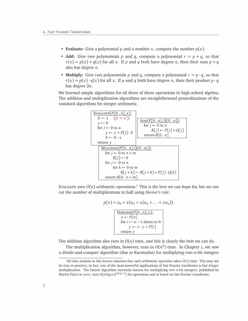
• Evaluate: Give a polynomial p and a number x , compute the number p(x).

• Add: Give two polynomials p and q, compute a polynomial r = p + q, so thatr(x) = p(x) + q(x) for all x . If p and q both have degree n, then their sum p + qalso has degree n.

• Multiply: Give two polynomials p and q, compute a polynomial r = p · q, so thatr(x) = p(x) · q(x) for all x . If p and q both have degree n, then their product p · qhas degree 2n.

We learned simple algorithms for all three of these operations in high-school algebra.The addition and multiplication algorithms are straightforward generalizations of thestandard algorithms for integer arithmetic.

Evaluate(P[0 .. n], x):X ← 1 ⟨⟨X = x j⟩⟩y ← 0for j← 0 to n

y ← y + P[ j] · XX ← X · x

return y

Add(P[0 .. n],Q[0 .. n]):for j← 0 to n

R[ j]← P[ j] +Q[ j]return R[0 .. n]

Multiply(P[0 .. n],Q[0 .. m]):for j← 0 to n+m

R[ j]← 0for j← 0 to n

for k← 0 to mR[ j + k]← R[ j + k] + P[ j] ·Q[k]

return R[0 .. n+m]

Evaluate uses O(n) arithmetic operations.1 This is the best we can hope for, but we cancut the number of multiplications in half using Horner’s rule:

p(x) = a0 + x(a1 + x(a2 + . . .+ xan)).

Horner(P[0 .. n], x):y ← P[n]for i← n− 1 down to 0

y ← x · y + P[i]return y

The addition algorithm also runs in O(n) time, and this is clearly the best we can do.The multiplication algorithm, however, runs in O(n2) time. In Chapter 1, we saw

a divide-and-conquer algorithm (due to Karatsuba) for multiplying two n-bit integers

1All time analysis in this lecture assumes that each arithmetic operation takes O(1) time. This may notbe true in practice; in fact, one of the most powerful applications of fast Fourier transforms is fast integermultiplication. The fastest algorithm currently known for multiplying two n-bit integers, published byMartin Fürer in 2007, uses O(n log n 2O(log∗ n)) bit operations and is based on fast Fourier transforms.

2

A.2. Alternate Representations

in only O(nlg3) steps; precisely the same approach can be applied here. Even clevererdivide-and-conquer strategies lead to multiplication algorithms whose running times arearbitrarily close to linear—O(n1+ε) for your favorite value e > 0—but except for a fewsimple cases, these algorithms not worth the trouble in practice, thanks to large hiddenconstants.

A.2 Alternate Representations

Part of what makes multiplication so much harder than the other two operations isour input representation. Coefficient vectors are the most common representation forpolynomials, but there are at least two other useful representations.

Roots

The Fundamental Theorem of Algebra states that every polynomial p of degree n hasexactly n roots r1, r2, . . . rn such that p(r j) = 0 for all j. Some of these roots maybe irrational; some of these roots may by complex; and some of these roots may berepeated. Despite these complications, this theorem implies a unique representation ofany polynomial of the form

p(x) = sn∏

j=1

(x − r j)

where the r j ’s are the roots and s is a scale factor. Once again, to represent a polynomialof degree n, we need a list of n+ 1 numbers: one scale factor and n roots.

Given a polynomial in this root representation, we can clearly evaluate it in O(n)time. Given two polynomials in root representation, we can easily multiply them in O(n)time by multiplying their scale factors and just concatenating the two root sequences.

Unfortunately, if we want to add two polynomials in root representation, we’re outof luck. There’s essentially no correlation between the roots of p, the roots of q, andthe roots of p + q. We could convert the polynomials to the more familiar coefficientrepresentation first—this takes O(n2) time using the high-school algorithms—but there’sno easy way to convert the answer back. In fact, for most polynomials of degree 5 ormore in coefficient form, it’s impossible to compute roots exactly.2

Samples

Our third representation for polynomials comes from a different consequence of theFundamental Theorem of Algebra. Given a list of n + 1 pairs {(x0, y0), (x1, y1), . . . ,(xn, yn)}, there is exactly one polynomial p of degree n such that p(x j) = y j for all j. Thisis just a generalization of the fact that any two points determine a unique line, because a

2This is where numerical analysis comes from.

3

A. FAST FOURIER TRANSFORMS

line is the graph of a polynomial of degree 1. We say that the polynomial p interpolatesthe points (x j , y j). As long as we agree on the sample locations x j in advance, we onceagain need exactly n+ 1 numbers to represent a polynomial of degree n.

Adding or multiplying two polynomials in this sample representation is easy, as longas they use the same sample locations x j . To add the polynomials, just add their samplevalues. To multiply two polynomials, just multiply their sample values; however, if we’remultiplying two polynomials of degree n, we must start with 2n+ 1 sample values foreach polynomial, because that’s how many we need to uniquely represent their product.Both algorithms run in O(n) time.

Unfortunately, evaluating a polynomial in this representation is no longer straightfor-ward. The following formula, due to Lagrange, allows us to compute the value of anypolynomial of degree n at any point, given a set of n+ 1 samples.

p(x) =n−1∑

j=0

y j∏

k 6= j(x j − xk)

∏

k 6= j

(x − xk)

!

Hopefully it’s clear that formula actually describes a polynomial function of x , sinceeach term in the sum is a scaled product of monomials. It’s also not hard to verify thatp(x j) = y j for every index j; most of the terms of the sum vanish. As I mentionedearlier, the Fundamental Theorem of Algebra implies that p is the only polynomial thatinterpolates the points {(x j , y j)}. Lagrange’s formula can be translated mechanicallyinto an O(n2)-time algorithm.

Summary

We find ourselves in the following frustrating situation. We have three representationsfor polynomials and three basic operations. Each representation allows us to almosttrivially perform a different pair of operations in linear time, but the third takes at leastquadratic time, if it can be done at all!

representation evaluate add multiplycoefficients O(n) O(n) O(n2)roots + scale O(n) ∞ O(n)

samples O(n2) O(n) O(n)

A.3 Converting Between Representations

What we need are fast algorithms to convert quickly from one representation to another.Then if we need to perform an operation that’s hard for our default representation, wecan switch to a different representation that makes the operation easy, perform thedesired operation, and then switch back. This strategy immediately rules out the root

4

A.3. Converting Between Representations

representation, since (as I mentioned earlier) finding roots of polynomials is impossiblein general, at least if we’re interested in exact results.

So how do we convert from coefficients to samples and back? Clearly, once wechoose our sample positions x j , we can compute each sample value y j = p(x j) in O(n)time from the coefficients using Horner’s rule. So we can convert a polynomial of degreen from coefficients to samples in O(n2) time. Lagrange’s formula can be used to convertthe sample representation back to the more familiar coefficient form. If we use the naïvealgorithms for adding and multiplying polynomials (in coefficient form), this conversiontakes O(n3) time.

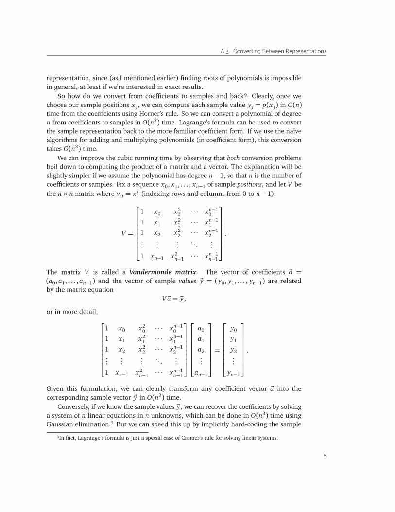
We can improve the cubic running time by observing that both conversion problemsboil down to computing the product of a matrix and a vector. The explanation will beslightly simpler if we assume the polynomial has degree n−1, so that n is the number ofcoefficients or samples. Fix a sequence x0, x1, . . . , xn−1 of sample positions, and let V bethe n× n matrix where vi j = x j

i (indexing rows and columns from 0 to n− 1):

V =

1 x0 x20 · · · xn−1

0

1 x1 x21 · · · xn−1

1

1 x2 x22 · · · xn−1

2...

......

. . ....

1 xn−1 x2n−1 · · · xn−1

n−1

.

The matrix V is called a Vandermonde matrix. The vector of coefficients ~a =(a0, a1, . . . , an−1) and the vector of sample values ~y = (y0, y1, . . . , yn−1) are relatedby the matrix equation

V ~a = ~y ,

or in more detail,

1 x0 x20 · · · xn−1

0

1 x1 x21 · · · xn−1

1

1 x2 x22 · · · xn−1

2...

......

. . ....

1 xn−1 x2n−1 · · · xn−1

n−1

a0

a1

a2...

an−1

=

y0

y1

y2...

yn−1

.

Given this formulation, we can clearly transform any coefficient vector ~a into thecorresponding sample vector ~y in O(n2) time.

Conversely, if we know the sample values ~y , we can recover the coefficients by solvinga system of n linear equations in n unknowns, which can be done in O(n3) time usingGaussian elimination.3 But we can speed this up by implicitly hard-coding the sample

3In fact, Lagrange’s formula is just a special case of Cramer’s rule for solving linear systems.

5

A. FAST FOURIER TRANSFORMS

positions into the algorithm, To convert from samples to coefficients, we can simplymultiply the sample vector by the inverse of V , again in O(n2) time:

~a = V−1 ~y .

Computing V−1 would take O(n3) time if we had to do it from scratch using Gaussianelimination, but because we fixed the set of sample positions in advance, the matrix V−1

can be hard-coded directly into the algorithm.4

So we can convert from coefficients to samples and back in O(n2) time. At first lance,this result seems pointless; we can already add, multiply, or evaluate directly in eitherrepresentation in O(n2) time, so why bother? But there’s a degree of freedom we haven’texploited yet: We get to choose the sample positions! Our conversion algorithm is slowonly because we’re trying to be too general. If we choose a set of sample positions withthe right recursive structure, we can perform this conversion more quickly.

A.4 Divide and Conquer

Any polynomial of degree at most n − 1 can be expressed as a combination of twopolynomials of degree at most (n/2)− 1 as follows:

p(x) = peven(x2) + x · podd(x2).

The coefficients of peven are just the even-degree coefficients of p, and the coefficients ofpodd are just the odd-degree coefficients of p. Thus, we can evaluate p(x) by recursivelyevaluating peven(x2) and podd(x2) and performing O(1) additional arithmetic operations.

Now call a set X of n values collapsing if either of the following conditions holds:• X has one element.

• The set X 2 =�

x2�

� x ∈ X

has exactly n/2 elements and is (recursively) collapsing.Clearly the size of any collapsing set is a power of 2. Given a polynomial p of degreen− 1, and a collapsing set X of size n, we can compute the set {p(x) | x ∈ X } of samplevalues as follows:

1. Recursively compute�

peven(x2)�

� x ∈ X

=�

peven(y)�

� y ∈ X 2

.

2. Recursively compute�

podd(x2)�

� x ∈ X

=�

podd(y)�

� y ∈ X 2

.

3. For each x ∈ X , compute p(x) = peven(x2) + x · podd(x2).The running time of this algorithm satisfies the familiar recurrence T (n) = 2T (n/2) +Θ(n), which as we all know solves to T (n) = Θ(n log n).

4Actually, it is possible to invert an n×n matrix in o(n3) time, using fast matrix multiplication algorithmsthat closely resemble Karatsuba’s sub-quadratic divide-and-conquer algorithm for integer/polynomialmultiplication. On the other hand, my numerical-analysis colleagues have reasonable cause to shoot me inthe face for daring to suggest, even in passing, that anyone actually invert a matrix at all, ever.

6

A.5. The Discrete Fourier Transform

Great! Now all we need is a sequence of arbitrarily large collapsing sets. The simplestmethod to construct such sets is just to invert the recursive definition: If X is a collapsibleset of size n that does not contain the number 0, then

pX = {±

px | x ∈ X } is a collapsible

set of size 2n. This observation gives us an infinite sequence of collapsible sets, startingas follows:5

X1 := {1}X2 := {1, −1}X4 := {1, −1, i, −i}

X8 :=

�

1, −1, i, −i,

p2

2+p

22

i, −p

22−p

22

i,

p2

2−p

22

i, −p

22+p

22

i

�

A.5 The Discrete Fourier Transform

For any n, the elements of Xn are called the complex nth roots of unity; these are theroots of the polynomial xn − 1= 0. These n complex values are spaced exactly evenlyaround the unit circle in the complex plane. Every nth root of unity is a power of theprimitive nth root

ωn = e2πi/n = cos2πn+ i sin

2πn

.

A typical nth root of unity has the form

ωkn = e(2πi/n)k = cos

�

2πn

k�

+ i sin�

2πn

k�

.

These complex numbers have several useful properties for any integers n and k:• There are exactly n different nth roots of unity: ωk

n =ωk mod nn .

• If n is even, then ωk+n/2n = −ωk

n; in particular, ωn/2n = −ω0

n = −1.

• 1/ωkn =ω

−kn =ωk

n = (ωn)k, where the bar represents complex conjugation: a+ bi =a− bi

• ωn =ωkkn. Thus, every nth root of unity is also a (kn)th root of unity.

These properties imply immediately that if n is a power of 2, then the set of all nth rootsof unity is collapsible!

If we sample a polynomial of degree n− 1 at the nth roots of unity, the resulting listof sample values is called the discrete Fourier transform of the polynomial (or more

5In this chapter, lower case italic i always represents the square root of −1. Computer scientists areused to thinking of i as an integer index into a sequence, an array, or a for-loop, but we obviously can’tdo that here. The engineers’ habit of using j =

p−1 just delays the problem—How do engineers write

quaternions?—and typographical hacks like I or i or ι or Mathematica’s ıı◦ are just stupid.

7

A. FAST FOURIER TRANSFORMS

formally, of its coefficient vector). Thus, given an array P[0 .. n− 1] of coefficients, itsdiscrete Fourier transform is the vector P∗[0 .. n− 1] defined as follows:

P∗[ j] := p(ω jn) =

n−1∑

k=0

P[k] ·ω jkn

As we already observed, the fact that sets of roots of unity are collapsible implies that wecan compute the discrete Fourier transform in O(n log n) time. The resulting algorithm,called the fast Fourier transform, was popularized by Cooley and Tukey in 1965.6 Thealgorithm assumes that n is a power of two; if necessary, we can just pad the coefficientvector with zeros.

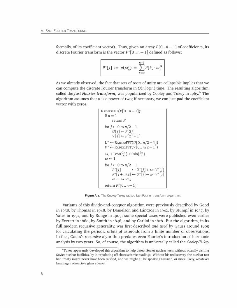
Radix2FFT(P[0 .. n− 1]):if n= 1

return P

for j← 0 to n/2− 1U[ j]← P[2 j]V [ j]← P[2 j + 1]

U∗← Radix2FFT(U[0 .. n/2− 1])V ∗← Radix2FFT(V [0 .. n/2− 1])

ωn← cos( 2πn ) + i sin( 2π

n )ω← 1

for j← 0 to n/2− 1P∗[ j] ← U∗[ j] +ω · V ∗[ j]P∗[ j + n/2]← U∗[ j]−ω · V ∗[ j]ω←ω ·ωn

return P∗[0 .. n− 1]

Figure A.1. The Cooley-Tukey radix-2 fast Fourier transform algorithm.

Variants of this divide-and-conquer algorithm were previously described by Goodin 1958, by Thomas in 1948, by Danielson and Lánczos in 1942, by Stumpf in 1937, byYates in 1932, and by Runge in 1903; some special cases were published even earlierby Everett in 1860, by Smith in 1846, and by Carlini in 1828. But the algorithm, in itsfull modern recursive generality, was first described and used by Gauss around 1805for calculating the periodic orbits of asteroids from a finite number of observations.In fact, Gauss’s recursive algorithm predates even Fourier’s introduction of harmonicanalysis by two years. So, of course, the algorithm is universally called the Cooley-Tukey

6Tukey apparently developed this algorithm to help detect Soviet nuclear tests without actually visitingSoviet nuclear facilities, by interpolating off-shore seismic readings. Without his rediscovery, the nuclear testban treaty might never have been ratified, and we might all be speaking Russian, or more likely, whateverlanguage radioactive glass speaks.

8

A.6. More General Factoring

algorithm. Gauss’s work built on earlier research on trigonometric interpolation byBernoulli, Lagrange, Clairaut, and Euler; in particular, the first explicit description of thediscrete “Fourier” transform was published by Clairaut in 1754, more than half a centurybefore Fourier’s work. Alas, nobody will understand you if you talk about Gauss’s fastClairaut transform algorithms. Hooray for Stigler’s Law!7

A.6 More General Factoring

The algorithm in Figure A.1 is often called the radix-2 fast Fourier transform todistinguish it from other FFT algorithms. In fact, both Gauss and (much later) Cooleyand Tukey described a more general divide-and-conquer strategy that does not assume nis a power of two, but can be applied to any composite order n. Specifically, if n= pq,we can decompose the discrete Fourier transform of order n into simpler discrete Fouriertransforms as as follows. For all indices 0≤ a < p and 0≤ b < q, we have

x∗aq+b =pq−1∑

`=0

x jp+k (ωjp+kpq )`

=p−1∑

k=0

q−1∑

j=0

x jp+kω(aq+b)( jp+k)pq

=p−1∑

k=0

q−1∑

j=0

x jp+kωb jq ω

bkpqω

akp

=p−1∑

k=0

q−1∑

j=0

x jp+k (ωbq)

j

!

ωbkpq

!

(ωap)

k,

The innermost sum in this expression is one coefficient of a discrete Fourier transformof order q, and the outermost sum is one coefficient of a discrete Fourier transform oforder q. The intermediate factors ωbk

pq are now formally known as “twiddle factors”.

7Lest anyone believe that Stigler’s Law has treated Gauss unfairly, remember that “Gaussian elimination”was not discovered by Gauss; the algorithm was not even given that name until the mid-20th century!Elimination became the standard method for solving systems of linear equations in Europe in the early1700s, when it appeared in Isaac Newton’s influential textbook Arithmetica universalis.8 Although Newtonapparently (and perhaps even correctly) believed he had invented the elimination algorithm, it actuallyappears in several earlier works, including the eighth chapter of the Chinese manuscript The Nine Chaptersof the Mathematical Art. The authors and precise age of the Nine Chapters are unknown, but commentarywritten by Liu Hui in 263ce claims that the text was already several centuries old. It was almost certainlynot invented by a Chinese emperor named Fast.

8Arithmetica universalis was compiled from Newton’s lecture notes and published over Newton’sstrenuous objections. He refused to have his name associated with the book, and he even considered buyingup every copy of the first printing to destroy them. Apparently he didn’t want anyone to think it was hislatest research. The first edition crediting Newton as the author did not appear until 25 years after his death.

9

A. FAST FOURIER TRANSFORMS

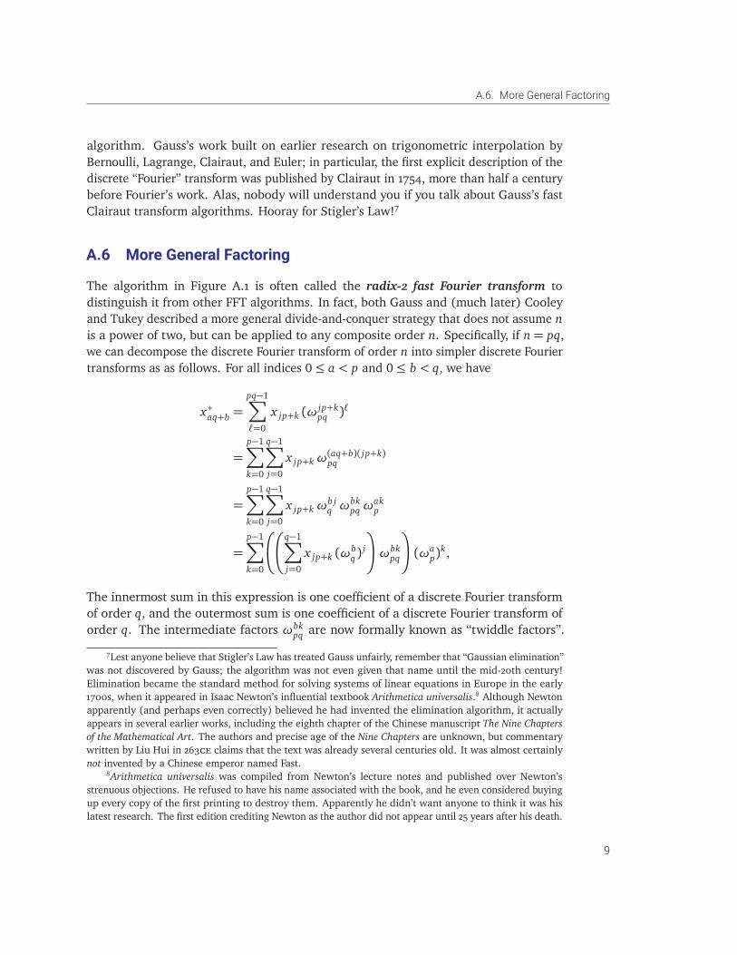
No, seriously, that’s actually what they’re called. This wall of symbols implies that thediscrete Fourier transform of order n can be evaluated as follows:

1. Write the input vector into a p× q array in row-major order.2. Apply a discrete Fourier transform of order p to each column of the 2d array.3. Multiply each entry of the 2d array by the appropriate twiddle factor.4. Apply a discrete Fourier transform of order q to each row of the 2d array.5. Extract the output vector from the p× q array in column-major order.

The algorithm is described in more detail in Figure A.2.

FactorFFT(P[0 .. pq− 1]):⟨⟨Copy/typecast to 2d array in row-major order⟩⟩for j← 0 to p− 1

for k← 0 to q− 1A[ j, k]← P[ jp+ k]

⟨⟨Recursively apply order-p FFTs to columns⟩⟩for k← 0 to q− 1

B[·, k]← FFT(A[·, k])

⟨⟨Multiply by twiddle factors⟩⟩for j← 0 to p− 1

for k← 0 to q− 1B[·, k]← B[·, k] ·ω jk

pq

⟨⟨Recursively apply order-q FFTs to rows⟩⟩for j← 0 to p− 1

C[ j, ·]← FFT(C[ j, ·])

⟨⟨Copy/typecast to 1d array in column-major order⟩⟩for j← 0 to p− 1

for k← 0 to q− 1P∗[ j + kq]← C[ j, k]

return P∗[0 .. pq− 1]

Figure A.2. The Gauss-Cooley-Tukey FFT algorithm

We can recover the original radix-2 FFT algorithm in Figure A.1 by setting p = n/2and q = 2. The lines P∗[ j]← U∗[ j]+ω ·V ∗[ j] and P∗[ j+ n/2]← U∗[ j]−ω ·V ∗[ j] areapplying an order-2 discrete Fourier transform; in particular, the multipliers ω and −ωare the “twiddle factors”.

Both Gauss9 and Cooley and Tukey recommended applying this factorization ap-proach recursively. Cooley and Tukey observed further that if all prime factors of n are

9Gauss wrote: “Nulla iam amplius explicatione opus erit, quomodo illa partitio adhuc ulterius extendiet ad eum casum applicari possit, ubi multitudo omnium valorum propositorum numerus e tribus pluribusvefactoribus compositus est, e.g. si numerus µ rursus esset compositus, in quo casu manifesto quaevis periodus µterminorum in plures periodos minores subdividi potest.” [“There is no need to explain how that division canbe extended further and applied to the case where most of the proposed values are composed of three ormore factors, for example, if the number µ is again composite, in which case each period of µ terms can

10

A.7. Inverting the FFT

smaller than some constant, so that the subproblems at the leaves of the recursion treecan be solved in O(1) time, the entire algorithm runs in only O(n log n) time.

Using a completely different approach, Charles Rader and Leo Bluestein describedFFT algorithms that run in O(n log n) time when n is an arbitrary prime number, byreducing to two FFTs whose orders have only small prime factors. Combining these twoapproaches yields an O(n log n)-time algorithm to compute discrete Fourier transformsof any order n.

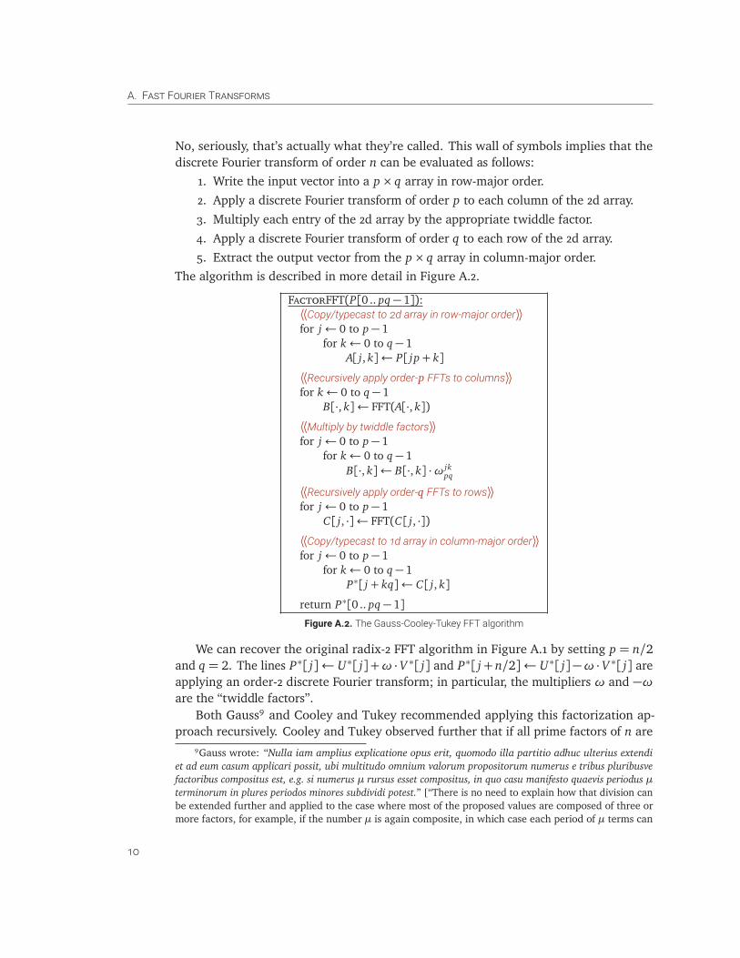
A.7 Inverting the FFT

We also need to recover the coefficients of the product from the new sample values.Recall that the transformation from coefficients to sample values is linear; the samplevector is the product of a Vandermonde matrix V and the coefficient vector. For thediscrete Fourier transform, each entry in V is an nth root of unity; specifically,

v jk =ωjkn

for all integers j and k. More explicitly:

V =

1 1 1 1 · · · 1

1 ωn ω2n ω3

n · · · ωn−1n

1 ω2n ω4

n ω6n · · · ω2(n−1)

n

1 ω3n ω6

n ω9n · · · ω3(n−1)

n...

......

.... . .

...1 ωn−1

n ω2(n−1)n ω3(n−1)

n · · · ω(n−1)2n

To invert the discrete Fourier transform, converting sample values back to coefficients,it suffices to multiply the vector P∗ of sample values by the inverse matrix V−1. Thefollowing amazing fact implies that this is almost the same as multiplying by V itself:

Lemma A.1. V−1 = V/n

Proof: We just have to show that M = V V is the identity matrix scaled by a factor of n.We can compute a single entry in M as follows:

m jk =n−1∑

l=0

ω jln ·ωn

lk =n−1∑

l=0

ω jl−lkn =

n−1∑

l=0

(ω j−kn )l

obviously be subdivided into several smaller periods.”]

11

A. FAST FOURIER TRANSFORMS

If j = k, then ω j−kn =ω0

n = 1, so

m jk =n−1∑

l=0

1= n,

and if j 6= k, we have a geometric series

m jk =n−1∑

l=0

(ω j−kn )l =

(ω j−kn )n − 1

ωj−kn − 1

=(ωn

n)j−k − 1

ωj−kn − 1

=1 j−k − 1

ωj−kn − 1

= 0. �

In other words, if W = V−1 then w jk = v jk/n = ωjkn /n = ω

− jkn /n. What this

observation implies for us computer scientists is that any algorithm for computing thediscrete Fourier transform can be trivially adapted or modified to compute the inversetransform as well; see Figure A.3.

InverseFFT(P∗[0 .. n− 1]):P[0 .. n− 1]← FFT(P∗)for j← 0 to n− 1

P∗[ j]← P∗[ j]/nreturn P[0 .. n− 1]

InverseRadix2FFT(P∗[0 .. n− 1]):if n= 1

return P

for j← 0 to n/2− 1U∗[ j]← P∗[2 j]V ∗[ j]← P∗[2 j + 1]

U ← InverseRadix2FFT(U∗[0 .. n/2− 1])V ← InverseRadix2FFT(V ∗[0 .. n/2− 1])

ωn← cos( 2πn )− i sin( 2π

n )ω← 1

for j← 0 to n/2− 1P[ j] ← (U[ j] +ω · V [ j])/2P[ j + n/2]← (U[ j]−ω · V [ j])/2ω←ω ·ωn

return P[0 .. n− 1]

Figure A.3. Generic and radix-2 inverse FFT algorithms.

A.8 Fast Polynomial Multiplication

Finally, given two polynomials p and q, represented by an arrays of length m and n,respectively, we can multiply them in Θ((m+ n) log(m+ n)) arithmetic operations asfollows. First, pad the coefficient vectors with zeros to length m+n (or to the next largerpower of 2 if we plan to use the radix-2 FFT algorithm). Then compute the discreteFourier transforms of each coefficient vector, and multiply the resulting sample valuesone by one. Finally, compute the inverse discrete Fourier transform of the resultingsample vector.

12

A.9. Inside the Radix-2 FFT

FFTMultiply(P[0 .. m− 1],Q[0 .. n− 1]):for j← m to m+ n− 1

P[ j]← 0for j← n to m+ n− 1

Q[ j]← 0

P∗← FFT(P)Q∗← FFT(Q)for j← 0 to 2` − 1

R∗[ j]← P∗[ j] ·Q∗[ j]return InverseFFT(R∗)

Figure A.4. Multiplying polynomials in O((m+ n) log(m+ n)) time.

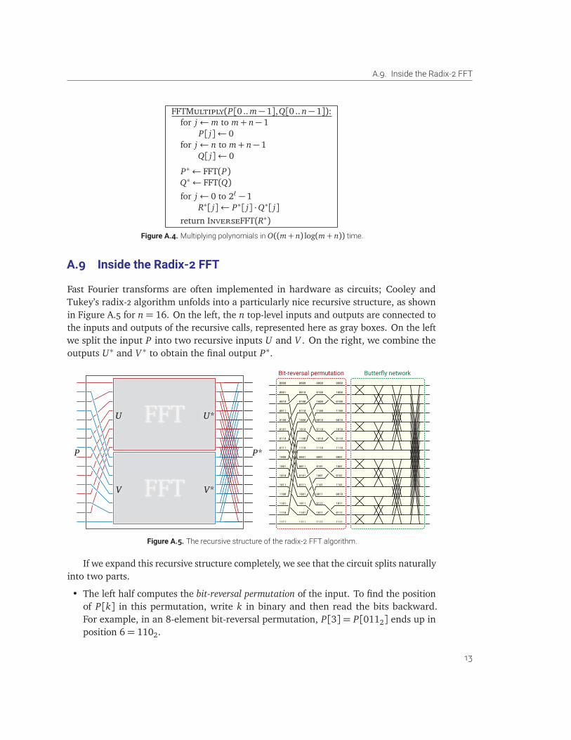
A.9 Inside the Radix-2 FFT

Fast Fourier transforms are often implemented in hardware as circuits; Cooley andTukey’s radix-2 algorithm unfolds into a particularly nice recursive structure, as shownin Figure A.5 for n= 16. On the left, the n top-level inputs and outputs are connected tothe inputs and outputs of the recursive calls, represented here as gray boxes. On the leftwe split the input P into two recursive inputs U and V . On the right, we combine theoutputs U∗ and V ∗ to obtain the final output P∗.

P

FFT

FFT

U U*

V V*

P*

0000

0001

0010

0011

0100

0101

0110

0111

1000

1001

1010

1011

1100

1101

1110

1111

0000

0010

0100

0110

1000

1010

1100

1110

0001

0011

0101

0111

1001

1011

1101

1111

0000

0100

1000

1100

0010

0110

1010

1110

0001

0101

1001

1101

0011

0111

1011

1111

0000

1000

0100

1100

0010

1010

0110

1110

0001

1001

0101

1101

0010

1011

0111

1111

Butterfly networkBit-reversal permutation

Figure A.5. The recursive structure of the radix-2 FFT algorithm.

If we expand this recursive structure completely, we see that the circuit splits naturallyinto two parts.

• The left half computes the bit-reversal permutation of the input. To find the positionof P[k] in this permutation, write k in binary and then read the bits backward.For example, in an 8-element bit-reversal permutation, P[3] = P[0112] ends up inposition 6= 1102.

13

A. FAST FOURIER TRANSFORMS

• The right half of the FFT circuit is called a butterfly network. Butterfly networks areoften used to route between processors in massively-parallel computers, becausethey allow any two processors to communicate in only O(log n) steps.

When n is a power of 2, recursively applying the more general FactorFFT gives usexactly the same recursive structure, just clustered differently. For many applications ofFFTs, including polynomial multiplication, the bit-reversal permutation is unnecessaryand can actually be omitted.

Exercises

1. For any two sets X and Y of integers, the Minkowski sum X + Y is the set of allpairwise sums {x + y | x ∈ X , y ∈ Y }.

(a) Describe an analyze and algorithm to compute the number of elements in X + Yin O(n2 log n) time. [Hint: The answer is not always n2.]

(b) Describe and analyze an algorithm to compute the number of elements in X + Yin O(M log M) time, where M is the largest absolute value of any element ofX ∪ Y . [Hint: What’s this lecture about?]

2. Supposewe are given a bit string B[1 .. n]. A triple of distinct indices 1≤ i < j < k ≤ nis called a well-spaced triple in B if B[i] = B[ j] = B[k] = 1 and k− j = j − i.

(a) Describe a brute-force algorithm to determine whether B has a well-spaced triplein O(n2) time.

(b) Describe an algorithm to determine whether B has a well-spaced triple inO(n log n) time. [Hint: Hint.]

(c) Describe an algorithm to determine the number of well-spaced triples in B inO(n log n) time.

3. (a) Describe an algorithm that determines whether a given set of n integers containstwo elements whose sum is zero, in O(n log n) time.

(b) Describe an algorithm that determines whether a given set of n integers containsthree elements whose sum is zero, in O(n2) time.

(c) Now suppose the input set X contains only integers between − 10000n and10000n. Describe an algorithm that determines whether X contains threeelements whose sum is zero, in O(n log n) time. [Hint: Hint.]

4. Describe an algorithm that applies the bit-reversal permutation to an array A[1 .. n]in O(n) time when n is a power of 2.

14

Exercises

BIT- ⇐⇒ BTI-

REVERSAL ⇐⇒ RRVAESEL

BUTTERFLYNETWORK ⇐⇒ BYEWTEFRUNROTTLK

THISISTHEBITREVERSALPERMUTATION! ⇐⇒ TREUIPRIIAIATRVNHSBTSEEOSLTTHME!

5. The FFT algorithm we described in this lecture is limited to polynomials with 2k

coefficients for some integer k. Of course, we can always pad the coefficient vectorwith zeros to force it into this form, but this padding artificially inflates the inputsize, leading to a slower algorithm than necessary.

Describe and analyze a similar DFT algorithm that works for polynomials with3k coefficients, by splitting the coefficient vector into three smaller vectors of length3k−1, recursively computing the DFT of each smaller vector, and correctly combiningthe results.

6. Fix an integer k. For any two k-bit integers i and j, let i ∧ j denote their bitwiseAnd, and let Σ(i) denote the number of 1s in the binary expansion of i. For example,when k = 4, we have 10∧ 7= 1010∧ 0111= 0010= 2 and Σ(7) = Σ(0111) = 3.

The kth Sylvester-Hadamard matrix Hk is a 2k × 2k matrix indexed by k-bitintegers, each of whose entries is either +1 or −1, defined as follows:

Hk[i, j] = (−1)Σ(i∧ j)

For example:

H3 =

+1 +1 +1 +1 +1 +1 +1 +1

+1 −1 +1 −1 +1 −1 +1 −1

+1 +1 −1 −1 +1 +1 −1 −1

+1 −1 −1 +1 +1 −1 −1 +1

+1 +1 +1 +1 −1 −1 −1 −1

+1 −1 +1 −1 −1 +1 −1 +1

+1 +1 −1 −1 −1 −1 +1 +1

+1 −1 −1 +1 −1 +1 +1 −1

(a) Prove that the matrix Hk can be decomposed into four copies of Hk−1 as follows:

Hk =

�

Hk−1 Hk−1

Hk−1 −Hk−1

�

(b) Prove that Hk ·Hk = 2k · Ik, where I is the 2k × 2k identity matrix.

15

A. FAST FOURIER TRANSFORMS

(c) For any vector ~x ∈ R2k, the product Hk ~x is called the Walsh-Hadamard trans-

form of ~x . Describe an algorithm to compute the Walsh-Hadamard transform inO(n log n) time, given the integer k and a vector of n= 2k integers as input.

ª7. The discrete Hartley transform of a vector ~x = (x0, x1, . . . , xn−1) is another vector~X = (X0, X1, . . . , Xn−1) defined as follows:

X j =n−1∑

i=0

x i

�

cos�

2πn

i j�

+ sin�

2πn

i j��

Describe an algorithm to compute the discrete Hartley transform in O(n log n) timewhen n is a power of 2.

8. Suppose n is a power of 2. Prove that if we recursively apply the FactorFFT algorithm,factoring of n into arbitrary smaller powers of two, the resulting algorithm still runsin O(n log n) time.

9. Let f : Z→ Z be any function such that 2≤ f (n)≤p

n for all n≥ 4. Prove that therecurrence

T (n) =

1 if n≤ 4

f (n) · T�

nf (n)

�

+n

f (n)· T ( f (n)) + O(n) otherwise

has the solution T (n) = O(n log n). For example, setting f (n) = 2 for all n gives usthe standard mergesort/FFT recurrence.

10. Although the radix-2 FFT algorithm and themore general recursive factoring algorithmboth run in O(n log n) time, the latter algorithm is more efficient in practice (when nis large) due to caching effects.

Consider an idealized two-level memory model, which has an arbitrarily largebut slow main memory and a significantly faster cache that holds the C most recentlyaccessed memory items. The running time of an algorithm in this model is dominatedby the number of cache misses, when the algorithm needs to access a value in memorythat it not stored in the cache.

The number of cache misses seen by the radix-2 FFT algorithm obeys the followingrecurrence:

M(n)≤

¨

2 M(n/2) +O(n) if n> C

O(n) if n≤ C

If the input array is too large to fit in the cache, then every memory access in both theinitial and final for-loops will cause a cache miss, and the recursive calls will causetheir own cache misses. But if the input array is small enough to fit in cache, the

16

Exercises

initial for-loop loads the input into the cache, but there are no more cache misses,even inside the recursive calls.

(a) Solve the previous recurrence for M(n), as a function of both n and C . To simplifythe analysis, assume both n and C are powers of 2.

(b) Suppose we always recursively call FactorFFT with p = C and q = n/C . Howmany cache misses does the resulting algorithm see, as a function of n and C? Tosimplify the analysis, assume n= Ck for some integer k. (In particular, assumeC is a power of 2.)

(c) Unfortunately, it is not always possible for a program (or a compiler) to determinethe size of the cache. Suppose we always recursively call FactorFFT withp = q =

pn. How many cache misses does the resulting algorithm see, as a

function of n and C? To simplify the analysis, assume n= C2kfor some integer k.

© 2018 Jeff Erickson http://algorithms.wtf 17