Fast Hashing Algorithms to Summarize Large Collections · PDF fileTexas A&M CS Technical Report 2008-6-1 June 27, 2008 Fast Hashing Algorithms to Summarize Large Collections of Evolutionary

Texas A&M CS Technical Report 2008-6-1

June 27, 2008

Fast Hashing Algorithms to Summarize Large

Collections of Evolutionary Trees

by

Seung-Jin Sul and Tiffani L. Williams

Department of Computer Science

Texas A&M University

College Station, Texas 77843-3112, USA

E-mail: {sulsj,tlw}@cs.tamu.edu

ABSTRACT

Different phylogenetic methods often yield different inferred trees for the same set of

organisms. Moreover, a single phylogenetic approach (such as a Bayesian analysis) can

produce many trees. Consensus trees and topological distance matrices are often used to

summarize the evolutionary relationships among the trees of interest. These summarization

techniques are implemented in current phylogenetic software packages, but they are inefficient

when applied to large collections of trees. Thus, fast algorithms are needed to compare the

relationships among such large tree collections. We present two fast hash-based algorithms—

HashCS and HashRF—for summarizing large collections of evolutionary trees. HashCS

constructs strict and majority consensus trees, and HashRF computes the Robinson-Foulds

(RF) distance between every pair of trees in the collection. We studied the performance

of our hash-based algorithms on tree collections obtained from Bayesian analyses on three

molecular datasets consisting of 16 taxa (euarchontoglires), 150 taxa (desert algae and green

plants), and 567 taxa (angiosperms). The size of our tree collections range from 128 to 16,384

trees. Our experimental results show that our HashCS algorithm is up to 80% faster than

PAUP*, its closest competitor, and 100 times faster than MrBayes. Our HashRF algorithm

is up to 200% faster than PGM-Hashed, the second fastest RF matrix algorithm. HashRF is

over 100 times faster than PAUP*. Thus, our fast hash-based algorithms provide scientists

with a very powerful tool for analyzing the relationships between the large phylogenetic tree

collections in new and exciting ways.

1 Introduction

We develop two fast algorithms—HashCS and HashRF—to summarize the relationships

that exist among a collection of phylogenetic trees. Our HashCS algorithm is designed to

construct strict and majority consensus trees, which summarize the common evolutionary

relationships among the set of trees into a single output tree. HashRF, on the other hand,

computes a matrix of Robinson-Foulds (RF) distances [9] between every pair of trees. Fig-

ure 1 presents an overview of the summarization techniques of interest (all figures and tables

appear at the end of the manuscript beginning on page 30). Effectively summarizing evolu-

tionary relationships among a collection of trees is important for a number of reasons. First,

phylogenetic analyses often produce hundreds to thousands of trees as the best evolutionary

hypothesis for the organisms of interest. Second, different phylogenetic methods often yield

different inferred trees for the same set of organisms. Comparing the competing evolutionary

hypotheses from a phylogenetic search represents a tremendous data-mining opportunity for

understanding the relationships depicted by the collection of trees.

1.1 Our contributions

The novelty of our HashCS and HashRF algorithms is our use of hash tables, which provides

a convenient and fast approach to store and access the relationships depicted in the tree

collections. Hash tables have been widely used to develop extremely fast bioinformatics

algorithms such as BLAST [1] and FASTA [19] for comparing molecular sequences. Recent

work by us has shown the potential of a hash-based algorithm for computing the RF matrix

quickly [27]. We build upon that work by (i) significantly improving the performance of our

HashRF algorithm, (ii) showing that our hash-based framework can construct consensus trees

quickly, and (iii) comparing the performance of our algorithms across a suite of approaches

and tree collections.

Our experimental study uses tree collections obtained from Bayesian analyses using Mr-

Bayes [12]. The number of taxa, n, of our datasets ranged from 16 to 567 taxa. More

specifically, our collection of Bayesian trees were obtained from analyses on 16 taxa (euar-

chontoglires), 150 taxa (desert algae and green plants), and 567 taxa (angiosperms). The size

of our tree collections, t varied from 128 to 16,384 trees. Our results demonstrate that our

hash-based algorithms provide a general-purpose framework for developing fast consensus

tree and RF distance matrix algorithms. Our HashCS algorithm can build consensus trees

up to 80% faster than PAUP [28] and is several orders of magnitude faster than MrBayes.

For computing the RF matrix, HashRF is up to 200% faster than PGM-Hashed [18], the

second-best competitor, and several orders of magnitude faster than PAUP* and Phylip [8].

Summarization techniques as implemented in widely-used phylogenetic software such as

MrBayes, PAUP*, and Phylip are not competitive with our hashing algorithms. Moreover,

given that the grand challenge in phylogenetics is to infer The Tree of Life, significant reduc-

tions in the running time of summarization algorithms is necessary to handle the increasing

size of evolutionary trees and collections that contain them. For example Hillis et al. visually

compared two Bayesian analyses consisting of 44-taxon trees using a matrix of RF distances

between the trees as input [11]. With HashCS and HashRF algorithms, it becomes possible

to summarize (and later visualize) much larger collections of trees in a reasonable amount of

time. Thus, our hash-based algorithms provide scientists with fast tools for understanding

the evolutionary relationships among their collection of trees in new and intriguing ways.

1.2 Comparison with Previous Work

1.2.1 Consensus tree approaches

A number of different techniques have been developed to summarize tree collections by

building consensus trees. Two recent surveys of consensus methods [3, 6] present a theoretical

2

classification and comparison of various consensus approaches. Day’s algorithm [7] is an

O(nt) time complexity algorithm for computing the strict consensus between t trees, where

each tree consists of n taxa. By representing trees by their post-order sequence with weights

(PSW) [25], Day’s algorithm constructs a special cluster representation which gives the

algorithm the ability to determine in constant time whether a bipartition found in one tree

exists in the other tree. The consensus trees are also computed by MrBayes, Phylip, and

PAUP*, but the underlying algorithms are not described in the literature. Even though the

software for MrBayes are Phylip are freely available, it is unclear as to the exact nature of the

running time of these implementations. For majority trees, Amenta et al. hypothesized that

Phylip’s running time is O((n/w)(tn + x lg x + n2)), where x is the number of bipartitions

found, and w is the number of bits in a machine word [2].

Amenta, Clark, and St. John [2] develop an O(nt) algorithm for computing the majority

consensus tree. Their approach takes advantage of using a hash table and consists of two

major steps: (i) reading the t trees and inserting the relevant bipartition information into

the hash table and (ii) using the bipartition information in the hash table to construct the

majority tree. However, constructing the majority tree from the entries in the hash table

requires an additional traversal of the entire tree collection.

Our HashCS and HashRF algorithms are motivated by Amenta et al.’s work. However,

our work differs from their work in a number of distinct ways. First, Amenta et al. do not

provide an algorithm for computing the RF distance matrix from their work. Secondly, our

HashCS algorithm requires a single traversal of the tree collection to compute both the strict

and majority consensus. Both Amenta and our approach use implicit bipartitions, which is a

much faster representation for our algorithms than n- or k-bit bitstrings. However, by relying

on implicit representations alone, it is impossible to construct the resulting consensus tree.

As a result Amenta et al. must process the entire tree collection a second time. To achieve a

single traversal of the input trees, we use an n-bit bitstring representation of the bipartitions

3

on some of the input trees. This approach appears to work well in practice. Given that

there is no software available for Amenta et al.’s approach, we cannot directly compare the

practical implications of their consensus tree algorithm with our HashCS approach.

The Texas Analysis of Symbolic Phylogenetic Information (TASPI) system is a recently

proposed technique to compute consensus trees [4, 5, 13]. One of the novelties of TASPI is it

incorporates a new format for compactly storing and retrieving phylogenetic trees. Experi-

mental results on several collections of maximum parsimony trees show that the TASPI sys-

tem outperforms PAUP* [28] and TNT [10] in constructing consensus trees. Their maximum

parsimony tree collections—inferred with parsimony ratchet [17, 23] and Rec-I-DCM3 [22]

algorithms—have trees consisting of 328 to 8,506 taxa. The number of trees in the collection

range from 47 to 10,000, where the collections incorporated trees with a diverse range of

parsimony scores. The 10,000 trees were based on the 500-taxon rbcL dataset [20]. The

8,506 taxa dataset consisted of 47 trees. All other collections had 2,505 or fewer trees. An

implementation of the TASPI system does not appear to be available to use for experimen-

tal comparison in this paper. However, since it was demonstrated clearly that TASPI and

PAUP* are much faster than TNT’s consensus algorithm, we do not explore the performance

of TNT in this paper. A comparison of Phylip and MrBayes consensus methods was not

included. Hence, we include those techniques in our study.

1.2.2 RF distance matrix

Both PAUP* and Phylip have routines for computing the symmetric distance between every

pair of trees. Day’s basic algorithm for computing the RF distance between two trees is

easily extended to computing the RF distance matrix for t trees. The resulting complexity

of this algorithm is O(nt2), which runs faster than Day’s RF matrix algorithm in practice.

Pattengale, Gottlieb, and Moret [18] describe a number of exact and approximate RF matrix

algorithms. In this paper, we focus strictly on exact approaches. Hence, we study Pattengale

4

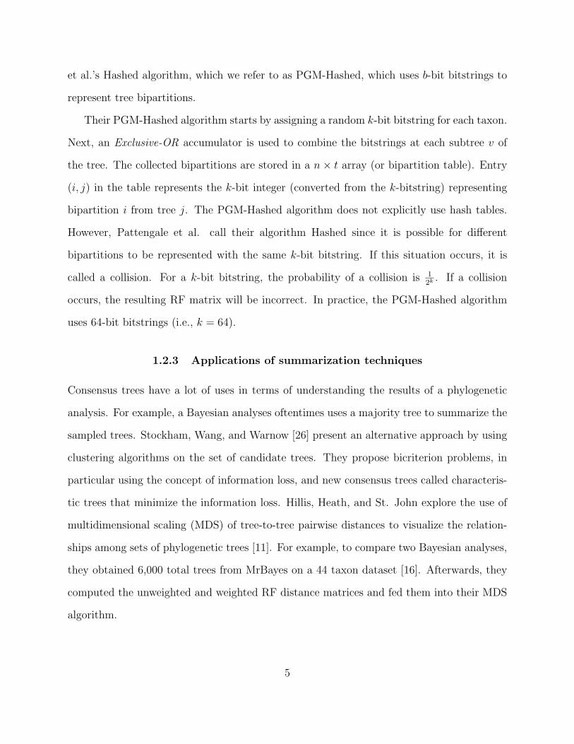
et al.’s Hashed algorithm, which we refer to as PGM-Hashed, which uses b-bit bitstrings to

represent tree bipartitions.

Their PGM-Hashed algorithm starts by assigning a random k-bit bitstring for each taxon.

Next, an Exclusive-OR accumulator is used to combine the bitstrings at each subtree v of

the tree. The collected bipartitions are stored in a n × t array (or bipartition table). Entry

(i, j) in the table represents the k-bit integer (converted from the k-bitstring) representing

bipartition i from tree j. The PGM-Hashed algorithm does not explicitly use hash tables.

However, Pattengale et al. call their algorithm Hashed since it is possible for different

bipartitions to be represented with the same k-bit bitstring. If this situation occurs, it is

called a collision. For a k-bit bitstring, the probability of a collision is 12k . If a collision

occurs, the resulting RF matrix will be incorrect. In practice, the PGM-Hashed algorithm

uses 64-bit bitstrings (i.e., k = 64).

1.2.3 Applications of summarization techniques

Consensus trees have a lot of uses in terms of understanding the results of a phylogenetic

analysis. For example, a Bayesian analyses oftentimes uses a majority tree to summarize the

sampled trees. Stockham, Wang, and Warnow [26] present an alternative approach by using

clustering algorithms on the set of candidate trees. They propose bicriterion problems, in

particular using the concept of information loss, and new consensus trees called characteris-

tic trees that minimize the information loss. Hillis, Heath, and St. John explore the use of

multidimensional scaling (MDS) of tree-to-tree pairwise distances to visualize the relation-

ships among sets of phylogenetic trees [11]. For example, to compare two Bayesian analyses,

they obtained 6,000 total trees from MrBayes on a 44 taxon dataset [16]. Afterwards, they

computed the unweighted and weighted RF distance matrices and fed them into their MDS

algorithm.

5

2 Basics

2.1 Tree bipartitions

In a phylogenetic tree, modern organisms (or taxa) are placed at the leaves and ancestral or-

ganisms occupy internal nodes, with the edges of the tree denoting evolutionary relationships.

Oftentimes, it is useful to represent phylogenies in terms of their bipartitions. Removing an

edge e from a tree separates the leaves on one side from the leaves on the other. The division

of the leaves into two subsets is the bipartition Be associated with edge e. In Figure 2,

tree T1 has two bipartitions: AB|CDE and ABC|DE. An evolutionary tree is uniquely and

completely defined by its set of O(n) bipartitions, where n is the number of taxa. A binary

tree has exactly n − 3 bipartitions.

2.2 Bipartition representations

For each tree in the collection of input trees, we find all of its bipartitions (internal edges)

by performing a depth-first search. In order to process the bipartitions, we need some way

to store them in the computer’s internal memory. Each bipartition in an input tree can be

represented by:

• an n-bitstring, where n is the number of taxa;

• a k-bitstring, where k < n; or

• an implicit representation, which is an integer value, that is constructed by applying a

hashing function to an n-bitstring.

Most of the algorithms studied here use an n-bitstring representation. The PGM-Hashed

approached uses a k-bitstring, and our HashCS and HashRF algorithms use an implicit

representation. Below, we describe the n- and k- bitstring representations. A description of

implicit bipartitions is delayed until we discuss our HashCS algorithm in detail.

6

2.2.1 n-bitstring representation

An intuitive bitstring representation requires n bits, one for each taxon. The first bit is

labeled by the first taxon name, the second bit is represented by the second taxon, etc. We

can represent all of the taxa on one side of the tree with the bit ‘0’ and the remaining taxa

on the side of the tree with the bit ‘1’. Consider the bipartition AB|CDE from tree T1 (see

Figure 2). This bipartition would be represented as 11000, which means that taxa A and

B are one side of the tree, and the remaining taxa are on the other side. Here, taxa on the

same side of a bipartition as taxon A receive a ‘1’.

For each tree in the collection of unrooted input trees, we arbitrarily root the tree. We find

all of its bipartitions (internal edges) by performing a depth-first search traversal performing

an OR operation to the bitstrings of an internal node’s (parent’s) children. Computing the

OR between the two child bipartitions requires visiting each of the n columns of these two

n-bitstrings. If at least one of the bits in column j is a ’1’, then a ’1’ bit is produced for the

column j in the bitstring representation of the parent. Figure 2 presents an example.

2.2.2 k-bitstring representation

The size of the bitstring affects the algorithmic speed. As a result, the PGM-Hashed RF

matrix algorithm [18] use a compressed k-bitstring. Each input taxon is represented by a

random k-bitstring. Similarly to the n-bitstring case, all bipartitions are found by perform-

ing a depth-first search traversal of the tree. However, the bitstrings of an internal node’s

(parent’s) children are exclusive-OR’ed together in the k-bitstring representation. Comput-

ing the exclusive-OR between two child bipartitions requires visiting each of the k columns

of the two k-bitstrings. If the bits in column j are different (same), then a ’1’ (’0’) bit is

produced in column j of the parent node.

There are several consequences of using a compressed bitstring to represent the bipar-

titions of an evolutionary tree. First, it is impossible to tell by looking at the k-bitstring

7

representation of a bipartition what taxa are on different sides of the tree. Hence, it is

impossible to construct consensus trees from k-bitstrings without additional information.

Secondly, there is a possibility that two different bipartitions may in fact be represented

by the same compressed bitstring. If this happens, then the resulting RF matrix will be

incorrect. Pattengale et al. show that the probability of colliding compressed bitstrings

decreases exponentially with the number of bits chosen for representing the bitstrings [18].

However, there are real-world examples when a k-bitstring representation will in fact pro-

duce colliding (i.e., the same) bitstring for different bipartitions. In the implementation of

the PGM-Hashed algorithm, k = 64. Our experimental results show that PGM-Hashed fails

to operate on 567-taxon dataset consisting of 16,384 trees as a result of the high probability

of colliding bipartitions represented by a k-bitstring.

2.3 Consensus trees

Consensus trees summarize the information of a collection of trees into a single output tree.

Bryant provides an excellent survey of different consensus techniques [6]. In this paper, we

consider the most popular consensus approaches: strict consensus and majority trees. The

strict consensus tree contains bipartitions that appear in all of the input trees. To appear

in the majority tree, a bipartition must appear in more than half of the input trees. In

Figure 1, no evolutionary relationship (bipartition) in the tree collection appears in all four

trees. Hence, the resulting strict consensus tree is completely unresolved, which is represented

as a star. The majority consensus tree consists of only the bipartition AB|CDE.

2.4 RF distance

The Robinson-Foulds (RF) distance between two trees is the number of bipartitions that

differ between them. Let Σ(T ) be the set of bipartitions defined by all edges in tree T . The

8

RF distance between two trees Ti and Tj is defined as:

d(Ti, Tj) =|Σ (Ti) − Σ (Tj) | + |Σ (Tj) − Σ (Ti) |

2(1)

PAUP* and Phylip compute the symmetric difference instead of the RF distance. The

symmetric difference is the numerator of Equation 1, and it can easily be converted to the

RF distance by dividing by 2. The minimum RF distance is 0. The maximum RF distance

between binary trees is n − 3 (or number of internal branches), where n is the number of

taxa.

We are interested in computing the RF distance matrix. Given a set of t input trees, the

output is a t × t matrix of RF distances. Figure 1 shows the RF distance matrix between

the four trees T1, T2, T3, and T4. Note that T4 has no bipartitions in common with T1 and

T2. As a result, the maximum RF distance of 2 is shown for pairs (T1, T4) and (T2, T4).

2.5 Hash tables

Let x be the number of of data items to be stored and y the number of possible data items.

Consider an array A[0 . . . y−1]. We would like to associate a unique integer 0 ≤ h(d) < y with

each possible input item d. Then, we would place d at A[h(d)]. However, the problem with

the above approach is that y could be very large. Consider, storing a set of x bipartitions,

each represented by a sequence of 64 bits. Even if x is relatively small, the number of possible

bitstrings is y = 264.

The key idea of using a hash table is to overcome this problem by constructing a hashing

function, h, that is not one-to-one so that h compresses the set of possible input items into

a range 0 to y − 1, where y is chosen to be relatively small. Moreover, for a hash table, the

insert, delete, and search operations operate in constant time.

9

3 HashCS: Building Consensus Trees

Our hash-based algorithms are based on our novel use of hash tables. They consist of 2

major steps: (i) populate hash table with collected bipartitions and (ii) compute desired

output (consensus tree or RF matrix) from the bipartition information in the hash table.

We provide details of the HashRF algorithm in the subsections below.

3.1 Step 1: Populating the hash table

Figure 3(a) provides an overview of this step of the HashCS algorithm. As each input tree,

Ti is traversed in post-order, where the representation of the bipartition is fed through two

hash functions, h1 and h2. Hash function h1 is used to generate the location needed for

storing a bipartition in the hash table. h2 is responsible for creating bipartition identifiers

(BID). The hash table record for bipartition Bi consist of Bi’s BID and frequency. For each

unique BID, the bipartition frequency is set to 1. Identical (shared) bipartitions from other

trees in the collection result in incrementing this count by one.

3.1.1 Hash functions h1 and h2

Similarly to Amenta et al., we employ the use of universal hash functions in both our HashCS

and HashRF algorithms, where R = (r1, ..., rn) is a list of random integers in (0, ...,m1 − 1),

S = (s1, ..., sn) is a list of random integers in (0, ...,m2−1), and B = (b1, ..., bn) is a bipartition

represented by an n-bitstring [2]. Since our algorithms use universal hashing functions h1

and h2 that require two sets of random numbers R and S, both HashCS and HashRF are

randomized algorithms. Our h1 and h2 hash functions are defined as follows.

h1 (B) =∑

biri mod m1 (2)

10

h2 (B) =∑

bisi mod m2 (3)

m1 represents the number of entries in the hash table. m2 represent the largest bipartition

ID (BID) that we can give to a bipartition. That is, instead of storing the n-bitstring, a

shorted version represented by the BID will be stored in the hash table instead. Figure 4

provides an example of how to compute the h1 hash code from an n-bitstring. For example,

assuming the set of random numbers R = (6, 21, 10, 8, 19), the h1 code for node N5 is

h1(11100) = (1 ·6+1 ·21+1 ·10+0 ·8+0 ·19) mod 23 = 14. That is, the 111000 bipartition

would be stored in location 14 in the hash table.

3.1.2 Implicit bipartitions

Similarly to Amenta et al., we actually avoid sending the n bit-string representations to our

hash functions h1 and h2. Instead, we use an implicit bipartition representation in order

to compute the hash functions quickly. An implicit bipartition is simply an integer value

(instead of a bitstring) that provides the representation of a bipartition. Consider a node

B whose bipartition is represented by a n-bitstring. Let the two children of this node have

their n-bitstring representations labeled Bleft and Bright. Then, the hash value for our h1

hash function is

h1(B) =

∑

Bleft

biri mod m1

+

∑

Bright

biri mod m1

. (4)

The above equation is valid since Bleft and Bright represent disjoint sets of taxa. In Figure 4,

consider the bitstring for node N3, B = 11000. The h1 value for node N3 is computed from

the n-bitstrings of its two children N1 and N2 resulting in Bleft = 10000 and Bright = 01000.

Therefore, h1(11000) = h1(10000) + h1(01000) = 4. Equation 4 also works for hash function

h2, and when B has more than two children in the case of multifurcating trees.

11

We can use Equation 4 to compute implicit bipartitions, which replace the need for

bitstrings in our hashing functions. An implicit representation is simply the hash code for

a bipartition. Consider the h1 hashing function. For each bipartition B, the h1 hash values

(implicit representations) for its two children Bleft and Bright, have already been computed.

They are x = h1(Bleft) and y = h1(Bright). Thus, the implicit representation for node B

is h1(B) = (x + y) mod m1. Computing the h2 value implicitly for each bipartition works

similarly.

To compute implicit bipartitions, bitstrings are not needed. For the leaf node containing

taxon i, the hash code is ri and si for hash functions h1 and h2, respectively. These, hash

codes are propagated up the tree to compute the implicit representations of the parent bi-

partitions. Hence, for the tree shown in Figure 4, the implicit bipartitions are represented by

the integer values (unshaded boxes). Each h1 hash value implicitly identifies the bipartition

since information regarding how the taxa are separated across the bipartition is lost. An

n-bitstring representation, on the other hand, preserves how the taxa are grouped together.

3.1.3 Collision types and their probability

A consequence of using hash functions is that bipartitions may end up residing in the same

location in the hash table. Such an event is considered a collision. There are three types of

collisions that our hashing algorithms must resolve.

• Type 0 collisions occur when the same bipartition is shared across the input trees.

Suppose that Bi = Bj, where bipartition Bi is from tree T1 and bipartition Bj is

from tree T2. That is the same bipartition is shared across at least two trees. Type 0

collisions are not serious and are only relevant for the HashRF algorithm. To compute

the consensus tree, the HashCS would simply increment a counter associated with

this bipartition. But, the HashRF algorithm (discussed in detail later) must keep the

identities of the trees from which the same bipartitions, which leads to Type 0 collisions

12

in the hash table.

• Type 1 collisions result from two different bipartitions Bi and Bj (i.e., Bi 6= Bj) residing

in the same location in the hash table. That is, h1(Bi) = h1(Bj). We note that this is

the standard definition of collisions in hash table implementations. Figure 3 shows a

Type 1 collision between two different bipartitions, B1 and B7, colliding at location 4

in the hash table.

• Type 2 collisions are serious and require a restart of the algorithm if such an event

occurs. Otherwise, the resulting output will be incorrect. Suppose that Bi 6= Bj. A

Type 2 collision occurs when Bi and Bj hash to the same location in the hash table

and the bipartition IDs (BIDs) associated with them are also the same. In other words,

h1(Bi) = h1(Bj) and h2(Bi) = h2(Bj).

Using our universal hash functions, the probability that any two distinct bipartitions Bi

and Bj collide (i.e., Type 1 collision) is 1m1

, where m1 is the size of the hash table. Double

collisions (or Type 2 collisions) occur with probability 1m1m2

, where m2 is the largest possible

bipartition ID (BID). The total number of bipartitions in the tree collection is O(tn), where

n is the number of taxa and t is the number of trees. If m2 = c · tn, the probability of our

hash-based approach having to restart because of a double collision among any pair of the

bipartitions is O(

1c

)

. Since c can be made arbitrarily large, the probability of the algorithm

having to restart as a result of a double collision can be made infinitely small. Thus, our

algorithms do not explicitly check for double collisions.

3.1.4 Insertion policy

We use two different insertion policies depending on the type of consensus tree constructed.

For the strict consensus tree, a bipartition must appear in all t trees in the tree collection.

Since the first tree in the collection determines the possible set of strict consensus biparti-

13

tions, only the first tree’s bipartitions are inserted into the hash table. For the last tree,

the n-bitstring representation for each bipartition is computed along with the implicit rep-

resentation. However, the n-bit representation is not feed to the h1 and h2 hash functions.

Instead, they are stored into an array if the bipartition if the frequency count for that bi-

partition is t. The array of n-bitstring representations will be used to build the consensus

tree in Step 2 of the HashCS algorithm.

To construct the majority consensus tree, all unique bipartitions are inserted into the

hash table until tree ⌊ t2⌋ + 1 is read. At this time, the n-bitstrings are computed along

with the implicit bipartitions. Similarly to the insertion policy for constructing the strict

consensus, the n-bit representation is not feed to the hash functions. Instead, they are stored

into an array if the bipartition they represent has a frequency of ⌊ t2⌋ + 1 in the hash table.

For our majority algorithm, once a node’s bipartition frequency has reached ⌊ t2⌋ + 1, it is

invalidated so that its resulting n-bit representation doesn’t appear multiple times in the

array. During Step 2 of the algorithm, this array of n-bitstrings will be used to build the

majority tree.

3.2 Step 2: Constructing the consensus tree

Initially, the consensus tree is a star tree of n taxa. Bipartitions are added to refine the

consensus tree based on the number of 1’s in its n-bitstring representation. (The number of

0’s could have been used as well.) The more 1’s in the bitstring representation, the more taxa

that are grouped together by this bipartition. A star tree is an n-bitstring representation of

all 1’s. During the collection of n-bitstrings in Step 1, a count of the number of 1’s was stored

for each bipartition. In step 2, these counts are then sorted in increasing order, which means

that the bipartitions that groups together that most taxa appears first. The bipartition that

groups together the fewest taxa appears last in the sorted list of ’1’ bit counts.

For each bipartition, a new internal node in the consensus tree is created. Hence, the

14

bipartition is scanned to put the taxa into two groups—taxa with ’0’ bits compose one group

and those with ’1’ bits compose the other group. The, the taxa indicated by the ‘1’ bits

become children of the new internal node. The above process repeats until all bipartitions

in the sorted list are added to the consensus tree.

3.3 Analysis

Our analysis assumes that the number of trees, t is much greater than the number of taxa, n.

We believe this assumption is especially valid for trees obtained from a Bayesian analysis.

For strict consensus trees, Step 1 of our HashCS algorithm requires O(nt+ nwn) since implicit

bipartitions can be computed for each of the O(n) bipartitions of a tree in constant time.

The n-bitstrings are collected for the last tree in the collection and provides the nwn term.

Given that the memory word size w is a constant factor (e.g., 32 or 64 bits) and using our

assumption that t >> n, then Step 1 requires O(nt) time. A similar analysis can be done

for the HashCS majority algorithm resulting also in an O(nt) time for the first step.

Step 2 requires O(nx) time to construct the consensus tree from the n-bitstring biparti-

tions, where x is the number of bipartitions in the consensus tree. This term results from the

time to read the set of n-bitstrings to determine the grouping of taxa for the construction of

the consensus tree. In the worst case, x = n− 3, the maximum number of edges in a binary

(and consensus) tree. Thus, the overall running time for HashCS is O(nt+n2) or O(nt) with

our assumption that t is much greater than n.

4 HashRF: Computing the RF Matrix

Similarly to the HashCS algorithm, HashRF consists of two major steps. However, unlike

the HashCS algorithm, our HashRF approach does not require the additional use of a n-

bitstring. Our approach relies solely on implicit representations of bipartitions. Figure 5

15

provides an overview of the algorithm.

4.1 Step 1: Populating the hash table

Similarly to the HashCS algorithm, each implicit bipartition is fed to hash functions h1 and

h2. Unlike HashCS, every bipartition is added to the hash table in the HashRF algorithm.

For HashCS, it is not necessary to know the origin of a bipartition. It only matters how

often the bipartition appears in the set of input trees. For HashRF, a bipartition cannot be

anonymous in the hash table. For each bipartition, its associated hash table record contains

its bipartition ID (BID) along with the tree index (TID) where the bipartition originated.

4.2 Step 2: Calculating the RF matrix

Once all the bipartitions are organized in the hash table, then the RF distance matrix can

be calculated. For each non-empty hash table location i, we have a list of {BID, TID}

objects. Consider the linked list of bipartitions in location 4 of the hash table in Figure 5.

The linked list (or chain) at this location contains {27, T1}, {27, T2}, {27, T3}, and {35, T4}.

Hence, there are two unique bipartitions represented at location i. Trees T1, T2, and T3 share

the same bipartition. The bipartition represented by the pair {35, T4} is unique since it is

present only in tree T4.

We use a t × t dissimilarity matrix, D, to track the number of bipartitions that are

different between all tree pairs. That is, Di,j = |Σ(Ti −Tj)|, as described by Equation 1. For

each tree i, its row entries are initialized to bi, the number of bipartitions present in tree i.

Hence, Di,j = bi for 0 ≤ j < t and i 6= j. Di,i = 0.

For each location l in the hash table, two different hash records, ul and vl, with the same

BIDs represent identical bipartitions. Let i = TID(ul) and j = TID(vl). Then, the counts

of Di,j and Dj,i are decremented by one. That is, we have found a common bipartition

16

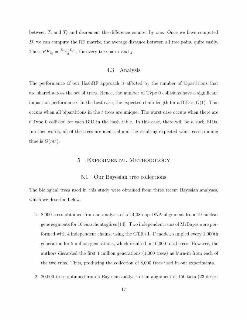
between Ti and Tj and decrement the difference counter by one. Once we have computed

D, we can compute the RF matrix, the average distance between all tree pairs, quite easily.

Thus, RF i,j = Di,j+Dj,i

2, for every tree pair i and j.

4.3 Analysis

The performance of our HashRF approach is affected by the number of bipartitions that

are shared across the set of trees. Hence, the number of Type 0 collisions have a significant

impact on performance. In the best case, the expected chain length for a BID is O(1). This

occurs when all bipartitions in the t trees are unique. The worst case occurs when there are

t Type 0 collision for each BID in the hash table. In this case, there will be n such BIDs.

In other words, all of the trees are identical and the resulting expected worst case running

time is O(nt2).

5 Experimental Methodology

5.1 Our Bayesian tree collections

The biological trees used in this study were obtained from three recent Bayesian analyses,

which we describe below.

1. 8,000 trees obtained from an analysis of a 14,085-bp DNA alignment from 19 nuclear

gene segments for 16 euarchontoglires [14]. Two independent runs of MrBayes were per-

formed with 4 independent chains, using the GTR+I+Γ model, sampled every 1,000th

generation for 5 million generations, which resulted in 10,000 total trees. However, the

authors discarded the first 1 million generations (1,000 trees) as burn-in from each of

the two runs. Thus, producing the collection of 8,000 trees used in our experiments.

2. 20,000 trees obtained from a Bayesian analysis of an alignment of 150 taxa (23 desert

17

taxa and 127 others from freshwater, marine, ands oil habitats) with 1,651 aligned

sites [15]. Two independent runs consisting of 25 million generations (trees were sam-

pled every 1,000 generations) were performed using the GTR+I+Γ model in MrBayes

with four independent chains. The authors constructed a majority consensus tree in

their study using the 20,000 trees from the last 10 million generations from each of the

two runs.

3. 33,306 trees obtained from an analysis of a three-gene, 567 taxa (560 angiosperms,

seven outgroups) dataset with 4,621 aligned characters, which is one of the largest

Bayesian analyses done to date [24]. Twelve runs, with four chains each, using the

GTR+I+Γ model in MrBayes ran for at least 10 million generations. Trees were sam-

pled every 1,000 generations. The authors discuss the difficulties with combining trees

from multiple runs. As a result, they decided to combine the trees from generations

7,372,000 – 10,160,000 that had a likelihood score of at least -238,050 to produce the

majority consensus tree and posterior probabilities. Only trees from 7 of the 12 runs

fit this criteria. For our experiments, in order to use the data from all 12 runs, the

trees from the first 8 million generations are discarded. This resulted in the 33,306

trees considered in our experiments.

In our experiments, for each number of taxa (n), we created different tree set sizes (t)

to test the scalability of the algorithms. Moreover, dividing the original tree collection into

smaller tree sets simulates using higher burn-in rates (i.e., higher burn-in rates means the

consensus tree is composed of fewer trees) as well as shorter Bayesian runs (fewer generations

produce fewer trees). For n = 16, the collection of 8, 000 trees is divided into smaller sets,

where t is 128, 256, 512, . . . , 4096 trees. The remaining datasets (n = 150 and 567) have

larger tree collections. Therefore, t ranges from 128 to 16,384 trees.

18

For each (n, t) pair, t trees with n taxa were randomly sampled without replacement

from the appropriate tree collection. For example, if n = 16, then t trees were selected

randomly from our entire collection of 8,000 trees. Trees with taxon sizes of 150 and 567

were sample from the collection of 20,000 and 33,306 trees, respectively. For each (n, t)

pair, we repeated the above sampling process five times. Our experimental results show the

average algorithmic performance for each (n, t) pair.

In Bayesian analyses, a majority tree is often computed from the sample of trees found

during the search. Figure 6(a) shows how the majority tree from all trees in the collection

differs from the majority tree created from t trees. The collection of 8, 000 trees for 16 taxa

are all identical. Hence, there is no impact on the resulting consensus tree when the original

tree collection is divided into smaller sub-collections of t trees. For the 150 and 567 taxa

datasets, the plot clearly shows that the majority tree created with t trees has on average

fewer than 4 different bipartitions than the majority tree created on the entire collections of

20,000 and 33,306 trees, respectively. In fact, the number average of bipartitions that differ

decrease as the number of trees, t, in the sub-collections increase. Thus, the quality of the

majority tree is not compromised by dividing the original tree collection into smaller sets of

t trees to study the performance of algorithms for summarizing tree collections.

Figure 6(b) plots the resolution rate of the majority consensus trees constructed from our

collection of t trees. The resolution rate of a phylogenetic tree is the number of bipartitions

contained in the tree divided by the number of bipartitions in a complete binary tree, which

is n − 3. A resolution rate of 100% represents a complete binary tree, and 0% corresponds

to a completely unresolved (or star) topology. Table 1 shows that the resolution rate of

the majority consensus tree for each of the original three tree collections is at least 85%.

However, the resolution of the strict consensus tree is much lower with a rate of up to 51%.

Figure 6(b) clearly shows that the resolution rate of the majority tree is very high (at

least 85%) for our smaller tree collections of size t datasets. The resolution of the majority

19

tree is unaffected by the increasing size of the tree collection. As expected, for the 150 and

567 taxa datasets, the resolution of the strict consensus tree decreases as the tree collection

size increases. Overall, the resolution rates of the consensus trees for our sub-collections

correspond with the resolution rates of the original, three tree collections.

5.2 Parameters for HashCS and HashRF algorithms

We pick a prime number to represent the size of our hash table, m1. Here, m1 is the smallest

prime number bigger than tn, the total number of bipartitions in the collection of trees.

For m2, which is used with our hash function h2, we choose the smallest prime number

larger than c · tn, where c is chosen to be 1,000. Thus, our algorithms have a 11000

or 0.1%

chance of producing an incorrect consensus tree or RF matrix. All experiments results were

compared across the competing algorithms (e.g., PAUP*, Phylip, Day) for experimental

validation. None of our runs of HashCS or HashRF during our experiments produced an

incorrect answer.

5.3 Consensus tree methods

We compare our HashCS algorithms to four different approaches: MrBayes, Phylip, PAUP*,

and Day’s algorithm. Day’s algorithm only computes the strict consensus tree as it cannot

be extended to compute majority trees. We do not explicitly compare the algorithms to TNT

it has been shown that PAUP* is much faster than TNT in constructing strict consensus

trees [4, 5, 13].

5.4 RF matrix methods

Our HashRF algorithm is compared to four different approaches: Phylip, PAUP*, Day’s

algorithm, and Pattengale, Gottlieb, and Moret’s Hashed (PGM-Hashed) algorithm [18].

20

Since some of the methods compute the full RF matrix (instead of the upper or lower

triangle), all algorithms compute the full matrix in our experiments. Both Phylip and PAUP*

actually compute the symmetric difference, but it can be transformed into the RF distance

by dividing this value by 2. In our experiments, we show the performance of computing the

symmetric difference in Phylip and PAUP*.

5.5 Implementations

All experiments were run on an Intel Pentium platform with a 3.0GHz processor and a total

of 2GB of memory. We also used the Linux operating system (Red Hat 2.5.22.14-17.fc6).

HashCS, HashRF, Day, and PGM-Hashed were written in C++ and compiled with gcc 4.1.2

with the -O3 compiler option. PAUP* is commercially available software and we used version

4.0b10 in our experiments. Phylip and MrBayes are freely available and we used software

versions 3.65 and 3.1.2, respectively.

6 Results

6.1 Consensus tree performance

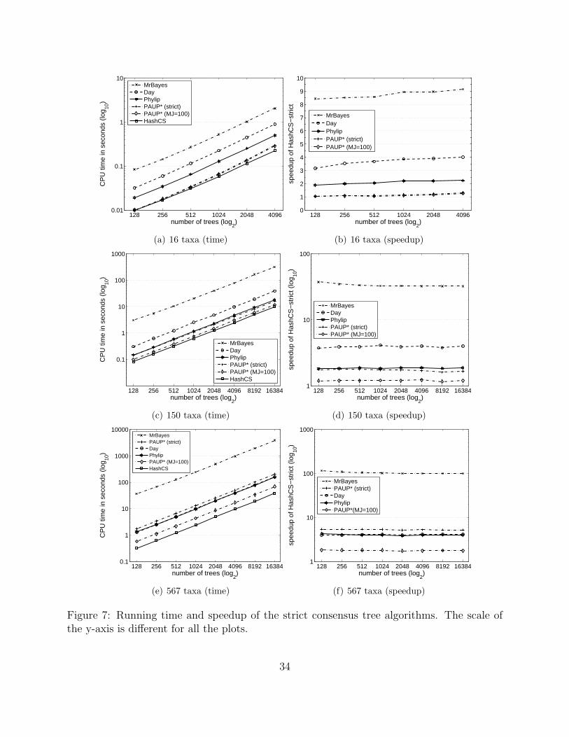
First, we consider the running time of our HashCS algorithm against its competitors for

computing the strict consensus tree. Figures 7(a), 7(c), and 7(e) show the results. Overall,

HashCS is the fastest algorithm for computing strict consensus trees. MrBayes is the slowest

approach requiring 1.1 hours compared to 38.3 seconds by HashCS on the largest dataset

(567 taxa, 16384 trees). Surprisingly, Day’s algorithm is not the fastest approach in practice

even though it is optimal from a theoretical complexity standpoint.

In our plots for Figure 7, we show two performance results for PAUP*. PAUP*(strict)

is the running time of the algorithm when using the strict command in the Nexus file.

PAUP*(MJ=100) computes the strict consensus tree, but using the majority option with

21

percent equal to 100%. Surprisingly, using the strict option takes considerably more time to

compute the same tree than using the majority option. The work of Boyer et al. observed

the same behavior [4, 5, 13]. In any case, PAUP*(MJ=100) is the second faster performer

behind HashCS.

Figures 7(b), 7(d), and 7(f) shows the speedup of the HashCS algorithm in comparison

to the other approaches. Speedup is calculated as xy, where x is the execution time required

by Day, MrBayes, PAUP*, or Phylip and y is the running time of HashCS. On the largest

dataset, HashCS is over 100 times faster than MrBayes and approximately 4 and 5 times

faster than Phylip and PAUP*, respectively. Figure 8 provides a closer look at the speedup of

the HashCS algorithm over its top competitor for constructing the strict consensus tree. The

plot clearly shows that the speedup of HashCS is unaffected by the size of the tree collection.

Instead, the performance of HashCS improves significantly with increasing number of taxa.

For majority trees, Figures 7(a), 7(c), and 7(e) clearly demonstrate HashCS and Mr-

Bayes are the fastest and slowest algorithms, respectively. The speedup of the HashCS

algorithm in comparison to the other majority approaches is shown in Figures 9(b), 9(d),

and 9(f). Again, HashCS’s performance increases significantly with larger taxa sizes. How-

ever, its performance is essentially unaffected by the number of trees in the collection (see

Figure 8(b)). For 567 taxa, HashCS computes a majority tree at least 60% faster than

PAUP*, its nearest competitor.

6.2 RF matrix performance

Figures 10(a), 10(c), and 10(e) shows the running time of the RF distance matrix algorithms.

Phylip and HashRF are the overall worst and best performers overall, respectively. In general,

much more time is required to compute the RF matrix than consensus trees. On the largest

dataset studied here, HashRF requires 1353.4 seconds (or 22.6 minutes). The only other

RF approach that was able to compute the RF matrix for this dataset was Day’s algorithm,

22

which required 13,123.4 seconds (or 3.64 hours). Both PAUP* and Phylip exceeded the time

limit of 12 hours to analyze this dataset.

Finally, the PGM-Hashed algorithm will not run this problem size either. PGM-Hashed

computes the probability of bipartitions colliding based on the number of taxa (n), number

of trees (t), and bitstring length (k = 64). If the collision probability exceeds a threshold

value, then the algorithm will not run the problem size as it is highly likely that the resulting

RF matrix will be incorrect.

Figures 10(b), 10(d), and 10(f) show the speedup of the HashRF approach over its

competitors. Speedup is calculated as xy, where x is the execution time required by PAUP*,

PGM-Hashed, and Phylip and y is the running time of HashRF. One trend of interest is

that the speedup of HashRF over PGM-Hashed, the second-best competitor, appears to be

decreasing with increasing number of trees. Figure 11(a) presents a more in-depth view of

the performance of these two algorithms. Clearly, the speedup of HashRF is decreasing with

increasing number of trees. Once the bipartitions have all been processed into the hash

table, the RF matrix can be calculated (step 2 of the algorithm). Figure 11(b) shows that

as the number of trees increases, up to 90% of the time can be consumed by step 2 of the

HashRF approach. For the datasets studied here, the majority consensus trees have over an

85% resolution rate. Since many of the bipartitions are shared across the trees, this results

in numerous Type 0 collisions in the hash table.

6.3 Weighted RF matrix performance

We can also compute the weighted RF distance, which takes into account the branch

lengths [21], of two trees. Suppose a bipartition B is common between two trees T1 and

T2. The weight (or branch length) of B in tree T1 is w1(B) and its weight in tree T2 is

w2(B). Thus, the weighted RF difference for bipartition B is |w1(B)−w2(B)|. To compute

the weighted RF distance between two trees T1 and T2, we would apply the above process

23

to all bipartitions in the two trees and sum the weighted difference between the bipartitions.

Moreover, we also need to handle appropriately those bipartitions that appear in only one

of the two trees.

Formally, suppose that every bipartition B in trees T1 and T2 has a positive branch length.

Let B ∈ Σ(T1) ∪ Σ(T2). w1(B) and w2(B) denote the length of the branch corresponding

to the bipartition B from Σ(T1) and Σ(T2), respectively. For all B ∈ Σ(T1) and B /∈ Σ(T2),

let w2(B) = 0. Similarly, let w1(B) = 0, for all B ∈ Σ(T2) and B /∈ Σ(T1). The weighted

Robinson-Foulds distance dw between trees T1 and T2 is then defined by

dw(T1, T2) =∑

B∈Σ(T1)∪Σ(T1)

|w1(B) − w2(B)|. (5)

The weighted RF distance matrix computes the weighted RF distance between every pair of

trees in the tree collection of size t. Of the algorithms studied here, only the weighted version

of our HashRF algorithm, which we call WHashRF algorithm, can compute the t×t weighted

RF matrix. The biggest difference between WHashRF and HashRF is that WHashRF must

also keep track of the branch length associated with each bipartition B from tree T into the

hash table .

Figure 12 shows the distribution of the unweighted and weighted RF distance values for

our collection of 150 and 567 taxa trees. For the unweighted RF distance, branch lengths are

assumed to be one. However, the actual branch lengths returned by the Bayesian analysis

have values much smaller than one. Although the weighted RF matrix may prove to be

more useful for some datasets (e.g., as in the case of the identical 16 taxon trees), computing

the weighted RF matrix does require more time than its unweighted counterpart. Figure 13

shows that the HashRF algorithm is up to 5 times faster than WHashRF algorithm.

24

7 Conclusions

In this paper, we introduce the HashCS and HashRF algorithms as fast techniques for

summarizing evolutionary relationships contained in a set of phylogenetic trees. The novelty

of the HashCS and HashRF algorithms is our use of hash tables, which provides a convenient

and fast approach to store and access the relationships depicted in the tree collections. Hash

tables have been widely used to develop extremely fast bioinformatics algorithms such as

BLAST [1] and FASTA [19] for comparing molecular sequences. Our work extends the use

of hash tables in bioinformatics to summarizing phylogenetic trees quickly.

Our hash-based algorithms provide a general approach for summarizing tree collections

quickly. In particular, HashCS is up to 80% faster than PAUP*, the second fastest consensus

algorithm. For our HashRF algorithm, it is up to 3 times faster than its closest competitor,

PGM-Hashed. HashRF is several orders faster than Day, PAUP*, and Phylip. Moreover,

HashRF requires less time to compute a distance matrix than MrBayes requires for comput-

ing a consensus tree. Finally, we show that there is a performance penalty for computing the

weighted versus unweighted RF distance matrix. However, our WHashRF algorithm com-

putes the weighted RF matrix much faster than the other competing RF algorithms (except

PGM-Hashed) calculate an unweighted RF distance matrix.

Fast algorithms such as HashCS and HashRF make it feasible to study the relationships

contained in a collection of trees in a reasonable amount of time. Much attention has been

placed on speeding up phylogenetic search algorithms. However, other techniques (such as

summarization algorithms) must be scaled up as well to meet the challenge of reconstructing

the Tree of Life. For example, the work of Hillis et al. showed the potential for comparing two

different Bayesian analyses consisting of 44-taxon trees using multidimensional scaling, where

they used a matrix of RF tree distances as input [11]. However, with existing RF software

it would have been infeasible to compare larger collections of Bayesian trees. As the size

25

and number of trees increases, our results demonstrate that our HashRF software runs in

seconds or minutes compared to hours or even days with PAUP* or Phylip. Moreover, with

the HashCS and HashRF algorithms, it becomes possible to consider real-time summaries of

tree collections formed during a phylogenetic analysis. Thus, our fast hash-based algorithms

allow systematics to study their collections of trees in new and exciting ways.

8 Acknowledgments

The authors wish to thank Nick Pattengale, Eric Gottlieb, and Bernard Moret for providing

the code for Day’s algorithm as well as the code for their PGM-Hashed RF distance matrix

algorithm. We would also like to thank Matthew Gitzendanner, Bill Murphy, Paul Lewis,

and David Soltis for providing us with the Bayesian tree collections used in this paper.

Finally, we thank Tandy Warnow for her very helpful comments during the preparation of

this manuscript. Funding for this project was supported by the National Science Foundation

under grants DEB-0629849 and IIS-0713618.

References

[1] S. Altschul, W. Miller, E. Myers, and D. Lipman. Basic local alignment search tool. J

Mol Biol, 215(3):403–410, 1990.

[2] N. Amenta, F. Clarke, and K. S. John. A linear-time majority tree algorithm. In

Workshop on Algorithms in Bioinformatics, volume 2168 of Lecture Notes in Computer

Science, pages 216–227, 2003.

[3] O. R. P. Bininda-Emonds. MRP supertree construction in the consensus setting. In

M. Janowitz, F. Lapointe, F. McMorris, B. Mirkin, and F. Roberts, editors, Biocon-

26

sensus, DIMACS Series in Discrete Mathematics and Theoretical Computer Science.

DIMACS-AMS, 2001.

[4] R. S. Boyer, W. A. Hunt Jr., and S. Nelesen. A compressed format for collections of

phylogenetic trees and improved consensus performance. Technical Report TR-05-12,

Department of Computer Sciences, The University of Texas at Austin, 2005.

[5] R. S. Boyer, W. A. Hunt Jr., and S. Nelesen. A compressed format for collections of

phylogenetic trees and improved consensus performance. In Proc. 5th Int’l Workshop

Algorithms in Bioinformatics (WABI’05), volume 3692 of Lecture Notes in Computer

Science, pages 353–364. Springer-Verlag, 2005.

[6] D. Bryant. A classification of consensus methods for phylogenetics. In M. Janowitz,

F. Lapointe, F. McMorris, B. Mirkin, and F. Roberts, editors, Bioconsensus, volume 61

of DIMACS: Series in Discrete Mathematics and Theoretical Computer Science, pages

163–184. American Mathematical Society, DIMACS, 2003.

[7] W. H. E. Day. Optimal algorithms for comparing trees with labeled leaves. Journal Of

Classification, 2:7–28, 1985.

[8] J. Felsenstein. Phylogenetic inference package (PHYLIP), version 3.2. Cladistics, 5:164–

166, 1989.

[9] L. R. Foulds and R. L. Graham. The Steiner problem in phylogeny is NP-complete.

Advances in Applied Mathematics, 3:43–49, 1982.

[10] P. Goloboff. Analyzing large data sets in reasonable times: solutions for composite

optima. Cladistics, 15:415–428, 1999.

[11] D. M. Hillis, T. A. Heath, and K. S. John. Analysis and visualization of tree space.

Syst. Biol, 54(3):471–482, 2005.

27

[12] J. P. Huelsenbeck and F. Ronquist. MRBAYES: Bayesian inference of phylogenetic

trees. Bioinformatics, 17(8):754–755, 2001.

[13] W. A. Hunt Jr. and S. M. Nelesen. Phylogenetic trees in ACL2. In Proc. 6th Int’l Conf.

on ACL2 Theorem Prover and its Applications (ACL2’06), pages 99–102, New York,

NY, USA, 2006. ACM.

[14] J. E. Janecka, W. Miller, T. H. Pringle, F. Wiens, A. Zitzmann, K. M. Helgen, M. S.

Springer, and W. J. Murphy. Molecular and genomic data identify the closest living

relative of primates. Science, 318:792–794, 2007.

[15] L. A. Lewis and P. O. Lewis. Unearthing the molecular phylodiversity of desert soil

green algae (chlorophyta). Syst. Bio., 54(6):936–947, 2005.

[16] W. J. Murphy, E. Eizirik, S. J. O’Brien, O. Madsen, M. Scally, C. J. Douady, E. Teeling,

O. A. Ryder, M. J. Stanhope, W. W. de Jong, and M. S. Springer. Resolution of the

early placental mammal radiation using bayesian phylogenetics. Science, 294:2348–2351,

2001.

[17] K. C. Nixon. The parsimony ratchet, a new method for rapid parsimony analysis.

Cladistics, 15:407–414, 1999.

[18] N. Pattengale, E. Gottlieb, and B. Moret. Efficiently computing the Robinson-Foulds

metric. Journal of Computational Biology, 14(6):724–735, 2007.

[19] W. Pearson and D. Lipman. Improved tools for biological sequence comparison. PNAS,

85(8):2444–8, 1988.

[20] K. Rice, M. Donoghue, and R. Olmstead. Analyzing large datasets: rbcL 500 revisited.

Systematic Biology, 46(3):554–563, 1997.

28

[21] D. Robinson and L. Foulds. Comparison of weighted labelled trees. In Proc. Sixth

Austral. Conf., volume 748 of Lecture Notes in Mathematics, pages 119–126. Springer-

Verlag, 1979.

[22] U. Roshan. Detailed experimental results on the performance of Rec-I-

DCM3 as presented in CSB’04. Internet Website, last accessed, Nov 2005.

http://www.cs.njit.edu/usman/dcm3/recidcm3 csb04 data.html.

[23] D. Sikes and D. O. Lewis. PAUPRat: PAUP implementation of the parsimony ratchet,

2001. http://www.ucalgary.ca/ dsikes/software2.htm.

[24] D. E. Soltis, M. A. Gitzendanner, and P. S. Soltis. A 567-taxon data set for an-

giosperms: The challenges posed by bayesian analyses of large data sets. Int. J. Plant

Sci., 168(2):137–157, 2007.

[25] T. A. Standish. Data structures techniques. Addison-Wesley, 1980.

[26] C. Stockham, L. S. Wang, and T. Warnow. Statistically based postprocessing of phylo-

genetic analysis by cluste ring. In Proceedings of 10th Int’l Conf. on Intelligent Systems

for Molecular Biology (ISMB’02), pages 285–293, 2002.

[27] S.-J. Sul and T. L. Williams. A randomized algorithm for comparing sets of phylogenetic

trees. In Proc. Fifth Asia Pacific Bioinformatics Conference (APBC’07), pages 121–130,

2007.

[28] D. L. Swofford. PAUP*: Phylogenetic analysis using parsimony (and other methods),

2002. Sinauer Associates, Underland, Massachusetts, Version 4.0.

29

B

A C D

E

T1

B

A D C

E

T2

B

A E C

D

T3

E

A B D

C

T4

T 1T 2 T 3 T 4

1

1

1 2

2

1

T 1

T 2

T 3

T 4

I n p u t T r e e s

R F D i s t a n c e M a t r i x

B

A C

D

EB

A C

D

E

M a j o r i t y C o n s e n s u sT r e e

S t r i c t C o n s e n s u sT r e e

1

1

2 2

1

1 0

0

0

0

B 2B 1 B 3 B 4 B 5 B 6 B 7 B 8

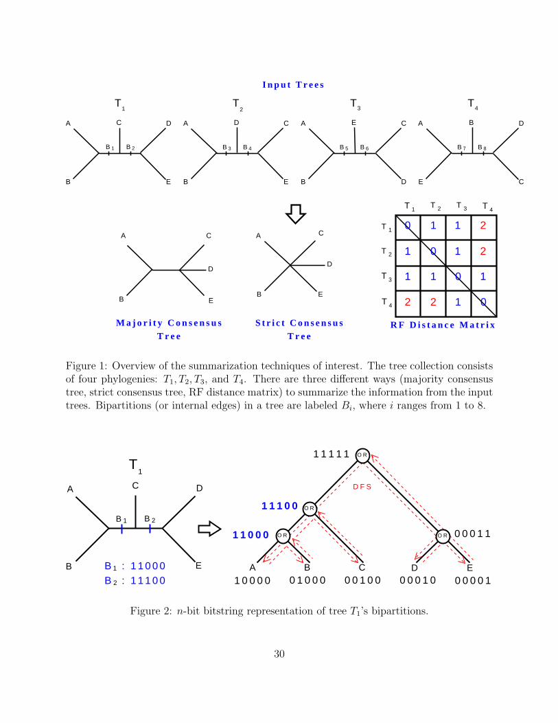
Figure 1: Overview of the summarization techniques of interest. The tree collection consistsof four phylogenies: T1, T2, T3, and T4. There are three different ways (majority consensustree, strict consensus tree, RF distance matrix) to summarize the information from the inputtrees. Bipartitions (or internal edges) in a tree are labeled Bi, where i ranges from 1 to 8.

B

A C D

E A B C D E1 0 0 0 0 0 1 0 0 0 0 0 1 0 0 0 0 0 1 0 0 0 0 0 1

1 1 0 0 0

1 1 1 0 0

0 0 0 1 1

1 1 1 1 1

D F S

B : 1 1 0 0 0B : 1 1 1 0 0

1

2

O R

O R

O R

O R

T1

B 1 B 2

Figure 2: n-bit bitstring representation of tree T1’s bipartitions.

30

0

4

8

4 6

3 1

2 7

. . .

3 5

1

3

1

1

m - 11

1 7

...

4 02

h1

1

2

3

T Y P E 1 c o l l s i o n

T1

T2

T3

7B7B

6B

5B

4B

3B

2B

1B

T48BB

H a s h T a b l eB i p a r t i t i o n s H a s h R e c o r d s

Figure 3: Overview of the HashCS algorithm. Bipartitions are from Figure 1. That is, B1

and B2 define T1, B3 and B4 are from T2, etc. The implicit representation of each bipartitionis fed to the hash functions h1 and h2. The shaded value in each hash record containsthe bipartition ID (or h2 value) whereas the unshaded value shows the frequency of thatbipartition.

Number of Size of tree strict resolution majority resolutiontaxa collection rate rate16 8,000 100% 100%150 20,000 34% 87%567 33,603 51% 93%

Table 1: Resolution rates of consensus trees of our entire tree collections.

31

6

n-b i t

b i p a r t i t i o n

0 1 0 0 0

2 1

0 0 1 0 0

1 0

0 0 0 1 0

8

0 0 0 0 1

1 9

1 1 1 1 1

1 8

1 1 0 0 0

4

1 1 1 0 0

1 4

0 0 0 1 1

4

1 0 0 0 0

U V W X Y

N 5

N3 N 8

N9

T r e e T

N1 N2 N4 N6 N7

h v a l u e1

Figure 4: Calculating the h1 hash code from n-bitstring bipartitions representations basedon a postorder traversal of an example tree T . Each node is labeled by Ni, where i is theorder in which it was visited during the postorder traversal. The input taxa are U, V,W,X,and Y and are represented by nodes N1, N2, N4, N6, and N7, respectively. To compute the h1

hashing function, m1 = 23 and the contents of array R are r0 = 6, r1 = 21, r2 = 10, r3 = 8,and r4 = 19. Each node in the tree T shows an n-bitstring representation (shaded) alongwith the corresponding h1 value (unshaded). The h1 values of the nodes are computed basedon Equations 2 and 5. For node N5, h1(11100) = (1·r0+1·r1+1·r2+0·r3+0·r4) mod 23 = 14.

32

H a s h T a b l e

0

4

8

...

m - 11

1 7

...

h1

B i p a r t i t i o n s

1

2

3

T1

T2

T3

7B7B

6B

5B

4B

3B

2B

1B

T48B

T Y P E 0 c o l l s i o n s

T Y P E 1 c o l l s i o n

H a s h R e c o r d s

T1

2 7 3 5

T1 T2 T3 T4

3 1

4 0

T2

T3 T4 T Y P E 0 c o l l s i o n s

4 6

Figure 5: Overview of the HashRF algorithm. Bipartitions are from Figure 1. The implicitrepresentation of each bipartition is fed to the hash functions h1 and h2. The shaded valuein each hash record contains the bipartition ID (or h2 value). Each bipartition ID has alinked list of tree indexes that share that particular bipartition.

128 256 512 1024 2048 4096 8192 163840

0.5

1

1.5

2

2.5

3

3.5

4

4.5

5

number of trees (log2)

RF

dis

tanc

e

150 taxa567 taxa16 taxa

(a) RF distance

128 256 512 1024 2048 4096 8192 1638430

40

50

60

70

80

90

100


aver

age

reso

lutio

n ra

te (

%)

16 taxa (majority)16 taxa (strict)567 taxa (majority)150 taxa (majority)567 taxa (strict)150 taxa (strict)

(b) Resolution rate

Figure 6: Comparison of consensus trees. (a) The average RF distance between the overallmajority consensus tree and the majority consensus composed of t trees. (b) Average res-olution rate of the consensus trees constructed from our Bayesian tree collections. The 16taxa trees are all identical which leads to a 100% resolution rate of the consensus trees.

33

128 256 512 1024 2048 40960.01

0.1

1

10


CP

U ti

me

in s

econ

ds (

log 10

)

MrBayesDayPhylipPAUP* (strict)PAUP* (MJ=100)HashCS

(a) 16 taxa (time)

128 256 512 1024 2048 40960

1

2

3

4

5

6

7

8

9

10


spee

dup

of H

ashC

S−

stric

t

MrBayesDayPhylipPAUP* (strict)PAUP* (MJ=100)

(b) 16 taxa (speedup)

128 256 512 1024 2048 4096 8192 16384

0.1

1

10

100

1000


CP

U ti

me

in s

econ

ds (

log 10

)

MrBayesDayPhylipPAUP* (strict)PAUP* (MJ=100)HashCS

(c) 150 taxa (time)

128 256 512 1024 2048 4096 8192 163841

10

100


spee

dup

of H

ashC

S−

stric

t (lo

g 10)

MrBayesDayPhylipPAUP* (strict)PAUP* (MJ=100)

(d) 150 taxa (speedup)

128 256 512 1024 2048 4096 8192 163840.1

1

10

100

1000

10000


CP

U ti

me

in s

econ

ds (

log 10

)

MrBayesPAUP* (strict)DayPhylipPAUP* (MJ=100)HashCS

(e) 567 taxa (time)

128 256 512 1024 2048 4096 8192 163841

10

100

1000


spee

dup

of H

ashC

S−

stric

t (lo

g 10)

MrBayesPAUP* (strict)DayPhylipPAUP*(MJ=100)

(f) 567 taxa (speedup)

Figure 7: Running time and speedup of the strict consensus tree algorithms. The scale ofthe y-axis is different for all the plots.

34

128 256 512 1024 2048 4096 8192 163841

1.1

1.2

1.3

1.4

1.5

1.6

1.7

1.8

1.9

2


spee

dup

of H

ashC

S−

stric

t


(a) strict consensus

128 256 512 1024 2048 4096 8192 163840.8

0.9

1

1.1

1.2

1.3

1.4

1.5

1.6

1.7

1.8


spee

dup

of H

ashC

S−

maj

ority


(b) majority consensus

Figure 8: Speedup of the HashCS algorithm over PAUP*, its top consensus tree competitor.(a) Speedup of HashCS over PAUP* to compute the strict consensus tree. (b) Speedup ofHashCS over PAUP* to compute the majority tree. The scale of the y-axis is different forall the plots.

35

128 256 512 1024 2048 40960.01

0.1

1

10


CP

U ti

me

in s

econ

ds (

log 10

)

MrBayesPhylipPAUP*HashCS

(a) 16 taxa (time)

128 256 512 1024 2048 40960

1

2

3

4

5

6

7

8

9

10


spee

dup

of H

ashC

S−

maj

ority

MrBayesPhylipPAUP*


128 256 512 1024 2048 4096 8192 16384

0.1

1

10

100

1000


CP

U ti

me

in s

econ

ds (

log 10

)


(c) 150 taxa (time)

128 256 512 1024 2048 4096 8192 163841

10

100


spee

dup

of H

ashC

S−

maj

ority

(lo

g 10)

MrBayesPhylipPAUP*


128 256 512 1024 2048 4096 8192 163840.1

1

10

100

1000

10000


CP

U ti

me

in s

econ

ds (

log 10

)


(e) 567 taxa (time)

128 256 512 1024 2048 4096 8192 163841

10

100

1000


spee

dup

of H

ashC

S−

maj

ority

(lo

g 10)

MrBayesPhylipPAUP*


Figure 9: Running time and speedup of the majority consensus tree algorithms. The scaleof the y-axis is different for all the plots.

36

128 256 512 1024 2048 40960.01

0.1

1

10

100

1000


CP

U ti

me

in s

econ

ds (

log 10

)

PhylipPAUP*DayPGM−HashedHashRF

(a) 16 taxa (time)

128 256 512 1024 2048 40960

10

20

30

40

50

60


spee

dup:

oth

ers

/ Has

hRF

PhylipPAUP*DayPGM−Hashed


128 256 512 1024 2048 4096 8192 163840.1

1

10

100

1000

10000

100000


CP

U ti

me

in s

econ

ds (

log 10

)


(c) 150 taxa (time)

128 256 512 1024 2048 4096 8192 163841

10

100

1000

10000


spee

dup

of H

ashR

F (

log 10

)



128 256 512 1024 2048 4096 8192 163840.1

1

10

100

1000

10000

100000


CP

U ti

me

in s

econ

ds (

log 10

)


(e) 567 taxa (time)

128 256 512 1024 2048 4096 8192 163841

10

100

1000

10000

100000


spee

dup

of H

ashR

F (

log 10

)



Figure 10: Running time and speedup of the RF distance matrix algorithms. Data pointsfor Phylip and PAUP* are missing if computation time exceeded 12 hours. Data points forPGM-Hashed are missing if it couldn’t run that problem size. The scale of the y-axis isdifferent for all the plots.

37

128 256 512 1024 2048 4096 8192 163841

1.5

2

2.5

3

3.5


spee

dup

of H

ashR

F o

ver

PG

M−

Has

hed 150 taxa

567 taxa16 taxa

(a) Speedup of HashRF over PGM-Hashed

128 256 512 1024 2048 4096 8192 163840

10

20

30

40

50

60

70

80

90

100


com

pute

mat

rix ti

me

/ tot

al ti

me

(%)


(b) percentage of time for step 2 in HashRF

Figure 11: A closer view at the performance of HashRF. (a) Speedup of HashRF over PGM-Hashed. (b) Percentage of time HashRF spends calculating the RF matrix once all thebipartitions are in the hash table (i.e., step 2 of the algorithm).

38

128 256 512 1024 2048 4096 8192 163845

10

15

20

25

30

35

40

45

50

55

unw

eigh

ted

RF

dis

tanc

e

number of trees

(a) 150 taxa (unweighted)

128 256 512 1024 2048 4096 8192 16384

0.5

0.6

0.7

0.8

0.9

1

1.1

1.2

1.3

wei

ghte

d R

F d

ista

nce

number of trees

(b) 150 taxa (weighted)

128 256 512 1024 2048 4096 8192 163840

20

40

60

80

100

120

unw

eigh

ted

RF

dis

tanc

e

number of trees

(c) 567 taxa (unweighted)

128 256 512 1024 2048 4096 8192 16384

0.2

0.4

0.6

0.8

1

1.2

1.4

1.6

1.8

2

wei

ghte

d R

F d

ista

nce

number of trees

(d) 567 taxa (weighted)

Figure 12: Distribution of unweighted and weighted RF distances for the 150- and 567-taxondatasets. Since all of the 16-taxon trees are identical, the unweighted RF distance betweenall trees is 0. However, the weighted RF distance ranged from 0.005 to 0.05. The scale ofthe y-axis is different for all the plots.

39

128 256 512 1024 2048 4096 8192 163840

1

2

3

4

5

6


spee

dup

of H

ashR

F o

ver

WH

ashR

F


Figure 13: Speedup of unweighted HashRF over weighted HashRF.

40

Documents

Fast Hashing Algorithms to Summarize Large Collections · PDF fileTexas A&M CS Technical Report 2008-6-1 June 27, 2008 Fast Hashing Algorithms to Summarize Large Collections of Evolutionary