Embed Size (px)
Citation preview

1
FAST PHYSICS–BASED METHODS FOR WIDEBAND ELECTROMAGNETIC INDUCTION DATA ANALYSIS
By
GANESAN RAMACHANDRAN
A DISSERTATION PRESENTED TO THE GRADUATE SCHOOL OF THE UNIVERSITY OF FLORIDA IN PARTIAL FULFILLMENT
OF THE REQUIREMENTS FOR THE DEGREE OF DOCTOR OF PHILOSOPHY
UNIVERSITY OF FLORIDA
2010

2
© 2010 Ganesan Ramachandran

3
ACKNOWLEDGMENTS
I thank my mother, JothiSree Venkataraman; father, Ramachandran Sethunarayanan; and
wife, Swetha Seetharaman, for their relentless love and support.
I thank my advisor, Paul Gader, for his guidance and encouragement throughout my tenure
at the University of Florida. I thank my committee Paul Gader, Joseph Wilson, Arunava
Banerjee, and John Harris for their insight and guidance which has steered my research and
bettered resulting contributions.
I thank my lab mates for their support and am thankful for their ability to endure my
shenanigans. I thank Andres Mendez-Vasquez, Seniha Esen Yuksel, Xuping Zhang and
Gyeongyong Heo for their encouragement, suggestions and aid in my research.
I thank colleagues, Jim Keller, Hichem Frigui, Peter Torrione and Dominic Ho, for their
collaboration on a variety of research projects.
I thank Russell Harmon of Army Research Office (ARO), Richard Weaver and Mark
Locke of Night Vision and Electronic Sensors Directorate (NVESD), and Waymond Scott of
Georgia Tech, for their support of my research.

4
TABLE OF CONTENTS page
ACKNOWLEDGMENTS ...............................................................................................................3
LIST OF TABLES ...........................................................................................................................6
LIST OF FIGURES .........................................................................................................................7
ABSTRACT .....................................................................................................................................9
1 INTRODUCTION ..................................................................................................................11
Wideband Electromagnetic Induction Data and Analysis ......................................................11 Statement of Problem .............................................................................................................12 Overview of Research .............................................................................................................12
2 LITERATURE REVIEW .......................................................................................................14
Induced Field of a Homogeneous Sphere ...............................................................................14 Spectral Models ......................................................................................................................17
Bell-Miller Models ..........................................................................................................17 First order Cole-Cole model .....................................................................................19 Nonlinear least squares optimization .......................................................................21 Bishay’s circle fitting method ..................................................................................21 Xiang’s direct inversion method ..............................................................................23 Bayesian inversion ...................................................................................................24
Discrete Spectrum of Relaxation Frequencies ................................................................24 Kth Order Cole-Cole ........................................................................................................26
3 TECHNICAL APPROACH ...................................................................................................27
Argand Diagrams of WEMI Responses .................................................................................28 Prototype Angle Matching ......................................................................................................29 Gradient Angle Model Algorithm ..........................................................................................30
Stability of Lookup Table Step in GRANMA .................................................................32 Classifier Design .............................................................................................................34
Gradient Angles in Parts Algorithm .......................................................................................34 Filter Design ....................................................................................................................36 Classifier Design .............................................................................................................37
Dielectric Relaxation estimation using Sparse Models ..........................................................37 Non-negative Least Squares Optimization ......................................................................38 Convex Optimization with Sparsity Constraint ...............................................................38
Quadratic programming ...........................................................................................40 Linear programming .................................................................................................41
Joint Sparse Estimation of Dielectric Relaxations ..................................................................42 Gradient Newton Methods ..............................................................................................44

5
Lp,q Regularized Optimization ..................................................................................44 Iterative Reweighted Optimization ..........................................................................46 L1 Optimization ........................................................................................................47
Dictionary Learning using Adaptive Kernels ..................................................................49 Double Dictionary Search ...............................................................................................51
4 RESULTS ...............................................................................................................................53
Comparison on Synthetic Data ...............................................................................................53 Experiment 1: Data from first order model .....................................................................53 Observations ....................................................................................................................54 Experiment 2: Comparison of Joint Sparse Methods on Data from second order
model............................................................................................................................56 Experiment 3: Comparison of Cole-Cole and DSRF Dictionaries ..................................58 Experiment 4: Dictionary update .....................................................................................60 Experiment 5: Double Dictionary search – Proof of concept ..........................................61 Experiment 6: Dictionary Correlation Analysis ..............................................................63
Comparison on Landmine Data ..............................................................................................64 Data Sets ..........................................................................................................................64 Data Filtering ...................................................................................................................65 Experiment 6: Classification of objects using first order model .....................................65
Experiment setup ......................................................................................................65 Experiments and observations ..................................................................................66 PRAM analysis .........................................................................................................66 GRANMA analysis ..................................................................................................66 Bishay method and Xiang inversion analysis ..........................................................68
Feature Selection .............................................................................................................68 Observations ....................................................................................................................68 Experiment 7: Analysis of GRANPA on landmine data .................................................69 Experiment 8: Analysis of Dictionary methods on landmine data ..................................72
5 CONCLUSIONS ....................................................................................................................76
LIST OF REFERENCES ...............................................................................................................77
BIOGRAPHICAL SKETCH .........................................................................................................79

6
LIST OF TABLES
Table page 4-1 Comparison of convergence statistics: Part (1). ................................................................59
4-2 Comparison of convergence statistics: Part (2) .................................................................60
4-3 Nomenclature and Proportion ............................................................................................64

7
LIST OF FIGURES
Figure page 2-1 Pictorial representation of the data collection setup ..........................................................14
2-2 Geometry terms gn(r,dT,dS,RT,RS) for n from 1 to 4. ...........................................................16
2-3 Shape terms χn(kr) for n from 1 to 4. ................................................................................16
2-4 Effect of varying τ and α. ..................................................................................................20
2-5 Real vs. imaginary parts of data from a first order Cole-Cole model. ...............................22
2-6 Effect of pole spread on DSRF coefficients. .....................................................................25
3-1 Argand plots of WEMI response. ......................................................................................28
3-2 Angle plots of WEMI response. .........................................................................................30
3-3 Plot of gradient angle m in degrees ....................................................................................33
3-4 A) ∂m/∂τ and B) ∂m/∂α of the proposed model ................................................................33
3-5 Argand diagram of a low metal Anti-Personnel mine in the near field. ............................35
3-7 Estimated relaxations A) τ=10-5, B) τ=10-4 and C) τ=10-3.4. .............................................52
4-1 Real vs Imaginary part of the induced response of a sample. ............................................53
4-2 Fitting Error vs. Signal Energy for different parameter estimation methods ....................55
4-3 Actual vs. estimated parameter values for noise free case. ................................................55
4-4 Actual vs. estimated parameter values for ρ = 10-4. ..........................................................56
4-5 Histogram image of Number of terms vs. Fitting error .....................................................57
4-6 Convergence diagnostics for dictionary search and update. ..............................................61
4-8 Two nonzero rows of the weight matrix WT. .....................................................................62
4-9 Correlation regions of a Cole-Cole dictionary region.. ......................................................63
4-10 Down-track filter template .................................................................................................65
4-11 Plot showing the relationship between τ, α and EL for different mine types. ....................66
4-12 τ and α for different object types. ......................................................................................67

8
4-13 ROC curves of different landmine detection algorithms. ..................................................69
4-14 Change in Argand diagram with distance. .........................................................................69
4-15 Change in amplitude with distance ....................................................................................70
4-18 Parameter values estimated using joint sparse DSRF along down-track. ..........................73
4-19 Relaxations estimated using a Cole-Cole dictionary .........................................................74
4-20 Usage of dictionary elements by the landmine data.. ........................................................74
4-21 Entropy of estimated relaxations for 28 different mine types. ...........................................75

9
Abstract of Dissertation Presented to the Graduate School of the University of Florida in Partial Fulfillment of the Requirements for the Degree of Doctor of Philosophy
FAST PHYSICS–BASED METHODS FOR WIDEBAND ELECTROMAGNETIC
INDUCTION DATA ANALYSIS
By
Ganesan Ramachandran
May 2010 Chair: Paul Gader Major: Electrical and Computer Engineering
Three methods of object recognition using wideband electromagnetic induction data are
described. A fourth method, which extends an existing algorithm to extract features using a
dictionary based search, was developed to analyze objects. Emphasis was given to speed of
execution as our interest is in their real-time performance.
Wideband electromagnetic induction data may consist of a wide range of frequencies
starting from a few Hz to a few hundred thousand Hz. In addition to the object, the data usually
has information about the sensor geometry, orientation of data collection setup and the medium
in which the object lies.
The first method is called the Prototype Angle Matching (PRAM) algorithm that takes a
non-parametric approach using the gradient angle between the real and imaginary components of
the data. It classifies using distance from prototypes whose gradient angles have been measured.
It is fast and does not make any assumptions about the data.
The second method, the Gradient Angle Model Algorithm (GRANMA), is based on a
novel analytical derivation of the gradient angle using a first order Cole-Cole model. The
analytical derivation reduces the number of parameters from four to two, enabling a fast look-up
approach to nearest-neighbor classification schemes. Furthermore, the other two parameters can

10
easily be estimated from the first two. The method is demonstrated to be much faster and more
robust than existing methods.
The third method, Gradient Angles in Parts Algorithm (GRANPA) uses a piecewise Cole-
Cole modeling approach to attempt to estimate parameters of higher order models. It estimates
the frequency segments in the data that follow the Cole-Cole model in an automated way and
then uses the same setup as the GRANMA to extract the parameters.
The fourth set of methods, collectively referred to as SPARse DIelectric Relaxation
estimation (SPARDIR), use a model that generalizes the Discrete Spectrum of Relaxation
Frequencies (DSRF) model. The SPARDIR algorithms assume that the data are formed by a
weighted combination of the Cole-Cole models and use a gradient Newton framework to search
for parameters. A variety of combinations of L1 and L2 norm-based objective functions and
constraints are investigated to seek sparse, physically meaningful parameter estimates.
Furthermore, SPARDIR algorithms are devised that perform joint sparse estimation of
parameters over a set of measurements and compared to SPARDIR and DSRF algorithms that
perform point-wise sparse estimation.
Classification and parameter estimation results are given on sets of real, measured data as
well as synthetic data sets for which the true parameter values are known. In these experiments,
GRANMA performed better, more robust and with higher classification rates, than several
existing algorithms and is faster than all but one. The Joint SPARDIR algorithms more
accurately estimated the true underlying model parameters for more general models than
previous work. In addition, the Joint SPARDIR algorithms are general; they are not specific to
sensor type.

11
CHAPTER 1 INTRODUCTION
Wideband Electromagnetic Induction Data and Analysis
Wideband electromagnetic induction (WEMI) sensors have been used in a wide variety of
applications ranging from finding mineral ore deposits [1] to monitoring blood glucose levels
[2]. They are mainly divided into time domain and frequency domain sensors based on the
domain of interpretation. The time domain sensors operate on the principle that when a time
varying electrical current from a primary transmitter is injected through a dielectric medium, part
of the electrical power is stored in the medium. When the current is stopped, the stored energy
dissipates. This energy dissipation creates a secondary electric field which can be measured by a
receiver. The rate at which the energy dissipates depends on the dielectric properties of the
medium. This phenomenon is known as induced polarization (IP) [3].
Frequency domain sensors use a discrete number of sinusoidal signals. The secondary
electric field or the induced field differs from the primary in amplitude and phase. This can be
represented as the result of change in the complex impedance of the sensor [4]. By having the
primary field consist a wide range of frequencies, we can get a complex spectral signature of the
object under investigation. The main appeal of using electromagnetic induction is that different
materials have different spectral signatures that can be used to detect and identify them. Also,
different materials have different bandwidths, i.e., frequencies at which they produce maximum
induction response.
There exists a multitude of electromagnetic induction sensors or metal detectors as they are
more commonly known. Some commercial handheld metal detectors use a small range of
frequencies and have applications such as treasure hunting or airport security. Their designs vary
in the bandwidth of interest for the minerals they are tuned for. Most of them use the energy in

12
the secondary field for detection and seldom have discrimination capabilities between different
materials within same bandwidth.
Wideband EMI sensors, as their name indicates, use a wide range of frequencies to identify
different liquids or solids. Their frequencies of operation can range from a few hundreds of Hz to
a few KHz. They are used in a variety of applications such as mineral prospecting, biological
tissue analysis and landmine detection.
Statement of Problem
Parametric models offer a framework for characterization and classification of different
objects in a physically interpretable way. Most parametric models for wideband EMI data are
based on simplifications of Maxwell’s equations to characterize the secondary field. But they
often suffer from one or more of the following assumptions
• The object to be identified is suspended in vacuum • The object comprises of a single homogeneous material • The object is of a simple geometric shape (sphere, cylinder etc) • The surrounding medium is magnetically transparent • Non-targets or clutter can be modeled
Even though most parametric models make such assumptions, they are still highly
nonlinear. Parameter estimation is a nontrivial problem in most cases. Also most algorithms use
iterative methods that require good knowledge of search ranges and starting values. We need
models that are reasonably accurate to fit the observed data and estimated parameters to be
consistent for identical objects to enable classification. Also, we need parameter estimation
methods that are fast enough to be employed in practical applications.
Overview of Research
This research involved the development and analysis of both parametric and nonparametric
models to detect, analyze and identify different metallic objects using frequency domain

13
wideband EMI sensors. The primary objective was to develop fast, physics-based algorithms for
landmine detection and extend them to other applications. We first developed models to
characterize spectral shapes at a given location and then modeled the variation in the parameters
with respect to distance and orientation of the sensor from the object.
The first method uses only the shape information in the spectral signature and designs a
prototype matching framework. It is nonparametric and hence does not make any assumptions
about the data distribution. It creates a fast anomaly detection framework for landmine detection.
The second method uses a novel gradient angle approach to solving the first order Cole-
Cole equation. The Cole-Cole equation has been used over half a century in the characterization
of dielectric properties of different minerals. The Gradient Angle Model Algorithm (GRANMA)
uses a fast lookup table method to avoid local optima and is able to model most signatures with
acceptable accuracy.
The third method Gradient Angles in Parts Algorithm (GRANPA) models more
complicated spectral shapes by extending the GRANMA algorithm to attempt piecewise
modeling approach. It uses the same framework of the GRANMA algorithm and hence is much
faster than existing methods.
The fourth method SPARse DIelectric Relaxation estimation (SPARDIR) uses a dictionary
of dielectric relaxations approach to analyze the underlying dielectric properties of the object. It
separates the properties of the object from the sensor setup.

14
CHAPTER 2 LITERATURE REVIEW
The following is a review of current literature pertinent to modeling and processing WEMI
data. Most methods attempt to solve either one or both of two problems. Some try to characterize
the spectral shape of the observed data at a given location with respect to the object, and others
try to characterize the spatial pattern of energy around the object at a given frequency. Unified
methods that can characterize shape and spatial energy pattern are rare except for a few basic
shapes like sphere, cylinder etc. First, therefore, the analytical solution to a homogeneous sphere
field in the field of a coaxial coil is presented to discuss the different factors that influence
induced response. Next, the cases of more complicated models are reviewed. Finally, a brief
review of WEMI models and parameter estimation methods in the context of unexploded
ordnance (UXO) detection is given.
Induced Field of a Homogeneous Sphere
Figure 2-1. Pictorial representation of the data collection setup
RT
Receive
Transmit
RS
dT
dS
a

15
The simplest and most used analytical model in the WEMI literature is of a homogeneous
sphere in the field of a coaxial coil [4]. Let r, σ and μ denote radius, conductivity and
permeability of the sphere respectively. Let RT and RS denote the radii of the transmit and receive
coils located at dT and dS respectively from the sphere’s center.
Let Pn1(x) denote Legendre polynomials and Jn(x) denote modified Bessel functions of the
first kind. Then, the response V(s) of the sphere is given by
( )( )krRRddrg
RdRRIjV n
nSTSTn
TT
TSs χωμπ ∑∞
=+=
120
)( ),,,,(2 (2-1)
where ( ) ( )( ) ( )( ) 2/1222/22
2/12212/122112 ]/[]/[)1(2
),,,,( +
+
++
+++
= nSS
nTT
SSSnTTTnn
STSTnRdRd
RddPRddPnn
rRRddrg , known as the
geometry term and, ( ) ( ) ( )( ) ( ) ( )
( ) ( )krkrJkrJn
krkrJkrJnnkrjkrkr
nn
nn
nnn
2/12/10
2/12/10
1
1
−+
−+
+⎟⎠⎞⎜
⎝⎛ −
−⎥⎦⎤
⎢⎣⎡ ++
=+=
μμ
μμ
QIχ , known
as the shape term with 22 2
δσμω jjk == , and μ0=4π10-7 is the permittivity of free space and δ is
the skin depth of the material defined as ωμσ
δ 2= .
The geometry term gn(r,dT,dS,RT,RS) controls the relative importance of different order
terms and also the magnitude of the response. The shape term χn(kr) defines the shape of the
spectral response. The first order term (n=1) is known as the dipole response. Most often only the
first order approximation is used as the higher order terms fall off quickly for large distances and
small spheres. In the example shown in Figure 2-2 and Figure 2-3 for the case with RS = RT =
0.3m and a = 0.05m that are typical in landmine detection sensors, only n = 1 needs to be
accounted for.

16
Figure 2-2. Geometry terms gn(r,dT,dS,RT,RS) for n from 1 to 4. The terms are shown for dT=dS in the range of 0 to 0.3m, RT=RS=0.2m, r=0.05m. n>1 terms are negligible compared to n=1 term.
Figure 2-3. Shape terms χn(kr) for n from 1 to 4. The terms are shown for ω=2π10-6 to 2π105 Hz σ = 5.8x10⁻⁷ with A) μ = μ0 and B) μ = 100μ0. The x and y axes represent the real and imaginary parts respectively.
0 0.1 0.2 0.3
10-10
10-5
n=1
d
g n
0 0.1 0.2 0.3
10-10
10-5
n=2
d
g n
0 0.1 0.2 0.3
10-10
10-5
n=3
d
g n
0 0.1 0.2 0.3
10-10
10-5
n=4
d
g n
0 0.2 0.4 0.6 0.8
0.1
0.2
0.3
ℜ(χn(ω))
ℑ( χ
n( ω))
μr=1
-1.5 -1 -0.5 0 0.5
0.2
0.4
0.6
ℜ(χn(ω))
ℑ( χ
n( ω))
μr=100
n=4
n=1
n=1
n=4
A) B)
C) D)
A)
B) μ= 100μ0
μ= μ0

17
Since most of the objects of interest are neither spheres nor homogeneous, complete
mathematical analysis is not possible. Therefore there have been a number of attempts to model
the induced response using parametric models, some of which are discussed in the following
section.
Spectral Models
One of the most common approaches in the study of wideband EMI response of objects is
to model the spectral shape. Most of the shape modeling approaches either make some
assumptions on the shape and use a parametric model, or use a set of basis functions to represent
it non-parametrically.
Bell-Miller Models
Miller et al. [5] showed that for most objects, the analytical solution for the homogeneous
sphere can be approximated by the first order term. For n = 1, the Bessel function terms simplify
to hyperbolic sines and cosines. The shape term in Equation 2-1 can be simplified as,
( ) [ ] ( ) [ ] ( )[ ] ( ) [ ] ( )krkrkrrk
krkrkrrkkrcoshsinhcosh2sinh
022
00
022
001 μμμμμ
μμμμμ−−−++−++
=χ (2-2)
They show that in the case of highly permeable objects (μ>> μ0), this formula can be
simplified into a 3-parameter model to characterize more general but compact shapes as,
( ) ⎟⎟⎠
⎞⎜⎜⎝
⎛+−
+=1)(2)(
2/1
2/1
1 ωτωτjjsakrχ (2-3)
with a, s, and τ known as the amplitude, shift and relaxation time respectively. For a compact
shaped object, the EMI response can be approximated by the dipole moment m (3x1 vector)
induced in the target by the primary field h0 (3x1 vector) created by the transmitter coil [6]. The
approximation neglects higher order multi-pole contributions to the response, and is valid if the

18
distance from the sensor to the object is large compared to the dimensions of the object. For a
harmonic field oscillating at frequency ω,
m ejωt = VPh0 ejωt (2-4)
where V is the volume of the object (scalar) and P is the magnetic polarizability tensor [7] (3x3
matrix for each frequency ω). P fully characterizes the EMI dipole response. The elements Pij(ω)
of P are a function of ω and depend on the object’s electrical properties, shape and on its
orientation in the primary field. They are complex numbers corresponding to the frequency-
dependent phase shift between primary and induced field.
Since the induced field is causal, P has the property of being symmetric. This means that it
can be diagonalized and be represented by its Eigen values λi and Eigen vectors ui as P = UΛUT,
where U = [u1, u2, u3] and Λ=⎥⎥⎥
⎦
⎤
⎢⎢⎢
⎣
⎡
3
2
1
000000
λλ
λ. At any given location and angle of the measurement
setup with respect to the object, what we observe is a linear combination of the Eigen values. If
ai(d) denotes the strength of the induced field at distance d along the Eigen direction i, then the
response of a compact object according to the 3-parameter Bell-Miller model is given by,
( ) ( )( ) ⎟⎟
⎠
⎞⎜⎜⎝
⎛
+−
+=+=12)()(),(),(),( 2/1
2/1
3i
iiipiii j
jdsdadjddωτωτωωω QIz (2-5)
The model assumes that the value τi remains the same along a given Eigen direction around the
influence of the object. For a sphere, all the Eigen values are equal and the response is identical
in any direction.
The rest of this document deals with the influence of orientation and distance separately.
The initial work assumes that the primary and secondary coils are equidistant from the object and
19
the object’s response can be approximated by its dipole approximation unless mentioned
otherwise.
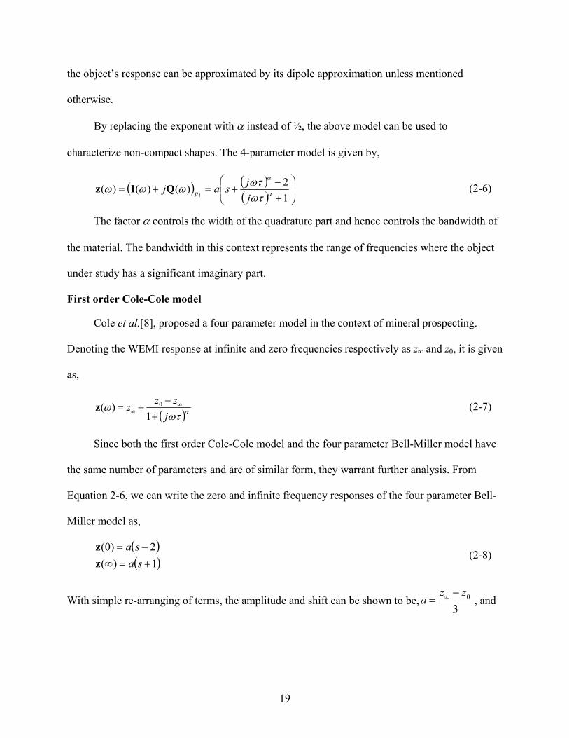
By replacing the exponent with α instead of ½, the above model can be used to
characterize non-compact shapes. The 4-parameter model is given by,
( ) ( )( ) ⎟⎟
⎠
⎞⎜⎜⎝
⎛
+−
+=+=12)()()(
4 α
α
ωτωτωωωjjsaj pQIz (2-6)
The factor α controls the width of the quadrature part and hence controls the bandwidth of
the material. The bandwidth in this context represents the range of frequencies where the object
under study has a significant imaginary part.
First order Cole-Cole model
Cole et al.[8], proposed a four parameter model in the context of mineral prospecting.
Denoting the WEMI response at infinite and zero frequencies respectively as z∞ and z0, it is given
as,
( )αωτω
jzzz
+−
+= ∞∞ 1
)( 0z (2-7)
Since both the first order Cole-Cole model and the four parameter Bell-Miller model have
the same number of parameters and are of similar form, they warrant further analysis. From
Equation 2-6, we can write the zero and infinite frequency responses of the four parameter Bell-
Miller model as,
( )( )1)(
2)0(+=∞−=
sasa
zz
(2-8)
With simple re-arranging of terms, the amplitude and shift can be shown to be,3
0zza
−= ∞ , and

20
0
02zzzz
s−+
=∞
∞ . Substituting the notations for a and s, the four-parameter model becomes,
( )Cole.Coleorderfirst
1)( 0 −≡
+−
+= ∞∞ αωτ
ωj
zzzz
Hence, the 4-parameter model proposed by Miller et al. defaults to 1st order Cole-Cole
model [8].
Figure 2-4. Effect of varying τ and α.
Figure 2-4 shows the effect of varying τ and α in the shape of the curve in the In-phase vs.
Quadrature-phase plot, also known as the Argand diagram. As τ goes outside a boundary of
values, only part of the shape is visible in the Argand diagram due to the finite bandwidth of
operation. Therefore the range of τ is limited by the bandwidth of the sensor.
In most unexploded ordnance (UXO) objects, there are soft metal rings near the tail of the
projectile, known as driving bands to facilitate being fired by a gun. This can be modeled by
extending the 4-parameter model into a 5-parameter model as,

21
( ) ( )( )
( )( ) ⎟
⎟⎠
⎞⎜⎜⎝
⎛
+
−+
+−
+=+=12
12)()()(
5 α
α
α
α
ωτωτ
ωτωτωωω
Loop
Loopp j
jb
jjsajQIz (2-9)
where τLoop = 101.295τ and cLoop = 0.943 are fixed empirically. This can be shown as a special case
of 2nd order Cole-Cole model.
While Bell-Miller models provide a framework for analyzing the electromagnetic
induction spectra, they don’t provide a fast way of estimating the parameters. There have been
many attempts at finding exact or approximate solutions to the first order Cole-Cole model, some
of which are described in the following sections.
Nonlinear least squares optimization
The most straightforward albeit computationally intensive method to estimate the
parameters is to use iterative least squares curve fitting approach. If ω1, ω2… ωNf are the
frequencies at which measurements are taken, then the parameters are given by,
( )( )∑
=⎟⎟⎠
⎞⎜⎜⎝
⎛
+−
+−=fN
k k
kk
csa jjsacsa
1
2
,,, 12)(minarg}ˆ,ˆ,ˆ,ˆ{ α
α
τ τωτωωτ z (2-10)
with the constraint that the parameters are real. This is usually achieved by using an iterative
least squares curve fitting algorithm. However, it requires a good initial estimate for converging
to the global or at least a good optimum. In practice, this requires the algorithm to be run
multiple times with different random initial conditions to find the optimal solution. The ways of
selecting the initial conditions and the number of epochs required are usually heuristic. It is also
a common practice to first divide the data by its total norm and then finally rescale the estimated
amplitude.
Bishay’s circle fitting method
Claim 2-1: If the spectral signature follows the Cole-Cole model, then the plot of I(ω) vs.
Q(ω) will be a segment of a circle.

22
Proof: Let us assume that the points from a first order Cole-Cole model indeed form a
segment of a circle. Let the center of the circle be at (ac,-bc), then the points from the model
intersect the x axis at (z0,0) and (z∞,0)
From Figure 2-5, the I(ω) coordinate of the center lies where Q(ω) reaches its maximum.
Taking the derivative Q(ω) of with respect to ω,
Figure 2-5. Real vs. imaginary parts of data from a first order Cole-Cole model.
At the maximum of Q(ω), the derivative is zero. Ignoring cases where ω = 0, ω = ∞ and
α = 0, the maximum happens at ω = 1/τ. Denoting the maximum by Qmax we get
.4
tan2
3)/1(max ⎟⎠⎞
⎜⎝⎛===
απτω aQ Q
The x coordinate of the center is given by ac = I(ω=1/τ) = a(s-1/2). From the figure, radius
is given by r = bc + Qmax. By using (I(ω)-ac)2 + (Q(ω)+bc)2 = r2 constraint, we get
(I(ω)-a(s-0.5))2+(Q(ω)+r-Qmax)2 = r2
Substituting for I(ω), Q(ω) and Qmax and solving for r, we get
( ) ( )( )
( ) ( ).
2cos21
2sin1
3)(2
2
2
⎟⎟⎟⎟⎟
⎠
⎞
⎜ ⎜ ⎜ ⎜ ⎜
⎝
⎛
⎟⎠
⎞⎜ ⎝ ⎛
⎟⎠⎞
⎜⎝⎛++
⎟⎠⎞
⎜⎝⎛+−
−=∂
∂ απωτωτ
απωτ
ωωτ α
ω ω
αα
ααa Q
I(ω)
(a, Qmax)
(ac,-bc) (z(∞),0) (z0, 0)
Q(ω)

23
⎟⎟⎠
⎞⎜⎜⎝
⎛⎟⎠⎞
⎜⎝⎛−⎟
⎠⎞
⎜⎝⎛=⎟
⎠⎞
⎜⎝⎛=
2tan
2cosec
23and
2cosec
23 απαπαπ abar c
Therefore, the first order Cole-Cole equation can be written as
( ) ( )222
2cosec
23
2tan
2cosec
23
21
⎟⎟⎠
⎞⎜⎜⎝
⎛⎟⎠⎞
⎜⎝⎛=⎟⎟
⎠
⎞⎜⎜⎝
⎛⎟⎟⎠
⎞⎜⎜⎝
⎛⎟⎠⎞
⎜⎝⎛−⎟
⎠⎞
⎜⎝⎛−+⎟⎟
⎠
⎞⎜⎜⎝
⎛⎟⎠⎞
⎜⎝⎛ −−
απαπαπωω aasa QI (2-11)
The cases where α > 1 correspond to the segment being greater than a semicircle and vice
versa. If Nf denotes the number of frequencies where measurements are made, then in cases
where z(0) and z(∞) can be measured, the values of τ and α can be estimated as [9] :
( )( ) ( )
( )( ) ( )∑
=
−−⎥⎦
⎤⎢⎣
⎡⎟⎟⎠
⎞⎜⎜⎝
⎛−∞
+⎟⎟⎠
⎞⎜⎜⎝
⎛−
=fN
k k
k
k
k
fN 1
11 tan0
tan21ω
ωω
ωπ
αIz
QzI
Q , and (2-12)
( ) ( )( ) ( )( ) ( )( ) ( )∑
=⎥⎦
⎤⎢⎣
⎡
+−∞+−
=fN
k kk
kk
kfN 1
21
22
22011 α
ωωωω
ωτ
QIzQzI
. (2-13)
Since in most practical applications, z(0) and z(∞) cannot be directly measured, they have
to be estimated. If the measured data includes the maximum of Q(ω) at frequency ωm, then
2I(ωm) ≈ z(0) + z(∞). Since z(0) and z(∞) are the I(ω)-axis intercepts, they are given by, z(0) =
ac - (r2-bc2)1/2 and z(∞) = ac + (r2-bc
2)1/2. The value of bc is positive if α > 1 and is negative if α <
1. The values of ac, bc and r are found by using least squares search with the constraint (I(ω) -
ac)2 + (Q(ω) - bc)2 = r2. This approach works well for spectral shapes that fall on a circle but is
not robust against noise and deviations from the assumed shape. Also, in cases where z(ω) has
flat regions, r ≈ ∞ which makes the estimate unstable.
Xiang’s direct inversion method
Pelton et al. [10] formulated the Cole-Cole model in terms of induced polarization (IP)
parameters in the form,
( ) ( )( ) ⎥
⎥⎦
⎤
⎢⎢⎣
⎡⎟⎟⎠
⎞⎜⎜⎝
⎛
+−−= αωτ
ωj
m1
1110zz , with ( )( )0
1zz ∞
−=m . (2-14)

24
The Xiang inversion method [11] converts the parameter estimation into a 1-D problem
using elimination of variable to estimate the parameters of the Pelton model, and hence is more
computationally efficient, but restricts the values of m and α to be between 0 and 1. This proves
to be a handicap in modeling certain low metal mines as shown in the experiments.
Bayesian inversion
Since direct inversion of the first Cole-Cole may lead to sub-optimal solutions, a Bayesian
approach [1] can be used to find the global optimum. z(0) and τ are characterized using Jeffreys
priors or alternately, log10(z(0)) and log10(τ) by uniform probability density. Also, by making a
change of variable from m to m’ using m’=log10(m/(1-m)), it can be represented by a uniform pdf.
And finally, by characterizing α by a uniform pdf, the Bayesian a posteriori probability
distribution is given by:
p(θ)=aτ z(0)m(1-m)π(θ)exp[-0.5*( z - zr(θ))TCdd-1(z - zr(θ))] (2-15)
where p(θ) represents the a priori probability density of the model parameters, zr(θ) the
reconstructed data and Cdd is the NxN data covariance matrix. The individual parameters are
found by finding the respective marginal pdfs. Though this method can produce accurate
estimates for the parameters with the right choice of priors, it is computationally intensive as the
posteriors do not have closed form solutions and hence need to be estimated by n-dimensional
grid search.
Discrete Spectrum of Relaxation Frequencies
The EMI response of a target can be modeled as a sum of real exponentials which, in
frequency domain can be represented as poles in the spectrum [12]. They are represented as:
( ) ∑= +
+=K
k k
k
jcc
10 1 ωτ
ωz , with τk ≥ 0 and ck ≥ 0. (2-16)

25
The values ck are estimated by searching for the ζk = 1/τk values in the region where
ωτk>10-2 to 102. Since ck are restricted to be real and positive, the matrix setup shown in
Equation 2-16 is solved using non-negative least-squares for real and imaginary components in
parallel.
c
KM
c
cc
MN MNjNjNj
Mjjj
Mjjj
Θ=
>>
⎥⎥⎥⎥⎥⎥⎥⎥
⎦
⎤
⎢⎢⎢⎢⎢⎢⎢⎢
⎣
⎡
⎥⎥⎥⎥⎥⎥⎥⎥
⎦
⎤
⎢⎢⎢⎢⎢⎢⎢⎢
⎣
⎡
=
⎥⎥⎥⎥⎥⎥⎥⎥
⎦
⎤
⎢⎢⎢⎢⎢⎢⎢⎢
⎣
⎡
+++
+++
+++
z
z
zz
.
.
.
...1...............
...1...1
)(...
)()(
1
0
2
1
/11
2/11
1/11
/211
2/211
1/211
/111
2/111
1/111
ζωζωζω
ζωζωζω
ζωζωζω
ω
ωω
. (2-17)
Figure 2-6. Effect of pole spread on DSRF coefficients. A) Argand diagram of the original and reconstructed signals. B) DSRF pole locations and their strengths. Since DSRF assumes the pole spread to be unity, it splits a single pole into many for low α values. In other words, DSRF tries to model the curve in the Argand diagram by a weighted sum of semi-circles.
-2 -1.5 -1 -0.5 0 0.5 1 1.5 2
x 10-4
0
0.5
1x 10
-4
ℜ(Z(ω))
ℑ(Z
( ω))
HMAP α=0.47 tau=1.1674e-005
103
104
105
106
0
0.5
1x 10
-4
ζ
c k
GRANMADSRFOriginalDSRF2DSRF3DSRF4DSRF5DSRF6
B)
A)

26
If the data is in fact generated from a Cole-Cole model with α<1, the DSRF splits a single
pole into multiple poles to make an accurate fit. In other words, DSRF tries to model the curve in
the Argand diagram which is a segment of a circle smaller than a semi-circle by a weighted sum
of semi-circles. This makes the characterization and classification of objects difficult.
Kth Order Cole-Cole
In the analysis of dielectric properties of biological tissues, the spectral shapes are more
complicated than that of the first order Cole-Cole model [13]. By generalizing the DSRF, we
may be able to model complicated shapes with lesser number of parameters. This leads to a
generalized version of the Cole-Cole equation as:
( )( )∑
= ++=
K
k k
kkj
cc1
0 1 αωτωz , with ck ≥ 0. (2-18)
This form of Kth order Cole-Cole model with K=4 is widely used in breast tumor detection
and other wideband EMI applications in medicine and biology. Direct inversion of a Kth order
Cole-Cole model is mathematically intractable. There however, exist a few methods that attempt
to find approximate solutions.
If the order K is known, then an iterative least squares method can be used to find the ck’s
and τk’s. The finite difference time domain method is also widely employed by the biological
tissue analysis community. Both these methods however require a good estimate of the initial
conditions and are computationally inefficient.

27
CHAPTER 3 TECHNICAL APPROACH
The focus of this research was on developing tools for detecting, analyzing and identifying
objects from sets of spectral measurements obtained from a wideband EMI sensor. Three specific
approaches, namely Prototype Angle Matching (PRAM), Gradient Angle Model Algorithm
(GRANMA) and Gradient Angle in Parts Algorithm (GRANPA), using the gradient angle
between the real and imaginary components of the data were developed each building on the
previous one and in the order of increasing complexity on simple spectral signatures. GRANMA
and GRANPA express the data in terms of their dielectric properties by extracting features
related to the underlying physical phenomena. PRAM and GRANMA identify objects based on
distance to one or more nearest prototypes. PRAM is a fast prototype matching method based on
gradient angles calculated numerically on the spectral signatures. GRANMA uses the gradient of
an analytical model, and reduces the number of parameters to be estimated simultaneously from
four to two. It significantly reduces the complexity of the search using a two stage approach.
GRANPA uses piecewise curve fitting to model more complicated spectra. It provides unique
solutions to model near field effects and is faster than existing methods.
A fourth method, SPARse DIelectric Relaxation estimation (SPARDIR), was introduced
that looks for a jointly sparse solution to provide the most compact representation of the data.
SPARDIR also separates the underlying physical phenomena from the sensor setup. Two
solutions to this algorithm, SPARDIR2 and SPARDIR1 were developed based on minimizing
quadratic and absolute error respectively. Although both methods provide sparse solutions and
approximate the data well, the first one is faster whereas the second one provides solutions closer
to the true underlying physics.

28
In the following section, we briefly review the Argand diagram and explain the four
methods, PRAM, GRANMA, GRANPA and SPARDIR.
Argand Diagrams of WEMI Responses
Argand diagrams have been one of the widely used tools to study complex data. They are
also known as Nyquist plots in the context of control theory and Cole-Cole plots in
electrochemistry. It is a plot of In-phase component I(ω) against the Quadrature-phase
component Q(ω). Figure 3-1 shows that it provides a consistent framework to identify specific
mine types. Mines with similar metal content have similar signatures (which may not be true in
the case of Ground Penetrating Radar). This property can be exploited in landmine detection and
classification.
Figure 3-1 Argand plots of WEMI response for a A) boxed AP mine and a B) circular AT mine at different locations and depths. Different points in the curve represent the WEMI response at different frequencies.
Figure 3-1 shows that though the shapes are similar, there is variability in the amplitude
and in the shift in In-phase component between different candidates of same mine type. The
B)
A)

29
slope between the points in the Argand diagram is a powerful tool for discrimination. Figure 3-2
shows that, the variability between different candidates is reduced as the gradient angle is
independent of amplitude and shift, two of the most difficult and unreliable (Fails, et al., 2007)
values to estimate. Here the angles are calculated numerically by using a two-sided gradient.
)()()()()()(
ωωωωωωωωωω
Δ−−Δ+=∂Δ−−Δ+=∂
IIIQQQ
.
The gradient angle is defined as
( ))(),()( ωωω IQm ∂∂= atan2 (3-1)
Using the MATLAB® definition of atan2, the equation for the gradient angle is given by:
⎟⎟
⎠
⎞
⎜⎜
⎝
⎛
∂+∂+∂
∂= −
22
1
))(())(()()(tan2)(
ωωωωω
QIIQm . (3-2)
Prototype Angle Matching
The Prototype Angle Matching method is a nearest prototype classifier. The prototype of
each object class is defined to be point-wise median. More precisely, if Ti represents the set of
indices of all candidates of object type i, then the corresponding set of gradient angles is given by
Mi(ω)={mk(ω) : for all k ∈ Ti} and the prototype by:
( ) ( )[ ]ωω kk
i mmedianP = (3-3)
If z is a test vector, then the confidence that z is of target class is defined by
))((11)( δγ −−+
= zztde
conf (3-4)
where ),(min)( iit Pdd zz = is defined to be the distance between z and the target class t and γ
and δ are the rate and bias parameters of the logistic function to be estimated by cross validation
[15].

30
Figure 3-2. Angle plots of WEMI response for a A) circular AT mine and B) boxed AP mine and
at different locations and depths.
Gradient Angle Model Algorithm
Parameters of the Cole-Cole model have been used successfully [14] to model and classify
metallic objects. The most widely used parameter estimation methods use nonlinear optimization
methods, which are slow due to the presence of local minima. The simpler methods are faster but
not robust against noise and deviations from the model. In this section, it is shown that by
analytically differentiating the Cole-Cole model, a fast lookup algorithm can be formulated. This
is one of the contributions of the present research.
Separating the I(ω) and Q(ω) components using MATHEMATICA®, (verified numerically
and by MATLAB® symbolic math toolbox) the four-parameter model becomes:
B)
A)

31
( )
( ) ( ) ⎟⎟⎟⎟⎟
⎠
⎞
⎜⎜⎜⎜⎜
⎝
⎛
⎟⎠⎞
⎜⎝⎛++
⎟⎠
⎞⎜⎝
⎛⎟⎠⎞
⎜⎝⎛+
−+=
2cos21
2cos13
1)(2 απωτωτ
απωτω
αα
α
saI , and (3-5)
( )
( ) ( ).
2cos21
2sin3
)(2
⎟⎟⎟⎟
⎠
⎞
⎜⎜⎜⎜
⎝
⎛
⎟⎠⎞
⎜⎝⎛++
⎟⎠⎞
⎜⎝⎛
=απωτωτ
απωτω
αα
α
aQ (3-6)
Using the same framework as Equation 3-2, the equation for the gradient angle for four-
parameter model (assuming a > 0) is
( )( ) ⎟⎟
⎠
⎞⎜⎜⎝
⎛⎟⎠⎞
⎜⎝⎛
++−
= −
4tan
11tan2)( 1 απ
ωτωτω α
α
m (3-7)
The range of m(ω) is given by evaluating it at the extrema of ωτ :
2)(and
2)(
0
απωαπωωτωτ
−==∞==
mm .
These equations show that the angle varies between απ/2 and – α π/2 which is adequate to
model all angles when α ∈ [0, 2]. They also show that the three-parameter Bell-Miller model
(Miller, et al., 2001), where α is restricted to be equal to 0.5, can only characterize angles
between -π/4 and π/4. Analysis of empirical data shows the latter range to be inadequate.
Since the equation for the gradient angle involves only two variables, a lookup table was
created for m(ω) for a range of values of τ and α. The elements of the table are denoted by
( )ταω ,,m̂ . Values of τ and α were found by calculating the best match between m(ω) and table
values using least mean absolute error:
∑ −=ω
ταωωτα ),,(ˆ)(),(ˆ mmE (3-8)
The lookup table error EL is defined as follows:

32
⎟⎟⎠
⎞⎜⎜⎝
⎛== ),(ˆ,minargˆ,ˆwhere)ˆ,ˆ(ˆ τατα
τατα EELE (3-9)
The amplitude a was found by substituting the estimates τ and α in Equation 3-6 and
finding the maximum likelihood estimate:
( )( )( ) ⎥
⎦
⎤⎢⎣
⎡
+−
=
1ˆ2ˆ
Imˆ
ˆ
ˆ
α
α
τωτωω
jj
a Q (3-10)
where τ̂ and α̂ are lookup table estimates, and Nf is the number of measured frequencies
Finally, the shift s was found by substituting the estimates of a, τ and α in Equation 3-5:
( ) ( )( ) ⎥
⎦
⎤⎢⎣
⎡
+−
−=1ˆ2ˆ
Reˆ
ˆ ˆ
ˆ
α
α
τωτωω
jj
as I (3-11)
The goodness of fit for this method was measured as the normalized error between the
actual data and the fit:
( )( )
.)(
1ˆ2ˆˆˆ)(
1
2
1
2
ˆ
ˆ
∑
∑
=
=⎟⎟⎠
⎞⎜⎜⎝
⎛
+−
+−
=f
f
N
kk
N
k k
kk
F
jjsa
Eω
τωτωω α
α
z
z (3-12)
Stability of Lookup Table Step in GRANMA
All the parameter estimates depend on the accuracy of the gradient and on the resolution of
the table. Therefore, first it was necessary to see how a small error in the parameter estimate in
the (τ, α) space due to the finite size of the lookup table affects the angle estimate. Figure 3-3
shows the dependence of m on τ and α for a fixed ω. It shows two regions of interest, one being
α = 0, and another α = 2. Figure 3-4 shows that near regions where ωτ = 1, there is a large
change in m for small changes in τ and α due to the fact that the denominator in Cole-Cole
equation becomes zero. Therefore, regions too close to α = 2 were avoided.

33
Figure 3-3. Plot of gradient angle m in degrees vs. ωτ and α. It shows a discontinuity in m when
α = 2 and ωτ = 1.
Figure 3-4. A) ∂m/∂τ and B) ∂m/∂α of the proposed model, computed numerically, shown at
330Hz. It shows the pattern that, near to regions where ωτ ≈ 1 and α ≈ 2, there is a big difference in the angles for a small change in τ or α.
10-1
100
101
0
0.5
1
1.5
2
-100
0
100
α
Gradient angle in parameter space for a fixed ω
ωτ
m( ω
, τ, α
)
α α
A)
B)

34
Next, it was necessary to analyze the robustness of the estimated parameters with respect
to noise in the data and in the gradient estimates. Since the noise in the parameters is non-linearly
linked to the noise in the data, it is difficult to derive expressions linking the noise in them.
Therefore, the stability of the method with respect to noise in the data was analyzed in the
context of classifier design.
Classifier Design
The classification was done on six features using a soft K nearest neighbor method. The
features are a, tan-1(s), log10(τ), α, EL & EF defined in Equations 3-9 to 3-12. The value of K was
found as the one that gave minimum variance without sacrificing performance. The confidence
value for object i is given by
∑
∑
=
== K
j
ij
K
j
ij
m
niconf
1
1)( (3-13)
where nij is the distance to jth nearest non-mine neighbor, and mi
j is the distance to jth mine
neighbor. The contribution here is the estimation of the Cole-Cole parameters, not in the
classifier design. Any suitable classifier could be used here.
Gradient Angles in Parts Algorithm
The first order Cole-Cole model together with GRANMA is useful for modeling objects
that show a single relaxation in their spectral signatures. This, however, may not be enough to
model objects that have more complicated spectral shapes. The Kth order Cole-Cole has found
many applications especially in electromagnetic studies in biology [13]. However, there are no
direct inversion methods available to estimate the parameters and existing methods are too slow
to be used in a real-time environment like landmine detection [13].
35
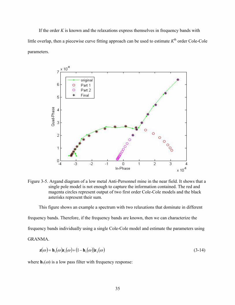
If the order K is known and the relaxations express themselves in frequency bands with
little overlap, then a piecewise curve fitting approach can be used to estimate Kth order Cole-Cole
parameters.
Figure 3-5. Argand diagram of a low metal Anti-Personnel mine in the near field. It shows that a single pole model is not enough to capture the information contained. The red and magenta circles represent output of two first order Cole-Cole models and the black asterisks represent their sum.
This figure shows an example a spectrum with two relaxations that dominate in different
frequency bands. Therefore, if the frequency bands are known, then we can characterize the
frequency bands individually using a single Cole-Cole model and estimate the parameters using
GRANMA.
( ) ( ) ( ) ( )( ) ( )ωωωωω 2111 1 zhzhz −+= (3-14)
where h1(ω) is a low pass filter with frequency response:

36
( )⎩⎨⎧
≥∈
=0
01 ,0
),0[,1ωω
ωωωh , with ω0 as the cutoff frequency.
This approach can be extended to a general Kth order case as a bank of band-pass filters:
( ) ( ) ( )∑=
=K
kkk
1
ωωω zhz , with ( )∑=
=K
kk
1
1ωh for all ω. (3-15)
Now, the problem of estimating Kth order Cole-Cole equations simplifies into finding the
band-pass filters, so that individual bands can be modeled using a first order Cole-Cole model.
Filter Design
Figure 3-6. A) Argand diagram of a low metal Anti-Personnel mine in the near field. B)
gradient angle at different frequencies. C) slope of gradient angle
A)
B)
C)

37
There are many ways of finding the optimal cutoff frequency in two filter case. One of the
easiest is to search exhaustively in the frequencies of interest (usually around the middle
frequency) to optimize for the least lookup table error. Another method would be to find the
location of the gradient angle minimum around the center frequency as shown in Figure 3-6 B.
Another option would be to choose the frequency where slope of gradient angle crosses from
negative to positive around the center frequency as shown in Figure 3-6 C. We found the zero
crossing to be a reliable estimate of the cutoff frequency for landmine data. Experimental results
demonstrated that a less heuristic method should be pursued. There is one merit that should be
mentioned here. GRANPA provides a simple and fast way of estimating the near field effects.
Classifier Design
A soft kNN classifier similar to the one used in GRANMA case could be used. Relevance
Vector Machines (RVM) also show promise in case of GRANMA features and could be used
here. This method is applicable only when the order K is known and the relaxations are
bandwidth limited.
Dielectric Relaxation estimation using Sparse Models
We can use similar to the framework used by DSRF to model such curves. By extending
the matrix T to include different values of τ and α, we get:
( ) ( ) ( ) ( ) ( ) ( ) ( )
( ) ( ) ( ) ( ) ( ) ( ) ( )
( ) ( ) ( ) ( ) ( ) ( ) ( ) ⎥⎥⎥⎥⎥⎥⎥⎥
⎦
⎤
⎢⎢⎢⎢⎢⎢⎢⎢
⎣
⎡
⎥⎥⎥⎥⎥⎥⎥⎥
⎦
⎤
⎢⎢⎢⎢⎢⎢⎢⎢
⎣
⎡
=
⎥⎥⎥⎥⎥⎥⎥⎥
⎦
⎤
⎢⎢⎢⎢⎢⎢⎢⎢
⎣
⎡
+++++++
+++++++
+++++++
MLN c
cc
LcMNjLc
NjcNjc
NjLcNjc
NjcNj
LcMjLcjcjcjLcjcjcj
LcMjLcjcjcjLcjcjcj
.
.
.
.........1...
.........1
.........1
)(...
)()(
1
0
2
1
1
1
21
1221
1121
1
11
1211
1111
1
21
1
221
12221
11221
1
121
12121
11121
1
11
1
211
12211
11211
1
111
12111
11111
1
τωτωτωτωτωτωτω
τωτωτωτωτωτωτω
τωτωτωτωτωτωτω
ω
ωω
z
zz

38
or,
( )( ) ]/[,mod11,
1
1, LjIntegermLjn
ncmij
ji =−+==
=
⎟⎠⎞
⎜⎝⎛+ τω
θ
Θcz (3-16)
The values of ck can be found using many different approaches, some of which are
described in the following section. Since the ck’s are restricted to be real whereas, Θ and z are
complex, the optimization is done as
( )( )
( )( ) cΘΘ
zz
⎥⎦
⎤⎢⎣
⎡ℑℜ
=⎥⎦
⎤⎢⎣
⎡ℑℜ
me
me
. (3-17)
Non-negative Least Squares Optimization
This uses the same approach as in DSRF. This approach has the advantage of being able to
estimate ck’s and the order K simultaneously. However, this almost always over-estimates K, and
needs to be modified with a sparsity constraint on the ck’s as described in the next method.
Convex Optimization with Sparsity Constraint
Both DSRF and SPARDIR can be written in matrix form as Θcz = with Θ being the
dictionary of dielectric relaxations of interest. Each column in Θ corresponds to a realization of a
first order Cole-Cole or Debye model normalized to have a unit L2 norm. In general, the
dimension of z is lesser than the number of columns in Θ. Also the columns themselves are
correlated. This leads to an over-complete problem with multiple solutions. However, if we
assume that only a few ck’s are nonzero, then we are essentially looking for the smallest order
Cole-Cole or Debye model to fit our data. This transforms the problem of estimating the
dielectric relaxations into a constrained optimization problem given as
(P0) Minimize 0c subject to Θcz = (3-18)

39
with 0c being the L0 norm which is the number of nonzero elements in c. Even though L0 norm
does not satisfy the requirements for a norm, it is still referred to as a norm.
The constrained optimization problem as given in Equation 3-18 is NP hard [16]. There is
no direct method of optimizing with the L0 norm constraint. However there are three alternate
approaches to solving such problems. These approaches are desirable because they can converge
to the original solution for problem P0 under certain conditions. If we let u be the parameter
controlling the trade-off between fitting error and the sparsity of the final solution, then
• (P1) L1 constrained optimization: minimize ( )∑=
−+−L
kkcuu
1
2
21Θcz . (3-19)
• (P2) Lp constrained optimization:
minimize ( )∑=
−+−L
k
pkcuu
1
2
21Θcz , with 0<p< 1 (3-20)
• (P3) Iterative reweighted optimization:
minimize ( )∑=
−+
+=−+−
L
kp
k
nkkk
ccuu
11
)1(2
2
1,1ε
γγΘcz , (3-21)
with 0 < p < 1, and ε ≈ 0.
There are multiple ways of solving the above mentioned three optimization problems.
Some of the famous ones are quadratic programming, linear programming, projected gradient
and gradient descent.
The uniqueness of the solutions to problems P1-P3 depends on the correlation between the
columns of Θ. If jT
ijiLjiθθ
≠∈=
];,1[,maxμ denotes the maximum correlation between any two columns
in the dictionary, then if the number of nonzero coefficients or model order K for the true L0
solution satisfies

40
K = 0c < 0.5 (1+1/μ) (3-22)
[16] then the L1 norm based solution of P1 is the same as the L0 norm based solution in Equation
3-18 [16]. The Lp norm based solution of P2 can equal to the L0 norm based solution of P0 under
more relaxed conditions. In general, the conditions depend on the Restricted Isometry Property
(RIP) of the matrix Θ [18]. It states that to produce K-sparse solutions, the matrix Θ has to
satisfy
( ) ( ) KLKK ≤ℜ∈∀+≤≤−
0
2
2
2
2
2
2,11 zzzΘzz δδ (3-23)
with δK < 1. For L1 norm solution to reach the L0 norm solution, the condition is δK < 2 - 1. For
an Lp norm solution to give a unique L0 solution, the condition is
( ) 211
111221
11−
⎟⎠⎞
⎜⎝⎛ +−+
−<p
K
K
δ [18]. When p is close to zero, δK is close to 1. So the interval [1-
δK, 1+δK] is larger, yielding more relaxed conditions. This makes Lp optimization to give better
solutions than with p = 1. In other words, as p decreases, the condition for reaching the L0
solution becomes easier to satisfy. However, when p < 1, the problem is no longer convex and
hence achieving a global optimum depends on the algorithm and its initial conditions.
Quadratic programming
The optimization problems shown in Equation 3-19 and Equation 3-21 can be solved by
quadratic programming which tries to minimize the function 0.5xTAx+bTx with respect to x for x
≥ 0. For a simple x ≥ 0 constrained optimization, A= ΘΤΘ and b=-zTΘ. When we add the L1
constraint, the inputs become A= ΘΤΘ and b = -zTΘ +1, where 1 is a vector of ones of
appropriate length. For iterative reweighted optimization with a given p, the input A remains the
same while b = -zTΘ +γ, with γ being a vector containing the γk’s. We used MATLAB®’s

41
quadprog.m function to implement this method. This iterative schedule is summarized in the
following pseudo-code
Q_IR
1. A← ΘΤΘ 2. γk ← 1 for all k 3. Scale z for unit norm and positive sign 4. b ← -zTΘ +γ 5. Iteration ← 1 6. while |ObjectiveFunctionValue- PreviousObjectiveFunctionValue| > ChangeThreshold
a. PreviousObjectiveFunctionValue ← ObjectiveFunctionValue b. Compute c to minimize 0.5cTAc+bTc c. Update γk =1/|ck| d. if γk > SparsityParameterThreshold then
i. Remove kth column of Θ ii. Remove γk from γ
iii. Update A← ΘΤΘ end if
e. Update b ← -zTΘ +γ f. Update ObjectiveFunctionValue ← 0.5cTAc+bTc g. Iteration ← Iteration + 1
7. end while 8. Re-scale c with original scale and sign of z.
Linear programming
The linear programming approaches focus on minimizing functions of the form fTx subject
to Θcz = . For L1 constrained optimization, f is a vector of ones. For iterative reweighted
optimization f = γ, with γk’s being updated iteratively. This makes the approach a sequence of
linear programming solutions all with the same region of feasibility. We used MATLAB®’s
linprog.m function to implement this method. This iterative schedule is summarized in the
following pseudo-code
L_IR
1. γk ← 1 for all k 2. Scale z for unit norm and positive sign 3. f ← γ 4. Iteration ← 1

42
5. while |ObjectiveFunctionValue- PreviousObjectiveFunctionValue| > ChangeThreshold a. PreviousObjectiveFunctionValue ← ObjectiveFunctionValue b. Compute c to minimize fTc c. Update γk =1/|ck| d. if γk > SparsityParameterThreshold then
i. Remove kth column of Θ end if
e. Update f ← γ f. Update ObjectiveFunctionValue ← fTc g. Iteration ← Iteration + 1
6. end while 7. Re-scale c with the original scale and sign of z.
There are two common ways to implement linear programming namely, the simplex
method and the interior point method. The explanation of those methods is beyond the scope of
this thesis.
Joint Sparse Estimation of Dielectric Relaxations
All the methods mentioned so far use a single observation to identify objects. In practical
use, most often multiple measurements are taken around an object with varying orientations and
distances. If we can assume the observed data is a weighted sum of parts with each part due to a
different component, then multiple measurements around an object should contain the same set
of parts albeit with different set of weights. For example if θ1 and θ2 are responses due to two
sources, then observations are given by z1=w1θ1+w2θ2 and z2= w3θ1+w4θ2, with w1 to w4 being
the appropriate weights. Therefore it is preferable to use all the responses related to an object
together to get a more stable estimate.
The optimization now becomes a joint sparse estimation with the group of observations
coming from the same small subset of the dictionary. If H denotes the Heaviside step function,
then the optimization function for No observations is given by,

43
(JP0) Minimize ∑= ∈
⎟⎠⎞⎜
⎝⎛=
L
kjkNj
cHKO1
,],1[max subject to
( ) ( ) ( )[ ] ( ) ( ) ( )[ ] ΘCcccΘzzzZ === ONO ...... 2121 . (3-24)
Joint sparsity implies that the matrix C is row sparse i.e. only a few rows have nonzero
elements. The problem given in Equation 3-22 is NP hard, therefore approximations similar to
Equations 3-18 to 3-20 can be extended in the joint case as
• (JP1) Lp,q constrained optimization: minimize ( )∑ ∑= =
⎟⎟⎠
⎞⎜⎜⎝
⎛−+−
L
k
pN
j
q
jk
O
cuu1 1
,2
21ΘCZ , (3-25)
with 0 < p < 1 and q > 1.
• (JP2) Iterative reweighted optimization:
minimize ( )∑∑
∑=
−
=
+
=+⎟⎟
⎠
⎞⎜⎜⎝
⎛=⎟⎟
⎠
⎞⎜⎜⎝
⎛−+−
L
kp
O
jjk
nk
N
j
q
jkk
c
cuuO
11
1,
)1(
1,
2
2
1,1
ε
γγΘCZ , (3-26)
with 0 < p < 1, q ≥ 1 and ε ≈ 0.
• (JP3) L1 optimization: minimize ( )∑∑= =
−+−L
k
N
jjk
O
cuu1 1
,11ΘCZ . (3-27)
The advantage of such joint sparse optimization as opposed to optimizing each observation
individually is that we can uniquely estimate a K sparse solution with K < 0.5(1/μ + Rank(Z) ) as
opposed to 0.5(1+1/μ) [17]. This enables us to estimate higher order models for a given
dictionary, or design dictionaries with more elements which in turn produce more accurate
answers.
As in the single observation case, the quadratic programming or linear programming
approaches can be used to solve Equation 3-24. The A matrix remains the same, while b(j) =
z(j)TΘ +γT. The entries in the γ vector now correspond to the sums along the rows of C rather than

44
the individual elements in each of the columns. This definition of γ enforces joint sparsity by
using the same sparsity parameter γk along all columns of a given row of C.
Gradient Newton Methods
The quadratic and linear programming methods work well when all the weights are non-
negative. However, this may not be the case with all WEMI data. For example, in landmine
detection using a Dipole transmitter antenna and a Quadrupole receiver antenna, each of the
relaxations can have positive or negative weights. In case of multiple observations the magnitude
and sign of the weights vary with respect to the relative distance and orientation between the
object and the antenna setup. In such cases, a gradient descent approach can be used to solve
Equations 3-24 to 3-26.
For the objective functions defined in Equations 3-24 to 3-26 of the form uE + (1-u)R,
Newton methods are given by the update equation for time step t+1 as ttt CCC Δ−=+ η1 , where η
denotes the step size tCΔ is the update which is given by
( ) ( ) ( ) ⎟⎟⎠
⎞⎜⎜⎝
⎛∂∂
−+∂∂
⎟⎟⎠
⎞⎜⎜⎝
⎛∂∂
−+∂∂
=Δ−
vvvvC
ttttt RuEuRuEuvec 11
1
2
2
2
2
, with E denoting the quadratic or linear
fitting error term, R the regularization term and v the vectorized version of C. vec( ) denotes the
vectorization operator.
Lp,q Regularized Optimization
To solve Equation 3-24, let us denote the quadratic fitting error and the regularization
terms as ( )∑∑ ∑== =
=⎟⎟
⎠
⎞
⎜⎜
⎝
⎛
⎭⎬⎫
⎩⎨⎧
=−=L
k
pk
pL
k
N
j
q
kj RcREO
11 1
2
2&ZΘC .
Taking partial derivatives, and using o to denote element-wise multiplication,

45
[ ]1...1...
2
)(2
1
11
⎥⎥⎥⎥⎥⎥
⎦
⎤
⎢⎢⎢⎢⎢⎢
⎣
⎡
=∂∂
=
−−=∂∂
−
−
pL
p
T
R
R
pR
qFor
E
CC
ZΘCΘC
To derive the Hessian matrix, first we need to vectorize the weight matrix.
⎥⎥⎥⎥⎥⎥⎥
⎦
⎤
⎢⎢⎢⎢⎢⎢⎢
⎣
⎡
=∂∂
=
.
....000...000...000
)(
2
2
ΘΘΘΘ
ΘΘ
v
Cv
T
T
T
E
vecLet
(3-28)
If LmmLkk mod&mod 11 == , with L being the number of columns of Θ, vk = ci1,j1, k =
(i1-1)L + j1 and m = (i2-1)L + j2, then the Hessian for the regularization term is given by,
⎪⎪⎩
⎪⎪⎨
⎧
=−
=+−
=∂∂
∂ −
−−
otherwise
mkifvvRpp
mkifpRvRpp
vvR
mkp
k
pkk
pk
mk ,0
,)1(4
,2)1(4
112
122
2
1
11
(3-29)
The Hessian matrix of the gradient descent controls the speed of convergence along each
of the weights. The matrix needs to be positive definite for the solution to converge. The problem
in using a Newton approach directly on Lp,q regularized optimization is that the second order
gradient matrix has p(p-1) term in the diagonal. Since p < 1, this may lead to negative diagonal
entries which can result in the solution to diverge.

46
Iterative Reweighted Optimization
We can extend the same treatment to JP2 as we did for JP1.
⎥⎥⎥⎥⎥⎥⎥⎥
⎦
⎤
⎢⎢⎢⎢⎢⎢⎢⎢
⎣
⎡
=
Lγ
γγ
...000...
0...000...00
Let
2
1
G
(3-30)
For q = 2, using a similar approach as in Lp,q optimization, the equations simplify to
( ) ZΘGΘΘC TT uuu 1)1( −−+=
(3-31)
This setup provides us with a simple equation that improves the solution by iteratively
updating G and C. This iterative schedule is summarized in the following pseudo-code
L2_IR
1. γk ← 1 for all k 2. Scale all columns of Z for positive sign 3. Compute G according to Equation 3-30 4. Compute C according to Equation 3-31 5. Iteration ← 1 6. while |ObjectiveFunctionValue- PreviousObjectiveFunctionValue| > ChangeThreshold
a. PreviousObjectiveFunctionValue ← ObjectiveFunctionValue
b. Update
∑=
←ON
jjk
k
c1
2,
1γ
c. if γk > SparsityParameterThreshold then i. Remove kth column of Θ
ii. Remove γk from γ iii. Update G according to Equation 3-30 iv. Update C according to Equation 3-31
end if d. Update ObjectiveFunctionValue according to Equation 3-26 e. Iteration ← Iteration + 1
7. end while 8. Re-scale C with original sign of Z.

47
L1 Optimization
To solve Equation 3-26, let ∑ ∑= =
⎟⎟⎠
⎞⎜⎜⎝
⎛
⎭⎬⎫
⎩⎨⎧
=−=L
k
N
jjkk
O
cRE1 1
,1||& γZΘC . Directly applying
second derivative approach is not possible as the derivative of L1 norm is the sign or signum
function which is discontinuous at 0 and has derivative equal to 0 elsewhere. However, the
hyperbolic tangent function can be used as a smooth approximation to the signum function with
a scaling constant β. As β increases, the approximation becomes better. Using the approximation
and taking partial derivatives, we obtain
( )( )ZΘCΘZΘCΘC
−≈−=∂∂ βtanh2)(2 TT signE
(3-32)
& ( ) [ ] ( ) [ ]1...1
.
.
.tanh21...1
.
.
.2
11
⎥⎥⎥⎥⎥⎥
⎦
⎤
⎢⎢⎢⎢⎢⎢
⎣
⎡
≈
⎥⎥⎥⎥⎥⎥
⎦
⎤
⎢⎢⎢⎢⎢⎢
⎣
⎡
=∂∂
LL
signR
γ
γ
β
γ
γ
CCC
(3-33)
Using ↓ to denote entries along a column, the update equation can be written as
( ) ( ) ⎟⎟⎠
⎞⎜⎜⎝
⎛
∂
∂−+
∂
∂−+=Δ ↓↓−
↓ CCHHC jjR
jEjj
Ru
Euuu 1)1( 1 , (3-34)
with jRj G.RH = , where G is the diagonal matrix with γk’s as its entries as defined in the previous
method and “.” denotes the matrix product.
Let
⎥⎥⎥⎥⎥⎥⎥⎥
⎦
⎤
⎢⎢⎢⎢⎢⎢⎢⎢
⎣
⎡
=
)(hsec...000...
0...0)(hsec0
0...00)(sech
,2
,22
,12
jL
j
j
j
c
c
c
β
β
β
βR . (3-35)

48
Using ( ) j↓−= ZΘCje to denote the jth column of the fitting error matrix, we can write the
Hessian matrix for the L1 fitting error as
ΘΘ
⎥⎥⎥⎥⎥⎥⎥⎥
⎦
⎤
⎢⎢⎢⎢⎢⎢⎢⎢
⎣
⎡
=
)(sech...000...
0...0)(sech0
0...00)(sech
,2
,22
,12
jL
j
j
TEj
e
e
e
H
β
β
β
β
(3-36)
This approximation has the property that it bridges the gap between L1 and L2 methods.
When β is near one, the approximation is close to the L2 method because tanh(x) ≈ x for small
values of x. As β increases the results become closer and closer to the L1 approach. This iterative
schedule is summarized in the following pseudo-code
L1_IR
1. γk ← 1 for all k 2. β ← 1 3. Scale all columns of Z for positive sign 4. Compute G according to Equation 3-30 5. Compute C according to Equation 3-31 6. Iteration ← 1 7. while |ObjectiveFunctionValue- PreviousObjectiveFunctionValue| > ChangeThreshold
a. PreviousObjectiveFunctionValue ← ObjectiveFunctionValue b. Compute ∂E/∂C according to Equation 3-32 c. Compute ∂R/∂C according to Equation 3-33 d. Compute Rj according to Equation 3-35 e. Compute Hessian of regularization term j
Rj G.RH ←
f. Compute Hessian of absolute error term according to Equation 3-36 g. Update C according to Equation 3-34
h. Update
∑=
←ON
jjk
k
c1
,
1γ
i. if γk > SparsityParameterThreshold then i. Remove kth column of Θ
ii. Remove γk from γ iii. Update G according to Equation 3-30

49
iv. Update C according to Equation 3-34 end if
j. Update ObjectiveFunctionValue according to Equation 3-27 k. Iteration ← Iteration + 1
8. end while 9. Re-scale C with original sign of Z.
Dictionary Learning using Adaptive Kernels
The set of methods discussed so far use a fixed dictionary. In most parametric modeling
approaches, the dictionary is populated using a specific model whose parameters are varied to
create dictionary elements. In the present case the model is a first order Cole-Cole model. The
task of creating a dense enough dictionary to represent data of interest while keeping the
correlation between the elements small is not trivial. For example, the Cole-Cole dictionary for
the frequencies between 300 Hz to 90000 Hz equispaced in log scale can have only a maximum
of 11 elements for a correlation threshold of 0.9. This is highly restrictive and still the correlation
is too high. One solution to alleviate this problem would be to make the dictionary tuned to the
data. ( )( ) k
kk αωτ
ωi1
1Let +
=θ denote kth dielectric relaxation. By extending the same gradient
descent approach to the regularized error function defined in Equation 3-26, we get for L2 error,
0&)(log
2log
=∂∂
−⎟⎟⎠
⎞⎜⎜⎝
⎛∂
∂=
∂∂
k
T
k
k
k
REτττ
ZΘCθ (3-37)
with ( ) ( )( )( )2i1
ilog k
k
kk
k
kαωτ
ωτατω
+−=
∂∂θ
(3-38)
0&)(2 =∂∂
−⎟⎟⎠
⎞⎜⎜⎝
⎛∂∂
=∂∂
k
T
k
k
k
REααα
ZΘCθ (3-39)
with ( ) ( ) ( )( )( )2i1
ilogik
k
k
kk
k
kα
α
ωτ
ωτωτα
ω
+−=
∂∂θ (3-40)

50
Note that since τ varies in exponential scale, the update is done using loge(τ ). The
Hessians are given by
( )( ) ( )( )
( )( )
( )( ) ( )( ) ( )( )
( )( )⎪⎩
⎪⎨
⎧=
+
+−=
∂∂∂
⎪⎩
⎪⎨
⎧=
+
+−=
∂∂∂
otherwise , 0
,i1
ilogi1i
otherwise , 0
,i1
i1i
loglog
3
22
3
22
mk
mk
k
kk
k
kk
k
kkk
mk
k
k
kkk
mk
k
α
αα
α
αα
ωτ
ωτωτωτ
ααω
ωτ
ωτωτα
ττω
θ
θ
Since the diagonal elements of the Hessian cannot be guaranteed to be positive, only a first
order update is used. Also, since the parameters are restricted to be real, only the real part of the
update is used. Using the same approach as Equations 3-37 to 3-40, the update equations for L1
error are given by
( )( ) 0&tanhlog
2log
=∂∂
−⎟⎟⎠
⎞⎜⎜⎝
⎛∂
∂=
∂∂
k
T
k
k
k
REτ
βττ
ZΘCθ (3-41)
and ( )( ) 0&tanh2 =∂∂
−⎟⎟⎠
⎞⎜⎜⎝
⎛∂∂
=∂∂
k
T
k
k
k
REα
βαα
ZΘCθ (3-42)
The dictionary elements are adapted along with their corresponding weights as described
below
AKL1_IR
1. γk ← 1 for all k 2. β ← 1 3. Scale all columns of Z for positive sign 4. Compute G according to Equation 3-30 5. Compute C according to Equation 3-31 6. Iteration ← 1 7. while |ObjectiveFunctionValue- PreviousObjectiveFunctionValue| > ChangeThreshold
a. β ← 1.005β b. PreviousObjectiveFunctionValue ← ObjectiveFunctionValue c. Compute ∂E/∂C according to Equation 3-32 d. Compute ∂R/∂C according to Equation 3-33

51
e. Compute Rj according to Equation 3-35 f. Compute Hessian of regularization term j
Rj G.RH ←
g. Compute Hessian of absolute error term according to Equation 3-36 h. Update C according to Equation 3-34
i. Update
∑=
←ON
jjk
k
c1
,
1γ
j. if γk > SparsityParameterThreshold then i. Remove kth column of Θ
ii. Remove γk from γ iii. Update G according to Equation 3-30 iv. Update C according to Equation 3-34 v. β ← 1
end if k. Update τk according to Equation 3-41 l. Update αk according to Equation 3-42 m. Update ObjectiveFunctionValue according to Equation 3-27 n. Iteration ← Iteration + 1
8. end while 9. Re-scale C with original sign of Z.
Double Dictionary Search
In most practical cases the joint sparse estimation is done over observations that are
generated by collecting data by varying the distance and orientation of the sensor setup with
respect to the object. The observations are then related to one another by the response function of
the transmitter and the receiver.
For example, Figure 3-7 shows the weights of individual relaxations for a high metal anti-
tank mine along a path known as down-track. We can see that the weights themselves follow a
pattern that is dependent on the dipole transmitter and quadrupole receiver configuration. We can
create another dictionary of such shapes and constrain the weights to a linear combination of
them as C = (HW)T, with H being the dictionary of down-track shapes. The matrix W now
serves as row sparse weight matrix for the dielectric relaxations and picks the down-track shapes
by the column values along such rows. By designing an appropriate dictionary, we can get

52
accurate estimates by a small number of such shape elements. Each column of W is sparse but
not necessarily jointly sparse along multiple rows. The optimization is done using
2
2ZHΘW −= TTE & regularization ∑ ∑
= =
=L
j
N
iijj
shapes
WR1 1
2λ (3-43)
Figure 3-7. Estimated relaxations A) τ=10-5, B) τ=10-4 and C) τ=10-3.4 and their weights for a high metal anti-tank mine along a given direction across the object.
The update is done as a two step process, first with optimizing C with respect to the data to
be a row sparse matrix and then next optimizing W to be generally sparse with respect to the
estimate of C. The weights are initialized using least squares pseudo-inverse solution
( ) 11 )( −−++= IΘΘΘZHIHHW λλ TTTT with λ controlling the ill-posedness of the matrix inverse
operation.
1 0 2 0 3 0 4 0 5 0 6 0
- 0 . 5
0
0 . 5
τ = & 1 0 - 5
1 0 2 0 3 0 4 0 5 0 6 0
- 0 . 5
0
0 . 5
τ = & 1 0 - 4
1 0 2 0 3 0 4 0 5 0 6 0
- 0 . 5
0
0 . 5
τ = & 1 0 - 3 . 4
D o w n - t r a c k
A)
B)
C)
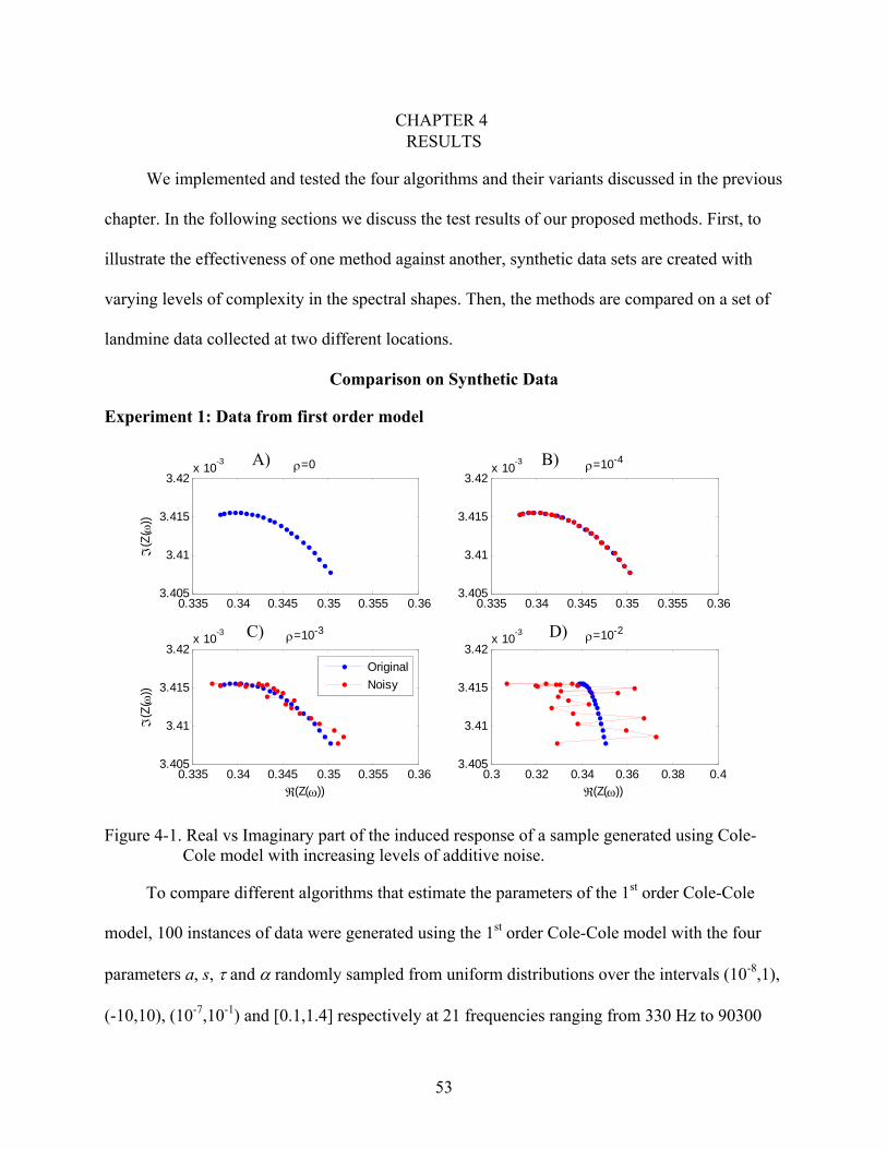
53
CHAPTER 4 RESULTS
We implemented and tested the four algorithms and their variants discussed in the previous
chapter. In the following sections we discuss the test results of our proposed methods. First, to
illustrate the effectiveness of one method against another, synthetic data sets are created with
varying levels of complexity in the spectral shapes. Then, the methods are compared on a set of
landmine data collected at two different locations.
Comparison on Synthetic Data
Experiment 1: Data from first order model
Figure 4-1. Real vs Imaginary part of the induced response of a sample generated using Cole-Cole model with increasing levels of additive noise.
To compare different algorithms that estimate the parameters of the 1st order Cole-Cole
model, 100 instances of data were generated using the 1st order Cole-Cole model with the four
parameters a, s, τ and α randomly sampled from uniform distributions over the intervals (10-8,1),
(-10,10), (10-7,10-1) and [0.1,1.4] respectively at 21 frequencies ranging from 330 Hz to 90300
0.335 0.34 0.345 0.35 0.355 0.363.405
3.41
3.415
3.42x 10⁻³ ρ=10-3
ℑ(Z
( ω))
ℜ(Z(ω))
0.335 0.34 0.345 0.35 0.355 0.363.405
3.41
3.415
3.42x 10⁻³ ρ=0
ℑ(Z
( ω))
0.335 0.34 0.345 0.35 0.355 0.363.405
3.41
3.415
3.42x 10⁻³ ρ=10-4
0.3 0.32 0.34 0.36 0.38 0.43.405
3.41
3.415
3.42x 10⁻³ ρ=10-2
ℜ(Z(ω))
OriginalNoisy
A) B)
C) D)

54
Hz in log scale. These were typical values seen in the landmine detection framework. The
experiments were repeated with zero mean Gaussian noise of variance σ2(ω) added at each
frequency. More precisely, the noisy versions of the signal are given by,
( ) ( ) ( )[ ] ( )[ ]( )∑=
ℑ+ℜ=+=fN
kkkN
1
222 where),0(' ωωρσσωω zzzz , with ρ = [10-4,10-3,10-2].
The effect of additive noise on the signal is shown by Argand diagrams in Figure 4-1. we
see that ρ = 10-3 was the point where noise started dominating the signal.
Observations
Figure 4-2 shows the fitting error as a function of the signal energy for different parameter
estimation methods. The circle fitting method by Bishay [9] worked well and was the fastest
method in the noise free case. However its performance degraded quickly in the presence of
noise. Figure 4-3 and Figure 4-4 compare the estimated values in the y axis to the true values in
the x axis. Therefore, a good estimate should lie on the y = x line. Figure 4-3 shows that even for
a low fitting error, the estimated parameters might be far from the true underlying parameters. It
also shows that in noise free case, the estimation of the parameter α was to be the least reliable
one. GRANMA produced the most robust results for noise levels up to ρ = 10-3. When ρ = 10-2,
all methods fail most of the time.
The experiments were carried out in MATLAB on a Linux based server with 10GB
memory and quad-core processor with each core operating at 2Ghz. Bishay’s circle fitting
method was the fastest with speeds about 10x faster than GRANMA which was in turn faster
than the iterative least squares method by 10x - 20x. The Xiang inversion method varied in speed
from 2x – 10x slower than GRANMA , depending on the number of iterations it required to
converge.

55
Figure 4-2. Fitting Error vs. Signal Energy for different parameter estimation methods of Cole-Cole model at different noise levels.
Figure 4-3. Actual vs. estimated parameter values for different Cole-Cole parameter estimation methods in the noise free case.
10-30 10-20 10-10 10010-30
10-20
10-10
100
||Z||
Fitti
ng E
rror
ρ=0
10-10 10-5
10-10
100
||Z||
Fitti
ng E
rror
ρ=10-4
10-10 10-5
10-5
100
||Z||
Fitti
ng E
rror
ρ=10-3
10-10 100
10-5
100
||Z||
Fitti
ng E
rror
ρ=10-2
granmaBishayXiang
10-10 10-5 10010-20
10-10
100 τ
Est
imat
ed
0 0.5 1 1.50
0.5
1
1.5α
-2 -1 0 1 2-2
0
2atan(s)
Est
imat
ed
Actual10-10 10-5 100
10-20
10-10
100
Actual
A
ActualgranmaXiangBishay
a

56
Figure 4-4. Actual vs. estimated parameter values for different Cole-Cole parameter estimation methods when ρ = 10-4. GRANMA produced the most robust estimates and Bishay and Xiang methods started to degrade in performance
Experiment 2: Comparison of Joint Sparse Methods on Data from second order model
The methods discussed in the previous experiment assume that the data come from a 1st
order Cole-Cole model. In most practical applications, the spectral shape of the data follows
higher order models. For example, we observed most low metal anti-personnel mines in our data
set exhibit behavior that is best described by a 2nd or 3rd order Cole-Cole model. In this
experiment, we compared the different dictionary search methods to simultaneously estimate the
order of the model along with the parameters of the model. The objective functions for the
different algorithms seek to produce models that accurately represent a set of observations with a
small number of dictionary elements.
To test this property, 100 different synthetic data sets were created using the same
procedure. A dictionary was created by varying τ and α in the range (10-9, 10) and (0, 1). The
dictionary was pruned so that no two elements had correlation greater than 0.96. This dictionary
was used for all 100 trials. In each trial, a two-step process was used to generate synthetic data.
10-8 10-6 10-4 10-2 10010-20
10-10
100 τ
0 0.5 1 1.50
1
2α
-2 -1 0 1 2-2
0
2atan(s)
10-8 10-6 10-4 10-2 10010-20
100
1020A
ActualgranmaXiangBishay
a

57
First, two random dictionary elements were selected from an (almost) uniform distribution over
the pruned dictionary. They were restricted to have correlation less than 0.3. Then, a data set of
25 spatially sequential data vectors was then generated by varying the weights of the two
relaxations using two differentiated Gaussian shapes in the down-track direction. The parameter
estimation algorithms were then applied to the data for 50,000 iterations with high weight given
to the sparsity terms of the objective functions.
Figure 4-5. Histogram image of Number of terms vs. Fitting error for different dictionary search methods. From the top left to the bottom right, A) L2 error with iterative reweighted L2 regularization, B) approximate L1 error with iterative reweighted approximate L1 regularization, C) quadratic programming with iterative reweighted L1 regularization, D) linear programming with iterative reweighted L1 regularization, E) quadratic programming with fixed L1 regularization, F) linear programming with fixed L1 regularization.
To compare the effectiveness of the algorithms, the histograms of fitting errors for
different numbers of nonzero terms is plotted in Figure 4-5. The plots are created by first plotting
F) L
fitting error
# of
term
s
0 2 4
5
10
15
E) Q
fitting error
# of
term
s
0 2 4
5
10
15
D) L IR
fitting error
# of
term
s
0 2 4
5
10
15
C) Q IR
fitting error#
of te
rms
0 2 4
5
10
15
B) L1
fitting error
# of
term
s
0 2 4
5
10
15
A) L2
fitting error
# of
term
s
0 2 4
5
10
15
0
5
10
15

58
parametric curves for each trial. Each curve plots number of nonzero rows of the weight matrix
vs. fitting error and the parameter is the iteration index. Histograms are then created by
overlaying all the parametric curves in one plot and counting how many times each cell is
covered. Here we observed that our L1 and L2 based methods outperformed off the shelf
quadratic and linear programming methods.
Experiment 3: Comparison of Cole-Cole and DSRF Dictionaries
In this experiment, the effect of choosing the right model to form the dictionary was
studied. Two dictionaries were designed based on the DSRF (α = 1) and Cole-Cole (α not
necessarily 1) models respectively. We refer to these two dictionaries as the DSRF and Cole-
Cole dictionaries. The maximum correlation between elements was restricted to 0.96 and both
had 11 elements each. This experiment had two parts: (1) synthetic data were generated from
the Cole-Cole model and α not close to 1 and (2) synthetic data were generated from the DSRF
model. In each part, we compare the two dictionaries by analyzing their convergence (using the
L1_IR method) to the correct number of parameters and the closeness to the true parameters. As
before, each part of the experiment consisted of 100 trials.
In part (1), data were generated for each trial by sampling the number of relaxations from a
uniform distribution over {1, 2, 3}. Once the number of relaxations was selected, then that
number of relaxations was sampled by sampling τ and α uniformly over the intervals (10-7, 1)
and (0.2, 0.8) respectively. The relaxations were combined using a preset combination of weights
to generate 25 data vectors as in the previous experiment. Gaussian noise with 10% of the energy
in the signal was added. Since both DSRF and Cole-Cole dictionaries used the same number of
elements, this experiment compares the effect of offsets in the τ and α spaces respectively. The
convergence statistics are given in Table 4-1.

59
Table 4-1. Comparison of convergence statistics: Part (1).
Dictionary
Convergence to
true number of
relaxations
Converged to the
closest
relaxations in the
parameter space
Converged to
relatively closer
distance in the
parameter space
Performed the
same
Cole-Cole 47% 0% 38% 53%
DSRF 9% 0% 9%
The meanings of columns two and three seem clear. The fourth and fifth columns of Table
4-1 require some discussion. The spacing between dictionary elements in the parameter space
varies non-uniformly because the parameter quantization depends on the correlation between the
elements. The spacing must be taken into account when calculating distance between the true
and estimated parameters since no algorithm can overcome the inherent quantization error. More
discussion of this will be given later. The fourth column measures the percentage of trials for
which each algorithm was closer to the true parameter set. The fifth column is the percentage of
cases for which they both the same distance from the true parameters. The DSRF dictionary
based method converged to the true number of relaxations only 9% of the time compared to the
Cole-Cole dictionary based method which converged 47% of the time.
In the second part, it was required that α = 1. Data were then generated in each trial with
one, two or three relaxations with τ uniformly sampled over the interval (10-7, 1) as described in
part (1). As can be seen in Table 4-2, both dictionaries produce the correct number of
relaxations but the DSRF errors are smaller more often. This should be expected because the
quantization in the line α = 1 is coarser for Cole-Cole than DSRF.

60
Table 4-2. Comparison of convergence statistics: Part (2)
Dictionary
Convergence to
true number of
relaxations
Converged to the
closest
relaxations in the
parameter space
Converged to
relatively closer
distance in the
parameter space
Performed the
same
Cole-Cole 100% 5% 15% 10%
DSRF 100% 21% 69%
Experiment 4: Dictionary update
The previous experiment assumed that the sample z is truly a linear combination of one or
more of the dictionary elements. This however is not practical as the correlation between
elements dictates the size of the dictionary and hence its resolution in the parameter space.
Therefore, in this experiment the dictionary is adapted to the data using the adaptive kernel
matching pursuit approach described in the technical approach. In this experiment, two
relaxations were used for every trial. They were selected by sampling τ and α uniformly over
the intervals (10-7, 1) and (0, 1) respectively. Figure 4-7 (f) is interesting. Each different colored
curve represents the distance of a particular dictionary element from the nearest true relaxation in
the parameter space. At the iteration for which a dictionary element is pruned, the curve ceases
since that element is no longer part of the solution. By the end of the iterations, there are only
two curves remaining, each of which have distance value almost zero. Thus, the algorithm
converges to the true relaxations and only the true relaxations.

61
Figure 4-6. Convergence diagnostics for dictionary search and update. From the top left to the bottom right plotted against iteration number, (a) L1 error, (b) iterative reweighted L2 regularization, (c) loss function with error and regularization terms combined, (d) total change in weights, (e) rate parameter of hyperbolic tangent controlling L1 approximation, (f) distance between true relaxations and dictionary elements in parameter space.
Experiment 5: Double Dictionary search – Proof of concept
To prove the concept of using double dictionary search we generated data with 2
relaxations taken from a dictionary of 23 elements. A down-track shape dictionary of 100
Gaussian pulses with different means and variances is designed with each pulse of duration 49
samples. This led to a total of 49 observations with their relaxations changing according to two
opposing Gaussian pulse shaped signals with means at locations 22 and 32 respectively. Zero
mean Gaussian random noise with 10% relative energy compared to the signal is added to the
data to test the robustness of the estimates.

62
Figure 4-7. Weights of individual relaxations using double dictionary search. The
estimated values are noisy versions of the original shape.
Figure 4-8. Two nonzero rows of the weight matrix WT showing row sparsity and nonzero values in columns corresponding to the down-track shape element.
Figure 4-7 and Figure 4-8 show that the results are accurate. This shows that a dictionary
of down-track shapes for objects of interest can be designed for a given sensor configuration.
Since this method is highly specific to data sets with particular sensor configurations, it is
reserved for future work.

63
Experiment 6: Dictionary Correlation Analysis
The effectiveness of any dictionary based search depends on the correlation between its
elements. This is because most dictionary search methods use the L2 norm of the fitting error.
Since the data and the elements are normalized to have a unit L2 norm, the fitting error becomes
dependant only on the correlation. Therefore, in an L2 norm based solution, two elements with
high correlation between them are almost indistinguishable.
Figure 4-9. Correlation regions of a Cole-Cole dictionary region. The black asterisks represent the DSRF dictionary elements chosen. Each of the different colors represent the regions that have 0.96 correlation or more with at least one or more of the dictionary elements. None of the dictionary elements can be used.
Figure 4-9 shows the regions in the Cole-Cole parameter space that are correlated with the
DSRF dictionary elements. This plot demonstrates that the Cole-Cole dictionary must be coarser
along the line α = 1 or else no dictionary elements with α ≠ 1 can be used.
10-10 10-8 10-6 10-4 10-2 100 1020.1
0.2
0.3
0.4
0.5
0.6
0.7
0.8
0.9
1
α
τ

64
Comparison on Landmine Data
Data Sets
The experiments were performed on two data sets. Each data set contains measurements
over buried mines, buried clutter objects and blanks. The first set contains 62 different types of
objects including 26 different types of mines collected over 11 adjoining lanes divided into 220
grid cells. The second set contains 24 different types of objects including 12 different types of
mines collected over 12 adjoining lanes divided into 225 cells. Table 4-1 shows the distribution
of objects in the data. The data were collected in two opposite directions over the same set of
grid locations using a Wideband EMI sensor developed by W. Scott [14]. The object is assumed
to be at the center of the grid cell and position errors were fixed manually.
Table 4-3. Nomenclature and Proportion
Notation Meaning Proportion
Set 1 Set 2 Total
HMAP High Metal Anti-Personnel mine 10% 3.6% 6.7%
LMAP Low Metal Anti-Personnel mine 21.4% 8.4% 14.8%
HMAT High Metal Anti-Tank mine 3.6% 1.3% 2.4%
LMAT Low Metal Anti-Tank mine 15.9% 6.2% 11%
HMC High Metal Clutter 15.5% 24.9% 20.2%
MMC Medium Metal Clutter 0% 12.4% 6.3%
LMC Low Metal Clutter 0% 12.4% 6.3%
NMC Non-Metallic Clutter or Blank 33.6% 30.7% 32.1% In the first data set, each grid cell is of dimension 1.5m x 1.5m and in the second one; they
are 1m x 1m. The WEMI sensor collects complex responses in 21 frequencies at 1cm intervals in
3 channels. This results in a 21 x 3 x 150 or 21 x 3 x 100 complex data matrix for each cell.

65
Data Filtering
Figure 4-10. Down-track filter template
The measured data are filtered in the down-track direction by convolving with a zero mean
template shown in Figure 4-10. This is used to remove ground response and sensor drift and also
to improve signal to noise ratio. Filtered data is used in our experiments for classification of
objects modeled with a 1st order Cole-Cole model. Only the data from the center channel and at
the center of the cell is used. This makes the first data set of size 220 grid cells x 2 directions and
the second data set of size 225 x 2. Unfiltered data is used in dictionary based feature extraction
methods as it represents the underlying physical phenomenon better.
Experiment 6: Classification of objects using first order model
Experiment setup
A 10 fold cross-validation was performed. Care was taken to avoid having the same cell
represented in both training and test sets simultaneously. To get fair representation of all objects
in the training data, object stratification was used to create the training and testing folds. This
method groups objects by type and splits them equally in all folds.
0 5 10 15 20 25-0.08
-0.06
-0.04
-0.02
0
0.02
0.04
0.06
0.08

66
Experiments and observations
The experiments were carried out for different algorithms in their increasing order of
complexity.
PRAM analysis
In this approach, first the gradient angles were computed for each grid cell. Since there are
28 different mines are in the data, one prototype per mine type was created from the training data
as per Equation 3-2. The non-mines were considered as outliers and not given prototypes. This
led to a one class classification approach with a test sample belonging to the mine class with
confidence given by Equation 3-3.
GRANMA analysis
Figure 4-11 plot showing the relationship between τ, α and EL for different mine types.
10-8 10-6 10-4 10-2 100 102
0
0.5
1
1.5100
105
1010
τ
α
EL
HMATHMAPLMATLMAP

67
In this approach, the landmine data were assumed to follow first order Cole-Cole models
and the parameters were extracted using GRANMA. The lookup table estimates of τ and α for
these data sets are shown in Figure 4-11. We have already seen from Figure 3-3 and the
corresponding section that, the error surface and the update gradients are highly nonlinear
especially near regions where ωτ = 1 and α ≈ 2. But, Figure 4-12 shows that searching for α
between 0.1 and 1.4 (in linear scale) and for τ in the range of 10-6 to 1 (in log scale) was
sufficient for the data in the present experiments. This justifies the choice of using a lookup table
method. Future research may be targeted towards using alternative methods to a lookup table
such as regression and direct inversion.
Figure 4-12. τ and α for different object types.
The features are log10(Α), s, log10(τ), α, log10(EL) and EF making a feature set of size 220 x
2 for the first data set and of size 225 x 2 for the second data set.
1000
0.5
1
HMAT
α
1000
0.5
1
HMAP
1000
0.5
1
LMAT
1000
0.5
1
LMAP
1000
0.5
1
HMC
α
τ100
0
0.5
1
MMC
τ100
0
0.5
1
LMC
τ100
0
0.5
1
NMC
τ

68
⎥⎦
⎤⎢⎣
⎡= F
L Es
sA
AE
EFmaxmax
10
max
10
maxmax
10 ˆ)ˆ(log)(logˆ)ˆ(log
vectorFeature
αα
ττ
(4-1)
where Amax, smax, τmax, αmax and Emax are scaling parameters.
Figure 4-12 shows that for different object types form their own clusters in the (α, τ) space
whereas non-metallic clutter (NMC) is spread all over. This is because there is no specific region
in the lookup table that matches with NMC.
Bishay method and Xiang inversion analysis
In this approach, the landmine data was assumed to follow first order Cole-Cole model and
the parameters were extracted using Xiang inversion and Bishay method and the classification is
done using the same soft kNN method described for GRANMA.
Feature Selection
Since the Xiang inversion and Bishay method produced 5 features and GRANMA
produced 6 features, each algorithm is evaluated for all its feature subsets. This makes 26-1 = 63
classification experiments for GRANMA and 25-1 = 31 experiments each for the Bishay method
and Xiang inversion method. The results are compared using best ROC curves.
Observations
GRANMA outperformed the other Cole-Cole feature extraction methods in terms of
classification accuracy while Bishay method was the fastest. Even though all methods estimated
the same features and used same type of classifier, the consistency in parameter estimates
contributed to the difference in performance.

69
Figure 4-13. ROC curves of different landmine detection algorithms with their corresponding best features. ErrLookup and ErrFit denote the lookup table error and the fitting error respectively as defined in Equation 3-8 and Equations 3-11.
Experiment 7: Analysis of GRANPA on landmine data
Figure 4-14. Change in Argand diagram with distance for a Low Metal Anti-Personnel Mine buried at 1”.
0 0.1 0.2 0.3 0.4 0.5 0.6 0.7 0.8 0.9 10
0.1
0.2
0.3
0.4
0.5
0.6
0.7
0.8
0.9
1
PFA
PD
ROC Curves
PRAM
GRANMA: tau c ErrLookup A s
Xiang: tau c A ErrFit
Bishay: tau c A s ErrFit
Xiang
PRAM
Bishay GRANMA α
α α

70
Figure 4-15. Change in amplitude with distance for a Low Metal Anti-Personnel Mine buried at 1”. The location nearest to the object is noted by the blue ellipse. The x axis denotes observation number along down track
Figure 4-14 shows the variation in the spectral shape of unfiltered data as measurements
are taken at increasing distance from the object. GRANMA and other first order approximation
methods model the far field well and produce consistent parameter estimates for different
instances of the same type of object. However, in the near field, data looks more piecewise first
order. Figure 4-15 shows the variation in amplitude with distance. It shows that the amplitude
crosses zero closest to the object. Also, the observation closest to the zero crossing shows the
maximum near field effect. Therefore GRANPA was used to extract parameters from the
observation closest to the zero crossing and used to initialize an iterative search procedure to
connect the parameters of near and far field. This iterative schedule is summarized in the
following pseudo-code
GRANPA_ILS
1. Find zero crossing location d0 2. Choose either positive or negative amplitude side 3. Estimate order and parameters using GRANPA S0 4. CurrentObservation← Start of Positive Amplitude Side 5. Sstart ← S0 6. while CurrentObservation < EndOfPositiveAmplitudeSide
a. CurrentObservation ← Move to next observation b. Use iterative least squares with initial conditions Sstart

71
c. Sstart ← New solution 7. end while 8. CurrentObservation← Start of Negative Amplitude Side 9. Sstart ← S0 10. while CurrentObservation > BeginningOfNegativeAmplitudeSide
a. CurrentObservation ← Move to previous observation b. Use iterative least squares with initial conditions Sstart c. Sstart ← New solution
11. end while
Figure 4-16. Change in parameter values for a second order approximation estimated using GRANPA. The x axis denotes observation number along down track. The amplitude zero crossing happens at observation number 90.
Figure 4-16 shows that as the distance from the object increases, the parameter values
change. While it is expected that the amplitude and the shift can change with distance, the values
of τ and α should not as they are dielectric properties of the object under study.
70 80 90 100110
-5
-4.5
τ1
70 80 90 100 1100.850.9
0.951
1.05
α1
80 100-1
0
1x 10⁻⁵ A1
80 100
0.3
0.4
0.5
s1
80 100-7
-6
-5
τ2
80 100
0.81
1.2
α2
80 100-4-2024
x 10-5 A2
80 1000.60.8
11.2
s2
80 100
-1
0
1
x 10-5A1s1+A2s2

72
Experiment 8: Analysis of Dictionary methods on landmine data
Figure 4-17. Parameter values estimated using DSRF along down-track. The x axis denotes distance along down track. The amplitude zero crossing happens at location 0.8m from the start. The horizontal lines correspond to parameters estimated using joint sparse optimization.
Figure 4-17 shows the difference between individual and joint sparse optimization using
DSRF. Without the joint sparsity constraint, the dictionary elements selected at different
locations are free to change.

73
Figure 4-18. Parameter values estimated using joint sparse DSRF along down-track. The x axis denotes observation number along down track. The y axes denote the weight of corresponding dielectric relaxations. The amplitude zero crossing happens at observation number 35 from the start of the segment
Figure 4-18 shows DSRF parameters estimated on a segment of the same data using a joint
sparsity constraint. This constrains the τ values to be constant along the down-track and only the
amplitudes of the relaxations change

74
Figure 4-19. Relaxations estimated using a Cole-Cole dictionary on the left vs. those estimated
using a DSRF dictionary. The x axis corresponds to different cell locations for the same mine type.
Figure 4-20. Usage of dictionary elements by the landmine data. We want similar mines to use the same dictionary elements and hence lesser number of them.
Joint Sparse Cole-Cole
101-S 102-J 104-N 106-H 109-E 109-K
1+0i0+1i
alpha=0.5 tau=10 -̂9alpha=0.7 tau=10 -̂9alpha=0.9 tau=10 -̂9
alpha=0.1 tau=10 -̂8.9alpha=1 tau=10 -̂5.6
alpha=0.9 tau=10 -̂5.3alpha=0.6 tau=10 -̂5.2
alpha=1 tau=10 -̂4.9alpha=0.7 tau=10 -̂4.7
alpha=1 tau=10 -̂4.4alpha=1 tau=10 -̂4.1
alpha=0.9 tau=10 -̂3.6alpha=1 tau=10 -̂3.3
alpha=0.3 tau=10 -̂2.7alpha=1 tau=10 -̂2.6
alpha=0.6 tau=10 -̂1.9
Joint Sparse DSRF
101-S 102-J 104-N 106-H 109-E 109-K
1+0i0+1i
tau=10 -̂7.2tau=10 -̂6.6tau=10 -̂6.3tau=10 -̂6.1tau=10 -̂5.9tau=10 -̂5.7tau=10 -̂5.2tau=10 -̂4.7tau=10 -̂4.5tau=10 -̂4.3tau=10 -̂4.1tau=10 -̂3.9tau=10 -̂3.7tau=10 -̂3.5tau=10 -̂3.3tau=10 -̂3.1
0 2 4 6 8 10 12 14 16 18 200
50
100
150
dictionary index
# of
tim
es u
sed
Cole-Cole dictionary
0 2 4 6 8 10 12 14 16 18 200
50
100
150
dictionary index
# of
tim
es u
sed
Debye dictionary
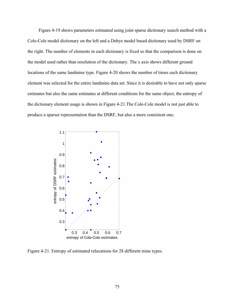
75
Figure 4-19 shows parameters estimated using joint sparse dictionary search method with a
Cole-Cole model dictionary on the left and a Debye model based dictionary used by DSRF on
the right. The number of elements in each dictionary is fixed so that the comparison is done on
the model used rather than resolution of the dictionary. The x axis shows different ground
locations of the same landmine type. Figure 4-20 shows the number of times each dictionary
element was selected for the entire landmine data set. Since it is desirable to have not only sparse
estimates but also the same estimates at different conditions for the same object, the entropy of
the dictionary element usage is shown in Figure 4-21.The Cole-Cole model is not just able to
produce a sparser representation than the DSRF, but also a more consistent one.
Figure 4-21. Entropy of estimated relaxations for 28 different mine types.
0.3 0.4 0.5 0.6 0.7
0.3
0.4
0.5
0.6
0.7
0.8
0.9
1
1.1
entropy of Cole-Cole estimates
entro
py o
f DS
RF
estim
ates

76
CHAPTER 5 CONCLUSIONS
We have developed four algorithms to detect, analyze and identify objects using wideband
electromagnetic induction data. The first and simplest PRAM method is quick and doesn’t make
any assumptions about the data. It removes the variability in the amplitude and drifts in the data
and has been found to be useful in designing a pre-screener to mark interesting sections of
ground for further analysis. The second method GRANMA gives a robust way of estimating the
Cole-Cole parameters and provides consistent features that can be used for object classification.
The third method GRANPA uses the same framework as GRANMA and is a quick way of
modeling near field effects. The fourth method SPARDIR separates the sensor setup from the
dielectric properties of objects and provides a framework to study them.
Future work may be targeted towards speeding up GRANMA by searching only a section
of the lookup table using the range of the gradient angles. More statistical analysis on the
convergence of the developed L1 version of SPARDIR needs to be done. Another area of
promise is using SPARDIR to extract features identify objects.

77
LIST OF REFERENCES
[1] H. Huang and I.J. Won, “Identification of Mineral Deposits using Airborne Electromagnetic Spectra”, Expanded Abstracts, Society of Exploration Geophysics, pp. 5-8, 2002.
[2] M Gourzi, A Rouane, R Guelaz, M Nadi, M Alavi and M McHugh, “Non-invasive Glycaemia Blood Measurements by Electromagnetic Sensor: Study in Static and Dynamic Blood Circulation”, Journal of Medical Engineering and Technology vol. 27 (1), pp. 22–26, 2005.
[3] A. Ghorbani, C. Camerlynck, N. Florsch, P. Cosenza and A. Revil, “Bayesian Inference of the Cole-Cole Parameters from Time and Frequency-domain Induced Polarization”, Geophysical Prospecting, 55(4), 589–605. doi:10.1111/j.1365-2478.2007.00627.x.
[4] C. Bruschini, “A Multidisciplinary Analysis of Frequency Domain Metal Detectors for Humanitarian Demining”, PhD thesis, Vrije Universiteit Brussel (VUB), September 2002.
[5] J. Miller, T. H. Bell, J. Soukup and D. Keiswetter, “Simple Phenomenological Models for Wideband Frequency-Domain Electromagnetic Induction”, IEEE Trans. on Geoscience and Remote Sensing, vol. 39, pp. 1294-1298, June 2001.
[6] T. H. Bell, B. Barrow, J. Miller and D. Keiswetter, “Time and Frequency Domain Electromagnetic Induction Signatures of Unexploded Ordnance”, Subsurface Sens. Tech. Appl. 2(3): pp. 153-175, 2001.
[7] C.E. Baum, Ed., Detection and Identification of Visually Obscured Targets, New York: Taylor & Francis, 1999.
[8] K. S. Cole and R. H. Cole, “Dispersion and Absorption in Dielectrics, I. Alternating Current Characteristics”, J. Chem. Phys, 1, pp 341-351, 1941
[9] S. T. Bishay, “Numerical Methods for the Calculations of Cole-Cole parameters”, Egypt J. Solids, vol. 23, pp 179-188, 2000.
[10] W. H. Pelton, P. G. Ward, W. R. Sill and P. H. Nelson, “Mineral Discrimination and Removal Inductive Coupling with Multifrequency IP”, Geophysics, vol. 43, 588-609, 1978.
[11] J. Xiang, N. B. Jones, D. Cheng and F. S. Schlindwein, “Direct Inversion of the Apparent Complex-resistivity Spectrum”, Geophysics, vol. 66, pp. 1399-1404, 2001.
[12] M. Wei, W. R. Scott and J. H. McClellan, “Robust Spectrum of the Discrete Spectrum of Relaxations for Electromagnetic Induction Responses”, IEEE Trans. on Geoscience and Remote Sensing, to be published.
[13] S. Gabriel, R. W. Law and C. Gabriel, " The Dielectric Properties of Biological Tissue: III. Parametric Models for the Dielectric Spectrum of Tissues," Phys. Med. Biol., vol. 14, pp. 2271-2293, 1996.

78
[14] E. Fails, P. Torrione, W. Scott, L. Collins, “Performance of a Four Parameter Model for Landmine Signatures in Frequency Domain Wideband Electromagnetic Induction Detection Systems”, Proc. SPIE, Detection and Remediation Technologies for Mines and Mine-like Targets XII; Russell S. Harmon, J. Thomas Broach, John H. Holloway, Jr.; Eds., vol. 6553, 2007.
[15] S. E. Yuksel, G. Ramachandran, P. Gader, J. Wilson, D. Ho, and G. Heo, “Hierarchical Methods for Landmine Detection with Wideband Electro-magnetic Induction and Ground Penetrating Radar Multi-sensor Systems,” Int.l Geoscience and Remote Sensing Symposium (IGARSS), vol. 2, pp. II-177 – II-180, July 2008.
[16] D. L. Donoho and M. Elad, “Optimally Sparse Representation in General (Nonorthogonal) Dictionaries via ℓ1 Minimization,” Proc. Nat.l Academy of Sciences of the United States of America, vol. 100 (5), pp. 2197-2202, March 2003.
[17] J. Chen and X. Huo, “Theoretical Results on Sparse Representations of Multiple-measurement Vectors”, IEEE Trans. on Signal Processing, vol. 54 (12), pp 4634-4643, December 2006.
[18] S. Foucart, and M.J. Lai, “Sparsest Solutions of Underdetermined Linear Systems via Lq Minimization for 0 < q < 1,” Applied and Computational Harmonic Analysis, vol. 26 (3), pp 395-407, 2009.
79
BIOGRAPHICAL SKETCH
Ganesan Ramachandran received the Bachelor of Engineering degree in Electronics and
Communication Engineering from the Regional Engineering College, Tiruchirappalli, Tamil
Nadu, India in May 1999. He received his Master of Science and Doctor of Philosophy degrees
in Electrical and Computer Engineering from the University of Florida in August 2002 and May
2010 respectively.
Currently, he is a research assistant in the Computational Science and Intelligence Lab in
the Computer and Information Sciences and Engineering Department at the University of
Florida. Research includes the development of algorithms, methodologies, and models with a
solid mathematical and/or statistical base with applications to landmine detection. Current and
previous research applies these methods to a variety of data including electromagnetic induction,
radar, weather and biomedical.