Embed Size (px)
Citation preview

FAST POWER NETWORK DETECTION OF TOPOLOGY CHANGE LOCATIONS
USING PMU MEASUREMENTS
By
Elamin Ali Elamin Mohamed
Ahmed H. Eltom Abdelrahman A. Karrar
Professor of Electrical Engineering Professor of Electrical Engineering
Committee Chair Committee Co-Chair
Gary L. Kobet
Adjunct Professor of Electrical Engineering
Committee Member

ii
FAST POWER NETWORK DETECTION OF TOPOLOGY CHANGE LOCATIONS
USING PMU MEASUREMENTS
By
Elamin Ali Elamin Mohamed
A Thesis Submitted to the Faculty of the University of
Tennessee at Chattanooga in Partial Fulfillment
of the Requirements of the Degree of
Master of Science: Engineering
The University of Tennessee at Chattanooga
Chattanooga, Tennessee
December 2016

iii
ABSTRACT
System monitoring and contingency analysis are crucial functions in power control
centers. These applications need a complete model of the power network to perform the desired
analysis. Yet, this model must be continuously updated to account for system dynamics. Several
topology processing schemes have been developed to accomplish this task. The majority of these
schemes process breaker statuses to detect changes in system topology which results in a
complicated analysis method.
In this work, a simple and quick method for on-line detection and identification of system
topology changes using PMU measurements is introduced. This method is based on representing
line outages with fictitious nodal power injections. The algorithm can be applied on systems that
are not entirely covered by PMUs.
The scheme was tested during different outage events in the IEEE39-bus system. The
obtained results validated the algorithm’s ability to detect and identify line outage events
effectively and efficiently.

iv
TABLE OF CONTENTS
ABSTRACT ................................................................................................................................... iii
TABLE OF CONTENTS ............................................................................................................... iv
LIST OF TABLES ......................................................................................................................... vi
LIST OF FIGURES ...................................................................................................................... vii
CHAPTER
1. INTRODUCTION ........................................................................................................ 1
1.1 BACKGROUND ....................................................................................................................... 1 1.2 PROBLEM STATEMENT .......................................................................................................... 1 1.3 OBJECTIVES ........................................................................................................................... 2 1.4 STUDY OUTLINE .................................................................................................................... 2
2. LITERATURE REVIEW ............................................................................................. 3
2.1 INTRODUCTION ...................................................................................................................... 3
2.2 CONVENTIONAL TOPOLOGY PROCESSING SCHEMES ............................................................ 7
2.3 PMUS IN TOPOLOGY PROCESSING ........................................................................................ 9
2.3.1 Phasor Measurement Units ............................................................................................. 9
2.3.2 PMU-Based Topology Processing Schemes ................................................................. 10
3. METHODOLOGY ..................................................................................................... 13
3.1 INTRODUCTION .................................................................................................................... 13
3.2 BACKGROUND ..................................................................................................................... 13
3.3 NODAL INJECTIONS IN A SIMPLIFIED SYSTEM MODEL ........................................................ 15
3.4 COMPLETE ALGORITHM ...................................................................................................... 19
3.4.1 Determining the Event Area ......................................................................................... 20
3.4.2 Identifying the Outaged Element .................................................................................. 25
4. RESULTS AND DISCUSSION ................................................................................. 28

v
4.1 TEST SYSTEM DESCRIPTION ................................................................................................ 28
4.2 SIMULATION RESULTS ......................................................................................................... 29
4.2.1 Normal Operating Condition ........................................................................................ 29
4.2.2 Line Outage between Two Observed Buses ................................................................. 35
4.2.3 Outage Events in Unobserved Area .............................................................................. 40
4.2.3.1 Line Outage - Case Study A ................................................................................. 40
4.2.3.2 Line Outage - Case Study B .................................................................................. 43
4.2.3.2 Transformer Outage- Case Study C ...................................................................... 46
4.2.4 Other Outage Events ..................................................................................................... 47
5. CONCLUSION ........................................................................................................... 50
5.1 CONCLUSION ....................................................................................................................... 50
5.2 FUTURE WORK .................................................................................................................... 51
REFERENCES ............................................................................................................................. 52
APPENDIX A ............................................................................................................................... 53
VITA…….…………………………………………………………………………….…………59

vi
LIST OF TABLES
2.1 SCADA vs PMUs………………………………………………..…………………………..10
4.1 System states during normal operating conditions…………………..………………………30
4.2 Active and reactive line power flows…………………………………..……………………32
4.3 Active and reactive power injection errors during normal operating conditions……..……..34
4.4 System states during outage of line 28-29…………………………………..……………….35
4.5 Active and reactive power injection errors during outage of line 28-29…………..………...37
4.6 Active and reactive power injection errors after updating the topology with line 28-29
out…………………………………………………………………………………….….39
4.7 Active and reactive power injection errors during outage of line 21-22…………….…..…..40
4.8 Power transferred between event area boundaries and the rest of the system during line
21-22 outage event………………………………………………………………..….…..42
4.9 Active and reactive power injection errors when updating the topology with line
21-22 out……………………………………………………………………….……..….43
4.10 Active and reactive power injection errors during outage of line 10-11…….………..……43
4.11 Active power injection errors during trial-and-error process for case B…….……….….…45
4.12 Active and reactive power injection errors during outage of transformer T12………...…..46

vii
LIST OF FIGURES
2.1 Phasor angle measurements……………………………………………………………...…..11
3.1 (a) Line k before outage, (b) Line k after outage, (c) Simulating line k outage using
fictitious injections at buses n and m……………………………………..……………...14
3.2 (a) Two-Bus system with both lines in service, (b) One of the lines out of service,
(c) outaged line in service with power injections………………….……………….……17
3.3 7-bus system………………………………………………………………………………….22
3.4 Complete topology processing scheme………………………………………………………27
4.1 IEEE39-bus system……………………….………………………………………………….29
4.2 Bus-12 P-index during different operating conditions……………………………………….48

1
CHAPTER 1
1 INTRODUCTION
1.1 Background
Power system networks experience several dynamic events during operation. However,
network solution programs, such as the state estimator, need a correct and up-to-date
configuration of the system in order to perform their function. This necessitates the availability
of a mathematical model that incorporates the changing operating conditions of the system [1].
To accomplish this purpose, several topology processing schemes have been developed.
1.2 Problem Statement
Conventional topology processing schemes relies on communicated breaker status
information in order to configure the present system topology. However, these schemes
generally deploy a sophisticated logic to analyze and process this information and consequently
reflect the effect of breaker status changes on system configuration. The complexity of these
logics results in a considerable processing time [2]. This implies the need for developing a fast
and simple topology processing scheme.

2
1.3 Objectives
The objective of this work is to develop a fast and reliable scheme for detection of
topology change locations in power networks using PMU measurements. This scheme is to be
applied on reduced systems where parts of the network are not monitored using PMUs.
1.4 Study Outline
The remaining chapters of this thesis are organized as follows:
Chapter Two: in this chapter, topology processing schemes presented in the literature
are reviewed along with their merits and drawbacks.
Chapter Three: this chapter introduces the theory behind the proposed scheme.
Furthermore, a detailed description of the processes followed to detect and identify
topology change locations is provided.
Chapter Four: this chapter presents simulation results when testing the algorithm
performance on the IEEE39-bus system.
Chapter Five: this chapter discusses the contributions of this work in the area of
topology estimation and lists the advantages of the developed scheme.

3
CHAPTER 2
2 LITERATURE REVIEW
2.1 Introduction
A power system is said to be secure if it continues to operate despite components failure.
Power system security mainly consists of three major functions which are system monitoring,
contingency analysis and security-constrained optimal power flow.
System monitoring is achieved through gathering real time measurements from the field.
These telemetered measurements reflect the up-to-date condition of the network. Such
measurements along with their data transmission system are referred to as energy management
system (EMS). The EMS provides the means for monitoring system voltages, power flows,
circuit breakers statuses, etc. This tremendous amount of telemetered data implies the use of
digital computers in order to process and store them in a database. The data are then used to
perform state estimation [1].
State estimation is a process that uses system measurements to assign value to an
unknown system state depending on some criteria. The process usually deals with redundant
measurements, and estimates the true value of these states using certain statistical criteria.
Voltage magnitudes and their relative phase angles are considered to be the state variables in
power systems. The best estimate of these states depends on the available measurements. These
measurements could be voltage magnitudes, ampere-flow or power-flow quantities [1].

4
One of the most common approaches to perform state estimation is the weighted least-
square method. This method aims to minimize the overall squared difference between the
estimated state and the measured one. Equation (2.1) shows the function to be minimized.
𝐽 =∑𝑊𝑗|𝑋𝑚,𝑗 − 𝑋𝑐,𝑗|2
𝑀
𝑗=1
(2.1)
Where
𝑋𝑚,𝑗 = j-th measurement
𝑋𝑐,𝑗 = j-th calculated measurement
𝑊𝑗 = weighting factor for j-th measurement
M = number of measurements
The measurements fed to the state estimator must be combined with the corresponding
model of the system to generate an estimate of the present system states. This implies that the
system configuration must always be kept up-to-date [2].
Contingency analysis programs simulate potential system failures in order to alarm
system operators to any serious trouble which might cause cascading events. A complete model
of the power system is needed to perform this analysis. Furthermore, this system model must be
continuously updated to reflect current system conditions for the purpose of on-line analysis.
Topology processing schemes have been developed to accomplish this task. It is worth
mentioning that besides state estimation and on-line contingency analysis, up-to-date system

5
model is also used by many other applications. For example, it can enhance the economic
dispatch program by providing updated penalty factors [1].
The power system connectivity data is used to construct a model that can be used by the
aforementioned applications. These data are normally stored in terms of bus-sections and circuit
breakers. However, in order to perform these analyses, the data need to be expressed in terms of
buses and branches. Figure 2.1 shows an example of the transformation from a bus-
section/circuit-breaker model to a bus/branch form [3].
6
(a)
2 4
3
1GU1
SH1
TR1
LI2 LI3
LI1
LD1
LD2+LD3
(b)
Figure 2.1 (a) Bus-Section/Circuit Breaker Network Model, (b) Bus/Branch Network Model

7
2.2 Conventional Topology Processing Schemes
Conventional topology processing schemes use telemetered circuit breaker statuses along
with their connectivity data in order to determine the present system topology [3]. Whenever a
change in a breaker status occurs, the topology processor is reinitialized to update the existing
system model.
Several topology processing schemes were proposed in the literature. Reference [2]
established one of the schemes which serves as a foundation in this area. The authors proposed a
topology processing program that updates the configuration of substations based on breaker
status changes. The scheme assigns a number to each substation in the system starting from 1 on.
Moreover, transmission lines, transformers and system buses are also numbered in another
different sequence. The suggested algorithm starts by creating a table which contains the initial
data of circuit breakers. This table stores the two circuits between which a circuit breaker is
connected along with the initial status of the breaker. Another table is set up to indicate the
availability of transmission line measurements for load flow purposes. Real time data are then
collected from the system to detect any loss of measurements or breaker status changes in
substations. Such a scenario will trigger the algorithm to update system topology. The scheme
examines the substations in which circuit breaker status changes have taken place. The algorithm
logic essentially searches for all the closed paths within these substations. Multiple closed paths
within a substation indicate that the substation has been disconnected forming new nodes. These
nodes are then assigned new numbers with one node keeping the original number of the
substation before being split. Subsequently, system data tables are modified to include the new
formed nodes. Furthermore, the algorithm detects transmission lines and transformers which are

8
open at one or both ends due to changes in breaker statuses. The measurements of these circuits
are then excluded from subsequent load flow analysis. The scheme then proceeds to check
whether open lines or transformers have led to the isolation of some parts of the network,
creating islands. This process is similar to that followed when searching for closed paths within a
substation with lines and transformers being treated as if they were circuit breakers.
Transmission lines measurements belonging to areas which don’t have a reference voltage bus
are also excluded from subsequent analysis.
Although the contribution of this work is considered remarkable in the area of topology
processing, the algorithm suffers some major deficiencies [4]. First, it is considered to be time
consuming since a change within a substation will cause the algorithm to reassess the topology
of the whole system. Furthermore, the algorithm is triggered only by changes within substations
i.e. changes in transmission line breakers which are not located in a substation don’t cause
system topology modifications. The scheme assigns new numbers to nodes resulting from
substations splitting. These numbers are hard to trace when multiple events are encountered.
Moreover, the algorithm is not designed to deal with breaker closing events [4].
Authors of [5] proposed a topology processing scheme that is based on the work
presented in [2]. This latter method repeats topology processing whenever a change is detected
without consideration to the model resulting from the previous cycle. However, the method
suggested by Prais and Bose [5] makes advantage of the fact that major topology changes in
power networks are not frequent. Hence, it is not necessary to rebuild system matrices in each
cycle. Instead, the algorithm traces the changes in the bus/branch model and rebuilt system
matrices only when major changes have occurred. This would lead to an increase in the

9
execution time of the topology processing, but the overall computation time would be greatly
improved. It is to be noted however that this method suffers the same aforementioned
deficiencies of [2].
2.3 PMUs in Topology Processing
2.3.1 Phasor Measurement Units
Phasor measurement units (PMUs) are devices used to measure electrical waves namely,
voltages, currents and frequencies in a synchronized environment. The deployment of these
devices helps achieving better utilization of electrical measurements. PMU measurements are
presented in terms of magnitude and angle with a high sampling rate, typically 30 measurements
per cycle. Universal standard time is used to synchronize different PMU measurements from
various locations. One of the most effective devices to attain this time reference is the Global
Positioning System (GPS). Synchronized Measurements obtained from different PMUs are
called synchrophasors.
Legacy supervisory control and data acquisition (SCADA) systems provide vital
information for power network operators. The asynchronous nature of this information along
with the low sampling rate, compared to PMUs, makes it impossible for wide area monitoring
and control in real time environment [6]. This can be accomplished however with the
employment of PMUs. Table 2.1 presents a brief comparison between SCADA system and
PMUs [7].

10
Table 2.1 SCADA vs PMUs
FEATURE SCADA PMU
Sampling rate 1 sample every 2-10 Seconds
(steady State Monitoring)
1-60 samples per second (Dynamic
Monitoring)
Measurements Magnitude only Magnitude and phase angle
Time Synchronization No Yes
Employment Local monitoring and control Wide area monitoring and control
Synchrophasors obtained from different PMUs enable dynamic monitoring of the system.
Such a feature has paved the way for many initiative projects to improve power networks
performance. These projects aim to upgrade power systems operation, supervision, protection
and control [8].
2.3.2 PMU-Based Topology Processing Schemes
Many researches have been conducted to make use of PMU information to increase
situational awareness of power system operators. PMU data are being incorporated in
applications such as state estimation, visualization and dynamic security assessment [9].
However, only few researches focused on the use of PMU data for topology processing
enhancement. One of the prominent works in this area is presented by Tate and Overbye. The
suggested algorithm utilizes PMU phasor angle measurements along with transmission lines and
system connectivity data to detect single line outages on the network.

11
The scheme assumes that a certain number of busses are being observed using PMUs.
These buses are referred to as observable buses. Whenever an outage occurs on the system, the
phasor angles of the observed buses experience changes. The synchrophasor angle measurements
from these buses are low-pass filtered to eliminate transient oscillations. Figure 2.2 shows an
example of a PMU angle measurement and its filtered form. An edge detection method is then
used to detect changes in these measurements.
Figure 2.1 Phasor angle measurements
Where 𝜃𝑖 is the actual angle measurements, 𝜃𝑖,𝐿𝑃𝐹 is the filtered one and 𝑁𝑡𝑟𝑎𝑛𝑠 is the number of
samples over which a difference in steady state angles is calculated [9].
The algorithm uses DC power flow equations to express the angle changes in term of the
pre-outage flows on the lines as shown in equation (2.2).

12
∆𝜃 = 𝐵−1∆𝑃 (2.2)
Where ∆𝑃 is a vector of power injections changes on each bus due to line outage, B is the
susceptance matrix. The calculated angle changes together with the observed ones are then used
to form an optimization problem. The solution to this problem is the event that drives the
difference to be minimum as shown in equation (2.3)
Line outage 𝑙∗ = arg𝑚𝑖𝑛𝑙∈(1,2,…𝐿) |∆𝜃𝑜𝑏𝑠𝑒𝑟𝑣𝑒𝑑 − ∆𝜃𝑐𝑎𝑙𝑐𝑢𝑙𝑎𝑡𝑒𝑑| (2.3)
Where 𝑙 is the number of lines in service before the event [10].
Although this algorithm uses limited number of PMUs to detect line outages, it has some major
issues. Firstly, the adoption of DC load flow introduces errors in the calculations of the changes
in phasor angles. That is due to the fact that DC load flow conditions do not hold in real systems.
Moreover, the changes in phasor angles are not necessarily caused by line outages. Generator
outages for instance could also lead to such changes. Another point to consider is that the
algorithm will not be able to distinguish between different line outage events that cause similar
phasor angle changes. Furthermore, a moving window of samples must be set to include the
entire transition region in the case of an event. This will introduce a delay in the detection of
phasor angle changes.

13
CHAPTER 3
3 METHODOLOGY
3.1 Introduction
In this chapter, a new topology processing scheme which detects line outage events in
real time is presented. Unlike the methods described in chapter two which depends on breaker
status data, this method rather uses system state information along with nodal power
measurements obtained from PMUs to identify and locate line outages. Furthermore, the scheme
can be applied on reduced systems where system state data for unobserved buses is absorbed in
the aggregation.
3.2 Background
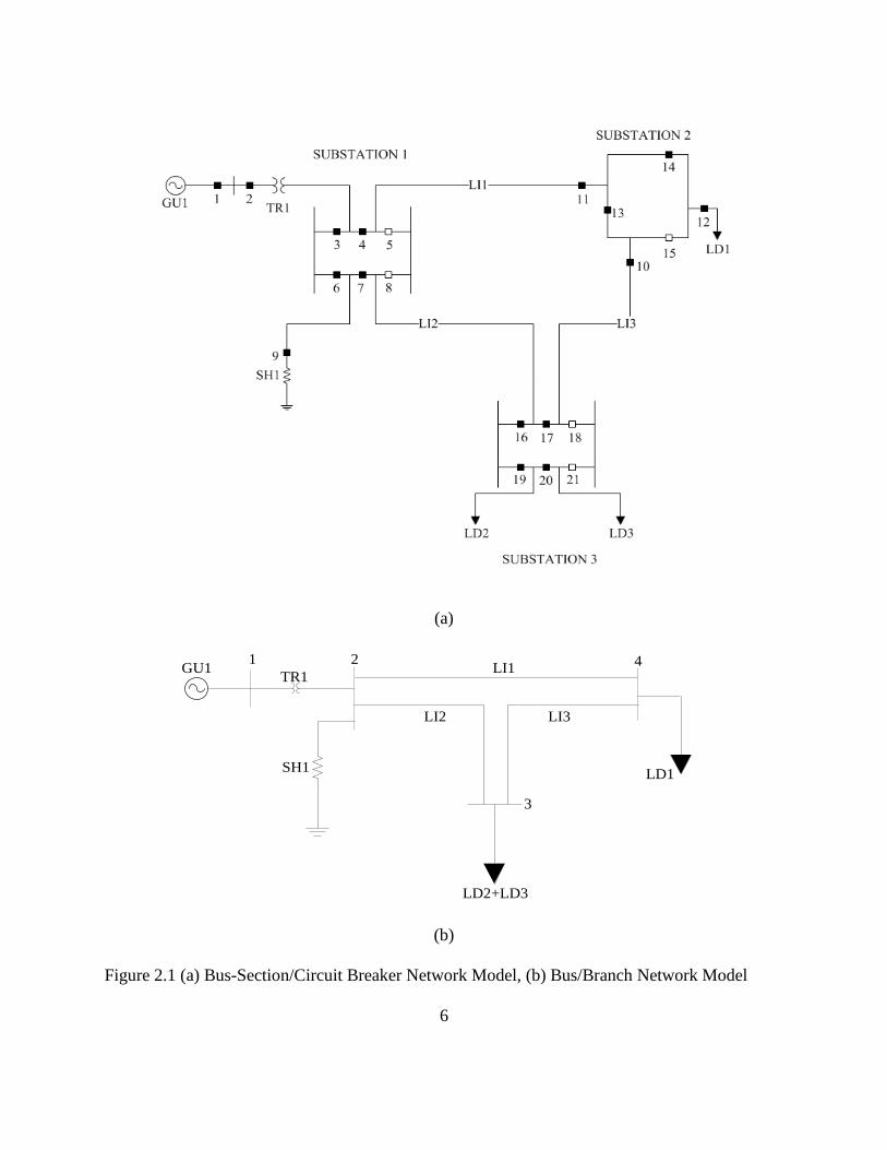
In [1], a method to simulate line outages without the need to update system topology was
developed. This method adds two fictitious injections into the buses between which the line was
connected. This can be demonstrated by referring to figure 3.1. Line k is connected to the system
through buses n and m. The original flow on the line is 𝑃𝑛𝑚. However, when the breakers at the
end of the line open, this flow goes to zero. This outage event can be simulated by adding
injections ∆𝑃𝑛 and ∆𝑃𝑚 at buses n and m respectively with both breakers closed. The will result
in a power �̃�𝑛𝑚 flowing in the line. To derive the flow at line breakers to zero, the injected power
at bus n should flow through line k and out of bus m. this implies that:
14
∆𝑃𝑛 = �̃�𝑛𝑚 3.1
∆𝑃𝑚 = −�̃�𝑛𝑚 3.2
The zero flow at both breakers is similar to the breakers open scenario.
Bus n Bus m
Line k
Pnm
Bus n Bus m
Line k
Bus n Bus m
Line k
PnmΔPn ΔPm~
Lines to reminder
of network
Lines to reminder
of network
(a)
(b)
(c)
Figure 3.1 (a) Line k before outage, (b) Line k after outage, (c) Simulating line k outage using
fictitious injections at buses n and m

15
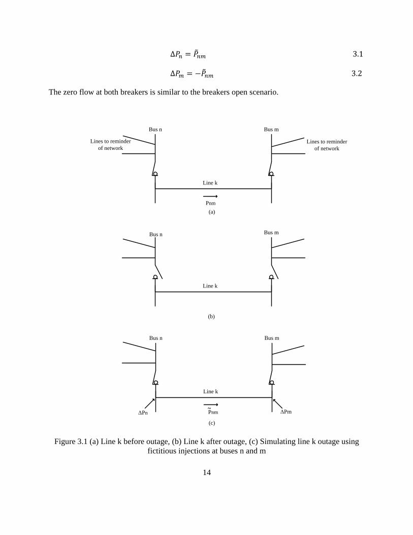
3.3 Nodal injections in a Simplified System Model
The theory behind the proposed scheme is introduced in this section using a simple 2-bus
system. The system consists of a double-line circuit connecting buses i and j as shown in figure
3.2. It is assumed that the lines are represented using an equivalent model. The nodal states of
the buses, Vi∠δi and Vj∠δj, as well as the flows of the two lines are monitored using PMUs.
The power flow equations at bus i can be expressed as follows:
𝑃𝑖 = ∑ (∑[𝑉𝑖2 − 𝑉𝑖𝑉𝑗 cos(𝛿𝑖 − 𝛿𝑗)]. 𝑔𝐿 − 𝑉𝑖𝑉𝑗 sin(𝛿𝑖 − 𝛿𝑗) . 𝑏𝐿
𝑀
𝐿=1
)
𝑁−1
𝑗=1
3.3
𝑄𝑖 =∑(∑−𝑉𝑖2. 𝑏𝐿_𝑠ℎ + [𝑉𝑖
2 − 𝑉𝑖𝑉𝑗cos (𝛿𝑖 − 𝛿𝑗)]. 𝑏𝐿 − 𝑉𝑖𝑉𝑗 sin(𝛿𝑖 − 𝛿𝑗) . 𝑔𝐿
𝑀
𝐿=1
)
𝑁
𝑗=1
3.4
Where:
Pi ≡ Injected active power at bus i
Qi ≡ Injected reactive power at bus i
N ≡ Number of buses in the system
M ≡ Number of lines connecting buses i and j
gL ≡ Series conductance of line L
bL ≡ Series susceptance of line L
bL_sh ≡ Shunt charging susceptance of line L
In this system, N=2 and M=2. When substituting the nodal states of the system during
normal operating conditions i.e. with both lines in service, the resulting Pi and Qi are equal to the

16
net load and generation at the bus. However, if an outage occurs on one of the circuits, the nodal
states will change. Appling these states to the aforementioned power flow equations while
keeping the original system model i.e. both lines are included, would result in a total injected
power Pi and Qi which differ from the net load and generation at the bus. These injection errors
represent the fictitious injections Pi−inj and Qi−inj that simulate an outage.
𝑃𝑖−𝑖𝑛𝑗 = 𝑃𝑖 − (𝑃𝑖𝑔 − 𝑃𝑖𝑑) 3.5
𝑄𝑖−𝑖𝑛𝑗 = 𝑄𝑖 − (𝑄𝑖𝑔 − 𝑄𝑖𝑑) 3.6
Similarly, when applying the power flow equations to bus j, approximately the same
amount of active injected power will appear with a negative sign to drive the flow through the
breakers of the outraged line to zero. The difference will be caused by the 𝑖2𝑅 losses in the i-j
branch.
Pj−inj ≈ −Pi−inj 3.7
The case is not necessarily the same for reactive power since under light load conditions,
the outaged line might generate sufficient vars to mask this power circulation effect, and
conversely absorb excessive vars under heavy load conditions.
17
(a)
Figure 3.2 (a) Two-Bus system with both lines in service, (b) One of the lines out of service, (c)
outaged line in service with power injections
Vi∠δi
i1
Vj∠δj
i1
(b)
iinj i2=0
Pi-inj
Qi-inj
Vi∠δi
i1
Vj∠δj
i1
Pj-inj
Qj-inj
(c)
Vi∠δi
i1 i1
Vj∠δj
i1
i2 i1
i2 i1
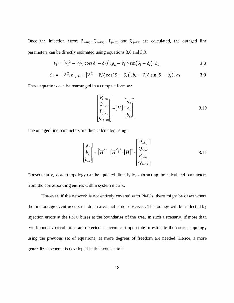
18
Once the injection errors Pi−inj , Qi−inj , Pj−inj and Qj−inj are calculated, the outaged line
parameters can be directly estimated using equations 3.8 and 3.9.
𝑃𝑖 = [𝑉𝑖2 − 𝑉𝑖𝑉𝑗 cos(𝛿𝑖 − 𝛿𝑗)]. 𝑔𝐿 − 𝑉𝑖𝑉𝑗 sin(𝛿𝑖 − 𝛿𝑗) . 𝑏𝐿 3.8
𝑄𝑖 = −𝑉𝑖2. 𝑏𝐿_𝑠ℎ + [𝑉𝑖
2 − 𝑉𝑖𝑉𝑗cos (𝛿𝑖 − 𝛿𝑗)]. 𝑏𝐿 − 𝑉𝑖𝑉𝑗 sin(𝛿𝑖 − 𝛿𝑗) . 𝑔𝐿 3.9
These equations can be rearranged in a compact form as:
Sh
L
L
injj
injj
inji
inji
b
b
g
H
Q
P
Q
P
3.10
The outaged line parameters are then calculated using:
injj
injj
inji
inji
TT
Sh
L
L
Q
P
Q
P
HHH
b
b
g1
3.11
Consequently, system topology can be updated directly by subtracting the calculated parameters
from the corresponding entries within system matrix.
However, if the network is not entirely covered with PMUs, there might be cases where
the line outage event occurs inside an area that is not observed. This outage will be reflected by
injection errors at the PMU buses at the boundaries of the area. In such a scenario, if more than
two boundary circulations are detected, it becomes impossible to estimate the correct topology
using the previous set of equations, as more degrees of freedom are needed. Hence, a more
generalized scheme is developed in the next section.

19
3.4 Complete Algorithm
The scheme developed in this thesis assumes only n-1 contingency at any given time.
This scheme continuously applies system states obtained from PMUs to the present system
topology (equations 3.3, 3.4). In case of a line outage event, a set of injections that is not
accounted for appears (equations 3.5, 3.6). However, to account for the stochastic nature of
errors in PMU measurements, a threshold value, below which the injection errors are ignored, is
defined. This threshold could be a percentage of the total system load for instance.
The identification of the outaged line is relatively easy if all system buses are monitored
using PMUs. In such a scenario, a pair of injection errors is detected at the outaged line ends
when applying system states to the complete system model. After identifying these two buses,
the algorithm constructs the event area model which consists of the two buses along with all lines
connected between them, their generation and load as well as the power transferred between each
bus and the remainder of the system. These power flows are then treated as load or generation
depending on their direction.
Once the event area model is constructed, a trial-and-error method is adopted to detect
the outaged line. This is essentially done by first excluding the suspected line from event area
model, reducing this model to eliminate unobserved buses and then applying current system
states to this updated topology to calculate the new injection errors. If the resulting errors are
below the pre-defined threshold, the suspected line is recognized to be out and the present system
topology is updated accordingly. Otherwise, the next candidate line is considered.
The algorithm could be further applied to reduced systems where parts of the network are
not covered by PMU measurements. In this situation, it would be impossible to estimate the

20
states for unobserved buses unless the exact topology is known. Conversely, these states are
needed to determine the exact topology of the system.
At first, a reduced model of the system consisting only of observed buses is constructed.
The unobserved nodes are typically tie-buses with no loading. Line outage events in an
unobserved portion of the system will cause injection errors at the boundaries of the unobserved
area in the reduced network. These boundaries are defined by PMU buses which surrounds the
unobserved area. The scheme can make advantage of such behavior to circle the area that
contains the event. Strictly speaking, the scheme only considers the cases in which injection
errors appear in more than one bus. In addition, these buses must be either directly connected or
form boundaries for a specific unobserved area. The detection of injection error in a single bus
could represent an unaccounted for load or simply a too high a value of the threshold level. On
the other hand, detection of injections in two different areas could represent a previous outage
that was not taken into account in the present system topology.
3.4.1 Determining the Event Area
To detect the outaged line in a specific event area, all the buses in this area, which
consists of the unobserved buses with their PMU boundaries, must be identified first. The
algorithm essentially starts from an observed bus with significant injection error and attempts to
find all buses connected to it which also experience notable errors. It is to be noted that two
observed buses with injection errors could either be directly connected to each other or a series
of unobserved buses might exist between them. The following steps are used to determine the
event area buses:
1. Define empty matrices:

21
AREA, TEMP, PATH.
2. For each bus in the system:
Check if the injection error is greater than the pre-defined threshold. If yes, add the
bus to AREA matrix and go to step 3. Otherwise, check the next bus.
3. For all lines connected to the bus:
If the remote terminal bus is observed and its injection error is greater than the
threshold, add it to AREA and move on to the next line. Else if the remote terminal
bus is unobserved, add it to TEMP matrix, add both terminal buses to the first row of
PATH and go to step 5. Otherwise, check the next line.
4. Go to the next bus in 2.
5. While TEMP is not empty
a. Create new empty matrices TEMP1 and PATH1. Set New-Path-Pointer to 1
and set Current-Path-Pointer to 1.
b. For all unobserved buses in TEMP:
i. Store the row of the PATH matrix which is pointed to by Current-
Path-Pointer in a new matrix called Current-Path.
ii. For all lines connected to the unobserved bus, if the remote terminal
bus is not a part of Current-Path and is observed and its injection
error is greater than the threshold, add the remote terminal bus and
Current-Path to AREA and move to the next line. Else if the remote
terminal bus is unobserved and not included in Current-Path, add this
remote bus to TEMP1, enter both Current-Path and the remote bus in

22
Path1 in the row which is pointed to by New-Path-Pointer, increase
New-Path-Pointer by one and move on to the next line. Otherwise,
go to the next line.
c. Increase Current-Path-Pointer by 1 and go to the next unobserved bus in 5.b.
d. TEMP=TEMP1
Path=Path1
6. Go to the next line in 3
The following example is used to demonstrate these steps. Figure 3.3 shows a model of a
simple 7-bus system. Buses 1, 4, 5, 6 and 7 are observed using PMUs. It is assumed that line 2-3
experienced an outage which will be reflected as injection errors at buses 1, 4 and 5.
1 7
5
GU1
L3
26 3 4
GU2
L2L1
Figure 3.3 7-bus system
Starting from bus 1, the algorithm proceeds as follows:
1. AREA = [ ]; TEMP = [ ]; PATH = [ ];

23
2. For bus 1:
Since injection error at this bus is greater than threshold value, this bus will be
included in the area.
AREA = [1];
3. For Line 1-2:
Since the remote terminal bus (bus 2) is unobserved, TEMP and PATH will be
updated as follows:
TEMP = [2]
PATH = [1 2]
The algorithm then jumps to step 5.
5. While TEMP is not empty:
a. TEMP1 = [ ]; PATH1 = [ ];
New-Path-Pointer = 1; Current-Path-Pointer = 1;
b. For Bus 2 in TEMP
i. Current-Path = [1 2]
ii. For Line 1-2
No action is needed because terminal bus (bus 1) is included in Current-
Path
For Line 2-3
Since Bus 3 is unobserved:
TEMP1 = [3]
PATH1 = [1 2 3]

24
New-Path-Pointer = 2
For Line 2-5
Since Bus 5 is observed with injection error, bus 5 and Current-Path will
be included in the area:
AREA = [1 2 5]
c. Current-Path-Pointer = 2
d. TEMP = [3]
PATH = [1 2 3]
Since TEMP is not empty, step 5 is repeated again with the new values for TEMP
and PATH:
5. a. TEMP1 = [ ]; PATH1 = [ ];
New-Path-Pointer = 1; Current-Path-Pointer = 1;
b. For Bus 3 in TEMP
i. Current-Path = [1 2 3]
ii. For Line 3-2
No action is needed because terminal bus (bus 2) is included in Current-Path
For Line 3-4
Since Bus 4 is observed with injection error, bus 4 and Current-Path will
be included in the area:
AREA = [1 2 5 3 4]
c. Current-Path-Pointer = 2
d. TEMP = [ ]; PATH = [ ]

25
Since TEMP matrix is empty, the while loop condition is not satisfied anymore.
Hence, the algorithm will proceed to the next line (Step 3)
3. For Line 1-6
The terminal bus (bus 6) is observed but it has no injection error. Hence, no action
is taken for this line.
The algorithm moves to the next observed bus with injection error and the same steps are
repeated until all observed buses are checked.
The AREA resulting from this process consists of buses 1, 2, 3, 4 and 5 which represent the
event area.
3.4.2 Identifying the Outaged Element
Once all buses contained within the event area are specified, a model is constructed using
these buses along with their connectivity data. The power transferred between each PMU bus
and the rest of the system together with the generation and load connected to each bus are also
considered in this model. The injection errors at each observed bus are then calculated using
equations (3.12, 3.13).
𝑃𝑖−𝑖𝑛𝑗 = 𝑃𝑖 −
(
𝑃𝑖𝑔 − 𝑃𝑖𝑑 − ∑ 𝑃𝑖𝑗
𝑁
𝑗=1𝑗∉𝑒𝑣𝑒𝑛𝑡 𝑎𝑟𝑒𝑎 )
3.12
𝑄𝑖−𝑖𝑛𝑗 = 𝑄𝑖 −
(
𝑄𝑖𝑔 − 𝑄𝑖𝑑 − ∑ 𝑄𝑖𝑗
𝑁
𝑗=1𝑗∉𝑒𝑣𝑒𝑛𝑡 𝑎𝑟𝑒𝑎 )
3.13

26
Afterwards, the algorithm follows the same trial-and-error method described earlier in order to
identify the outaged line. This method starts by eliminating the suspected line from the topology.
Matrix partitioning is then applied to determine the equivalent admittances between the observed
buses. The updated topology is examined against the current states of these buses to calculate the
new injection errors at the boundaries. Once the errors are eliminated, the outage line is
recognized and the overall system topology is updated. It is to be stated that an improved search
criterion could be implemented to enhance the search time. This criterion assumes that the
outaged line is close to buses with higher injection errors. Hence, the search is started with lines
connected to these buses.
It must be noted that the injection errors at some boundaries of the area might sometimes
be less than the threshold. This situation will introduce difficulties in defining the search area. To
mitigate this issue, the algorithm uses the unobserved buses found after applying the previous
steps along with the connectivity data to determine the remaining boundaries and unobserved
buses of the area. A similar procedure to that described in step 5 is adopted to achieve this
purpose.
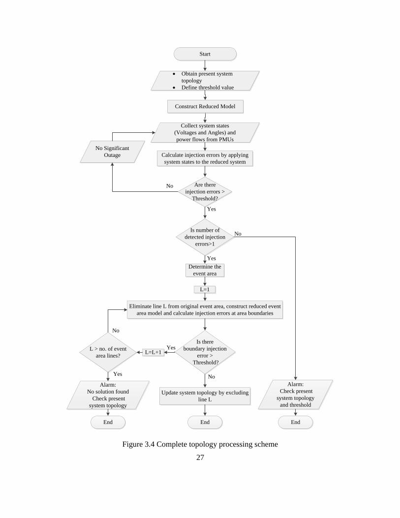
The overall topology processing scheme developed in this work is summarized in the
flowchart shown in figure 3.3.
27
Start
Collect system states
(Voltages and Angles) and
power flows from PMUs
Calculate injection errors by applying
system states to the reduced system
Are there
injection errors >
Threshold?
No Significant
Outage
Is number of
detected injection
errors>1
Alarm:
Check present
system topology
and threshold
Determine the
event area
L=1
Eliminate line L from original event area, construct reduced event
area model and calculate injection errors at area boundaries
Is there
boundary injection
error >
Threshold?
L=L+1L > no. of event
area lines?
Alarm:
No solution found
Check present
system topology
Update system topology by excluding
line L
End
Yes
Yes
No
No
No
Yes
No
Yes
Obtain present system
topology
Define threshold value
End End
Construct Reduced Model
Figure 3.4 Complete topology processing scheme

28
CHAPTER 4
4 RESULTS AND DISCUSSION
4.1 Test System Description
The algorithm was tested on the IEEE39-bus system, commonly known as 10-machine
New-England power system. This system consists of 10 generators, 18 Loads, 12 transformers
and 34 transmission lines as shown in figure 4.1. Complete system data are tabulated in
Appendix A. Generator 1 which represents the aggregation of a large number of generators is set
to be the swing unit. It is assumed that all generator and load buses are observed using PMUs.
The remaining 12 buses are unobserved.

29
Figure 4.1 IEEE39-bus system
4.2 Simulation Results
4.2.1 Normal Operating Condition
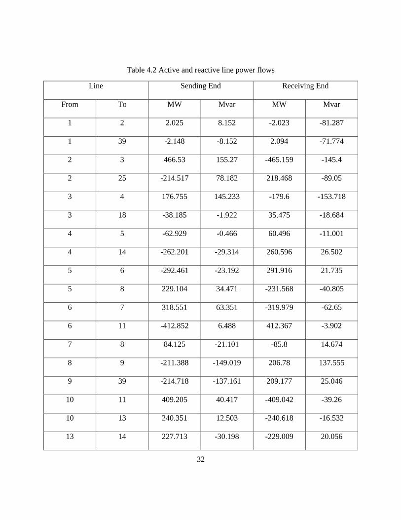
The following tables list the load flow results of the system prior to the application of any
outage. Table 4.1 shows system states at each bus whereas table 4.2 lists active and reactive
power flow on each line.

30
Table 4.1 System states during normal operating conditions
Bus Voltage magnitude
(pu)
Angle
(degrees)
1 1.038 -0.045
2 1.02 -0.005
3 0.991 -3.879
4 0.956 -6.053
5 0.956 -5.556
6 0.957 -5.082
7 0.949 -6.912
8 0.949 -7.165
9 1.008 -2.839
10 0.963 -1.887
11 0.959 -2.969
12 0.94 -2.805
13 0.961 -2.524
14 0.962 -3.966
15 0.969 -3.551
16 0.988 -1.647
17 0.992 -2.658
18 0.99 -3.588
19 0.99 4.158

31
20 0.987 3.172
21 0.995 0.926
22 1.021 5.634
23 1.02 5.407
24 0.996 -1.522
25 1.027 1.333
26 1.017 -0.328
27 0.999 -2.634
28 1.019 3.398
29 1.02 6.316
30 1.048 2.423
31 0.982 -2.032
32 0.983 6.007
33 0.997 9.355
34 1.012 8.351
35 1.049 10.609
36 1.063 13.425
37 1.028 8.14
38 1.027 13.396
39 1.03 0
32
Table 4.2 Active and reactive line power flows
Line Sending End Receiving End
From To MW Mvar MW Mvar
1 2 2.025 8.152 -2.023 -81.287
1 39 -2.148 -8.152 2.094 -71.774
2 3 466.53 155.27 -465.159 -145.4
2 25 -214.517 78.182 218.468 -89.05
3 4 176.755 145.233 -179.6 -153.718
3 18 -38.185 -1.922 35.475 -18.684
4 5 -62.929 -0.466 60.496 -11.001
4 14 -262.201 -29.314 260.596 26.502
5 6 -292.461 -23.192 291.916 21.735
5 8 229.104 34.471 -231.568 -40.805
6 7 318.551 63.351 -319.979 -62.65
6 11 -412.852 6.488 412.367 -3.902
7 8 84.125 -21.101 -85.8 14.674
8 9 -211.388 -149.019 206.78 137.555
9 39 -214.718 -137.161 209.177 25.046
10 11 409.205 40.417 -409.042 -39.26
10 13 240.351 12.503 -240.618 -16.532
13 14 227.713 -30.198 -229.009 20.056

33
14 15 -35.91 -46.258 31.489 12.916
15 16 -354.606 -165.722 354.571 164.434
16 17 189.551 -63.944 -190.257 54.417
16 19 -503.285 43.642 508.779 -22.09
16 21 -329.042 -36.469 329.623 26.429
16 24 -43.41 -139.888 43.103 134.443
17 18 194.454 1.48 -195.592 -11.183
17 27 -6.876 -55.773 3.958 24.317
21 22 -602.805 -141.416 608.904 169.395
22 23 45.592 1.775 -41.897 -20.468
23 24 358.163 49.729 -352.833 -42.213
25 26 97.491 -1.991 -96.236 -48.545
26 27 287.548 88.62 -287.53 -99.699
26 28 -141.244 -26.785 146.404 -44.576
26 29 -190.585 -30.282 203.707 -53.046
28 29 -346.085 17.351 352.091 -25.11
A reduced system model (27-bus system) was derived after eliminating the unobserved
nodes (1, 2, 5, 6, 9, 10, 11, 13, 14, 17, 19 and 22). Table 4.3 shows the difference between
calculated and observed power injections when applying system states of PMU buses (Table 4.1)
to this reduced model (equation 3.5, 3.6). Setting the threshold value to 1% of total system load,

34
the amount of these injection errors is negligible which reflects the present normal operating
conditions. The minor values shown are due to calculation rounding.
Table 4.3 Active and reactive power injection errors during normal operating conditions
Observed bus Active power injection errors
(pu)
Reactive power injection errors
(pu)
3 0.0509 0.0022
4 -0.0009 0.0000
7 -0.0025 0.0000
8 -0.0059 0.0000
12 0.0012 0.0000
15 -0.0023 0.0000
16 -0.0007 0.0000
18 -0.0005 0.0000
20 0.0004 0.0000
21 -0.0009 0.0000
23 -0.0019 0.0000
24 0.0000 -0.0000
25 -0.1400 0.0141
26 0.0000 -0.0000
27 0.0003 0.0000
28 -0.0000 -0.0000

35
29 -0.0000 -0.0000
30 0.0670 0.0098
31 0.0024 0.0000
32 0.0047 0.0001
33 0.0005 -0.0000
34 0.0000 -0.0000
35 0.0030 0.0001
36 0.0000 -0.0000
37 0.0000 -0.0000
38 -0.0000 -0.0000
39 0.0274 0.0002
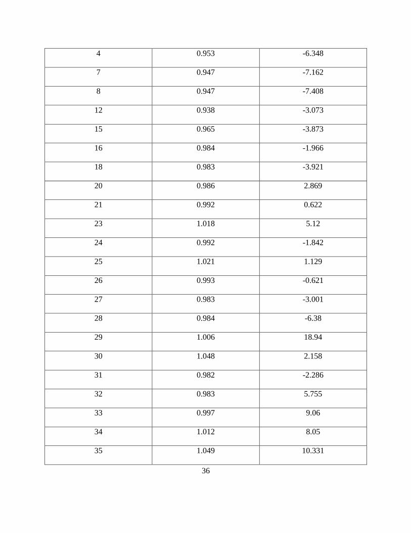
4.2.2 Line Outage between Two Observed Buses
In this section, the algorithm was tested when a line outage event between buses 28 and
29 occurred. System states of PMU buses during this event are shown in table 4.4. Applying
these states to the reduced 27-bus system topology with line 28-29 in-service resulted in active
and reactive power injection errors shown in table 4.5.
Table 4.4 System states during outage of line 28-29
Bus Voltage magnitude
(pu)
Angle
(degrees)
3 0.986 -4.192
36
4 0.953 -6.348
7 0.947 -7.162
8 0.947 -7.408
12 0.938 -3.073
15 0.965 -3.873
16 0.984 -1.966
18 0.983 -3.921
20 0.986 2.869
21 0.992 0.622
23 1.018 5.12
24 0.992 -1.842
25 1.021 1.129
26 0.993 -0.621
27 0.983 -3.001
28 0.984 -6.38
29 1.006 18.94
30 1.048 2.158
31 0.982 -2.286
32 0.983 5.755
33 0.997 9.06
34 1.012 8.05
35 1.049 10.331

37
36 1.063 13.15
37 1.028 7.971
38 1.027 26.079
39 1.03 0
Table 4.5 Active and reactive power injection errors during outage of line 28-29
Observed bus Active power injection errors
(pu)
Reactive power injection errors
(pu)
3 0.0504 0.0022
4 -0.0009 0.0000
7 -0.0025 0.0000
8 -0.0059 0.0000
12 0.0012 0.0000
15 -0.0023 0.0000
16 -0.0007 0.0000
18 -0.0005 0.0000
20 0.0004 0.0000
21 -0.0009 0.0000
23 -0.0019 0.0000
24 -0.0000 -0.0000
25 -0.1381 0.0139
26 0.0000 -0.0000

38
27 0.0003 0.0000
28 27.3558 -7.2888
29 -28.5168 -4.9870
30 0.0670 0.0098
31 0.0024 0.0000
32 0.0047 0.0001
33 0.0005 -0.0000
34 0.0000 -0.0000
35 0.0030 0.0000
36 0.0000 -0.0000
37 0.0000 -0.0000
38 0.0000 -0.0001
39 0.0274 0.0002
Taking into account that the threshold value is defined as 0.6 pu for active power
injection errors and 0.14 pu for reactive errors, the algorithm detected only the injection errors at
buses 28 and 29. Since there is a single line connected between these two buses, this line was
recognized to be out. The total processing time for this case was less than 0.03 seconds. After
updating system topology, the errors ceased to exist as shown in table 4.6.
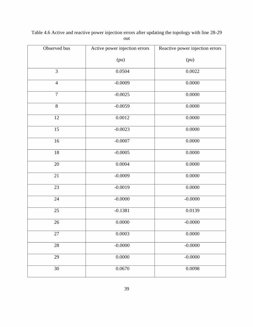
39
Table 4.6 Active and reactive power injection errors after updating the topology with line 28-29
out
Observed bus Active power injection errors
(pu)
Reactive power injection errors
(pu)
3 0.0504 0.0022
4 -0.0009 0.0000
7 -0.0025 0.0000
8 -0.0059 0.0000
12 0.0012 0.0000
15 -0.0023 0.0000
16 -0.0007 0.0000
18 -0.0005 0.0000
20 0.0004 0.0000
21 -0.0009 0.0000
23 -0.0019 0.0000
24 -0.0000 -0.0000
25 -0.1381 0.0139
26 0.0000 -0.0000
27 0.0003 0.0000
28 -0.0000 -0.0000
29 0.0000 -0.0000
30 0.0670 0.0098

40
31 0.0024 0.0000
32 0.0047 0.0001
33 0.0005 -0.0000
34 0.0000 -0.0000
35 0.0030 0.0000
36 0.0000 -0.0000
37 0.0000 -0.0000
38 0.0000 -0.0001
39 0.0274 0.0002
4.2.3 Outage Events in Unobserved Area
4.2.3.1 Line Outage - Case Study A
It can be seen from figure 4.1 that the unobserved bus 22 is connected to three PMU
buses, 21, 23 and 35. An outage event between buses 21 and 22 will change the states of the
system. Applying these states to the original 27-bus system resulted in power injection errors at
the boundaries of the area (buses 21, 23 and 35) as shown in table 4.7.
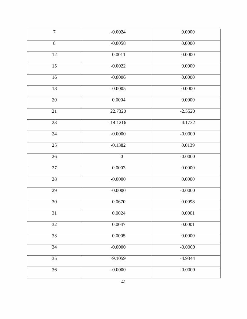
Table 4.7 Active and reactive power injection errors during outage of line 21-22
Observed bus Active power injection errors
(pu)
Reactive power injection errors
(pu)
3 0.0493 0.0021
4 -0.0009 0.0000
41
7 -0.0024 0.0000
8 -0.0058 0.0000
12 0.0011 0.0000
15 -0.0022 0.0000
16 -0.0006 0.0000
18 -0.0005 0.0000
20 0.0004 0.0000
21 22.7320 -2.5520
23 -14.1216 -4.1732
24 -0.0000 -0.0000
25 -0.1382 0.0139
26 0 -0.0000
27 0.0003 0.0000
28 -0.0000 0.0000
29 -0.0000 -0.0000
30 0.0670 0.0098
31 0.0024 0.0001
32 0.0047 0.0001
33 0.0005 0.0000
34 -0.0000 -0.0000
35 -9.1059 -4.9344
36 -0.0000 -0.0000

42
37 -0.0000 -0.0000
38 -0.0000 -0.0000
39 0.0274 0.0002
Once the event area buses are identified, the algorithm retrieves the data of the lines and
transformers belonging to the area. In the subsequent processing, the algorithm deals only with
this area while considering the power transferred between its boundaries and the rest of the
system as load or generation depending on its direction. These flows are shown in table 4.8. The
algorithm then starts the trial-and-error process to identify the line that will cause injection errors
to disappear. This condition is satisfied when line 21-22 is removed from the configuration
(Table 4.9). It worth mentioning that the algorithm computational time for this case was also less
than 0.03 sec.
Table 4.8 Power transferred between event area boundaries and the rest of the system during line
21-22 outage event
Line Power
From To MW Mvar
21 16 -275.681 -114.872
23 24 970.11 237.964
23 36 -558.303 -172.91

43
Table 4.9 Active and reactive power injection errors when updating the topology with line 21-22
out
Observed bus Active power injection errors
(pu)
Reactive power injection errors
(pu)
21 0.0168 -0.0000
23 -0.1206 0.0000
35 0.0015 0.0000
4.2.3.2 Line Outage - Case Study B
Referring to figure 4.1, it can be noted that PMU buses 4, 7, 8, 12, 15, 31 and 32 form the
boundaries of an unobserved area which contains 11 lines and 3 transformers. The outage of any
of these components will be reflected as injection errors at the boundaries of the area.
Considering the scenario in which line 10-11 is out, the injection errors experienced when
applying system states to the 27-bus system are shown in table 4.10. Although the injection
errors at buses 4 and 12 were below the threshold, the algorithm was still able to include these
buses in the area boundaries as they are connected to unobserved buses which are already
included in the event area.
Table 4.10 Active and reactive power injection errors during outage of line 10-11
Observed bus Active power injection errors
(pu)
Reactive power injection errors
(pu)
3 0.0505 0.0022
4 -0.5105 0.0722

44
7 2.0945 -0.1966
8 1.1934 -0.1264
12 0.3678 0.0689
15 -0.9549 0.0277
16 -0.0007 0.0000
18 -0.0005 0.0000
20 0.0004 0.0000
21 -0.0009 0.0000
23 -0.0019 0.0000
24 -0.0000 -0.0000
25 -0.1398 0.0141
26 0.0000 -0.0000
27 0.0003 0.0000
28 -0.0000 -0.0000
29 -0.0000 -0.0000
30 0.0670 0.0098
31 0.8123 0.0437
32 -3.0233 -0.9321
33 0.0005 -0.0000
34 0.0000 -0.0000
35 0.0030 0.0000
36 0.0000 -0.0000

45
37 0.0000 -0.0000
38 0.0000 -0.0000
39 0.0274 0.0002
As explained earlier, the algorithm then constructs the event area model and begins the
trial-and-error process to find the outaged line. Table 4.11 shows the resulting injection errors at
the boundaries of the area during this iterative process. The errors disappeared only when line
10-11 is considered out. The total processing time was again below 0.03 seconds.
Table 4.11 Active power injection errors during trial-and-error process for case B
Candidate
line
Boundary
4-5 4-14 5-6 5-8 6-7 6-11 7-8 10-11
4 0.252 -3.653 -1.668 0.944 1.009 -0.650 -0.493 0.017
7 1.849 2.348 3.593 3.297 -2.798 -0.544 2.555 0.001
8 0.938 1.3905 -0.247 -2.318 2.694 -0.262 0.786 0.047
12 0.325 0.911 0.630 0.578 0.807 2.675 0.368 0.001
15 -0.964 0.643 -0.868 -0.885 -0.812 -0.232 -0.951 0.001
31 0.720 0.910 1.384 1.269 1.768 -0.215 0.812 0.002
32 -3.064 -2.492 -2.768 -2.820 -2.602 -0.686 -3.023 0.003

46
4.2.3.2 Transformer Outage- Case Study C
This study considers the outage event of transformer T12 which is connected between
buses 12 and 13. Referring to figure 4.1, it can be seen that T12 belongs to the same area as in
Case B. The resulting injection errors during this event are listed in table 4.12. Based on the
predefined threshold value, only three reactive power injection errors were detected on buses 4,
12 and 32. Yet, the algorithm was still able to define the area boundaries as illustrated earlier.
The scheme then proceeded normally to identify the outaged element in less than 0.03 seconds.
Table 4.12 Active and reactive power injection errors during outage of transformer T12
Observed bus Active power injection errors
(pu)
Reactive power injection errors
(pu)
3 0.0509 0.0022
4 -0.0882 -0.2696
7 -0.0383 -0.0957
8 -0.0271 -0.0545
12 0.2017 0.7771
15 -0.0414 -0.1340
16 -0.0007 0.0000
18 -0.0005 0.0000
20 0.0004 0.0000
21 -0.0009 0.0000
23 -0.0019 0.0000

47
24 0.0000 -0.0000
25 -0.1400 0.0141
26 0.0000 -0.0000
27 0.0003 0.0000
28 -0.0000 -0.0000
29 -0.0000 -0.0000
30 0.0670 0.0098
31 -0.0057 -0.0382
32 -0.0044 -0.2261
33 0.0005 -0.0000
34 0.0000 -0.0000
35 0.0030 0.0001
36 0.0000 -0.0000
37 0.0000 -0.0000
38 0.0000 -0.0000
39 0.0274 0.0002
4.2.4 Other Outage Events
Using the threshold values defined earlier, the algorithm was able to detect and identify
all line outage events except one in the IEEE39-bus system in less than 2 cycles. This undetected
event was the outage of line 1-39. During this outage, fictitious reactive power injection was

48
detected on bus 39 only whereas active power injection errors were insignificant at all buses.
Hence, the algorithm alarmed the user to check the threshold value as well as system topology.
It can be noted that the preoutage power flow on this line was minor compared to other
lines in the system (Table 4.2) which justifies the low injection error values. This indicates that
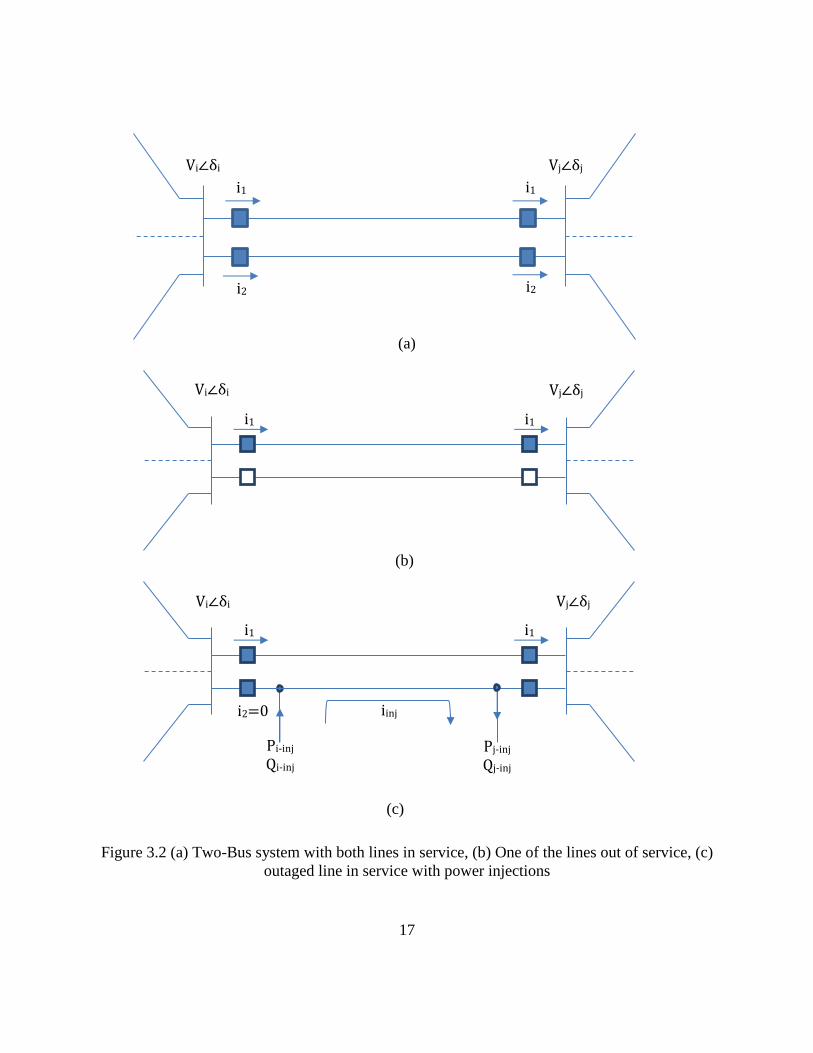
the line has insignificant effect on system stability. To verify this conclusion, the effect of the
line on voltage stability of the system was measured using the P-index. This index is a voltage
stability indicator that is based on normalized voltage and power sensitivities [11].
According to this index, bus-12 of the IEEE39-bus system is the weakest bus. Figure 4.2
shows the P-index for this bus during normal operating conditions and during the outage event of
line 1-39. The P-index of bus-12 during the outage of line 21-22, which causes relatively high
injections, is also shown in the figure (section 4.2.2).
Figure 4.2 Bus-12 P-index during different operating conditions
0 0.5 1 1.5 2 2.50
0.2
0.4
0.6
0.8
1
Active Power Loading (pu)
Bus V
oltage (
pu)
Bus 12 during normal operating conditions
Bus 12 during line 1-39 outage
Bus 12 during line 21-22 outage

49
It can be seen from this figure that the P-index of bus-12 was slightly affected by the outage of
line 1-39 whereas the outage event of line 21-22 severely affected it.

50
CHAPTER 5
5 CONCLUSION
5.1 Conclusion
In this work, a fast and simple yet reliable topology processing scheme was developed.
This scheme is based on PMU measurements. However, it can be applied on reduced systems in
which network buses are not entirely covered with PMUs. The introduced algorithm
continuously applies system states (voltages and angles) to the present system model in order to
calculate injections at the observed buses. In case of an outage, unaccounted for injections appear
in the outage location. If the outaged component was connected between two observed buses,
injection errors appear only at these buses. However, if the outage event occurred in unobserved
area, it will be reflected as injection errors at the boundaries of this area. Once errors are
detected, the algorithm determines all the candidate equipment within the event area and follows
a trial-and-error method to find the element that eliminates these injection errors.
The performance of the scheme was tested using the IEEE39-bus system where PMUs
were deployed only at load and generation buses. The algorithm was successfully able to detect
and identify various outage events in less than 2 cycles. This short processing time is due to the
simple detection procedure which does not include any processing of breaker status information.
In addition, the algorithm limits the area to be searched to a minimal subset of the original
network which leads to further improvement in the overall processing time.

51
5.2 Future Work
As a future work, the algorithm can be improved to account for changes in transformer
tap positions. Moreover, an optimization technique can be implemented instead of the trial-and-
error method adopted in this work. This might enhance the search time in cases where the event
area is relatively large.

52
REFERENCES
[1] A. J. Wood and B. F. Wollenberg, Power generation, operation, and control. John Wiley
& Sons, 2012.
[2] A. M. Sasson, S. T. Ehrmann, P. Lynch, and L. S. V. Slyck, "Automatic Power System
Network Topology Determination," IEEE Transactions on Power Apparatus and
Systems, vol. PAS-92, no. 2, pp. 610-618, 1973.
[3] A. Bose and K. A. Clements, "Real-time modeling of power networks," Proceedings of
the IEEE, vol. 75, no. 12, pp. 1607-1622, 1987.
[4] M. Farrokhabadi, "Automated topology processing for conventional, phasor-assisted and
phasor-only state estimators," Master’s thesis, Royal Institute of Technology (KTH),
2012.
[5] M. Prais and A. Bose, "A topology processor that tracks network modifications," IEEE
Transactions on Power Systems, vol. 3, no. 3, pp. 992-998, 1988.
[6] M. V. Mynam, A. Harikrishna, and V. Singh, "Synchrophasors redefining SCADA
systems," Schweitzer Engineering Laboratories, Inc, 2013.
[7] M. Salah Aldeen Mohamed Zeyada, "Adaptive underfrequency load shedding based on
real time simulation," Master’s thesis, University of Tennessee at Chattanooga (UTC),
2014.
[8] Z. Dong and P. Zhang, Emerging techniques in power system analysis. Springer, 2010.
[9] J. E. Tate and T. J. Overbye, "Line Outage Detection Using Phasor Angle
Measurements," IEEE Transactions on Power Systems, vol. 23, no. 4, pp. 1644-1652,
2008.
[10] H. Sehwail and I. Dobson, "Locating line outages in a specific area of a power system
with synchrophasors," in North American Power Symposium (NAPS), 2012, 2012, pp. 1-
6.
[11] M. Kamel, "Development and Application of a New Voltage Stability Index for On-Line
Monitoring and Shedding," Master’s thesis, University of Tennessee at Chattanooga
(UTC), 2016.

53
APPENDIX A
IEEE39-BUS SYSTEM DATA

54
The following tables provide the data of the IEEE39-bus system on a 100 MVA base.
Table A.1: steady state data for load and generation for load flow purposes
Bus No. Bus Type Voltage
(PU)
Load
(MW)
Load
(MVAR)
Generation
(MW)
1 P-Q - 0 0 0
2 P-Q - 0 0 0
3 P-Q - 322 2.4 0
4 P-Q - 500 184 0
5 P-Q - 0 0 0
6 P-Q - 0 0 0
7 P-Q - 233.8 84 0
8 P-Q - 522 176 0
9 P-Q - 0 0 0
10 P-Q - 0 0 0
11 P-Q - 0 0 0
12 P-Q - 7.5 88 0
13 P-Q - 0 0 0
14 P-Q - 0 0 0
15 P-Q - 320 153 0
16 P-Q - 329 32.3 0
17 P-Q - 0 0 0

55
18 P-Q - 158 30 0
19 P-Q - 0 0 0
20 P-Q - 628 103 0
21 P-Q - 274 115 0
22 P-Q - 0 0 0
23 P-Q - 247.5 84.6 0
24 P-Q - 308.6 -92.2 0
25 P-Q - 224 47.2 0
26 P-Q - 139 17 0
27 P-Q - 281 75.5 0
28 P-Q - 206 27.6 0
29 P-Q - 283.5 26.9 0
30 P-V 1.0475 0 0 250
31 P-V 0.982 0 0 200
32 P-V 0.9831 0 0 650
33 P-V 0.9972 0 0 632
34 P-V 1.0123 0 0 508
35 P-V 1.0493 0 0 650
36 P-V 1.0635 0 0 560
37 P-V 1.0278 0 0 540
38 P-V 1.0265 0 0 830
39 V-𝛿 1.03 1104 250 1000

56
Table A.2: Transmission lines and transformers data
From Bus To Bus R (pu) X (pu) B(pu)
1 2 0.0035 0.0411 0.6987
1 39 0.001 0.025 0.7500
2 3 0.0013 0.0151 0.2572
2 25 0.007 0.0086 0.1460
3 4 0.0013 0.0213 0.2214
3 18 0.0011 0.0133 0.2138
4 5 0.0008 0.0128 0.1342
4 14 0.0008 0.0129 0.1382
5 6 0.0002 0.0026 0.0434
5 8 0.0008 0.0112 0.1476
6 7 0.0006 0.0092 0.1130
6 11 0.0007 0.0082 0.1389
7 8 0.0004 0.0046 0.0780
8 9 0.0023 0.0363 0.3804
9 39 0.001 0.025 1.2000
10 11 0.0004 0.0043 0.0729
10 13 0.0004 0.0043 0.0729
13 14 0.0009 0.0101 0.1732
14 15 0.0018 0.0217 0.3660

57
15 16 0.0009 0.0094 0.1710
16 17 0.0007 0.0089 0.1342
16 19 0.0016 0.0195 0.3040
16 21 0.0008 0.0135 0.2548
16 24 0.0003 0.0059 0.0680
17 18 0.0007 0.0082 0.1319
17 27 0.0013 0.0173 0.3216
21 22 0.0008 0.014 0.2565
22 23 0.0006 0.0096 0.1846
23 24 0.0022 0.035 0.3610
25 26 0.0032 0.0323 0.5130
26 27 0.0014 0.0147 0.2396
26 28 0.0043 0.0474 0.7802
26 29 0.0057 0.0625 1.0290
28 29 0.0014 0.0151 0.2490
12 11 0.0016 0.0435 0
12 13 0.0016 0.0435 0
6 31 0 0.025 0
10 32 0 0.02 0
19 33 0.0007 0.0142 0
20 34 0.0009 0.018 0
22 35 0 0.0143 0

58
23 36 0.0005 0.0272 0
25 37 0.0006 0.0232 0
2 30 0 0.0181 0
29 38 0.0008 0.0156 0
19 20 0.0007 0.0138 0

59
VITA
Elamin Mohamed was born in Almanaqil, Sudan, to the parents of Ali and Nima. He spent 10
years of his childhood in Saudi Arabia with his family where his father worked there as a doctor. Mr.
Mohamed received his Bachelor of Science degree in electrical and electronics engineering –power
system concentration- in 2013 from University of Khartoum in Khartoum, Sudan. During this period,
Mr. Mohamed was enrolled in many academic and social focused student associations. After
graduation, he joined ELECON for Electrical Services LTD as an electrical service engineer. Mr.
Mohamed worked there for a year before accepting a graduate research assistantship offer from the
University of Tennessee at Chattanooga to purse a Master of Science degree in Electrical
Engineering. He was awarded his degree in December 2016. Mr. Mohamed is currently working at
Mesa Associates Inc. as an electrical engineer.