Embed Size (px)
Citation preview

8/12/2019 Fast Quasi-Adiabatic Gas Cooling: An Experiment Revisited
http://slidepdf.com/reader/full/fast-quasi-adiabatic-gas-cooling-an-experiment-revisited 1/12
Fast quasi-adiabatic gas cooling: an experiment revisited
This article has been downloaded from IOPscience. Please scroll down to see the full text article.
2012 Eur. J. Phys. 33 1155
(http://iopscience.iop.org/0143-0807/33/5/1155)
Download details:
IP Address: 193.205.206.25
The article was downloaded on 16/07/2012 at 08:37
Please note that terms and conditions apply.
View the table of contents for this issue, or go to the journal homepage for more
ome Search Collections Journals About Contact us My IOPscience

8/12/2019 Fast Quasi-Adiabatic Gas Cooling: An Experiment Revisited
http://slidepdf.com/reader/full/fast-quasi-adiabatic-gas-cooling-an-experiment-revisited 2/12
IOP PUBLISHING EUROPEAN JOURNAL OF PHYSICS
Eur. J. Phys. 33 (2012) 1155–1165 doi:10.1088/0143-0807/33/5/1155
Fast quasi-adiabatic gas cooling: anexperiment revisited
S Oss, L M Gratton, G Calz a and T L ´ opez-Arias
Department of Physics, University of Trento, 38123 Povo (Trento), Italy
E-mail: [email protected]
Received 5 April 2012, in final form 17 May 2012Published 3 July 2012
Online at stacks.iop.org/EJP/33/1155
Abstract
The well-known experiment of the rapid expansion and cooling of the aircontained in a bottle is performed with a rapidly responsive, yet very cheapthermometer. The adiabatic, low temperature limit is approached quite closelyand measured with our apparatus. A straightforward theoretical model for thisprocess is also presented and discussed. Both the experimental setup and theassociated theoretical interpretation of the cooling phenomenon are suited fora standard general physics course at undergraduate level.
(Some figures may appear in colour only in the online journal)
Introduction
The opening of a soda or beer produces a small cloud of condensation which is correctly
used as experimental evidence for the low temperature reached by the gas exiting the bottle.
It is also possible to adopt this experiment as a small-scale version of the main mechanism
responsible for atmospheric cloud formation, as several textbooks and papers remark [1].
Two points, however, are of relevance here: (i) the gas cooling occurs very rapidly and (ii)
the temperature can reach very low values. These aspects make an actual measure of this
phenomenon a non-trivial one. At the high-school laboratory level, one should point out that
a sensor (of temperature, but not only that) should satisfy three main characteristics in order
to function properly. Two such aspects are always taken into consideration: the instrumenthas to be accurate enough and capable of providing values in the range at issue. There
is a third requirement, however, which is less often stressed: the instrument needs a time
responsiveness better than the fastest time change of the observed phenomenon. For example,
if the measurement of ambient air temperature is of concern, since its time drift is typically in
the min/h range, the thermometer used could have a time response of several minutes without
affecting the measurement of the actual temperature in a significant way. Quite differently,
the cooling of air expanding from a suddenly opened can or bottle occurs quite expectedly
0143-0807/12/051155+11$33.00 c 2012 IOP Publishing Ltd Printed in the UK & the USA 1155

8/12/2019 Fast Quasi-Adiabatic Gas Cooling: An Experiment Revisited
http://slidepdf.com/reader/full/fast-quasi-adiabatic-gas-cooling-an-experiment-revisited 3/12
1156 G Calza et al
Figure 1. Temperature change during air expansion as measured by a conventional thermocouple.
and, as said, very rapidly. We thus need a correspondingly faster thermometer, i.e. with a time
response shorter than the typical time evolution of the experiment. The faster, the better.
Rapid temperature measurements are often needed in research laboratories where fast gas
dynamics phenomena are considered, such as in time evolution of turbulent flows like those
observed in the gas exhausts of turbine engines [2] or in specific meteorological studies [3].
Fast thermometers in standard temperature ranges of interest in thermodynamics are based on
thermocouples made up of very thin (a few microns) wires. Their time response can be as fast
as a few milliseconds; yet they are quite expensive and difficult to use, at least in high-school or
introductory college level laboratories. In a previous paper [4], we introduced, as an alternative
to commercial thermocouples, a very cheap, fast device for measuring temperature in the range
at issue (from about
−200 to 150 ◦C). Our thermometer is made with the filament of a small
lamp; we can obtain the environment temperature by measuring its electrical resistance afterproper calibration and through a Wheatstone bridge connection. This simple instrument has a
time response, in still air, of about 10 ms. Its commercial cost is basically zero (a few cents
for the small lamp).
We report in the following the setup of the apparatus and the results of our measurements
along with a simplified theoretical description of the most relevant experimentally observed
features.
Experiment
As is well known, it is possible to give a qualitative demonstration of air cooling after its
expansion. A bicycle pump can be used to raise the air pressure in a PET bottle closed
with a valve. In order to make the cooling of air more evident when opening the bottle, itis convenient to add some condensation centres inside the bottle [5], such as those made
available by a small quantity of smoke (an extinguishing match will serve). The quick opening
of the cork will produce a pressure/temperature drop and the visible formation of a little
condensation cloud from the water vapour. One might be tempted to measure the temperature
by inserting a commercial thermocouple inside the bottle. We show in figure 1 the resulting
temperature change. The thermocouple reads a temperature drop of about 25 ◦C (from 22
to −3◦C) in about 3 s. As shown in our previous paper [ 4], the commercial thermocouple
8/12/2019 Fast Quasi-Adiabatic Gas Cooling: An Experiment Revisited
http://slidepdf.com/reader/full/fast-quasi-adiabatic-gas-cooling-an-experiment-revisited 4/12
Fast quasi-adiabatic gas cooling: an experiment revisited 1157
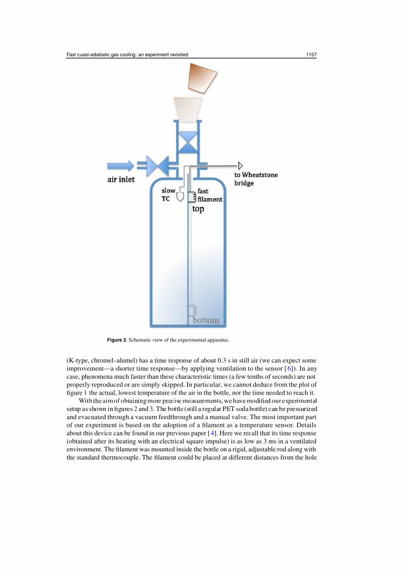
Figure 2. Schematic view of the experimental apparatus.
(K-type, chromel–alumel) has a time response of about 0.3 s in still air (we can expect some
improvement—a shorter time response—by applying ventilation to the sensor [6]). In any
case, phenomena much faster than these characteristic times (a few tenths of seconds) are not
properly reproduced or are simply skipped. In particular, we cannot deduce from the plot of
figure 1 the actual, lowest temperature of the air in the bottle, nor the time needed to reach it.
With the aim of obtaining more precise measurements, we have modified our experimentalsetup as shown in figures 2 and 3. The bottle (still a regular PET soda bottle) can be pressurized
and evacuated through a vacuum feedthrough and a manual valve. The most important part
of our experiment is based on the adoption of a filament as a temperature sensor. Details
about this device can be found in our previous paper [4]. Here we recall that its time response
(obtained after its heating with an electrical square impulse) is as low as 3 ms in a ventilated
environment. The filament was mounted inside the bottle on a rigid, adjustable rod along with
the standard thermocouple. The filament could be placed at different distances from the hole

8/12/2019 Fast Quasi-Adiabatic Gas Cooling: An Experiment Revisited
http://slidepdf.com/reader/full/fast-quasi-adiabatic-gas-cooling-an-experiment-revisited 5/12
1158 G Calza et al
Figure 3. Experimental setup.
of the bottle. The filament was electrically connected to a Wheatstone bridge whose output
was measured with an ADC card (16 bit, data taken at 100 kHz sampling rate).
This experiment, as related above, is usually exploited to describe the fast cooling of air
and the condensation of water vapour included in it. Yet, in our setup we use dry air (N 2), i.e.
we avoid from the very beginning the phenomenon of energy exchange between air and water
vapour. This has been done since our theoretical, didactical model presented and discussed
in the following section would have required a much more complex onset for including a
two-phase component (gaseous and liquid) with its energy balance. Moreover, the main aim
of this work is related to the study of the fast time response of our sensing unit and not to
thermodynamic and gas dynamics details that are beyond levels appropriate to high-school or
introductory college physics.
We show in figure 4 (blue line) a typical output of temperature versus time as obtained
with the filament close to the bottle hole. The first, relevant point is that the temperature drop
is very fast (less than 1/10 s) and quite deep (from 23 ◦C to about −40 ◦C, i.e. a 63 ◦C jump,to be compared with the 25 ◦C value measured with the commercial thermocouple). In figure
4, we also report a second temperature measurement obtained with the filament placed as
close as possible to the bottle bottom, i.e. far from its hole (red line). We observe that the
time required to reach the lowest temperature is again a very short one, but the corresponding
temperature value is definitely higher than that in the previous case. We will comment more
on this in the following section. Figure 4 also shows a complex behaviour of temperature as
time goes by to larger and larger values. Quite close to the minimum temperature, and within a

8/12/2019 Fast Quasi-Adiabatic Gas Cooling: An Experiment Revisited
http://slidepdf.com/reader/full/fast-quasi-adiabatic-gas-cooling-an-experiment-revisited 6/12
Fast quasi-adiabatic gas cooling: an experiment revisited 1159
Figure 4. Temperature versus time of dry air expansion (filament in the top position, blue/black,
bottom, red/grey). Note the logarithmic timescale.
few seconds, we systematically observe very fast, non-random temperature oscillations (in the
range of a few hundreds of seconds) as well as slower changes (in the tenths of seconds range).
We also note a much slower, average temperature rising as time reaches the several seconds
range. We believe that the very fast oscillations close to the minimum temperature are caused
by turbulent flow motions and gas shock-waves inside the bottle, while the overall, slower
temperature increase is associated with the thermal adjustment caused by several, complex
heat exchange processes between the gas inside the bottle and its walls as well as by the mixing
with external air entering the bottle. In the following section, we will present a theoretical
model capable of justifying the rapid temperature drop to the observed minimum value by
combining two basic aspects of the gas transformation: its quick expansion (and cooling) and
its simultaneous, continuous heating. We will not attempt to describe the above-mentioned,
fine structures at a longer timescale for our experiment, since such treatment is far beyond the
purpose of this work (and of standard undergraduate physics courses).
The notable result here is that we have experimentally obtained a clear figure of the
characteristic time for the gas to cool down to its lowest temperature as a consequence of
its fast expansion. Fine observable details of its irreversible, turbulent behaviour are also
accessible in this experiment despite its very simple setup.
Theory
If it is true that the detailed behaviour of the air inside the bottle is an extremely complex event
based on non-reversible, turbulent flows of a real gas, it is, however, possible to obtain some
general information in terms of relatively simple theoretical considerations. Since these ideasmake use of classical thermodynamics concepts at the introductory college physics level, we
think it is worth spending some time on this.
In our experiment, as already discussed, we observe the fast, continuous temperature drop
of the air in the bottle after its opening anda subsequent, much less regular temperature increase
during its exposure to the surrounding media (walls of the bottle and external atmosphere).
Here we show that the first of these two trends can be described fairly well in terms of
an adiabatic gas expansion through a convergent nozzle (the bottle hole). In the following

8/12/2019 Fast Quasi-Adiabatic Gas Cooling: An Experiment Revisited
http://slidepdf.com/reader/full/fast-quasi-adiabatic-gas-cooling-an-experiment-revisited 7/12
1160 G Calza et al
discussions and computations, temperatures are obviously in kelvin. However, to allow a more
intuitive understanding of the results, values are always converted into Celsius.
In a simple, stationary (and reversible) representation of the adiabatic cooling/expansion
of an ideal gas, one obtains the final temperature associated with a pressure ratio ( p1 / p2)
according to
T 1/T 2 = ( p1/ p2)γ −1γ . (1)
In the case of our experiment, we started with air in the bottle pressurized to the value p1 = p0 = 4 × 10⁵ Pa at the initial temperature T 1 = T 0 = 23 ◦C. So, we readily obtain, for
the depressurization to p2 = pfin = patm = 105 Pa, T 2 = T fin = T 0( patm / p0)2/7 = −74 ◦ C, in
which we use γ = cP / cV = 7/5 for a bi-atomic ideal gas. In other words, the gas, being
adiabatically expanded to the atmospheric pressure, undergoes a temperature drop of 97 ◦C
(from about 23 to −74 ◦C). This result, which is the ideal limit for a full adiabatic, reversible
transformation, does not explain the time evolution of our experiment, i.e. does not provide
any information concerning the rapidity with which the temperature drops to a new value after
the gas expansion to the atmospheric pressure.
So, we consider the specific way in which the gas leaves the bottle, i.e. through the hole(nozzle) which is almost instantaneously opened in our experiment. We show in the following
that one can adopt the model of an isoentropic flow (i.e. adiabatic, stationary, non-dissipative)
of a compressible, ideal fluid [7]. Energy dissipation can be left out if the flow is characterized
by relatively large Reynolds numbers, so that viscous forces are negligible in comparison to
other interactions. Under these conditions, one can adopt, as a starting, pilot equation, the
Bernoulli relation for unit mass,
u2
2+ h = const, (2)
in which we omit volume forces (such as gravitational effects) and introduce the specific
enthalpy, h. Equation (2) is computed along a given streamline of the fluid with speed u.
Before considering the problem at issue, i.e. the efflux of gas through the nozzle, we
modify the Bernoulli equation by choosing, as a specific coordinate for our computation, thestagnation point of the gas, which is characterized by the condition u = u0 = 0. If one writes
the specific enthalpy h as h = cPT , and by referring to stagnation point values with the subscript
‘0’, equation (2) can be manipulated to give
u =
2cPT 0
1 − T
T 0
1/2
. (3)
Introducing the speed of sound in the gas a = √ γ RT (here R is the gas constant referred to
the molar unit) and the adiabatic relation between temperature and pressure, equation ( 1), one
obtains
u = a0
2
γ − 1
1 −
p
p0
γ −1γ 1/2
, (4)
which is also known as the Saint-Venant and Wentzel equation [8]. This expression allows usto compute the speed of gas at pressure p starting from the speed of sound a0 =
√ γ RT 0 and
the gas pressure both under stagnation conditions (u = u0 = 0, p0).
It is possible to exploit equation (4) to compute the mass flow through the nozzle with
area A by simply developing the basic definition:
dm
dt = ρuA, (5)

8/12/2019 Fast Quasi-Adiabatic Gas Cooling: An Experiment Revisited
http://slidepdf.com/reader/full/fast-quasi-adiabatic-gas-cooling-an-experiment-revisited 8/12
Fast quasi-adiabatic gas cooling: an experiment revisited 1161
in which we manipulate the density ρ = ρ0(ρ/ρ0) = γ p0
a20
p
p0
1/γ to write
dm
dt = p0
a0
Aeff . (6)
In this expression, we introduce the effective nozzle area Aeff , which is given by
Aeff = A
2γ 2
γ − 1
p
p0
2/γ 1 −
p
p0
(γ −1)/γ 1/2
. (7)
It is customary to introduce the ‘efflux coefficient’ defined as
ψ = ψ( p, p0) =
2γ 2
γ − 1
p
p0
2/γ 1 −
p
p0
(γ −1)/γ 1/2
(8)
in such a way that equation (7) becomes Aeff = Aψ [9]. A very important result of gasdynamics
studies is that the efflux coefficient, despite its variability as a function of local thermodynamic
properties of the fluid, attains its maximum value for the so-called critical conditions of speed,
temperature and pressure (denoted as u∗, p∗ and T ∗). Such conditions correspond to the sonic
speed of gas, i.e. when u
=u∗
=a (the speed of gas equals the speed of sound under the same
conditions), that is, M = M ∗ = 1, where M = u / a is the Mach number. We thus obtain thatunder critical conditions the efflux coefficient is simply given by
ψ∗ = ψmax = γ
2
γ + 1
γ +1
2(γ −1)
, (9)
which, for an ideal bi-atomic gas, is ψ ∗ = 0.82.
We will now make use of this result in considering the outflow of air from the bottle.
This can be done since, for pressure ranges similar to those of our experiment, the speed of
gas in the convergent nozzle is a fraction (about 0.6–0.8) of the speed of sound. So, the efflux
coefficient is close to its maximum value and we write, in place of equation (7), Aeff = Aψ ∗ .
In order to apply the above results to our case study, we consider a bottle whose volume
V B is much larger than the volume V N of the exit nozzle. In our model, we take the air in
the bottle under stationary stagnation conditions, i.e. its pressure, density and temperature
change with time, but the speed of fluid is negligibly small. (This can be justified since the
fluid acquires speed almost entirely in the exit nozzle and not in the bottle volume.) So, the
varying, stagnation coordinates of the air in the bottle are p0(t ), ρ0(t ) and T 0(t ).
The conservation of air mass in the bottle/nozzle system (m B+m N = constant) can now
be explicitly written as
0 = dm
dt = dm B
dt + dm N
dt = V B
dρ0
dt + p0
a0
Aeff . (10)
We modify this last equation by explicitly introducing p0 and T 0. We thus obtain
V B√ R
d
dt
p0
T 0
+ Aeff √
γ
p0√ T 0
= 0. (11)
If we describe the air outflow according to an adiabatic transformation, once again p0 and
T 0 are related to each other by means of the equation T 0/T 0i = ( p0/ p0i)γ −1γ , where we
introduce the initial (t = 0) stagnation values for temperature/pressure, T 0i = T 0(t = 0), p0i = p0(t = 0).
The differential equation (11), in the adiabatic hypothesis, is analytically solved to provide
the following expressions for the stagnation pressure and temperature time dependences:
p0(t ) = p0i
1 + γ − 1
2
t
τ
2γ
1−γ
, (12)

8/12/2019 Fast Quasi-Adiabatic Gas Cooling: An Experiment Revisited
http://slidepdf.com/reader/full/fast-quasi-adiabatic-gas-cooling-an-experiment-revisited 9/12
1162 G Calza et al
Figure 5. Comparison between computed adiabatic temperature drop of dry air (thin lines) and
observed data (thicklines)for the two filament positions (top, blue/black; bottom, red/grey). Note
the linear timescale.
T 0(t ) = T 0i
1 + γ − 1
2
t
τ
−2
(13)
in which we introduce the characteristic time
τ = V B
Aeff
γ
RT 0i
. (14)
Since the final value of the gas stagnation pressure is patm, a known value, we can use
equation (12) to determine the time needed for the gas to reach such a final state (whose
temperature, as already discussed, is T fin = T 0( patm / p0)2/7 = −74 ◦C).
By direct inversion of equation (12), we simply obtain for the time of adiabatic cooling:
t cool =2τ
γ − 1
p0i
patm
γ −1
2γ
− 1
, (15)
which, for our experiment ( p0i / patm = 4), is equal to 1.09 τ . It is easy to obtain that, for t =t cool, equation (13) gives back the expected final temperature, T fin.
The first, direct comparison between the theory and experiment is shown in figure 5 in
which the adiabatic cooling curve given by equation (13) is plotted along with the measured
temperature in the first few tenths of seconds after the opening of the bottle. In this same
figure, we report the two cases for the sensing unit close to and far from the exit nozzle of the
bottle. The theoretical curves have been adjusted by changing the effective nozzle area ( Aeff )
to determine τ in equation (14). Using a smaller, effective area of the exit hole is equivalent
to assuming that, in order to reach the bottom of the bottle, the information associated with its
uncorking must travel a longer, higher impedance path. The adjustment of the parameter hasbeen done by comparing the initial slope of the cooling curves. Starting from equations ( 13)
and (14), one obtains
dT 0
dt (t = 0) = 1 − γ
V B
RT 3
0i
γ Aeff . (16)
By inserting the proper numerical values in the expression above, and the fitted slopes
of the cooling curves (dT 0 /dt (t = 0) = −646 ◦C s−1 and −1226 ◦C s−1, at the bottom and

8/12/2019 Fast Quasi-Adiabatic Gas Cooling: An Experiment Revisited
http://slidepdf.com/reader/full/fast-quasi-adiabatic-gas-cooling-an-experiment-revisited 10/12
Fast quasi-adiabatic gas cooling: an experiment revisited 1163
top filament positions, respectively), we obtain the corresponding Aeff values as well as the
effective, reduced nozzle radius according to
r eff =
A/π =
Aeff /(πψ∗). (17)
Its values, going again from bottom to top, are 3.2 and 4.5 mm, respectively. These valuesshould be compared with the actual, geometric radius of the exit nozzle of the bottle used in
the present experiment, which is 8 mm. These differences, as already hinted, are due to the
actual behaviour of the nozzle in comparison with the ideal hole. An important point is that in
the two reported measurements the minimum value of the temperature is definitely higher than
the adiabatic computed value. This effect is more pronounced in the case of ‘bottom’ filament
positioning: this is expected since here the gas has a longer time to exchange energy with
the warm bottle’s walls. However, our computation is in good agreement with the observed
temperature drop in the first, quick phase of the gas expansion (0–0.1 s). Equations ( 14) and
(15) provide for the cooling time 10.4 and 20.7 ms for the filament at the top and bottom
positions, respectively.
The adiabatic minimum is not reached since the air in the bottle is continuously heated
from the very beginning, mainly because of its contact with the warmer bottle’s walls. We
account for this fact with a very simple conduction/convection model for energy exchange by
means of which the adiabatic behaviour will be corrected. We consider the external air as an
infinite thermal capacity, energy source at fixed temperature T air (23 ◦C in our experiment).
The walls of the bottle are also at this same temperature and we suppose that they do not
change this status as a consequence of their contact with the cold internal air. This assumption
is supported by the quickness of the gas cooling and by the fact that the thermal inertia of the
wall material (PET plastic) is large enough to ensure a much slower temperature adjustment.
So, the only way for the internal air to acquire heat from outside is by means of convective
energy transfer from the walls at constant temperature.
We consider, for the system constituted by the bottle and the nozzle, the following equation
for the energy conservation:
d(m BU B)
+h N dm N
=δQ, (18)
in which the first term on the left-hand side represents the change of internal energy of the air
in the bottle, while the second term is related to the flow of enthalpy through the nozzle. Being
that air is flowing from the bottle to the nozzle, one has that dm B = −dm N = dm. We thus can
write, putting U = U B and h = h N = U + pV :
mdU + U dm − hdm = dm(U − h) + mdU = mdU − pV dm. (19)
By replacing mass values with molar quantities andreferring the above equationsto the number
of moles n(t ), we obtain
ncV dT − RT dn = δQ. (20)
As a final step, we consider stagnation values for the number of moles and of temperature, and
instantaneous values:
n0cV dT 0dt
− RT 0 dn0dt
= Q. (21)
The thermal flux of energy Q is expressed by means of the convection/conduction law for a
fluid at temperature T 0 in contact with a wall (surface S ) at temperature T W , Q = k cS (T W − T 0) z.
In this formula, k c is the effective convection constant for the gas–wall heat transmission and
the exponent z is empirically settled in the function of the (complex) characteristics of the
convection geometry and dynamics [10]. The value of k c is usually obtained from a class of
typical experimental configurations. In our case, the walls are those of the bottle, with the

8/12/2019 Fast Quasi-Adiabatic Gas Cooling: An Experiment Revisited
http://slidepdf.com/reader/full/fast-quasi-adiabatic-gas-cooling-an-experiment-revisited 11/12
1164 G Calza et al
Figure 6. Comparison between observed data (thick lines) and theoretical model (equations (22)
and (23), thin lines) for the two different filament locations (top, blue/black; bottom, red/grey).
Note the logarithmic timescale.
surface S B , and the temperature will be that of the outside air, as explained above. We are
thus left with the energy balance differential equation relating density (number of moles) and
temperature of the internal air at stagnation points:
n0cV
dT 0
dt − RT 0
dn0
dt = k cS B(T air − T 0)
z. (22)
The differential equation for the gas outflow, equation (11), can be written in terms of the
number of moles under the stagnation conditions, n0, in place of the associated gas pressure,
p0, with the result being
dn0
dt + Aeff
V B
Rγ
n0
T 0 = 0. (23)
This last equation, along with equation (22), constitutes the system of differential equations
leading to the time dependences of relevance here, i.e. n0(t ) and p0(t ). A numerical approach
to this problem is convenient since the nonlinear form of these equations strongly discourages
any attempt to seek for analytical solutions.
So, we proceed with the numerical integration of equations (22) and (23). We show in
figure 6 the results of this computation along with the observed data for the two different
filament positions. The convective parameter k c of equation (22) has been fixed to the value
70 W m−2 K−1 (according to ‘recommended’ figures for air convection phenomena [10]), but
one could slightly change such values without affecting the overall aspect of the computed
curve too much. The exponent z, according to the literature, is in the 1–1.5 range [11]. We
chose, quite arbitrarily, z = 1.3. We observe that the overall agreement between experimentand our model is fair. There is evident discrepancy in the case of the filament located at
the bottom of the bottle where, as already discussed, we expect a more complex and less
predictable behaviour because of the (basically unknown) detailed dynamics of the expanding
air. However, thelowest temperature reached as well as thetime required to obtainthis value are
well described, with our model, in the ‘top’ configuration. The gas heating has been modelled
in such a way that only the minimum reached temperature and the associated cooling time
have been reproduced fairly well: the subsequent, longer timescale behaviour of temperature

8/12/2019 Fast Quasi-Adiabatic Gas Cooling: An Experiment Revisited
http://slidepdf.com/reader/full/fast-quasi-adiabatic-gas-cooling-an-experiment-revisited 12/12
Fast quasi-adiabatic gas cooling: an experiment revisited 1165
(along with its fine, shorter timescale details) are definitely beyond the predictive possibilities
of this model.
Conclusion
Since the main aim of this work was to show the fast time responsiveness of our temperature
sensor, we think that the filament is a very well-suited device in this respect. We have observed
very complex, still repeatable oscillations in the few-millisecond scale of the temperature
change of dry air expansion within our bottle. Moreover, the theoretical model presented here
is capable of reproducing the first phases of the experiment with quite good accuracy, i.e. the
dry gas cooling, with a cooling time of about 0.1 s for our setup. The minimum temperature is in
the −40 to −60 ◦C range, showing that the pure adiabatic limit is quite far from being reached.
A fair adjustment of this ideal limit is achieved by allowing energy exchange via effective
convective processes with the bottle walls. The overall solution of the resulting differential
equations is compatible with the observed values of minimum temperature and the associated
cooling time. It could also be that exchanges of electromagnetic radiation because of the finite
temperature difference between the filament and the surrounding environment would play acertain role in our experiment. We have modelled a classical εσ T 4 energy exchange term in
our computation. The result is that there is a net energy flow of electromagnetic origin such
that a difference of temperature of up to 3–4 ◦C is accounted for between the filament and the
expanding gas. Such a phenomenon, however, does not modify our main conclusions, since
the time within which the filament starts to warm up (following a thermal radiation process as
a consequence of its lowered temperature because of the gas cooling) is of the order of 0.5 s,
i.e. too long to be relevant in the first, rapid phase of our experiment.
Acknowledgment
We thank Professor G M Carlomagno at the Aerospace Engineering Department in Naples,
Italy for useful discussions and comments.
References
[1] GuemezJ, Fiolhais C and FiolhaisM 2007 Physics of the fire piston and the fog bottle Eur. J. Phys. 28 1199–205Graham M T 2004 Cloud formation Phys. Teach. 42 301–4Bohren C F 1987 Clouds in a Glass of Beer (New York: Wiley)
[2] Zukrow M J 1948 Principles of Jet Propulsion and Gas Turbines (New York: Wiley)[3] Bohren C F and Albrecht B A 1998 Atmospheric Thermodynamics (Oxford: Oxford University Press)[4] Calza G, Gratton L M, Lopez-Arias T and Oss S 2012 Very fast temperature measurement with a thin lamp
filament Phys. Educ. 47 334–7[5] Coop J J 1941 A demonstration of fog production Am. J. Phys. 9 242[6] Haman K E, Makulski A and Malinowski S P 1997 A new ultrafast thermometer for airborn measurements in
clouds J. Atmos. Ocean. Technol. 14 217–27[7] Batchelor G K 2005 An Introduction to Fluid Dynamics (Cambridge: Cambridge University Press)[8] Sedov L I 1997 Mechanics of Continous Media vol 2 (Singapore: World Scientific)
[9] Ziegler F 1995 Mechanics of Solids and Fluids (New York: Springer)[10] Bohren C F 2011 Why do objects cool more rapidly in water than in still air? Phys. Teach. 49 550–3[11] Cengel Y A 2008 Introduction to Thermodynamics and Heat Transfer (New York: McGraw-Hill)