Abstract— In this paper, we automate the traditional problem of Simultaneous Localization and Mapping (SLAM) by interleaving planning for exploring unknown environments by a mobile robot. We denote such planned SLAM systems as SPLAM (Simultaneous Planning Localization and Mapping). The main aim of SPLAM is to plan paths for the SLAM process such that the robot and map uncertainty upon execution of the path remains minimum and tractable. The planning is interleaved with SLAM and hence the terminology SPLAM. While typical SPLAM routines find paths when the robot traverses amidst known regions of the constructed map, herein we use the SPLAM formulation for an exploration like situation. Exploration is carried out through a frontier based approach where we identify multiple frontiers in the known map. Using Randomized Planning techniques we calculate various possible trajectories to all the known frontiers. We introduce a novel strategy for selecting frontiers which mimics Fast SLAM, selects a trajectory for robot motion that will minimize the map and robot state covariance. By using a Fast SLAM like approach for selecting frontiers we are able to decouple the robot and landmark covariance resulting in a faster selection of next best location, while maintaining the same kind of robustness of an EKF based SPLAM framework. We then compare our results with Shortest Path Algorithm and EKF based Planning. We show significant reduction in covariance when compared with shortest frontier first approach, while the uncertainties are comparable to EKF-SPLAM albeit at much faster planning times. Index Terms – SPLAM, Exploration, trajectory Planning, FastSLAM.

I. INTRODUCTION

HE problem of SLAM involves estimating the state of the robot and map simultaneously and concurrently.

Long considered the holy grail in mobile robotic systems there now exist several matured algorithms for SLAM [12]. Most SLAM maps are built by remotely controlling or teleoperating the robot. Often the human in loop uses his vast experience by appropriately driving the vehicle in a fashion so that the uncertainty of the whole system represented often through its covariance matrix does not explode or grow beyond bounds. For example it is common practice to to keep the robots close to landmarks that has already been seen to keep the error covariance so as to speak within control. This transfer of human experience onto a planner is a critical step in automation of SLAM. A fully automated SLAM system must decide where next to move to

*Students at Robotics Research Center at IIIT Hyderabad. Names

arranged in alphabetical order for students +Faculty with the Robotics Research Center, IIIT Hyderabad.

continue the process mapping, often called exploration. Most exploration systems involve finding regions known as frontiers [1] and finding the best frontier to move. Often the best frontier is one that is shortest [1] or one of maximal information gain [2], [3].

However in SLAM automation or SPLAM systems the critical criterion has typically been to consider state covariance more than anything else as the deciding factor where to move [4], [6]. The trace or the determinant of the covariance often indicates the amount of uncertainty of the state and is used in the automation policy. While the path that churns out the least possible uncertainty value can seldom be found due to the exponential nature of the search involved, most paths obtained as an outcome of the SLAM process do show reduced uncertainty in state during and at the end of the robot’s sojourn.

Most methods that perform SPLAM use an EKF framework [4], [5], which essentially involves computing the full state covariance for a finite time horizon over a future path. Later SPLAM was modified into an Active SLAM framework in [6]. The path that provides the least covariance trace is selected as the best possible path. However computing the full state covariance for a finite time horizon is computationally unwieldy especially as the number of landmarks increase. The full state covariance considers all possible correlations between landmark and robot poses that tends to be the main cause of computational bottleneck.

Herein we propose an alternate fast randomized planner that interleaves planning into SLAM framework. Multiple paths are generated to each frontier location and further each path is estimated by a certain small number of particles [11]. Since the entire path to the frontier is now assumed known it is mathematically sound to decouple the landmark and robot state covariances [7]. This results in a much faster planner when compared with a planner operating on a full covariance matrix. A new metric that weighs both landmark and robot state uncertainty vis-à-vis distance is used to compute the best possible path in terms of reduced uncertainty of map and robot states.

It is well known that maps and trajectories resulting from a Fast SLAM like sampling process is not as robust as EKF SLAM [7]. To combine advantages of both we use a sampling based planner with Fast SLAM like decoupling of landmark states while retaining the EKF-SLAM [10] for the baseline SLAM framework. In other words when the robot moves to a new location its update is based on EKF SLAM while the path to that location is based on a planner with

Fast Randomized Planner for SLAM Automation

Amey Parulkar*, Piyush Shukla*, K Madhava Krishna+

T

decoupled states. We show several results that vindicate the efficacy of the

proposed method. In particular we show significantly reduced planning times and comparable robustness via-a-vis an EKF based SPLAM. Also shown is that the proposed planner is far more robust than one that selects a path, which is merely the shortest to frontiers.

II. RELATED WORK

One of the well-known methods in SPLAM literature is due to Dissanayake’s group [4]. The method proposed a finite time look ahead based planning for EKF-SLAM baseline. The method dealt with the full covariance matrix throughout the planning stage. Later the method was cast into a Model Predictive Control Paradigm (MPC) in [5] while still working with the full covariance matrix. Whereas in [6] a new criterion for optimality called A-optimality within SPLAM was proposed. The paper in effect showed how considering the trace rather than the determinant of the covariance matrix as an appropriate metric gave better results. In [8] a Bayesian framework was proposed to decouple the localization, planning and control problem and showed how a planning problem becomes one of stochastic control under bounded uncertainty. However the paths shown therein were under a localization than SLAM framework. In [9] an exploration for SLAM was proposed that considered several heuristics while selecting a path. Essentially the theme was to select locations from where already seen landmarks would be visible to prevent uncertainty growth. However this work failed to integrate the exploration with SLAM and did not bring in explicitly uncertainty based formalism and metrics while computing the paths

The current work contrasts in bringing about an integration of a faster but robust sampling based planner into a baseline EKF-SLAM based SPLAM thereby availing benefits of both. The work is supported by extensive simulation results, comparisons and real experiments.

III. OVERVIEW

In this section, we provide an overview of the proposed

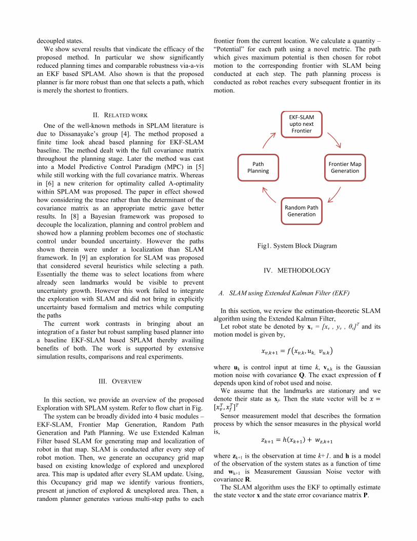
Exploration with SPLAM system. Refer to flow chart in Fig. The system can be broadly divided into 4 basic modules –

EKF-SLAM, Frontier Map Generation, Random Path Generation and Path Planning. We use Extended Kalman Filter based SLAM for generating map and localization of robot in that map. SLAM is conducted after every step of robot motion. Then, we generate an occupancy grid map based on existing knowledge of explored and unexplored area. This map is updated after every SLAM update. Using, this Occupancy grid map we identify various frontiers, present at junction of explored & unexplored area. Then, a random planner generates various multi-step paths to each

frontier from the current location. We calculate a quantity – “Potential” for each path using a novel metric. The path which gives maximum potential is then chosen for robot motion to the corresponding frontier with SLAM being conducted at each step. The path planning process is conducted as robot reaches every subsequent frontier in its motion.

Fig1. System Block Diagram

IV. METHODOLOGY

A. SLAM using Extended Kalman Filter (EKF)

In this section, we review the estimation-theoretic SLAM

algorithm using the Extended Kalman Filter, Let robot state be denoted by xv = [xv , yv , θv]

T and its motion model is given by,

, , , , . where uk is control input at time k, vu,k is the Gaussian motion noise with covariance Q. The exact expression of f depends upon kind of robot used and noise.

We assume that the landmarks are stationary and we denote their state as xf. Then the state vector will be

, Sensor measurement model that describes the formation

process by which the sensor measures in the physical world is,

, where zk+1 is the observation at time k+1. and h is a model of the observation of the system states as a function of time and wk+1 is Measurement Gaussian Noise vector with covariance R.

The SLAM algorithm uses the EKF to optimally estimate the state vector x and the state error covariance matrix P.

EKF‐SLAM upto next Frontier

Frontier Map Generation

Random Path Generation

Path Planning

The EKF-SLAM algorithm is divided into 2 stages- 1. The prediction stage involves updating the state mean and variance after a movement. This is done using the control information and the process error variance.

\ , ,0

| | where Fk ,Gk are Jacobians of f with respect to x and vu,k evaluated at , ,0 , respectively. 2. The update stage uses the acquired information of associated features extracted from sensor readings to simultaneously update the robot pose and the map.

| | |

| | Where,

| |

Where Hk is the Jacobian of h evaluated at | .

B. Frontier Map Generation

After every iteration of SLAM, we generate a occupancy

grid map of the environment. It uses the laser sensor scan data to create grid based map that shows explored and unexplored region in the surroundings of robot. While, this same laser data is used by SLAM to show landmark positions, here it is used to identify frontiers.

C. Random Path Generation

The next task is to select the next frontier and to plan an optimum trajectory for reaching there, such that we minimize error in robot and map states as the robot reaches the frontier. We employ a random path generator algorithm that generates a finite number of paths from current location to all the known frontiers. Around 15-20 paths are generated for each of the frontier destinations. These paths have step-size and step count constraints. A path can have maximum 10 intermediate nodes, i.e. point where SLAM is conducted, and the maximum distance between two nodes can be 50cms. Also, no two paths generated intersect at any point, this ensures that paths are sparsely distributed and thus cover more possible permutations. All these constraints limit total path length and thus, the choices of frontiers. As a result, chosen frontiers are around about same distance from the current robot location and they have unbiased similar chance of being selected. Finally, we have to select the optimum

trajectory through the proposed planning method as in section. IV.D. The Need for a Planner:

Path planning is important part of Autonomous Localization and Mapping problem by a robot. Since the goal is to explore the unknown surroundings and also at the same time to minimize the landmark and robot uncertainty, we need to find a optimum trajectory which helps achieve this.

One approach to reduce the map uncertainty is to move robot in the known area such that it revisits the good landmarks, with smaller covariance, frequently. This will improve the map but won’t result in any exploration. Thus, for exploration to occur, the robot must be moving in direction of a frontier and at same time taking a path that is in vicinity of many good landmarks to achieve good maps. One of the important requirements is to decide upon a benchmark for measuring the outcome of planning algorithm. This can be done based on two criterions – Final Robot-Map Uncertainty and Total time required for exploration, planning and mapping of entire map. We consider trace of final state matrix, trace (P), as the criterion for measuring accuracy of robot localization and map generation. More is the trace more is the uncertainty in localization and mapping. We keep the baseline SLAM and the frontier generation process to be the same across the methods that are compared. Hence any difference in time is dependent only on how fast planning algorithm is. We have implemented 3 planning algorithms – Shortest path algorithm, EKF based planning and our novel planning algorithm.

D. Fast Planning Algorithm

A Planning algorithm is basically a simulation of robot

motion along all possible paths with SLAM being conducted at each step. A criterion quantity – ‘Potential’ decides the quality of SLAM outcome at end of each path. Thus, main aim of planning algorithm is to speculate which path will give the best possible SLAM state on reaching the next frontier. This speculation is done based on the information available till now. This is so because during simulation we don’t actually move the robot and conduct SLAM updates. Thus, we cannot see any new landmarks and have to make our decision based on presently explored map. Due to this constraint, it becomes important to use an efficient planning algorithm that can give good paths. Also, for this system to run in real-time on a robot, it must be considerably fast.

All the above discussed parameters are considered in our Fast Planning algorithm. Initially, the robot pose, as obtained from EKF-SLAM state, is sampled into M particles and we consider separate maps for each particle. It means that each particle has its own state and correspondingly all landmark’s mean and covariances associated with it. This decoupling of landmark and robot state precludes the need for bulky

(2N+3) X (2N+3), P matrix. Instead we have N-2X2

matrices associated with each of the M particles. These N-2X2 matrices are covariance matrices of N landmarks, which can be taken from P matrix. Decoupling procedure will significantly reduce the computational complexity as

calculations involving small matrices are lot faster that that on larger matrices especially, the inverse.

Next, we conduct a modified fastSLAM for all the trajectories derived from random path generator. This involves traditional fastSLAM prediction, update and resampling being done at each and every node on all the trajectories. We employ a novel way to calculate weights of particles after every update. It is given as the ratio of previous weight to the sum of trace of visible landmark covariances from that particle. This approach will give more weights to particles which can see good landmarks, i.e. with less trace. Thus, particles which are close to good landmarks have higher weights and are more likely to be selected in resampling stage. Finally, we introduce a quantity - ‘Path Potential’, sum of inverse of trace of all the visible landmarks averaged over all particles for all the nodes. This quantity determines, on an average, quality of landmarks visible when moving through a particular trajectory. Higher Path Potential for a trajectory suggests that, this trajectory approaches more good landmarks and so if robot moves along this trajectory then it has better chance of obtaining good SLAM states.

V. RESULTS

We have implemented three Exploration with SPLAM

methods for comparing results. All these methods have common EKF-SLAM, Frontier Map Generator and Random Path Generator implementations. They each have different Planning algorithm – 1) shortest-path planning algorithm, that always finds the shortest path from current location to the next frontier. 2) EKF based planning algorithm as in [4]. 3) the fast randomized planner of this paper. All these algorithms were implemented on Matlab, while some of the library functions of C were also used.

The exploration with SPLAM system was tested rigorously on simulation by changing the simulation environments and system variables. Performance was analysed on basis of accuracy and time taken. The measure of accuracy is done by calculating the trace of the covariance matrix at the end, when full map is explored. Fig.3 shows the complete exploration trajectory for all three methods. It is evident that in Fast Planning methods, the trajectories taken are such that good landmarks are visited frequently. Fig.4 shows how the whole frontier map grows during the whole exploration process.

Consider an example of an instance in Planning process as shown in Fig.2. Here, robot is currently at location D, and considers 3 frontiers to visit, A, B and C. Note that not all the three frontiers are visible from D as some of them are frontiers from a previous view that have not yet been visited. Now, the random path generator generates around 15-20 trajectories to each frontier. Fast planning algorithm then identifies a trajectory, in red, that it believes will be best for robot motion to next frontier, C. This path is taken by the robot.

Fast Planning Algorithm (x, P, Path, R, Q) // ‘x’ is SLAM state matrix, ‘P’ is state covariance, ‘Path’ contains all random trajectories, ‘R’ is measurement covariance, ‘Q’ is motion covariance

For each ith random trajectory in path

Sample robot position uncertainty into M particles with, x0

[k] , for k=1 to M // x0[k] is kth particle state at initial

position w0

[k] = probability at x0[k] in Ɲ (x, P)

Generate Y0 by taking landmark covariances from P, Y0 = {x0

[k], (µ1,0[k], Ʃ1,0

[k])………… ,(µN,0[k], ƩN,0

[k])} //for all k

// µ is mean and Ʃ is covariance of Nth landmark pathPotential(i) = 0

for tth node in path(i) Potential = 0 for k=1 to M

Retrieve {xt-1[k], (µ1,t-1

[k], Ʃ1,t-1[k])………… ,(µN,t-

1[k], ƩN,t-1

[k])} from Yt-1

xt[k] ~ p(xt | xt-1

[k], ut) //sample pose J = visible landmarks from xt

[k] //observed feature For all j G = g′ (xt

[k], µj,t-1[k]) //Calculate Jacobian

S = GT Ʃj,t-1[k] G + Rt // measurement

Covariance K = Ʃj,t-1

[k]GS-1 //Kalman Gain µj,t

[k] = µj,t-1[k] //Update mean

Ʃj,t[k] = (I – KGT) Ʃj,t-1

[k] //Update Covariance End Potential = Potential + ∑J 1/trace(Ʃj,t

[k]) wt

[k] = wt-1[k]/∑J trace(Ʃj,t

[k]) for all j not included in J µj,t

[k] = µj,t-1[k]

Ʃj,t[k] = Ʃj,t-1

[k] End End Potential = Potential/M pathPotential(i) = pathPotential(i) + Potential; End pathPotential(i) = pathPotential(i)/size(path(i)) Yt = {} // initial new particle set Do M times // resample M particles Draw random k with probability α w[k] //resample Add {xt

[k], (µ1,t[k], Ʃ1,t

[k])………… ,(µN,t[k], ƩN,t

[k])} to Yt

End End Select path(i) for which pathPotential(i) is maximum

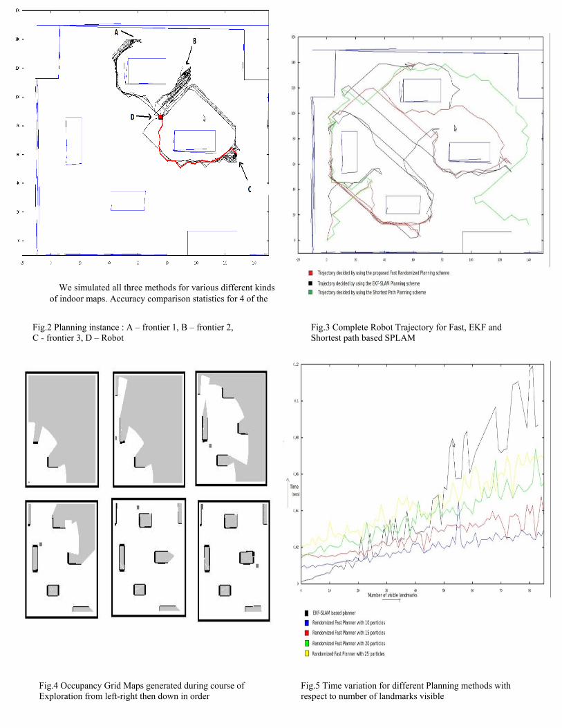
We simulated all three methods for various different kinds of indoor maps. Accuracy comparison statistics for 4 of the

Fig.3 Complete Robot Trajectory for Fast, EKF and Shortest path based SPLAM

Fig.4 Occupancy Grid Maps generated during course of Exploration from left-right then down in order

Fig.5 Time variation for different Planning methods with respect to number of landmarks visible

Fig.2 Planning instance : A – frontier 1, B – frontier 2, C - frontier 3, D – Robot

Maps

Planning Methods Map

Characteristics Shortest

Path SPLAM

EKF SPLAM

Fast SPLAM

Map1

Many landmarks &

Scattered

0.1583

0.15030

0.13940

Map2 Few landmarks & Scattered

0.19611 0.081705 0.050423

Map3

Many landmarks & Clustered at

Center

0.21994

0.072572

0.067625

Map4

Few landmarks & Clustered at

Center

0.36318

0.10424

0.11964

TABLE 1. Trace values of Final Covariance Matrix for 3

different SPLAM methods

Fig.6 Maps obtained after Fast Planner based SPLAM maps is given in Table.1 . As evident from the values in the table, the proposed planner is far more robust than the shortest path based planner and has better or comparative accuracy when compared with the EKF based planner. An important observation to be noted is that, in a map where landmarks are clustered as in Map3 and Map4 (Fig.6), a significant advantage of Fast Planned and EKF Planner can be seen over Shortest path Planner when compared with scattered landmarks as in Map1 and Map2(Fig.6). This happens because in scattered-landmarks maps, almost any trajectory will see significant number of good landmarks but for clustered-landmarks maps, planning trajectory becomes vital as there exist only few locations from where good landmarks can be seen.

We compare time taken for all the three methods considering time taken for planning decision made at nodes. Fig. 5 shows that time varies according to number of visible landmarks, as higher the number of visible landmarks more is the time taken for computing the inverse matrix required in computation of Kalman Gain, in an EKF based planner. Time comparison for Fast Planning method with different particle counts is also shown. It is evident from the figure that Fast Planning method works significantly faster than EKF Planning method.

VI. CONCLUSION

In this paper, we have considered a fast trajectory planning algorithm in Extended Kalman Filter (EKF) based SLAM. The objective is to plan robot’s path in such a way that it completely explores the surrounding environment autonomously and also conduct SLAM simultaneously to finally achieve minimum estimation error. Planning process also has to be fast enough so as to work on robot in real time applications. According to theoretical analysis and as confirmed in simulations, it is evident that our planning algorithm performs much better than the algorithm that visits the closest frontier in terms of robustness of the final estimates of robot path and landmark pose. It shows significant reduction in computational time (planning time) vis-à-vis EKF SPLAM while maintaining the robustness of EKF SPLAM. Thereby it realizes a novel means of automating the SLAM process.

REFERENCES [1] B Yamauchi, ”A frontier-based approach for Autonomous

Exploration”, in IEEE International Symposium on Computational Intelligence in Robotics and Automation, pp 146-151., 1998

[2] W. Burgard, M. Moors, C. Stachniss, and F. Schneider,"Coordinated Multi Robot Exploration", in IEEE Transactions on Robotics, 21(3), 2005.

[3] J. Ko, B. Stewart, D. Fox, K. Konolige, and B. Limketkai, " A Practical, Decision-theoretic Approach to Multi-robot Mapping and Exploration", in IROS, vol 3, pp 3232-3238, 2003

[4] Shoudong Huang, N. M. Kwok, G. Dissanayake, Q.P. Ha, Gu Fang, “Multi-Step Look-Ahead Trajectory Planning in SLAM: Possibility and Necessity”, in Proceedings of the IEEE International Conference on Robotics and Automation Barcelona, Spain, April 2005

[5] Cindy Leung, Shoudong Huang, Ngai Kwok, Gamini Dissanayake, “Planning under uncertainty using model predictive control for information gathering”, in Robotics and Autonomous Systems, pp 898-910, 2006

[6] Cindy Leung, Shoudong Huang and Gamini Dissanayake,, “Active SLAM using Model Predictive Control and Attractor based Exploration”, in Proceedings of IROS 2006, pp 5026-5031

[7] M Montemerlo, S Thrun, D Koller, B Wegbreit, 2002a, “FastSLAM A factored solution to the simultaneous localization and mapping problem”, in Proceedings of the AAAI National Conference on Artificial Intelligence, Edmonton, Canada, AAAI

[8] Andrea Censi, Daniele Calisi, Alessandro De Luca, Giuseppe Oriolo, “A Bayesian framework for optimal motion planning with uncertainty”, in ICRA, pp 1798 – 1805, Pasadena, CA, 2008

[9] Benjamın Tovar, Lourdes Munoz-Gomez, Rafael Murrieta-Cid, Moises Alencastre-Miranda, Raul Monroy, Seth Hutchinson, “Planning exploration strategies for simultaneous localization and mapping”, in Robotics and Autonomous Systems, pp 314–331, 2006

[10] Tim Bailey, “Mobile Robot Localisation and Mapping in Extensive Outdoor Environments”, Ph.D. thesis, Australian Centre for Field Robotics, Department of Aerospace, Mechanical and Mechatronic Engineering, The University of Sydney, 2002.

[11] A. Doucet, J.F.G. de Freitas, N.J. Gordon (Eds.), “Sequential Monte Carlo Methods In Practice”, Springer, New York, 2001.

[12] Cyrill Stachniss, Udo Frese, Giorgio Grisetti, “OpenSLAM”, http://openslam.org/.