Embed Size (px)
Citation preview
useR! 2009 Trevor Hastie, Stanford Statistics 1
Fast Regularization Paths viaCoordinate Descent
Trevor HastieStanford University
joint work with Jerome Friedman and Rob Tibshirani.
useR! 2009 Trevor Hastie, Stanford Statistics 2
Linear Models in Data Mining
As datasets grow wide—i.e. many more features than samples—thelinear model has regained favor in the dataminers toolbox.
Document classification: bag-of-words can leads to p = 20K
features and N = 5K document samples.
Image deblurring, classification: p = 65K pixels are features,N = 100 samples.
Genomics, microarray studies: p = 40K genes are measuredfor each of N = 100 subjects.
Genome-wide association studies: p = 500K SNPs measuredfor N = 2000 case-control subjects.
In all of these we use linear models — e.g. linear regression, logisticregression. Since p� N , we have to regularize.
useR! 2009 Trevor Hastie, Stanford Statistics 3
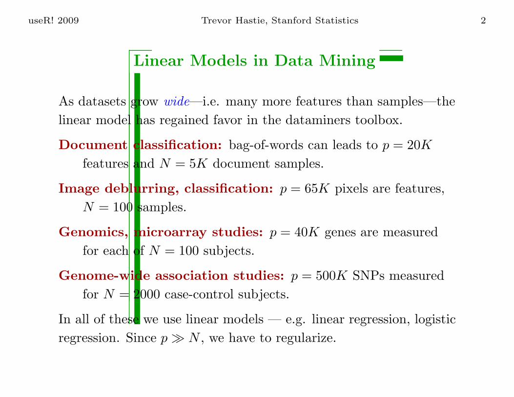
February 2009. Additional chapters on wide data, random forests,graphical models and ensemble methods + new material on pathalgorithms, kernel methods and more.
useR! 2009 Trevor Hastie, Stanford Statistics 4
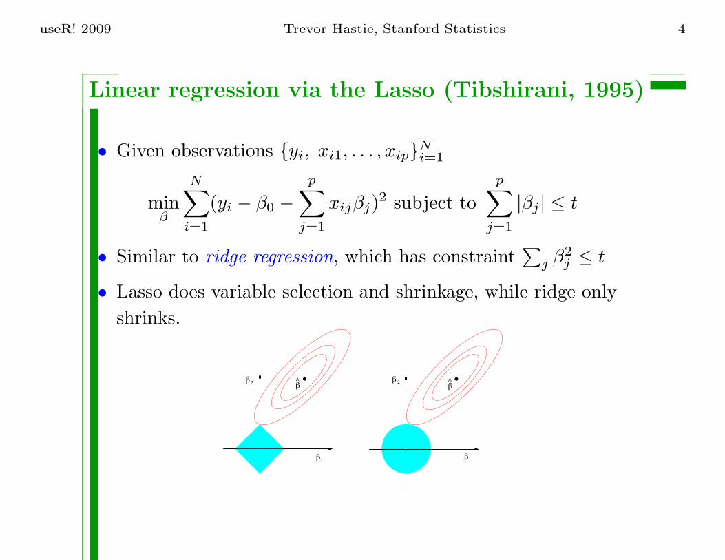
Linear regression via the Lasso (Tibshirani, 1995)
• Given observations {yi, xi1, . . . , xip}Ni=1
minβ
N∑i=1
(yi − β0 −p∑
j=1
xijβj)2 subject top∑
j=1
|βj | ≤ t
• Similar to ridge regression, which has constraint∑
j β2j ≤ t
• Lasso does variable selection and shrinkage, while ridge onlyshrinks.
β^
β^2
. .β
1
β 2
β1
β
useR! 2009 Trevor Hastie, Stanford Statistics 5
Brief History of �1 Regularization
• Wavelet Soft Thresholding (Donoho and Johnstone 1994) inorthonormal setting.
• Tibshirani introduces Lasso for regression in 1995.
• Same idea used in Basis Pursuit (Chen, Donoho and Saunders1996).
• Extended to many linear-model settings e.g. Survival models(Tibshirani, 1997), logistic regression, and so on.
• Gives rise to a new field Compressed Sensing (Donoho 2004,Candes and Tao 2005)—near exact recovery of sparse signals invery high dimensions. In many cases �1 a good surrogate for �0.
useR! 2009 Trevor Hastie, Stanford Statistics 6
0.0 0.2 0.4 0.6 0.8 1.0
−50
00
500
52
110
84
69
0 2 3 4 5 7 8 10
||β̂(λ)||1/||β̂(0)||1
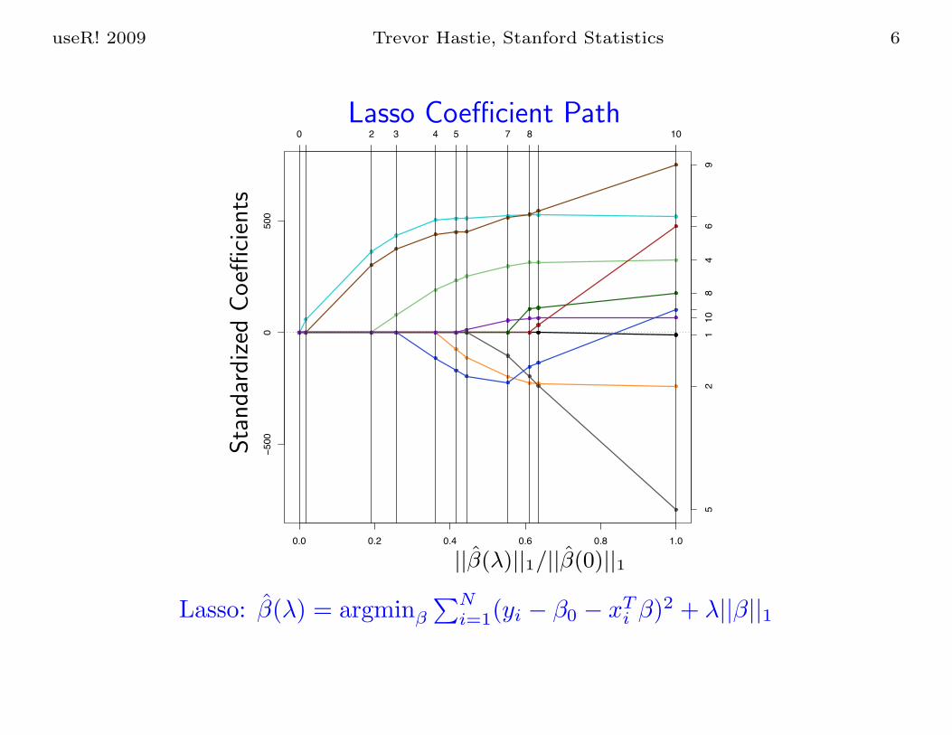
Lasso Coefficient Path
Sta
ndar
diz
edCoeffi
cien
ts
Lasso: β̂(λ) = argminβ
∑Ni=1(yi − β0 − xT
i β)2 + λ||β||1
useR! 2009 Trevor Hastie, Stanford Statistics 7
History of Path Algorithms
Efficient path algorithms for β̂(λ) allow for easy and exactcross-validation and model selection.
• In 2001 the LARS algorithm (Efron et al) provides a way tocompute the entire lasso coefficient path efficiently at the costof a full least-squares fit.
• 2001 – present: path algorithms pop up for a wide variety ofrelated problems: Grouped lasso (Yuan & Lin 2006),support-vector machine (Hastie, Rosset, Tibshirani & Zhu2004), elastic net (Zou & Hastie 2004), quantile regression (Li& Zhu, 2007), logistic regression and glms (Park & Hastie,2007), Dantzig selector (James & Radchenko 2008), ...
• Many of these do not enjoy the piecewise-linearity of LARS,and seize up on very large problems.
useR! 2009 Trevor Hastie, Stanford Statistics 8
Coordinate Descent
• Solve the lasso problem by coordinate descent: optimize eachparameter separately, holding all the others fixed. Updates aretrivial. Cycle around till coefficients stabilize.
• Do this on a grid of λ values, from λmax down to λmin
(uniform on log scale), using warms starts.
• Can do this with a variety of loss functions and additivepenalties.
Coordinate descent achieves dramatic speedups over allcompetitors, by factors of 10, 100 and more.
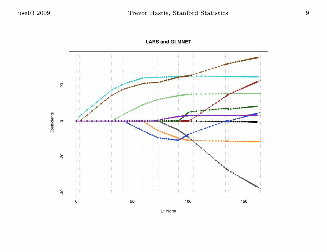
useR! 2009 Trevor Hastie, Stanford Statistics 9
0 50 100 150
−40
−20
020
L1 Norm
Coe
ffici
ents
LARS and GLMNET
useR! 2009 Trevor Hastie, Stanford Statistics 10
Speed Trials
Competitors:
lars As implemented in R package, for squared-error loss.
glmnet Fortran based R package using coordinate descent — topicof this talk. Does squared error and logistic (2- and K-class).
l1logreg Lasso-logistic regression package by Koh, Kim and Boyd,using state-of-art interior point methods for convexoptimization.
BBR/BMR Bayesian binomial/multinomial regression package byGenkin, Lewis and Madigan. Also uses coordinate descent tocompute posterior mode with Laplace prior—the lasso fit.
Based on simulations (next 3 slides) and real data (4th slide).
useR! 2009 Trevor Hastie, Stanford Statistics 11
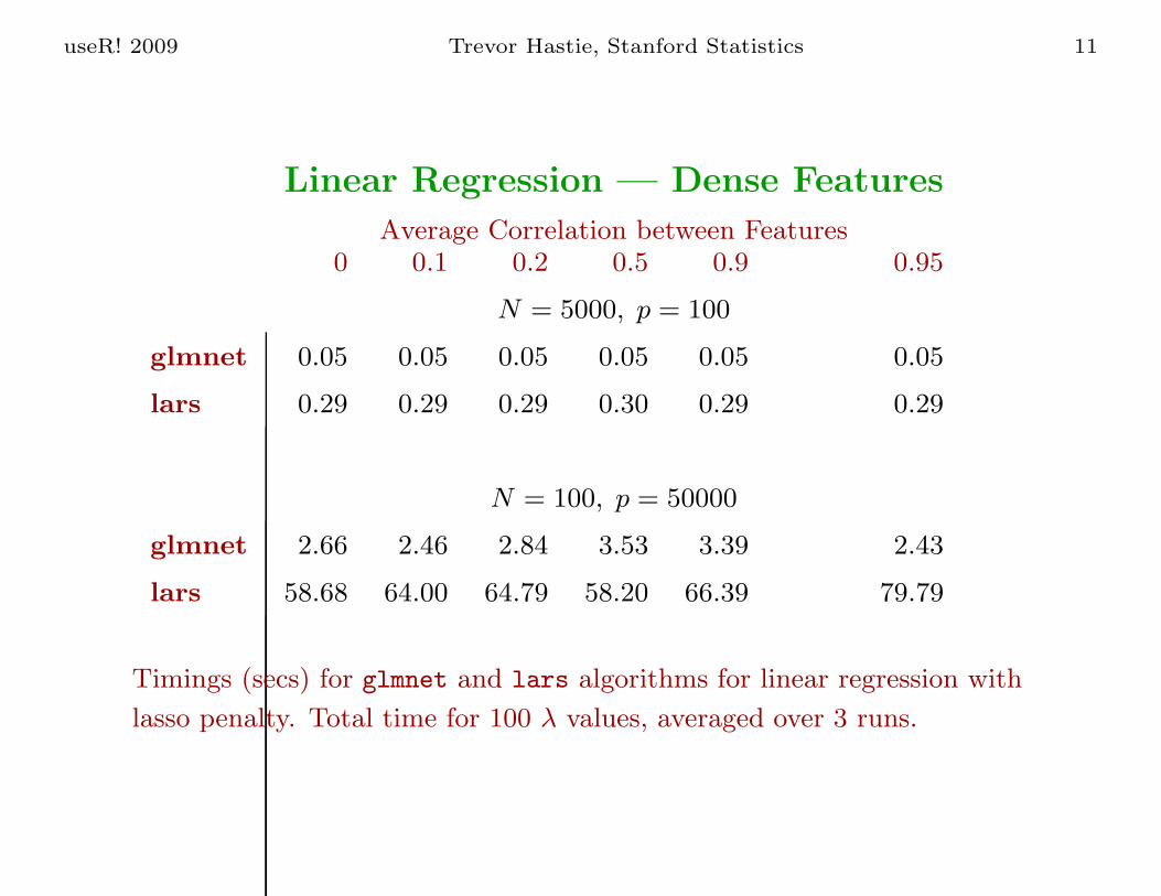
Linear Regression — Dense Features
Average Correlation between Features0 0.1 0.2 0.5 0.9 0.95
N = 5000, p = 100
glmnet 0.05 0.05 0.05 0.05 0.05 0.05
lars 0.29 0.29 0.29 0.30 0.29 0.29
N = 100, p = 50000
glmnet 2.66 2.46 2.84 3.53 3.39 2.43
lars 58.68 64.00 64.79 58.20 66.39 79.79
Timings (secs) for glmnet and lars algorithms for linear regression with
lasso penalty. Total time for 100 λ values, averaged over 3 runs.
useR! 2009 Trevor Hastie, Stanford Statistics 12
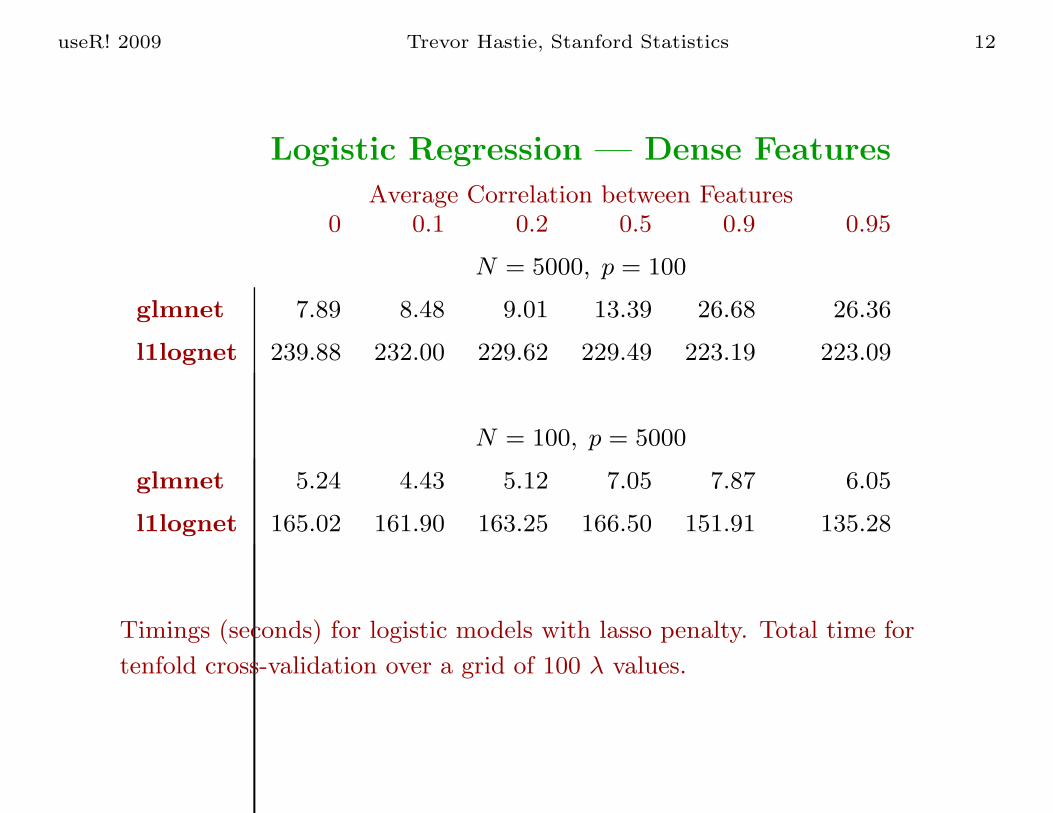
Logistic Regression — Dense Features
Average Correlation between Features0 0.1 0.2 0.5 0.9 0.95
N = 5000, p = 100
glmnet 7.89 8.48 9.01 13.39 26.68 26.36
l1lognet 239.88 232.00 229.62 229.49 223.19 223.09
N = 100, p = 5000
glmnet 5.24 4.43 5.12 7.05 7.87 6.05
l1lognet 165.02 161.90 163.25 166.50 151.91 135.28
Timings (seconds) for logistic models with lasso penalty. Total time for
tenfold cross-validation over a grid of 100 λ values.
useR! 2009 Trevor Hastie, Stanford Statistics 13
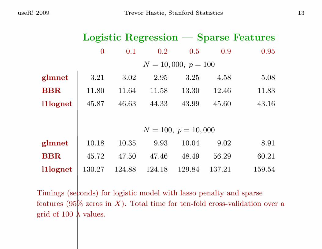
Logistic Regression — Sparse Features
0 0.1 0.2 0.5 0.9 0.95
N = 10, 000, p = 100
glmnet 3.21 3.02 2.95 3.25 4.58 5.08
BBR 11.80 11.64 11.58 13.30 12.46 11.83
l1lognet 45.87 46.63 44.33 43.99 45.60 43.16
N = 100, p = 10, 000
glmnet 10.18 10.35 9.93 10.04 9.02 8.91
BBR 45.72 47.50 47.46 48.49 56.29 60.21
l1lognet 130.27 124.88 124.18 129.84 137.21 159.54
Timings (seconds) for logistic model with lasso penalty and sparse
features (95% zeros in X). Total time for ten-fold cross-validation over a
grid of 100 λ values.
useR! 2009 Trevor Hastie, Stanford Statistics 14
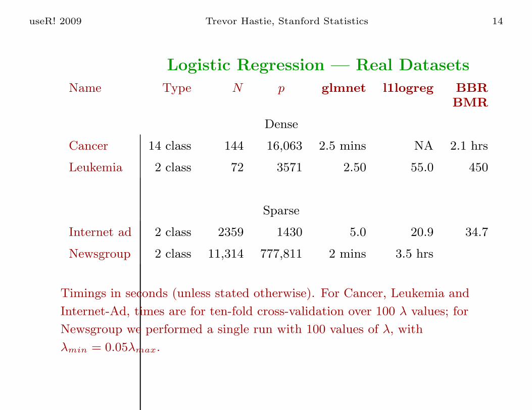
Logistic Regression — Real Datasets
Name Type N p glmnet l1logreg BBRBMR
Dense
Cancer 14 class 144 16,063 2.5 mins NA 2.1 hrs
Leukemia 2 class 72 3571 2.50 55.0 450
Sparse
Internet ad 2 class 2359 1430 5.0 20.9 34.7
Newsgroup 2 class 11,314 777,811 2 mins 3.5 hrs
Timings in seconds (unless stated otherwise). For Cancer, Leukemia and
Internet-Ad, times are for ten-fold cross-validation over 100 λ values; for
Newsgroup we performed a single run with 100 values of λ, with
λmin = 0.05λmax.
useR! 2009 Trevor Hastie, Stanford Statistics 15
A brief history of coordinate descent for the lasso
1997 Tibshirani’s student Wenjiang Fu at U. Toronto develops the“shooting algorithm” for the lasso. Tibshirani doesn’t fullyappreciate it.
.
useR! 2009 Trevor Hastie, Stanford Statistics 16
A brief history of coordinate descent for the lasso
1997 Tibshirani’s student Wenjiang Fu at U. Toronto develops the“shooting algorithm” for the lasso. Tibshirani doesn’t fullyappreciate it.
2002 Ingrid Daubechies gives a talk at Stanford, describes aone-at-a-time algorithm for the lasso. Hastie implements it,makes an error, and Hastie +Tibshirani conclude that themethod doesn’t work.
.
useR! 2009 Trevor Hastie, Stanford Statistics 17
A brief history of coordinate descent for the lasso
1997 Tibshirani’s student Wenjiang Fu at U. Toronto develops the“shooting algorithm” for the lasso. Tibshirani doesn’t fullyappreciate it.
2002 Ingrid Daubechies gives a talk at Stanford, describes aone-at-a-time algorithm for the lasso. Hastie implements it,makes an error, and Hastie +Tibshirani conclude that themethod doesn’t work.
2006 Friedman is external examiner at PhD oral of Anita van derKooij (Leiden) who uses coordinate descent for elastic net.Friedman, Hastie + Tibshirani revisit this problem. Othershave too — Shevade and Keerthi (2003), Krishnapuram andHartemink (2005), Genkin, Lewis and Madigan (2007), Wu andLange (2008), Meier, van de Geer and Buehlmann (2008).
useR! 2009 Trevor Hastie, Stanford Statistics 18
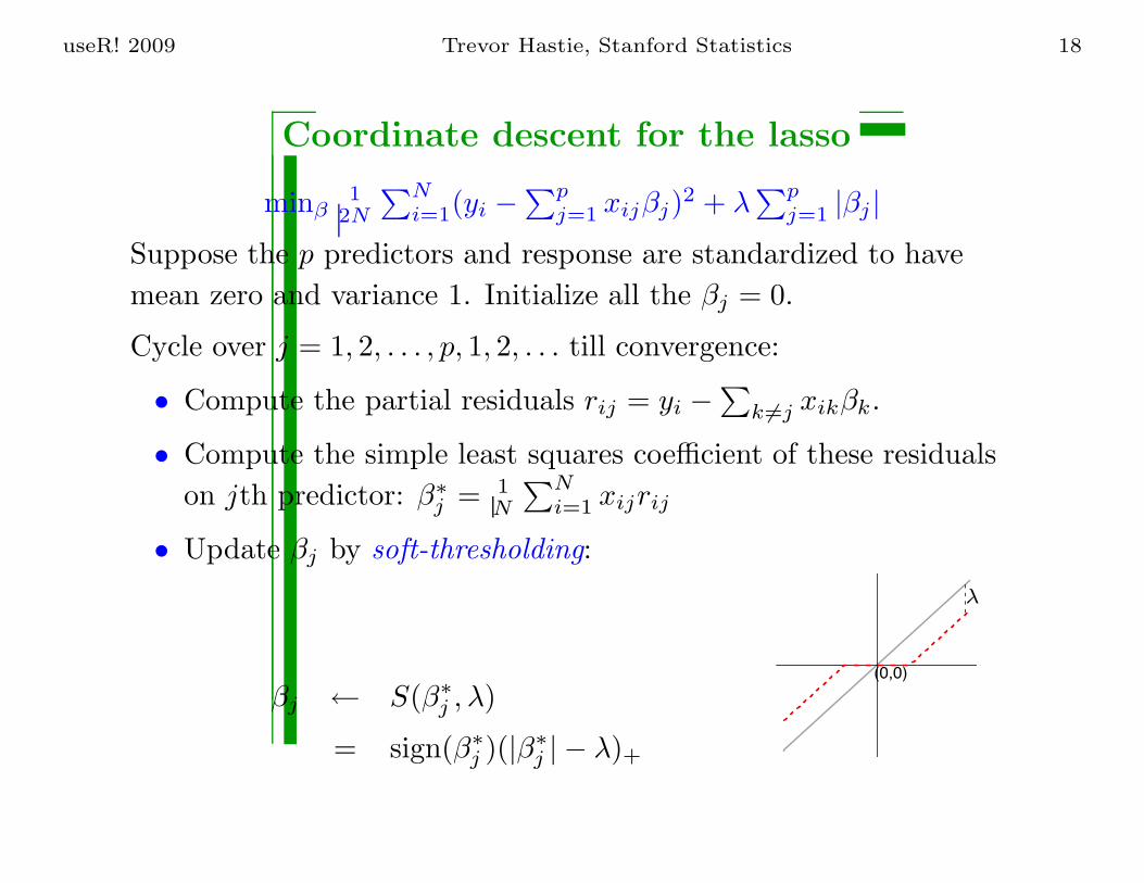
Coordinate descent for the lasso
minβ1
2N
∑Ni=1(yi −
∑pj=1 xijβj)2 + λ
∑pj=1 |βj |
Suppose the p predictors and response are standardized to havemean zero and variance 1. Initialize all the βj = 0.
Cycle over j = 1, 2, . . . , p, 1, 2, . . . till convergence:
• Compute the partial residuals rij = yi −∑
k �=j xikβk.
• Compute the simple least squares coefficient of these residualson jth predictor: β∗
j = 1N
∑Ni=1 xijrij
• Update βj by soft-thresholding:
βj ← S(β∗j , λ)
= sign(β∗j )(|β∗
j | − λ)+
(0,0)
λ
useR! 2009 Trevor Hastie, Stanford Statistics 19
Why is coordinate descent so fast?
There are a number of tricks and strategies that we use exploit thestructure of the problem.
Naive Updates: β∗j = 1
N
∑Ni=1 xijrij = 1
N
∑Ni=1 xijri + βj , where
ri is current model residual; O(N). Many coefficients are zero,and stay zero. If a coefficient changes, residuals are updated inO(N) computations.
Covariance Updates:∑N
i=1 xijri = 〈xj , y〉 −∑
k:|βk|>0〈xj , xk〉βk
Cross-covariance terms are computed once for active variablesand stored (helps a lot when N � p).
Sparse Updates: If data is sparse (many zeros), inner productscan be computed efficiently.
useR! 2009 Trevor Hastie, Stanford Statistics 20
Active Set Convergence: After a cycle through p variables, wecan restrict further iterations to the active set till convergence+ one more cycle through p to check if active set has changed.Helps when p� N .
Warm Starts: We fits a sequence of models from λmax down toλmin = ελmax (on log scale). λmax is smallest value of λ forwhich all coefficients are zero. Solutions don’t change muchfrom one λ to the next. Convergence is often faster for entiresequence than for single solution at small value of λ.
FFT:
.
useR! 2009 Trevor Hastie, Stanford Statistics 21
Active Set Convergence: After a cycle through p variables, wecan restrict further iterations to the active set till convergence+ one more cycle through p to check if active set has changed.Helps when p� N .
Warm Starts: We fits a sequence of models from λmax down toλmin = ελmax (on log scale). λmax is smallest value of λ forwhich all coefficients are zero. Solutions don’t change muchfrom one λ to the next. Convergence is often faster for entiresequence than for single solution at small value of λ.
FFT: Friedman + Fortran + Tricks — no sloppy flops!
.
useR! 2009 Trevor Hastie, Stanford Statistics 22
Binary Logistic Models
Newton Updates: For binary logistic regression we have an outerNewton loop at each λ. This amounts to fitting a lasso withweighted squared error-loss. Uses weighted soft thresholding.
Multinomial: We use a symmetric formulation for multi- classlogistic:
Pr(G = �|x) =eβ0�+xT β�
∑Kk=1 eβ0k+xT βk
.
This creates an additional loop, as we cycle through classes,and compute the quadratic approximation to the multinomiallog-likelihood, holding all but one class’s parameters fixed.
Details Many important but tedious details with logistic models.e.g. if p� N , cannot let λ run down to zero.
useR! 2009 Trevor Hastie, Stanford Statistics 23
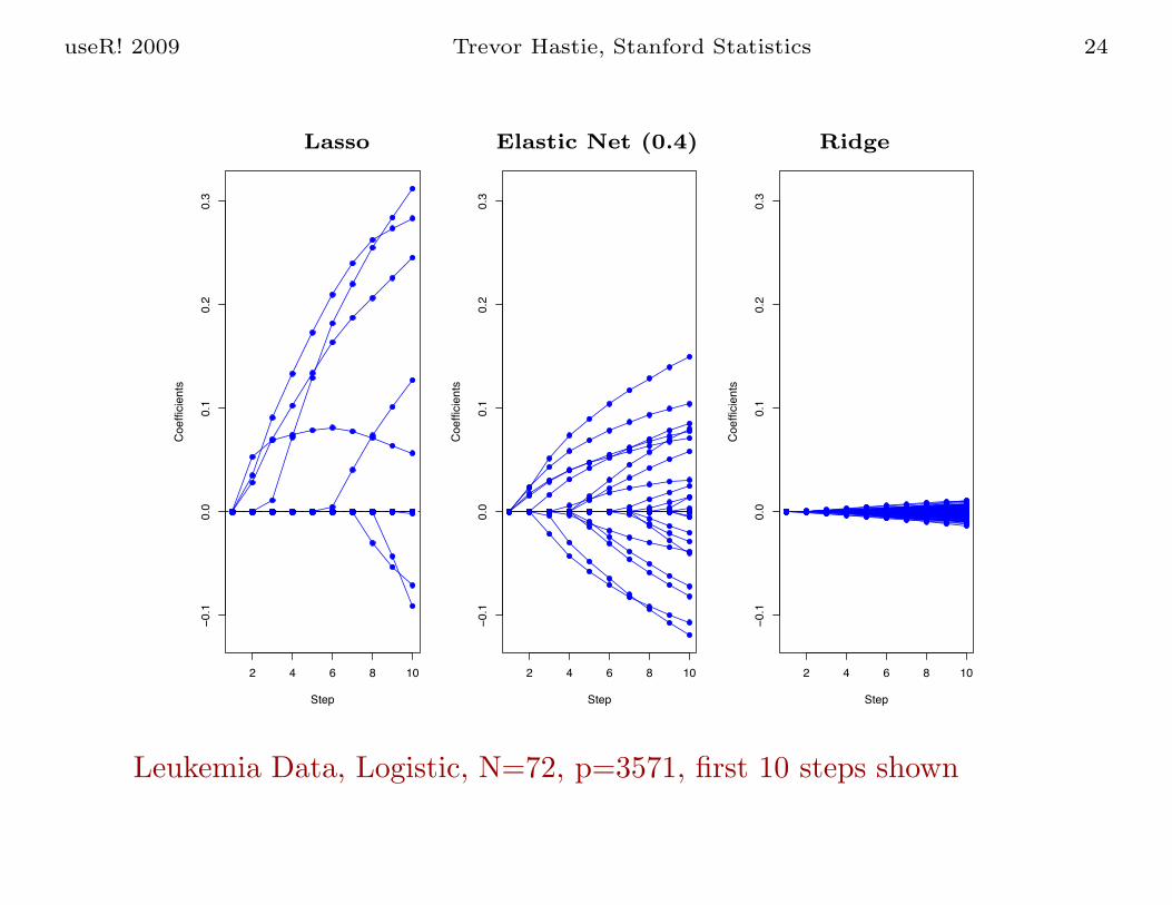
Elastic-net Penalty
Proposed in Zou and Hastie (2005) for p� N situations, wherepredictors are correlated in groups.
Pα(β) =p∑
j=1
[12 (1− α)β2
j + α|βj |].
α creates a compromise between the lasso and ridge.
Coordinate update is now
βj ←S(β∗
j , λα)1 + λ(1− α)
where β∗j = 1
N
∑Ni=1 xijrij as before.
useR! 2009 Trevor Hastie, Stanford Statistics 24
2 4 6 8 10
−0.
10.
00.
10.
20.
3
Step
Coe
ffici
ents
2 4 6 8 10
−0.
10.
00.
10.
20.
3
Step
Coe
ffici
ents
2 4 6 8 10
−0.
10.
00.
10.
20.
3
Step
Coe
ffici
ents
Lasso Elastic Net (0.4) Ridge
Leukemia Data, Logistic, N=72, p=3571, first 10 steps shown
useR! 2009 Trevor Hastie, Stanford Statistics 25
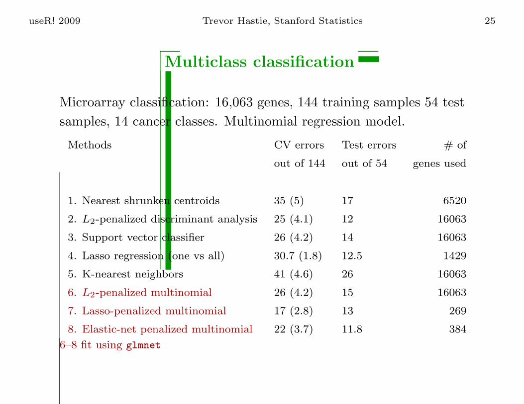
Multiclass classification
Microarray classification: 16,063 genes, 144 training samples 54 testsamples, 14 cancer classes. Multinomial regression model.
Methods CV errors Test errors # of
out of 144 out of 54 genes used
1. Nearest shrunken centroids 35 (5) 17 6520
2. L2-penalized discriminant analysis 25 (4.1) 12 16063
3. Support vector classifier 26 (4.2) 14 16063
4. Lasso regression (one vs all) 30.7 (1.8) 12.5 1429
5. K-nearest neighbors 41 (4.6) 26 16063
6. L2-penalized multinomial 26 (4.2) 15 16063
7. Lasso-penalized multinomial 17 (2.8) 13 269
8. Elastic-net penalized multinomial 22 (3.7) 11.8 384
6–8 fit using glmnet
useR! 2009 Trevor Hastie, Stanford Statistics 26
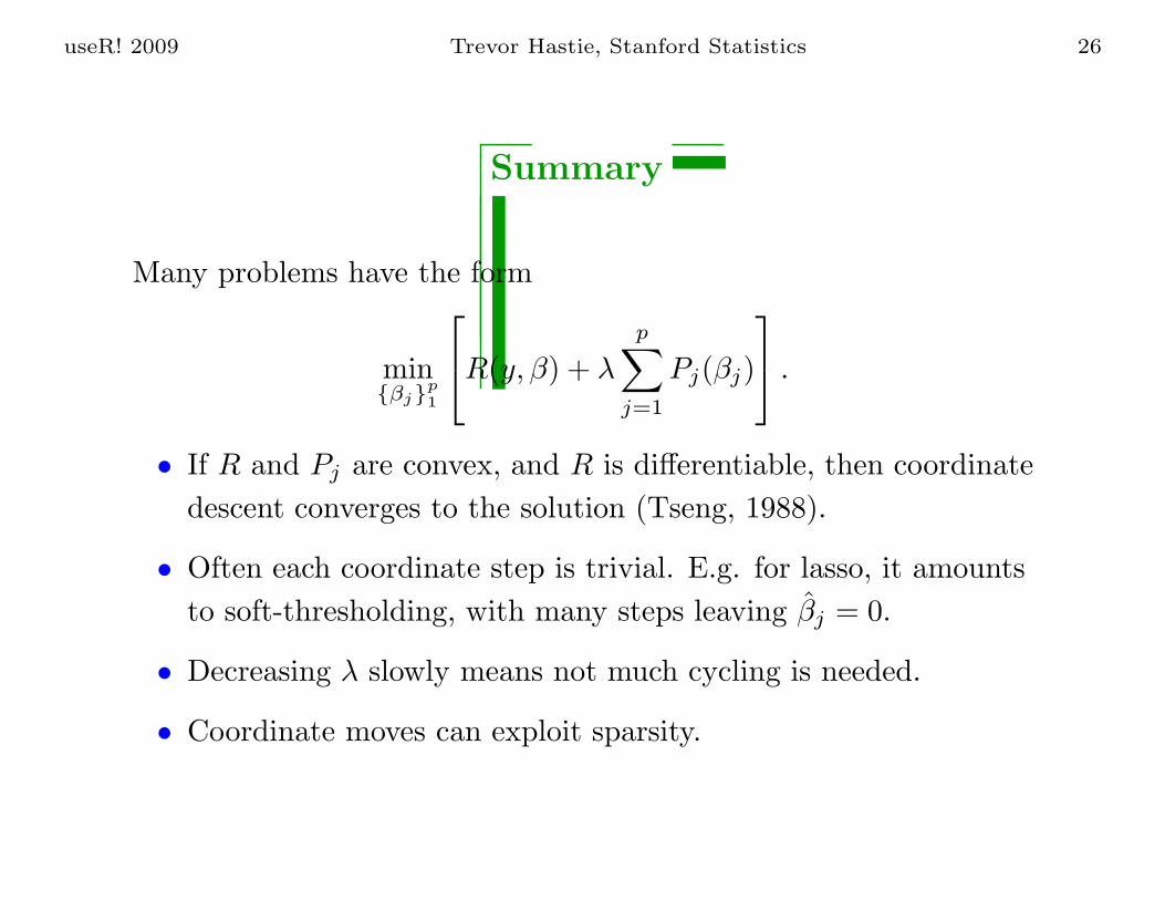
Summary
Many problems have the form
min{βj}p
1
⎡⎣R(y, β) + λ
p∑j=1
Pj(βj)
⎤⎦ .
• If R and Pj are convex, and R is differentiable, then coordinatedescent converges to the solution (Tseng, 1988).
• Often each coordinate step is trivial. E.g. for lasso, it amountsto soft-thresholding, with many steps leaving β̂j = 0.
• Decreasing λ slowly means not much cycling is needed.
• Coordinate moves can exploit sparsity.
useR! 2009 Trevor Hastie, Stanford Statistics 27
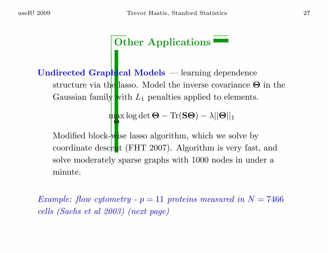
Other Applications
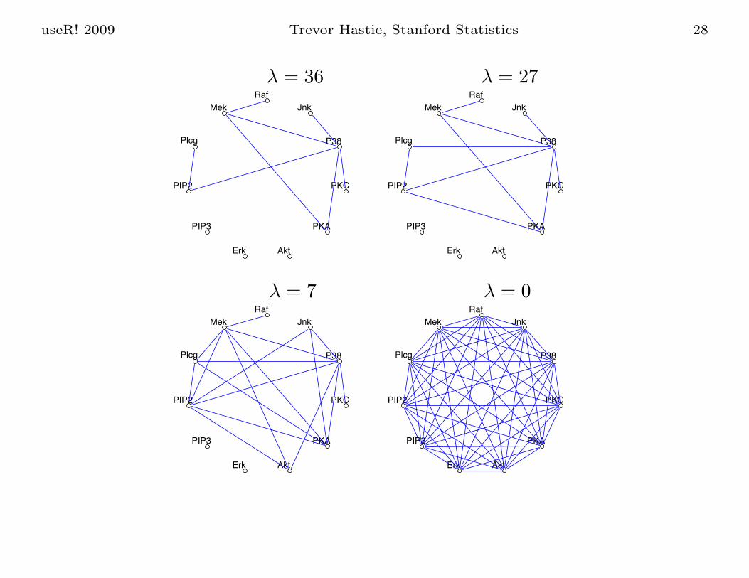
Undirected Graphical Models — learning dependencestructure via the lasso. Model the inverse covariance Θ in theGaussian family with L1 penalties applied to elements.
maxΘ
log detΘ− Tr(SΘ)− λ||Θ||1
Modified block-wise lasso algorithm, which we solve bycoordinate descent (FHT 2007). Algorithm is very fast, andsolve moderately sparse graphs with 1000 nodes in under aminute.
Example: flow cytometry - p = 11 proteins measured in N = 7466cells (Sachs et al 2003) (next page)
useR! 2009 Trevor Hastie, Stanford Statistics 28
RafMek
Plcg
PIP2
PIP3
Erk Akt
PKA
PKC
P38
JnkRaf
Mek
Plcg
PIP2
PIP3
Erk Akt
PKA
PKC
P38
Jnk
RafMek
Plcg
PIP2
PIP3
Erk Akt
PKA
PKC
P38
JnkRaf
Mek
Plcg
PIP2
PIP3
Erk Akt
PKA
PKC
P38
Jnk
λ = 0λ = 7
λ = 27λ = 36
useR! 2009 Trevor Hastie, Stanford Statistics 29
Grouped lasso (Yuan and Lin, 2007, Meier, Van de Geer,Buehlmann, 2008) — each term Pj(βj) applies to sets ofparameters:
J∑j=1
||βj ||2.
Example: each block represents the levels for a categoricalpredictor.Leads to a block-updating form of coordinate descent.
useR! 2009 Trevor Hastie, Stanford Statistics 30
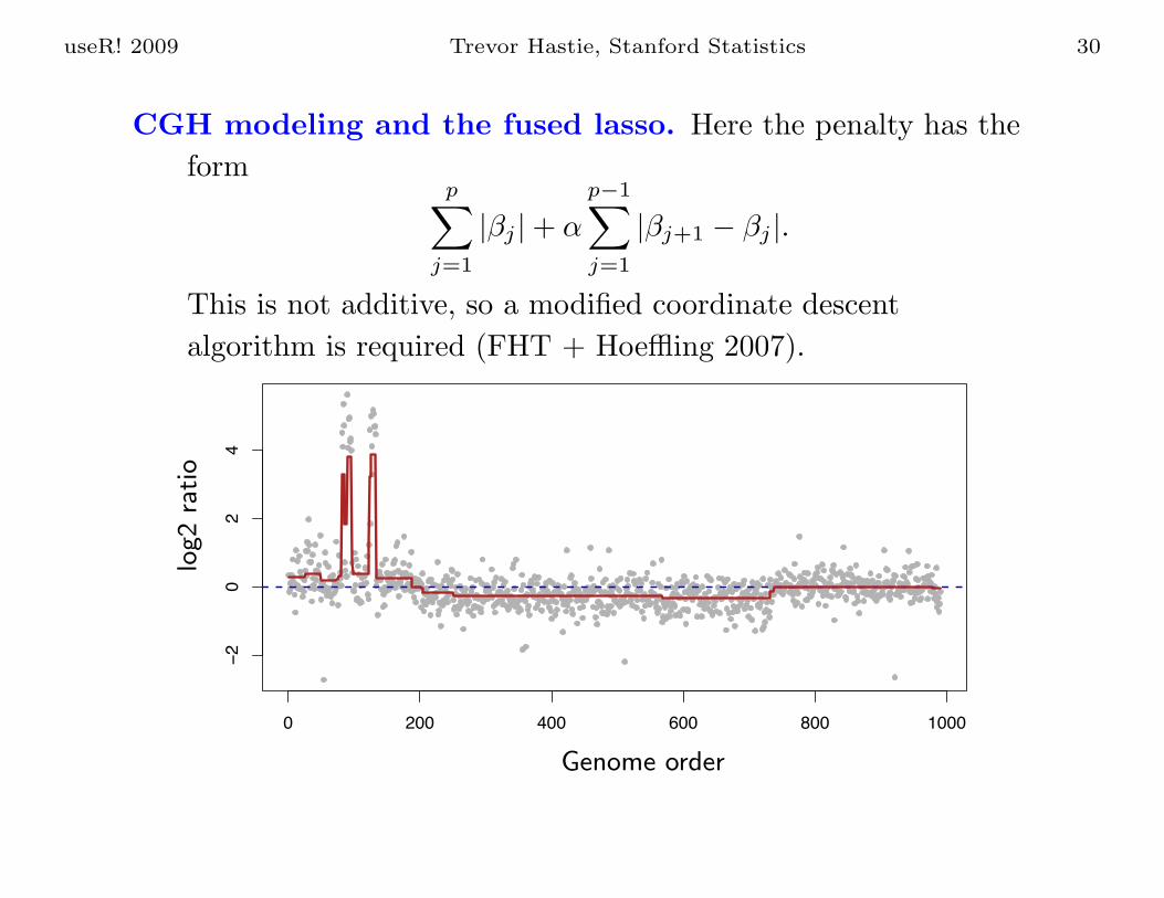
CGH modeling and the fused lasso. Here the penalty has theform
p∑j=1
|βj |+ α
p−1∑j=1
|βj+1 − βj |.
This is not additive, so a modified coordinate descentalgorithm is required (FHT + Hoeffling 2007).
0 200 400 600 800 1000
−2
02
4
Genome order
log2
ratio
useR! 2009 Trevor Hastie, Stanford Statistics 31
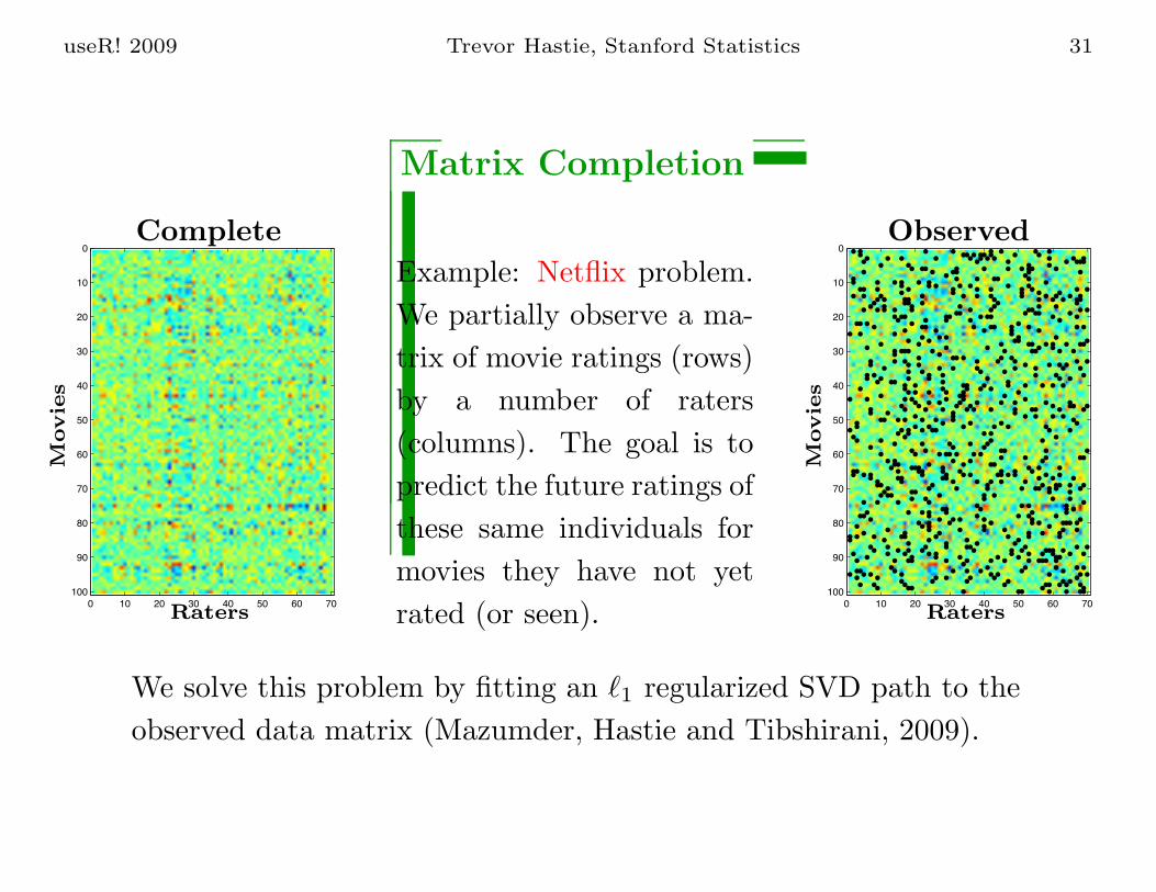
Matrix Completion
0 10 20 30 40 50 60 70
0
10
20
30
40
50
60
70
80
90
100
Complete
Movie
s
Raters
Example: Netflix problem.We partially observe a ma-trix of movie ratings (rows)by a number of raters(columns). The goal is topredict the future ratings ofthese same individuals formovies they have not yetrated (or seen). 0 10 20 30 40 50 60 70
0
10
20
30
40
50
60
70
80
90
100
Observed
Movie
s
Raters
We solve this problem by fitting an �1 regularized SVD path to theobserved data matrix (Mazumder, Hastie and Tibshirani, 2009).
useR! 2009 Trevor Hastie, Stanford Statistics 32
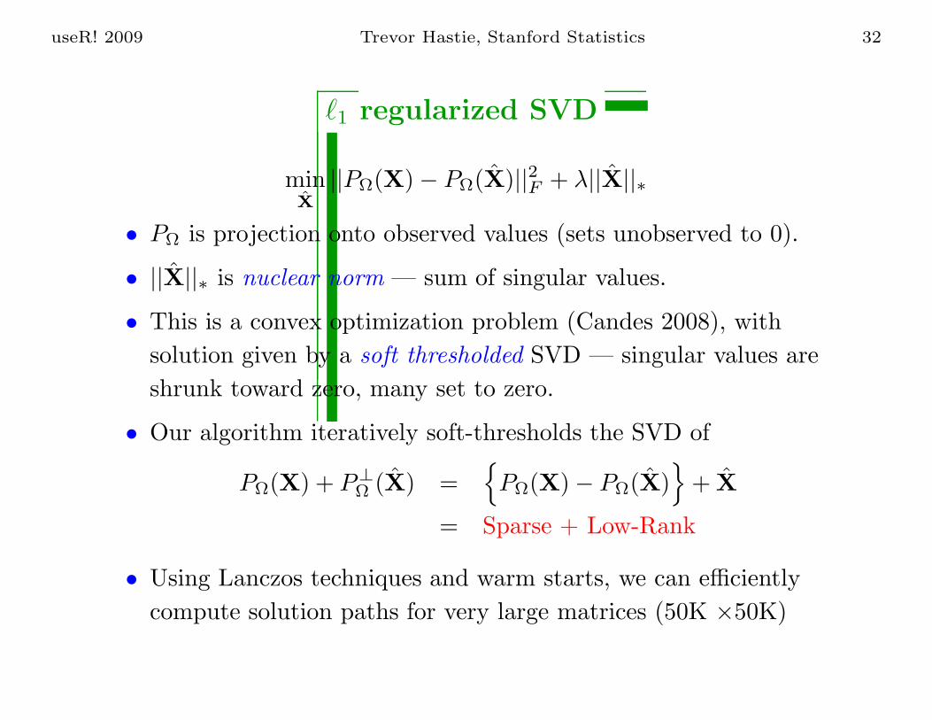
�1 regularized SVD
minX̂||PΩ(X)− PΩ(X̂)||2F + λ||X̂||∗
• PΩ is projection onto observed values (sets unobserved to 0).
• ||X̂||∗ is nuclear norm — sum of singular values.
• This is a convex optimization problem (Candes 2008), withsolution given by a soft thresholded SVD — singular values areshrunk toward zero, many set to zero.
• Our algorithm iteratively soft-thresholds the SVD of
PΩ(X) + P⊥Ω (X̂) =
{PΩ(X)− PΩ(X̂)
}+ X̂
= Sparse + Low-Rank
• Using Lanczos techniques and warm starts, we can efficientlycompute solution paths for very large matrices (50K ×50K)
useR! 2009 Trevor Hastie, Stanford Statistics 33
Summary
• �1 regularization (and variants) has become a powerful toolwith the advent of wide data.
• In compressed sensing, often exact sparse signal recovery ispossible with �1 methods.
• Coordinate descent is fastest known algorithm for solving theseproblems—along a path of values for the tuning parameter.