Fast Simulation of Gaussian-Mode Scattering for Precision Interferometry

D. Brown,1, ∗ R. J. E. Smith,2 and A. Freise1

1University of Birmingham, Edgbaston, B15 2TT, UK2LIGO, California Institute of Technology, Pasadena, CA 91125, USA

Understanding how laser light scatters from realistic mirror surfaces is crucial for the design, com-missioning and operation of precision interferometers, such as the current and next generation ofgravitational-wave detectors. Numerical simulations are indispensable tools for this task but theirutility can in practice be limited by the computational cost of describing the scattering process.In this paper we present an efficient method to significantly reduce the computational cost of op-tical simulations that incorporate scattering. This is accomplished by constructing a near optimalrepresentation of the complex, multi-parameter 2D overlap integrals that describe the scatteringprocess (referred to as a reduced order quadrature). We demonstrate our technique by simulating anear-unstable Fabry-Perot cavity and its control signals using similar optics to those installed in oneof the LIGO gravitational-wave detectors. We show that using reduced order quadrature reducesthe computational time of the numerical simulation from days to minutes (a speed-up of ≈ 2750×)whilst incurring negligible errors. This significantly increases the feasibility of modelling interfer-ometers with realistic imperfections to overcome current limits in state-of-the-art optical systems.Whilst we focus on the Hermite-Gaussian basis for describing the scattering of the optical fields, ourmethod is generic and could be applied with any suitable basis. An implementation of this reducedorder quadrature method is provided in the open source interferometer simulation software Finesse.

I. INTRODUCTION

Laser interferometers have long been an exceptionaltool for enabling high precision measurements. Withever increasing demands on their performance, new tech-niques and tools have been developed to design and buildthe next-generation of instruments. This has especiallybeen true in the development of gravitational-wave de-tectors over the last several decades [1–4]. Such ground-based gravitational-wave detectors are based on a Michel-son interferometer and are enhanced with Fabry-Perotcavities. Detecting gravitational waves is still one of themajor challenges in experimental physics, and the inter-ferometers used include numerous new optical technolo-gies to reach unprecedented displacement sensitivities be-yond 10−19 m/

√Hz.

Some of these detectors are currently being upgradedto have a ten-fold increase in sensitivity using a muchhigher circulating power [5, 6]. To achieve their targetperformance the detectors undergo several years of com-missioning, during which the interferometers are carefullytested and improved towards their designed operationalstate. Numerical simulations are important tools to di-agnose causes of any unexpected behaviour seen duringcommissioning; to suggest solutions to potential prob-lems and for advising the design of detector upgrades.Hence, there is a long history of developing and usingdedicated optical simulation tools for the commissioningand design of gravitational-wave detectors [7–10].

One of the key aspects for the current instruments isthe high circulating laser power, up to hundreds of kilo-Watts, required for a broadband reduction of shot-noise.

∗ Corresponding author: ddb@star.sr.bham.ac.uk

It has been recognised for some time that the thermaldeformations of the optics due to spurious absorptioncan degrade the performance of the interferometers [11].Numerical models have been used extensively in the in-vestigation of such problems and in the development ofmitigating solutions (for example [12, 13]). Thermallyinduced distortions and other effects related to the laserbeam shape are still limiting factors of the instrumentstoday and are concerns for the design of future detec-tors [14]. Furthermore, similar effects can limit the per-formance of other optical precision measurements suchas optical clocks [15] or the optical readout of atomicsystems [16]. Mitigation strategies for beam shape dis-tortions in complex interferometers are actively being de-veloped and require accurate numerical models for theirdesign and development.

Initially, the simulation tools for investigating dis-torted beams used a grid-based field description. Beamdistortions can also be modeled effectively using an ex-pansion into spatial cavity eigenmodes [17], such asHermite-Gauss modes. The interaction of the beamshape with a distorted optical surface often requires thecomputation of a scattering matrix based on measured orsimulated profiles of the distorted surface. This is alwaystrue for mode-based simulations programs but is also re-quired for grid-based codes when specific shapes of thebeam are important, for example, for the investigationsof parametric instabilities [? ? ]. If this matrix has to bere-generated, for example when the effects of a change ofa surface shape is being investigated, this element of thecomputation can dominate the total time required for theentire simulation. A prominent example is that when thecirculating laser power within the LIGO interferometersthermally warps the mirror surfaces changing the shapeof the laser beams and requiring a re-calculation of manyscattering matrices. Including this effect can increase the

arX

iv:1

507.

0380

6v2

[ph

ysic

s.op

tics]

13

Aug

201

5

2

computation time from minutes to days.

Some of us are providing numerical simulation supportfor the commissioning of the LIGO interferometers [18].We use our own simulation tool Finesse [19] and aremaintaining parameter files for the detectors [20]. Com-missioning tackles the unexpected behaviour of the in-terferometers and must take into account the sometimesrapid progress of the experimental setup. Therefore sup-port provided with numerical models must fulfil two cri-teria: a) we must be able to accurately model the currentexperimental setup in the presence of distortions and de-viations from the design and b) we must be able to pro-vide a quick response to new questions to inform themanagement of the activities on site in real time. Fi-nesse is a frequency-domain tool, using Hermite-Gaussmodes to describe beam distortions and is thus ideallysuited as a rapid and accurate tool.

Our investigations with numerical tools typically con-sist of a sequence of different subtasks, sometimes usingdifferent tools, alternating with an expert review of in-termediate or preliminary results. This is a very differentpattern of tasks to those that benefit from a computercluster or super computer. Instead, our work requireslightweight and flexible tools with computing times upto minutes or hours. Because of this, strategies to ame-liorate the run time of simulations are of high importanceto provide fast diagnosis of unexpected behaviour; to al-low the parameter space of the simulations to be probedexhaustively; to improve the resolution of simulations ata fixed run-time, and to allow simulations to be run onless powerful and cheaper hardware.

In this paper we present a new approach that reducesthe computational time of simulations based on modalmodels by several orders of magnitude. We specificallytarget the computational cost of computing scatteringmatrices for optical simulations. Our approach is basedon a near-optimal formulation of the integrals requiredto compute the scattering matrices, known as a reducedorder quadrature [21] (ROQ). The reduced order quadra-ture has already been applied in the context of astro-nomical data analysis with LIGO [22] where the repeatedcomputation of quantities similar to the scattering matrixdominate the run time of the analysis codes. Crucially,the reduced order quadrature is designed to provide hugeimprovements to computational efficiency whilst main-taining computational precision.

The ROQ can be regarded as a type of near-optimal,application specific, downsampling of the integrandsneeded to compute the integrals for the scattering ma-trices [21]. It is analogous to Gaussian quadrature, butwhereas Gaussian quadrature is designed to provide ex-act results for polynomials of a certain degree, the ROQproduces nearly-exact results for arbitrary parametricfunctions. Importantly, we are able to place tight er-ror bounds on the accuracy of the ROQ for a particularapplication [21] making it an ideal technique to speed upcostly integrals. It exploits an offline/online methodol-ogy in which we recast the expensive integrals used to

compute scattering matrices into a more computation-ally efficient form in the “offline” stage. This is thenused for the rapid “online” evaluation of the scatteringmatrices. The offline stage can itself be computationallyexpensive, however it need only be performed once andis easily parallelised. The data computed in the offlinestage—that is needed by the ROQ—can be stored andshared for particular use cases in the online stage so thatthe offline cost does not need to be factored in at runtime.

We derive the algorithm in a general form and reporton the implementation and performance of this methodin an example task for the LIGO interferometers. Theimplementation of the method described in this article isavailable as open source as part of the Finesse sourcecode and the Python based package Pykat [? ], whichwill also contain the offline computed data to enable oth-ers to model Advanced LIGO like arm cavities. Our par-ticular implementation here is used to provide a simple,real-word example. However, the algorithm can be eas-ily implemented in other types of simulation tools, forexample, time domain simulations or grid based tools(also known as FFT simulations) that compare beamshapes. In all cases our algorithm can significantly reducethe computation time for evaluating overlap integrals ofGaussian modes with numerical data.

The paper is outlined as follows: In section II we givean overview of the paraxial description of the opticaleigenmodes and scattering into higher order modes. InSection III we provide the mathematical background andalgorithm for producing the ROQ. Section III heavily re-lies on an additional mathematical technique known asthe “empirical interpolation method” [23]. We assumeno prior knowledge of this and provide the main detailsand results necessary for the ROQ. Section IV then high-lights an exemplary case to demonstrate our method formodelling near-unstable optical cavities. Finally in sec-tion V the computational performance of our method isanalysed.

II. HIGHER-ORDER OPTICAL MODES

Gravitational wave detectors are constructed of multi-ple optical cavities based on a Michelson interferometer.The circulating laser beams in such an optical setup iswell described by the the paraxial Gaussian eigenmodesof a spherical cavity; an efficient basis for describing thespatial properties of a laser beam in the transverse planeto the propagation axis [24]. The fundamental Gaussianmode is described in cartesian coordinates by:

u00(x, y; qx, qy) =

√2

πwx(qx)wy(qy)e−ik

(x2

2qx+ y2

2qy

)(1)

wx and wy are the beam spot sizes in the x and y di-rections, k is the wavenumber of the laser light andq = {qx, qy} are the complex beam parameters in the

3

x and y directions. The shape of the Gaussian mode isfully defined by the wavelength of the light λ and thebeam parameter:

qx = zx + izR,x = zx + iπw2

0,x

λ(2)

where zx is the distance from the waist, zR,x is theRayleigh range, w0,x is the size of the waist and λ =1064nm is the wavelength of the Nd:YAG laser used incurrent GW detectors. The same set of parameters existsfor qy.

Any perturbations in the beam’s spatial profile fromthis fundamental Gaussian can be described by the ad-dition of higher-order Gaussian modes (HOMs). In thispaper we discuss in particular the cartesian orthogonalbasis of Hermite-Gaussian (HG) modes [24], however ourmethod is applicable for any other suitable basis. Thecomplex transverse spatial amplitude of these HG modesis given by:

unm(x, y, qx, qy) = un(x, qx)um(y, qy)

un(x, q) =

(2

π

)1/4(1

2nn!w0

)1/2(q0q

)1/2

(q0 q

∗

q∗0 q

)n/2Hn

(√2x

w(z)

)exp

(−ikx2

2q

). (3)

where n defines the order of the Hermite polynomials Hn

in the x axis and m for the y. The order of the opticalmode is O = n + m and individual modes are typicallyreferred to as TEMnm. A laser field with a single opticalfrequency component ω can be expanded into a beambasis whose shape is described by q as:

E(x, y, t;q) =

n+m≤Omax∑n=0,m=0

anmunm(x, y;q)eiωt (4)

where anm is a complex value describing the amplitudeand phase of a mode TEMnm and Omax is the maximumorder of modes included in the expansion.

A. Scattering into higher-order modes

When a field interacts with an optical component itsmode content is typically changed. Here we define scat-tering as the relationship between the mode content ofthe outgoing beams a with a beam shape q, and themode content of the incoming beam a′ described with

q′. Mathematically this is simply a = ka′ where k isknown as the scattering matrix. Now consider the spa-tial profile of a beam reflected from on an imperfect opticE′(x, y;q′) = A(x, y)Ein(x, y;q′), where Ein is the inci-dent beam and A(x, y) is complex function describing theperturbation it has undergone. For example, on reflec-tion a beam will be clipped by the finite size of the mirrorα(x, y) and reflected from a surface with height variations

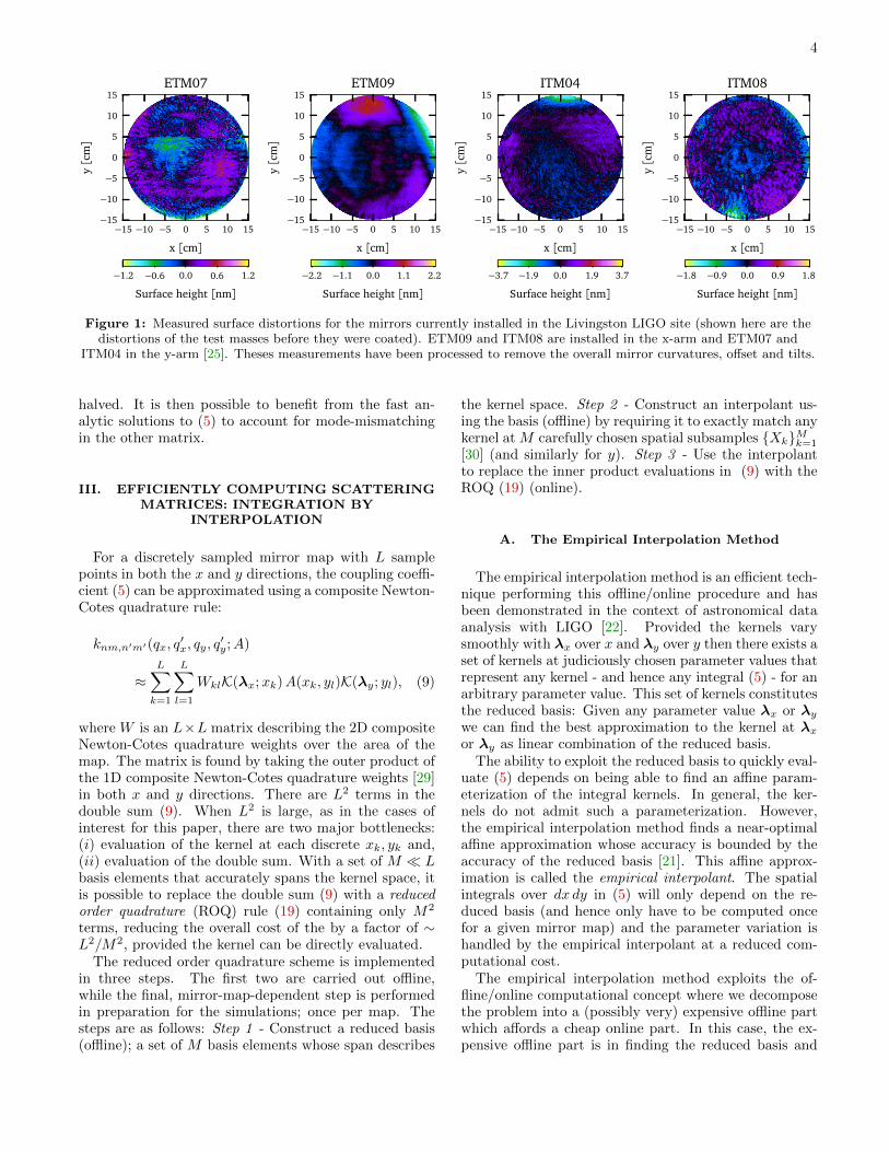
z(x, y). Thus, both the amplitude and phase of the beamwill be affected and A(x, y) = α(x, y)ei2k z(x,y). An exam-ple of the measured surface height variations present onLIGO test mass mirrors can be seen in figure 1 [25]. Themode content of the outgoing beam E(x, y;q) is com-puted by projecting E′ into the outgoing beam basis q.For any incoming HOM un′m′ the amount of outgoingunm can be computed via an overlap integral, this com-plex value is known as a coupling coefficient :

knm,n′m′(qx, q′x, qy, q

′y;A) =∫∫ ∞

−∞K(λx;x)A(x, y)K(λy; y) dx dy , (5)

where the integral kernels K(λx;x) and K(λy; y) aregiven by

K(λx;x) = u∗n(x, qx)un′(x, q′x) , (6)

K(λy; y) = u∗m(y, qy)um′(y, q′y) , (7)

and the parameter vectors are given by λx =(n, n′, qx, q

′x) and λy = (m,m′, qy, q

′y). There are two

general cases when computing (5): q 6= q′ which we referto as mode-mismatched and q = q′ as mode-matched.

Computing the scattering matrix k requires evaluat-ing the integral (5) for each of its elements. If couplingsbetween modes up to and including order O are con-

sidered then the number of elements in k is Nk(O) =(O4 + 6O3 + 13O2 + 12O + 4)/4 and the computationalcost of evaluating this many integrals can be very expen-sive. In our experience [18, 26] a typical LIGO simulationtask involving HOMs can be performed with O = 6− 10while some cases, such as those that include strong ther-mal distortions or clipping, a higher maximum order isrequired.

In simple cases where A(x, y) = 1 or A(x, y) repre-sents a tilted surface, analytical results are available forboth mode matched and mismatched cases [27, 28]. Ingeneral however A(x, y) is of no particular form and theintegral in (5) must be evaluated numerically. It is pos-sible to split multiple distortions into separate scatteringmatrices A(x, y) ⇒ A(x, y)B(x, y) and the coupling co-efficients become a product of two separate matrices:

knm,n′m′(q,q′;AB) =

∞∑n,m=0

knm,nm(q, q;A) knm,n′m′(q,q′;B) (8)

where q is an expansion beam parameter which we arefree to choose. Thus our scattering matrix becomes

k(q,q′) = kA(q, q)kB(q,q′). By choosing q = q or q′

we can set the mode-mismatching to be in either one ma-

trix or the other. This is ideal as a mode-matched k isa Hermitian matrix whose symmetry can be exploited toonly compute one half of the matrix. By ensuring thatthis matrix also contains any distortions that require nu-merical integration the computational cost can be nearly

4

−15 −10 −5 0 5 10 15

x [cm]

−15

−10

−5

0

5

10

15y[c

m]

ETM07

−1.2 −0.6 0.0 0.6 1.2

Surface height [nm]

−15 −10 −5 0 5 10 15

x [cm]

−15

−10

−5

0

5

10

15

y[c

m]

ETM09

−2.2 −1.1 0.0 1.1 2.2

Surface height [nm]

−15 −10 −5 0 5 10 15

x [cm]

−15

−10

−5

0

5

10

15

y[c

m]

ITM04

−3.7 −1.9 0.0 1.9 3.7

Surface height [nm]

−15 −10 −5 0 5 10 15

x [cm]

−15

−10

−5

0

5

10

15

y[c

m]

ITM08

−1.8 −0.9 0.0 0.9 1.8

Surface height [nm]

Figure 1: Measured surface distortions for the mirrors currently installed in the Livingston LIGO site (shown here are thedistortions of the test masses before they were coated). ETM09 and ITM08 are installed in the x-arm and ETM07 and

ITM04 in the y-arm [25]. Theses measurements have been processed to remove the overall mirror curvatures, offset and tilts.

halved. It is then possible to benefit from the fast an-alytic solutions to (5) to account for mode-mismatchingin the other matrix.

III. EFFICIENTLY COMPUTING SCATTERINGMATRICES: INTEGRATION BY

INTERPOLATION

For a discretely sampled mirror map with L samplepoints in both the x and y directions, the coupling coeffi-cient (5) can be approximated using a composite Newton-Cotes quadrature rule:

knm,n′m′(qx, q′x, qy, q

′y;A)

≈L∑k=1

L∑l=1

WklK(λx;xk)A(xk, yl)K(λy; yl), (9)

where W is an L×L matrix describing the 2D compositeNewton-Cotes quadrature weights over the area of themap. The matrix is found by taking the outer product ofthe 1D composite Newton-Cotes quadrature weights [29]in both x and y directions. There are L2 terms in thedouble sum (9). When L2 is large, as in the cases ofinterest for this paper, there are two major bottlenecks:(i) evaluation of the kernel at each discrete xk, yk and,(ii) evaluation of the double sum. With a set of M � Lbasis elements that accurately spans the kernel space, itis possible to replace the double sum (9) with a reducedorder quadrature (ROQ) rule (19) containing only M2

terms, reducing the overall cost of the by a factor of ∼L2/M2, provided the kernel can be directly evaluated.

The reduced order quadrature scheme is implementedin three steps. The first two are carried out offline,while the final, mirror-map-dependent step is performedin preparation for the simulations; once per map. Thesteps are as follows: Step 1 - Construct a reduced basis(offline); a set of M basis elements whose span describes

the kernel space. Step 2 - Construct an interpolant us-ing the basis (offline) by requiring it to exactly match anykernel at M carefully chosen spatial subsamples {Xk}Mk=1[30] (and similarly for y). Step 3 - Use the interpolantto replace the inner product evaluations in (9) with theROQ (19) (online).

A. The Empirical Interpolation Method

The empirical interpolation method is an efficient tech-nique performing this offline/online procedure and hasbeen demonstrated in the context of astronomical dataanalysis with LIGO [22]. Provided the kernels varysmoothly with λx over x and λy over y then there exists aset of kernels at judiciously chosen parameter values thatrepresent any kernel - and hence any integral (5) - for anarbitrary parameter value. This set of kernels constitutesthe reduced basis: Given any parameter value λx or λywe can find the best approximation to the kernel at λxor λy as linear combination of the reduced basis.

The ability to exploit the reduced basis to quickly eval-uate (5) depends on being able to find an affine param-eterization of the integral kernels. In general, the ker-nels do not admit such a parameterization. However,the empirical interpolation method finds a near-optimalaffine approximation whose accuracy is bounded by theaccuracy of the reduced basis [21]. This affine approx-imation is called the empirical interpolant. The spatialintegrals over dx dy in (5) will only depend on the re-duced basis (and hence only have to be computed oncefor a given mirror map) and the parameter variation ishandled by the empirical interpolant at a reduced com-putational cost.

The empirical interpolation method exploits the of-fline/online computational concept where we decomposethe problem into a (possibly very) expensive offline partwhich affords a cheap online part. In this case, the ex-pensive offline part is in finding the reduced basis and

5

constructing the empirical interpolant. Once the empiri-cal interpolant is found then we use it for the fast onlineevaluation of (5). One of the main reasons why the em-pirical interpolant is used for fast online evaluation of(5) is due to its desirable error properties that makes itsuperior to other interpolation methods, such as polyno-mial interpolation. In addition, the empirical interpolantavoids many of the pitfalls of high-dimensional interpo-lation that we would otherwise encounter (see, e.g. [31]).

B. Affine Parameterization

We would like the kernel to be separable in the modeparameters (λx,λy) and spatial position (x, y). For thesereasons we will look for a representation of the kernel thathas the following form:

K(λx;x) = a(λx) f(x) ,

K(λy; y) = a(λy) f(y) . (10)

The functions a and f are the same irrespective ofwhether the kernel is a function of x or y due to the sym-metries of the Hermite Gauss modes. Using the affineparameterization, the coupling coefficient (5) is:

knm,n′m′(qx, q′x, qy, q

′y) = a∗(λx)a(λy)∫∫ ∞−∞

f∗(x)A(x, y)f(y)dx dy , (11)

This affine parameterization thus allows us to compute allthe parameter-dependent pieces efficiently in the onlineprocedure as all the x − y integrals are performed onlyonce for a given mirror map. In general the kernel willnot admit an exact affine decomposition as in (10). Usingthe EIM, the approximation to the kernels will have theform:

K(λx;x) ≈∑i

ci(λx) ei(x) , (12)

K(λy; y) ≈∑i

ci(λy) ei(y) .

The sum is over the reduced basis elements ei and coef-ficients ci that contain the parameter dependence.

Given a basis ei(x), the ci(λx) in (12) are the solu-tions to the M-point interpolation problem whereby werequire the interpolant to be exactly equal to the kernelat any parameter value λx at a set of interpolation nodes{X}Mi=1:

K(λx;Xj) =

M∑i=1

ci(λx)ei(Xj) =

M∑i=1

Vji ci(λx), (13)

where the matrix V is given by

V ≡

e1(X1) e2(X1) · · · eM (X1)e1(X2) e2(X2) · · · eM (X2)e1(X3) e2(X3) · · · eM (X3)

......

. . ....

e1(XM ) e2(XM ) · · · eM (XM )

(14)

Thus we have:

ci(λx) =

M∑j=1

(V −1

)ijK(λx;Xj) . (15)

Substituting (15) into (12), the empirical interpolantis:

IM [K](λx;x) =

M∑j=1

K(λx;Xj)Bj(x) (16)

where:

Bj(x) ≡M∑i=1

ei(x)(V −1

)ij

(17)

and is independent of λx. The special spatial points{Xk}Mk=1, selected from a discrete set of points along x,as well as the basis can be found using Alg. (1) which isdescribed in the next section.

We note that the kernels K(λx;x) appear explicitly onthe right hand side of (16). Because of this, we have to beable to directly evaluate the kernel at the empirical inter-polation nodes {Xk}Mk=1. Fortunately this is possible inthis case as we have closed form expressions for the ker-nels. If the kernels were solutions to ordinary or partialdifferential equations that needed to be evaluated numer-ically then using the empirical interpolant becomes morechallenging, however this is not required here (see, e.g.,[30, 32, 33] for applications of the empirical interpola-tion method to ordinary and partial differential equationsolvers).

C. The Empirical Interpolation Method Algorithm(Offline)

The empirical interpolation method algorithm solves(16) for arbitrary λx. While it would be possible in prin-ciple to use arbitrary basis functions, such as Lagrangepolynomials which are common in interpolation problems[34, 35], we take a different approach that uses only theinformation contained in the kernels themselves. We willtake as our basis a set of M judiciously chosen kernelssampled at points on the parameter space {λix}Mi=1, whereM is equal to the number of basis elements in (16). Be-cause the kernels vary smoothly with λx a linear combi-nation of the basis elements will give a good approxima-tion to K(λx;x) for any parameter value [30]. We canthen build an interpolant using this basis by matchingK(λx;x) to the span of the basis at a set of M interpola-tion nodes {Xk}Mk=1. The empirical interpolation methodalgorithm, shown in Alg. (1), provides both the basis andthe nodes.

The empirical interpolation method algorithm uses agreedy procedure to select the reduced basis elementsand interpolation nodes. With the greedy algorithm, thebasis and interpolant are constructed iterative whereby

6

the interpolant on each iteration is optimized accordingto an appropriate error measure. This guarantees thatthe error of the interpolant is on average decreasing and- as we show in section III D - that the interpolation errordecreases exponentially quickly. We follow Algorithm 3.1of [36] which is reproduced in Alg. (1).

The first input to the algorithm is a training space (TS)of kernels - distributed on the parameter space λx - andthe associated set of parameters. This training space isdenoted by T = {λkx ,K(λkx;x)}Ni=1 and should be denselypopulated enough to represent the full space of kernels asfaithfully as possible. Hence it is important that 1� N .The second input is the desired maximum error of theinterpolant ε. We find that the L∞ norm is a robusterror measure for the empirical interpolant and hence εcorresponds to the largest tolerable difference betweenthe empirical interpolant and any kernel in the trainingset T .

The algorithm is initialized on steps 3 and 4 by set-ting the zeroth order interpolant to be zero, and definingthe zeroth order interpolation error to be infinite. Thegreedy algorithm proceeds as follows: We identify thebasis element on iteration i to be the K(λx;x) ∈ T thatmaximizes the L∞ norm with the interpolant from theprevious iteration, Ii−1[K](λx;x). This is performed insteps 7 and 8. On step 9 we select Xi, the ith interpola-tion node, by selecting the position at which the largesterror occurs, and adding that position to the set of inter-polation nodes. By definition, the interpolant is equal tothe underlying function at the interpolation nodes andso the error at Xi - which is the largest error on thecurrent iteration - is removed. On step 10 we normalizethe basis function. This ensures that the matrix (14) iswell conditioned. On steps 11 and 12 we compute (14)and (17), which are used to construct the empirical in-terpolant (16). Finally, on step 13 we compute the inter-polation error σi between the interpolant on the currentiteration Ii[K](λx;x) and K(λx;x) ∈ T as in step 7. Theprocedure is repeated until σi ≤ ε.

Once the interpolant for K(λx;x) is found, the equiv-alent interpolant for K(λy; y) is obtained trivially fromIM [K](λx;x) by setting x→ y.

Algorithm 1 Empirical Interpolation Method Algorithm:The empirical interpolation method algorithm builds an in-terpolant for the kernels (6) iteratively using a greedy proce-dure. On each iteration the current interpolant is validatedagainst a “training set” T of kernels and the worst interpo-lation error is identified. The interpolant is then updated sothat it describes the worst-error point perfectly. This is re-peated until the worst error is less than or equal to a userspecified tolerance ε.

1: Input: T = {λkx ,K(λkx;x)}Nk=1 and ε

2: Set i = 0

3: Set I0[K](λx;x) = 0

4: Set σ0 =∞5: while σi ≥ ε do

6: i→ i+ 1

7: λix = arg maxλx∈T

||K(λx;x)− Ii−1[K](λx;x)||L∞

8: ξi(x) = K(λix;x)

9: Xi = arg maxx|ξi(x)− Ii−1[ξi](x)|

10: ei(x) =ξi(x)−Ii−1[ξi](x)

ξi(Xi)−Ii−1[ξi](Xi)

11: Vlm = el(Xm) l ≤ i,m ≤ i12: Bm(x) =

∑l el(x)

(V −1

)lml ≤ i,m ≤ i

13: σi = maxλx∈T

||K(λx;x)− Ii[K](λx;x)||L∞

14: end while

15: Output: Interpolation matrix {Bj(x)}Mj=1 and inter-

polation nodes {Xj}Mj=1. The equivalent interpolant

for K(λy; y) is obtained trivially from {Bj(x)}Mj=1 and

{Xj}Mj=1 by setting x→ y and X → Y .

D. Error Bounds on the Empirical Interpolant

Before we proceed to demonstrate the utility of theempirical interpolant for quickly evaluating (5) we brieflyremark on some of the error properties of the empiricalinterpolation method. A more detailed error analysis ofthe empirical interpolant can be found in [21]. For ourpurposes the empirical interpolant possess a highly de-sirable property, namely exponential convergence to thedesired accuracy ε. It can be shown [23, 36] (though wedo not do so here) that there exists constants c > 0 andα > log(4) such that for any function f the empiricalinterpolant satisfies

||f − IM [f ]||L∞ ≤ c e−(α−log(4))M . (18)

This states that under the reasonable assumption thatthere exists an order M interpolant that allows for ex-ponential convergence, then the empirical interpolationmethod will ensure that we converge to this interpolantexponentially quickly. This is an important property asit means that the order of the interpolant, M , tends tobe small for practical purposes. In addition, because thequantity on the right hand side c e−(α−log(4))M is set to

7

a user specified tolerance ε then we can set an a prioriupper bound on the worst-fit of the interpolant. How-ever, one must still verify that the interpolant describesfunctions outside the training a postiori, though the errorbound should still be satisfied provided that the trainingset was dense enough. In fact, it can be shown [23] thatthe empirical interpolation method is a near optimal so-lution to the Kolmogorov n-width problem in which oneseeks to find the best M -dimensional (linear) approxima-tion to a space of functions.

It is important to recall that in this paper we are in-terpolating the integral kernels (6) which are a functionof six free parameters λx: two indices n and n′ and twocomplex beam parameters qx and q′x. Had we not usedthe EIM, we would have had to find an alternative wayof expressing the λx-dependent coefficients in (12). Con-sider, for example, a case in which we had used tensor-product splines to describe the coefficients: Using a gridof just ten points in each of the six parameters in λxwould result in an order 106 spline which would surelybe computationally expensive to evaluate. Furthermore,there would be no guarantee of its accuracy or conver-gence to a desired accuracy.

E. Reduced order quadrature (Online)

Substituting the empirical interpolant (16) into (9)gives the ROQ,

knm,n′m′(qx, q′x, qy, q

′y;A) =

M∑k=1

M∑l=1

wklK(λx;Xk) K(λy;Yl) , (19)

with the ROQ weights ωkl given by:

ωkl =

L∑i=1

L∑j=1

WijA(xi, yj)Bk(xi)Bl(yj) . (20)

The ROQ form of the coupling coefficient enables fastonline evaluations of the coupling coefficients. Note thatbecause only M2 operations are required to perform thedouble sum (19) we expect that the ROQ is faster thanthe traditional L2-term Newton-Cotes integration by afactor of L2/M2 provided that M < L. We expect inpractice that M � L due to the exponential convergenceof the empirical interpolation method.

The number of operations in (19) can be compressedfurther still due to the separability of the empirical in-terpolant (16) into beam parameters λx and spatial po-sition x that allows us to exploit the spatial symme-try in the HG modes. The HG modes exhibit spatialsymmetry/antisymmetry under reflection about the ori-gin. Hence it is useful to split the x and y dimensionsinto four equally sized quadrants and perform the ROQin each quadrant separately. For example, when a HGmode is symmetric between two or four of the quadrants

then only two or one set(s) of coefficients {K(λx;Xk)}Mk=1needs to be computed (and likewise for {K(λy;Yl)}Ml=1).This will speed up the computation of the ROQ (19) byup to a factor of four. Hence, in practice we need onlybuild the EI over one half plane for either positive ornegative values of x (or equivalently y); we derive thebasis spanning the second half-plane by reflecting thebasis about the origin. To ensure that this symmetryis exploitable the data points of the map must be dis-tributed equally and symmetrically about the beam axis((x, y) = (0, 0)). Those points that lie on the x and yaxes must also be weighted to take into account theycontribute to multiple quadrants when the final sum iscomputed. In the cases where the map data points arenot correctly aligned we found that bilinear interpolationof the data to retrieve symmetric points did not introduceany significant errors. However, higher-order interpola-tion methods can introduce artefacts to the map data.

IV. EXEMPLARY CASE: NEAR-UNSTABLECAVITIES AND CONTROL SIGNALS

There are several scenarios when modelling tools canbenefit heavily from the ROQ method, of particular in-terest are cases where the simulation time is dominatedby the integration time of the mirror surface maps. Onesuch example is an investigation into the feasibility ofupgrading the LIGO interferometers with near-unstablearm cavities. The stability of a Fabry-Perot cavity is de-termined by its length L and radius of curvature (RoC)of each of its mirrors and can be described using the pa-rameter::

g = (1− L/Rcitm)(1− L/Rcetm). (21)

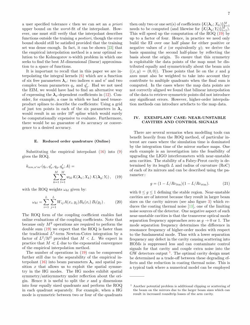
with 0 ≤ g ≤ 1 defining the stable region. Near-unstablecavities are of interest because they result in larger beamsizes on the cavity mirrors (see also figure 3) which re-duces the coating thermal noise [11], one of the limitingnoise sources of the detector. One negative aspect of suchnear-unstable cavities is that the transverse optical modeseparation frequency approaches zero as g → 0 or 1. Themode separation frequency determines the difference inresonance frequency of higher-order modes with respectto the fundamental mode. Thus with a lower separationfrequency any defect in the cavity causing scattering intoHOMs is suppressed less and can contaminate controlsignals for that cavity and couple extra noise into theGW detectors output 1. The optimal cavity design mustbe determined as a trade-off between these degrading ef-fects and the reduction in coating thermal noise. This isa typical task where a numerical model can be employed

1 Another potential problem is additional clipping or scattering ofthe beam on the mirrors due to the larger beam sizes which canresult in increased roundtrip losses of the arm cavity.

8

−15 −10 05 0 5 10 15

Separation frequency [kHz]

0.70

0.75

0.80

0.85

0.90

0.95

Cavi

ty s

tab

l t

y, g

0

10

20

30

40

50

60

70

80

90

Ch

an

ge n

RoC

[m

]

050 0 50

ETM tun ng [deg]

10-5 10-4 10-3 10-2 10-1 100 101 102

Circulating power [W]

(a) Cavity scan as ITM and ETM RoC varied

−15 −10 −5 0 5 10 15

Separation frequency [kHz]

0.70

0.75

0.80

0.85

0.90

0.95

Cavi

ty s

tab

i it

y

−50 0 50

ETM tuning [deg]

0

10

20

30

40

50

60

70

80

90

Ch

an

ge in

RoC

[m

]

10-14 10-13 10-12 10-11 10-10

Relative error

(b) The relative error between ROQ and Newton-Cotes.

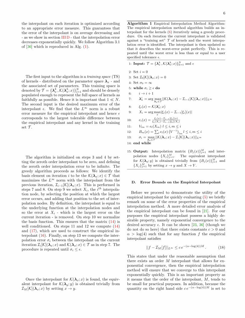
Figure 2: Modeled LIGO cavity scan as the RoC of the ITM and ETM are varied to make the cavity increasingly moreunstable. This simulation was run for Omax = 10 and includes clipping from the finite size of the mirrors and surface

imperfections from the ETM08 and ITM04 maps. Figure 2a shows how the amount of power scattering into HOM changes asg → 1. Also visible here is the reduction in the mode separation frequency with increasing instability. The contribution of theTEM00 mode has been removed to make the HOM content more visible. The reduced basis was built for mode order O = 14,

to reduce errors, see figure 7. The difference in this result when using ROQ compared to Newton-Cotes is shown in 2b.

0.70 0.75 0.80 0.85 0.90 0.95

Cavity stability

40

60

80

100

120

140

160

w(z)[m

m]

Beam size in cavity

ETMITM

Figure 3: The beam size on the ITM and ETM of a LIGOcavity as a function of cavity stability parameter as the

mirror RoCs are tuned.

to search the parameter space. In this case each pointin that parameter space corresponds to a different beamsize in the cavity which forces a re-computation of thescattering matrices on the mirrors. Thus the new algo-rithm described in this paper should yield a significantreduction in computing time.

In this section we briefly summarise the results fromthe simulations and in the following section we providethe details of setting up the model and give an analysis

of the performance of the ROQ algorithm. We have im-plemented the ROQ integration in our open-source sim-ulation tool Finesse and use the official input parame-ter files for the LIGO detectors [20]. Below we show thepreliminary investigation of the behaviour of a single Ad-vanced LIGO like arm cavity with a finesse of 450, wherethe mirror maps for the mirrors ETM08 and ITM04 2

were applied to the high reflective (HR) surfaces. Notethat we do not report the scientific results of the sim-ulation task which will be published elsewhere. Thisexample is representative for a class of modelling per-formed regularly for the LIGO commissioning and de-sign and provides us with a concrete and quantitive setupto demonstrate the required steps to use the ROQ algo-rithm.

Modelling the LIGO cavity for differing stabilities in-volves varying the RoC of both the ITM and ETM.The resulting change in w(z) at each surface means thescattering matrices will need to be recomputed for eachstate we choose. To view the HOM content in the cav-ity created by the scattering a cavity scan can be per-formed, displacing one of the cavity mirrors along the

2 The nominal radius of curvatures of ETM08 and ITM04 are1934m and 2245m respectively. The optical properties of thesemirrors were taken from [25].

9

−4 −2 0 2 4

Differential arm [deg]

−10

−5

0

5

10Er

ror

sign

al[W]

Evolution of Error signal

0.90

0.92

0.94

0.96

0.98

1.00

Cav

ity

stab

ility

,g

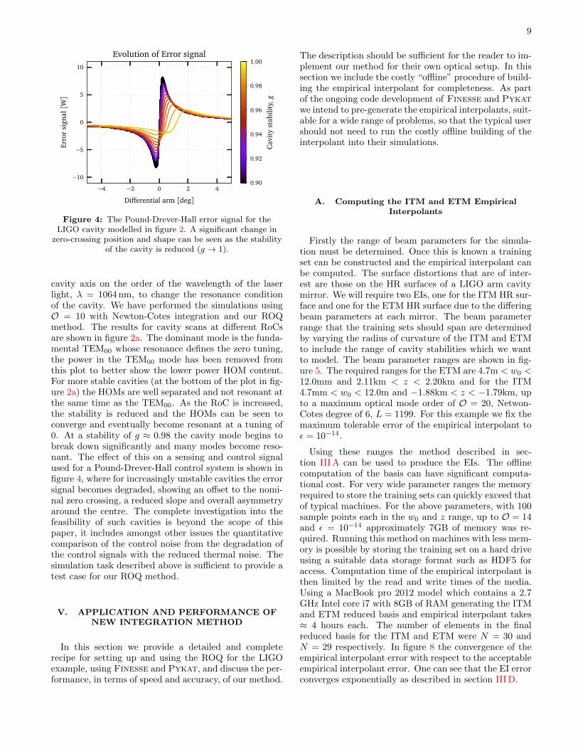
Figure 4: The Pound-Drever-Hall error signal for theLIGO cavity modelled in figure 2. A significant change in

zero-crossing position and shape can be seen as the stabilityof the cavity is reduced (g → 1).

cavity axis on the order of the wavelength of the laserlight, λ = 1064 nm, to change the resonance conditionof the cavity. We have performed the simulations usingO = 10 with Newton-Cotes integration and our ROQmethod. The results for cavity scans at different RoCsare shown in figure 2a. The dominant mode is the funda-mental TEM00 whose resonance defines the zero tuning,the power in the TEM00 mode has been removed fromthis plot to better show the lower power HOM content.For more stable cavities (at the bottom of the plot in fig-ure 2a) the HOMs are well separated and not resonant atthe same time as the TEM00. As the RoC is increased,the stability is reduced and the HOMs can be seen toconverge and eventually become resonant at a tuning of0. At a stability of g ≈ 0.98 the cavity mode begins tobreak down significantly and many modes become reso-nant. The effect of this on a sensing and control signalused for a Pound-Drever-Hall control system is shown infigure 4, where for increasingly unstable cavities the errorsignal becomes degraded, showing an offset to the nomi-nal zero crossing, a reduced slope and overall asymmetryaround the centre. The complete investigation into thefeasibility of such cavities is beyond the scope of thispaper, it includes amongst other issues the quantitativecomparison of the control noise from the degradation ofthe control signals with the reduced thermal noise. Thesimulation task described above is sufficient to provide atest case for our ROQ method.

V. APPLICATION AND PERFORMANCE OFNEW INTEGRATION METHOD

In this section we provide a detailed and completerecipe for setting up and using the ROQ for the LIGOexample, using Finesse and Pykat, and discuss the per-formance, in terms of speed and accuracy, of our method.

The description should be sufficient for the reader to im-plement our method for their own optical setup. In thissection we include the costly “offline” procedure of build-ing the empirical interpolant for completeness. As partof the ongoing code development of Finesse and Pykatwe intend to pre-generate the empirical interpolants, suit-able for a wide range of problems, so that the typical usershould not need to run the costly offline building of theinterpolant into their simulations.

A. Computing the ITM and ETM EmpiricalInterpolants

Firstly the range of beam parameters for the simula-tion must be determined. Once this is known a trainingset can be constructed and the empirical interpolant canbe computed. The surface distortions that are of inter-est are those on the HR surfaces of a LIGO arm cavitymirror. We will require two EIs, one for the ITM HR sur-face and one for the ETM HR surface due to the differingbeam parameters at each mirror. The beam parameterrange that the training sets should span are determinedby varying the radius of curvature of the ITM and ETMto include the range of cavity stabilities which we wantto model. The beam parameter ranges are shown in fig-ure 5. The required ranges for the ETM are 4.7m < w0 <12.0mm and 2.11km < z < 2.20km and for the ITM4.7mm < w0 < 12.0m and −1.88km < z < −1.79km, upto a maximum optical mode order of O = 20, Netwon-Cotes degree of 6, L = 1199. For this example we fix themaximum tolerable error of the empirical interpolant toε = 10−14.

Using these ranges the method described in sec-tion III A can be used to produce the EIs. The offlinecomputation of the basis can have significant computa-tional cost. For very wide parameter ranges the memoryrequired to store the training sets can quickly exceed thatof typical machines. For the above parameters, with 100sample points each in the w0 and z range, up to O = 14and ε = 10−14 approximately 7GB of memory was re-quired. Running this method on machines with less mem-ory is possible by storing the training set on a hard driveusing a suitable data storage format such as HDF5 foraccess. Computation time of the empirical interpolant isthen limited by the read and write times of the media.Using a MacBook pro 2012 model which contains a 2.7GHz Intel core i7 with 8GB of RAM generating the ITMand ETM reduced basis and empirical interpolant takes≈ 4 hours each. The number of elements in the finalreduced basis for the ITM and ETM were N = 30 andN = 29 respectively. In figure 8 the convergence of theempirical interpolant error with respect to the acceptableempirical interpolant error. One can see that the EI errorconverges exponentially as described in section III D.

10

0 30 60 90

Change in ETM RoC [m]

0

30

60

90C

hang

ein

ITM

RoC[m]

0.70

0.75

0.80

0.850.90

0.95

Stability

0 30 60 90

Change in ETM RoC [m]

0

30

60

90

Cha

nge

inIT

MR

oC[m] 0.7

0.80.9

1.0

1.1

ITM/ETM waist w0 [cm]

0 30 60 90

Change in ETM RoC [m]

0

30

60

90

Cha

nge

inIT

MR

oC[m]

2.13

2.15

2.16

2.18

2.19

ETM z [km]

0 30 60 90

Change in ETM RoC [m]

0

30

60

90

Cha

nge

inIT

MR

oC[m]

-1.8

6-1

.84

-1.8

3-1

.81

ITM z [km]

Figure 5: Range of beam parameters needed to model a change in curvature from 0 m to 90 m at the ITM and the ETM. Inorder to utilise the ROQ to cover this parameter space, the empirical interpolant needs to be constructed using a training set

made from kernels (6) densely covering this space.

B. Producing the ROQ weights

Once the empirical interpolant has been computed forboth ITM and ETM HR surfaces the ROQ weights (20)can be computed by convoluting the mirror maps withthe interpolant. The surface maps that we have chosenare the measured surface distortions of the (uncoated)test masses currently installed at the LIGO Livingstonobservatory, shown in figure 1. The maps contain L ≈1200 samples and we can expect a theoretical speed-upof L2/N2 ≈ 12002/302 = 1600 from using ROQ overNewton-Cotes. These maps include an aperture, A, andthe variation in surface height in meters, z(x, y). Thusto calculate the HOM scattering on reflection from oneof these mirrors with (5) the distortion term is:

A(x, y) = A(x, y)e2ikz(x,y) (22)

where A(x, y) is 1 if√x2 + y2 < 0.16m and 0 otherwise,

and k is the wavenumber of the incident optical field.Using (22) with equation (20) (with a Newton-Cotes

rule of the same degree the empirical interpolant was gen-erated with) the ROQ weights can be computed for eachmap shown in figure 1. This computational cost is pro-portional to the number of elements in the EI, M , and thenumber of samples in the map, L2. For the LIGO mapsthis takes ≈ 10s on our 2012 MacBook Pro. The result-ing ROQ rule for the maps can be visualised as shown infigure 6: the amplitude of the ROQ weights map out theaperture and the phase of the weights varies for differentmaps because of the different surface structure. The com-putation of these ROQ weights need only be performedonce for each map, unless the range of beam parametersrequired for the empirical interpolant are changed.

We verify that the process of generating the ROQ rulehas worked correctly by computing the scattering ma-trices with ROQ and Newton-Cotes across the parame-

ter space. We compute k(q; ETM07) with Omax = 10using ROQ and then again using Newton-Cotes integra-tion. Computing the relative error between each elementof these two matrices the maximum error can be takenfor q values spanning the requested q parameter range.

Figure 9 shows how the final error of the EI, σM , propa-gates into an error in the scattering matrix. This showsthe maximum (solid line) and minimum (dashed line) er-rors for any element in the scattering matrix betweenthe two methods. From this it can be seen that buildinga more accurate empirical interpolant results in smallermaximum errors in the scattering matrix. Now, usingthe most accurate reduced basis the maximum relativeerror is shown in figure 7 over the q space, where thewhite dashed box shows the boundaries of the parame-ters in the training set. Overall the method successfullycomputed a ROQ rule that accurately reproduced theNewton-Cotes results for scattering up to O = 10. Inshould be notes that the largest errors, e.g. as seen infigure 9, do not represent the full parameter space butoccur only at smallest z and largest w0. It was also foundthat building a basis including a higher maximum HOM,for example basis of order 14 for scattering computationsup to order 10, significantly improved the accuracy ofthe ROQ. Using an reduced basis constructed for order14 rather than order 10 only increased the number of el-ements in the basis by 2, thus not significantly degradingany speed improvements. It can also be seen in figure 7that ROQ extrapolates beyond the originally requestedq parameter space and does not instantly fail for evalu-ations outside of it. A gradual decrease in the accuracycan be seen when using larger w0 values.

C. Performance

The time taken to run these Finesse simulations asO is increased is shown in figure 10 demonstrating howmuch more efficient it is to use ROQ over Newton-Cotesfor the computation of scattering matrices. We also showfor reference the computation time when no scatteringfrom surface maps is included to give the base time ittakes to run the rest of the Finesse simulation. Theoverall speed-up achieved can be seen in figure 11, reach-ing ≈ 2700 times faster to run the entire simulationat O = 10. The overall speed-up then begins to dropslightly as the base time taken to run the rest of Finesse

11

−15.0 −7.5 0.0 7.5 15.0

x [cm]

−15.0

−7.5

0.0

7.5

15.0

y[c

m]

ETM07 weights|w|

−15.0 −7.5 0.0 7.5 15.0

x [cm]

−15.0

−7.5

0.0

7.5

15.0

y[c

m]

log10(|arg(w)|)

−15.0 −7.5 0.0 7.5 15.0

x [cm]

−15.0

−7.5

0.0

7.5

15.0

y[c

m]

ETM09 weights|w|

−15.0 −7.5 0.0 7.5 15.0

x [cm]

−15.0

−7.5

0.0

7.5

15.0

y[c

m]

log10(|arg(w)|)

−15.0 −7.5 0.0 7.5 15.0

x [cm]

−15.0

−7.5

0.0

7.5

15.0

y[c

m]

ITM04 weights|w|

−15.0 −7.5 0.0 7.5 15.0

x [cm]

−15.0

−7.5

0.0

7.5

15.0

y[c

m]

log10(|arg(w)|)

−15.0 −7.5 0.0 7.5 15.0

x [cm]

−15.0

−7.5

0.0

7.5

15.0

y[c

m]

ITM08 weights|w|

−15.0 −7.5 0.0 7.5 15.0

x [cm]

−15.0

−7.5

0.0

7.5

15.0

y[c

m]

log10(|arg(w)|)

10−5

10−4

10−3

10−2

10−1

100

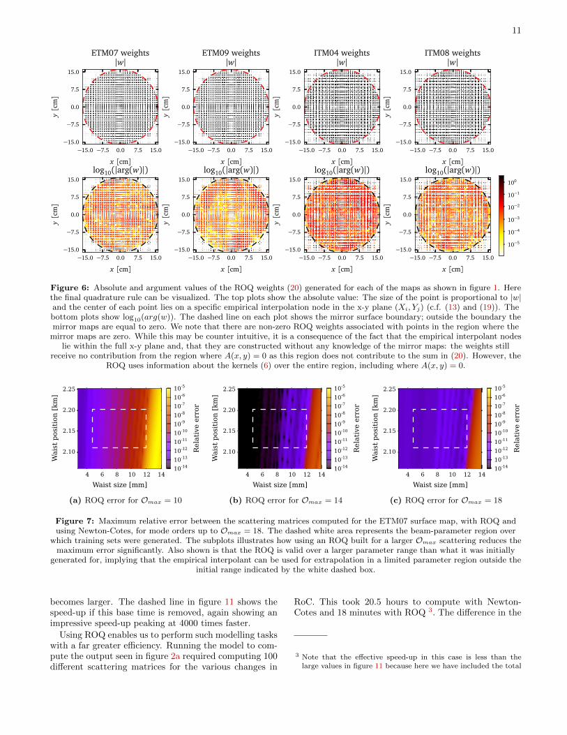
Figure 6: Absolute and argument values of the ROQ weights (20) generated for each of the maps as shown in figure 1. Herethe final quadrature rule can be visualized. The top plots show the absolute value: The size of the point is proportional to |w|and the center of each point lies on a specific empirical interpolation node in the x-y plane (Xi, Yj) (c.f. (13) and (19)). Thebottom plots show log10(arg(w)). The dashed line on each plot shows the mirror surface boundary; outside the boundary themirror maps are equal to zero. We note that there are non-zero ROQ weights associated with points in the region where the

mirror maps are zero. While this may be counter intuitive, it is a consequence of the fact that the empirical interpolant nodeslie within the full x-y plane and, that they are constructed without any knowledge of the mirror maps: the weights still

receive no contribution from the region where A(x, y) = 0 as this region does not contribute to the sum in (20). However, theROQ uses information about the kernels (6) over the entire region, including where A(x, y) = 0.

4 6 8 10 12 14

Waist size [mm]

2.10

2.15

2.20

2.25

Waist position [km]

10-1410-1310-1210-1110-1010-910-810-710-610-5

Relative

error

(a) ROQ error for Omax = 10

4 6 8 10 12 14

Waist size [mm]

2.10

2.15

2.20

2.25

Waist position [km]

10-1410-1310-1210-1110-1010-910-810-710-610-5

Relative

error

(b) ROQ error for Omax = 14

4 6 8 10 12 14

Waist size [mm]

2.10

2.15

2.20

2.25

Waist position [km]

10-1410-1310-1210-1110-1010-910-810-710-610-5

Relative

error

(c) ROQ error for Omax = 18

Figure 7: Maximum relative error between the scattering matrices computed for the ETM07 surface map, with ROQ andusing Newton-Cotes, for mode orders up to Omax = 18. The dashed white area represents the beam-parameter region over

which training sets were generated. The subplots illustrates how using an ROQ built for a larger Omax scattering reduces themaximum error significantly. Also shown is that the ROQ is valid over a larger parameter range than what it was initially

generated for, implying that the empirical interpolant can be used for extrapolation in a limited parameter region outside theinitial range indicated by the white dashed box.

becomes larger. The dashed line in figure 11 shows thespeed-up if this base time is removed, again showing animpressive speed-up peaking at 4000 times faster.

Using ROQ enables us to perform such modelling taskswith a far greater efficiency. Running the model to com-pute the output seen in figure 2a required computing 100different scattering matrices for the various changes in

RoC. This took 20.5 hours to compute with Newton-Cotes and 18 minutes with ROQ 3. The difference in the

3 Note that the effective speed-up in this case is less than thelarge values in figure 11 because here we have included the total

12

18 20 22 24 26 28 30

Basis size

10−14

10−13

10−12

10−11

10−10

10−9

10−8

10−7

10−6EI

erro

r,σ

METMITM

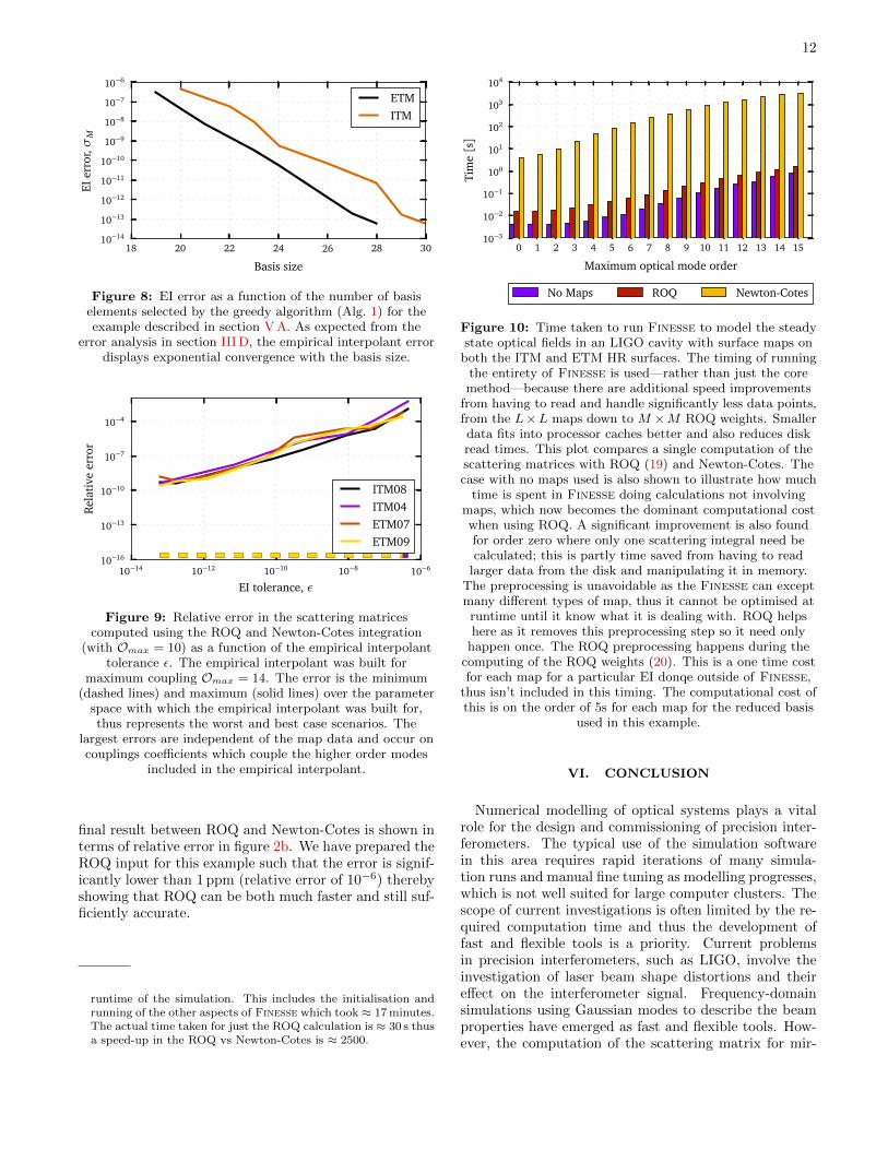
Figure 8: EI error as a function of the number of basiselements selected by the greedy algorithm (Alg. 1) for theexample described in section V A. As expected from the

error analysis in section III D, the empirical interpolant errordisplays exponential convergence with the basis size.

10−14 10−12 10−10 10−8 10−6

EI tolerance, ε

10−16

10−13

10−10

10−7

10−4

Rel

ativ

eer

ror

ITM08ITM04ETM07ETM09

Figure 9: Relative error in the scattering matricescomputed using the ROQ and Newton-Cotes integration

(with Omax = 10) as a function of the empirical interpolanttolerance ε. The empirical interpolant was built for

maximum coupling Omax = 14. The error is the minimum(dashed lines) and maximum (solid lines) over the parameter

space with which the empirical interpolant was built for,thus represents the worst and best case scenarios. The

largest errors are independent of the map data and occur oncouplings coefficients which couple the higher order modes

included in the empirical interpolant.

final result between ROQ and Newton-Cotes is shown interms of relative error in figure 2b. We have prepared theROQ input for this example such that the error is signif-icantly lower than 1 ppm (relative error of 10−6) therebyshowing that ROQ can be both much faster and still suf-ficiently accurate.

runtime of the simulation. This includes the initialisation andrunning of the other aspects of Finesse which took ≈ 17 minutes.The actual time taken for just the ROQ calculation is ≈ 30 s thusa speed-up in the ROQ vs Newton-Cotes is ≈ 2500.

0 1 2 3 4 5 6 7 8 9 10 11 12 13 14 15

Maximum optical mode order

10−3

10−2

10−1

100

101

102

103

104

Tim

e[s]

No Maps ROQ Newton-Cotes

Figure 10: Time taken to run Finesse to model the steadystate optical fields in an LIGO cavity with surface maps on

both the ITM and ETM HR surfaces. The timing of runningthe entirety of Finesse is used—rather than just the coremethod—because there are additional speed improvements

from having to read and handle significantly less data points,from the L×L maps down to M ×M ROQ weights. Smallerdata fits into processor caches better and also reduces diskread times. This plot compares a single computation of thescattering matrices with ROQ (19) and Newton-Cotes. Thecase with no maps used is also shown to illustrate how much

time is spent in Finesse doing calculations not involvingmaps, which now becomes the dominant computational costwhen using ROQ. A significant improvement is also foundfor order zero where only one scattering integral need becalculated; this is partly time saved from having to read

larger data from the disk and manipulating it in memory.The preprocessing is unavoidable as the Finesse can exceptmany different types of map, thus it cannot be optimised atruntime until it know what it is dealing with. ROQ helpshere as it removes this preprocessing step so it need only

happen once. The ROQ preprocessing happens during thecomputing of the ROQ weights (20). This is a one time costfor each map for a particular EI donqe outside of Finesse,

thus isn’t included in this timing. The computational cost ofthis is on the order of 5s for each map for the reduced basis

used in this example.

VI. CONCLUSION

Numerical modelling of optical systems plays a vitalrole for the design and commissioning of precision inter-ferometers. The typical use of the simulation softwarein this area requires rapid iterations of many simula-tion runs and manual fine tuning as modelling progresses,which is not well suited for large computer clusters. Thescope of current investigations is often limited by the re-quired computation time and thus the development offast and flexible tools is a priority. Current problemsin precision interferometers, such as LIGO, involve theinvestigation of laser beam shape distortions and theireffect on the interferometer signal. Frequency-domainsimulations using Gaussian modes to describe the beamproperties have emerged as fast and flexible tools. How-ever, the computation of the scattering matrix for mir-

13

0 2 4 6 8 10 12 14 16

Maximum optical mode order

0

500

1000

1500

2000

2500

3000

3500

4000

4500R

OQ

Spee

dup

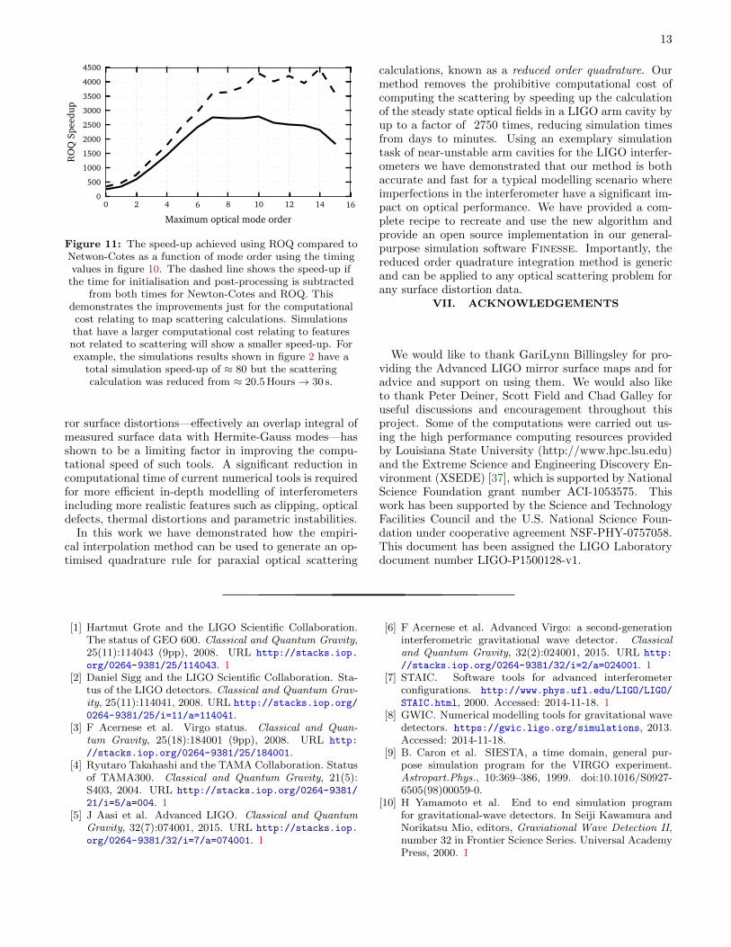
Figure 11: The speed-up achieved using ROQ compared toNetwon-Cotes as a function of mode order using the timingvalues in figure 10. The dashed line shows the speed-up if

the time for initialisation and post-processing is subtractedfrom both times for Newton-Cotes and ROQ. This

demonstrates the improvements just for the computationalcost relating to map scattering calculations. Simulationsthat have a larger computational cost relating to featuresnot related to scattering will show a smaller speed-up. Forexample, the simulations results shown in figure 2 have a

total simulation speed-up of ≈ 80 but the scatteringcalculation was reduced from ≈ 20.5 Hours→ 30 s.

ror surface distortions—effectively an overlap integral ofmeasured surface data with Hermite-Gauss modes—hasshown to be a limiting factor in improving the compu-tational speed of such tools. A significant reduction incomputational time of current numerical tools is requiredfor more efficient in-depth modelling of interferometersincluding more realistic features such as clipping, opticaldefects, thermal distortions and parametric instabilities.

In this work we have demonstrated how the empiri-cal interpolation method can be used to generate an op-timised quadrature rule for paraxial optical scattering

calculations, known as a reduced order quadrature. Ourmethod removes the prohibitive computational cost ofcomputing the scattering by speeding up the calculationof the steady state optical fields in a LIGO arm cavity byup to a factor of 2750 times, reducing simulation timesfrom days to minutes. Using an exemplary simulationtask of near-unstable arm cavities for the LIGO interfer-ometers we have demonstrated that our method is bothaccurate and fast for a typical modelling scenario whereimperfections in the interferometer have a significant im-pact on optical performance. We have provided a com-plete recipe to recreate and use the new algorithm andprovide an open source implementation in our general-purpose simulation software Finesse. Importantly, thereduced order quadrature integration method is genericand can be applied to any optical scattering problem forany surface distortion data.

VII. ACKNOWLEDGEMENTS

We would like to thank GariLynn Billingsley for pro-viding the Advanced LIGO mirror surface maps and foradvice and support on using them. We would also liketo thank Peter Deiner, Scott Field and Chad Galley foruseful discussions and encouragement throughout thisproject. Some of the computations were carried out us-ing the high performance computing resources providedby Louisiana State University (http://www.hpc.lsu.edu)and the Extreme Science and Engineering Discovery En-vironment (XSEDE) [37], which is supported by NationalScience Foundation grant number ACI-1053575. Thiswork has been supported by the Science and TechnologyFacilities Council and the U.S. National Science Foun-dation under cooperative agreement NSF-PHY-0757058.This document has been assigned the LIGO Laboratorydocument number LIGO-P1500128-v1.

[1] Hartmut Grote and the LIGO Scientific Collaboration.The status of GEO 600. Classical and Quantum Gravity,25(11):114043 (9pp), 2008. URL http://stacks.iop.

org/0264-9381/25/114043. 1[2] Daniel Sigg and the LIGO Scientific Collaboration. Sta-

tus of the LIGO detectors. Classical and Quantum Grav-ity, 25(11):114041, 2008. URL http://stacks.iop.org/

0264-9381/25/i=11/a=114041.[3] F Acernese et al. Virgo status. Classical and Quan-

tum Gravity, 25(18):184001 (9pp), 2008. URL http:

//stacks.iop.org/0264-9381/25/184001.[4] Ryutaro Takahashi and the TAMA Collaboration. Status

of TAMA300. Classical and Quantum Gravity, 21(5):S403, 2004. URL http://stacks.iop.org/0264-9381/

21/i=5/a=004. 1[5] J Aasi et al. Advanced LIGO. Classical and Quantum

Gravity, 32(7):074001, 2015. URL http://stacks.iop.

org/0264-9381/32/i=7/a=074001. 1

[6] F Acernese et al. Advanced Virgo: a second-generationinterferometric gravitational wave detector. Classicaland Quantum Gravity, 32(2):024001, 2015. URL http:

//stacks.iop.org/0264-9381/32/i=2/a=024001. 1[7] STAIC. Software tools for advanced interferometer

configurations. http://www.phys.ufl.edu/LIGO/LIGO/

STAIC.html, 2000. Accessed: 2014-11-18. 1[8] GWIC. Numerical modelling tools for gravitational wave

detectors. https://gwic.ligo.org/simulations, 2013.Accessed: 2014-11-18.

[9] B. Caron et al. SIESTA, a time domain, general pur-pose simulation program for the VIRGO experiment.Astropart.Phys., 10:369–386, 1999. doi:10.1016/S0927-6505(98)00059-0.

[10] H Yamamoto et al. End to end simulation programfor gravitational-wave detectors. In Seiji Kawamura andNorikatsu Mio, editors, Graviational Wave Detection II,number 32 in Frontier Science Series. Universal AcademyPress, 2000. 1

14

[11] Jean-Yves Vinet. On special optical modes and thermalissues in advanced gravitational wave interferometric de-tectors. Living Reviews in Relativity, 12(5), 2009. URLhttp://www.livingreviews.org/lrr-2009-5. 1, 7

[12] J.-Y. Vinet, P. Hello, C. N. Man, and A. Brillet. A highaccuracy method for the simulation of non-ideal opticalcavities. Journal de Physique I, 2:1287–1303, July 1992.doi:10.1051/jp1:1992211. 1

[13] Raymond G. Beausoleil et al. Model of thermalwave-front distortion in interferometric gravitational-wave detectors. i. thermal focusing. J. Opt.Soc. Am. B, 20(6):1247–1268, Jun 2003. doi:10.1364/JOSAB.20.001247. URL http://josab.osa.

org/abstract.cfm?URI=josab-20-6-1247. 1[14] ET science team. Einstein gravitational wave telescope

conceptual design study. Technical Report ET-0106C-10,2010, https://tds.ego-gw.it/itf/tds/. 1

[15] Schibli T R et al. Optical frequency comb with sub-millihertz linewidth and more than 10 w average power.Nature Photonics, 2:355 – 359, 2008. 1

[16] Susannah M. Dickerson, Jason M. Hogan, Alex Sugar-baker, David M. S. Johnson, and Mark A. Kasevich. Mul-tiaxis inertial sensing with long-time point source atominterferometry. Phys. Rev. Lett., 111:083001, Aug 2013.doi:10.1103/PhysRevLett.111.083001. 1

[17] A. Freise and K. Strain. Interferometer Techniques forGravitational-Wave Detection. Living Reviews in Rela-tivity, 13:1–+, February 2010. URL http://relativity.

livingreviews.org/Articles/lrr-010-1/2. 1[18] Charlotte Bond, Paul Fulda, Daniel Brown, and Andreas

Freise. Investigation of beam clipping in the power recy-cling cavity of Advanced LIGO using Finesse. TechnicalReport LIGO Document T1300954, Nov 2013. 2, 3

[19] A Freise et al. Frequency-domain interferometer sim-ulation with higher-order spatial modes. Classical andQuantum Gravity, 21(5):S1067–S1074, 2004. URL http:

//stacks.iop.org/0264-9381/21/S1067. The programis available at http://www.gwoptics.org/finesse. 2

[20] Finesse input files for Advanced LIGO. https://dcc.

ligo.org/LIGO-L1300231. Accessed: 2015-07-13. 2, 8[21] Harbir Antil, ScottE. Field, Frank Herrmann, RicardoH.

Nochetto, and Manuel Tiglio. Two-step greedy algo-rithm for reduced order quadratures. Journal of ScientificComputing, 57(3):604–637, 2013. ISSN 0885-7474. doi:10.1007/s10915-013-9722-z. URL http://dx.doi.org/

10.1007/s10915-013-9722-z. 2, 4, 6[22] Priscilla Canizares et al. Accelerated gravitational

wave parameter estimation with reduced order mod-eling. Phys. Rev. Lett., 114:071104, Feb 2015. doi:10.1103/PhysRevLett.114.071104. URL http://link.

aps.org/doi/10.1103/PhysRevLett.114.071104. 2, 4[23] Y. Maday, N. C. Nguyen, A. T. Patera, and S. H. Pau. A

general multipurpose interpolation procedure: the magicpoints. Communications on Pure and Applied Analysis,8:383–404, 2009. doi:10.3934/cpaa.2009.8.383. 2, 6, 7

[24] Herwig Kogelnik. On the propagation of Gaussianbeams of light through lenslike media including thosewith a loss or gain variation. Appl. Opt., 4(12):1562–1569, 1965. URL http://ao.osa.org/abstract.cfm?

URI=ao-4-12-1562. 2, 3

[25] G. Billingsley. LIGO core optics reference page. https:

//galaxy.ligo.caltech.edu/optics/. Accessed: 2015-07-13. 3, 4, 8

[26] Charlotte Zoe Bond. How to stay in shape: overcomingbeam and mirror distortions in advanced gravitationalwave interferometers. July 2014. URL http://etheses.

bham.ac.uk/5223/. 3[27] F. Bayer-Helms. Coupling coefficients of an incident wave

and the modes of spherical optical resonator in the caseof mismatching and misalignment. Appl. Opt., 23:1369–1380, May 1984. 3

[28] J. Y. Vinet and the Virgo Collaboration. The Virgo Bookof Physics: Optics and Related Topics. Virgo, 2001. URLhttp://wwwcascina.virgo.infn.it/vpb/. 3

[29] A. Ralston and P. Rabinowitz. A First Course in Nu-merical Analysis. Dover books on mathematics. DoverPublications, 2001. ISBN 9780486414546. URL https:

//books.google.co.uk/books?id=czHV-1bEFl0C. 4[30] Maxime Barrault, Yvon Maday, Ngoc Cuong Nguyen,

and Anthony T. Patera. An empirical interpolationmethod: application to efficient reduced-basis discretiza-tion of partial differential equations. Comptes RendusMathematique, 339(9):667 – 672, 2004. ISSN 1631-073X.doi:http://dx.doi.org/10.1016/j.crma.2004.08.006. URLhttp://www.sciencedirect.com/science/article/

pii/S1631073X04004248. 4, 5[31] Jan S. Hesthaven, Benjamin Stamm, and Shun Zhang.

Efficient greedy algorithms for high-dimensional param-eter spaces with applications to empirical interpolationand reduced basis methods. ESAIM: MathematicalModelling and Numerical Analysis, 48:259–283, 12014. ISSN 1290-3841. doi:10.1051/m2an/2013100.URL http://www.esaim-m2an.org/action/article_

S0764583X13001003. 5[32] Max D. Gunzburger, Janet S. Peterson, and John N.

Shadid. Reduced-order modeling of time-dependent{PDEs} with multiple parameters in the boundarydata. Computer Methods in Applied Mechanics andEngineering, 196(46):1030 – 1047, 2007. ISSN 0045-7825.doi:http://dx.doi.org/10.1016/j.cma.2006.08.004. URLhttp://www.sciencedirect.com/science/article/

pii/S0045782506002337. 5[33] B. S. Kirk, J. W. Peterson, R. H. Stogner, and G. F.

Carey. libMesh: A C++ Library for Parallel AdaptiveMesh Refinement/Coarsening Simulations. Engineeringwith Computers, 22(3–4):237–254, 2006. 5

[34] William H. Press, Saul A. Teukolsky, William T. Vet-terling, and Brian P. Flannery. Numerical Recipes 3rdEdition: The Art of Scientific Computing. CambridgeUniversity Press, New York, NY, USA, 3 edition, 2007.ISBN 0521880688, 9780521880688. 5

[35] Kendall Atkinson. An Introduction to Numerical Analy-sis. Wiley, 2 edition. ISBN 0471624896. 5

[36] Tor Øvstedal Aanonsen. Empirical interpolation withapplication to reduced basis approximations. 2009. 6

[37] John Towns et al. Xsede: Accelerating scientificdiscovery. Computing in Science and Engineer-ing, 16(5):62–74, 2014. ISSN 1521-9615. doi:http://doi.ieeecomputersociety.org/10.1109/MCSE.2014.80.13