Embed Size (px)
Citation preview
FAST SIMULATION OF LARGE-SCALE GROWTH MODELS
TOBIAS FRIEDRICH AND LIONEL LEVINE
Abstract. We give an algorithm that computes the final state of certain growthmodels without computing all intermediate states. Our technique is based on a“least action principle” which characterizes the odometer function of the growthprocess. Starting from an educated guess for the odometer, we successively correctunder- and overestimates and provably arrive at the correct final state. The degreeof speedup depends on the accuracy of the initial guess.
Determining the size of the boundary fluctuations in internal diffusion-limitedaggregation is a long-standing open problem in statistical physics. As an applicationof our method, we calculate the size of fluctuations over two orders of magnitudebeyond previous simulations. Our data strongly support the conjecture that thefluctuations are logarithmic in the radius.
1. Introduction
In this paper we study the abelian stack model, a type of growth process on graphs.Special cases include internal diffusion limited aggregation (IDLA) and rotor-routeraggregation. We describe a method for computing the final state of the process, givenan initial guess. The more accurate the guess, the faster the computation.
IDLA. Starting with N particles at the origin of the two-dimensional square grid Z2,each particle in turn performs a simple random walk until reaching an unoccupied site.Introduced by Meakin and Deutch [26] and independently by Diaconis and Fulton[9], IDLA models physical phenomena such as solid melting around a heat source,electrochemical polishing, and fluid flow in a Hele-Shaw cell. Lawler, Bramson, andGriffeath [21] showed that as N → ∞, the asymptotic shape of the resulting clusterof N occupied sites is a disk (and in higher dimensions, a Euclidean ball).
The boundary of an IDLA cluster is a natural model of a rough propagating front(Figure 1, left). From this perspective, the most basic question one could ask is,what is the scale of the fluctuations around the limiting circular shape? The answeris believed to be logarithmic in the radius r, but the current best rigorous boundsscale as r1/3 times a logarithmic factor [20]. Determining the size of these boundaryfluctuations is a long-standing open problem in statistical physics.
Rotor-router aggregation. James Propp [18] proposed the following way of deran-domizing IDLA. At each lattice site in Z2 is a rotor that can point North, East, Southor West. Instead of stepping in a random direction, a particle rotates the rotor at itscurrent location counterclockwise, and then steps in the direction of this rotor. Each
Date: June 4, 2010.2010 Mathematics Subject Classification. 82C24, 05C81, 05C85.Key words and phrases. Cycle popping, internal diffusion limited aggregation, least action principle,
low discrepancy random stack, odometer function, potential kernel, rotor-router model.The second author was partly supported by a National Science Foundation Postdoctoral Fellowship.
1
2 TOBIAS FRIEDRICH AND LIONEL LEVINE
Figure 1. IDLA cluster (left) and rotor-router aggregation with counterclockwise rotor sequence(right) of N = 106 chips. Half of each aggregate is shown. Each site is colored according to thefinal direction of the rotor on top of its stack (yellow=W, red=S, blue=E, green=N). Note that theboundary fluctuations of the rotor-router aggregation are much smoother than for IDLA. Largerrotor-router aggregates of size up to N = 1010 can be found on [1].
of N particles starting at the origin walks in this manner until reaching an unoccupiedsite. Given the initial configuration of the rotors (which can be taken, for example,all North), the resulting growth process is entirely deterministic. Regardless of theinitial rotors, the asymptotic shape is a disk (and in higher dimensions, a Euclideanball) and the inner fluctuations are proved to be O(logN) [23]. The true fluctuationsappear to grow even more slowly, and may even be bounded independent of N .
Rotor-router aggregation is remarkable in that it generates a nearly perfect disk inthe square lattice without any reference to the Euclidean norm (x2 + y2)1/2. Perhapseven more remarkable are the patterns formed by the final directions of the rotors(Figure 1, right).
Low-discrepancy random stack. To better understand whether it is the regular-ity or the determinism which makes rotor-router aggregation so round, we follow asuggestion of James Propp and simulate a third model, low-discrepancy random stack,which combines the randomness of IDLA and the regularity of the rotor-router model.
Computing the odometer function. The central tool in our analysis of all threemodels is the odometer function, which measures the number of chips emitted fromeach site. The odometer function determines the shape of the final occupied cluster viaa nonlinear operator that we call the stack Laplacian. Our main technical contributionis that even for highly non-deterministic models such as IDLA, one can achieve fastexact calculation via intermediate approximation. Approximating our three growthprocesses by an idealized model called the divisible sandpile, we can use the knownasymptotic expansion of the potential kernel of random walk on Z2 to obtain aneducated guess of the odometer function. We present a method for carrying outsubsequent local corrections to provably transform this guess into the exact odometerfunction, and hence compute the shape of the occupied cluster.
LARGE-SCALE GROWTH MODELS 3
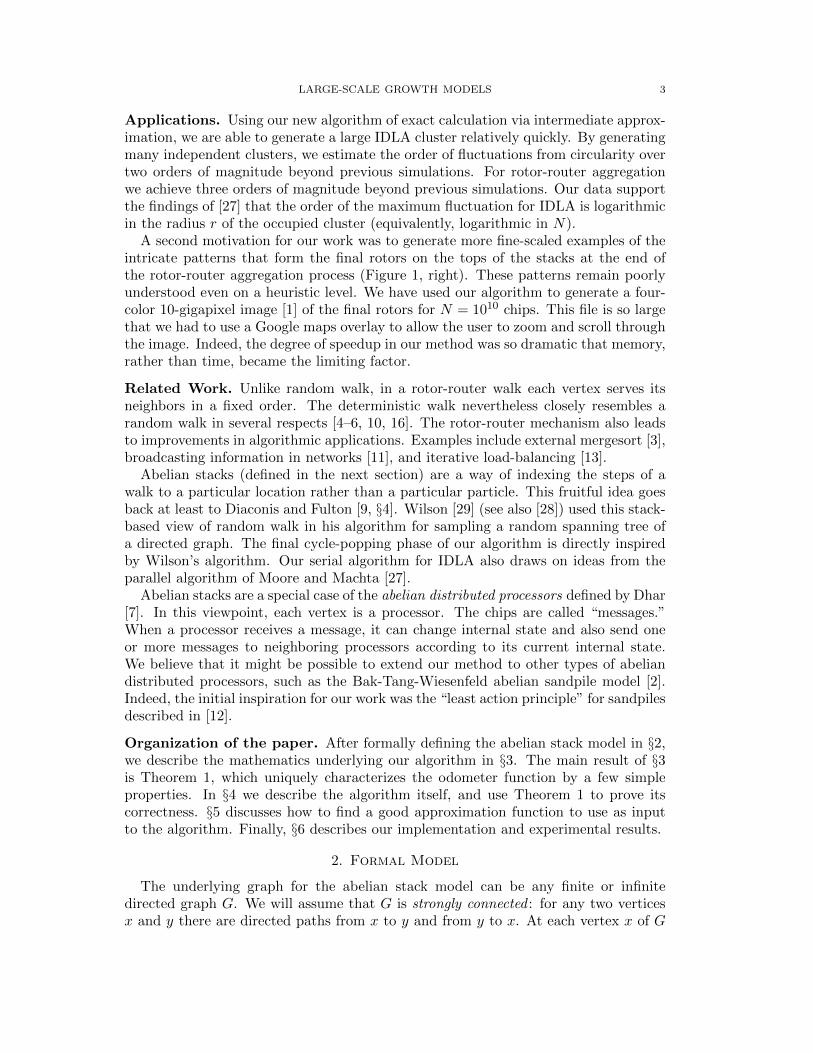
Applications. Using our new algorithm of exact calculation via intermediate approx-imation, we are able to generate a large IDLA cluster relatively quickly. By generatingmany independent clusters, we estimate the order of fluctuations from circularity overtwo orders of magnitude beyond previous simulations. For rotor-router aggregationwe achieve three orders of magnitude beyond previous simulations. Our data supportthe findings of [27] that the order of the maximum fluctuation for IDLA is logarithmicin the radius r of the occupied cluster (equivalently, logarithmic in N).
A second motivation for our work was to generate more fine-scaled examples of theintricate patterns that form the final rotors on the tops of the stacks at the end ofthe rotor-router aggregation process (Figure 1, right). These patterns remain poorlyunderstood even on a heuristic level. We have used our algorithm to generate a four-color 10-gigapixel image [1] of the final rotors for N = 1010 chips. This file is so largethat we had to use a Google maps overlay to allow the user to zoom and scroll throughthe image. Indeed, the degree of speedup in our method was so dramatic that memory,rather than time, became the limiting factor.
Related Work. Unlike random walk, in a rotor-router walk each vertex serves itsneighbors in a fixed order. The deterministic walk nevertheless closely resembles arandom walk in several respects [4–6, 10, 16]. The rotor-router mechanism also leadsto improvements in algorithmic applications. Examples include external mergesort [3],broadcasting information in networks [11], and iterative load-balancing [13].
Abelian stacks (defined in the next section) are a way of indexing the steps of awalk to a particular location rather than a particular particle. This fruitful idea goesback at least to Diaconis and Fulton [9, §4]. Wilson [29] (see also [28]) used this stack-based view of random walk in his algorithm for sampling a random spanning tree ofa directed graph. The final cycle-popping phase of our algorithm is directly inspiredby Wilson’s algorithm. Our serial algorithm for IDLA also draws on ideas from theparallel algorithm of Moore and Machta [27].
Abelian stacks are a special case of the abelian distributed processors defined by Dhar[7]. In this viewpoint, each vertex is a processor. The chips are called “messages.”When a processor receives a message, it can change internal state and also send oneor more messages to neighboring processors according to its current internal state.We believe that it might be possible to extend our method to other types of abeliandistributed processors, such as the Bak-Tang-Wiesenfeld abelian sandpile model [2].Indeed, the initial inspiration for our work was the “least action principle” for sandpilesdescribed in [12].
Organization of the paper. After formally defining the abelian stack model in §2,we describe the mathematics underlying our algorithm in §3. The main result of §3is Theorem 1, which uniquely characterizes the odometer function by a few simpleproperties. In §4 we describe the algorithm itself, and use Theorem 1 to prove itscorrectness. §5 discusses how to find a good approximation function to use as inputto the algorithm. Finally, §6 describes our implementation and experimental results.
2. Formal Model
The underlying graph for the abelian stack model can be any finite or infinitedirected graph G. We will assume that G is strongly connected : for any two verticesx and y there are directed paths from x to y and from y to x. At each vertex x of G
4 TOBIAS FRIEDRICH AND LIONEL LEVINE
is an infinite stack of rotors (ρn(x))n>0. Each rotor ρn(x) is an edge of G emanatingfrom x. We say that rotor ρ0(x) is “on top” of the stack.
A finite number of indistinguishable chips are dispersed on the vertices of G ac-cording to some prescribed initial configuration. For each vertex x, the first chip tovisit x is absorbed there and never moves again. Each subsequent chip arriving at xfirst shifts the stack at x downward, so that the new stack is ρ′n(x) = ρn+1(x). Aftershifting the stack, the chip moves to the vertex y pointed to by the rotor ρ′0(x) nowon top. We call this two-step procedure (shifting the stack and moving a chip) firingthe site x. The effect of this rule is that the n-th time a chip is emitted from x, ittravels along the edge ρn(x).
We will generally assume that the stacks are infinitive: for each edge e = (x, y),infinitely many rotors ρn(x) are equal to e. If G is infinite, or if the total numberof chips is at most the number of vertices, then this condition ensures that firingeventually stops, and all chips are absorbed.
We are interested in the set of occupied sites, that is, sites that absorb a chip. Theabelian property [9, Theorem 4.1] asserts that this set does not depend on the orderin which vertices are fired. This property plays a key role in our method; we discussit further in §3.
If the rotors ρn(x) are independent and identically distributed random edges em-anating from x, then we obtain IDLA. The special case of IDLA in which all chipsstart at a fixed vertex o is more commonly described as follows. Let A1 = o, andfor N > 2 define a random set AN of N vertices of G according to the recursive rule
AN+1 = AN ∪ xN (1)
where xN is the endpoint of a random walk started at o and stopped when it firstvisits a site not in AN . These random walks describe one particular sequence in whichthe vertices can be fired, for the initial configuration of N chips at o. The first chip isabsorbed at o, and subsequent chips are absorbed in turn at sites x1, . . . , xN−1. Whenfiring stops, the set of occupied sites is AN .
A second interesting case is deterministic: the sequence ρn(x) is periodic in n,for every vertex x. For example, on Z2, we could take the top rotor in each stackto point to the northward neighbor, the next to the eastward neighbor, and so on.This choice yields the model of rotor-router aggregation defined by Propp [18] andanalyzed in [22, 23]. It is described by the growth rule (1), where xN is the endpointof a rotor-router walk started at the origin and stopped on first exiting AN .
3. Least Action Principle
Let G = (V,E) be a locally finite directed graph, which may have loops and multipleedges. Each edge e ∈ E is oriented from its source vertex s(e) to its target vertext(e). We assume that G is strongly connected.
A rotor configuration on G is a function
r : V → E
such that s(r(v)) = v for all v ∈ V . A chip configuration on G is a function
σ : V → Z
LARGE-SCALE GROWTH MODELS 5
with finite support. Note we do not require σ > 0. If σ(x) = m > 0, we say there arem chips at vertex x; if σ(x) = −m < 0, we say there is a hole of depth m at vertex x.
For an edge e and a nonnegative integer n, let
Rρ(e, n) = #1 6 k 6 n | ρk(s(e)) = e (2)
be the number of times e occurs among the first n rotors in the stack at the vertex s(e)(excluding the top rotor ρ0(s(e))). When no ambiguity would result, we drop thesubscript ρ.
Write N for the set of nonnegative integers. Given a function u : V → N, we wouldlike to describe the net effect on chips resulting from firing each vertex x ∈ V a totalof u(x) times. In the course of these firings, each vertex x emits u(x) chips, and receivesRρ(e, u(s(e))) chips along each incoming edge e with t(e) = x. This motivates thefollowing definition.
Definition. The stack Laplacian of a function u : V → N is the function
∆ρu : V → Zgiven by
∆ρu(x) =∑
t(e)=x
Rρ(e, u(s(e)))− u(x). (3)
The sum is over all edges e with target vertex t(e) = x. We use the notation ∆ρ toemphasize the dependence (via Rρ) on the rotor stacks ρk(x).
Given an initial chip configuration σ0, the configuration σ resulting from performingu(x) firings at each site x ∈ V is given by
σ = σ0 + ∆ρu. (4)
The rotor configuration on the tops of the stacks after these firings is also easy todescribe. We denote this configuration by Topρ(u), and it is given by
Topρ(u)(x) = ρu(x)(x).
We also write Euρ for the collection of shifted stacks:
(Euρ)k(x) = ρk+u(x)(x).
The stack Laplacian is not a linear operator, but it satisfies the relation
∆ρ(u+ v) = ∆ρu+ ∆Euρv. (5)
Vertices x1, . . . , xm form a legal firing sequence for σ0 if
σj(xj+1) > 1, j = 0, . . . ,m− 1
whereσj = σ0 + ∆ρuj
anduj(x) = #i 6 j : xi = x.
In words, the condition σj(xj+1) > 1 says that after firing x1, . . . , xj , the vertex xj+1
has at least two chips. We require at least two because in our growth model, the firstchip to visit each vertex gets absorbed.
The firing sequence is complete if no further legal firings are possible; that is,σm(x) 6 1 for all x ∈ V . If x1, . . . , xm is a complete legal firing sequence for the chip
6 TOBIAS FRIEDRICH AND LIONEL LEVINE
configuration σ0, then we call the function u := um the odometer of σ0.
Abelian Property [9, Theorem 4.1] Given an initial configuration σ0 andstacks ρ, every complete legal firing sequence for σ0 has the same odometer function u.
It follows that the final chip configuration σm = σ0 + ∆ρu and the final rotorconfiguration Top(u) do not depend on the choice of complete legal firing sequence.
Given a chip configuration σ0 and rotor stacks ρk(x), our goal is to compute thefinal chip configuration σm without performing individual firings one at a time. Byequation (4), it suffices to compute the odometer function u of σ0. (In practice, it isusually easy to compute ∆ρu given u, an issue we address in §4.)
Our approach will be to start from an approximation of u and correct errors. Inorder to know when our algorithm is finished, the key mathematical point is to finda list of properties of u that characterize it uniquely. Our main result in this section,Theorem 1, gives such a list. As we now explain, the hypotheses of this theorem canall be guessed from certain necessary features of the final chip configuration σm andthe final rotor configuration Topρ(u). What is perhaps surprising is that these fewproperties suffice to characterize u.
Let x1, . . . , xm be a complete legal firing sequence for the chip configuration σ0. Westart with the observation that since no further legal firings are possible,
• σm(x) 6 1 for all x ∈ V .
Next, letA = x ∈ V : u(x) > 0
be the set of sites that fire. Since each site that fires must first absorb a chip, we have
• σm(x) = 1 for all x ∈ A.
Finally, observe that for any vertex x ∈ A, the rotor rx = Topρ(u)(x) at the top of thestack at x is the edge traversed by the last chip fired from x. In particular, for anyfinite subset A′ of A, the top rotor at the vertex of A′ that fired last points to a vertexnot in A′.
• For any finite set A′ ⊂ A, there exists x ∈ A′ with t(rx) /∈ A′.We can state this last condition more succinctly by saying that the rotor configurationr = Top(u) is acyclic on A; that is, the spanning subgraph (V, r(A)) has no directedcycles.
Theorem 1. Let G be a finite or infinite directed graph, ρ a collection of rotor stackson G, and σ0 a chip configuration on G. Let u be the corresponding odometer function.Fix u∗ : V → N, and let A∗ = x ∈ V : u∗(x) > 0. Let σ∗ = σ0 + ∆ρu∗, and supposethat
• σ∗ 6 1;• A∗ is finite;• σ∗(x) = 1 for all x ∈ A∗; and• Topρ(u∗) is acyclic on A∗.
Then u∗ = u.
Remark. To ensure that u is finite (i.e., that there exists a finite complete legal firingsequence) it is common to place some minimal assumptions on ρ and σ0. For example,if G is infinite and strongly connected, then it suffices to assume that the stacks ρ are
LARGE-SCALE GROWTH MODELS 7
infinitive. Theorem 1 does not explicitly make any assumptions of this kind; rather, ifa function u∗ exists satisfying the conditions listed, then u must be finite (and equalto u∗).
We break the proof into two inequalities. The first inequality can be seen as ananalogue for the abelian stack model of the least action principle for sandpiles [12,Lemma 2.3].
Lemma 2. (Least Action Principle) If σ∗ 6 1, then u∗ > u.
Proof. Perform legal firings in any order, without allowing any site x to fire more thanu∗(x) times, until no such firing is possible. Write u′(x) for the number of times xfires during this procedure. We will show that u′ = u.
Write σ′ = σ0 + ∆ρu′. If σ′ 6 1, then u′ = u by the abelian property. Otherwise,
choose y such that σ′(y) > 1. We must have u′(y) = u∗(y), else it would have beenpossible to add another legal firing to u′. Therefore, if we now perform further firingsu∗ − u′, then since y does not fire, the number of chips at y cannot decrease. Hence
σ∗(y) > σ′(y) > 1
contradicting the assumption that σ∗ 6 1.
Lemma 3. Suppose that
• A∗ is finite;• σ∗(x) > 1 for all x ∈ A∗; and• Top(u∗) is acyclic on A∗.
Then u∗ 6 u.
Proof. Let
m(x) = min(u(x), u∗(x))
ψ = σ0 + ∆ρm
σ = σ0 + ∆ρu.
Then letting ρ = Emρ, we have from (5)
σ = σ0 + ∆ρm+ ∆ρ(u−m)
= ψ + ∆ρ(u−m).
Likewise, σ∗ = ψ + ∆ρ(u∗ −m). Let
A = x ∈ V | u∗(x) > u(x).Since u > 0, we have A ⊂ A∗, hence A is finite. We must show that A is empty.
We have σ∗(x) > 1 for all x ∈ A by hypothesis, while σ(x) 6 1 by the definition ofthe odometer function u. So
0 6∑x∈A
(σ∗(x)− σ(x))
6∑x∈A
(∆ρ(u∗ −m)(x)−∆ρ(u−m)(x)) .
8 TOBIAS FRIEDRICH AND LIONEL LEVINE
For x ∈ A we have u(x) = m(x), so ∆ρ(u−m)(x) > 0. Hence
0 6∑x∈A
∆ρ(u∗ −m)
=∑x∈A
(− (u∗(x)−m(x)) +
∑t(e)=x
#m(s(e)) < k 6 u∗(s(e)) | ρk(s(e)) = e).
The terms of the inner sum corresponding to edges e such that s(e) /∈ A vanish, sincein that case m(s(e)) = u∗(s(e)). Hence∑
x∈A(u∗(x)−m(x)) 6
∑x∈A
∑t(e)=xs(e)∈A
#m(s(e)) < k 6 u∗(s(e)) | ρk(s(e)) = e
=∑x∈A
∑y∈A
#m(y) < k 6 u∗(y) | t(ρk(y)) = x
=∑y∈A
#m(y) < k 6 u∗(y) | t(ρk(y)) ∈ A. (6)
Now suppose for a contradiction that A is nonempty. Since Top(u∗) is acyclic on A,there exists a site z ∈ A with t(ρk(z)) /∈ A, where k = u∗(z). Therefore the sum onthe right side of (6) is strictly less than
∑y∈A(u∗(y)−m(y)), which gives the desired
contradiction.
We conclude this section by observing a few consequences of Theorem 1. Whileour algorithm does not directly use the results below, we anticipate that they may beuseful in further attempts to understand IDLA and rotor-router aggregation.
The stacks ρ and initial configuration σ0 determine an odometer function u =u(ρ, σ0), which is the unique function satisfying the hypotheses of Theorem 1. Inparticular, given σ0, the function u is completely characterized by properties of thechip configuration σ0 + ∆ρu and the rotor configuration Topρu. Since permuting the
stack elements ρ1(x), . . . , ρu(ρ,σ0)(x)−1 does not change ∆ρu or Topρu, we obtain thefollowing result.
Corollary 4. (Exchangeability) Let σ be a chip configuration on G. Let (ρk(x))x∈V,k∈Zand (ρ′k(x))x∈V,k∈Z be two collections of rotor stacks, with the property that for eachvertex x ∈ V , the rotors
ρ′1(x), . . . , ρ′u(ρ,σ)(x)−1(x)
are a permutation of
ρ1(x), . . . , ρu(ρ,σ)(x)−1(x).
Suppose moreover that
ρu(ρ,σ)(x)(x) = ρ′u(ρ,σ)(x)(x).
Then u(ρ′, σ) = u(ρ, σ).
Edges e1, . . . , em ∈ E form a directed cycle if s(ei+1) = t(ei) for i = 1, . . . ,m − 1and s(e1) = t(em). The next result allows us to remove directed cycles of rotors fromthe stacks, without changing the final configuration.
LARGE-SCALE GROWTH MODELS 9
(a) After odometer approxi-mation (u1)
(b) After annihilation (u2) (c) After cycle popping (u3)
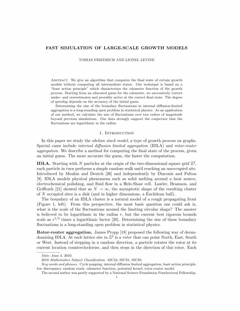
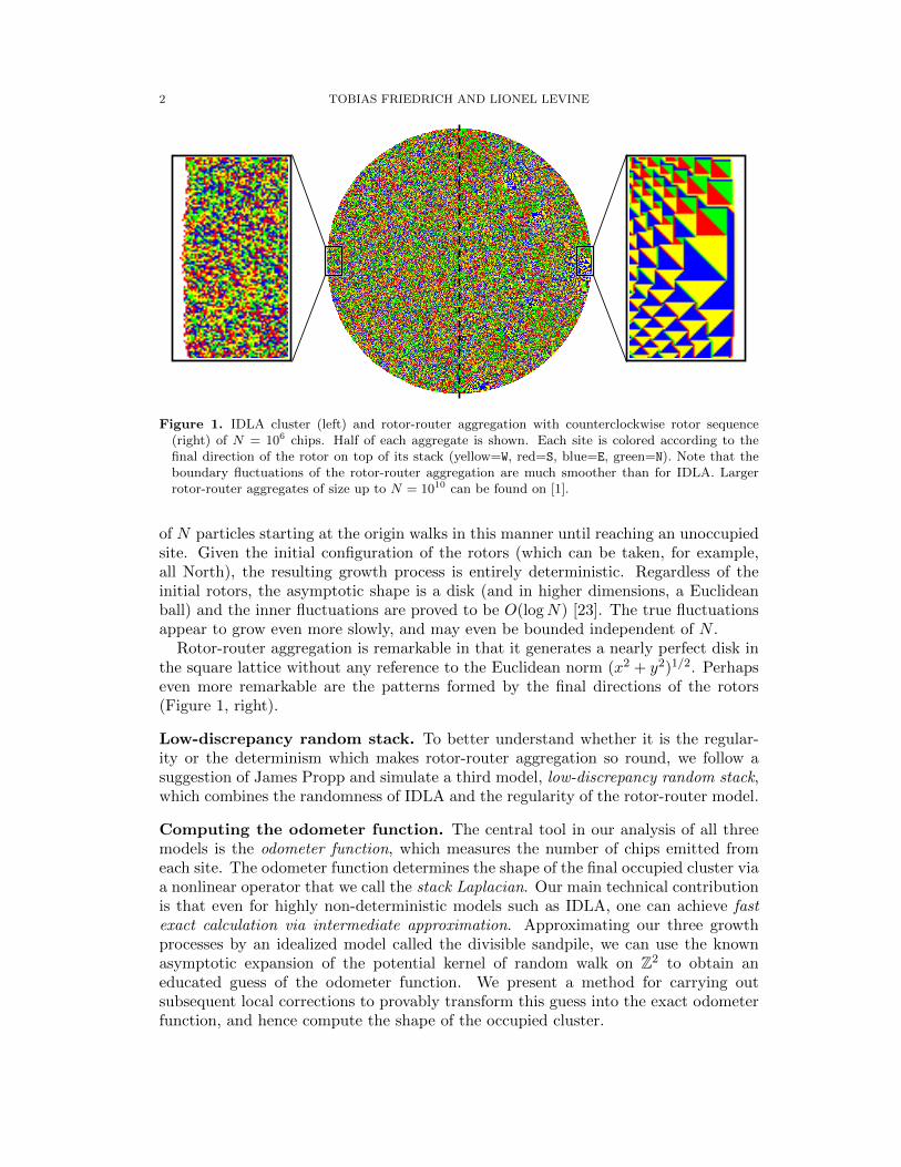
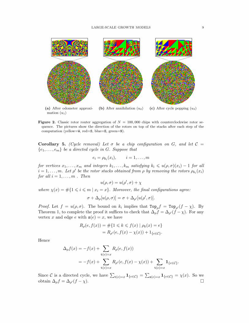
Figure 2. Classic rotor router aggregation of N = 100, 000 chips with counterclockwise rotor se-quence. The pictures show the direction of the rotors on top of the stacks after each step of thecomputation (yellow=W, red=S, blue=E, green=N).
Corollary 5. (Cycle removal) Let σ be a chip configuration on G, and let C =e1, . . . , em be a directed cycle in G. Suppose that
ei = ρki(xi), i = 1, . . . ,m
for vertices x1, . . . , xm and integers k1, . . . , km satisfying ki 6 u(ρ, σ)(xi) − 1 for alli = 1, . . . ,m. Let ρ′ be the rotor stacks obtained from ρ by removing the rotors ρki(xi)for all i = 1, . . . ,m . Then
u(ρ, σ) = u(ρ′, σ) + χ
where χ(x) = #1 6 i 6 m | xi = x. Moreover, the final configurations agree:
σ + ∆ρ[u(ρ, σ)] = σ + ∆ρ′ [u(ρ′, σ)].
Proof. Let f = u(ρ, σ). The bound on ki implies that Topρf = Topρ′(f − χ). By
Theorem 1, to complete the proof it suffices to check that ∆ρf = ∆ρ′(f −χ). For anyvertex x and edge e with s(e) = x, we have
Rρ(e, f(x)) = #1 6 k 6 f(x) | ρk(x) = e= Rρ′(e, f(x)− χ(x)) + 1e∈C.
Hence
∆ρf(x) = −f(x) +∑
t(e)=x
Rρ(e, f(x))
= −f(x) +∑
t(e)=x
Rρ′(e, f(x)− χ(x)) +∑
t(e)=x
1e∈C.
Since C is a directed cycle, we have∑
t(e)=x 1e∈C =∑
s(e)=x 1e∈C = χ(x). So we
obtain ∆ρf = ∆ρ′(f − χ).
10 TOBIAS FRIEDRICH AND LIONEL LEVINE
4. The Algorithm: From Approximation to Exact Calculation
In this section we describe how to compute the odometer function u exactly, givenas input an approximation u1. The running time depends on the accuracy of theapproximation, but the correctness of the output does not. In the next section weexplain how to find a good approximation u1 for the example of N chips started atthe origin in Z2.
We assume that G is strongly connected (finite or infinite), and that the initialconfiguration σ0 satisfies σ0(x) > 0 for all x, and
∑x σ0(x) < ∞. If G is finite, we
assume that∑
x σ0(x) is at most the number of vertices of G (otherwise, some chipswould never get absorbed). The only assumption on the approximation u1 is that it isnonnegative with finite support. Finally, we assume that the rotor stacks are infinitive,which ensures that the growth process terminates after finitely many firings: that is,∑
x∈V u(x) <∞.For x ∈ V , write
dout(x) = #e ∈ E | s(e) = xdin(x) = #e ∈ E | t(e) = x
for the out-degree and in-degree of x.The odometer function u depends on the initial chip configuration σ0 and on the
rotor stacks ρk(x). The latter are completely specified by the function R(e, n) definedin §3. Note that for rotor-router aggregation, since the stacks are periodic, R(e, n) hasthe simple explicit form
R(e, n) =
⌊n+ dout(x)− j
dout(x)
⌋(7)
where j is the least positive integer such that ρj(x) = e. For IDLA, R(e, n) is a randomvariable with the Binomial(n, p) distribution, where p is the transition probabilityassociated to the edge e.
In this section we take R(e, n) as known. From a computational standpoint, if thestacks are random, then determining R(e, n) involves calls to a pseudorandom numbergenerator. We address the issue of minimizing the number of such calls in §6.2.
Our algorithm consists of an approximation step followed by two error-correctionsteps: an annihilation step that corrects the chip locations, and a reverse cycle-poppingstep that corrects the rotors.
(1) Approximation. Perform firings according to the approximate odometer,by computing the chip configuration σ1 = σ0 + ∆ρu1. Using equation (3), thistakes time O(din(x) + 1) for each vertex x, for a total time of O(#E + #V ).This step is where the speedup occurs, because we are performing manyfirings at once:
∑x u1(x) is typically much larger than #E + #V . Output σ1.
(2) Annihilation. Start with u2 = u1 and σ2 = σ1. If x ∈ V satisfies σ2(x) > 1,then we call x a hill. If σ2(x) < 0, or if σ2(x) = 0 and u2(x) > 0, then we callx a hole. For each x ∈ Z2,(a) If x is a hill, fire it by incrementing u2(x) by one and then moving one
chip from x to t(Top(u2)(x)).(b) If x is a hole, unfire it by moving one chip from t(Top(u2)(x)) to x and
then decrementing u2(x) by one.
LARGE-SCALE GROWTH MODELS 11
(a) After odometer approxi-mation (σ1)
(b) After annihilation (σ2) (c) After cycle popping (σ3)
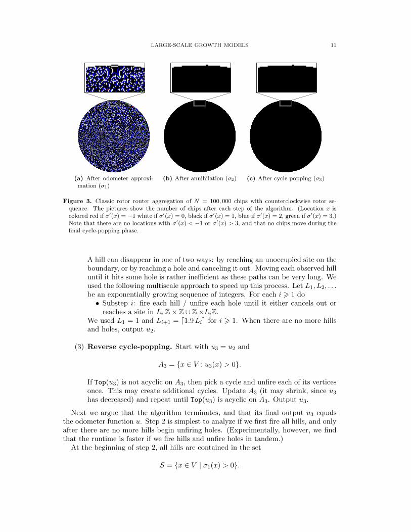
Figure 3. Classic rotor router aggregation of N = 100, 000 chips with counterclockwise rotor se-quence. The pictures show the number of chips after each step of the algorithm. (Location x iscolored red if σ′(x) = −1 white if σ′(x) = 0, black if σ′(x) = 1, blue if σ′(x) = 2, green if σ′(x) = 3.)Note that there are no locations with σ′(x) < −1 or σ′(x) > 3, and that no chips move during thefinal cycle-popping phase.
A hill can disappear in one of two ways: by reaching an unoccupied site on theboundary, or by reaching a hole and canceling it out. Moving each observed hilluntil it hits some hole is rather inefficient as these paths can be very long. Weused the following multiscale approach to speed up this process. Let L1, L2, . . .be an exponentially growing sequence of integers. For each i > 1 do• Substep i: fire each hill / unfire each hole until it either cancels out or
reaches a site in Li Z× Z ∪ Z×LiZ.We used L1 = 1 and Li+1 = d1.9Lie for i > 1. When there are no more hillsand holes, output u2.
(3) Reverse cycle-popping. Start with u3 = u2 and
A3 = x ∈ V : u3(x) > 0.
If Top(u3) is not acyclic on A3, then pick a cycle and unfire each of its verticesonce. This may create additional cycles. Update A3 (it may shrink, since u3has decreased) and repeat until Top(u3) is acyclic on A3. Output u3.
Next we argue that the algorithm terminates, and that its final output u3 equalsthe odometer function u. Step 2 is simplest to analyze if we first fire all hills, and onlyafter there are no more hills begin unfiring holes. (Experimentally, however, we findthat the runtime is faster if we fire hills and unfire holes in tandem.)
At the beginning of step 2, all hills are contained in the set
S = x ∈ V | σ1(x) > 0.
12 TOBIAS FRIEDRICH AND LIONEL LEVINE
Since σ0 and u1 have finite support, σ1 = σ0 + ∆ρu1 has finite support, so S is finite.Since the total number of chips is conserved, we have∑
x∈Vσ1(x) =
∑x∈V
σ0(x).
The right side is 6 #V by assumption. Therefore if S = V , we must have σ1(x) = 1for all x ∈ V ; in this case there are no hills or holes, and we move on to step 3.
Suppose now that S is a proper subset of V . Let
h =∑x∈S
(σ1(x)− 1)
be the total height of the hills. Note that firing a hill cannot increase h. If a givenvertex fires infinitely often, then since the rotor stacks are infinitive, each of its out-neighbors also fires infinitely often; since G is strongly connected, it would followthat every vertex fires infinitely often. Thus after firing finitely many hills, a chipmust leave S. When this happens, h decreases. Thus after finitely many firings wereach h = 0 and there are no more hills.
Next we begin unfiring the holes. After all hills have been settled, we have u2(x) > 0for all x ∈ V . The sum
∑x∈V u2(x) is finite, and each unfiring decreases it by one.
To show that the unfiring step terminates, it suffices to show that for all x ∈ Vthe unfiring of holes never causes u2(x) to become negative. Indeed, suppose thatu2(x) = 0 and u2(y) > 0 for all neighbors y of x. Then the number of chips at x isσ0(x) + ∆ρu2(x) > 0, so x is not a hole. Therefore the unfiring step terminates andits output u2 is nonnegative.
After step 2 there are no hills or holes, i.e., 0 6 σ2(x) 6 1 for all x, and if σ2(x) = 0then u2(x) = 0.
During step 3, we only unfire sites within A3. Since∑
x∈V u3(x) is finite anddecreases with each unfiring, this step terminates and its output u3 is nonnegative.When a cycle is unfired, each vertex in the cycle sends a chip to the previous vertex,so there is no net movement of chips: σ3 = σ2. In particular, there are no hills at theend of step 3. If σ3(x) = 0, then σ2(x) = 0; since there were no holes at the end ofstep 2, this means that u2(x) = 0, and hence u3(x) = 0. So there are still no holes atthe end of step 3. By construction, Top(u3) is acyclic on A3. Therefore all condtionsof Theorem 1 are satisified, which shows that u3 = u as desired.
5. Approximating the Odometer Function
Next we describe how to find a good approximation to the odometer to use as inputto the algorithm described in §4. Our main assumption will be that the rotor stacksare balanced in the sense that
R(e, n) ≈ R(e′, n)
for all n ∈ N and all edges e, e′ with s(e) = s(e′). By definition, rotor-router aggrega-tion obeys the strong balance condition
|R(e, n)−R(e′, n)| 6 1.
IDLA is somewhat less balanced: |R(e, n)− R(e′, n)| is typically on the order of√n.
It turns out that this level of balance is still enough to get a fairly good approximationand hence a significant speedup in our algorithm.
LARGE-SCALE GROWTH MODELS 13
If the rotor stacks are balanced, then the stack Laplacian ∆ρ is well-approximatedby the operator ∆ on functions u : V → Z defined by
∆u(z) =∑
t(e)=z
u(s(e))
dout(s(e))− u(z).
Note that ∆ is the adjoint of the usual discrete Laplacian on G.In this setting we can approximate the behavior of our stack-based aggregation with
an idealized model called the divisible sandpile [23]. Instead of discrete chips, eachvertex z has a real-valued “mass” σ0(z). Any site with mass greater than 1 can fireby keeping mass 1 for itself, and distributing the excess mass to its out-neighbors bysending an equal amount of mass along each outgoing edge. The resulting odometerfunction
v(z) = total mass emitted from z
satisfies the discrete variational problem
v > 0
∆v 6 1− σ0 (8)
v(∆v − 1 + σ0) = 0.
In words, these conditions say that each site emits a nonnegative amount of mass,each site ends with mass at most 1; and each site that emits a positive amount ofmass ends with mass exactly 1. The conditions (8) can be reformulated as an obstacleproblem, that of finding the smallest superharmonic function lying above a givenfunction; see [24]. That formulation shows existence and uniqueness of the solution v.
If the rotor stacks are sufficiently balanced, we expect the divisible sandpile odome-ter function v to approximate closely our abelian stack odometer u. The next questionis how to compute or approximate v. The obstacle problem formulation shows that vcan be computed exactly by linear programming. Such an approach works well forsmall to moderate system sizes, but for the sizes we are interested in, the number ofvariables v(z) is prohibitively large.
Fortunately, for specific examples it is sometimes possible to guess a near solu-tion w ≈ v. We briefly indicate how to do this for the specific example of interest tous, the initial configuration
σ0 = Nδo
consisting of N chips at the origin o ∈ Z2. In that case the set of sites that are fullyoccupied in the final divisible sandpile configuration σ0 + ∆v is very close to the disk
Br = z ∈ Z2 : |z| < rof radius r =
√N/π; see [23, Theorem 3.3]. Here |z| = (z21 + z22)1/2 is the Euclidean
norm. Thus we are seeking a function w : Z2 → R satisfying
∆w = 1−Nδo in Br
w ≈ 0 on ∂Br.
An example of such a function is
w(z) = |z|2 −Na(z)− r2 +Na((r, 0)) (9)
14 TOBIAS FRIEDRICH AND LIONEL LEVINE
where a(z) is the potential kernel for simple random walk (Xn)n>0 started at the originin Z2, defined as
a(z) =
∞∑n=1
(P(Xn = o)− P(Xn = z)) .
Its discrete Laplacian is ∆a = δo.As input to our algorithm we will use the function
w(z)+ := max(0, w(z))
where w(z) is given by (9). One computational issue remains, which is how to computethe potential kernel a(z). The potential kernel has the asymptotic expansion [14,Remark 2]
a(z) =2
πln |z|+ κ+
1
6π
8ω21ω
22 − 1
|z|2 +O(|z|−4) (10)
where ω = z/|z|, and κ = ln 8+2γπ ; here γ ≈ 0.577216 is Euler’s constant lim(
∑nk=1
1k −
lnn). Note that if θ is the argument of z, then
8ω21ω
22 − 1 = 8 sin2 θ cos2 θ − 1
= 2 sin2 2θ − 1
= sin2 2θ − cos2 2θ
= − cos 4θ.
Thus, identifying Z2 with Z + iZ ⊂ C, we can write
a(z) =2
πln |z|+ κ− 1
6π
Re(z4)
|z|6 +O(|z|−4).
For z close to the origin the error term O(|z|−4) becomes significant. Therefore, weuse the McCrea-Whipple algorithm [25] (see also [19]) to precompute a(z) exactly for|z| < 100. This algorithm uses the exact identity
a(n+ in) =4
π
n∑k=1
1
2k − 1
for n > 0, together with the relation ∆a = δo and reflection symmetry across the realand imaginary axes to compute a(z) recursively. As this calculation is numerically veryill-conditioned, we performed it in advance by symbolic calculation with a computeralgebra system.
Now we can describe the function u1 that we used as input to the first step of ouralgorithm. Let r =
√N/π. Approximating the term a((r, 0)) in (9) by 2
π log r+ κ, weset
u1(z) =⌊|z|2 + r2 (2 ln r − 1 + πκ− πa(z))
⌉, |z| < 100.
Here bte =⌊t+ 1
2
⌋denotes the closest integer to t ∈ R. For |z| > 100 we use the
asymptotic expansion for a(z) in (9), which gives
u1(z) =
⌊|z|2 + r2
(2 ln
r
|z| − 1 +Re(z4)
6 |z|6)⌉+
, |z| > 100,
where t+ := max(t, 0). Including more terms of the asymptotic expansion of a(z)from [19] improves the approximation very slightly, but increases the overall runtime.
LARGE-SCALE GROWTH MODELS 15
(a) N = 100000. (b) N = 100100. (c) N = 100200.
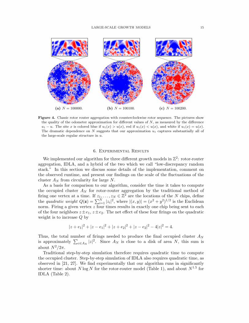
Figure 4. Classic rotor router aggregation with counterclockwise rotor sequence. The pictures showthe quality of the odometer approximation for different values of N , as measured by the differenceu1 − u. The site x is colored blue if u1(x) > u(x), red if u1(x) < u(x), and white if u1(x) = u(x).The dramatic dependence on N suggests that our approximation u1 captures substantially all ofthe large-scale regular structure in u.
6. Experimental Results
We implemented our algorithm for three different growth models in Z2: rotor-routeraggregation, IDLA, and a hybrid of the two which we call “low-discrepancy randomstack.” In this section we discuss some details of the implementation, comment onthe observed runtime, and present our findings on the scale of the fluctuations of thecluster AN from circularity for large N .
As a basis for comparison to our algorithm, consider the time it takes to computethe occupied cluster AN for rotor-router aggregation by the traditional method offiring one vertex at a time. If z1, . . . , zN ∈ Z2 are the locations of the N chips, definethe quadratic weight Q(z) =
∑Ni=1 |zi|2, where |(x, y)| = (x2 + y2)1/2 is the Euclidean
norm. Firing a given vertex z four times results in exactly one chip being sent to eachof the four neighbors z±e1, z±e2. The net effect of these four firings on the quadraticweight is to increase Q by
|z + e1|2 + |z − e1|2 + |z + e2|2 + |z − e2|2 − 4|z|2 = 4.
Thus, the total number of firings needed to produce the final occupied cluster ANis approximately
∑z∈AN
|z|2. Since AN is close to a disk of area N , this sum is
about N2/2π.Traditional step-by-step simulation therefore requires quadratic time to compute
the occupied cluster. Step-by-step simulation of IDLA also requires quadratic time, asobserved in [21, 27]. We find experimentally that our algorithm runs in significantlyshorter time: about N logN for the rotor-router model (Table 1), and about N1.5 forIDLA (Table 2).
16 TOBIAS FRIEDRICH AND LIONEL LEVINE
(a) N = 100000. (b) N = 100100. (c) N = 100200.
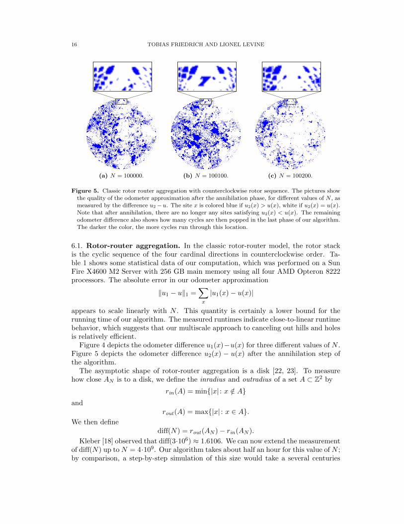
Figure 5. Classic rotor router aggregation with counterclockwise rotor sequence. The pictures showthe quality of the odometer approximation after the annihilation phase, for different values of N , asmeasured by the difference u2−u. The site x is colored blue if u2(x) > u(x), white if u2(x) = u(x).Note that after annihilation, there are no longer any sites satisfying u2(x) < u(x). The remainingodometer difference also shows how many cycles are then popped in the last phase of our algorithm.The darker the color, the more cycles run through this location.
6.1. Rotor-router aggregation. In the classic rotor-router model, the rotor stackis the cyclic sequence of the four cardinal directions in counterclockwise order. Ta-ble 1 shows some statistical data of our computation, which was performed on a SunFire X4600 M2 Server with 256 GB main memory using all four AMD Opteron 8222processors. The absolute error in our odometer approximation
‖u1 − u‖1 =∑x
|u1(x)− u(x)|
appears to scale linearly with N . This quantity is certainly a lower bound for therunning time of our algorithm. The measured runtimes indicate close-to-linear runtimebehavior, which suggests that our multiscale approach to canceling out hills and holesis relatively efficient.
Figure 4 depicts the odometer difference u1(x)−u(x) for three different values of N .Figure 5 depicts the odometer difference u2(x) − u(x) after the annihilation step ofthe algorithm.
The asymptotic shape of rotor-router aggregation is a disk [22, 23]. To measurehow close AN is to a disk, we define the inradius and outradius of a set A ⊂ Z2 by
rin(A) = min|x| : x /∈ Aand
rout(A) = max|x| : x ∈ A.We then define
diff(N) = rout(AN )− rin(AN ).
Kleber [18] observed that diff(3·106) ≈ 1.6106. We can now extend the measurementof diff(N) up to N = 4·109. Our algorithm takes about half an hour for this value of N ;by comparison, a step-by-step simulation of this size would take a several centuries
LARGE-SCALE GROWTH MODELS 17
Number ofRuntime
Radius Difference ‖u1− u‖1/N max |u1− u| highest deepest
chips N absolute recentered hill hole
210=1,024 1.29 ms 1.324 0.278 1.800 6 3 -1211=2,048 0.82 ms 1.490 0.273 1.142 5 3 -1212=4,096 1.69 ms 1.523 0.138 3.370 10 3 -1213=8,192 2.83 ms 1.606 0.235 3.599 11 3 -1214=16,384 5.03 ms 1.579 0.166 2.417 12 3 -1215=32,768 9.28 ms 1.567 0.274 2.405 10 3 -1216=65,536 24.0 ms 1.611 0.429 4.461 17 3 -1217=131,072 41.8 ms 1.652 0.279 2.486 16 3 -1218=262,144 80.8 ms 1.565 0.346 2.919 16 3 -1219=524,288 0.18 sec 1.463 0.237 2.955 16 3 -1220=1,048,576 0.40 sec 1.642 0.362 4.323 23 3 -1221=2,097,152 0.83 sec 1.591 0.297 3.594 26 3 -1222=4,194,304 1.72 sec 1.596 0.316 4.220 29 3 -1223=8,388,608 2.81 sec 1.674 0.418 3.141 34 3 -1224=16,777,216 5.85 sec 1.614 0.396 3.974 45 3 -1225=33,554,432 0.20 min 1.538 0.229 3.142 43 3 -1226=67,108,864 0.43 min 1.658 0.368 4.695 62 3 -1227=134,217,728 0.77 min 1.563 0.184 3.344 67 3 -1228=268,435,456 1.60 min 1.639 0.340 4.463 83 3 -1229=536,870,912 3.76 min 1.679 0.402 4.495 85 3 -1230=1,073,741,824 6.90 min 1.635 0.414 4.309 91 3 -1231=2,147,483,648 0.21 hours 1.521 0.304 3.932 127 3 -1232=4,294,967,296 0.50 hours 1.650 0.366 4.383 172 4 -2
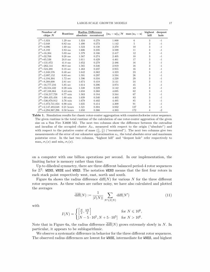
Table 1. Simulation results for classic rotor-router aggregation with counterclockwise rotor sequence.The given runtime is the total runtime of the calculation of one rotor-router aggreation of the givensize on a Sun Fire X4600 M2. The next two columns show the difference between the outradiusand inradius of the occupied cluster AN , measured with respect to the origin (“absolute”) andwith respect to the putative center of mass
(12, 12
)(“recentered”). The next two columns give two
measurements of the error of our odometer approximation u1, the total absolute error and maximumpointwise error. In the last two columns, “highest hill” and “deepest hole” refer respectively tomaxx σ1(x) and minx σ1(x).
on a computer with one billion operations per second. In our implementation, thelimiting factor is memory rather than time.
Up to dihedral symmetry, there are three different balanced period-4 rotor sequencesfor Z2: WENS, WNSE and WNES. The notation WENS means that the first four rotors ineach stack point respectively west, east, north and south.
Figure 6a shows the radius difference diff(N) for various N for the three differentrotor sequences. As these values are rather noisy, we have also calculated and plottedthe averages
diff(N) :=1
|I(N)|∑
N ′∈I(N)
diff(N ′) (11)
with
I(N) =
[N2 ,
3N2
]for N 6 106,
[N − 5 · 105, N + 5 · 105] for N > 106.
Note that in Figure 6a, the radius difference diff(N) grows extremely slowly in N . Inparticular, it appears to be sublogarithmic.
We observe a systematic difference in behavior for the three different rotor sequences.The observed radius differences are lowest for WNSE, intermediate for WNES, and highest
18 TOBIAS FRIEDRICH AND LIONEL LEVINE
0
0.2
0.4
0.6
0.8
1
1.2
1.4
1.6
1.8
2
100 101 102 103 104 105 106 107 108 109
in/outradiusdifferen
ce
number of chips N
WENS
WNES
WNSE
(a) Radius difference around the origin.
0
0.2
0.4
0.6
0.8
1
100 101 102 103 104 105 106 107 108 109
in/outradiusdifferen
ce
number of chips N
WNSEWENS
WNES
(b) Radius difference around putative center.
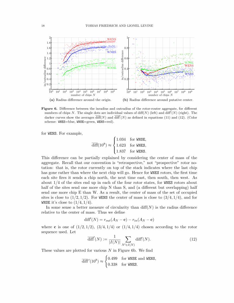
Figure 6. Difference between the inradius and outradius of the rotor-router aggregate, for differentnumbers of chips N . The single dots are individual values of diff(N) (left) and diff′(N) (right). The
darker curves show the averages diff(N) and diff′(N) as defined in equations (11) and (12). (Color
scheme: WNES=blue, WNSE=green, WENS=red).
for WENS. For example,
diff(108) ≈
1.034 for WNSE,
1.623 for WNES,
1.837 for WENS.
This difference can be partially explained by considering the center of mass of theaggregate. Recall that our convention is “retrospective,” not “prospective” rotor no-tation: that is, the rotor currently on top of the stack indicates where the last chiphas gone rather than where the next chip will go. Hence for WNES rotors, the first timeeach site fires it sends a chip north, the next time east, then south, then west. Asabout 1/4 of the sites end up in each of the four rotor states, for WNES rotors abouthalf of the sites send one more chip N than S, and (a different but overlapping) halfsend one more chip E than W. As a result, the center of mass of the set of occupiedsites is close to (1/2, 1/2). For WENS the center of mass is close to (3/4, 1/4), and forWNSE it’s close to (1/4, 1/4).
In some sense a better measure of circularity than diff(N) is the radius differencerelative to the center of mass. Thus we define
diff′(N) = rout(AN − c)− rin(AN − c)
where c is one of (1/2, 1/2), (3/4, 1/4) or (1/4, 1/4) chosen according to the rotorsequence used. Let
diff′(N) :=
1
|I(N)|∑
N ′∈I(N)
diff′(N). (12)
These values are plotted for various N in Figure 6b. We find
diff ′(108) ≈
0.499 for WNSE and WENS,
0.338 for WNES.
LARGE-SCALE GROWTH MODELS 19
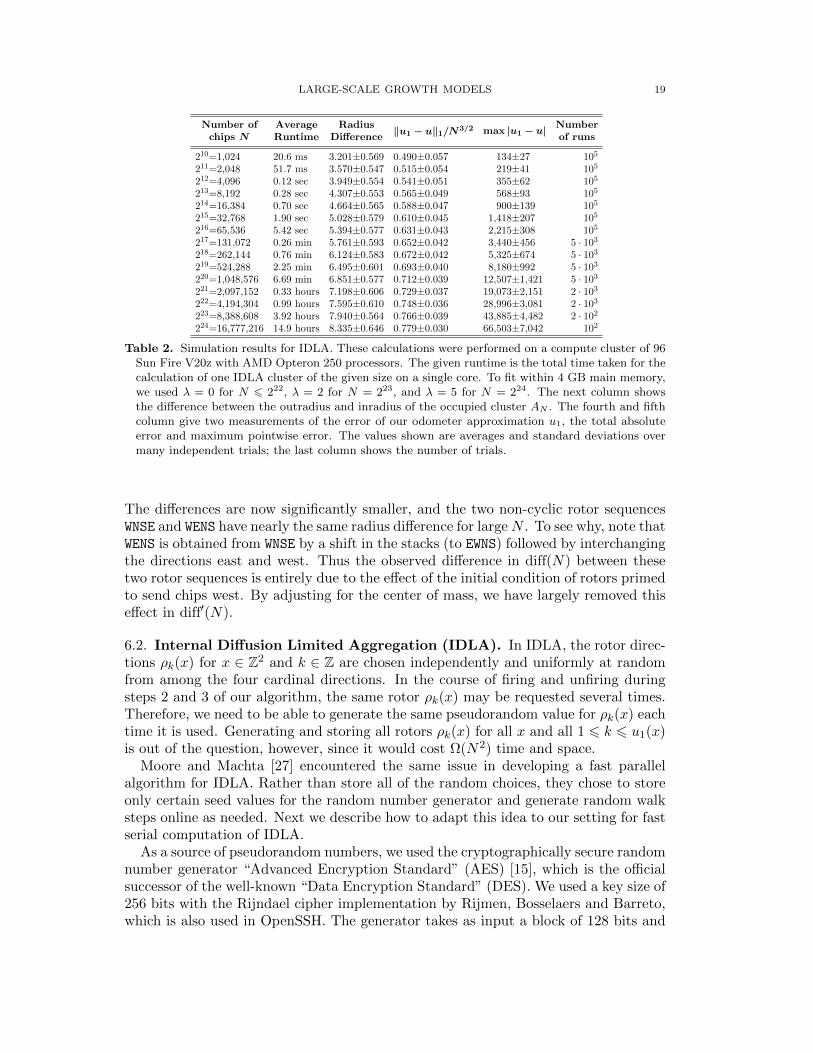
Number of Average Radius ‖u1− u‖1/N3/2 max |u1− u| Numberchips N Runtime Difference of runs
210=1,024 20.6 ms 3.201±0.569 0.490±0.057 134±27 105
211=2,048 51.7 ms 3.570±0.547 0.515±0.054 219±41 105
212=4,096 0.12 sec 3.949±0.554 0.541±0.051 355±62 105
213=8,192 0.28 sec 4.307±0.553 0.565±0.049 568±93 105
214=16,384 0.70 sec 4.664±0.565 0.588±0.047 900±139 105
215=32,768 1.90 sec 5.028±0.579 0.610±0.045 1,418±207 105
216=65,536 5.42 sec 5.394±0.577 0.631±0.043 2,215±308 105
217=131,072 0.26 min 5.761±0.593 0.652±0.042 3,440±456 5 · 103
218=262,144 0.76 min 6.124±0.583 0.672±0.042 5,325±674 5 · 103
219=524,288 2.25 min 6.495±0.601 0.693±0.040 8,180±992 5 · 103
220=1,048,576 6.69 min 6.851±0.577 0.712±0.039 12,507±1,421 5 · 103
221=2,097,152 0.33 hours 7.198±0.606 0.729±0.037 19,073±2,151 2 · 103
222=4,194,304 0.99 hours 7.595±0.610 0.748±0.036 28,996±3,081 2 · 103
223=8,388,608 3.92 hours 7.940±0.564 0.766±0.039 43,885±4,482 2 · 102
224=16,777,216 14.9 hours 8.335±0.646 0.779±0.030 66,503±7,042 102
Table 2. Simulation results for IDLA. These calculations were performed on a compute cluster of 96Sun Fire V20z with AMD Opteron 250 processors. The given runtime is the total time taken for thecalculation of one IDLA cluster of the given size on a single core. To fit within 4 GB main memory,we used λ = 0 for N 6 222, λ = 2 for N = 223, and λ = 5 for N = 224. The next column showsthe difference between the outradius and inradius of the occupied cluster AN . The fourth and fifthcolumn give two measurements of the error of our odometer approximation u1, the total absoluteerror and maximum pointwise error. The values shown are averages and standard deviations overmany independent trials; the last column shows the number of trials.
The differences are now significantly smaller, and the two non-cyclic rotor sequencesWNSE and WENS have nearly the same radius difference for largeN . To see why, note thatWENS is obtained from WNSE by a shift in the stacks (to EWNS) followed by interchangingthe directions east and west. Thus the observed difference in diff(N) between thesetwo rotor sequences is entirely due to the effect of the initial condition of rotors primedto send chips west. By adjusting for the center of mass, we have largely removed thiseffect in diff′(N).
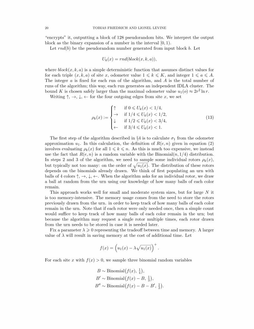
6.2. Internal Diffusion Limited Aggregation (IDLA). In IDLA, the rotor direc-tions ρk(x) for x ∈ Z2 and k ∈ Z are chosen independently and uniformly at randomfrom among the four cardinal directions. In the course of firing and unfiring duringsteps 2 and 3 of our algorithm, the same rotor ρk(x) may be requested several times.Therefore, we need to be able to generate the same pseudorandom value for ρk(x) eachtime it is used. Generating and storing all rotors ρk(x) for all x and all 1 6 k 6 u1(x)is out of the question, however, since it would cost Ω(N2) time and space.
Moore and Machta [27] encountered the same issue in developing a fast parallelalgorithm for IDLA. Rather than store all of the random choices, they chose to storeonly certain seed values for the random number generator and generate random walksteps online as needed. Next we describe how to adapt this idea to our setting for fastserial computation of IDLA.
As a source of pseudorandom numbers, we used the cryptographically secure randomnumber generator “Advanced Encryption Standard” (AES) [15], which is the officialsuccessor of the well-known “Data Encryption Standard” (DES). We used a key size of256 bits with the Rijndael cipher implementation by Rijmen, Bosselaers and Barreto,which is also used in OpenSSH. The generator takes as input a block of 128 bits and
20 TOBIAS FRIEDRICH AND LIONEL LEVINE
“encrypts” it, outputting a block of 128 pseudorandom bits. We interpret the outputblock as the binary expansion of a number in the interval [0, 1).
Let rnd(b) be the pseudorandom number generated from input block b. Let
Uk(x) = rnd(block(x, k, a)),
where block(x, k, a) is a simple deterministic function that assumes distinct values forfor each triple (x, k, a) of site x, odometer value 1 6 k 6 K, and integer 1 6 a 6 A.The integer a is fixed for each run of the algorithm, and A is the total number ofruns of the algorithm; this way, each run generates an independent IDLA cluster. Thebound K is chosen safely larger than the maximal odometer value u1(o) ≈ 2r2 ln r.
Writing ↑, →, ↓, ← for the four outgoing edges from site x, we set
ρk(x) :=
↑ if 0 6 Uk(x) < 1/4,
→ if 1/4 6 Uk(x) < 1/2,
↓ if 1/2 6 Uk(x) < 3/4,
← if 3/4 6 Uk(x) < 1.
(13)
The first step of the algorithm described in §4 is to calculate σ1 from the odometerapproximation u1. In this calculation, the definition of R(e, n) given in equation (2)involves evaluating ρk(x) for all 1 6 k 6 n. As this is much too expensive, we insteaduse the fact that R(e, n) is a random variable with the Binomial(n, 1/4) distribution.In steps 2 and 3 of the algorithm, we need to sample some individual rotors ρk(x),
but typically not too many: on the order of√u1(x). The distribution of these rotors
depends on the binomials already drawn. We think of first populating an urn withballs of 4 colors ↑,→, ↓,←. When the algorithm asks for an individual rotor, we drawa ball at random from the urn using our knowledge of how many balls of each colorremain.
This approach works well for small and moderate system sizes, but for large N itis too memory-intensive. The memory usage comes from the need to store the rotorspreviously drawn from the urn. in order to keep track of how many balls of each colorremain in the urn. Note that if each rotor were only needed once, then a simple countwould suffice to keep track of how many balls of each color remain in the urn; butbecause the algorithm may request a single rotor multiple times, each rotor drawnfrom the urn needs to be stored in case it is needed later.
Fix a parameter λ > 0 representing the tradeoff between time and memory. A largervalue of λ will result in saving memory at the cost of additional time. Let
f(x) =(u1(x)− λ
√u1(x)
)+.
For each site x with f(x) > 0, we sample three binomial random variables
B ∼ Binomial(f(x), 1
4
),
B′ ∼ Binomial(f(x)−B, 1
3
),
B′′ ∼ Binomial(f(x)−B −B′, 1
2
).

LARGE-SCALE GROWTH MODELS 21
0 10 20 30 40 50 60 70 80 90 1000
0.05
0.1
0.15
0.2
0.25 N = 210 N = 211 N = 212 N = 213
N = 214
N = 2151
2m + 2
moment m
variance
V
(a) Sample variance of the first 100 moments.
−2 −1 0 1 20
2000
4000
6000
8000
10000
12000
k=1
k=2
k=3
Re(Mm(AN ))/√N
frequen
cy
(b) Histograms of the first three moments.
Figure 7. Complex moments of the IDLA cluster. Left: The sample variance V (m) =
ERe(Mm(AN )/√N)2 of the real parts of the first 100 moments, for N = 210, . . . , 220. As N
increases, the variance of the real part of the m-th moment approaches 1/(2m + 2), in agreementwith the results of [17]. Right: Histogram of the real part of the first three moments for N = 216.The histogram shows 200,000 independent runs in bins of size 0.05. Data for the imaginary parts issimilar.
We then set
R(↑, f(x)) = B
R(→, f(x)) = B′
R(↓, f(x)) = B′′
R(←, f(x)) = f(x)−B −B′ −B′′.
Next, to implement step 1 of the algorithm described in §4, we need to knowR(e, u1(x)). So we compute
R(e, u1(x)) = R(e, f(x)) + #f(x) < k 6 u1(x) | ρk(x) = e.
Note that if λ is large, then this calculation is expensive in time, since it involvescalling the pseudorandom number generator to draw all of the rotors
ρk(x), f(x) < k 6 u1(x)
using equation (13). But, crucially, these rotors do not need to be stored.During steps 2 and 3 of the algorithm, we sample any rotors ρk(x) for k > f(x)
as needed using (13). Rotors ρk(x) for k 6 f(x) can be sampled online as needed
22 TOBIAS FRIEDRICH AND LIONEL LEVINE
0
1
2
3
4
5
6
7
8
9
20 22 24 26 28 210 212 214 216 218 220 222 224
number of chips N
in/outradiusdifferen
ce
(a) IDLA.
0
0.5
1
1.5
2
20 22 24 26 28 210 212 214 216 218 220 222 224 226 228
number of chips N
in/outradiusdifferen
ce
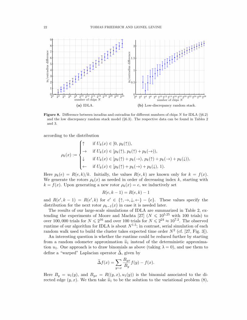
(b) Low-discrepancy random stack.
Figure 8. Difference between inradius and outradius for different numbers of chips N for IDLA (§6.2)and the low discrepancy random stack model (§6.3). The respective data can be found in Tables 2and 3.
according to the distribution
ρk(x) :=
↑ if Uk(x) ∈ [0, pk(↑)),→ if Uk(x) ∈ [pk(↑), pk(↑) + pk(→)),
↓ if Uk(x) ∈ [pk(↑) + pk(→), pk(↑) + pk(→) + pk(↓)),← if Uk(x) ∈ [pk(↑) + pk(→) + pk(↓), 1).
Here pk(e) = R(e, k)/k. Initially, the values R(e, k) are known only for k = f(x).We generate the rotors ρk(x) as needed in order of decreasing index k, starting withk = f(x). Upon generating a new rotor ρk(x) = e, we inductively set
R(e, k − 1) = R(e, k)− 1
and R(e′, k − 1) = R(e′, k) for e′ ∈ ↑,→, ↓,← − e. These values specify thedistribution for the next rotor ρk−1(x) in case it is needed later.
The results of our large-scale simulations of IDLA are summarized in Table 2, ex-tending the experiments of Moore and Machta [27] (N 6 105.25 with 100 trials) toover 100, 000 trials for N 6 216 and over 100 trials for N 6 224 ≈ 107.2. The observedruntime of our algorithm for IDLA is about N1.5; in contrast, serial simulation of eachrandom walk used to build the cluster takes expected time order N2 (cf. [27, Fig. 3]).
An interesting question is whether the runtime could be reduced further by startingfrom a random odometer approximation u1 instead of the deterministic approxima-tion u1. One approach is to draw binomials as above (taking λ = 0), and use them to
define a “warped” Laplacian operator ∆, given by
∆f(x) =∑y∼x
ByxBy
f(y)− f(x).
Here By = u1(y), and Byx = R((y, x), u1(y)) is the binomial associated to the di-rected edge (y, x). We then take u1 to be the solution to the variational problem (8),
LARGE-SCALE GROWTH MODELS 23
with ∆ replaced by ∆. This problem can be formulated as a linear program: minimize∑x u1(x) subject to the constraints u1 > 0 and ∆u1 6 1 − Nδo. One could even
iterate this construction, using u1 to draw new binomials and get a new warping˜∆,
and a new approximation ˜u1. A small number of iterations should suffice to bringthe approximation very close to the true odometer. The main computational issueis how to quickly solve (or even approximately solve) these linear programs, whichare sparse but quite large: the number of variables is about N . We achieved somemodest speedup with this kind of approach, but not enough to justify the additionalcomplexity.
To measure the circularity of the IDLA cluster, we computed the complex moments
Mm(AN ) =∑z∈AN
(zr
)mfor m = 1, . . . , 100. Here r =
√N/π, and we view z ∈ AN as a point in the complex
plane by identifying Z2 with Z+ iZ. These moments obey a central limit theorem [17]:
Mm(AN )/√N converges in distribution as N →∞ to a complex Gaussian with vari-
ance 1/(m+1). The distribution of the real part of Mm(AN )/√N is shown in Figure 7.
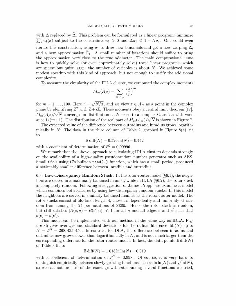
The expected value of the difference between outradius and inradius grows logarith-mically in N : The data in the third column of Table 2, graphed in Figure 8(a), fitto
Ediff(N) = 0.526 ln(N)− 0.442
with a coefficient of determination of R2 = 0.99996.We remark that the above approach to calculating IDLA clusters depends strongly
on the availability of a high-quality pseudorandom number generator such as AES.Small trials using C’s built-in rand( · ) function, which has a small period, produceda noticeably smaller difference between inradius and outradius.
6.3. Low-Discrepancy Random Stack. In the rotor-router model (§6.1), the neigh-bors are served in a maximally balanced manner, while in IDLA (§6.2), the rotor stackis completely random. Following a suggestion of James Propp, we examine a modelwhich combines both features by using low-discrepancy random stacks. In this modelthe neighbors are served in similarly balanced manner as the rotor-router model. Therotor stacks consist of blocks of length 4, chosen independently and uniformly at ran-dom from among the 24 permutations of NESW. Hence the rotor stack is random,but still satisfies |R(e, n) − R(e′, n)| 6 1 for all n and all edges e and e′ such thats(e) = s(e′).
This model can be implemented with our method in the same way as IDLA. Fig-ure 8b gives averages and standard deviations for the radius difference diff(N) up toN = 228 = 268, 435, 456. In contrast to IDLA, the difference between inradius andoutradius now grows slower than logarithmically in N , and is not much larger than thecorresponding difference for the rotor-router model. In fact, the data points Ediff(N)of Table 3 fit to
Ediff(N) = 1.018 ln ln(N)− 0.919
with a coefficient of determination of R2 = 0.998. Of course, it is very hard todistinguish empirically between slowly growing functions such as ln ln(N) and
√ln(N),
so we can not be sure of the exact growth rate; among several functions we tried,
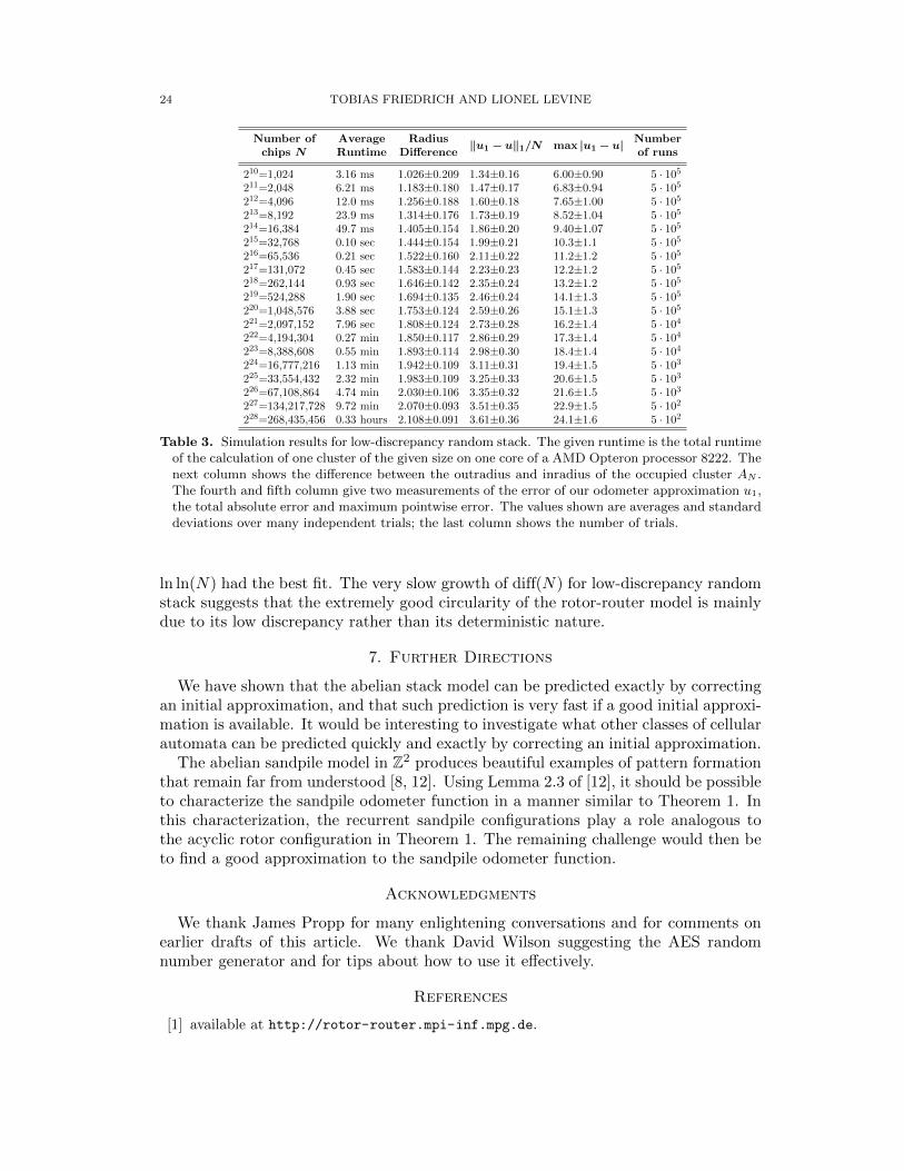
24 TOBIAS FRIEDRICH AND LIONEL LEVINE
Number of Average Radius ‖u1− u‖1/N max |u1− u| Numberchips N Runtime Difference of runs
210=1,024 3.16 ms 1.026±0.209 1.34±0.16 6.00±0.90 5 · 105
211=2,048 6.21 ms 1.183±0.180 1.47±0.17 6.83±0.94 5 · 105
212=4,096 12.0 ms 1.256±0.188 1.60±0.18 7.65±1.00 5 · 105
213=8,192 23.9 ms 1.314±0.176 1.73±0.19 8.52±1.04 5 · 105
214=16,384 49.7 ms 1.405±0.154 1.86±0.20 9.40±1.07 5 · 105
215=32,768 0.10 sec 1.444±0.154 1.99±0.21 10.3±1.1 5 · 105
216=65,536 0.21 sec 1.522±0.160 2.11±0.22 11.2±1.2 5 · 105
217=131,072 0.45 sec 1.583±0.144 2.23±0.23 12.2±1.2 5 · 105
218=262,144 0.93 sec 1.646±0.142 2.35±0.24 13.2±1.2 5 · 105
219=524,288 1.90 sec 1.694±0.135 2.46±0.24 14.1±1.3 5 · 105
220=1,048,576 3.88 sec 1.753±0.124 2.59±0.26 15.1±1.3 5 · 105
221=2,097,152 7.96 sec 1.808±0.124 2.73±0.28 16.2±1.4 5 · 104
222=4,194,304 0.27 min 1.850±0.117 2.86±0.29 17.3±1.4 5 · 104
223=8,388,608 0.55 min 1.893±0.114 2.98±0.30 18.4±1.4 5 · 104
224=16,777,216 1.13 min 1.942±0.109 3.11±0.31 19.4±1.5 5 · 103
225=33,554,432 2.32 min 1.983±0.109 3.25±0.33 20.6±1.5 5 · 103
226=67,108,864 4.74 min 2.030±0.106 3.35±0.32 21.6±1.5 5 · 103
227=134,217,728 9.72 min 2.070±0.093 3.51±0.35 22.9±1.5 5 · 102
228=268,435,456 0.33 hours 2.108±0.091 3.61±0.36 24.1±1.6 5 · 102
Table 3. Simulation results for low-discrepancy random stack. The given runtime is the total runtimeof the calculation of one cluster of the given size on one core of a AMD Opteron processor 8222. Thenext column shows the difference between the outradius and inradius of the occupied cluster AN .The fourth and fifth column give two measurements of the error of our odometer approximation u1,the total absolute error and maximum pointwise error. The values shown are averages and standarddeviations over many independent trials; the last column shows the number of trials.
ln ln(N) had the best fit. The very slow growth of diff(N) for low-discrepancy randomstack suggests that the extremely good circularity of the rotor-router model is mainlydue to its low discrepancy rather than its deterministic nature.
7. Further Directions
We have shown that the abelian stack model can be predicted exactly by correctingan initial approximation, and that such prediction is very fast if a good initial approxi-mation is available. It would be interesting to investigate what other classes of cellularautomata can be predicted quickly and exactly by correcting an initial approximation.
The abelian sandpile model in Z2 produces beautiful examples of pattern formationthat remain far from understood [8, 12]. Using Lemma 2.3 of [12], it should be possibleto characterize the sandpile odometer function in a manner similar to Theorem 1. Inthis characterization, the recurrent sandpile configurations play a role analogous tothe acyclic rotor configuration in Theorem 1. The remaining challenge would then beto find a good approximation to the sandpile odometer function.
Acknowledgments
We thank James Propp for many enlightening conversations and for comments onearlier drafts of this article. We thank David Wilson suggesting the AES randomnumber generator and for tips about how to use it effectively.
References
[1] available at http://rotor-router.mpi-inf.mpg.de.
LARGE-SCALE GROWTH MODELS 25
[2] P. Bak, C. Tang, and K. Wiesenfeld. Self-organized criticality: an explanation of the 1/fnoise. Phys. Rev. Lett., 59(4):381–384, 1987.
[3] R. D. Barve, E. F. Grove, and J. S. Vitter. Simple randomized mergesort on paralleldisks. Parallel Computing, 23(4-5):601–631, 1997.
[4] J. Cooper and J. Spencer. Simulating a random walk with constant error. Combinatorics,Probability & Computing, 15:815–822, 2006.
[5] J. Cooper, B. Doerr, J. Spencer, and G. Tardos. Deterministic random walks on theintegers. European Journal of Combinatorics, 28:2072–2090, 2007.
[6] J. Cooper, B. Doerr, T. Friedrich, and J. Spencer. Deterministic random walks on regulartrees. Random Structures and Algorithms, 2010+. To appear; Preliminary version ap-peared in 19th Annual ACM-SIAM Symposium on Discrete Algorithms (SODA’08), pages766–772, 2008.
[7] D. Dhar. Theoretical studies of self-organized criticality. Physica A, 369:29–70, 2006. Seealso arXiv:cond-mat/9909009.
[8] D. Dhar, T. Sadhu, and S. Chandra. Pattern formation in growing sandpiles. Europhys.Lett., 85, 2009. arXiv:0808.1732.
[9] P. Diaconis and W. Fulton. A growth model, a game, an algebra, Lagrange inversion, andcharacteristic classes. Rend. Sem. Mat. Univ. Politec. Torino, 49(1):95–119, 1991.
[10] B. Doerr and T. Friedrich. Deterministic random walks on the two-dimensional grid.Combinatorics, Probability & Computing, 18(1-2):123–144, 2009.
[11] B. Doerr, T. Friedrich, and T. Sauerwald. Quasirandom rumor spreading. In 19th AnnualACM-SIAM Symposium on Discrete Algorithms (SODA’08), pages 773–781, 2008.
[12] A. Fey, L. Levine, and Y. Peres. Growth rates and explosions in sandpiles. J. Stat. Phys.,138:143–159, 2010. arXiv:math/0901.3805.
[13] T. Friedrich, M. Gairing, and T. Sauerwald. Quasirandom load balancing. In 21st AnnualACM-SIAM Symposium on Discrete Algorithms (SODA’10), pages 1620–1629, 2010.
[14] Y. Fukai and K. Uchiyama. Potential kernel for two-dimensional random walk. Ann.Probab., 24(4):1979–1992, 1996.
[15] P. Hellekalek and S. Wegenkittl. Empirical evidence concerning AES. ACM Trans. Model.Comput. Simul., 13(4):322–333, 2003.
[16] A. E. Holroyd and J. Propp. Rotor walks and Markov chains. Algorithmic Probabilityand Combinatorics, 2010. To appear. arXiv:0904.4507.
[17] D. Jerison, L. Levine, and S. Sheffield. Internal DLA and the Gaussian free field, 2010.Manuscript in preparation.
[18] M. Kleber. Goldbug variations. Math. Intelligencer, 27(1):55–63, 2005.[19] G. Kozma and E. Schreiber. An asymptotic expansion for the discrete harmonic potential.
Electron. J. Probab., 9(1):1–17, 2004.[20] G. F. Lawler. Subdiffusive fluctuations for internal diffusion limited aggregation. Ann.
Probab., 23(1):71–86, 1995.[21] G. F. Lawler, M. Bramson, and D. Griffeath. Internal diffusion limited aggregation. Ann.
Probab., 20(4):2117–2140, 1992.[22] L. Levine and Y. Peres. Spherical asymptotics for the rotor-router model in Zd. Indiana
Univ. Math. J., 57(1):431–450, 2008.[23] L. Levine and Y. Peres. Strong spherical asymptotics for rotor-router aggregation and
the divisible sandpile. Potential Anal., 30:1–27, 2009.[24] L. Levine and Y. Peres. Scaling limits for internal aggregation models with multiple
sources. J. d’Analyse Math., 2010. To appear. arXiv:0712.3378.[25] W. H. McCrea and F. J. Whipple. Random paths in two and three dimensions. Proc.
Royal Soc., 60:281–298, 1940.[26] P. Meakin and J. M. Deutch. The formation of surfaces by diffusion-limited annihilation.
J. Chem. Phys., 85, 1986.
26 TOBIAS FRIEDRICH AND LIONEL LEVINE
[27] C. Moore and J. Machta. Internal diffusion-limited aggregation: parallel algorithms andcomplexity. J. Stat. Phys., 99(3-4):661–690, 2000.
[28] J. G. Propp and D. B. Wilson. How to get a perfectly random sample from a genericMarkov chain and generate a random spanning tree of a directed graph. J. Algorithms.,27:170–217, 1998.
[29] D. B. Wilson. Generating random spanning trees more quickly than the cover time. In28th Annual ACM Symposium on the Theory of Computing (STOC ’96), pages 296–303,1996.