FAST SOLVERS FOR OPTIMAL CONTROL … SOLVERS FOR OPTIMAL CONTROL PROBLEMS FROM PATTERN FORMATION MARTIN STOLL∗, JOHN W. PEARSON†, AND PHILIP K. MAINI‡ Abstract. The modelling

FAST SOLVERS FOR OPTIMAL CONTROL PROBLEMS FROM PATTERN

FORMATION

MARTIN STOLL∗, JOHN W. PEARSON† , AND PHILIP K. MAINI‡

Abstract. The modelling of pattern formation in biological systems using various models of reaction-diffusiontype has been an active research topic for many years. We here look at a parameter identification (or PDE-constrainedoptimization) problem where the Schnakenberg and Gierer-Meinhardt equations, two well-known pattern formationmodels, form the constraints to an objective function. Our main focus is on the efficient solution of the associatednonlinear programming problems via a Lagrange-Newton scheme. In particular we focus on the fast and robustsolution of the resulting large linear systems, which are of saddle point form. We illustrate this by considering severaltwo- and three-dimensional setups for both models. Additionally, we discuss an image-driven formulation that allowsus to identify parameters of the model to match an observed quantity obtained from an image.

Key words. PDE-constrained optimization, reaction-diffusion, pattern formation, Newton iteration, precondi-tioning, Schur complement.

AMS subject classifications. 65F08, 65F10, 65F50, 92-08, 93C20

1. Introduction. One of the fundamental problems in developmental biology is to understandhow spatial patterns, such as pigmentation patterns, skeletal structures, and so on, arise. In 1952,Alan Turing [36] proposed his theory of pattern formation in which he hypothesized that a system ofchemicals, reacting and diffusing, could be driven unstable by diffusion, leading to spatial patterns(solutions which are steady in time but vary in space). He proposed that these chemical patterns,which he termed morphogen patterns, set up pre-patterns which would then be interpreted by cellsin a concentration-dependent manner, leading to the patterns that we see.

These models have been applied to a very wide range of areas (see, for example, Murray [23])and have been shown to exist in chemistry [5, 26]. While their applicability to biology remainscontroversial, there are many examples which suggest that Turing systems may be underlying keypatterning processes (see [1, 7, 34] for the most recent examples). Two important models whichembody the essence of the original Turing model are the Gierer-Meinhardt [13] and Schnakenbergmodels [33] and it is upon these models which we focus.1 In light of the fact that to date, no Turingmorphogens have been unequivocally demonstrated, we do not have model parameter values so akey problem in mathematical biology is to determine parameters that give rise to certain observedpatterns. It is this problem that the present study investigates.

More recently, an area in applied and numerical mathematics that has generated much researchinterest is that of optimal control problems (see [35] for an excellent introduction to this field). Ithas been found that one key application of such optimal control formulations is to find solutions topattern formation problems [10, 11], and so it is natural to explore this particular application here.

∗Computational Methods in Systems and Control Theory, Max Planck Institute for Dynamics of Complex Tech-nical Systems, Sandtorstr. 1, 39106 Magdeburg, Germany ([email protected]),

†School of Mathematics, The University of Edinburgh, James Clerk Maxwell Building, The King’s Buildings,Mayfield Road, Edinburgh, EH9 3JZ, UK ([email protected]),

‡Wolfson Centre for Mathematical Biology, Mathematical Institute, University of Oxford, Radcliffe ObservatoryQuarter, Woodstock Road, Oxford, OX2 6GG, UK ([email protected])

1Although the second model is commonly referred to as the Schnakenberg model, it was actually first proposed byGierer and Meinhardt in [13] along with the model usually referenced as the Gierer-Meinhardt model – we thereforerefer to the first and second models as ‘GM1’ and ‘GM2’ within our working.

1

2 M. STOLL, J. W. PEARSON, AND P. K. MAINI

In this paper, we consider the numerical solution of optimal control (in this case parameteridentification) formulations of these Turing models – in particular we wish to devise preconditionediterative solvers for the matrix systems arising from the application of Newton and Gauss-Newtonmethods to the problems. The crucial aspect of the preconditioners is the utilization of saddle pointtheory to obtain effective approximations of the (1, 1)-block and Schur complement of these matrixsystems. The solvers will incorporate aspects of iterative solution strategies developed by the firstand second authors to tackle simpler optimal control problems in literature such as [28, 29, 30, 31].

This paper is structured as follows. In Section 2 we introduce the Gierer-Meinhardt (GM1)and Schnakenberg (GM2) models that we consider, and outline the corresponding optimal controlproblems. In Section 3 we discuss the outer (Newton-type) iteration that we employ for theseproblems, and state the resulting matrix systems at each iteration. We then motivate and deriveour preconditioning strategies in Section 4. In Section 5 we present numerical results to demonstratethe effectiveness of our approaches, and finally in Section 6 we make some concluding remarks.

2. A parameter identification problem. Parameter identification problems are crucial indetermining the setup of a mathematical model, often given by a system of differential equations,that is best suited to describe measured data or an observed phenomenon. These problems are oftenposed as PDE-constrained optimization problems [19, 35]. We here want to minimize an objectivefunction of misfit type, i.e., the function is designed to penalize deviations of the function valuesfrom the observed or measured data. The particular form is given by [13]

J(u, v, a, b) =β1

2‖u(x, t) − u(x, t)‖

2L2(Ω×[0,T ]) +

β2

2‖v(x, t) − v(x, t)‖

2L2(Ω×[0,T ]) (2.1)

+βT,1

2‖u(x, T ) − uT ‖

2L2(Ω) +

βT,2

2‖v(x, T ) − vT ‖

2L2(Ω)

+ν1

2‖a(x, t)‖

2L2(Ω×[0,T ]) +

ν2

2‖b(x, t)‖

2L2(Ω×[0,T ]) ,

where u, v are the state variables, and a, b the control variables, in our formulation. This is to saywe wish to ensure that the state variables are as close as possible in the L2-norm to some observedor desired states u, v, uT , vT , but at the same time penalize the enforcement of controls that havelarge magnitudes in this norm.

Our goal is to identify the parameters of classical pattern formation equations such that theresulting optimal parameters allow the use of these models for real-world data. We here use modelsof reaction-diffusion type typically exploited to generate patterns seen in biological systems. Thetwo formulations we consider are the GM1 model [13, 23]

ut −Du∆u−ru2

v+ au = r, on Ω × [0, T ], (2.2)

vt −Dv∆v − ru2 + bv = 0, on Ω × [0, T ],

u(x, 0) = u0(x), v(x, 0) = v0(x), on Ω,

∂u

∂ν=∂v

∂ν= 0, on ∂Ω × [0, T ],

FAST SOLVERS FOR PATTERN FORMATION 3

and the GM2 model [23, 33]

ut −Du∆u+ γ(u− u2v) − γa = 0, on Ω × [0, T ], (2.3)

vt −Dv∆v + γu2v − γb = 0, on Ω × [0, T ],

u(x, 0) = u0(x), v(x, 0) = v0(x), on Ω,

∂u

∂ν=∂v

∂ν= 0, on ∂Ω × [0, T ],

where r and γ are non-negative parameters involved in the respective models.

Both the GM1 and GM2 formulations are models of reaction-diffusion processes occurringin many types of pattern formation and morphogenesis processes [13, 23, 33]. The GM1 modelrelates to an “activator-inhibitor” system, whereas the GM2 model represents substrate-depletion.Within both models the variables u and v, the state variables in our formulation, represent theconcentrations of chemical products. The parameters Du and Dv denote the diffusion coefficients– typically it is assumed that v diffuses faster than u, so Du < Dv [13]. The parameters r and γ

are positive parameters: the value r in the GM1 model denotes the (small) production rate of theactivator [13], and the parameter γ in the GM2 model is the Hill coefficient, which describes thecooperativity within a binding process. The variables a and b, the control variables in our problem,represent the rates of decay for u and v, respectively.

Throughout the remainder of this article we will consider the minimization of the cost func-tional (2.1), with PDE constraints taking the form of the GM1 model or the GM2 model. PDE-constrained optimization problems of similar form have been considered in the literature, such asin [10, 11].

As the optimization problem min(u,v,a,b) J(u, v, a, b) subject to (2.2) or (2.3) is nonlinear dueto the nature of the constraints, we have to apply nonlinear programming [25] algorithms. Manyof these are generalizations of Newton’s method [25]. We here focus on a Lagrange-Newton (orbasic SQP) scheme and a Gauss-Newton method. At the heart of both approaches lies the solutionof large linear systems, which are often in saddle point form [3, 8], that represent the Hessian oran approximation to it. In order to be able to solve these large linear systems we need to employiterative solvers [8, 32], which can be accelerated using effective preconditioners.

3. Nonlinear programming. A standard way of how to proceed with the above nonlinearprogram is to consider a classical Lagrangian approach [35]. In our case with a nonlinear constraintwe apply a nonlinear solver to the first order conditions. Hence, we start by deriving the first orderconditions or Karush-Kuhn-Tucker conditions of the Lagrangian

L(u, v, a, b, p, q) = J(u, v, a, b) + (p,R1(u, v, a, b)) + (q,R2(u, v, a, b)) ,

where R1(u, v, a, b) and R2(u, v, a, b) represent the first two equations of both GM1 and GM2models. Note that for convenience our Lagrangian ignores the boundary and initial conditions. Ingeneral form the first order conditions are given by

Lu = 0, Lv = 0,La = 0, Lb = 0,Lp = 0, Lq = 0.


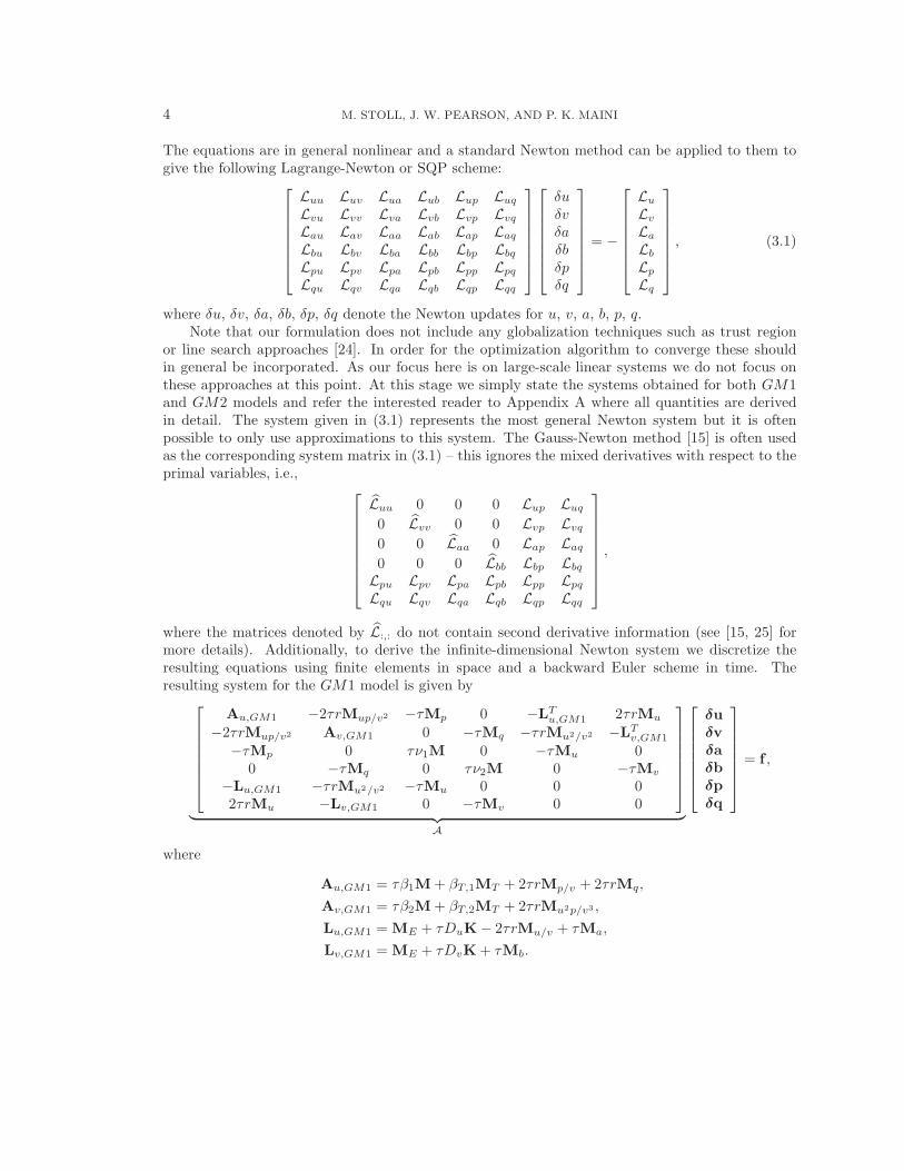
The equations are in general nonlinear and a standard Newton method can be applied to them togive the following Lagrange-Newton or SQP scheme:

Luu Luv Lua Lub Lup LuqLvu Lvv Lva Lvb Lvp LvqLau Lav Laa Lab Lap LaqLbu Lbv Lba Lbb Lbp LbqLpu Lpv Lpa Lpb Lpp LpqLqu Lqv Lqa Lqb Lqp Lqq

δu

δv

δa

δb

δp

δq

= −

LuLvLaLbLpLq

, (3.1)

where δu, δv, δa, δb, δp, δq denote the Newton updates for u, v, a, b, p, q.Note that our formulation does not include any globalization techniques such as trust region

or line search approaches [24]. In order for the optimization algorithm to converge these shouldin general be incorporated. As our focus here is on large-scale linear systems we do not focus onthese approaches at this point. At this stage we simply state the systems obtained for both GM1and GM2 models and refer the interested reader to Appendix A where all quantities are derivedin detail. The system given in (3.1) represents the most general Newton system but it is oftenpossible to only use approximations to this system. The Gauss-Newton method [15] is often usedas the corresponding system matrix in (3.1) – this ignores the mixed derivatives with respect to theprimal variables, i.e.,

Luu 0 0 0 Lup Luq0 Lvv 0 0 Lvp Lvq0 0 Laa 0 Lap Laq0 0 0 Lbb Lbp Lbq

Lpu Lpv Lpa Lpb Lpp LpqLqu Lqv Lqa Lqb Lqp Lqq

,

where the matrices denoted by L:,: do not contain second derivative information (see [15, 25] formore details). Additionally, to derive the infinite-dimensional Newton system we discretize theresulting equations using finite elements in space and a backward Euler scheme in time. Theresulting system for the GM1 model is given by

Au,GM1 −2τrMup/v2 −τMp 0 −LTu,GM1 2τrMu

−2τrMup/v2 Av,GM1 0 −τMq −τrMu2/v2 −LTv,GM1

−τMp 0 τν1M 0 −τMu 00 −τMq 0 τν2M 0 −τMv

−Lu,GM1 −τrMu2/v2 −τMu 0 0 02τrMu −Lv,GM1 0 −τMv 0 0

︸︷︷︸A

δu

δv

δa

δb

δp

δq

= f ,

where

Au,GM1 = τβ1M + βT,1MT + 2τrMp/v + 2τrMq,

Av,GM1 = τβ2M + βT,2MT + 2τrMu2p/v3 ,

Lu,GM1 = ME + τDuK− 2τrMu/v + τMa,

Lv,GM1 = ME + τDvK + τMb.


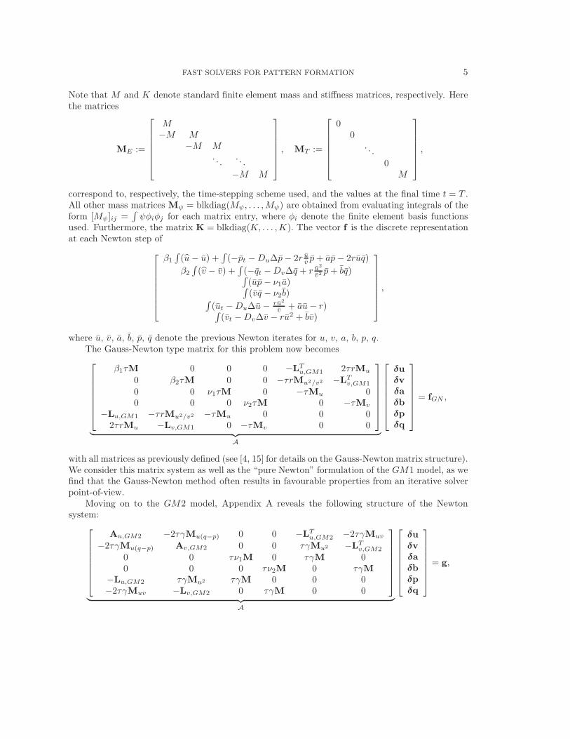
Note that M and K denote standard finite element mass and stiffness matrices, respectively. Herethe matrices

ME :=

M

−M M

−M M. . .

. . .

−M M

, MT :=

00

. . .

0M

,

correspond to, respectively, the time-stepping scheme used, and the values at the final time t = T .All other mass matrices Mψ = blkdiag(Mψ, . . . ,Mψ) are obtained from evaluating integrals of theform [Mψ]ij =

∫ψφiφj for each matrix entry, where φi denote the finite element basis functions

used. Furthermore, the matrix K = blkdiag(K, . . . ,K). The vector f is the discrete representationat each Newton step of

β1

∫(u − u) +

∫(−pt −Du∆p− 2r uv p+ ap− 2ruq)

β2

∫(v − v) +

∫(−qt −Dv∆q + r u

2

v2 p+ bq)∫(up− ν1a)∫(vq − ν2b)∫

(ut −Du∆u− ru2

v + au− r)∫(vt −Dv∆v − ru2 + bv)

,

where u, v, a, b, p, q denote the previous Newton iterates for u, v, a, b, p, q.The Gauss-Newton type matrix for this problem now becomes

β1τM 0 0 0 −LTu,GM1 2τrMu

0 β2τM 0 0 −τrMu2/v2 −LTv,GM1

0 0 ν1τM 0 −τMu 00 0 0 ν2τM 0 −τMv

−Lu,GM1 −τrMu2/v2 −τMu 0 0 02τrMu −Lv,GM1 0 −τMv 0 0

︸︷︷︸A

δu

δv

δa

δb

δp

δq

= fGN ,

with all matrices as previously defined (see [4, 15] for details on the Gauss-Newton matrix structure).We consider this matrix system as well as the “pure Newton” formulation of the GM1 model, as wefind that the Gauss-Newton method often results in favourable properties from an iterative solverpoint-of-view.

Moving on to the GM2 model, Appendix A reveals the following structure of the Newtonsystem:

Au,GM2 −2τγMu(q−p) 0 0 −LTu,GM2 −2τγMuv

−2τγMu(q−p) Av,GM2 0 0 τγMu2 −LTv,GM2

0 0 τν1M 0 τγM 00 0 0 τν2M 0 τγM

−Lu,GM2 τγMu2 τγM 0 0 0−2τγMuv −Lv,GM2 0 τγM 0 0

︸︷︷︸A

δu

δv

δa

δb

δp

δq

= g,


with

Au,GM2 = τβ1M + βT,1MT + 2τγMv(q−p),

Av,GM2 = τβ2M + βT,2MT ,

Lu,GM2 = ME + τDuK + τγM − 2γMuv,

Lv,GM2 = ME + τDvK + τγMu2 ,

and g the discrete representation of

β1

∫(u− u) +

∫(−pt −Du∆p+ 2γuv(q − p) + γp)

β2

∫(v − v) +

∫(−qt −Dv∆q + γu2(q − p))−

∫(ν1a+ γp)

−∫(ν2b+ γq)∫

(ut −Du∆u+ γ(u− u2v) − γa)∫(vt −Dv∆v + γu2v − γb)

.

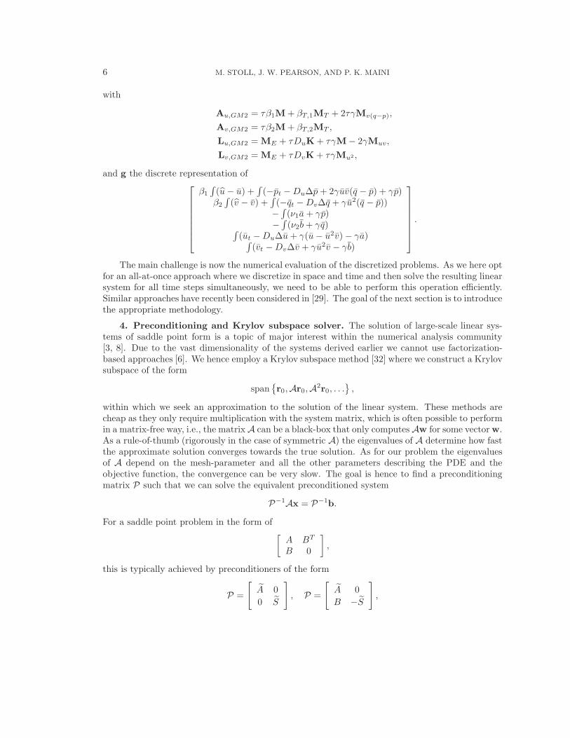
The main challenge is now the numerical evaluation of the discretized problems. As we here optfor an all-at-once approach where we discretize in space and time and then solve the resulting linearsystem for all time steps simultaneously, we need to be able to perform this operation efficiently.Similar approaches have recently been considered in [29]. The goal of the next section is to introducethe appropriate methodology.

4. Preconditioning and Krylov subspace solver. The solution of large-scale linear sys-tems of saddle point form is a topic of major interest within the numerical analysis community[3, 8]. Due to the vast dimensionality of the systems derived earlier we cannot use factorization-based approaches [6]. We hence employ a Krylov subspace method [32] where we construct a Krylovsubspace of the form

spanr0,Ar0,A

2r0, . . .,

within which we seek an approximation to the solution of the linear system. These methods arecheap as they only require multiplication with the system matrix, which is often possible to performin a matrix-free way, i.e., the matrix A can be a black-box that only computes Aw for some vector w.As a rule-of-thumb (rigorously in the case of symmetric A) the eigenvalues of A determine how fastthe approximate solution converges towards the true solution. As for our problem the eigenvaluesof A depend on the mesh-parameter and all the other parameters describing the PDE and theobjective function, the convergence can be very slow. The goal is hence to find a preconditioningmatrix P such that we can solve the equivalent preconditioned system

P−1Ax = P−1b.

For a saddle point problem in the form of[A BT

B 0

],

this is typically achieved by preconditioners of the form

P =

[A 0

0 S

], P =

[A 0

B −S

],


where A approximates the (1, 1)-block of the saddle point matrix A and S approximates the (neg-ative) Schur complement BA−1BT . This is motivated by results obtained in [20, 22] where it is

shown that the exact preconditioners A = A and S = BA−1BT lead to a very small number ofeigenvalues and hence iteration numbers. The choice of the outer Krylov subspace solver typicallydepends on the nature of the system matrix and the preconditioner. For symmetric indefinitesystems such as the ones presented here we usually choose Minres [27] based on a three-term re-currence relation. However as Minres typically needs a symmetric positive definite preconditioner,in the case of an indefinite preconditioner P we cannot use this method. We then need to apply anonsymmetric solver of which there exist many, and it is not obvious which of them is best suitedto any particular problem. Our rule-of-thumb is that if one carefully designs a preconditioner suchthat the eigenvalues of the preconditioned system are tightly clustered (or are contained within asmall number of clusters), many different solvers perform in a fairly similar way. For simplicity wehere choose Bicg [9], which is the extension of cg [16] to nonsymmetric problems and is based onthe nonsymmetric Lanczos process [14].

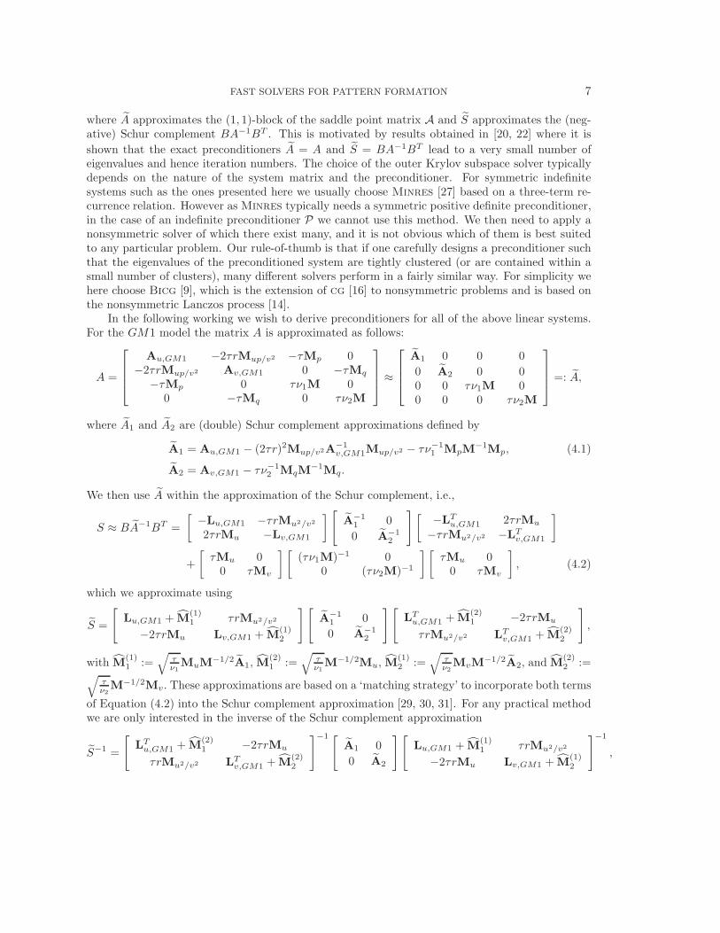
In the following working we wish to derive preconditioners for all of the above linear systems.For the GM1 model the matrix A is approximated as follows:

A =

Au,GM1 −2τrMup/v2 −τMp 0−2τrMup/v2 Av,GM1 0 −τMq

−τMp 0 τν1M 00 −τMq 0 τν2M

≈

A1 0 0 0

0 A2 0 00 0 τν1M 00 0 0 τν2M

=: A,

where A1 and A2 are (double) Schur complement approximations defined by

A1 = Au,GM1 − (2τr)2Mup/v2A−1v,GM1Mup/v2 − τν−1

1 MpM−1Mp, (4.1)

A2 = Av,GM1 − τν−12 MqM

−1Mq.

We then use A within the approximation of the Schur complement, i.e.,

S ≈ BA−1BT =

[−Lu,GM1 −τrMu2/v2

2τrMu −Lv,GM1

] [A−1

1 0

0 A−12

][−LTu,GM1 2τrMu

−τrMu2/v2 −LTv,GM1

]

+

[τMu 0

0 τMv

] [(τν1M)−1 0

0 (τν2M)−1

] [τMu 0

0 τMv

], (4.2)

which we approximate using

S =

[Lu,GM1 + M

(1)1 τrMu2/v2

−2τrMu Lv,GM1 + M(1)2

][A−1

1 0

0 A−12

][LTu,GM1 + M

(2)1 −2τrMu

τrMu2/v2 LTv,GM1 + M(2)2

],

with M(1)1 :=

√τν1

MuM−1/2A1, M

(2)1 :=

√τν1

M−1/2Mu, M(1)2 :=

√τν2

MvM−1/2A2, and M

(2)2 :=

√τν2

M−1/2Mv. These approximations are based on a ‘matching strategy’ to incorporate both terms

of Equation (4.2) into the Schur complement approximation [29, 30, 31]. For any practical methodwe are only interested in the inverse of the Schur complement approximation

S−1 =

[LTu,GM1 + M

(2)1 −2τrMu


]−1 [A1 0

0 A2

][Lu,GM1 + M

(1)1 τrMu2/v2


]−1

,


where we can evaluate the inverse of the first and last block by a fixed number of steps of a Uzawamethod [32] with block diagonal (possibly block triangular) preconditioner

P−1BD = blkdiag

((Lu,GM1 + M

(1)1 )AMG, (Lv,GM1 + M

(2)2 )AMG

),

with (·)AMG denoting the application of an algebraic multigrid (AMG) method to the relevantmatrix.

For the Gauss-Newton case the derivation of the preconditioners is more straightforward. Theapproximation of the Hessian is typically not as good as in the Newton setting but the Gauss-Newton matrices are easier to handle from a preconditioning viewpoint. To approximate A wewrite

β1τM 0 0 00 β2τM 0 00 0 ν1τM 00 0 0 ν2τM

≈

β1τM 0 0 0

0 β2τM 0 0

0 0 ν1τM 0

0 0 0 ν2τM

=: A,

where M is equal to M for lumped mass matrices. If consistent mass matrices are used instead,some approximation such as the application of Chebyshev semi-iteration [37] is chosen. The inverseof the Schur complement approximation

[LTu,GM1 + M

(2)1 −2τrMu


][β1τM 0

0 β2τM

]−1[

Lu,GM1 + M(1)1 τrMu2/v2


],

with M(1)1 = M

(2)1 := τ

√β1

ν1Mu, and M

(1)2 = M

(2)2 := τ

√β2

ν2Mv, is applied at each step of our

iterative method.In a completely analogous way we can derive preconditioners for the GM2 model. We approx-

imate the matrix A as follows:

A =

Au,GM2 −2τγMu(q−p) 0 0−2τγMu(q−p) Av,GM2 0 0

0 0 τν1M 00 0 0 τν2M

≈

A1 0 0 00 Av,GM2 0 00 0 τν1M 00 0 0 τν2M

=: A,

with A1 = Au,GM2 − (2τγ)2Mu(q−p)A−1v,GM2Mu(q−p). We follow a similar strategy as before to

approximate the Schur complement

BA−1BT =

[−Lu,GM2 τγMu2

−2τγMuv −Lv,GM2

] [A−1

1 0

0 A−12

][−LTu,GM2 −2τγMuv

τγMu2 −LTv,GM2

]

+

[τγM 0

0 τγM

] [(τν1M)−1 0

0 (τν2M)−1

] [τγM 0

0 τγM

].


Again using the matching strategy from [29, 30, 31] we obtain the following approximation

S =

[Lu,GM2 + M

(1)1 −τγMu2

2τγMuv Lv,GM2 + M(1)2

][A−1

1 0

0 A−12

][LTu,GM2 + M

(2)1 2τγMuv

−τγMu2 LTv,GM2 + M(2)2

],

with M(1)1 =

√τν1γM1/2A1, M

(2)1 =

√τν1γM1/2, M

(1)2 =

√τν2γM1/2A2, and M

(2)2 =

√τν2γM1/2.

In each of our suggested iterative methods, we insert our approximations of A and BA−1BT

into general preconditioners for saddle point systems stated in (4.1).

5. Numerical results. We now wish to apply our methodology to a number of test problems.All results presented in this section are based on an implementation of the given algorithms andpreconditioners within the deal.II [2] framework using Q1 finite elements. The AMG preconditionerwe use is part of the Trilinos ML package [12] that implements a smoothed aggregation AMG. Withinthe algebraic multigrid routine we typically apply 10 steps of a Chebyshev smoother in combinationwith the application of two V-cycles. For our implementation of Bicg we use a stopping toleranceof 10−4. Our experiments are performed for T = 1 and τ = 0.05, i.e. 20 time-steps. Typically, thespatial domain Ω is considered to be the unit square or cube. All results are performed on a CentosLinux machine with Intel(R) Xeon(R) CPU X5650 @ 2.67GHz CPUs and 48GB of RAM.

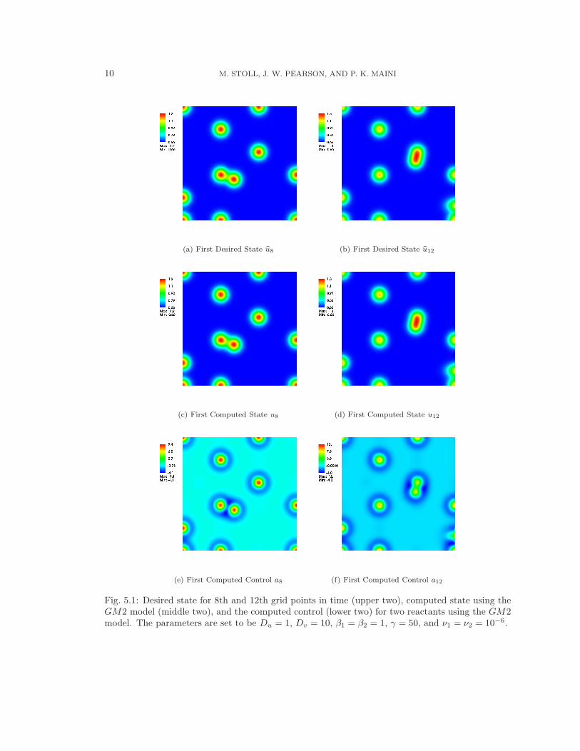
5.1. GM2 model. For both GM2 and GM1 models we start creating desired states usingGaussians placed at different positions in the unit square/cube that might depend on the time t.In Figure 5.1 we illustrate two instances of the desired state and computed results for the GM2formulation, with the parameters set to Du = 1, Dv = 10, β1 = β2 = 1, γ = 50, and ν1 = ν2 = 10−6.

As the regularization parameters become smaller we see that the desired and computed states arevery close. This is reflected in the third set of images within Figure 5.1 where the control is shownwith sometimes rather high values. In Table 5.1 we present iteration numbers for solving this testproblem for a range of degrees of freedom and regularization parameters.

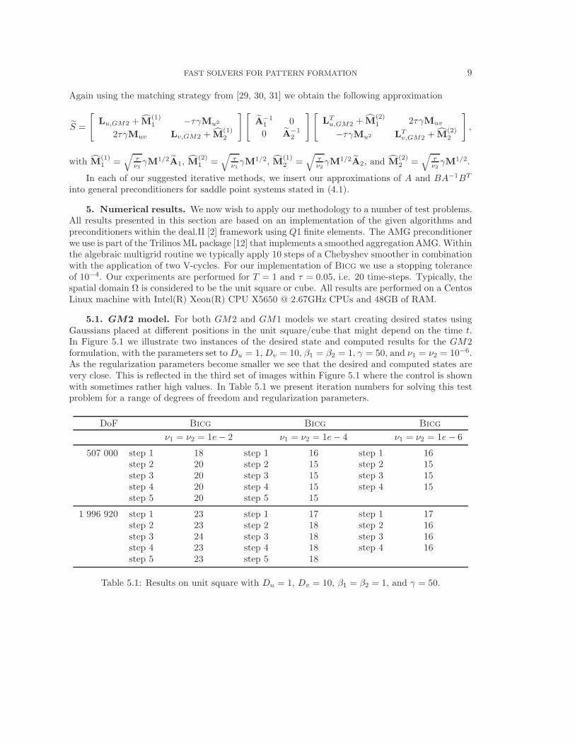
DoF Bicg Bicg Bicg

ν1 = ν2 = 1e− 2 ν1 = ν2 = 1e− 4 ν1 = ν2 = 1e− 6

507 000 step 1 18 step 1 16 step 1 16step 2 20 step 2 15 step 2 15step 3 20 step 3 15 step 3 15step 4 20 step 4 15 step 4 15step 5 20 step 5 15

1 996 920 step 1 23 step 1 17 step 1 17step 2 23 step 2 18 step 2 16step 3 24 step 3 18 step 3 16step 4 23 step 4 18 step 4 16step 5 23 step 5 18

Table 5.1: Results on unit square with Du = 1, Dv = 10, β1 = β2 = 1, and γ = 50.


(a) First Desired State bu8 (b) First Desired State bu12

(c) First Computed State u8 (d) First Computed State u12

(e) First Computed Control a8 (f) First Computed Control a12

Fig. 5.1: Desired state for 8th and 12th grid points in time (upper two), computed state using theGM2 model (middle two), and the computed control (lower two) for two reactants using the GM2model. The parameters are set to be Du = 1, Dv = 10, β1 = β2 = 1, γ = 50, and ν1 = ν2 = 10−6.


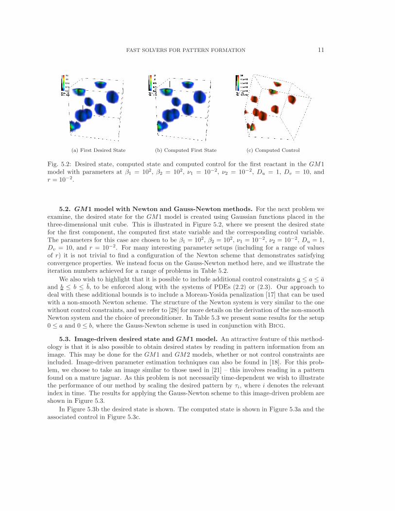
(a) First Desired State (b) Computed First State (c) Computed Control

Fig. 5.2: Desired state, computed state and computed control for the first reactant in the GM1model with parameters at β1 = 102, β2 = 102, ν1 = 10−2, ν2 = 10−2, Du = 1, Dv = 10, andr = 10−2.

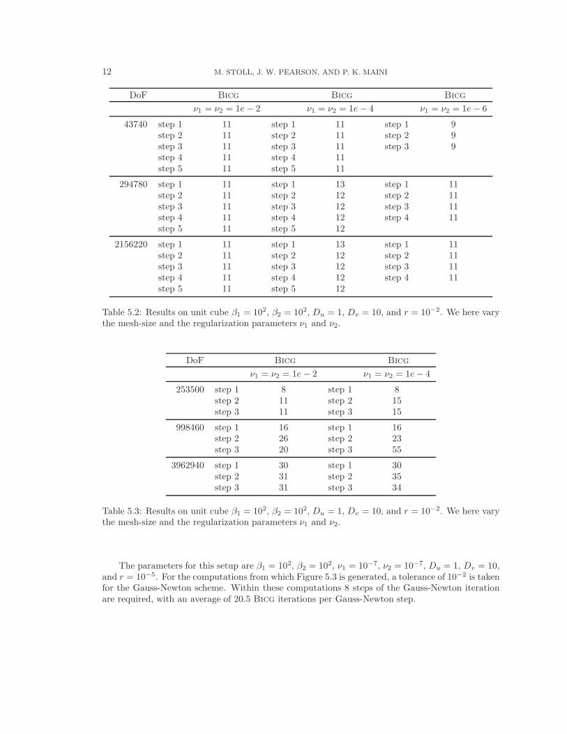
5.2. GM1 model with Newton and Gauss-Newton methods. For the next problem weexamine, the desired state for the GM1 model is created using Gaussian functions placed in thethree-dimensional unit cube. This is illustrated in Figure 5.2, where we present the desired statefor the first component, the computed first state variable and the corresponding control variable.The parameters for this case are chosen to be β1 = 102, β2 = 102, ν1 = 10−2, ν2 = 10−2, Du = 1,Dv = 10, and r = 10−2. For many interesting parameter setups (including for a range of valuesof r) it is not trivial to find a configuration of the Newton scheme that demonstrates satisfyingconvergence properties. We instead focus on the Gauss-Newton method here, and we illustrate theiteration numbers achieved for a range of problems in Table 5.2.

We also wish to highlight that it is possible to include additional control constraints a ≤ a ≤ a

and b ≤ b ≤ b, to be enforced along with the systems of PDEs (2.2) or (2.3). Our approach todeal with these additional bounds is to include a Moreau-Yosida penalization [17] that can be usedwith a non-smooth Newton scheme. The structure of the Newton system is very similar to the onewithout control constraints, and we refer to [28] for more details on the derivation of the non-smoothNewton system and the choice of preconditioner. In Table 5.3 we present some results for the setup0 ≤ a and 0 ≤ b, where the Gauss-Newton scheme is used in conjunction with Bicg.

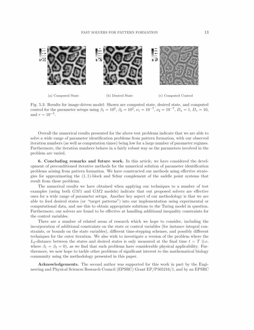
5.3. Image-driven desired state and GM1 model. An attractive feature of this method-ology is that it is also possible to obtain desired states by reading in pattern information from animage. This may be done for the GM1 and GM2 models, whether or not control constraints areincluded. Image-driven parameter estimation techniques can also be found in [18]. For this prob-lem, we choose to take an image similar to those used in [21] – this involves reading in a patternfound on a mature jaguar. As this problem is not necessarily time-dependent we wish to illustratethe performance of our method by scaling the desired pattern by τi, where i denotes the relevantindex in time. The results for applying the Gauss-Newton scheme to this image-driven problem areshown in Figure 5.3.

In Figure 5.3b the desired state is shown. The computed state is shown in Figure 5.3a and theassociated control in Figure 5.3c.


DoF Bicg Bicg Bicg

ν1 = ν2 = 1e− 2 ν1 = ν2 = 1e− 4 ν1 = ν2 = 1e− 6

43740 step 1 11 step 1 11 step 1 9step 2 11 step 2 11 step 2 9step 3 11 step 3 11 step 3 9step 4 11 step 4 11step 5 11 step 5 11

294780 step 1 11 step 1 13 step 1 11step 2 11 step 2 12 step 2 11step 3 11 step 3 12 step 3 11step 4 11 step 4 12 step 4 11step 5 11 step 5 12

2156220 step 1 11 step 1 13 step 1 11step 2 11 step 2 12 step 2 11step 3 11 step 3 12 step 3 11step 4 11 step 4 12 step 4 11step 5 11 step 5 12

Table 5.2: Results on unit cube β1 = 102, β2 = 102, Du = 1, Dv = 10, and r = 10−2. We here varythe mesh-size and the regularization parameters ν1 and ν2.

DoF Bicg Bicg

ν1 = ν2 = 1e− 2 ν1 = ν2 = 1e− 4

253500 step 1 8 step 1 8step 2 11 step 2 15step 3 11 step 3 15



Table 5.3: Results on unit cube β1 = 102, β2 = 102, Du = 1, Dv = 10, and r = 10−2. We here varythe mesh-size and the regularization parameters ν1 and ν2.

The parameters for this setup are β1 = 102, β2 = 102, ν1 = 10−7, ν2 = 10−7, Du = 1, Dv = 10,and r = 10−5. For the computations from which Figure 5.3 is generated, a tolerance of 10−2 is takenfor the Gauss-Newton scheme. Within these computations 8 steps of the Gauss-Newton iterationare required, with an average of 20.5 Bicg iterations per Gauss-Newton step.


(a) Computed State (b) Desired State (c) Computed Control

Fig. 5.3: Results for image-driven model: Shown are computed state, desired state, and computedcontrol for the parameter setups using β1 = 102, β2 = 102, ν1 = 10−7, ν2 = 10−7, Du = 1, Dv = 10,and r = 10−5.

Overall the numerical results presented for the above test problems indicate that we are able tosolve a wide range of parameter identification problems from pattern formation, with our observediteration numbers (as well as computation times) being low for a large number of parameter regimes.Furthermore, the iteration numbers behave in a fairly robust way as the parameters involved in theproblem are varied.

6. Concluding remarks and future work. In this article, we have considered the devel-opment of preconditioned iterative methods for the numerical solution of parameter identificationproblems arising from pattern formation. We have constructed our methods using effective strate-gies for approximating the (1, 1)-block and Schur complement of the saddle point systems thatresult from these problems.

The numerical results we have obtained when applying our techniques to a number of testexamples (using both GM1 and GM2 models) indicate that out proposed solvers are effectiveones for a wide range of parameter setups. Another key aspect of our methodology is that we areable to feed desired states (or “target patterns”) into our implementation using experimental orcomputational data, and use this to obtain appropriate solutions to the Turing model in question.Furthermore, our solvers are found to be effective at handling additional inequality constraints forthe control variables.

There are a number of related areas of research which we hope to consider, including theincorporation of additional constraints on the state or control variables (for instance integral con-straints, or bounds on the state variables), different time-stepping schemes, and possibly differenttechniques for the outer iteration. We also wish to investigate a version of the problem where theL2-distance between the states and desired states is only measured at the final time t = T (i.e.where β1 = β2 = 0), as we find that such problems have considerable physical applicability. Fur-thermore, we now hope to tackle other problems of significant interest to the mathematical biologycommunity using the methodology presented in this paper.

Acknowledgements. The second author was supported for this work in part by the Engi-neering and Physical Sciences Research Council (EPSRC) Grant EP/P505216/1, and by an EPSRC


Doctoral Prize. The authors are grateful for the award of a European Science Foundation (ESF)Exchange Grant under the OPTPDE programme, and express their thanks to the Max PlanckInstitute in Magdeburg.

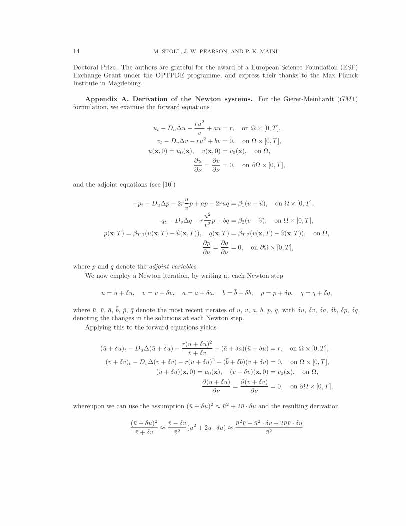
Appendix A. Derivation of the Newton systems. For the Gierer-Meinhardt (GM1)formulation, we examine the forward equations

ut −Du∆u−ru2

v+ au = r, on Ω × [0, T ],

vt −Dv∆v − ru2 + bv = 0, on Ω × [0, T ],

u(x, 0) = u0(x), v(x, 0) = v0(x), on Ω,

∂u

∂ν=∂v

∂ν= 0, on ∂Ω × [0, T ],

and the adjoint equations (see [10])

−pt −Du∆p− 2ru

vp+ ap− 2ruq = β1(u− u), on Ω × [0, T ],

−qt −Dv∆q + ru2

v2p+ bq = β2(v − v), on Ω × [0, T ],

p(x, T ) = βT,1(u(x, T ) − u(x, T )), q(x, T ) = βT,2(v(x, T ) − v(x, T )), on Ω,

∂p

∂ν=∂q

∂ν= 0, on ∂Ω × [0, T ],

where p and q denote the adjoint variables.

We now employ a Newton iteration, by writing at each Newton step

u = u+ δu, v = v + δv, a = a+ δa, b = b+ δb, p = p+ δp, q = q + δq,

where u, v, a, b, p, q denote the most recent iterates of u, v, a, b, p, q, with δu, δv, δa, δb, δp, δqdenoting the changes in the solutions at each Newton step.

Applying this to the forward equations yields

(u+ δu)t −Du∆(u + δu) −r(u + δu)2

v + δv+ (a+ δa)(u + δu) = r, on Ω × [0, T ],

(v + δv)t −Dv∆(v + δv) − r(u + δu)2 + (b+ δb)(v + δv) = 0, on Ω × [0, T ],

(u+ δu)(x, 0) = u0(x), (v + δv)(x, 0) = v0(x), on Ω,

∂(u+ δu)

∂ν=∂(v + δv)

∂ν= 0, on ∂Ω × [0, T ],

whereupon we can use the assumption (u+ δu)2 ≈ u2 + 2u · δu and the resulting derivation

(u+ δu)2

v + δv≈v − δv

v2(u2 + 2u · δu) ≈

u2v − u2 · δv + 2uv · δu

v2


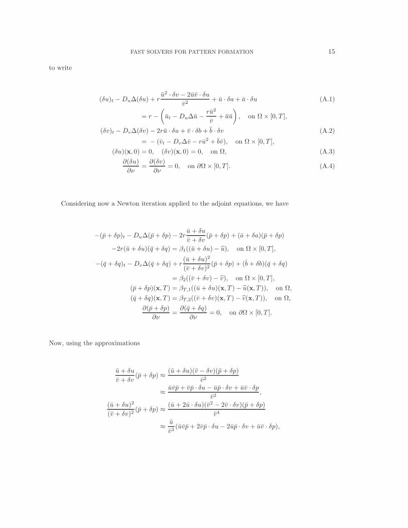
to write

(δu)t −Du∆(δu) + ru2 · δv − 2uv · δu

v2+ u · δa+ a · δu (A.1)

= r −

(ut −Du∆u−

ru2

v+ au

), on Ω × [0, T ],

(δv)t −Dv∆(δv) − 2ru · δu+ v · δb+ b · δv (A.2)

= − (vt −Dv∆v − ru2 + bv), on Ω × [0, T ],

(δu)(x, 0) = 0, (δv)(x, 0) = 0, on Ω, (A.3)

∂(δu)

∂ν=∂(δv)

∂ν= 0, on ∂Ω × [0, T ]. (A.4)

Considering now a Newton iteration applied to the adjoint equations, we have

−(p+ δp)t −Du∆(p+ δp) − 2ru+ δu

v + δv(p+ δp) + (a+ δa)(p+ δp)

−2r(u+ δu)(q + δq) = β1((u + δu) − u), on Ω × [0, T ],

−(q + δq)t −Dv∆(q + δq) + r(u + δu)2

(v + δv)2(p+ δp) + (b+ δb)(q + δq)

= β2((v + δv) − v), on Ω × [0, T ],

(p+ δp)(x, T ) = βT,1((u + δu)(x, T ) − u(x, T )), on Ω,

(q + δq)(x, T ) = βT,2((v + δv)(x, T ) − v(x, T )), on Ω,

∂(p+ δp)

∂ν=∂(q + δq)

∂ν= 0, on ∂Ω × [0, T ].

Now, using the approximations

u+ δu

v + δv(p+ δp) ≈

(u + δu)(v − δv)(p + δp)

v2

≈uvp+ vp · δu− up · δv + uv · δp

v2,

(u+ δu)2

(v + δv)2(p+ δp) ≈

(u + 2u · δu)(v2 − 2v · δv)(p+ δp)

v4

≈u

v3(uvp+ 2vp · δu− 2up · δv + uv · δp),


we may write

− (δp)t −Du∆(δp) − 2rup · δv − vp · δu− uv · δp

v2(A.5)

+ p · δa+ a · δp− 2r(u · δq + q · δu) − β1δu

= β1(u− u) −(−pt −Du∆p− 2r

u

vp+ ap− 2ruq

), on Ω × [0, T ],

− (δq)t −Dv∆(δq) + ru2vp · δu+ uv · δp− 2up · δv

v2+ q · δb+ b · δq − β2δv (A.6)

= β2(v − v) −

(−qt −Dv∆q + r

u2

v2p+ bq

), on Ω × [0, T ],

(δp)(x, T ) = βT,1(δu)(x, T ), (δq)(x, T ) = βT,2(δv)(x, T ), on Ω, (A.7)

∂(δp)

∂ν=∂(δq)

∂ν= 0, on ∂Ω × [0, T ]. (A.8)

Now, the forward and adjoint equations can clearly be derived by differentiating the Lagrangian

JGM1(u, v, a, b, p, q) =β1

2‖u− u‖

2L2(Ω×[0,T ]) +

β2

2‖v − v‖

2L2(Ω×[0,T ])

+βT,1

2‖u(x, T ) − uT ‖

2L2(Ω) +

βT,2

2‖v(x, T ) − vT ‖

2L2(Ω)

+ν1

2‖a‖

2L2(Ω×[0,T ]) +

ν2

2‖b‖

2L2(Ω×[0,T ])

−

∫

Ω×[0,T ]

p

(ut −Du∆u −

ru2

v+ au− r

)

−

∫

Ω×[0,T ]

q(vt −Dv∆v − ru2 + bv

),

with respect to the adjoint variables p, q and the state variables u, v, respectively. Within this costfunctional, we have excluded the constraints on the boundary conditions for readability reasons.To obtain the gradient equations we require for a closed system of equations, we also need todifferentiate the above cost functional with respect to the control variables a and b. Differentiatingwith respect to a gives the requirement

∫

Ω×[0,T ]

(up− ν1a) = 0,

and differentiating with respect to b yields similarly that∫

Ω×[0,T ]

(vq − ν2b) = 0.

Applying a Newton iteration to these equations will give constraints of the form∫

Ω×[0,T ]

(p · δu+ u · δp− ν1δa) = −

∫

Ω×[0,T ]

(up− ν1a), (A.9)

∫

Ω×[0,T ]

(q · δv + v · δq − ν2δb) = −

∫

Ω×[0,T ]

(vq − ν2b), (A.10)


at each Newton step.Therefore the complete system which we will need to solve at each Newton step corresponds

to the adjoint equations (A.5)–(A.8), the gradient equations (A.9) and (A.10), and the forwardequations (A.1)–(A.4).

We now turn our attention to the Schnakenberg (GM2) model, where we wish to deal with theforward equations

ut −Du∆u+ γ(u− u2v) − γa = 0, on Ω × [0, T ],

vt −Dv∆v + γu2v − γb = 0, on Ω × [0, T ],

u(x, 0) = u0(x), v(x, 0) = v0(x), on Ω,

∂u

∂ν=∂v

∂ν= 0, on ∂Ω × [0, T ],

and the adjoint equations (see [10])

−pt −Du∆p+ 2γuv(q − p) + γp = β1(u− u), on Ω × [0, T ],

−qt −Dv∆q + γu2(q − p) = β2(v − v), on Ω × [0, T ],

p(x, T ) = βT,1(u(x, T ) − u(x, T )), q(x, T ) = βT,2(v(x, T ) − v(x, T )), on Ω,

∂p

∂ν=∂q

∂ν= 0, on ∂Ω × [0, T ].

Now, substituting

u = u+ δu, v = v + δv, a = a+ δa, b = b+ δb, p = p+ δp, q = q + δq,

into the forward equations at each Newton step gives

(u+ δu)t −Du∆(u+ δu) + γ((u+ δu) − (u + δu)2(v + δv))

−γ(a+ δa) = 0, on Ω × [0, T ],

(v + δv)t −Dv∆(v + δv) + γ(u+ δu)2(v + δv) − γ(b+ δb) = 0, on Ω × [0, T ],

(u+ δu)(x, 0) = u0(x), (v + δv)(x, 0) = v0(x), on Ω,

∂(u+ δu)

∂ν=∂(v + δv)

∂ν= 0, on ∂Ω × [0, T ],

which we may expand and simplify to give

(δu)t −Du∆(δu) + γ(δu− u2 · δv − 2uv · δu) − γδa (A.11)

= − (ut −Du∆u+ γ(u− u2v) − γa), on Ω × [0, T ],

(δv)t −Dv∆(δv) + γ(u2 · δv + 2uv · δu) − γδb (A.12)

= − (vt −Dv∆v + γu2v − γb), on Ω × [0, T ],

(δu)(x, 0) = 0, (δv)(x, 0) = 0, on Ω, (A.13)

∂(δu)

∂ν=∂(δv)

∂ν= 0, on ∂Ω × [0, T ]. (A.14)


Applying the same substitutions to the adjoint equations gives

−(p+ δp)t −Du∆(p+ δp) + 2γuv((q + δq) − (p+ δp)) + γ(p+ δp)

= β1((u + δu) − u), on Ω × [0, T ],

−(q + δq)t −Dv∆(q + δq) + γu2((q + δq) − (p+ δp))

= β2((v + δv) − v), on Ω × [0, T ],

(p+ δp)(x, T ) = βT,1((u + δu)(x, T ) − u(x, T )), on Ω,

(q + δq)(x, T ) = βT,2((v + δv)(x, T ) − v(x, T )), on Ω,

∂(p+ δp)

∂ν=∂(q + δq)

∂ν= 0, on ∂Ω × [0, T ],

which may then be expanded and simplified to give

− (δp)t −Du∆(δp) + 2γ(vq · δu+ uq · δv + uv · δq (A.15)

− vp · δu− up · δv − uv · δp) + γδp− β1δu

= β1(u− u) − (−pt −Du∆p+ 2γuv(q − p) + γp), on Ω × [0, T ],

− (δq)t −Dv∆(δq) + γ(u2 · δq + 2uq · δu− u2δp− 2up · δu) − β2δv (A.16)

= β2(v − v) − (−qt −Dv∆q + γu2(q − p)), on Ω × [0, T ],

(δp)(x, T ) = βT,1(δu)(x, T ), (δq)(x, T ) = βT,2(δv)(x, T ), on Ω, (A.17)

∂(δp)

∂ν=∂(δq)

∂ν= 0, on ∂Ω × [0, T ]. (A.18)

The forward and adjoint equations can be derived by differentiating the Lagrangian

JGM2(u, v, a, b, p, q) =β1

2‖u− u‖2

L2(Ω×[0,T ]) +β2

2‖v − v‖2

L2(Ω×[0,T ])

+βT,1

2‖u(x, T ) − uT ‖

2L2(Ω) +

βT,2

2‖v(x, T ) − vT ‖

2L2(Ω)

+ν1

2‖a‖

2L2(Ω×[0,T ]) +

ν2

2‖b‖

2L2(Ω×[0,T ])

−

∫

Ω×[0,T ]

p(ut −Du∆u + γ(u− u2v) − γa

)

−

∫

Ω×[0,T ]

q(vt −Dv∆v + γu2v − γb

),

with respect to u, v, p and q, similarly as for the GM1 model. The gradient equations for thisproblem may be derived by differentiating this Lagrangian with respect to the control variables aand b, which gives the conditions

∫

Ω×[0,T ]

(ν1a+ γp) = 0,

∫

Ω×[0,T ]

(ν2b+ γq) = 0.

Applying Newton iteration to these equations gives∫

Ω×[0,T ]

(ν1δa+ γδp) = −

∫

Ω×[0,T ]

(ν1a+ γp), (A.19)

∫

Ω×[0,T ]

(ν2δb+ γδq) = −

∫

Ω×[0,T ]

(ν2b+ γq), (A.20)


at each Newton step.

Hence the system of equations which need to be solved at each Newton step are the adjointequations (A.15)–(A.18), the gradient equations (A.19) and (A.20), and the forward equations(A.11)–(A.14).

REFERENCES

[1] A. Badugu, C. Kraemer, P. Germann, D. Menshykau, and D. Iber, Digit patterning during limb develop-

ment as a result of the BMP-receptor interaction, Sci. Rep., 991 (2012), pp. 1–13.[2] W. Bangerth, R. Hartmann, and G. Kanschat, deal.II—a general-purpose object-oriented finite element

library, ACM Trans. Math. Software, 33 (2007), pp. Art. 24, 27.[3] M. Benzi, G. H. Golub, and J. Liesen, Numerical solution of saddle point problems, Acta Numer, 14 (2005),

pp. 1–137.[4] M. Benzi, E. Haber, and L. Taralli, A preconditioning technique for a class of PDE-constrained optimization

problems, Adv. Comput. Math., 35 (2011), pp. 149–173.[5] V. Castets, E. Dulos, J. Boissonade, and P. De Kepper, Experimental evidence of a sustained standing

Turing-type nonequilibrium chemical pattern, Phys. Rev. Lett., 64 (1990), pp. 2953–2956.[6] I. S. Duff, A. M. Erisman, and J. K. Reid, Direct methods for sparse matrices, Monographs on Numerical

Analysis, The Clarendon Press Oxford University Press, New York, 1989.[7] A. D. Economou, A. Ohazama, T. Porntaveetus, P. T. Sharpe, S. Kondo, M. A. Basson, A. Gritli-

Linde, M. T. Coburne, and J. B. A. Green, Periodic stripe formation by a Turing mechanism operating

at growth zones in the mammalian palate, Nat. Genet., 44 (2012), pp. 348–351.[8] H. C. Elman, D. J. Silvester, and A. J. Wathen, Finite elements and fast iterative solvers: with applications

in incompressible fluid dynamics, Numerical Mathematics and Scientific Computation, Oxford UniversityPress, New York, 2005.

[9] R. Fletcher, Conjugate gradient methods for indefinite systems, in Numerical Analysis (Proc. 6th BiennialDundee Conf., Univ. Dundee, Dundee, 1975), Springer, Berlin, 1976, pp. 73–89. Lecture Notes in Math.,Vol. 506.

[10] M. R. Garvie, P. K. Maini, and C. Trenchea, An efficient and robust numerical algorithm for estimating

parameters in Turing systems, J. Comput. Phys., 229 (2010), pp. 7058–7071.[11] M. R. Garvie and C. Trenchea, Identification of space-time distributed parameters in the Gierer-Meinhardt

reaction-diffusion system, SIAM J. Appl. Math., 74–1 (2014), pp. 147–166.[12] M.W. Gee, C.M. Siefert, J.J. Hu, R.S. Tuminaro, and M.G. Sala, ML 5.0 smoothed aggregation user’s

guide, Tech. Report SAND2006-2649, Sandia National Laboratories, 2006.[13] A. Gierer and H. Meinhardt, A theory of biological pattern formation, Biol. Cybernet., 12 (1972), pp. 30–39.[14] G. H. Golub and C. F. Van Loan, Matrix computations, Johns Hopkins Studies in the Mathematical Sciences,

Johns Hopkins University Press, Baltimore, MD, third ed., 1996.[15] E. Haber, U. M. Ascher, and D. Oldenburg, On optimization techniques for solving nonlinear inverse

problems, Inverse Probl., 16 (2000), pp. 1263–1280.[16] M. R. Hestenes and E. Stiefel, Methods of conjugate gradients for solving linear systems, J. Res. Nat. Bur.

Stand., 49 (1952), pp. 409–436 (1953).[17] M. Hinze, R. Pinnau, M. Ulbrich, and S. Ulbrich, Optimization with PDE constraints, Mathematical

Modelling: Theory and Applications, Springer-Verlag, New York, 2009.[18] C. Hogea, C. Davatzikos, and G. Biros, An image-driven parameter estimation problem for a reaction–

diffusion glioma growth model with mass effects, J. Math. Biol., 56 (2008), pp. 793–825.[19] K. Ito and K. Kunisch, Lagrange multiplier approach to variational problems and applications, vol. 15 of

Advances in Design and Control, Society for Industrial and Applied Mathematics (SIAM), Philadelphia,PA, 2008.

[20] Y. A. Kuznetsov, Efficient iterative solvers for elliptic finite element problems on nonmatching grids, Russ.J. Numer. Anal. M., 10 (1995), pp. 187–211.

[21] R. T. Liu, S. S. Liaw, and P. K. Maini, Two-stage Turing model for generating pigment patterns on the

leopard and the jaguar, Phys. Rev. E, 74 (2006), pp. 011914–1.[22] M. F. Murphy, G. H. Golub, and A. J. Wathen, A note on preconditioning for indefinite linear systems,

SIAM J. Sci. Comput, 21 (2000), pp. 1969–1972.[23] J. D. Murray, Mathematical biology. Vol. 2: Spatial models and biomedical applications. 3rd revised ed., New

York, NY: Springer, 2003.


[24] J. Nocedal and S. J. Wright, Numerical optimization, Springer Series in Operations Research, Springer-Verlag, New York, 1999.

[25] , Numerical optimization, Springer Series in Operations Research and Financial Engineering, Springer,New York, second ed., 2006.

[26] Q. Ouyang and H. L. Swinney, Transition from a uniform state to hexagonal and striped Turing patterns,Nature, 352 (1991), pp. 610–612.

[27] C. C. Paige and M. A. Saunders, Solutions of sparse indefinite systems of linear equations, SIAM J. Numer.Anal., 12 (1975), pp. 617–629.

[28] J. W. Pearson and M. Stoll, Fast iterative solution of reaction-diffusion control problems arising from

chemical processes, SIAM J. Sci. Comp, 35 (2013), pp. B987–B1009.[29] J. W. Pearson, M. Stoll, and A. J. Wathen, Regularization-robust preconditioners for time-dependent

PDE-constrained optimization problems, SIAM J. Matrix Anal. Appl., 33 (2012), pp. 1126–1152.[30] J. W. Pearson and A. J. Wathen, A new approximation of the Schur complement in preconditioners for

PDE-constrained optimization, Numer. Linear Algebra Appl., 19 (2012), pp. 816–829.[31] , Fast iterative solvers for convection-diffusion control problems, Electron. Trans. Numer. Anal., 40

(2013), pp. 294–310.[32] Y. Saad, Iterative methods for sparse linear systems, Society for Industrial and Applied Mathematics, Philadel-

phia, PA, 2003.[33] J. Schnakenberg, Simple chemical reaction systems with limit cycle behaviour, J. Theoret. Biol., 81 (1979),

pp. 389–400.[34] R. Sheth, L. Marcon, M. F. Bastida, M. Junco, L. Quintana, R. Dahn, M. Kmita, J. Sharpe, and

M. A. Ros, Hox genes regulate digit patterning by controlling the wavelength of a Turing-type mechanism,Science, 338 (2012), pp. 1476–1480.

[35] F. Troltzsch, Optimal control of partial differential equations: theory, methods and applications, AmericanMathematical Society, 2010.

[36] A. Turing, The chemical basis of morphogenesis, Philos. Trans. R. Soc. London, Ser. B, 237 (1952), pp. 37–72.[37] A. J. Wathen and T. Rees, Chebyshev semi-iteration in preconditioning for problems including the mass

matrix, Electron. Trans. Numer. Anal., 34 (2008), pp. 125–135.

Documents

FAST SOLVERS FOR OPTIMAL CONTROL … SOLVERS FOR OPTIMAL CONTROL PROBLEMS FROM PATTERN FORMATION MARTIN STOLL∗, JOHN W. PEARSON†, AND PHILIP K. MAINI‡ Abstract. The modelling