Fast Volume Render ingand Deformation Algor ithms

A Disser tation

Submitted to the Faculty of Mathematics and Computer Science

of the University of Mannheim

for the Degree of Doktor der Naturwissenschaften (Dr. rer . nat.)

By

Master of Science Haixin Chen

from Hunan

P.R. China

Mannheim, 2001

1

Chapter 1

Introduction

Seeing is believing. Seeing plays the most important role for a human being to get

information from the real world.

Today we can see the world not only with our eyes. With new instruments and

techniques we can also observe the things that could not be seen with our naked eyes before.

Thus the view of a human being is widely expanded, both macroscopically and

microcosmically.

Such magic instruments include among others the advanced imaging equipment used in

medical fields—computer tomography (CT) and magnet resonance tomography (MRI). Since

the first CT imaging equipment was invented and applied in medicine in the 1970s,

tomography techniques had brought the physicians brand-new approaches to diagnose

suspicious diseases and plan high-risk operations.

Different from the traditional X-ray images, each slice of the tomography images is

marked with its relative position in the 3D space. Hence, using tomopraphy image sequences,

experienced physicians can imagine the 3D structures of the observed objects. In this way

physicians can more precisely diagnose and make more optimal operation plans to minimize

potential risks for diagnostics and therapy.

2

The problem is, however, not every physician is experienced. Even a well trained

physician may lack enough insight to imagine the 3D structures of a patient’s organ from a

sequence of CT images. Is there an easy method to reveal the information embedded in the

tomography images? Fortunately such a method has been proposed for a long time, it is called

volume rendering—the theme of my dissertation.

1.1 Motivations Volume rendering originated from the medical applications, but it has been widely used

in other engineering and research fields. In such fields, volume rendering is used as a tool to

reveal the embedded key information in the data sets or generate vivid visual demonstrations.

An example is the geological research, in which acoustic waves generated by an artificial

explosive are sampled and used to produce 3D maps of geological structures below the

surface of the earth. Another typical example is the simulation based on computational fluid

dynamics which produces data on a 3D grid that is used to analyze the aerodynamic property

of a designed automobile or predict the regional weather. The 3D data for volume rendering

can also be artificially produced through a process called voxelization from existing 3D

surface models or data sampled by 3D laser-scanners.

In most of the applications, the 3D data to be processed is of very huge size. Volumes

having many megabytes of data are quite normal. The huge size of volume data makes

volume rendering extremely computationally expensive. Rendering a volume data for

interactive applications like operation planning usually requires large amounts of processing

power and high memory bandwidth. In the last decade, different methods have been proposed

to achieve interactivity in volume rendering. Common approaches are using algorithmic

optimizations [1], taking advantage of the super computing power of expensive massive

parallel computers [2] or utilizing special-purposed hardware [3, 4, 5].

Currently, real time volume rendering can be achieved only by using special-purpose

hardware or parallel computer systems. Despite the rapid increase of the commonly available

computing power and memory bandwidth, which enables the interactive (>1 frame per

second) volume rendering of middle sized volume data sets with software-only systems like

VolPack [6] and VGL [7] on state-of-the-art desktop PCs, a considerable performance gap

does exist between the software-only volume rendering systems and the volume rendering

systems which use special-purpose hardware or massive parallel computer systems. On the

other hand, the available volume resolution keeps increasing. For example, the most advanced

tomography imaging systems can now deliver volumes with 10243 voxels. Using the pure

3

software system, it is impossible to achieve interactivity for such huge volume data, since the

required memory bandwidth for rendering such data sets in real time alone presents an

unsolvable bottleneck for the general-purposed PCs. As the massive parallel computing is not

widely available for most users, the best way to achieve real time volume rendering is using

dedicatedly designed volume graphics hardware.

VolumePro [5] is currently the fastest PCI-based commercial special-purposed hardware

for volume rendering. It integrates 8 rendering pipelines on a single chip and can deliver 30

fps rendering speed for 2563 data sets. However, it does not support perspective projection

which is essential for many applications.

Recently Vettermann et al. [8] proposed the VGE architecture. VGE supports the

algorithmic optimizations like early-ray-termination and space-leaping. The data hazard

caused by algorithmic optimization is hidden by a multi-threading rendering scheme, thus the

rendering pipeline can run at full speed. The simulation results show that the VGE

architecture can achieve a similar performance as VolumePro with only one single rendering

pipeline when most of the voxels are mapped either transparent or opaque. Unlike

VolumePro, VGE is based on ray casting algorithms and supports both parallel and

perspective projection. One problem with VGE is that the achieved frame rate depends on the

opacity transfer functions. There is a performance decrease of a factor of two or even more

when the volume is semi-transparently mapped, compared to the transparent-opaque mapped

case. This is because in the current implementation, early-ray-termination and space-leaping

can only save the operations for the occluded voxels and empty voxels separately. No

measures are taken to reduce the calculation in the semi-transparent regions.

In order to avoid the performance decrease of VGE in rendering semi-transparently

mapped volume object, we aim to develop algorithms to improve the rendering speed for the

semi-transparently mapped volume. We solve this problem by exploiting the spatial

coherence in volume data. In this way we achieve the required performance gain which

guarantees that VGE can render volume objects in real time under arbitrarily selected opacity

transfer functions.

The spatial coherence in the volume data need to be encoded in a preprocessing stage.

The primitive approach for encoding the spatial coherence consumes several minutes to hours

for middle-sized volume data sets. Therefore it is unusable in real applications. In order to

solve this problem, we investigate different approaches to reduce the preprocessing time and

develop a Taylor-expansion based spatial coherence encoding method. The new encoding

4

method requires less than 12 seconds for data sets with about 8 million voxels, thus it allows

the new volume rendering acceleration technique to be integrated in real applications.

Another objective of this research work is to develop fast volume deformation methods.

The simulation of volumetric object deformation is a key technique for virtual reality

applications like medical training systems. Volume rendering of deformable objects can be

implemented either by directly using a sequence of dynamical volume data, or by using a

single static volume data which is resampled according to the deformation rules to produce

the deformation effects. The former approach has several drawbacks. First, even the most

advanced imaging instruments have a limited sampling rate. When the deforming object is

imaged dynamically, the resulting volume data suffers from motion blur. Correcting the

motion blur is difficult and time-consuming due to the large number of voxel slices. Second, a

volume sequence requires much more storage space than a single volume data set. Loading

the volume sequences into memory in real time alone presents a bottleneck of memory

bandwidth. Moreover, such a deformation procedure is not flexible, since the deformation is

fixed. However, in applications like surgical simulation, the deformation of a volume object

should be determined by interactive user input. By using the latter approach we can avoid the

above mentioned drawbacks. Hence, the volume deformation is usually simulated by

resampling an original volume data, guided by the underlying deformation rules.

The brute force deformation method generates an intermediate deformed volume by

resampling the original volume before the deformed volume is rendered. Hereby the volume

deformation simulation consists of two separate processes: volume deformation and volume

rendering of the deformed volume. Nevertheless, the volume is an exhaustive enumeration

representation of objects. It is prohibitively computationally expensive to deform a volume

object by deforming each primitive of the volume object due to the huge amount of primitives

(voxels). The separation of the rendering process from the deformation process requires the

whole volume to be deformed before it is rendered. This leads to considerable waste of

computational resources, since usually only a limited portion of the volume has a contribution

to the final image.

Recognizing the drawback of separating the deformation process from the rendering

process, we unify these two processes in our fast volume deformation method by using

inverse-ray-deformation. In the unified deforming/rendering process, the ray is cast along the

trajectory which is deformed opposite to the expected deformation. The computational

complexity is therefore reduced to the half, since the intermediate step to reconstruct a

5

deformed volume is saved. Additionally, the performance can be further increased by

incorporating existing algorithmic optimization techniques into the deformation process.

1.2 Contributions of This Work The contributions of this dissertation include the following aspects:

• A new ray casting acceleration method. The acceleration approach speeds up the

rendering of semi-transparently mapped volume by a factor of two or more by

exploiting the spatial coherence in volume data sets. Thus it enables VGE to render

volume objects in real time under arbitrarily selected opacity transfer functions.

• An efficient preprocessing algorithm for encoding the spatial coherence in volume

data sets. Compared to the primitive approach which consumes several minutes to

several hours for encoding volumes with about 8 million voxels, the proposed

preprocessing algorithm needs less than 12 seconds for the same data sets. Hence,

it makes the new ray casting acceleration method applicable in real applications.

• We combine a B-spline presentation free-form-deformation with the inverse-ray-

deformation. Such a combination has the following benefits in the simulation of

volume deformation:

a) The calculation and the memory space for generating and storing an

intermediate deformed volume are not required any more.

b) Volume objects can be deformed into arbitrary form.

• Methods to adjust shading and opacity in the deformed space. In order to correctly

calculate the shading and the attenuation of ray intensities, one needs to know the

deformation function at any sample point (and the Jacobian of the deformation

function). The B-spline presentation free-form-deformation is given in a recursive

form and cannot be used directly for the shading and opacity adjustment. This

dissertation proposes an efficient method for the estimation of the local

deformation function.

• An approach for rendering deformed volume objects and undeformed objects in

the same scene.

• An adaptive ray division algorithm. During ray casting in the deformed space, the

ray trajectories are approximated by polylines. The length of the polylines are

determined by considering the local curvature along the deformed rays. In this

way, relative longer polylines are automatically selected in the slightly deformed

6

regions, and fine polylines are used in the heavily deformed regions. Thus it

reduces the deformation calculation in the slightly deformed region without loss of

the spatial continuity of the simulated deformation .

• A speedup factor of 2.34~6.56 in rendering heavily deformed volume objects by

combining early-ray-termination, space-leaping and spatial coherence acceleration

in the new deformation algorithm.

1.3 Outline of This Dissertation The thesis consists of two parts.

Chapters 2-4 belong to the first part. In this part chapter 2 presents the background of

volume rendering. Chapter 3 discusses the existing algorithms for volume rendering and the

commonly used volume rendering acceleration techniques. In chapter 4 we develop the new

spatial coherence acceleration algorithms. We apply the new spatial coherence acceleration

technique to both the shear-warp algorithm and the ray casting algorithm. The former

implementation of spatial coherence acceleration techniques encodes spatial coherence in data

structures like octrees and pyramids. Using such data structures is not efficient due to the

overhead of traversing spatial data structures which requires analytic geometry calculations,

e.g. intersecting rays with axis-aligned boxes. We avoid the overhead by saving the spatial

coherence information with each voxel in form of the coherence distance. The coherence

distance can therefore be retrieved by the same addressing arithmetic for voxel addressing,

making the acceleration fully available in the rendering phase. The coherence acceleration

techniques need to encode the spatial coherence information in a preprocessing stage. The

brute force encoding method consumes tens of minutes to several hours to encode the

coherence distance. I invented an efficient Taylor expansion based encoding method which

reduces the preprocessing time to less than 12 seconds for data sets with 8M voxels.

The second part of the thesis addresses the volume deformation algorithms. It includes

chapter 5-6. Chapter 5 is about the basis of object deformation. In chapter 6 we discuss the

new volume deformation methods. The new volume deformation method combines inverse-

ray-deformation with the uniform B-spline representation of the free-form-deformation. We

study how to approximate the deformed ray trajectory with polyline segments. Unlike the

previous method which simply divides the ray into equal-distant segments, our method

divides the ray by considering the local deformation amplitude. In this way the spatial

continuity of the deformation is guaranteed. Another work is for opacity compensation. After

the deformation, the density distribution within the volume is changed, therefore the opacity

7

value of the sample points should be corrected to reflect the change of volume density. Till

now no previous work has addressed this problem. An opacity compensation scheme by

considering the local volume change is developed in this chapter. We also develop the

shading adjustment method in this chapter. The shading adjustment involves the inverse

transformation of the estimated normal vector in the original volume. By exploiting the

continuous property of the B-spline FFD (We use degree 3 B-Spline functions. The

deformation continuity is therefore C1), we develop the method to estimate the local

deformation function as well as the normal transformation matrix required by the shading

adjustment. We incorporate the existing ray casting acceleration techniques into the new

deformation procedure. In the end of chapter 6 we present the experimental results and

discuss the factors that affect the performance of the ray casting acceleration techniques.

Chapter 7 summarizes the work done and indicates the future work.

8

ii

Dekan: Professor Dr . Herber t Popp, Universität Mannheim

Referent: Pr iv.-Doz. Dr . Jürgen Hesser , Universität Mannheim

Korreferent: Professor Dr . Chr istian Schnörr , Universität Mannheim

Tag der mündlichen Prüfung: 28. November 2001

iii

Abstract

Volume data provides a unified description for the surface and inner structures of solidobjects. Volume visualization is therefore attractive for applications like surgical operationsimulation. The huge number of volume primitives (voxels) in a volume of reasonable size,however, leads to high computational expense. Interactive rendering and deformation of thevolumetric object with brute force algorithms cannot be achieved on state of the artcomputing systems.

In this dissertation I developed two new algorithms for the acceleration of direct volumerendering and volume deformation.

The first algorithm accelerates the ray casting process. It is commonly observed that theray casting acceleration techniques like space-leaping and early-ray-termination are onlyefficient when most of the voxels in a volume are mapped either opaque or transparent. Whenmany voxels are mapped semi-transparent, the frame rate of rendering will decrease. Our goalis to improve the performance of ray casting of semi-transparently mapped volumes by afactor of 2~3 times, so that the hardware pipeline [8] can render middle sized volumes witharbitrary opacity transfer functions in real time. Our new algorithm achieved this by reducingthe computational cost in semi-transparent regions by exploiting the opacity coherence inobject space. This is realized with the help of pre-computed coherence distances. Therendering speed for semi-transparently mapped volumes is increased by a factor between 1.90and 3.49. We developed an efficient algorithm to encode the coherence information, whichrequires less than 12 seconds for data sets with about 8 million voxels.

The second algorithm is for volume deformation. Unlike the traditional method, ourmethod incorporates the two stages of volume deformation, i.e. volume deforming andvolume rendering, into a single process. This is implemented by combining the free-form-deformation and inverse-ray-deformation in our approach. Instead of deforming each voxel togenerate an intermediate deformed volume, the algorithm directly follows the inverselydeformed ray to generate the deformation, thus it saves the involved computations toreconstruct the intermediate deformed volume and memory resource for storing the deformedvolume. The smoothness of the deformation is guaranteed by adaptive ray division whichmatches the amplitude of local deformation. Unlike the previous implementation, our shadingcalculation in the deformed space is still gradient-based. This is done by backwardtransforming of the normal vector. We have shown that there is no problem of merging theray casting acceleration techniques with the new deformation process, thus we achieve anadditional speedup of factor 2.34~6.58 to the new deformation process.

Key Words: Volume Rendering, Volume Deformation, Algorithm Optimization, RayCasting, Inverse Ray Deformation, Free Form Deformation.

iv

“Seeing is believing!”

v

Acknowledgements

This work is supported by the DAAD (Deutscher Akademischer Austauchdienst). I would like

to thank DAAD and many of its employees, especially Mrs. Schädlich, who provided me their

generous help whenever possible.

My thanks go also to the CEM(Chinese Education Ministry) who provided me the chance

to finish my doctor research in Germany and I treasure very much the chance that enables me

to learn many things from one of the best cultures in the world.

I am very thankful for many people who contributed to this work and provided their

supports throughout my work on this thesis. First of all, I would like to thank my advisor,

Prof. Dr. Männer, who provided me a very good working environment and supported my

work whenever he could. I would also like to thank Dr. Hesser. My whole work was done

under his guidance. He helped me overcome my language problem and made the research full

of fun. I benefited indeed much from our lively discussions, from his good ideas and

suggestions.

I also want to express my sincere thanks to Ulrike Höfer and Klaus Kornmesser for

providing me a stable computing environment by being always on call to fix system problems.

From them I also learned many German cultures and customs. I did enjoy the cooperation

with them.

Special thanks go to Bernd Vettermann who offered me his experimental source codes

for volume rendering. Although I developed a new ray caster all by myself, I did borrow

something from his program.

vi

I thank also Dennis Maier, a perfect Sino-German bilinguist, for many helps he offered

to my research.

I thank Ulrich Müller for the proofreading of my dissertation.

Special regards to Karsten Mühlman, Marc Deutscher, Andreas Wurz, Joachim Gläß,

Gerhard Lienhart, Andreas Kugel, Peter Dillinger, Markus Schill, Clemens Wagner, Eckart

Bindewald, Andrea Seeger, and Christiane Glasbrenner for the conveniences they provided

me.

Sincere thanks go to also professor Shen Zhenkang and many others who helped me

during this period of time but are not listed here.

I thank my grandmother and my parents who steadily supported my study overseas.

My wife made the greatest supports for my work during this period of time, I dedicate

this thesis to my wife.

vii

Contents

Acknowledgements..................................................................................................................

1 Introduction .........................................................................................................................1

1.1 Motivations.......................................................................................................................2

1.2 Contributions of This Work ............................................................................................5

1.3 Outline of This Dissertation.............................................................................................6

2 Background of Volume Graphics........................................................................................9

2.1 Volume Data.....................................................................................................................9

2.2 Typical Volume Visualization Process .........................................................................13

2.3 Surface Based Volume Rendering ...............................................................................15

2.3.1 Traditional 3D Graphics ......................................................................................15

2.3.2 Extract Surface Model from Volume Data .......................................................17

2.3.3 Discussion on Surface-Based Volume Rendering .........................................18

2.4 Volume Rendering Equation .........................................................................................20

2.5 Volume Resampling.......................................................................................................26

2.5.1 Nearest Neighbor Interpolation............................................................................27

viii

2.5.2 Linear Interpolation .............................................................................................27

2.5.3 High Order Interpolation......................................................................................28

2.6 Shading Estimation for Volume Rendering...................................................................30

2.6.1 Phong Shading Model ........................................................................................31

2.6.2 Gradient Estimation.............................................................................................33

2.6.3 Shading Calculation............................................................................................352.7 Chapter Summary...........................................................................................................35

3 Volume Render ing Algor ithms..........................................................................................37

3.1 Existing Volume Rendering Algorithms........................................................................38

3.1.1 The Splatting Algorithm.......................................................................................38

3.1.2 3D Texture Mapping............................................................................................39

3.1.3 Ray Casting Algorithms.......................................................................................42

3.1.4 Hybrid Algorithms...............................................................................................45

3.2 Volume Rendering Accelerating Techniques.................................................................48

3.2.1 Coherency Acceleration.......................................................................................49

3.2.2 Presentation Acceleration.....................................................................................50

3.2.3 Early-ray-termination...........................................................................................52

3.2.4 Preprocessing.......................................................................................................53

3.3 Chapter Summary...........................................................................................................54

4 Algor ithms For Exploiting Coherence in Volume Data..................................................57

4.1 Introduction....................................................................................................................57

4.2 Accelerating the Shear-Warp Algorithm with Scanline Coherence Encoding..............60

4.2.1 Implementation of Earlier Shear-Warp Algorithms.............................................60

4.2.2 Encoding all three Coherence Forms in the Voxel Scanline..............................63

4.2.3 Implementation of the New Shear-Warp Algorithm............................................66

4.2.4 Results..................................................................................................................70

4.2.5 Discussions...........................................................................................................76

4.3 Accelerating the Ray Casting.........................................................................................77

4.3.1 Motivation............................................................................................................77

4.3.2 Theoretical Bases of Coherence Encoding-based Acceleration...........................78

4.4 Spatial Coherence Encoding..........................................................................................82

4.4.1 Introduction..........................................................................................................82

4.4.2 The Brute Force EDC...........................................................................................85

ix

4.4.3 The Taylor-Expansion-based EDC......................................................................90

4.5 Implementation of the Accelerated Ray-casting Algorithm...........................................98

4.6 Results and Analyses....................................................................................................102

4.7 Discussions...................................................................................................................111

4.8 Chapter Summary.........................................................................................................115

5 Object Deformation Techniques.....................................................................................117

5.1 Geometric deformation methods..................................................................................118

5.2 Physically-based Object Deformation..........................................................................122

5.3 Early Work for Deformation Simulation of Volumetric Objects.................................127

5.4 Chapter Summary.........................................................................................................128

6 Ray-Casting in the Deformed Space................................................................................131

6.1 Ray-Casting Deformable Objects by Inverse-Ray-Deforming....................................132

6.2 Ray-Casting in the Deformed Space............................................................................134

6.2.1 Implementing FFD with a Uniform B-spline Grid.............................................134

6.2.2 The Inverse-Deformed Ray Trajectory in the Deformed Space.......................138

6.2.3 Local Curvature Estimation...............................................................................140

6.2.4 Volume Compositing in the Deformed Space...................................................142

6.3 Shading in the Deformed Space...................................................................................146

6.4 Rendering Deformable and Undeformable Objects in the Same Scene.......................149

6.5 Algorithmic Optimizations...........................................................................................151

6.6 Experimental Results and Analyses.............................................................................151

6.7 Conclusions..................................................................................................................163

7 Conclusions........................................................................................................................165

7.1 Final Summary.............................................................................................................165

7.2 Future Directions..........................................................................................................169

Appendix A: Render ing Results..........................................................................................171

Appendix B: The Volume Ray Casting and Deformation Program................................177

Bibliography..........................................................................................................................191

x

List of Tables

Table 4.1 Performance comparison between the new algorithm and VolPack.........................70

Table 4.2 The performance of the spatial coherence accelerated ray casting by using the

brute force EDC.......................................................................................................104

Table 4.3 The performance of the spatial coherence accelerated ray casting by using the

Taylor expansion based EDC...................................................................................104

Table 4.4 The experimental results for volume data whose voxels are mapped either

empty or opaque.....................................................................................................105

Table 6.1 Comparison of rendering times between two shading schemes.............................155

Table 6.2 Comparison of rendering times between the optimized algorithm and the brute

force algorithm.........................................................................................................155

Table 6.3 Ratios of overall sample number between the non-optimized deformation

algorithm and the optimized deformation algorithm.................................................159

Table 6.4 The deformation times for different brick sizes......................................................163

xi

List of Figures

2.1 The drawback of polygon-mesh based surface models.......................................................10

2.2 Scene of voxelized geometric models in flight simulation.................................................11

2.3 Grid types of volume objects..............................................................................................12

2.4 Irregular grid caused by volume deformation.....................................................................12

2.5 The typical volume visualization process...........................................................................13

2.6 Preprocessing of volume data.............................................................................................14

2.7 Pipeline archicture of OpenGL...........................................................................................17

2.8 Images rendered by the surface-based volume rendering...................................................19

2.9 Ray-voxel interaction..........................................................................................................21

2.10 A ray penetrating the volume............................................................................................24

2.11 Discretizing the ray trajectory in the volume....................................................................24

2.12 The nearest neighbor interpolation function.....................................................................27

2.13 The linear interpolation function.......................................................................................28

2.14 Diffuse reflection model...................................................................................................31

2.15 Specular reflection for Phong shading model...................................................................32

3.1 Volume Rendering by Splatting..........................................................................................38

xii

3.2 Slices through the volume data in the parallel projection...................................................40

3.3 Concentric spheres for a perspective projection in 3D texture mapping............................41

3.4 Ray casting (parallel projection).........................................................................................43

3.5 The digital differential analyzer (DDA) for volume navigation.........................................44

3.6 The 6-connected path Bresenham algorithm for volume navigation..................................44

3.7 Shear-warp transformation..................................................................................................47

3.8 The performance benchmarks of different processors from AMD and Intel......................48

3.9 Ray-casting of hierarchical enumeration............................................................................51

3.10 Distance coding.................................................................................................................52

4.1 Coherence in volume data...................................................................................................58

4.2 Three data structures of the run-length encoded volume....................................................61

4.3 Offsets of pixels in a scanline of the intermediate image...................................................62

4.4 Traversal of voxel and image scanlines..............................................................................63

4.5 Linearization of the opacity curve along a voxel scanline.................................................64

4.6 Pseudo-code for encoding homogeneity and linearity in a voxel scanline.........................65

4.7 Pseudo-code for the new shear-warp algorithm............................................................67-69

4.8 Image quality comparison between the new shear-warp algorithm and VolPack..............71

4.9 Image quality comparison between the new shear-warp algorithm and the 3D

texture mapping technique....................................................................................................72

4.10 The influence of encoding error........................................................................................73

4.11 The influence of encoding error on the performance of the new algorithm.....................74

4.12 The rendering of a voxel scanline.....................................................................................75

4.13 Approximating the voxel opacity value curve with piecewise linear segments...............79

4.14 Shading calculation in the coherent region.......................................................................80

4.15 The tri-linear interpolation for continuous line drawing based ray-casting......................81

4.16 Exploiting coherence in ray casting..................................................................................82

4.17 Arbitrary voxel traversal order for ray-casting.................................................................83

4.18 Coherence encoding for ray casting..................................................................................84

4.19 Space-leaping for ray casting using the encoded distance in a distance array..................85

4.20 Determining possible ray directions in 3D space..............................................................86

4.21 Determining the initial coherence distance.......................................................................87

4.22 The pseudo codes for the brute force EDC algorithm.................................................88-89

4.23 Drawback of examining less viewing directions (2D case)..............................................90

4.24 The selected ray directions for different candidate coherence distance............................91

xiii

4.25 The pseudo codes for the Taylor expansion based EDC algorithm..................................96

4.26 Pyramid hierarchical data structure in 1D case.................................................................97

4.27 The kernel pseudo code of the new ray casting algorithm........................................99-100

4.28 The main window of our ray casting program................................................................101

4.29 The dialog pad for interactive control of visualization parameters.................................102

4.30 Rendition of volumes different opacity transfer functions......................................106-107

4.31 The impact of noise on the performance. .......................................................................108

4.32 The effect of filtering the noise in volume data..............................................................108

4.33 The impact of the encoding error to the performance of the new algorithm..................109

4.34 Influence of light distance to the image quality..............................................................110

4.35 Shading comparison between the new algorithm and VolPack......................................111

4.36 Two strategies for opacity curve approximation.............................................................114

5.1 Global twist deformation..................................................................................................119

5.2 Free-form-deformation......................................................................................................120

5.3 Finite element representation of object.............................................................................124

5.4 Mass-spring representation of deformable object.............................................................125

5.5 Lennard-Jones type function.............................................................................................126

6.1 Inversely deforming rays to generate visual effects of deformation.................................132

6.2 Ray deflector.....................................................................................................................134

6.3 A comparison between B-spline curve and Bézier curve.................................................135

6.4 Determining ray trajectory in the deformed space............................................................138

6.5 The relation between the polyline length and the local curvature radius..........................140

6.6 The pseudo code for ray casting in deformed space..................................................143-144

6.7 Mismatch of deformed ray segments to the standard sample unit....................................145

6.8 Deformed head rendered via 3D texture mapping............................................................147

6.9 Ray-casting the deformable and undeformable objects in the same scene.......................150

6.10 Result of ray-casting the jaw (deformable) and a stick (undeformable).........................150

6.11 Example rendering of undeformed and deformed volume objects.................................152

6.12 Comparisons of deformation with and without shading adjusting..........................153-154

6.13 The impact of the deformation amplitude on the algorithm performance......................157

6.14 Comparison of ray division methods..............................................................................160

6.15 Brick deformation...........................................................................................................161

6.16 Comparison of deformation results.................................................................................162

A1 Rendering results of human jaw........................................................................................171

xiv

A2 Rendering results of CT head............................................................................................172

A3 Rendering results of MRI Brain........................................................................................173

A4 Deformation results of MRI Brain....................................................................................174

A5 Deformation results of Heart.............................................................................................175

B1 Program structure overview of volume ray casting and deformation...............................178

9

Chapter 2

Background of Volume Graphics

As the basis of the whole thesis, this chapter presents the background knowledge of volume

graphics. It includes digital presentation of volumetric objects, the visualization process of

volume data, surface based volume rendering, direct volume rendering (usually simply

referred to as volume rendering), sampling schemes and shading calculation in volume

rendering.

2.1 Volume Data In computer graphics, the 3D models are traditionally presented by polygon meshes

which describe the outer shape of 3D objects well. However, since the polygon meshes bear

no thickness information of an object, they can not accurately describe the contents of our 3D

world. Such case occurs often in modern 3D games. For example, when an external force

makes a solid object fall into pieces, just as the force of an explosive does, all the fragments

of the broken objects are rendered like a flat paper without thickness, lacking the authenticity,

as shown in figure 2.1.

10

Figure 2.1 The drawback of polygon-mesh based surface models. On the left is a teapotrendered by using a polygon-mesh model. The image on the right shows how the teapot isbroken into pieces. Since the model is composed of polygon meshes having no thickness,when it is broken into fragments, its wreckage looks like flat papers, lacking the properties ofsolid objects. (Rendered with 3D Studio Max1 2.0)

In order to overcome the disadvantage of the surface meshes, a new object model is

necessary. With the new model, it should be possible to reconstruct the physical property at

any 3D point embedded by the object for appealing rendering results, no matter where the

point is located, on the surface of the object or inside the object. This means, the new model

should be able to serve as a R3→R mapping, through which the property at any 3D position

(x,y,z) can be derived. A volume is exactly such a 3D model. It is an exhaustive enumeration

representation of 3D objects. A volume stores the contents of a 3D object by a 3D lattice of

points. The 3D lattice can be conveniently saved as a 3D array in computer memory. The

point of the 3D lattice is called voxel (it stands for volume cell, just like pixel for picture cell

in image processing). Each voxel stores a constant amount of information with which the

material or other physical properties of a 3D objects is defined.

One method to acquire volume data is to convert the existing polygon-mesh based

geometric models into voxel models through a special technology called voxelization. Thus

on one hand, the early work for designing the geometric models can be saved; on the other

hand, the effects caused by the zero thickness property of old polygon-mesh based models can

be avoided. Furthermore, since the volume is an exhaustive enumeration of an object, it is

easy to assign different physical properties to different parts of the object, allowing more

1 3D Studio Max (tm) is a 3D computer graphics software package of the Autodesk, Inc.

11

physically realistic simulation of object behavior. For example, the voxelized geometric

models have been used in voxel-based flight simulation [9] and haptic interaction based

volume sculpturing [10] in which the physical properties of objects are considered. Figure 2.2

shows three voxelized F-16 Fighting Falcon models flying over a voxelized terrain. The

planes and the terrain were all voxelized from geometric models.

Figure 2.2 Scene of voxelized geometric models in flight simulation (by Visualization Lab,SUNY Stony Brook, New York, USA [11]).

In addition to voxelization, volume data can also be obtained from other sources. In

many scientific research and engineering displines, the simulation results or sampled data are

originally three dimensional, and can be directly used as volume data. In these cases volume

visualization provides an optimal solution for better understanding the experimental results

and analyzing of the sampled data. For example, the CT-Scanner can generate continuously

neighboring tomography image slices of a patient’s body. By stacking all the image slices

according to their neighboring order, we get a medical volume data. In the medical volume

data, all voxels (they are pixels on the original 2D tomography images) are located on a

regular 3D grid. Each voxel contains the tissue density information sampled at its location.

Although volumes with all voxels located on a regular grid are common in volume

graphics, irregular lattice grids for volumetric data are also possible (figure 2.3). For

example, in computational fluid dynamics, the grids are usually warped to conform their

shapes to the surface of an arbitrary object, resulting in an irregular form of the volume grid.

Besides, in volume deformation, the deformed volume also has an irregular grid shape after

the non-linear transformation of its voxel location (figure 2.4).

12

Figure 2.3 Grid types of volume objects ( by Craig M.Wittenbrink [12]).

Figure 2.4 Irregular grid caused by volume deformation. Left is the original volume with aregular grid, on the right is the deformed volume with an irregular grid.

Most volume visualization algorithms assume that the volume being processed has a

regular grid. But there exist algorithms which process directly the irregular grid [13, 14]. Such

algorithms are much slower than algorithms for regular grids, because transforming a three

dimensional coordination into an irregular volume grid location is not a direct computation,

making the volume traversing more complex and inefficient.

A common practice is converting an irregular volume grid into a regular one. This is

done by a resampling process. During the conversion the Shannon-Theorem should be

obeyed, namely the resolution of the resulting volume grid is chosen to be high enough ( with

sampling rate of more than two times of the maximal space frequency of the original volume

data) to accurately represent the highest-resolution regions of the volume. Therefore the

reconstructed volume is usually of larger size than the original volume.

In this thesis we assume the volumes are regular grids.

13

2.2 Typical Volume Visualization Process Volume visualization is a process to help the user to better understand their simulation

results or explore some key information from a huge sampled data set which is difficult to be

interpreted with other methods. Because the embedded information in a new data set is

unknown for a user in advance, the user must try out different parameter settings to get the

most proper visualization results for his special application. The visualization process

includes therefore a feedback loop for the user to adjust the visualization parameters, till the

desired results are achieved.

The typical volume visualization process can be demonstrated with figure 2.5. First, the

3D array data of a volume is acquired. As mentioned previously, the volume may be data

from scientific simulations, sampled data from tomography devices such as CT and MRI, or a

voxelized geometric model. During this process the volume may be resampled to reconstruct

a regular grid when the grid is originally irregular or when the volume is deformed. In this

stage, image processing operators can also be used to improve contrast or to filter noise, since

in many cases volume data contains a lot of noise, caused either by external interference or by

the sampling device itself. Figure 2.6 shows two images, one is rendered without

preprocessing to suppress noise, the other one is processed by a non-linear diffusion filter.

Figure 2.5 The typical volume visualization process.

Legend:

sampling/voxelizing

parameterupdating

evaluating

rendering

volume data

object

image

visualizationparameters

: operation

: information

Interactive visualizationfeedback loop

14

Figure 2.6 Preprocessing of volume data. a) Image of an engine, no pre-processing is appliedbefore rendering, the edge of the engine is very noisy. b) the image of the engine with thesame visualization parameters, but before rendering the volume is filtered by a non-lineardiffuse filter, and the engine edges now look much smoother.

After the volume data is acquired and stored in the volume memory as a 3D array, it is

rendered with the given visualization parameters. The visualization parameters include the

volume classification function, shading function, and viewing parameters for the virtual

camera etc.

When the volume is rendered, the user can evaluate the effect of the rendered image.

Usually the user needs to change one or more parameters in order to explore different

information hidden in the volume or just change a viewpoint to see the other side of the

volume. Thus the feedback loop of interactive volume rendering is started.

In the interactive session, the user reveals different structures in the volume by

properly setting the rendering parameters. One important parameter in volume rendering is the

opacity of voxels. The voxel opacity can be assigned by the volume classification function

(also called transfer function) which is used to automatically map voxel opacity from its

scalar value [15, 16]. An alternative method is to divide the volume into different partitions

using either automatic segmentation algorithms [17, 18], time-consuming half-automatic or

manual segmentation [19, 20]; then assign different opacities to each partition. Since a robust

automatic segmentation algorithm is unknown, and a manual segmentation cannot be

implemented in real time, the transfer functions are used in most cases to assign opacity to

voxels. Nevertheless, it is difficult to select a good transfer function, because the information

in the volume is not known in advance. A solution to this problem is to add a transfer function

editor which allows the user to experimentally modify the transfer function in the feedback

15

loop. In such an interactive way the user can efficiently explore the hidden information in the

volume and highlight the structures he is interested in.

A good shading function is also important for revealing information in volume data. The

shading function is used to calculate the color of each voxel. Similar to the opacity transfer

function, the selection of the shading function is also a difficult process. A good shading

function should help to convey the information that the user is interested in. At the same time,

it should be computationally inexpensive, because it is one of the most repeated operations

during the rendering process.

The other parameters, namely the viewing parameters, have the same function as in

traditional surface graphics. The viewing parameters include the viewpoint, field of view,

projection type (parallel or perspective), and view port size etc. By controlling these

parameters, the user can zoom in or out to observe the volume in different scales, or pan the

virtual camera to move the focus to the region that contains the information of interest.

The volume should be rendered again whenever the user modifies one or more

visualization parameters. The rendering process, which is located in the central position of the

visualization feedback loop, should be fast enough, so that the user can see the updated result

after he has changed any of the above parameters without having to wait too long. To achieve

this goal, we can either take advantage of the existing computer graphics technologies, such

as rendering volume data with surface-based graphics engines, or develop brand-new

technology, namely direct volume rendering. In the following section, we first discuss the

former approach, i.e. surface based volume rendering.

2.3 Surface Based Volume Rendering

2.3.1 Traditional 3D Graphics

In computer graphics, polygon based surface graphics is the most primary technology and

dominates now in most 3D graphics applications. Surface graphics describe the scene with a

set of geometric primitives kept in a display-list. These primitives are transformed and

mapped to the screen coordinates, and converted by the rasterization [21] into a discrete set of

pixels which is stored in the frame buffer. Since in the rasterization process the inter-

reflections between surfaces of the geometric primitive is neglected, high rendering speed can

be achieved.

16

Currently, the most popular 3D graphics application programming interface (API) is

OpenGL1 [22, 23, 24]. It is widely supported by many hardware systems.

OpenGL is command-driven. The OpenGL commands are input into one of the two

OpenGL pipelines, as shown in figure 2.7. An OpenGL command can be issued to be

interpreted and executed immediately. However, most usually OpenGL commands are

grouped into display-lists to improve performance , achieving a high rendering speed.

OpenGL supports different presentations of surface primitives, including complicated

parametric primitives like Bézier patches and NURBS surfaces. Internally, OpenGL converts

all surface primitives into polygon meshes in the first stage of the geometry pipeline. This

means that the internal format of all surface objects is a polygon which is described by its

vertices. In the next stage, all operations like geometric transformation (rotation, scaling,

shearing, translation), shading, and clipping etc, are applied to these vertices. Then in the

rasterization stage polygons are mapped to pixels. Texture mapping is also executed in this

stage. Pixel color, opacity, and depth are called fragments. They are transferred to the next

stage for fragment operations like alpha-blending and Z-buffering. The results of fragment

operations are then stored in the frame buffer for output.

The other pipeline of OpenGL is aimed at pixel and texture manipulation. The processed

pixels can be directly output to fragment operations, or be assembled and written to texture

memory, then used for texture mapping in the rasterization stage.

The new extensions of the SGI OpenGL specification, OpenGL 1.2 [25], introduced 3D

texture mapping. The 3D texture mapping techniques can be used for volume visualization,

i.e. coplanar slices are resampled from a regular grid of volume data, and then composited

using a weighted integration. We will discuss this method further in section 3.1.2.

OpenGL is widely supported by graphics hardware [26, 27, 28, 29, 30, 31]. These

graphics systems can provide astonishing performance by rendering surface primitives with

millions of polygons per second. At the same time, due to their mass production they have a

very competitive price. For these reasons many researchers have tried to develop methods to

render volume data with existing surface-primitive oriented graphics hardware.

In order to render volume data using surface based graphics hardware, the volume data

must be converted into a surface model by fitting geometric primitives to structures that have

been detected in the volume. In the next section we address this topic.

1 OpenGL is a registered trademark of Silicon Graphics Inc.

17

2.3.2 Extract Surface Model from Volume Data

The process to extract surfaces from volume data is called feature-extraction or isosurfacing,

which fits planar polygons or surface patches to a constant-value contour in the volume.

Available algorithms for surface extraction include Contour Tracking/Connecting, Marching

Cubes [32, 33], Branch-On-Need Octree algorithm [34] etc.�

Marching Cubes Algorithms

Marching Cubes is a traditional algorithm for isosurfacing volume data. The basic

principle is that we can define a cube by the voxel values at the eight corners of the cube. If

one or more voxels of a cube have values less than the user-specified isovalue, and one or

more have values greater than this value, we know the cube must contribute some component

of the isosurface. By determining which edges of the cube are intersected by the isosurface,

Open GL Commands

PixelOperations

Lists

FragmentOperations

Frame Buffer

DisplayLists

Evaluator

Rasterization

Primitive Assemble/Vertix operationsTexture

Assemble

Pixel Data GeometricModels

Figure 2.7 Pipeline archicture of OpenGL.

18

we can create triangular patches which divide the cube between regions within the isosurface

and regions outside. A surface model thereby can be constructed by connecting the patches

from all cubes on the isosurface boundary.�

Branch-On-Need Octree algorithm

An alternative method to Marching Cubes is using an octree. The octree is a hierarchical

data structure which compresses volume data by saving relative large homogeneous spaces of

the volume in the leaves of subtrees. The hierarchical nature of octree space division enables

it to trivially reject large portions of the domain, without having to query any part of the

subtree within the rejected region during isosurfacing. It is therefore more efficient than

Marching Cubes which uses a constant size of cubes. In the implementation, a Branch-On-

Need Octree algorithm is used to store the maximum and minimum scalar values of the space

spanned by each subtree in their parent node. Then the octree is recursively traversed, only

isosurfacing those subtrees with ranges containing the value being sought.

2.3.3 Discussion on the Surface-Based Volume Rendering

The surface-based volume rendering has two main advantages. First, the extracted

surface presentation of the volume can be directly manipulated (assigning material and

texture, deforming, animating and rendering) using existing conventional graphics systems

(which may have a hardware supported OpenGL engine) that provide the user with full

interactivity to explore the extracted information. Next, the extracted surface model can be

used with other geometric primitives in the same scene. This property is very important for

some applications. For example, in the simulation of ultrasound heat treatment (or radiation

treatment) of a tumor, the beam of the ultrasound could be represented as a cone and rendered

together with the patient’s model extracted from MRI images, allowing for better control of

the treatment.

However, there are also some intolerable disadvantages of surface-based volume

rendering. First of all, all surface extracting algorithms require a binary decision on the

volume data, i.e. a threshold value is selected and compared to the voxel values to decide if a

surface exists or not. Nevertheless, for many volume data, there exist regions which cannot be

described by thin surfaces. This can lead to topological inconsistency or excessive output data

fragmentation and increases the possibility of misinterpretation of volume data. This can be

clearly seen in figure 2.8.

19

Figure 2.8 Images rendered by the surface-based volume rendering. a). A surface based renderingof corn. Excessive output data fragment in the extracted surface model makes the renderedimage look confusing. b). A surface based rendering of the human skull. To reduce excessiveoutput data fragment, post-processing is executed, but many details of the iso-surface are lost.(by V. Sasidharan [35]).

Secondly, since the data between the surfaces are thrown away, only a limited part of

the structures in the volume can be rendered simultaneously. To fully explore the volume, the

user must frequently change the isosurfacing threshold. Nevertheless, using a new threshold is

time consuming. When the threshold is changed, the original data set must be traversed again

to regenerate the surface, but the surface extracting algorithms are all computationally

expensive, typically extracting a surface model from a volume with reasonable size need

several to tens of minutes on state-of-the-art workstations. (Montani et al. [33] reported that

the surface extraction time for a volume of 2562×33 voxels consumed around 6-7 minutes on

an IBM RISC6000/550 workstation). Therefore, the surface based volume rendering is not

suitable for applications in which the user wants to find or observe different structures in

volume data in an interactive way.

In order to overcome the main disadvantages of the surface-based method, we have to

use direct volume rendering. The direct volume rendering uses all voxel information to render

an image, therefore different structures in a data set can be rendered simultaneously. Next we

will discuss the volume rendering equation, the basis of direct volume rendering.

a) b)

20

2.4 Volume Rendering Equation

To virtually simulate how a camera produces an image, one should follow the known physical

law of optics. However, in volume visualization we are just interested in transforming the

information embedded in the data set into a more perceivable form, the physical model for the

interaction of light with volume elements can therefore be simplified. For example, the wave

character of light and its two possible states of polarization are often ignored in practice. With

such simplifications the light-volume interaction can be approximated with the so-called

geometric optics. In geometric optics, some effects, like light interference and refraction

which usually make the rendering results appear confusing rather than revealing, will not be

simulated.

The interaction of light with voxels in volume objects can be properly described by the

radiation transport theory. The radiation transport theory and its application to computer

graphics as well as volume graphics had been studied in [36, 37, 38, 39, 40, 41] etc. In the

following we summarize the derivation of the volume rendering equation from the radiation

transport theory, mainly based on the work by Max [36] and Hege [40].

For simplicity’s sake, the photon flow in a limited space is assumed to reach equilibrium

almost instantaneously due to the large velocity of light. The number of photons travelling

through a given region of space in a certain direction can be considered constant over time. So

if the change of the photon number due to the light interaction with voxels in a volume is

counted, the net change should be zero.

In computer graphics, one concerns about light intensity instead of the number of

photons. Using intensity, the radiant energy passing through an element with surface area da

into a solid angle dΦ in direction n with the frequency interval dν round ν in time dt can be

written as

dtddda),n,x(IE νΦνδ ��= . 2.1

Here the intensity ),n,x(I � is more formally called the radiance. It is the power density

transmitted by the photons at the position x� in direction n� . Its unit is W/(m2sr).

21

When the radiation passes the medium in a volume, its change is caused by absorption,

emission and scattering etc. To make things simple, in computer graphics we usually use two

material dependent parameters to model the radiance change in the medium. We describe the

energy loss due to absorption with a parameter called absorption coefficient, ),n,x( νχ �� . The

absorption coefficient has two components, a true absorption coefficient ),n,x(k �and a

scattering coefficient ),n,x( νσ �� which models the re-emitted radiance after the absorption

event. When a beam with radiance ),n,x(I ν passes through a volume element with length of

ds and cross area da, its energy loss can be written as

dtdddads),n,x(I),n,x(Eabsorption νΦννχδ = . 2.2

Similarly, an emission coefficient, ),n,x( νη �� , can be defined to describe the emitted

energy. It has a true emission term ),n,x(q ν�� and a scattering part ),n,x(j ν

. The amount of

emitted energy with the frequency interval νd in time dt by a volume element with length of

ds and cross area da into a solid angle dΦ in direction n� is given by

dtdddads),n,x(Eemission νΦνηδ ��= 2.3

Figure 2.9 Ray-voxel interaction (after H-C Hege [40]).

With the absorption and emission items defined, we can write the intensity change

due to absorption and emission with an energy balance equation, namely the equation of

transfer. Consider a volume element in figure 2.9. According to the zero-net-change statement

of the radiance transfer theory, the difference between the amount of energy emerging at

position xdx �� + and the amount of energy incident at x� must be equal to the difference

22

between the energy emitted and the energy absorbed. The energy balance equation can then

be written as

{ }{ } dtdddads),n,x(I),n,x(),n,x(

dtddda),n,xdx(I),n,x(I

νΦννχνηνΦνν

������

�����

−=+−

2.4

Writing dsnxd �� = , we have the time independent form of the transfer equation:

),n,x(),n,x(I),n,x(),n,x(In νηννχν ��������� +−=∇⋅ 2.5

where the following directional derivative is applied:

s),n,snx(I),n,x(I

lim

zI

nyI

nxI

n),n,x(In

0s

zyx

∆ν∆ν

ν

∆

�����

���

+−=

∂∂+

∂∂+

∂∂=∇⋅

→

2.6

Notice the operator is the directional derivative along a line nsxx 0

���⋅+= , with 0x� being an

arbitrary reference point. Thus equation 2.6 can be written as

),n,x(),n,x(I),n,x(),n,x(Is

νηννχν �������� +−=∂∂

2.7

We define the optical depth between two points nsxx 101

���⋅+= and nsxx 202

���⋅+= as

sd),n,nsx()x,x(2

1

s

s 021 ′⋅′+= ∫ νχτ ν����

. 2.8

Notice that the equation 2.7 has an integrating factor )x,x( 0e��

ντ , it can therefore be written as

)x,x()x,x( 00 e),n,x()e),n,x(I(s

���� ����νν ττ νην =

∂∂

2.9

Integrating both sides of equation 2.9, we have

23

sde),n,x(),n,x(Ie),n,x(I1

0

00s

s

)x,x(0

)x,x( ′′=− ∫ ′���� νν ττ νηνν 2.10

where 0x! is chosen to lie on the bounding surface. The optical depth is decomposable, i.e.

)x,x()x,x()x,x( 00

"""""" ′+′= ννν τττ 2.11

so equation 2.10 can be written in the following form:

sde),n,x(e),n,x(I),n,x(Is

s

)x,x()x,x(0

0

0 ′′+= ∫ ′−− #### $$$$$$ νν ττ νηνν 2.12

This is the integral form of the transfer equation.

Kajiya [42] and Max [36] studied an important special case of the above transfer

equation: the case of vacuum condition, i.e., except on surfaces, there is no absorption,

emission or scattering at all. Thus the integral form of the transfer equation becomes

),n,x(I),n,x(I 0 νν %%%% = . 2.13

It means, the intensity remains constant along any ray in vacuum. Here 0x& is the point

where the first ray-surface-hit occurs when the ray is traced back. The surface intensity is

completely determined by the boundary condition. From this equation we can elicit the

famous rendering equation, which is the basis for all surface rendering.

For volume rendering, different conditions are assumed to solve equation 2.12. First, we

use the so called emission-absorption model [6, 36, 40] which ignores the scattering of light.

With this assumption the scattering term ),n,x(j ν'' in the emission coefficient ),n,x( νη (( can

be dropped. Secondly, we use the so-called low-albedo model, thus we can consider only the

true absorption coefficient ),n,x(k ν)) in the absorption coefficient ),n,x( νχ ** and ignore the

other item , ),n,x( νσ ++ . Finally we take a simple boundary condition: the only energy entering

the volume comes from a finite set of point light sources, therefore the term for the boundary

condition in the equation 2.12 can be assigned zero.

With the above assumptions, no mixing between different frequencies is possible. We

can therefore ignore any frequency variable ν in the following equations. Consider a ray of

light travelling along a direction n, , parameterized by a variable s. Assume the ray penetrates

24

the volume surface at the position 0s , as shown in figure 2.10. Suppressing the argument n- ,

the integral form of the transfer equation can be rewritten as

sde)s(qe)s(I)s(Is

s

)s,s()s,s(0

0

0 ′′+= ∫ ′−− ττ 2.14

with optical depth

ds)s(k)s,s(2

1

s

s21 ∫=τ 2.15

Equation 2.14 is called volume rendering equation, where the first item is for the boundary

condition. It presents the intensity coming from the background multiplied by the

accumulated transparency. Usually the background intensity )s(I 0 is considered to be zero.

Figure 2.10 A ray penetrating the volume.

Figure 2.11 Discretizing the ray trajectory in the volume.

25

The common practice to evaluate the volume rendering equation is using numerical

integration. We divide the range of integration along a ray into n intervals as shown in figure

2.11. Consider only an interval [ 1ks − , ks ] by substituting 0s in equation 2.14 with 1ks − , we can

describe the relation between the intensity at position ks and the intensity at position 1ks − by

the following equation,

dse)s(qe)s(I)s(Ik

1k

kk1ks

s

)s,s()s,s(1kk ∫

−

− −−− += ττ 2.16

The intervals is∆ in figure 2.11 are by no means necessary to be equidistant, though this is the

most common used procedure. As discussed later in chapter 4, we can use an adaptive length

of is∆ to reduce redundant sampling, if we know the local absorption function.

Introducing two abbreviations,

)s,s(k

k1ke −−= τθ 2.17

and

dse)s(qck

1k

ks

s

)s,s(k ∫

−

−= τ , 2.18

the intensity at ns can be written as

∑ ∏=

−

=

−−−−

==

++=+=n

0i

1i

0jji

nn1n1n2nnn1nn

c

c)c)s(I(c)s(I)s(I

θ

θθθ

. 2.19

(2.19) is called volume compositing equation. The item ic is the color of the volume element.

The quantity kθ is called the transparency of the volume medium between 1ks − and ks . An

alternative variable to describe the property of the volume medium is opacity, usually denoted

by α. The relation between opacity and transparency is

kk 1 θα −= 2.20

26

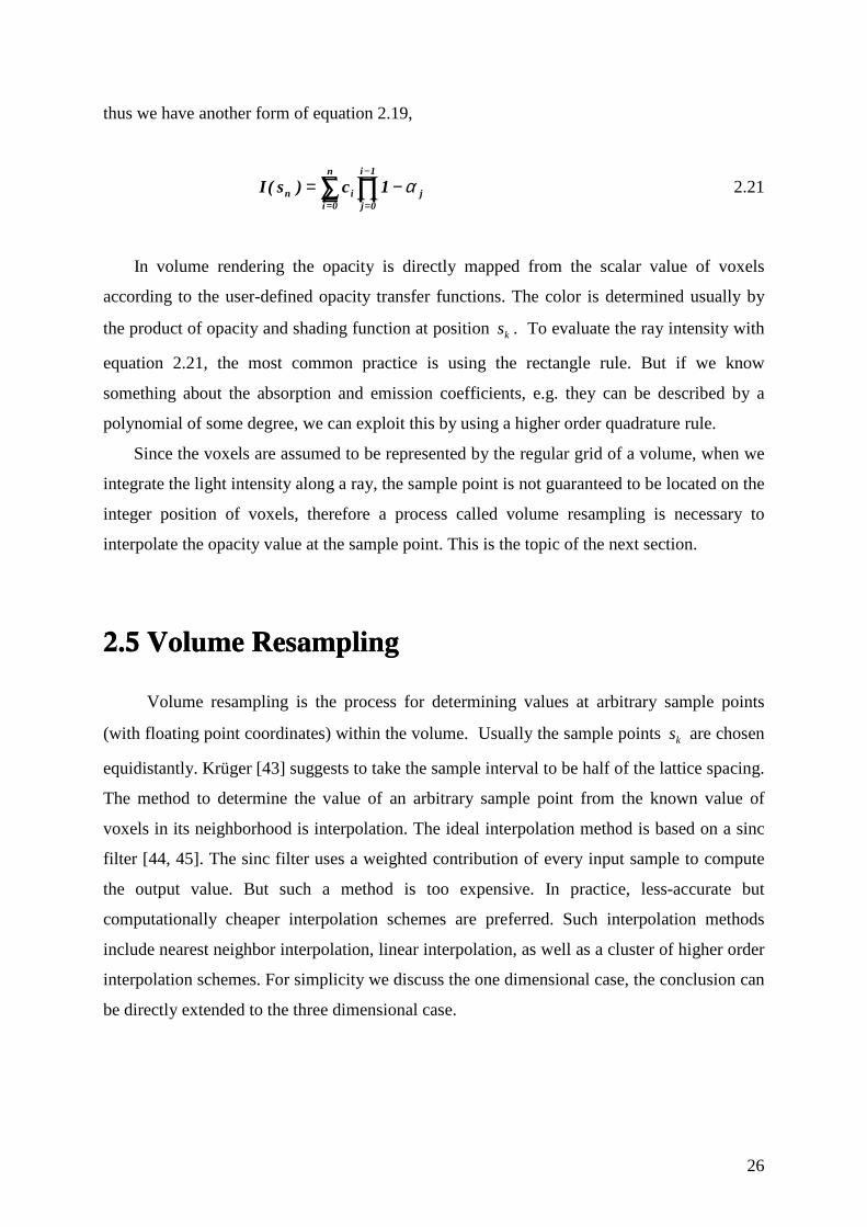
thus we have another form of equation 2.19,

∑ ∏=

−

=

−=n

0i

1i

0jjin 1c)s(I α 2.21

In volume rendering the opacity is directly mapped from the scalar value of voxels

according to the user-defined opacity transfer functions. The color is determined usually by

the product of opacity and shading function at position ks . To evaluate the ray intensity with

equation 2.21, the most common practice is using the rectangle rule. But if we know

something about the absorption and emission coefficients, e.g. they can be described by a

polynomial of some degree, we can exploit this by using a higher order quadrature rule.

Since the voxels are assumed to be represented by the regular grid of a volume, when we

integrate the light intensity along a ray, the sample point is not guaranteed to be located on the

integer position of voxels, therefore a process called volume resampling is necessary to

interpolate the opacity value at the sample point. This is the topic of the next section.

2.5 Volume Resampling

Volume resampling is the process for determining values at arbitrary sample points

(with floating point coordinates) within the volume. Usually the sample points ks are chosen

equidistantly. Krüger [43] suggests to take the sample interval to be half of the lattice spacing.

The method to determine the value of an arbitrary sample point from the known value of

voxels in its neighborhood is interpolation. The ideal interpolation method is based on a sinc

filter [44, 45]. The sinc filter uses a weighted contribution of every input sample to compute

the output value. But such a method is too expensive. In practice, less-accurate but

computationally cheaper interpolation schemes are preferred. Such interpolation methods

include nearest neighbor interpolation, linear interpolation, as well as a cluster of higher order

interpolation schemes. For simplicity we discuss the one dimensional case, the conclusion can

be directly extended to the three dimensional case.

27

2.5.1 Nearest Neighbor Interpolation

The nearest neighbor interpolation is the most simple interpolation method. It has an

order of zero. It simply assigns the value of the nearest grid point in the neighborhood to the

sample point. The advantage of the nearest neighbor interpolation is its low computational

complexity, since the only computation is to determine the address of the nearest neighbor by

rounding the coordinates of the sample point. For example, the nearest-neighbor-interpolated

value for a sample point located at (43.22, 28.90,118.72) will be equal to the value of the

voxel with location (43, 29, 119).

The volume rendering results generated by using nearest neighbor interpolation are

however of low quality, i.e. objects in the rendered image have a jagged appearance. The

reason is that the interpolation function for the nearest neighbor interpolation has a stair-like

form (figure 2.12). It is piecewise constant, not continuous.

Figure 2.12 The nearest neighbor interpolation function. The function is not continuous butpiecewise constant and has a stair-like form.

2.5.2 Linear Interpolation

Linear interpolation is a first-order interpolation method. As shown in figure 2.13, this

interpolation method evaluates the value of a sample point by summarizing the contribution of

two neighboring grid points, PL and PH. The contribution of the grid points is weighted

linearly according to their distance to the sample point, as given in equation 2.22.

LHint P)m1(PmP −+⋅= 2.22

To be more efficient, we can avoid one redundant multiplication operation in equation 2.22 by

rewriting it as follows:

n-0.5 n n+0.5 n+1 n+1.5 n+2 n+2 5 x

f(x)

Pn+1

Pn

Pn+2

28

LLHint P)PP(mP +−⋅= 2.23

Here the weight m is the difference between the address of the sample point and that of the

lower grid point PL. The location of the lower grid point PL is determined by truncating the

decimal part of the sample address. The other grid point PH can be found by simply increasing

the coordinate of grid point PL by one.

Figure 2.13 The linear interpolation function. The function is continuous, but its firstderivative is discontinuous.

The image quality using the linear interpolation is better than the nearest neighbor

interpolation. However, its computational complexity is much higher than the nearest

neighbor interpolation, because one more grid point must be addressed in addition to the

algebraic operations to summarize the contribution of the two grid points.

2.5.3 High Order Interpolation

Higher order interpolations, like the cubic spline interpolation and tri-point

interpolation, use higher order interpolation functions.

The cubic spline interpolation uses the following cubic spline function:

≤≤−⋅+⋅−⋅≤≤+⋅+−⋅+

=2x1t4xt8xt5xt

1x01x)3t(x)2t()x(f 23

23

spline . 2.24

n n+m n+1 n+2 x

f(x)

Pn+1

f(n+m)

Pn

Pn+2

m

29

where the parameter t is used to change the behavior of this function. A value of t=-0.5 has

been proved to be a good choice for image resampling [46]. Four grid points are necessary to

evaluate the value of a sample point using the following formula:

4spline3spline2spline1splineint P)m2(fP)m1(fP)m(fP)1m(fP ⋅−+⋅−+⋅+⋅+= 2.25

The cubic spline interpolation is very expensive, since it requires visiting four

neighboring grid points, four multiplication, and six additions/subtractions in addition to four

expensive evaluations of cubic spline functions. Although it overcomes the discontinuity of

the first derivative of the linear interpolation function, Bosma et al. [47] and Marschner et al.

[45] have reported that the image quality is not necessarily improved. The reason is that the

cubic spline function has an overshoot at the sharp edges [48].

Tri-point interpolation is a cheaper high order interpolation method. It requires only

three grid points and uses the following piecewise quadratic function:

≤≤+−

≤≤+−=−

23

x21

89

x23

x21

21

x043

x)x(f

2

2

intpotri . 2.26

The value of the sample point is calculated with the following formula

223intpotri21intpotriint P)PP()m23

(f)PP()m21

(fP +−⋅−+−⋅+= −− . 2.27

The tri-point interpolation function has a continuous first derivative, and it does not

suffer from the overshoot of the cubic spline function. Nevertheless, the value of the tri-point

interpolation function at x=0 is 43 , so the value of the sample point located at the grid point

will not be identical to the original value at the grid point. As a consequence, the rendered

image is a little vaguer than using other interpolation methods [47].

A comparison of volume interpolation methods can be found in [49].

In volume rendering, the high rendering speed and image quality are two main ultimate

goals when designing a volume rendering system. As volume resampling is the most often

repeated operation, the interpolation scheme for the resampling should be computationally

cheap. Higher order interpolations, like cubic spline interpolation and tri-point interpolation,

30

are too expensive, so they are rarely used. The nearest neighbor interpolation is very fast, but

it suffers from severe image quality degradation, and it is therefore rarely used as well. The

linear interpolation can provide very good image quality for most of the applications and its

computational complexity is relatively low, so it is the most widely adopted interpolation

method for volume resampling [49]. In volume rendering, the interpolation is executed in all

the three axes of the three dimensional space, therefore the linear interpolation in 3D volume

space is called tri-linear interpolation. In the following sections, if without specification, when

we talk about sampling/resampling, we are implying the tri-linear interpolation based

sampling.

2.6 Shading Estimation for Volume Rendering

Shading simulates the illumination of lights on objects. A good shading function helps

highlighting important aspect of hidden information in volume data or producing appropriate

perceptual cues.

In computer graphics different illumination models have been developed. They can be

classified into two types: local illumination models and global illumination models. In a local

illumination model only light that is directly reflected from a light source via a surface to the

viewer is considered. No account is taken of any light that is incident on the surface after

multiple reflections between other surfaces. In a global illumination model, the reflection of

light from a surface is modeled as in the local model with the addition of light incident on the

surface after multiple reflections between other surfaces. This is obviously a more

computationally intensive method than using a local model, but more realistic images are

obtained.

Since the purpose of volume rendering is to present the shape of objects in volume data

set instead of correct photo-realism [6, 50], simpler local illumination models, which

considers no multiple reflections between other surfaces, are preferred in volume rendering.

In fact, during the development of the volume rendering equation, we have assumed that

there is no multiple scattering.

The most popular local illumination model is the Phong model [51, 52]. The Phong

model is a simple empirical model, but it provides simple and fast methods for calculating the

surface intensity at a given point, and produces reasonable good results for most scenes.

31

2.6.1 Phong Shading Model

The Phong model integrates three types of reflection, i.e. ambient reflection, diffuse

reflection and specular reflection. We discuss them respectively in the following.

/ Ambient reflection:

Ambient reflection approximates the indirect diffuse reflection (or diffuse

interreflections), which is the radiance coming from a source, being reflected to a surface,

then reflected to another surface, etc, and finally to the viewer. Some people just call it

environment reflection. This environment reflection is simply assumed to have uniform

intensity in all directions. The intensity of ambient reflection is proportional to the local

properties of the object, which is modeled by a constant ak , called ambient reflection

coefficient. Let the intensity of ambient light be aI . The intensity of ambient reflection can be

evaluated by

aaamb IkI ⋅= . 2.28

with 1k0 a ≤≤ .

0 Diffuse Reflection

Diffuse Reflection approximates light coming directly from a source to a surface and

then being reflected to the viewer. Like ambient reflection, the diffuse reflection is scattered

with equal intensity in all directions, independent of the viewing direction. The diffuse

reflection is governed by the so called Lambert’s cosine law. Lambert’s law states that the

radiant energy from a unit surface area dA in any direction φ relative to the surface normal is

proportional to φcos ( see figure 2.14).

Figure 2.14. Diffuse reflection model.

φ

N1

φ

L2

dA

dA⋅cosφincident light

32

If N3

is the unit normal vector of a surface and L4

is the unit direction vector from the

position we considered on the surface to the point light source, then φcos is given by the

scalar product of N5

and L6

. The diffuse reflection is then

)LN(IkdI idattdiff

77⋅⋅⋅⋅= . 2.29

where dk is the diffuse-reflection coefficient, or diffuse reflectivity, iI is the light reaching

the local surface element, attd is the distance attenuation factor which is inversely proportional

to the square distance between the location of the reflection event and the light source.

8 Specular reflection

The specular reflection simulates the bright spot, which is called specular highlight, on

a shiny surface. For ideal specular reflection, the angle of specular reflection equals the angle

of incidence (figure 2.15), and the reflected intensity is non-zero only in the specular

reflection direction.

Figure 2.15. Specular reflection for Phong shading model.

Let R9

be the direction of specular reflection and V:

be the direction of the viewer, then

for an ideal reflector the specular reflection is visible only when R;

coincides with V<

. For real

objects (not perfect reflectors) the specular reflectance can be seen even if V=

and R>

do not

coincide, i.e., it is visible over a range of α values (or a cone of values). The shinier the

surface, the smaller the α range for specular visibility. So a specular reflectance model must

have maximum intensity at R?

, with an intensity which decreases as α increases. In the Phong

N@

RA

VB

LC

33

illumination model this is modeled by a power n of the scalar product between the viewer

direction vector VD

and the reflection vector RE

. A large n (>=200) is used for a shiny surface

and a small n for a dull surface. The specular reflection is also a function of the incidence

angle θ. An example is glass which has almost no specular reflectance for θ = 0 degrees but a

very high specular reflectance for θ > 80 degrees.

A full specular reflectance function is the Bi-directional Reflectance Distribution

Function (BRDF) [36, 41]. Since for many materials the BRDF is approximately constant, the

Phong model describes it with a constant term sk , called specular coefficient. sk is

independent of the wavelength of incident light. The specular reflection is evaluated with

nisattspec )RV(IkdI

FF⋅⋅⋅⋅= . 2.30

The whole reflected intensity for Phong shading is given by

λλλλspecdiffa IIII ++= . 2.31

where λ indicates wave lengths. Usually the whole spectrum of visible light is approximated

by many wave lengths for which specific intensities should be calculated independently.

Mayer [53] found that for most applications a set of four carefully chosen wave lengths

provides a good balance between cost and accuracy. Nevertheless, the most popular color

model in computer graphics is the RGB-model, which relies on only three wave lengths, iλ

with i={ read, green, blue} . A main advantage of the RGB-model is that a triple of RGB-

intensity can directly be used to show that particular color on a three-gun color CRT. In

volume rendering, however, except using the RGB-model, the image is also often rendered

with only one color channel, which is displayed as image with 256 grayscales. We support

both the RGB-model and 256-grayscale model in our rendering program.

2.6.2 Gradient Estimation

To calculate the illumination using the Phong model, the surface normal should be

known. Unlike the polygon-based surface graphics where the surface normal is stored with

the vertices, in volume rendering the surface normal at any sample point in the volume is

defined to be a unit vector parallel to the local gradient of the voxel scalar value v(x,y,z):

34

)z,y,x(v)z,y,x(v

)z,y,x(N∇∇=

G 2.32

Usually the gradient is approximated using the central difference gradient operator,

[ ]

[ ]

[ ] k)1z,y,x(v)1z,y,x(v21

j)z,1y,x(v)z,1y,x(v21

i)z,y,1x(v)z,y,1x(v21

)z,y,x(v

H

H

H

⋅−−++

⋅−−++

⋅−−+=∇

2.33

The computation cost for the normal calculation is therefore 7 addition operations, 6 floating-

point multiplication, 4 floating-point divisions and one square root evaluation. Additionally,

the gradient estimation needs access to 6 voxels in the neighborhood of the sample point. This

will generate a speed bottleneck for volume memory when the volume size is large. To

improve performance, simplified methods which access less voxels during estimating the

gradient can be used. For example, Pfister proposed the sheared trilinear-interpolation for

gradient estimation in the Cube Projects [54, 55]. Hesser [50] suggested using only two

gradient components for shading calculations by assuming that the rays are parallel to the

image slices. In general, however, the image quality will suffer from such simplifications [50,

54, 56].

Since the gradient estimation is one of the main time-consuming routines in the

rendering process, an alternative method is usually used to reduce the operations necessary for

the gradient estimation. Namely, instead of estimating the gradient on-the-fly, the gradient for

each voxel is precomputed and stored with the voxel, thus the expensive gradient estimation is

replaced by the cheaper memory read-out. A main disadvantage of this method is its large

memory requirement, because all three components of the gradient are floating point

numbers. To overcome this disadvantage, the precomputed gradient vectors can be encoded in

a lookup-table (LUT) which is indexed with a convenient integer [6, 57, 58]. One thing that

must be mentioned here is that the precomputed gradient can only be used for the case that the

opacity mapping stays unchanged during the feedback-loop of volume visualization. Since in

our interactive implementation the opacity transfer function is changed frequently to allow

revealing different structures in the volume, the precomputed gradient should be updated

35

whenever the opacity transfer function is changed. The operation to update the precomputed

gradient is computationally expensive, since the whole volume must be traversed. We

therefore do not use this strategy in our volume rendering algorithms.

2.6.3 Shading Calculation

Like volume resampling, the efficiency of shading calculation is also a decisive factor

which significantly affects the performance of a rendering system. Since shading calculation

is required for each sample point, it is an operation that is repeated with the same frequency as

the resampling operation. Therefore reducing the computational complexity for shading is

also an approach to accelerate volume visualization.

In volume rendering, instead of using the complex physical-based models, the

computationally cheap empirical shading models like the Phong model are commonly used

for shading calculations. In some cases even more cheaper shading models, e.g. simple

ambient shading are used, as often seen in 3D texture mapping-based rendering schemes.

By making some assumptions to simplify the lighting model, the Phong shading could

be further simplified. For example, Lacroute made two assumptions in his implementation of

the shear-warp based volume rendering software package, VolPack. First, the light direction

vector LI

is assumed to be constant for all voxels. This assumption is valid when the light

source is far enough from the volume. Second, the viewing direction vector VJ

is also assumed

to be constant. For parallel projection, the projection direction is taken as the viewing

directing. For the perspective projection, the direction of the central viewing ray is taken as

the viewing direction. This assumption, however, may lead to incorrect specular highlights,

especially when the viewer is close to or inside the volume.

In our rendering system we do allow users to do data-walk-through to fully explore the

volume data, and we also simulate volume deformation by deforming viewing rays [59, 60],

the global assumptions for the tabulation of shading functions are therefore not applicable.

Instead, our algorithms calculate the shading function on-the-fly.

2.7 Chapter Summary In this chapter we discussed the basic aspects of volume rendering. We discussed the

difference between polygon-based surface rendering and volume rendering in terms of object

presentation and the visualization process. As the theoretical background of this dissertation,

we derived the standard volume rendering equation beginning with the transfer equation. We

36

also analyzed two basic operations in volume rendering, namely volume resampling and

shading calculation. We discussed these two operations in this chapter instead of explaining

them elsewhere when we discuss detailed rendering algorithms, since they are the most

common and kernel parts of any rendering algorithm.

Now after having explained the background knowledge of volume visualization, in the

next chapter we will study more detailed techniques used in volume rendering, such as

existing volume rendering algorithms and optimization techniques.

37

Chapter 3

Volume Rendering Algorithms

Volume rendering is a well-known time-consuming process. To achieve interactive volume

rendering, three basic strategies can be taken, 1) utilizing special-purpose hardware to handle

the most computational intensive parts of volume rendering; 2) taking advantage of

parallelism; 3) reducing the complexity of the rendering process with efficient volume

rendering algorithms. In this thesis we only consider the third strategy, i.e. improving the

interactivity of volume rendering through algorithmic optimization, which is the most flexible

approach. E.g. it can be combined with the other two approaches to reduce the demands on

computing power, or be implemented alone in the pure software-based volume rendering

systems which will be finally feasible to provide real-time volume rendering on general

desktop PCs as the result of the steady increase of their computing power [61]. This chapter is

about the early work on volume rendering algorithms and the volume rendering accelerating

techniques.

38

3.1 Existing Volume Rendering Algorithms

Traditionally, volume rendering algorithms can be classified into two types: object order

algorithms and image order algorithms according to whether the main rendering loop is

ordered by volume space or image space. Texture mapping and splatting algorithms are two

typical object order rendering algorithms. In object order rendering algorithms, the volume is

traversed in an order of decreasing or increasing distance from the observer, thus the space

coherency can be fully exploited. On the contrary, the image order based methods, like ray

casting, follow single rays originated from pixels on the imaging plane, leading to irregular

traversal of voxels. Although in the image order algorithms the space coherency is not as

efficiently applicable as in object order based methods, they can be accelerated by early-ray-

termination [62] or adaptive refinement algorithms [63, 64]. There exist also hybrid rendering

algorithms which benefit from both the advantages of image order and object order

approaches, such as the shear-warp algorithm [6, 65] and the Active-Ray method [66]. We

will discuss the most typical volume rendering algorithms and their advantages and

disadvantages in implementation.

3.1.1 The Splatting Algorithm

Splatting algorithms [67, 68, 69, 70] traverse all voxels in a storage order and calculate

what contribution these voxels have to the final image. Each voxel is interpreted as an energy

source which distributes its energy over a certain area (figure 3.1). This has the same effect of

splashing a snowball at a glass plate: in the splashing center the contribution is high and, the

volume data

image plane

voxelfootprint on image

Figure 3.1 Volume Rendering by Splatting.

39

more distant to the center, the lower the contribution will be. That is why this method is

known as splatting.

The distribution of a single voxel’s energy is determined by a reconstruction filter. For

parallel viewing, the kernel of this filter can be a 2-dimensional circular kernel (usually a

Gaussian) that can be calculated once for all voxels. In perspective viewing, this kernel has to

be 3-dimensional. It is projected into the image to obtain the distribution of a voxel’s energy

for the given perspective. The result of this projection of a 3D kernel is called a footprint.

Usually there is not necessarily a pixel at the center of the projected voxel (the center of the

footprint). After the kernels or footprints have been determined, the color and opacity of the

voxels are convoluted with them. The attenuated color and opacity of the voxels are then

projected into the image plane and blended with the information stored in the frame buffer.

The computation is processed by virtually "peeling" the object space in slices, and by

accumulating the result in the image plane.

The main advantage of the splatting algorithm is that the high space coherence can

decrease the frequency to change memory pages and thus improves the cache efficiency

thanks to its regular volume traversal in storage order. In addition, fast splatting can be

achieved by using hardware-assisted Gouraud-shading methods (called coherent projection)

as suggested by Laur [68] and Wilhelms [69] etc. Besides, because the splatting algorithm

slices the volume data set one plane after another, it is suitable for efficient parallel

implementation [71, 72].

However, it is difficult to implement a splatting kernel that is not only efficient, but also

can simultaneously produce high quality images. Accurately computing the resampling

weights of the footprint is expensive due to the dependence of footprint on view-settings.

When the view-settings are changed, the footprint must be scaled, rotated, and transformed

correspondingly. Moreover, in a perspective view, the footprint changes from voxel to voxel.

To solve this problem, approximation approaches such as precomputed lookup tables for the

resampling filter can be used which achieve faster rendering at the cost of losing image

quality [67, 73].

3.1.2 3D Texture Mapping

3D texture mapping [74, 75, 76] is also an object space volume rendering method.

Instead of processing only one voxel at a time, it converts the original data into a 3D texture

map in form of slices (figure 3.2), then the specialized texture hardware in modern graphics

system performs the slice rendering and compositing very quickly [26, 77].

40

Figure 3.2 Slices through the volume data in the parallel projection. The volume on the left isaligned parallel to the image plane. On the right the volume is rotated. In both cases the slicesare perpendicular to the viewing direction (by A. Gelder et al. [74]).

3D texture mapping takes two major steps: (1) create the texture map and (2) render

the slices. During the creation of the texture map, a plane to be rendered is assigned to the

center of each slice (with thickness). Each plane has a representation color intensity and

opacity associated with a slice. The thickness of each slice ∆d is the total distance covered by

the stack of planes divided by the number of planes. The color emission per unit distance and

the opacity per unit distance are assigned to the data at each point by the transfer function.

After evaluating the integration of color and opacity through the thickness of the slice, each

voxel in the data is assigned to its color and opacity, which are converted from floating point

values into integers in an appropriate range for storage in the texture map. Whenever the

transfer function or the number of slices is changed, the texture map entry needs to be

recalculated.

Once the 3D texture is created, the volume can be rendered by applying the texture to

the parallel square planes and thus building up a stack of slices through the texture (see figure

3.2). The square planes are then drawn from back to front. Here the orientation of the square

planes must remain fixed in the image space, parallel to the projection plane, with their

normals towards the viewer. Otherwise, if the squares were viewed oblique, their interval

along the view direction would not be ∆d, and the color and opacity obtained from the texture

map would not be correct. Moreover, it is impossible to compensate for this discrepancy,

because the color and opacity are nonlinear functions of ∆d. The similar problem occurs for

the perspective view of volume data. To correctly render a volume from a rotated viewpoint

View directionView direction

slices

volume data

41

(figure 3.2 right), the square planes are kept stationary in the image space. Instead, only the

texture-space coordinates of the corners of the squares are rotated using the texture matrix,

which is part of the graphics systems [74]. To render a perspective view of the volume,

concentric shells instead of square planes are used to guarantee that the sample positions of

the texture are equidistant (figure 3.3) .

Figure 3.3 Concentric spheres for a perspective projection in 3D texture mapping.

Since the expensive operations like tri-linear interpolations and clipping are

implemented in the hardware, the 3D texture based volume rendering can speed up the

rendering process by more than one order of magnitude [75].

One of the main disadvantages of most 3D texture based volume rendering schemes is

that they do not support complex shading calculation. Instead, the color is mapped directly

from the scalar value through a color transfer function. Gelder et al. [74] developed a

gradient-based shading technique. The technique depends on quantified gradients and a

precomputed lookup table. However, the performance suffers considerably from the changes

of volume orientation and light position, because the lookup table should be updated

whenever the volume is rotated or the light is assigned to a new position. The overhead due to

the updating of the lookup table is proportional to the size of the volume. Recently, more

flexible shading schemes for 3D texture mapping based volume rendering have been proposed

[78, 79]. Instead of calculating the lighting on the host, only the components of the gradient

vectors are calculated in advance and saved as color components in the 3D texture. By taking

advantage of the color matrix extension of OpenGL 1.2, the light direction can be processed

to form a matrix that when multiplied by the texture color components (now containing the

components of the normal at that point), will produce the dot product of the two. Since the

42

color matrix is part of the pixel path, this processing can be done when the texture is loaded.

The 3D texture contains lighting intensities as that in Gelder [74], but the dot product

calculations are done in the pixel pipeline, not in the host. Hence, a change of light source (or

viewer position, if specular lighting is desired) does not require the volume data to be

reprocessed.

Another main constraint for 3D texture mapping based volume rendering is the limited

amount of texture memory. This limit can be partly solved by e.g. paging of textures [23, 80],

using texture map hierarchy [81]. However, such methods either severely hamper the

interactivity when rendering volumes whose size exceeds the physical texture memory, or

degrade the image quality.

3.1.3 Ray Casting Algorithms

Ray casting is the most attractive method for volume rendering because of its superior

image quality compared to others. It is an image-order method, because the traversal order of

the related voxels is determined by pixels on an image plane.

At the initial step, parameters like viewer position, viewing direction, light etc. are defined

by the user. A view transformation matrix is generated according to the view-settings.

To evaluate the intensity of a pixel for the parallel projection, a ray is cast directly from

the pixel on the image plane into the virtual scene with the same direction as the principal

viewing axis; for the perspective projection, a ray is originated from the viewer passing

through the pixel on the image plane. The ray is then transformed from image space to object

space. This transformation is done by inverting the viewing matrix.

Then the cast ray is checked to see if it intersects with the volume. If the ray does not pass

through the volume, it is simply skipped over and the pixel is assigned with a default color,

usually black. Otherwise the volume is sampled along the ray (see figure 3.4). At the sample

points the opacity and shading are calculated by the user-defined opacity transfer function and

the selected shading model (usually Phong illumination model). Then the contribution of each

sample point is combined as described by the equation 2.21 (the volumetric composition

equation). Note that the only elements that contribute to the ray intensity are the sampled

points along the ray. This differs it from ray tracing, since shadows or reflections are not

generated by using this method (volumetric ray tracing methods do exist, for such methods,

reader is referred to [6, 50, 82, 83, 84]).

43

Figure 3.4 Ray casting (parallel projection). The cast rays are checked to see if they intersectwith the volume. Volume is sampled along the rays which pass through the volume.

The image quality and rendering speed can be quite different according to how the

volume is navigated along a ray and how the sample values are determined.

The fastest approach to evaluate a sample value is using a nearest neighbor interpolation

(also called point interpolation). While navigating along the cast ray, we can use the 3D

digital differential analyzer (DDA) [85], which works the following way: the long dimension

is incremented for each pixel, and the fractional slope is accumulated. The algorithm keeps

the accumulated distance traveled from the origin to the x-,y- or z-value of the currently

selected voxel (see figure 3.5 for a 2D-equivalent example). The gray square in the image

represents the currently selected voxel. The gray arrow stands for the ray direction. The green

line shows the distance from the origin to the x-value of the currently selected voxel (dx). The

red line shows this for the y-value (dy). DDA determines, based on whether the dx or the dy is

bigger, if the next pixel (voxel) is respectively one step up or one step to the right. In the

example ( figure 3.5 left), the next step will be to the right, since the green arrow is not as

long as the red one: dy>dx. One problem with the DDA is that in some special cases the

structure in the volume could be leaped over without sampling it, as seen in figure 3.5 right.

image plane volume data

rays

44

Figure 3.5 The digital differential analyzer(DDA) for volume navigation. The image on theleft shows how the next voxel is selected along the ray. The right image demonstrates themissing of object voxels (red ones) because the DDA allows the jump to the diagonal adjacentvoxel( 26 connect-path), here the green points are the selected sample points.

An improvement to the DDA is using the 6-connected path Bresenham algorithm [86, 87].

With this algorithm, the sample points can only travel from one voxel to one of the 6-

connected neighbors, thus the leap-over of an object voxel is avoided, as seen in figure 3.6.

Figure 3.6 The 6-connected path Bresenham algorithm for volume navigation.

Since the nearest neighbor interpolation could result in stair-like artifacts, it is usually

only used to provide a fast preview of volume data and to adjust rendering parameters.

In ray casting, the most frequently used method to evaluate a sample point is using tri-

linear interpolation. When using tri-linear interpolation, the volume is equidistantly traversed

along the ray, thus the coordinates of the sample points are not integers, but floating point

45

numbers. This interpolation algorithm uses the same eight points as the mean-density method

(which simply averages the density value of eight neighboring voxels for speed’s sake), but

does a weighted average of the density of eight neighboring voxel values. This assumes that

the slope is constant between the voxels. While working with a low-resolution model, this

will create inaccuracies, but as the resolution increases the slope will appear to be more

constant—any differentiable function will appear linear when examined on a small enough

scale. The tri-linear interpolation based equidistant sampling along the ray can produce quite

good image quality for most applications.

The main disadvantage of ray casting is that it is computational intensive. Many

operations involved in the rendering process, like shading calculation and tri-linear

interpolation, are very expensive. In addition, compared to the object space algorithms, the

addressing arithmetic calculation in ray casting is a significant overhead, even when we use

the simplest point-interpolation.

Ray casting also represents a heavy burden to the memory system. Since the traversal of

a relatively large part of the data set is necessary for every ray, this will decrease the

efficiency of the cache system, therefore memory bandwidth requirement is high for

interactive applications.

Ray casting can be accelerated by different methods like adaptive image refinements,

early-ray-termination and space-leaping etc.

3.1.4 Hybrid Algorithms

As discussed in the previous sections, the object space algorithms, such as the splatting

algorithm, can take advantage of simplified address arithmetic and coherency in volume data

because the volume in such algorithms is traversed in storage order. On the other hand, image

space algorithms, e.g. ray casting, can also be accelerated by techniques like early-ray-

termination and produce images with high quality usually not achievable by using object

space algorithms [88]. To combine the advantages of both object space algorithms and image

space algorithms, people developed several hybrid algorithms. Typical hybrid algorithms

include the shear-warp algorithms and the Active-Ray method [66].

Active Ray was implemented on parallel computing environments. It divides the

volume data into cells that are distributed randomly to processors. Rays are intersected with

the cell boundaries and are placed in a queue associated with the cell they intersect first.

These cells are brought into memory by demand in a front-to-back order. Rays queued at a

46

cell that was brought into the processor’s memory are advanced in the cell, they either stop

due to opacity saturation (early-ray-termination), or are queued at the cell they enter next.

The idea of a ray queue is adopted by Vettermann et al. [8] in their Volume Rendering Engine

(VGE) architecture. In VGE each rendering pipeline is augmented with a ray queue. By

assigning a thread for each ray whose information is stored in the ray queue and using a ray

bundle of 8×8 rays to exploit the space coherency, they minimized the redundant wait cycle of

the rendering pipeline and the memory bandwidth overhead, thus they achieved real time

frame rates for ray casting of 2562x128 volume data.

The shear-warp algorithm is based on the factorization of viewing transformation matrix

[6, 65, 89, 90]. Klein Küber and Ylä-Jääski [91] used the shear-warp factorization to simplify

projecting volume into image plane, thus reducing the amount of addressing arithmetic

required by ray casting. Cameron and Undrill’s algorithm [92] uses the shear-warp

factorization to construct volume renderers for a SIMD massively parallel multiprocessor

which benefits from the regular communication patterns between the processors. Schröder

and Stoll’s algorithm [93] also uses the shear-warp factorization in their SIMD parallel

implementation. In their algorithm, however, the ray information instead of the volume data is

transferred between processors. Lacroute and Levoy [6][94] extended the shear-warp

algorithm by introducing a factorization for perspective projections and several accelerating

approaches to improve performance.

The viewing transformation matrix in the shear-warp algorithm is decomposed into two

concatenated matrixes, one for the shear transformation of the volume, and the other for the

warping of the intermediate projection. In Lacroute and Levoy’s implementation, the shear-

warp algorithm is therefore mapped to two separate steps. In the first step, the volume is

sheared parallel to the set of slices that is most perpendicular to the viewing direction. For

parallel projection the shear transformation needs only a simple translation of each slice,

while for the perspective projection the slices are scaled in addition to the translation (see

figure 3.7). Then the sheared slices are resampled and composited into an intermediate image.

Since the scanlines in the sheared slices are parallel to the intermediate plane, the volume can

be resampled using only a 2D interpolation instead of a 3D interpolation by letting the sample

distance be the same length of slice distance. Furthermore, for the parallel projection all

voxels in a given slice of the volume have the same resampling weights, so the sampling

weights can be precomputed and reused for every sample point. Thus the sampling in the

shear-warp algorithm is very efficient.

47

In the second step, the intermediate image is warped into the final image by using the

factorized warping transformation. The warping of the intermediate image is not expensive,

because it is a 2D operation.

As a hybrid algorithm, it has some properties of the object space algorithm, for example,

the volume is traversed in the storage order. The shear-warp algorithm bears some similarities

to the 3D texture mapping based technique, in that the volume is presented as a series of

parallel slices (planes) for rendering purposes. However, in the texture mapping

implementation, the planes are parallel to the projection plane, and usually oblique to the

volume. In the shear-warp method, the planes simply correspond to slices in the original

volume and are perpendicular to the principal axis, which are parallel to the view direction.

Meanwhile, the shear-warp algorithm can be considered as a skewed form of ray casting.

Acceleration methods for ray casting, such as early-ray-termination, can also be used by the

shear-warp algorithm. But the image quality of shear-warp is not as good as that of ray

casting, which is the result of using a 2D interpolation kernel during volume resampling and

an extra 2D resampling of the intermediate image while generating the final image.

Figure 3.7 Shear-warp transformation. a) Shear-warp for parallel projection, b) Shear-warpfor perspective projection.

Image plane Image plane

intermediateimage composite

shear slicesviewing rays

Image plane Image plane

intermediateimage

shear and scale slices

composite

warp

viewing rays

a)

b)

warp

48

3.2 Volume Rendering Accelerating Techniques

Volume rendering is a very computationally expensive process. The complexity of brute

force volume rendering algorithms is proportional to the volume size. Currently, a volume

with 2563~5123 voxels is regarded as middle size. Gigabyte volume data has been used in

some applications. When using a splatting algorithm, the rendering for a 2563 volume data

requires approximately 1.8×109 floating point operations for rendering one frame, and

5.4×1010 for real time rendering (30 frames/second). For other algorithms the required

computation is close to this estimation [1]. This is far beyond the available processor

performance of the most advanced common desktop computer systems (see figure 3.8).

Therefore accelerating techniques are necessary in order to decrease the computation

complexity for interactive volume rendering.

Figure 3.8 The synthetic performance benchmarks of different processors from AMD andIntel. The numbers behind the CPU names stand for CPU clock frequency, bus frequency andmemory frequency separately.(http://www.zdnet.de/techexpert/artikel/tests/cpu/200102/cputop_00-wc.html)

49

Different accelerating techniques have been developed in the last decade. Common

methods include coherency accelerating approaches, adaptive sampling techniques,

presentation acceleration, early-ray-termination, and precomputation etc. Usually the

performance gain achieved by a single acceleration technique is limited and depends often on

the data feature. One common practice is to combine several acceleration techniques in one

algorithm to achieve higher speedup [1, 62, 95] and minimize the dependence of performance

on the data feature. To be clear, though, we discuss different techniques separately.

3.2.1 Coherency Acceleration

• Image space coherency

The adaptive image refinement algorithm [63, 64] exploits the coherency in the image

space. It can only be used by the ray casting algorithm. The adaptive refinement first

generates a coarse image by ray casting only a subset of the screen pixels, e.g. every other

column and every other row. The image is refined by checking the image gradient in the

coarse image. If the gradient is below a user-defined threshold, the empty pixel residing

between the pixels in the coarse image is assigned a value by linear interpolation. Otherwise,

additional rays are cast to solve the ambiguity in the areas with high gradient. Whether

additional rays should be cast or not is determined by the local gradient of pixel values in the

coarse image instead of in a local neighborhood in the volume space, so there is a risk of

losing details in the original volume.

• Object space coherency

In most of volume data there is high coherency between voxels. The volume rendering

can be accelerated by reducing sampling in 3D regions where voxels have uniform or similar

values.

Object space coherency is usually exploited by using hierarchical data structures like

octree [68] and k-dimensional tree [96]. For example, Laur and Hanrahan built an octree over

voxels, and computed the voxel mean values and root mean square error (RME2) at each

node. By using a user-defined error tolerance, volume can be rendered with progressive

refinement: nodes with RME2 less than the error tolerance are rendered as single “splats” . By

using such precomputed space data structures, the rendering process can be accelerated by

50

treating the splats as polygons and using hardware-assisted Gouraud-shading (called coherent

projection) [68, 96, 97, 98, 99].

Van Walsum et al. [100] exploited object space coherency for ray casting. His method

first samples the volume with a relatively large step along a ray. The difference between the

sample values is checked on-the-fly. If the difference between two adjacent samples is too

large, the sample distance is shortened till an appropriate sample step is found. Thus the

ambiguities in the high frequency regions can be resolved. This method was extended by

Danskin and Hanrahan [95] to efficiently lower the ray casting sampling rate in homogeneous

regions or in regions with low contributions of opacity. In their implementation, they used

several pyramid data structures to encode the coherence information.

3.2.2 Presentation Acceleration

According to the volumetric composition formula (equation 2.21), when the opacity of a

voxel is zero, it will contribute nothing to the ray, including the intensity and the accumulated

opacity. The voxel with opacity value of zero is called empty voxel. For typical opacity

transfer functions the volume data contains about 70%~80% empty voxels [62, 101]. Lacroute

[94] reported that the data sets with expressed surfaces have empty voxels up to 95%. The

presentation acceleration techniques speed up the rendering process by neglecting the

operations related to the empty voxels, i.e. when there is not any non-empty voxel presented

at the neighborhood of a sample point, the ray can be safely proceeded without conducting

any of the complexity calculations like resampling and shading. In implementation, an opacity

threshold is usually used [62, 94], i.e., if thαα < , the voxel is considered to be empty.

The brute force presentation acceleration method by Levoy [62] uses a hierarchical

enumeration to describe the empty regions in a volume (see figure 3.9). He reported a speedup

factor between 2.0 and 5.0. A problem with the hierarchical enumeration based presentation

acceleration is that the navigation between different levels of the hierarchical data structure

complicates the addressing arithmetic. Similar implementations can be found in Danskin and

Hanrahan [95]. They used a pyramid to encode the empty regions in the volume.

51

Figure 3.9 Ray-casting of hierarchical enumeration (by Marc Levoy)

Space-leaping is an efficient presentation acceleration method. Space-leaping relies on a

distance transform [102, 103]. Before rendering a volume, the distance from any empty voxel

to the nearest non-empty voxel in its 3D neighborhood is determined by the distance

transform and is encoded in a distance array with the same size as the volume (see figure

3.10). The encoded distances are view-independent. This preprocessing is called distance

coding. The encoded distances are used in the rendering process to skip the empty regions

along a cast ray. Since the same addressing arithmetic can be shared between distance read-

out and voxel value read-out, the algorithm is of a high performance.

Lacraute implemented the presentation acceleration in his fast shear-warp algorithms

[94] in another way. The shear-warp traverses the volume strictly in the storage order,

scanline by scanline, therefore the empty regions in the volume is conveniently encoded with

run-length codes. The scanlines in the sheared volume are aligned with the pixel scanlines in

the intermediate image. So during the compositing stage, the run-length code can be used to

traverse the empty voxels without compositing them with the content in the corresponding

scanline segment, thus presenting a considerable performance gain.

52

Figure 3.10 Distance coding. Each voxel is assigned a distance value which is the distance tothe nearest opaque voxel in its 3D neighborhood.

3.2.3 Early-Ray-Termination

Early-ray-termination [62] is a common acceleration technique for volume rendering.

Early-ray-termination is well suitable for being implemented in a ray casting algorithm,

because it works in front-to-back order. As a ray proceeds in the volume, the ray opacity is

accumulated. When the opacity reaches a threshold close to full opacity, the ray is terminated,

because the voxels lying far away are occluded and contribute very little to the ray intensity

and need not to be processed. Levoy reported that the ray casting of medical data sets by

using an opacity threshold of 0.95 (full opacity is 1.0) could achieve speedups between 1.6

and 2.2 times. Danskin and Hanrahan [95] generalized Russian Roulette [104] to implement

early-ray-termination in volume rendering. It kills off some of the ray casting calculations

according to a probability that increases with accumulated ray opacity. It returns an unbiased

average ray intensity by increasing the weight of the surviving calculations.

In principle, early-ray-termination can also be implemented in object space algorithms.

It is, however, not efficient. For example, in the splatting algorithm, the early-ray-termination

can be realized by checking each pixel’s opacity before compositing a voxel to it. However,

since the footprint of a voxel is distributed in a small area with several pixels instead of only a

single pixel, the voxel still needs to be processed unless the opacities of all pixels covered by

the footprint exceed the opacity threshold. Therefore, early-ray-termination does not reduce

the time spent traversing occluded portions of the volume. What must be made clear is that

there are actually no rays in the object space algorithm, so the counterpart of early-ray-

opaque voxel

distance value foran empty voxel

53

termination in the object space algorithm is called opacity saturation or early-splat-elimination

[88].

An improved but more sophisticated splatting algorithm was proposed by Meagher [105]

to exploit the opacity saturation in the image plane. The algorithm uses a quadtree data

structure to encode the image regions where the opacity of pixels exceeds the opacity

threshold. Meanwhile an octree is used to encode coherence in the volume space. The

algorithm traverses the octree nodes in front-to-back order and splats the voxels in each node

into the image. Before splatting, the silhouette of the octree node on the image plane is

computed by scan-converting and the accumulated opacity in the quadtree nodes that overlap

with the silhouette is checked. The voxels in the octree node is culled when the quadtree

nodes are opaque. Thus by using the octree and quadtree data structures to encode the

coherence in both object space and image space, the opacity checking of individual voxels is

avoided. Instead, an occluded octree node of arbitrary size can be culled by checking a small

number of quadtree nodes. However, the overhead required to produce the silhouettes of

octree nodes and traverse the quadtree data structure may be large compared to the rendering

time. This cancels the performance gain achieved by ignoring the occluded octree nodes.

Reynolds [65] proposed a more efficient technique for parallel projection called

“dynamic screen” . Lacroute[6, 94] adopted this technique in his fast shear-warp algorithm.

This technique is based on the observation that after the shear transformation the slices in the

volume are aligned parallel to the image plane, further, the scanlines in the slice are also

parallel to that of the image in the projection plane. In addition to using a run-length to encode

the empty runs in the volume scanlines as discussed in the presentation acceleration

technique, another run-length can be used to encode the runs of pixels with saturated opacity

values in the projection plane. The algorithm can then use both run-lengths to simultaneously

traverse the voxel scanline and the image scanline it projects onto. Since the voxel scanline

coincides with the pixel scanline in the projection plane, during the traversal, the algorithm

can use the run-length encoding of the voxel scanline to skip empty voxels and the run-length

encoding of the image scanline to skip over occluded voxels, i.e., the algorithm processes

only those voxels which are non-empty and are projected onto non-opaque pixels.

3.2.4 Preprocessing

Preprocessing is a technique widely used in volume rendering to generate repeatedly

used intermediate data, such as lookup tables (abbreviated as LUTs). Westover [73] used the

preprocessing to generate LUTs for rotation-invariant Gaussian resampling filters for fast

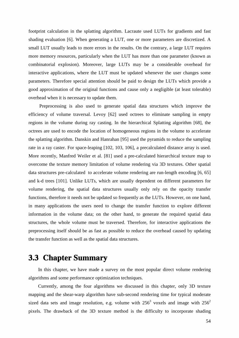
54

footprint calculation in the splatting algorithm. Lacraute used LUTs for gradients and fast

shading evaluation [6]. When generating a LUT, one or more parameters are discretized. A

small LUT usually leads to more errors in the results. On the contrary, a large LUT requires

more memory resources, particularly when the LUT has more than one parameter (known as

combinatorial explosion). Moreover, large LUTs may be a considerable overhead for

interactive applications, where the LUT must be updated whenever the user changes some

parameters. Therefore special attention should be paid to design the LUTs which provide a

good approximation of the original functions and cause only a negligible (at least tolerable)

overhead when it is necessary to update them.

Preprocessing is also used to generate spatial data structures which improve the

efficiency of volume traversal. Levoy [62] used octrees to eliminate sampling in empty

regions in the volume during ray casting. In the hierarchical Splatting algorithm [68], the

octrees are used to encode the location of homogeneous regions in the volume to accelerate

the splatting algorithm. Danskin and Hanrahan [95] used the pyramids to reduce the sampling

rate in a ray caster. For space-leaping [102, 103, 106], a precalculated distance array is used.

More recently, Manfred Weiler et al. [81] used a pre-calculated hierarchical texture map to

overcome the texture memory limitation of volume rendering via 3D textures. Other spatial

data structures pre-calculated to accelerate volume rendering are run-length encoding [6, 65]

and k-d trees [101]. Unlike LUTs, which are usually dependent on different parameters for

volume rendering, the spatial data structures usually only rely on the opacity transfer

functions, therefore it needs not be updated so frequently as the LUTs. However, on one hand,

in many applications the users need to change the transfer function to explore different

information in the volume data; on the other hand, to generate the required spatial data

structures, the whole volume must be traversed. Therefore, for interactive applications the

preprocessing itself should be as fast as possible to reduce the overhead caused by updating

the transfer function as well as the spatial data structures.

3.3 Chapter Summary In this chapter, we have made a survey on the most popular direct volume rendering

algorithms and some performance optimization techniques.

Currently, among the four algorithms we discussed in this chapter, only 3D texture

mapping and the shear-warp algorithm have sub-second rendering time for typical moderate

sized data sets and image resolution, e.g. volume with 2563 voxels and image with 2562

pixels. The drawback of the 3D texture method is the difficulty to incorporate shading

55

calculation into the rendering process, therefore the result image looks dull. Although shading

can be implemented in the 3D texture mapping, it relies on a time-consuming and view-

dependent precalculation [74]. Besides, on many machines the texture memory is limited

compared to the 3D texture volume and thereby frequent swaps of 3D volume texture in and

out of the texture memory is necessary and lowers the performance.

The shear-warp algorithm combines the advantages of both object space and image

space algorithms. Two efficient acceleration techniques, the presentation acceleration and

early-ray-termination, are easily implemented by using run-length encoding. The voxel

addressing arithmetic is also simple because of its storage order traversal of volume.

Furthermore, all optimizations are independent of the hardware architecture. Therefore the

shear-warp stands for the performance limits on single desktop computer systems. However,

the shear-warp algorithm has difficulties to simulate the walk-through of the volume, because

when the viewer is located inside the volume, there will be no single principal viewing axis

that is consistent with all viewing rays. Moreover, the rendered image is smooth because of

two sampling processes.

The splatting algorithm and the ray casting have similar performance. Usually, the

splatting algorithm produces smoother images than ray casting due to the projection of the 3D

reconstruction kernel to the 2D footprint and the anti-aliasing effect of the larger Gaussian

filter. Unlike other algorithms, which traverses the volume in storage order, ray casting has

the most expensive addressing arithmetic requiring high memory bandwidth for interactive

implementation. But the complex addressing arithmetic endows it with much flexibility. For

example, perspective projection can be implemented as easily as parallel projection; visual

hints such as depth cue can be easily realized; polygon-based models can be rendered with the

volume in the same scene [107]. We can even virtually deform the cast rays to fake

deformation of the volume (presented in chapter 6)!

Since ray casting is flexible and can generate the most appealing image, it is most

widely used in volume visualization. However, as having been discussed in this chapter, it is a

very computationally intensive process, and therefore limits its application fields, especially

where interactivity is very important. Even for the shear-warp algorithm, the interactivity is

only achieved on high-end graphics workstations [88, 94]. We have still much to do before

interactive volume rendering can be achieved on the common desktop PCs.

In the next chapter we present a new method for volume rendering acceleration.

56

57

Chapter 4

Algorithms for Exploiting Coherencein Volume Data

4.1 Introduction

Exploiting coherence is one of the most efficient approaches to accelerate volume

rendering [1]. Coherence is the quality or state of cohering, especially a logical, orderly

consistent relationship of parts. In volume data sets three types of coherence are widely

observable in terms of opacity property of voxels, they are emptiness, homogeneity and

linearity. Figure 4.1 shows a CT image which has large area of high coherent regions. In

volume rendering, however, the coherence is traditionally interpreted only as homogeneity of

voxels, e.g. voxels with same opacity value (not necessarily zero). The homogeneity in

58

volume data is usually described with hierarchical spatial data structures like octrees and

pyramids [62, 68, 95].

Figure 4.1 Coherence in volume data. a) A typical slice from the volume data jaw (2562×128).b) 3D plot of the slice with homogeneous regions color coded, the smooth transition (whichcan be linearized) between different homogeneous regions is noticeable. c) A scanline fromthe slice. Three types of coherence, i.e. transparent regions, homogeneous regions, and lineartransition regions are indicated in the curve of scalar values.

a)

b)

c)

x

grayvalue

59

The hierarchical spatial data structures can help some rendering approaches to fully

exploit the coherence in the volume data, but not all. The splatting algorithm benefits mostly

from the homogeneity encoding of volume data with hierarchical spatial data structures, since

the traversal of the volume in storage order is easy to be implemented with such data

structures without leading to complex addressing arithmetic. For the image order algorithms,

e.g. ray casting, the situation is different. If the homogeneous region is, for example, encoded

with octrees, the traversal of the ray in the octree is composed of complex horizontal and

vertical moves [108, 109]. With a horizontal move, the ray proceeds between adjacent nodes

of the same size which are immediate siblings in the octree, while with a vertical move the ray

proceeds between non-immediate siblings which requires descending or ascending the tree.

To make a move between siblings, a next-cell detection test to search the next adjacent node

along the ray is necessary [110]. Therefore, the traversal of octrees is computationally

expensive in ray casting.

To circumvent the overhead of moving up and down the hierarchical data structures, new

techniques have been developed to encode the homogeneity of volume data in more efficient

forms which simplify the traversal of the homogeneous regions during ray casting. In these

new techniques, the homogeneity information is stored in look-aside buffers [103, 111],

proximity clouds [106] or run-length encoding [6] etc.

Both the look-aside buffer and proximity cloud techniques are based on a 3D-distance

transform [103, 106]. The distance transform determines the distance from an empty voxel to

the nearest non-empty voxel in its 3D neighborhood. The difference between the look-aside

buffer and the proximity cloud is that the former uses a separate buffer of the same size as the

volume to save the distance for each voxel (both empty and non-empty), while the proximity

cloud directly replaces the empty voxel’s scalar value with the distance value marked with an

extra flag bit. Therefore it does not consume extra memory for saving the homogeneous

information. In Lacroute’s fast shear-warp algorithm, empty regions in the volume are

encoded with run-lengths in voxel scanlines. In the compositing phase the run-length is used

to precisely skip empty voxels. The success of these techniques over the hierarchical data

structure based techniques stems from their encoding schemes by which the “ leap” or “skip”

are indexed with the same indexes used for the volume data. Hence they have simple

addressing arithmetic. Nevertheless, these approaches only exploit one of the coherence types

in volume, e.g., emptiness. As figure 4.1c shows, other two coherence forms also occupy

considerable space in the volume data, therefore further accelerating of the ray casting process

will be possible if all three forms of coherence are exploited.

60

Recently, Freund and Sloan [112] proposed a homogeneous region encoding based

accelerating algorithm. Their method encodes the skip distance for every voxel in the empty

regions as well as homogeneous non-empty regions. One problem of their method is that the

homogeneity in the volume must be determined by segmenting before rendering. As we

discussed in chapter 2, the available segmentation methods are currently either not robust or

very time consuming. Besides, in their method the linear-coherence in volumes is not

considered.

In the next sections we propose two algorithms which can fully exploit all of the three

forms of coherence.

4.2 Accelerating the Shear-Warp Algorithm withScanline Coherence Encoding

4.2.1 Implementation of Earlier Shear-Warp Algorithms

In the shear-warp algorithm, the viewing matrix is factorized into two concatenated

transformation matrixes: shear transformation and warp transformation. After the shear

transformation, the voxel scanlines in the sheared volume are aligned with the intermediate

image. This means that both volume and image data structures can be traversed

simultaneously in scanline order.

To exploit the scanline coherence, scanline-based coherence data structures such as run-

length encoding [6, 113] and linked list [65] are used.

One problem introduced by the run-length encoding and linked lists is that random

access to a slice of the encoded data is impossible, because both presentations must decode

the voxels sequentially from the beginning of the data structures. In many cases, however, it is

necessary to composite the slices in inverse order, i.e., from back to front, for example, when

the volume is rotated with a large angle close to 180 degree. In such a case the sequential

traversal of the encoded volume data will lead to tremendous overhead. A method developed

by Lacroute solved this problem. His method uses three data structures to encode the volume:

a run-length array, a pointer array, and a voxel array (see figure 4.2). In the run-length array

every other entry contains the length of a run of the empty voxels. The remaining entries

contain the lengths of the intervening runs of non-empty voxels. The voxel array stores all the

non-empty voxels one by one, while the empty voxels are omitted because they are not used

61

in the rendering phase. In this way, the volume is stored in a compressed form. For each slice

there is an entry stored in the pointer array in ascendant order of slice index. Each entry has

two pointers, with one pointing to the position of the slice’s first run-length in the array of

run-lengths, and the other to the first non-empty voxel of the slice in the voxel array.

Therefore, by visiting the entry in the array of pointers using the slice index, any voxel slice

can be randomly accessed and reconstructed.

Figure 4.2 Three data structures of the run-length encoded volume (drawn after Lacroute).

However, using the data structures described above has another problem when the

viewing direction (principal viewing axis) changes considerably so that a different face of the

volume cube must be used for compositing. In this case the traversal order of scanlines needs

to be changed. To solve this problem, Lacroute used three pre-computed run-length encoding,

each for one of the three principal viewing axes. This will consume a threefold of memory.

Since in the encoded volume only the non-empty voxels are saved, as Lacroute argued, most

volume data sets have 70%-95% empty space. The total size of the encoded volume is

typically smaller than the original volume.

In the shear-warp algorithm the coherence in the image space is also efficiently

exploited by using scanline data structures. In the intermediate image, as more and more

slices are composited, more and more pixels become opaque (we say a pixel is opaque when

62

its opacity exceeds the opacity threshold for early-ray-termination). Since the voxel scanlines

are traversed simultaneously with the image scanlines, the voxels in the remaining slices

which are mapped to the opaque pixels can be skipped with the help of the run-length

encoding of continuous opaque pixels in the intermediate image. As the result of the run-

length encoding, each opaque pixel in the intermediate image is assigned with an offset value.

The offset points to the next non-opaque pixel in the same scanline. In the rendering process,

before compositing the contribution of voxels to a pixel, the offset value of the pixel is

checked. If it is non-zero, it is used to skip a run of opaque pixels behind the pixel without

sampling the corresponding occluded voxels as well as doing the compositing operations.

Unlike the run-length encoded volume data structures which are calculated in the

preprocessing stage, the intermediate image and its run-length encoding data structure must

be dynamically updated during the rendering procedure—therefore this method is called

dynamic screen by Reynolds [65]. For the sake of efficient accessing and updating, the runs

of the run-length encoding are saved as a relative offset together with the color and opacity in

each pixel. In this way the opaque pixel runs can be created or merged with adjacent runs

dynamically. The relative offset is the number of pixels from the current pixel to the next non-

opaque pixel in the scanline (figure 4.3). For the non-opaque pixel the offset equals zero.

Since it is possible to jump into the middle of a run of opaque pixels after traversing a run of

transparent voxels, storing an independent offset for each pixel in a run, not just the first pixel,

can guarantee that the opaque pixel runs can be efficiently skipped in any case.

Figure 4.3 Offsets of pixels in a scanline of the intermediate image.

By using the above data structures to encode the coherence in both voxel scaline and

image scanline, the rendering process is implemented as follows: for each slice of volume,

march through the slice and intermediate image in scanline order; for the run of the empty

voxels, skip the length of the run in both voxel scanline and intermediate image scanline; for

63

the run of non-empty voxels, the image scanline is checked, if the pixel is in an opaque run,

both the voxel scanline and the image scanline are skipped again using the offset stored with

the pixels; otherwise the voxel scanline is resampled and composited until the end of the run

or a run of opaque pixels is found in the image scanline. This process is illustrated in figure

4.4.

At the beginning of the rendering phase, the intermediate image is initialized by setting

the opacity and offset value of all pixels to zero. Whenever a voxel is composited into a pixel,

the opacity of the pixel is checked. If the opacity exceeds the early-ray-termination threshold,

an opaque pixel run is created and the neighboring pixels are also checked to see if there

exists an adjacent opaque pixel run. If the adjacent opaque run exists, they are merged by

updating the offset value of each involved pixel.

Figure 4.4 Traversal of voxel and image scanlines. Sampling and compositing are done onlyif the voxels are not empty and the corresponding pixels are not opaque.

4.2.2 Encoding all Three Coherence Forms in the Voxel Scanline

There are only two types of runs in the run-length encoding of a scanline in the existing

shear-warp algorithms, i.e. empty and non-empty runs. Whether a voxel is empty or not is

determined by defining an opacity threshold and comparing the opacity of each voxel with the

threshold. If the voxel opacity is higher than the threshold, it is classified as non-empty,

otherwise vice versa. In the rendering phase, the empty runs of voxels are simply skipped,

while the voxel in the non-empty runs are processed one by one. With such a working mode

64

the presentation acceleration and early-ray-termination work well only when the volume data

is classified so that most voxels are empty with the remaining voxel being opaque.

Nevertheless, this is not the case in many applications where the volume is classified with a

lot of semi-transparent regions and less empty voxels. To keep high rendering speed for all

possible volume classification functions, we should encode and utilize also the other two

types of coherence in volume data.

Van Walsum [100] proposed a method to lower the sampling rate along a ray by

checking the difference between the opacity of two adjacent samples. Like the homogeneous

region encoding based accelerating algorithm [112] by Freund and Sloan, his method can only

describe the emptiness and homogeneity in the volume. Our strategy is to linearize the opacity

curve of the voxel scanline so that all of the three types of coherence can be encoded to

accelerate the rendering process (figure 4.5).

Figure 4.5 Linearization of the opacity curve along a voxel scanline.

To linearize the opacity curve of the voxel scanline, we use an approximation-error-based

criterion. For each voxel the error is the function of the length of the linear segments

beginning at the voxel position. Take the voxel “a” in figure 4.5 for example, the error is

defined as the sum of the differences between the actual voxel opacity to the linearly

65

interpolated opacity taken to their absolute values. The linear interpolation uses only the

opacity values of two voxels at the boundary of the considered voxel segment. The error for a

voxel segment (a, a+d) is given by

( ) |)]a[opacity]da[opacitydi

]a[opacity(]ia[opacity|)da,a(err1d

1iionlinearizat −++−+=+ ∑

−

=

4.1

By defining a maximal allowed error for linearization, e.g. maxionlinearizaterr , a distance value for

each voxel, within which the opacity curve can be approximated by a line segment, can be

calculated by using the following pseudo code:

Figure 4.6 pseudo-code for encoding homogeneity and linearity in a voxel scanline.

Through the above encoding process, the coherence ( both homogeneity and linearity) in

the voxel scanline is uniformly described with encoded distance values. Since during

rendering the voxel is traversed always in the coordinate-ascending direction along the

scanline, the linearizing distance for each voxel is therefore only necessary to be evaluated in

one direction, namely the coordinate-ascending direction.

4.2.3 Implementation of the New Shear-Warp Algorithm

For each voxel in a non-empty run of the run-length encoding

begin

d=0;

x= coordinate of voxel in the scanline;

do {

d=d+1;

} while (err linearization(x,x+d)< maxionlinearizaterr )

d=d-1;

save d in the voxel

end

66

Modifications to the original shear-warp algorithm are made in our new shear-warp

algorithm so that all three forms of coherence can be exploited to accelerate the rendering

process.

The first modification is made to the information stored with each voxel. In the original

implementation by Lacroute, each non-empty voxel contains one byte for the original scalar

value with one byte for the opacity value and two bytes for a pre-computed surface normal.

The pre-computed surface normal and scalar value are used for color calculation. In our

implementation, we store only two bytes of information for each voxel: one byte is for the

opacity, and the other is for the encoded distance which shows how large the voxel’s linear

neighborhood along the voxel scanline is. The voxels inside the linear range need not to be

stored, leading to further saving of memory to store the non-empty voxels.

We omit the data for shading calculation for efficiency’s sake. The shading calculation

need the normal vector information which is not only related to the current voxel value, but

also to the adjacent voxel values, some of which are not in the same scanline or even not in

the same slice of the current voxel. The coherence encoding processes only the voxels in the

current voxel scanline. This means that the encoded coherence may not be identical to that of

the shading values. To render the volume correctly, we need another encoding process to find

the shading value coherence in the voxel scanline and merge it with the encoded coherence

information of the voxel opacity. Thus the coherence encoding time will be doubled in

addition to the time-consuming pre-shading. To avoid the overhead caused by the complex

shading calculation, we use the most simple illumination model, i.e., instead of using the

Phong shading model which requires a normal vector to calculate the lighting, we only use an

ambient light whose reflection is proportional to the voxel opacity, thus the shading does not

depend on the light position, viewer location as well as the surface normal, but only on the

opacity transfer function. In this case, shading coherence is identical to opacity coherence and

the voxel scanline coherence needs to be encoded only once. In fact such a simple light model

was adopted in some existing rendering algorithms [36, 40], most typically in volume

rendering via 3D texture mapping [75]. The images rendered with such simplified shading

systems look duller than those rendered with a Phong shading system, but they do not suffer

from the confusing effects caused by quantization errors of the normal vector and incorrect

tabulation of the shading function. It may therefore more faithfully reveal the information in

volume data.

To utilize the voxel scanline coherence, we use the intensity-interpolation scheme

(Gouraud shading) to reduce the number of accessed voxels. We fetch only the two voxels at

67

the boundary of a coherent region (the voxels within the coherence regions are not stored

during the coherence encoding process). While the intensities of these two voxels are

calculated by using their opacity values and the color transfer function, the intensities of the

remaining voxels which are not stored are calculated by linear interpolation.

With the above modifications, the traversal of a voxel scanline can be accelerated by two

ways: for a run of empty voxels, simply skip the corresponding run of pixels in the

intermediate image; for a run of non-empty voxels, the first voxel is fetched from the voxel

array; its encoded distance value d is checked. If d is equal to or less than one, only the

current voxel will be composited into the intermediate image; if d is larger than one, the voxel

which has relative offset d from the former voxel is read out, the colors for both voxels are

evaluated using their opacities, and the opacities and colors of voxels in-between are linearly

interpolated, then their contribution is composited into the intermediate image scanline. The

process is repeated till the end of the non-empty voxel run or the end of the voxel scanline is

reached. As only two voxels for each linearized segment in the voxel scanline are fetched

from the physical memory, the requirement on memory bandwidth is reduced.

Figure 4.7 shows the pseudo-code for the new shear-warp algorithm. The

implementation differs from the original implementation in two aspects: 1) during the run-

length encoding of the volume, not only the emptiness is encoded in the run-length encoding

of empty voxel runs, but also the homogeneity and linearity are encoded and stored with the

voxels; 2) during the rendering process, not only the empty voxels are skipped with the help

of run-lengths for empty voxel runs, but also the access to voxels within coherence regions is

avoided by linear interpolation using only two voxels at the boundary of the coherent region.

procedure mainLoop{ set visualization parameters; opacityTransferFunctionChanged = true; viewMatrixChanged = true; do { if (opacityTransferFunctionChanged==true) { run-length encode volume;

encoding homogeneity and linearity in non-empty voxel runs; opacityTransferFunctionChanged = false; }if (viewMatrixChanged==true)

{ factorize view matrix;

Figure 4.7 pseudo-code for the new shear-warp algorithm (continued)

68

viewMatrixChanged= false; }

initialize intermediate image;for(sliceIndex=1 to sliceNumber)

compositeSlice(sliceIndex);warp intermediate image to final image;display final image;userResponse = adjust visualization parameters;// during adjusting of visualization parameters, if the view matrix is changed,// viewMatrixChanged will be set to true,// same with opacityTransferFunctionChanged.

} while(userResponse!=exitMainLoop) }

procedure compositeSlice(sliceIndex){ runLengthPointer=pointer[sliceIndex] .runLength; // find pointer to the first run-length of this slice in run-length array voxelPointer= pointer[sliceIndex] .voxel; // find pointer to the first voxel of this slice in the voxel array; for(scanline=0;scanline<scanlineNumber;scanline++) { imageScanline=intermediateImage+shearOffset(scanline, sliceIndex) //get the pointer to the imageScanline using shear information emptyRunFlag=true; //empty run-length is intervened with the non-empty ones, so we use this flag to //correctly decode the run-lengths. Each scanline always begins with an empty run-length. for(pixelIndex=0;pixelIndex<scanlineLength; ) { if(emptyRunFlag == true) pixelIndex+= *runLengthPointer; // an empty run, just leap over the image scanline with the run-length else // non-empty run, compositing may be necessary. { currentRunLength= * runLengthPointer; for(runIndex=0;runIndex<currentRunLength; ) { if( voxelPointer->distance >= 2 ) // coherence available { voxel1= *voxelPointer; voxel2= * (++voxelPointer); // get the two voxels at the boundary of coherent region coherenceLength= voxelPointer->distance; offsetInCoherenceSeg=0; for(distance =0;distance< coherenceLength; ) { // composite the coherent region using Gouraud shading

if(imageScanline[pixelIndex] .offset>0) // we have opaque run in the intermediate image // skip both the image scanline and voxel scanline

Figure 4.7 pseudo-code for the new shear-warp algorithm (continued)

69

{ skipLength=(imageScanline[pixelIndex] .offset <coherenceLength-offsetInCoherenceSeg)? imageScanline[pixelIndex] .offset: coherenceLength-offsetInCoherenceSeg; // make sure the skip does not exceed the length of current coherence region, // otherwise we can not correctly decode the runs! pixelIndex+= skipLength; runIndex+= skipLength; distance+= skipLength; offsetInCoherenceSeg+=skipLength; // increase the distance etc. to skip the occluded voxel. } else // interpolation and compositing { tempVoxel= linearInterpolate(voxel1,voxel2,distance,offsetInCoherenceSeg); composite(tempVoxel, imageScanline[pixelIndex] ); if(imageScanline[pixelIndex] .opacity>opacityTh) //pixel becomes opaque updateImageScanlineRunLength(imageScanline, pixelIndex); distance++; pixelIndex++; offsetInCoherenceSeg++; runIndex++; } } // end of distance cycle } // end of coherence processing else // no coherence available { if(imageScanline[pixelIndex] .offset==0) // the pixel opacity is still lower than the threshold of early-ray-termination, // composite the voxel. { composite(*voxelPointer, imageScanline[pixelIndex] ); if(imageScanline[pixelIndex] .opacity>opacityTh) //pixel becomes opaque updateImageScanlineRunLength(imageScanline, pixelIndex); } pixelIndex++; runIndex++; voxelPointer++; } } // end of run circle } // end of non-empty run; runLengthPointer++; // go to next run-length; emptyRunFlag=!emptyRunFlag; //remember empty-runs and non-empty runs are intervened, flip-flop the flag! } // end of pixelIndex circle; if(emptyRunFlag != false) runLengthPointer++; // the run-length should end with a non-empty one for a scanline ( although it may be // a dummy one), so let runLengthPointer increase by one. } // end of scanline circle}

Figure 4.7 (cont.) pseudo-code for the new shear-warp algorithm.

70

4.2.4 Results

We compared the performance of the new algorithm with VolPack, a public domain

shear-warp-based volume rendering library. Since Volpack can use several different

preprocessing strategies which noticeably affect the achievable interactivity, the comparisons

are made not only for the rendering time, but the preprocessing time as well. The results for

different data sets are given in table 4.1.

VolPack

pre-shadingpre-shading +

min-max octree

pre-shading +

max-min octree +

pre-classification

new algorithmvolume data sets

preprocess render preprocess render preprocess render preprocess∗ render

Jaw(2562×123) 47.93 1.95 50.59 0.98 74.61 0.45 14.46 0.35

Head(1282×113) 10.76 0.62 11.14 0.38 17.82 0.23 1.83 0.22

MRIBrain(1282×84) 7.53 0.64 7.98 0.23 11.59 0.16 0.93 0.16

Heart(202×132×144) 20.62 1.02 21.88 0.48 33.10 0.26 4.24 0.21

Engine0(1282×113) 4.86 0.36 5.14 0.22 7.68 0.14 0.61 0.14

Engine2(2562×110) 38.87 2.33 41.06 0.61 57.04 0.32 5.28 0.27

Table 4.1 Comparison of preprocessing and rendering time (seconds) between the newalgorithm and VolPack.( Dual Pentium III 600MHz CPU with 1GB RAM)

Noticeably our algorithm requires much less preprocessing time than VolPack. The

fastest case of VolPack needs the most intensive preprocessing, including pre-shading,

constructing a min-max octree, and pre-classification. For the data set Jaw the preprocessing

time, 74.61 seconds, is 5.2 times longer than the new algorithm, which is only 14.46 seconds.

For the small data set Engine0, VolPack used a preprocessing time of 7.68 seconds, which is

12.6 times longer than that of the new algorithm, 0.61 seconds. The main overhead of

preprocessing of VolPack comes from the time consuming pre-shading. This can be seen in

the table. For the slowest case of VolPack which executes only pre-shading during

preprocessing, the preprocessing times are also several times longer than with the new

algorithm.

To our surprise, the results in table 1 show that the speedup of the rendering process is

not as high as we expected, although our algorithm fully exploits the three coherence forms in

∗ During the preprocessing, the gradients and the normal vectors are not calculated in the new algorithm,therefore the preprocessing time is not fairly comparable to that of the VolPack. The rendering time, however, iscomparable, since both VolPack and the new algorithm use a LUT-based shading scheme.

71

the voxel scanline. For small data sets, like MRI Brain and Engine0, the rendering time is

almost the same as Volpack. Even for the data set Jaw which has large coherent regions (see

figure 4.1b) the speedup is only about 1.29 times. We will discuss the reasons for such

unexpected results shortly.

Figure 4.8 makes a comparison of image quality. Image a and c on the left are rendered by

our new algorithm. Image b and d are rendered by VolPack. The images rendered by our

algorithm are less vivid than their counterparts due to its simple ambient shading calculation.

Since the voxel color is assigned to be proportional to the voxel opacity value in the new

shear-warp algorithm, the contrast between different structures (differing in opacity value) in

the volume can still be clearly seen, for example, the blood vessels in image c which contain a

radio-opaque dye. The Phong-shaded images generated by VolPack have more spatial cues.

However, VolPack uses the lookup table based Phong-shading which requires exhaustive

Figure 4.8 Image quality comparison between the new shear-warp algorithm and VolPack.a) Engine2 rendered with the new algorithm. b) Engine2 rendered by VolPack.c) Heart rendered with the new algorithm. d) Heart rendered by VolPack.

a) b)

c) d)

72

preprocessing to estimate and quantize the normal for each voxel, thus its image quality

suffers from the incorrectness of the lookup table based shading calculation. As demonstrated

by image d of figure 4.8, some vessels on the surface of the heart are not correctly rendered

which might be due to incorrect normal tabulation, while our simple illumination reveals

much more exact information as seen in image c.

The 3D Texture mapping based volume rendering techniques usually use similar simple

shading calculations as we do. We compared the images rendered by our method to images

rendered by 3D texture mapping. As seen in figure 4.9, the image quality of our render

method is comparable to the 3D texture mapping. One advantage of our algorithm is that it

does not require the support of graphics hardware, while the 3D texture mapping needs

graphics hardware, usually with big texture memory [81] to achieve sub-second rendering

times.

Figure 4.9 Image quality comparison between the new shear-warp algorithm and the 3Dtexture mapping technique. a) The image rendered by the new shear-warp algorithm withencoding error threshold of 0.025. b) The image rendered via 3D texture mapping(perspective viewing) by M. Weiler et al. [81].

To numerically evaluate the image quality, one can use metrics in terms of image error.

However, it is difficult to find an appropriate metric for image error which coincides well

with the subjective feeling of human beings. We simply use the average error metric as used

by Danskin and Hanrahan [95], i.e.

%100),(

|),(),(|

1

0

1

0

1

0

1

0 ×−

=∑ ∑

∑ ∑−

=

−

=

−

=

−

=N

i

M

jr

N

i

M

jr

image

jiI

jiIjiI

Err 4.2

a) b)

73

where )j,i(I r is a pixel value in the reference image which is rendered only with early-ray-

termination and presentation acceleration; )j,i(I is a pixel value in the image rendered with

our coherence acceleration method in addition to early-ray-termination and presentation

acceleration; N and M are image dimensions.

The image quality of our algorithm is affected by the error threshold value used during

encoding the coherence in voxel scanlines. Figure 4.10a shows image errors with relation to

the encoding error threshold for the data set Engine2. The image errors increase

synchronously with the encoding error thresholds. However, the relations between image

error and encoding error cannot be analytically described, because the error of the coherence

encoding is distributed along the voxel scanlines, while the pixel intensity is accumulated in

c. d.

Figure 4.10 The Influence of encoding error. Image a is the error with relation to the encodingerror threshold for the data set Engine2. Image b is the error image (the gray level is amplifiedby 32 times). Image c is an image rendered with the new algorithm. Image d is the reference imagerendered without using coherence acceleration.

a. b.

74

the direction perpendicular to the voxel scanlines. The perpendicularity of the compositing

direction to the coherence encoding direction leads to the structured error distribution in the

rendered images: Image b in figure 4.10 shows an error image which is the difference

between image c and image d taken to its absolute value. Here image c is rendered with our

new algorithm and image d is rendered with the same rendering parameters as image c, but

the coherence acceleration is turned off when rendering image d. In order to show the error

clearly, the grayvalue of image b whose original range is between 0 and 8 is amplified to the

full range, i.e. from 0 to 255. As seen in image b, there are many short line-like structures

which coincide with the directions of voxel scanlines.

The influence of the encoding error on the performance of the new algorithm is reflected

by the curves in figure 4.11. Figure 4.11a shows when larger error is allowed, the average

0 0.01 0.02 0.03 0.04 0.050

2

4

6

8

10

mea

n co

here

nce

dist

ance

allow ed coding error

0 0.01 0.02 0.03 0.04 0.050

2

4

6

8

10x 105

allow ed coding error

num

ber

of a

cces

sed

voxe

ls

0 0.01 0.02 0.03 0.04 0.050.34

0.36

0.38

0.4

0.42

0.44

0.46

rend

erin

g tim

e (s

econ

ds)

allow ed coding error

Figure 4.11 The influence of encoding error on the performance of the new algorithm (resultsfor data set Jaw). a). The average coherence distance vs. the encoding error threshold. b). Theaccessed voxel number during rendering vs. the encoding error threshold. c). The renderingtime vs. the encoding error threshold.

a)

b)

c)

75

distance value which characterizes the coherence in the voxel scanlines increases

consequently. Correspondingly the number of the voxels which are read out from the voxel

array during rendering decreases as the encoding error and the average coherence distance

increases. Nevertheless, the rendering time does not decrease as dramatically as the number

of accessed voxels. If we use no coherence acceleration at all, the number of accessed voxels

during rendering is 9.62×105, while the number of accessed voxels decreases to 1.75×105 if

we use an error threshold of 0.015 to encode the coherence in the voxel scanline, namely the

number of accessed voxels during rendering is decreased 5.5 times. As seen in figure 4.11c,

however, the rendering times for both cases are disappointedly close: rendering time with full

coherence acceleration is 0.35 seconds, while the rendering time without the coherence

acceleration is 0.43 secondsonly a difference of 19%.

The low speedup of rendering time is due to the perpendicularity of the voxel traversal

direction to the pixel intensity accumulation direction. This can be explained by two factors.

First, as shown in figure 4.12, the perpendicularity requires the information of voxels

between the two end points of a coherence segments along a voxel scanline being

reconstructed by linear interpolation, so that their contributions can be accumulated in the

pixel scanline. The time consumed by the interpolation may not be strikingly less than the

time used to directly fetch the voxel information from the memory (voxel array), since the

voxels are sequentially stored in the scanline traversal order, high memory coherence is

available.

Figure 4.12 The rendering of a voxel scanline. The perpendicularity of compositing directionto the voxel traversal direction limited the achievable rendering speedup.

The second factor is that the calculations saved by the early-ray-termination is overlapped

with the coherence acceleration. As seen in figure 4.12, when there is an opaque pixel

scanline superposing the coherent segment in the voxel scanline, only a part of the coherence

76

region is necessary to be composited, i.e. the coherence in the voxel scanline is not fully

exploited. Such events happen more frequently as more slices are composited and more pixels

in the intermediate image become opaque. The contribution of coherence acceleration to the

rendering speedup is thereby considerably hidden by early-ray-termination.

4.2.5 Discussions

We have implemented the coherence acceleration in the shear-warp algorithm. The new

algorithm needs much less preprocessing time than VolPack as well as Freund and Sloan’s

algorithm. For example, the preprocessing time required by the new algorithm is a factor of

5.2~12.6 less than that of VolPack (no exact preprocessing times for Freund and Sloan’s

algorithm are known, however, they claim their preprocessing times is comparable to that of

VolPcak). The reason is that VolPack relies on an expensive pre-shading processing and the

method by Freund and Sloan needs multiple (15 times as they reported) comparisons of

gradients with different threshold values to determine the boundary of a homogeneous region.

The image rendered by the new algorithm is not as vivid as those rendered by VolPack due to

the simple shading calculation (without evaluation of diffuse and specular reflection).

However, by letting the color value be proportional to the opacity value, different structures in

the volume data are still clearly rendered. In some cases the images rendered by our algorithm

reveal even more information than VolPack (as shown in figure 4.8), since VolPack uses the

lookup table based shading and the quantization of normal vectors to save rendering time,

thus the illumination will be affected by the quantization errors due to the limited size of

lookup tabels. The quantization errors result in unacceptable degradation of image quality.

As the rendering time is considered, our coherence encoding based algorithm does not

efficiently speed up the rendering process, because interpolating voxel opacity and color

within the coherent regions does not cut down the required operations to composite the voxel

contribution due to the perpendicularity between the compositing direction and the voxel

traversal direction. In addition, early-ray-termination hides also part of the potential

performance gain. But some results of the new shear-warp algorithm are still quite promising:

1) there exist indeed large coherent regions inside the volumes as indicated by the average

encoded coherence distance (figure 4.11a); 2) by exploiting the encoded coherence the voxel

number actually accessed by the algorithms during rendering can be successfully cut down

(figure 4.11b). Therefore if we apply the coherence acceleration technique to the algorithms

like ray casting for which the access of voxels is relatively expensive because of the lower

memory coherence, a higher speedup will be possible.

77

4.3 Accelerating the Ray Casting

4.3.1 Motivation

Ray casting is the most attractive volume rendering approach. Among all volume

rendering algorithms, ray casting generates the most appealing images [88]. The simultaneous

rendering of surface-based objects and volume objects can be implemented easily by using

ray casting [107], while for object-order algorithms, like splatting and shear-warp, it is

difficult to do so. Ray casting also allows people to virtually navigate inside a volume object

to explore its inner structures. Due to these advantages people in different disciplines are

interested in using ray casting in their applications, such as in medicine, in meteorology, in

industry and in entertainment, e.g. computer games.

However, there is one big drawback that prevents ray casting from being widely

applicable, namely the ray casting process is computationally intensive. Even for middle-sized

volume data ( let us say, a volume with 2563 voxels), it is difficult for the brute force ray

casting algorithm to achieve interactivity on the most advanced state-of-the-art general

purpose computers. The main reason for this difficulty is the irregular traversal of volume

data during ray casting. Unlike the object-order algorithms which efficiently exploit the object

space coherence by traversing the volume in storage order, ray casting accesses voxels in the

order of ray-voxel hits. A single ray may hit a large sequence of voxels which are distributed

in a large region in the volume, thus memory coherence is almost unusable.

Different strategies have been proposed to speed up the ray casting process.

Yagel proposed a template-based method [114] [115] to utilize the inter-ray coherency.

This method speeds up the ray casting by using a precomputed template to eliminate most of

the computation associated with finding sample points along a ray, computing voxel addresses

and resampling weights. This method has speedups of a factor of 2-3 compared to a brute

force algorithm if discrete line drawing and nearest-neighbor interpolation are used; and

speedups of a factor of 1.3-1.4 if continuous line drawing and tri-linear interpolation are used.

But such ray coherence only exists in the parallel projection, therefore it can not be used in

perspective ray casting.

Adaptive image refinement [63][64] accelerates ray casting by firing less rays into

those image regions with small pixel intensity gradient. However, the risk of losing some

important information contained in the volume is considerable, since the utilized coherence is

based on the image space, not the volume space. For example, a tiny structure in the volume

78

may be projected in the pixels for which the corresponding rays are not fired, thus the tiny

structures will be not visible in the final image.

Early-ray-termination and space-leaping, as discussed in chapter 3, are two good

acceleration methods for ray casting. The combination of early-ray-termination and space-

leaping can speed up the ray casting process up to 10 times compared to the brute force ray

casting algorithm [62]. Vettermann et al. proposed a multiple threads based pipeline

architecture for ray casting to take advantage of the early-ray-termination and space leaping,

thus they achieved interactivity by rendering a volume with 2562×128 voxels. However, such

high efficiency is achievable only when the opacity transfer function is selected so that the

most voxels are transparent (empty) with the remaining voxels being opaque. Nevertheless

sometimes the volumes are mapped with many of their voxels being semi-transparent. In such

cases the performance of early-ray-termination and space-leaping will decrease by a factor of

two or even more [8].

Our goal is to exploit the spatial coherence in the semi-transparently mapped volume

regions, so that we can adaptively lower the sample rate inside such volume regions, limiting

the influence of the opacity mappings of volume data on the rendering performance.

4.3.2 Theoretical Bases of Coherence Encoding-based Acceleration

We extend the 1D linearizing process of voxel opacity curves to the 3D case. When the

voxel values in a subspace of the volume change linearly in all directions, the local gradient

is constant in the whole subspace. This allows us to reduce the sampling rate along a ray by

using an adaptive sampling distance which is corresponding to the dimension of the coherent

region instead of using an equal sampling interval.

Suppose we have a ray cast into the volume space and the curve of voxel opacity along

the ray path is approximated by using piecewise linear segments as shown in figure 4.13. The

contribution of each linear segment to the ray intensity can be efficiently evaluated as follows.

79

Figure 4.13 Approximating the voxel opacity value curve with piecewise linear segments.Within the coherent regions the local gradient as well as the normal are constant.

As we discussed in chapter 2, the volume rendering equation is solved by dividing the

range of integration along a ray into small intervals and evaluating the ray intensity with

numerical integration (refer to figure 2.11 and equations 2.14-21 in chapter 2). By using the

most simple rectangle rule, the ray intensity at a sample position ns can be written as:

∑ ∏=

−

=

−=n

0i

1i

0jjin 1c)s(I α 4.3

where the opacity jα is evaluated by tri-linearly interpolating the voxel opacity values in the

neighborhood of the sample point. The color ic is usually defined as the product of opacity

value and shading function value at the sample point.

In ray casting the most popular shading system is the Phong shading model. As

discussed in chapter 2, the Phong shading depends on three vectors (figure 4.14a): light

direction vector L�

, normal vector N�

, and the viewer direction V�

. The specular reflection

direction R�

is not independent and can be derived from the light direction vector L�

and

normal vector N�

. The diffuse reflection is proportional to the dot product of L�

and N�

, i.e.

θcos ; the specular reflection is determined by the dot production of R�

and V

, i.e. αcos .

For the coherent regions in the volume, the gradient (the normal vector) is constant (inside a

homogeneous region the gradient vectors are zero, in this case the normal is not defined and

the shading function value is assumed to be zero, therefore the normal can still be considered

constant in the homogeneous region). As demonstrated in figure 4.14b, when the light source

80

is located far enough from the coherent region (x0, x0+l), the light direction can be

approximately considered as identical, therefore we have

θθ ′≈ 4.4

and

αα ′≈ 4.5

This means the Phong shading function is a constant q in the whole coherent region and thus

the shading shares the same coherent profile as the opacity coherency.

The superposition of shading coherence with the opacity coherence is the foundation of

our spatial coherence encoding based ray casting acceleration algorithm.

In the ray casting process there are two expensive operations, which are tri-linear

interpolation of the sample point opacity value and the calculation of the shading function at

each sample point.

Figure 4.15 shows the tri-linear interpolation scheme. A sample point (x,y,z) is assumed

to be located in a unit cube, the voxel opacity values at each corner of the unit cube are

a)

b)

Figure 4.14 Shading calculation in the coherent region. a). The Phong shading model. b).The shading calculation for the coherent region. When the light source can be consideredfar enough, the shading in the whole coherent region is the same.

81

denoted by V000, V100, ..., V111 . The interpolated opacity value Vxyz for the sample point is

given by

zy x V z) -(1y x V

z y x) -(1 V z y) -(1x V

z y) -(1 x) -(1 V z) -(1y x) -(1 V

z) -(1 y) -(1x V z) -(1 y) -(1 x) -(1 VV

111110

011101

001010

100000xyz

++++++

+=

. 4.6

For a single sample point, the tri-linear interpolation requires the access to 8 voxels in the

neighborhood of the sample point, 24 floating-point multiplication operations and 7 addition

operations in addition to the evaluation of 6 interpolation weights.

Figure 4.15 The tri-linear interpolation for continuous line drawing based ray-casting.

The Phong shading calculation is even more expensive than the tri-linear interpolation.

The Phong shading uses the normalized local gradient as the surface normal at the sample

point. As mentioned in chapter 2, the gradient estimation requires 7 addition operations, 6

floating-point multiplication, 4 floating-point division, and one square root evaluation. Except

the surface normal, the light direction vector and the specular reflection direction vector must

also be calculated and normalized, making again 10 addition operations, 10 floating-point

multiplication operations, and two times a square root evaluation. Moreover, according to the

equations 2.28-2.31, to evaluate the final shading function value, we need also 2 addition

operations, 2 floating-point multiplication operations, two dot-production operations, and a

power function evaluation.

82

By exploiting the coherence in the volume space, we will save considerable time for the

tri-linear interpolation of the opacity value and the shading calculation. Consider the coherent

ray segment (sk, sk+5) in figure 4.16. Within the coherent region the normal is constant. As

previously discussed, if the light source is far enough from the sample points, the shading

function will be also constant. Therefore, we can avoid a lot of redundant calculations by

calculating the shading value only once for the whole region instead of evaluating the shading

value sample point by sample point. The other time-saving comes from the reduction of tri-

linear interpolation operations. Since the opacity within the coherent region is constant or

changes linearly, only the two sample points at the boundary of the coherent region need to be

tri-linearly interpolated. The opacity for the sample points in-between can be calculated by a

cheap 1D interpolation without extra access to voxels.

In the next section we discuss how to determine the coherence in 3D space.

4.4 Spatial Coherence Encoding

4.4.1 Introduction

In section 4.2.2 we have discussed the encoding of coherence in a voxel scanline. In the

shear-warp algorithm, the volume is traversed in the storage order, slice by slice and scanline

by scanline. For a single voxel scanline the voxels are always accessed in ascending order of

their storage indices. Therefore, the coherence can be encoded by only considering the

marching direction of the voxel traversal, instead of bi-directionally. For example, with such

unilateral coherence encoding, the coherent distance value for the sample points sk to sk+5 in

figure 4.16 would be 5, 4, 3, 2, 1, 0 separately (only sk and sk+5 need to be stored in the voxel

sk sk+1 sk+2 sk+3 sk+4 sk+5

opacity

normal

ray direction

Figure 4.16 Exploiting coherence in ray casting. For sample points sk to sk+5, shading iscalculated only once due to constant normal. Only the opacity values for sk and sk+5 are trl-linearly interpolated, the other opacity values are determined through 1D linear interpolationusing the opacity values of sk and sk+5.

83

array, since the opacity of the voxel in between can be calculated by the linear interpolation).

The unilateral coherence encoding is view-dependent. In the shear-warp algorithm, the view-

dependence of the unilateral coherence encoding is no problem, because during rendering the

volume is always sheared and composited according to one of the three principal axes. By

unilaterally encoding the voxel coherence once for each of the three voxel scanline directions,

the view-dependent problem of the unilateral coherence encoding is solved. This method is

borrowed from Lacroute [6] who suggested to compress the volume with run-length encoding

and for each main axis use a separate run-length encoding to solve the view-dependent

problem.

However, the unilateral coherence encoding and even the bi-directional coherence

encoding can not be directly used for ray casting algorithms. As seen in figure 4.17, in ray

casting there are no fixed directions for voxel traversal. Instead, the voxels are traversed in

arbitrary direction and order.

Figure 4.17 Arbitrary voxel traversal order for ray-casting. In ray casting, voxels in volumedata are traversed not in storage order, but in arbitrary order determined by ray directions.

The arbitrary traversal order of voxels in ray casting algorithms requires that the encoded

coherence information must be view-independent. This demands that for each voxel the

minimal coherent distance value of all possible viewing rays which passes through the voxel

should be found and stored locally in data structures associated with the voxel. For example,

for the voxel a at the center of picture 4.18, for the ray proceeding along direction a-b, the

coherent distance is 5; along direction a-c it is 7; and along direction a-d it is 6, etc. In this

case, the minimal coherent distance, here 5, among all possible ray directions, should be

selected as the local coherent distance. When any ray samples the volume at this voxel during

the rendering procedure, the coherence distance for this voxel is read out and is used to

calculate the position of the next sample point along the ray. In this way, the calculation of the

sample points within the coherent region is saved. For efficiency’s sake the local coherence

distance value is stored in a 3D array, which is of the same size as the original volume (also

viewer(ray origin)

ray direction

viewer(ray origin) ray direction

volume data

84

called look-aside distance buffer), thus the fetch of the coherence distance from memory can

share the same addressing arithmetic for voxel access.

Figure 4.18 Coherence encoding for ray casting. For each voxel the shortest coherentdistance is searched and stored for use in rendering stage to reduce redundant operations oftri-linear interpolation and shading calculation within the coherent region.

The coherent encoding is very similar to the distance encoding for space-leaping. The

distance for space leaping is also encoded view-independently by a process usually called

distance coding. During distance coding, the distance from each empty voxel to the nearest

non-empty voxel in the neighborhood of the empty voxel is searched by approaches like the

two-pass morphological filtering algorithm [50] and stored in a 3D distance array. These

distance values can then be used by ray casting algorithms to efficiently skip the empty

regions in the volume (figure 4.19).

During the distance coding, the involved voxels are all empty, i.e. only the empty voxel

has a distance value for space-leaping. Therefore, we can store the space-leaping distance and

the coherent distance in the same distance array, because the latter stores only the information

for the non-empty voxels. We realize this by limiting both the distance value for space-

leaping and opacity coherence to the range of 0 to 127. To store a value between 0 and 127,

only 7 bits are necessary. If we use an unsigned char (one byte, 8 bits) for each distance value,

we have one bit left. The remaining bit is used as a flag. The setting of the flag means the

voxel is not empty and the distance value is for the encoded coherence distance; otherwise the

voxel is empty and the distance can be used to skip the empty region. In this way each voxel

needs only one byte to store the distance value. During rendering, the distance value stored in

the 3D array can be correctly decoded by checking its flag bit.

ray directions

a voxel being processed

volume shown in 2D

coherent distancein one direction

85

Figure 4.19 Space leaping for ray casting using the encoded distance in distance array (drawnafter Roni Yagel [111]).

Since the output of the coherence distance encoding is also a distance value, we will call

it Extended Distance Coding (abbreviated as EDC) to avoid confusing it with the distance

coding for space leaping. In our ray casting acceleration program we implemented two EDC

algorithms which are discussed in the following.

4.4.2 The Brute Force EDC

The brute force EDC approach exhaustively evaluates the coherence distances of a voxel

by checking all possible ray directions and finding out which one is the shortest, and stores

the shortest distance in the distance array. Hereby the coherence along a ray is still

characterized with linearity as in the coherence encoding of a voxel scanline in the shear-warp

algorithm, namely we define the coherence distance as the length of a ray segment within

which the curve of the voxel opacity values can be approximated by line segments. Different

from the coherence encoding in the shear-warp algorithm, most of the directions along which

the coherence is searched now are not aligned with the voxel scanline any more (see figure

4.18). Therefore, the line drawing algorithm by which the address of voxels hit by a ray is

determined will considerably affect the performance of the brute force EDC.

Obviously, the continuous line-drawing-based tri-linear interpolation method is too

expensive due to the huge search space. Rather than the continuous line-drawing-based tri-

linear interpolation, we use the more efficient point interpolation method, e.g. the 6-connected

path Bresenham algorithm. The DDA line-drawing-based point interpolation is not used, since

it is possible to miss tiny structures in the volume if DDA line-drawing is used.

86

The brute force EDC searches all possible ray directions for the shortest coherence

distance. Ideally for a given candidate distance, the voxels at the opposite ends of the rays

originated from the current voxel form a sphere (figure 4.20a). However, the addressing of the

voxels on such a sphere need expensive operations, including the evaluation of one square

root value. Instead of using the voxel sphere centered with the current voxel, we use the

voxels on a cubic box to determine the ray directions as shown in figure 4.20b. The edge

length of the box is two times of the candidate distance d; the currently considered voxel is

placed at the center of the box. Each voxel on the surface of the box is connected to the box

center, and it defines a direction along which the coherence distance is evaluated. Since only

simple integer addition/subtraction operations are necessary to address the voxels on the box,

it is much more efficient than using voxels on a sphere.

Figure 4.20 Determine possible ray directions in 3D space. a ). Use the voxels on a sphere todetermine possible ray directions. b). Determine the possible ray directions by the voxels on abox.

b)

x

z

y

one direction being checked

a voxel on the sphere

the voxel being processed

d

x

zy

one direction being checked

a voxel on the cube

the voxel being processed

2d

a)

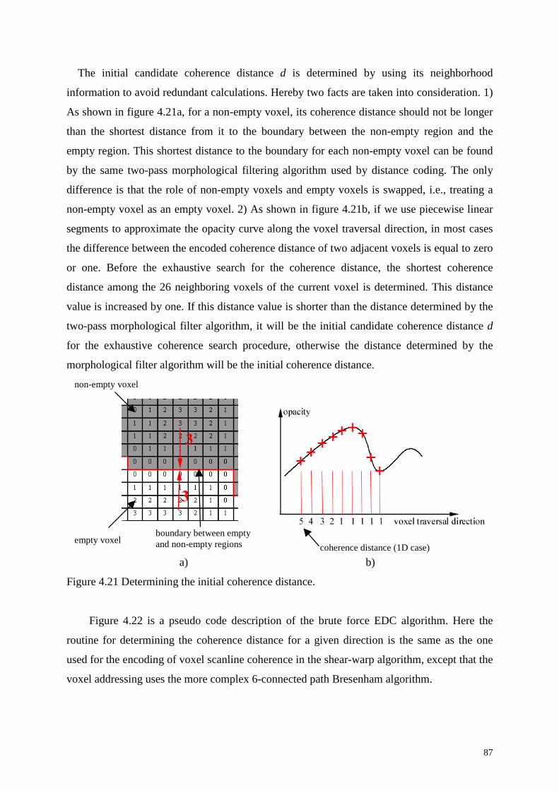
87

The initial candidate coherence distance d is determined by using its neighborhood

information to avoid redundant calculations. Hereby two facts are taken into consideration. 1)

As shown in figure 4.21a, for a non-empty voxel, its coherence distance should not be longer

than the shortest distance from it to the boundary between the non-empty region and the

empty region. This shortest distance to the boundary for each non-empty voxel can be found

by the same two-pass morphological filtering algorithm used by distance coding. The only

difference is that the role of non-empty voxels and empty voxels is swapped, i.e., treating a

non-empty voxel as an empty voxel. 2) As shown in figure 4.21b, if we use piecewise linear

segments to approximate the opacity curve along the voxel traversal direction, in most cases

the difference between the encoded coherence distance of two adjacent voxels is equal to zero

or one. Before the exhaustive search for the coherence distance, the shortest coherence

distance among the 26 neighboring voxels of the current voxel is determined. This distance

value is increased by one. If this distance value is shorter than the distance determined by the

two-pass morphological filter algorithm, it will be the initial candidate coherence distance d

for the exhaustive coherence search procedure, otherwise the distance determined by the

morphological filter algorithm will be the initial coherence distance.

a) b)

Figure 4.21 Determining the initial coherence distance.

Figure 4.22 is a pseudo code description of the brute force EDC algorithm. Here the

routine for determining the coherence distance for a given direction is the same as the one

used for the encoding of voxel scanline coherence in the shear-warp algorithm, except that the

voxel addressing uses the more complex 6-connected path Bresenham algorithm.

coherence distance (1D case)

non-empty voxel

empty voxelboundary between emptyand non-empty regions

88

procedure bruteForceEDC()

{

InitializeCoherenceDistanceWithMorphologicalFilter()

// assign each voxel an initial coherence distance which is its distance // to the nearest empty voxel in its neighborhood.

for z=0 to volumeSizeZ

for y=0 to volumeSizeY

for x=0 to volumeSizeX

{

if(opacity[z][y][x]!=0) //only non-empty voxel need process

{

candidateDistance=distance[z][y][x]&0x7F;

// get the distance and get rid of the flag bit.

expectedMaxDistance=smallestDistanceIn26Neighborhood(x,y,z)+1;

// exploit the fact that the difference between the coherence distances // of two adjacent voxels is equal to or less than one.

candidateDistance= expectedMaxDistance>candidateDistance?

candidateDistance:expectedMaxDistance;

do

{

candidateDistanceOk=true;

for each voxel (xb yb zb) on the box centered at (x,y,z) with edge of 2× candidateDistance

{

if ( errlinearization(x, y, z, xb, yb, zb)> = maxionlinearizaterr )

{

candidateDistanceOk=false;

candidateDistance--;

break; // start the check for the decreased distance at once

}

}

} while (candidateDistanceOk!=true && candidateDistance>1 )

distance[z][y][x]=candidateDistance+0x80; //add a flag bit and save the distance

}

}

}

Figure 4.22 The pseudo codes for the brute force EDC algorithm (continued)

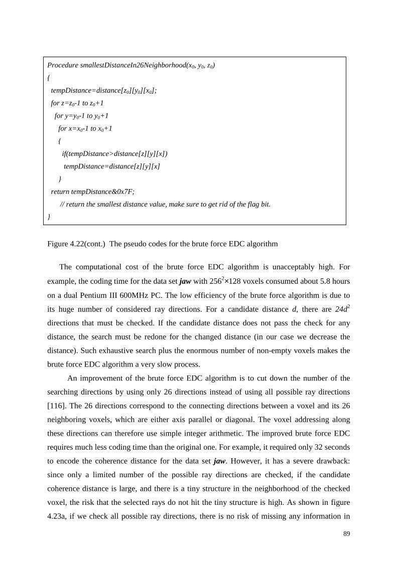
89

Procedure smallestDistanceIn26Neighborhood(x0, y0, z0)

{

tempDistance=distance[z0][y0][x0];

for z=z0-1 to z0+1

for y=y0-1 to y0+1

for x=x0-1 to x0+1

{

if(tempDistance>distance[z][y][x])

tempDistance=distance[z][y][x]

}

return tempDistance&0x7F;

// return the smallest distance value, make sure to get rid of the flag bit.

}

Figure 4.22(cont.) The pseudo codes for the brute force EDC algorithm

The computational cost of the brute force EDC algorithm is unacceptably high. For

example, the coding time for the data set jaw with 2562×128 voxels consumed about 5.8 hours

on a dual Pentium III 600MHz PC. The low efficiency of the brute force algorithm is due to

its huge number of considered ray directions. For a candidate distance d, there are 24d2

directions that must be checked. If the candidate distance does not pass the check for any

distance, the search must be redone for the changed distance (in our case we decrease the

distance). Such exhaustive search plus the enormous number of non-empty voxels makes the

brute force EDC algorithm a very slow process.

An improvement of the brute force EDC algorithm is to cut down the number of the

searching directions by using only 26 directions instead of using all possible ray directions

[116]. The 26 directions correspond to the connecting directions between a voxel and its 26

neighboring voxels, which are either axis parallel or diagonal. The voxel addressing along

these directions can therefore use simple integer arithmetic. The improved brute force EDC

requires much less coding time than the original one. For example, it required only 32 seconds

to encode the coherence distance for the data set jaw. However, it has a severe drawback:

since only a limited number of the possible ray directions are checked, if the candidate

coherence distance is large, and there is a tiny structure in the neighborhood of the checked

voxel, the risk that the selected rays do not hit the tiny structure is high. As shown in figure

4.23a, if we check all possible ray directions, there is no risk of missing any information in

90

the neighborhood of the considered voxel; if less viewing directions are examined, as shown

by figure 4.23b, the risk of missing information increases with the encoded coherence

distance. Thus the tiny structure might be lost in the images rendered with some settings of

the viewing matrix.

a) Check all possible ray directions b) Check a subset of possible ray directions

Figure 4.23 Drawback of examining less viewing directions (2D case). a) By checking allpossible ray directions, there is no risk of missing any tiny structures in the neighborhood. b)If only a subset of the possible ray directions are checked, the possibility of missing tinystructures increases with the coherence distance length. For the selected ray directions in thisfigure, with the distance being equal to or less than 4 there is no risk of missing information;with the distance being 5, there are eight directions (defined by the eight voxels which are notchecked) that may cause error; with the distance being 6, the directions that may lead to imageerrors or the missing of tiny structures is even more.

The brute force EDC algorithm consumes too much encoding time, therefore it can not be

used in practice. On the other hand, although the improvement of the brute force EDC

algorithm by considering less view directions can save a lot of the coding time, the image

quality can not be guaranteed. These drawbacks of the brute force EDC algorithm make us

turn to a more reliable approach.

4.4.3 The Taylor-Expansion-based EDC

The kernel idea behind the EDC is to assign a view-independent maximal spatial

coherence distance to each voxel in the volume, so that along any ray direction, the

integration of the difference between the actual opacity curve and a straight line taken to its

absolute value is less than an error bound ε, e.g.

distance = 4

distance = 5

distance= 6

voxel hit by theselected raysvoxel not hit by

the selected rays

91

})0(,)0()(

,1,

,)()(max{

3

0

fbandl

fLlfaLRL

dxbaxLxfRldl

=−==∈∀

≤+−∈= ∫+

ε 4.7∗

In the brute force EDC, for each candidate coherence distance, the integration of the error

is evaluated for each ray direction. If in any direction the error is larger than the error bound,

the procedure must be repeated by decreasing the candidate distance value. Moreover, when

the candidate distance is changed, most directions that are checked do not coincide with the

directions that have been checked (figure 4.24), therefore the error integration must be

calculated completely again for most directions. Thus the brute force EDC can not be

accelerated by reusing the intermediate calculation results.

Figure 4.24 The selected ray directions for different candidate coherence distances.

In order to decrease the preprocessing time for the EDC, we need to consider alternative

approaches. The EDC is nothing more than an approach to describe objects (coherence

regions) in a volume. According to [117], objects are only known through measures in forms

of test sets. Measure used in 4.7 is the error integration which is dependent on both the

considered direction and the size of the linear domain. In order to make the coherence

distance view-independent, any possible combination of the view-direction and the coherence

distance is checked to guarantee that the measure meets certain conditions (here the condition

is that the error is less than the pre-defined error bound). If proper measures in other forms

which are independent of the view directions can be used to describe the EDC, we may be

able to avoid the exhaustive combination checking of view-directions and coherence distance

and find more efficient EDC approaches.

One method is to use the traditional match-filter. The encoded coherence distance of a

voxel defines a patch of a hyper-plane which approximates the opacity function in its

∗ For convenience, a local coordinate system is used by taking the considered voxel as the origin.

92

neighborhood. The hyper-plane patch is described by its normal vector and its dimension

(coherence distance). From the point of view of the traditional signal processing, the EDC can

be implemented by convoluting a set of predefined templates (hyper-plane patches that have

different normal vectors n�

and dimensions l) with the opacity function of the volume and

finding the template whose size is the largest among all well matched templates (in terms of

similarity measured by the correlation coefficient). With this method the coherence distance is

given by

},)(*)(

)(*)(max{)( 3

,,

, RnthxTxT

xTxfRlxd

lnln

ln ∈∀≥∈= + �

��

��

�

. 4.8∗

In 4.8 th is the user-defined threshold for the similarity. The measure is now the similarity

between the templates and the coherence region in the volume.

Similarly, the EDC may be implemented by using morphological signal processing. Leo

Dorst [118] has shown that the morphological signal processing has computational structures

analogical to the traditional signal processing. For example, under the so called slope domain,

the dilation becomes addition (this is analogical to the fact in traditional signal processing that

the convolution in time or space domain becomes multiplication in frequency domain). This

indicates that we may design a morphological match filter to encode the coherence distance

just like using a traditional match filter. The basic morphological transformations are erosion

and dilation. These transformations involve the interaction between an object to be processed

and a structuring element. Like the above traditional signal processing based approach,

multiple structuring elements should be used for the EDC. Each structure element represents a

corresponding form of coherence region in the volume.

In such approaches the measures are not directly connected with the view directions any

more. However, this does not necessarily mean the derived coherence distance encoding

algorithms will be more efficient than the brute force EDC. In the match filter approach, the

measure is based on the normal vector n�

and the dimension l of the templates (hyper-plane

patches). The number of combinations of the normal vector and the dimension is the same as

that of the combinations of the view direction and the coherence distance, since the view

direction and the normal vector are both three dimensional variables. The discrete slope

∗ Instead of using the self-correlation of the volume opacity function, the self-correlation of the template is usedto normalize the correlation function between the template and the volume, since here the template is dynamicaland the best template is the object to be searched.

93

transform [118], which is to the morphological signal processing what the Fourier transform

is to linear signal processing, is still not well studied. The high dimensional form of the slope

transform is unknown. In addition, the slope transform requires that the functions are convex.

This is not true for the 3-D density function of volumetric objects. Hence the slope transform

theorem needs to be further developed to be applicable to the spatial coherence encoding of

volume objects.

The brute force EDC can be simplified by applying the Taylor expansion. Without loss of

generality, we first consider the linearization of a 1-D function f(x).

In 4.7 the parameter a can be approximated by the local gradient. The local gradient is

given by the first-order differential value of the function. According to the Taylor formula, if

the function is second-order differentiable, in the neighborhood of the point x=0, the function

f(x) can be represented by a linear function

)()0()0()( xRfxfxf +′⋅+= 4.9

with the remainder

],0[)(2

)(2

xfx

xR ∈′′= ξξ . 4.10

Approximate the parameter a in 4.7 by )0(f ′ , we have

)(2

))0()0(()()()(

2

ξfx

ffxLxfbaxLxf

′′=

+′⋅−=+−��

4.11

There exists a xmax in the neighborhood [0, x] so that the following condition always holds,

)()(],,0[, maxmax xffxx ′′≤′′∈∀∃ ξξ 4.12

The coherence distance can therefore be calculated by

}dx)x(f2

xRlmax{d

l

0 max

2

ε≤′′∈= ∫+ 4.13

94

Unlike the brute force EDC, formula 4.13 allows us to calculate the coherence distance

without explicitly evaluating the parameter a for each possible ray direction as well as the

error integration. As analyzed previously, when the candidate distance in the brute force EDC

is changed, most directions that are checked do not coincide with the directions that have been

checked (figure 4.24), resulting in that the calculation results for the parameter a and the error

integration are not reusable for the changed candidate coherence distance. In 4.13, the

coherence distance is determined by the maximal second-order differential value, which does

not depend on the ray directions, but only on the size of the coherent region, leading to much

more simple implementation of the coding process than the brute force EDC. Moreover, the

intermediate calculation results, namely the second-order differential values, are reusable,

since for a given function the second-order differential values are fixed and can be calculated

in advance.

Using 4.13 the coherence distance can be calculated as follows. First the upper bound

of the error for linearizing a function can be calculated by

)x(f6

ldx)x(f

2

xdx)x(R)l(error max

3l

0 max

2l

0′′=′′≤= ∫∫ . 4.14

For the given error bound maxionlinearizaterr , the coherence distance l yields,

maxmax

3

)(6

)( ionlinearizaterrxfl

lerror ≤′′≤ . 4.15

Thus the maximal coherence distance is given by

3)(

6

max

max

xf

err ionlinearizatl ′′≤ . 4.16

For 3-D functions we have

3)x(f)x(f)x(f)x(f)x(f)x(f

err6

maxyzmaxxzmaxxymaxzzmaxyymaxxx

maxionlinearizatl

������ ′′+′′+′′+′′+′′+′′≤ . 4.17

95

This means, the local coherence distance value of a voxel is determined by the allowed

error maxionlinearizaterr and the maximal second-order differential value (second-order difference

value for the discrete case) in the voxel neighborhood.

To efficiently find the local coherence distance, we use a two-pass encoding process. In

the first pass for each voxel position a distance value is determined by its local second-order

difference value and the error bound by using the following equation,

≠′′

≠′′=

′′

0),,(

0),,(

),,(

3),,(

6 max

zyxfDistancemaxAllowed

zyxf

zyxlzyxf

err ionlinearizat

4.18

where

),,(),,(),,(),,(),,(),,(),,( zyxfzyxfzyxfzyxfzyxfzyxfzyxf yzxzxyzzyyxx ′′+′′+′′+′′+′′+′′=′′ .

In the second pass the coherence distance for a voxel is calculated by either using an

iteration process or using a flood-fill algorithm. The former iteratively checks whether there

is any distance value in the temporary buffer smaller than the current candidate coherence

distance in the cubic neighborhood determined by the current candidate coherence distance. If

such distance value is found in the temporary distance buffer, the current coherence distance

is decreased by one, and the iteration is repeated in the downsized neighborhood. This

iteration procedure is much slower than the flood-fill approach. Therefore in practice the

flood-fill algorithm is adopted. The flood-fill process reads the distance value l of each voxel

determined by equation 4.18 from the temporary buffer and compares it with all the distance

values in the 3-D l-neighborhood of the voxel. All distance values which are larger than l are

updated by setting them to l. Otherwise the original value is kept.

The pseudo code for the Taylor expansion based EDC is shown in Figure 4.25. In the

pseudo code the flood-fill approach is used. This EDC method is quite fast and requires less

than 12 seconds for all data sets that we have tested (with up to 8M voxels).

96

procedure floodFillTaylorEDC(){

initializeCoherenceDistanceWithWavefrontAlgorithm()

// assign each non-empty voxel an initial coherence distance which is its distance

// to the nearest empty voxel in its neighborhood.

initializeTemporaryDistanceBuffer()

// calculate a distance for each voxel by using 4.18 and store it in the temporary distance buffer.

for z=0 to volumeSizeZ

for y=0 to volumeSizeY

for x=0 to volumeSizeX

if(opacity[z][y][x]!=0) //only non-empty voxel need process

{

l=temporaryDistanceBuffer[z][y][x];

for cubeZ=z-l to z+l

for cubeY=y-l to y+l

for cubeX=x-l to x+l

{ // check all distance values in the distance array inside the 3D l-neighborhood

// of (x,y,z) and let l replace the values larger than l.

if(l<distance[cubeZ][cubeY][cubeX]&0x7F)

distance[cubeZ][cubeY][cubeX]=l+0x80;

// decrease the distance value to l and set the flag bit

}

}

}

Figure 4.25 The pseudo codes for the Taylor expansion based EDC algorithm.

The Taylor expansion based EDC process can also be accelerated by using spatial

hierarchical data structures like pyramid data structures. Figure 4.26 shows the pyramid

hierarchy in 1D case. In this hierarchy, the nodes in the higher level contain the minimum of

their descendants. When checking the coherence distance value of a voxel, if the value of a

node in the neighborhood is larger than the coherence distance of the considered voxel, we

need not bother to check the whole branch whose root is the node, since it contains the

minimum of the whole branch. In this way, we can efficiently determine whether there is any

distance value less than the candidate coherence distance in the neighborhood of the

considered voxel without exhaustively checking each voxel.

97

Figure 4.26 Pyramid hierarchical data structure in 1D case.

The encoding process using the pyramid data structures consists of the following steps:

1) After each voxel is assigned a distance by applying (4.15), create a pyramid. Each

node at a certain level of the pyramid contains the shorter distance of its two direct

descendants (in 3D case there are eight direct descendants for each node on a higher

level). For example, the distance for node f at the pyramid level 1 in figure 4.26 is 9,

the shorter one of its two descendants V1 and V2; the distance for node d at the

pyramid level 2 is 5, the shorter one of its two descendants f and g, and so on.

2) For each voxel in the volume, find the maximal possible coherence distance by using

the pyramid data structure. This step has several substeps as following.

a) Read the distance value d of the current voxel from the distance buffer.

b) Calculate the most proper pyramid level l which matches the current candidate

distance by using formula l=(int)ceil(log2d).

c) Determine the node coordinate c of the current voxel in the pyramid level l.

d) Check the distance values of the node c and its adjacent siblings. If there is any

sibling whose distance value is less than the distance value d, traverse the sibling

and check whether in the sibling any distance value locating in the d-neighborhood

of the current voxel is less than d. If such a distance value exists, decrease d by one

and start a recursive procedure till the updated distance d is ok.

e) Store the distance value d as the final coherence distance in the distance array;

The spatial hierarchical data structures accelerated EDC has not yet been implemented in the

current ray casting program.

98

4.5 Implementation of the Accelerated Ray-castingAlgorithm In our new ray casting program the coherence acceleration is combined with the other

two acceleration techniques, i.e. early ray termination and space leaping.

Figure 4.27 is the kernel of the new ray casting algorithm, namely the procedure for the

processing of a single ray which originates from the virtual viewer and penetrates into the

volume generating a pixel on the image plane.

The input data of the procedure are a ray pointer aRay and a boolean variable

useNewMethod. The data structure ray has a scalar element distanceToGo, a scalar element

transparency, a vector element color, a direction vector dir, and a position vector pos. If a ray

is initialized, its pos element is set to the viewer position; its direction vector dir points from

the viewer to the current pixel on the image plane; all components of the color vector are set

to zero, and the transparency is set to one; its distanceToGo is set to the distance from the

viewer to the far clip-plane. The boolean variable useNewMethod is used to turn on or turn off

the coherence acceleration, so that we can examine the contribution of the coherence

acceleration to the performance improvement of the ray casting program.

The ray casting program is written in C++ under Linux. Except for Qt [119], it does

not rely on any other special library, therefore our ray casting program can be easily ported to

other platforms like Windows NT etc. Qt is a cross-platform C++ GUI application

framework. It provides programmers with all the functionality needed to build state-of-the-art

graphical user interfaces. We use Qt to simplify the programming of the user interface. As we

discussed in chapter 2, it is often necessary for a user to interactively change the visualization

parameters during the visualization process. With the support of Qt, our program is equipped

with an efficient interface to control the behavior of the ray casting. The structure overview of

the ray casting program is presented in Appendix B.

99

procedure algorithmicOptimizedRayCasting( ray * aRay, bool useNewMethod){ vector point1, point2; float spec1, diff1, spec2, diff2; // varaibles for specular and diffuse reflections. float opacity1, opacity2; // opacity at the sample point. if( rayVolumeBoundingboxIntersection( aRay, point1, point2) ) // check to see if the ray intersect with the volume, the ray need process // only if it intersects the volume. { aRay->distanceToGo=distance(point1,point2); //only the segment of the ray within the volume need process aRay->pos=point1; // move the current position of the ray directly to the first ray-volume intersection point . sampleBuffered = false; // for avoiding redundant resampling. if(useNewMethod) // early-ray-termination + space-eaping + coherence acceleration while( aRay->distanceToGo>0 && aRay->opacity > earlyRayTerminationThreshold ) { distance=getDistance(aRay->pos); if(distane&0x80) // it is a non-empty voxel { distance=distance&0x7F; // get rid of the flag bit. aRay->distanceToGo-=distance; if( sampleBuffered ) // last ray segment is also non-empty, { // no need to sample the first point. opacity1= opacity2; diff1=diff2; spe1=spe2; } else { volumeResamplingAndNormalEstimation(aRay->pos, &opacity1, &normal); calculateShading(normal, spec1,diff1); //evaluate the shading and opacity for the first sample point } moveRayForword(aRay, distance); volumeResamplingAndNormalEstimation(aRay->pos, &opacity2, &normal); calculateShading(normal, spec2,diff2); sampleBuffered = true; // let sampled info available for next coherent segment. diff1=(diff1+diff2)/2; spe1=(spe1+spe2)/2; //average the shading to avoid noise tmpOp=opacity1; opacity1=(opacity2-opacity1)/distance; for(i=0;i<distance;i++) // compositing the ray segments { aRay->color.r+=(tmpOp*(spec1+(diff1+amb)*colors[tmpOp].r)) * light.r *aRay-> transparency; aRay->color.g+=(tmpOp*(spec1+(diff1+amb)*colors[tmpOp].g)) *light.g *aRay-> transparency; aRay->color.b+=(tmpOp*(spec1+(diff1+amb)*colors[tmpOp].b)) *light.b *aRay-> transparency; aRay->transparency*=(1-tmpOp); tmpOp+=opacity1; } }

Figure 4.27 The kernel pseudo code of the new ray casting algorithm (continued).

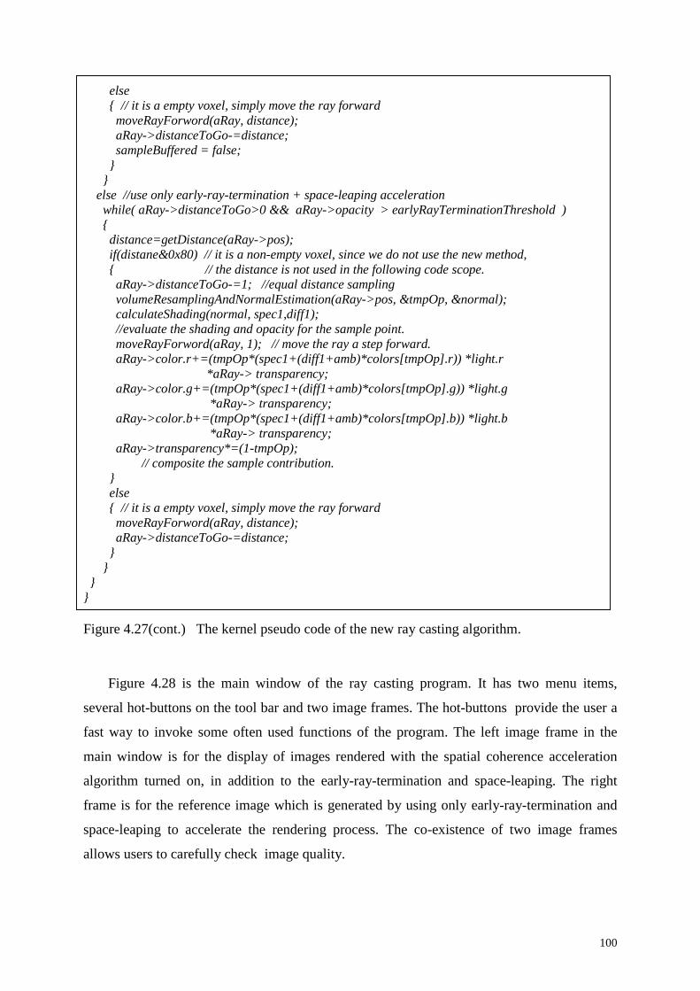
100

else { // it is a empty voxel, simply move the ray forward moveRayForword(aRay, distance); aRay->distanceToGo-=distance; sampleBuffered = false; } } else //use only early-ray-termination + space-leaping acceleration while( aRay->distanceToGo>0 && aRay->opacity > earlyRayTerminationThreshold ) { distance=getDistance(aRay->pos); if(distane&0x80) // it is a non-empty voxel, since we do not use the new method, { // the distance is not used in the following code scope. aRay->distanceToGo-=1; //equal distance sampling volumeResamplingAndNormalEstimation(aRay->pos, &tmpOp, &normal); calculateShading(normal, spec1,diff1); //evaluate the shading and opacity for the sample point. moveRayForword(aRay, 1); // move the ray a step forward. aRay->color.r+=(tmpOp*(spec1+(diff1+amb)*colors[tmpOp].r)) *light.r *aRay-> transparency; aRay->color.g+=(tmpOp*(spec1+(diff1+amb)*colors[tmpOp].g)) *light.g *aRay-> transparency; aRay->color.b+=(tmpOp*(spec1+(diff1+amb)*colors[tmpOp].b)) *light.b *aRay-> transparency; aRay->transparency*=(1-tmpOp); // composite the sample contribution. } else { // it is a empty voxel, simply move the ray forward moveRayForword(aRay, distance); aRay->distanceToGo-=distance; } } }}

Figure 4.27(cont.) The kernel pseudo code of the new ray casting algorithm.

Figure 4.28 is the main window of the ray casting program. It has two menu items,

several hot-buttons on the tool bar and two image frames. The hot-buttons provide the user a

fast way to invoke some often used functions of the program. The left image frame in the

main window is for the display of images rendered with the spatial coherence acceleration

algorithm turned on, in addition to the early-ray-termination and space-leaping. The right

frame is for the reference image which is generated by using only early-ray-termination and

space-leaping to accelerate the rendering process. The co-existence of two image frames

allows users to carefully check image quality.

101

Figure 4.28 The main window of the ray casting program.

The behavior of the ray casting program is controlled by a modeless dialog pad as shown

in figure 4.29. It has three tabs: a volume tab, a scene tab and a color tab. In the volume tab,

the user can assign or change the volume classification parameters, the error bound for the

EDC, and the material properties like the specular and diffuse reflection coefficient etc. In the

scene tab, the user can interactively change the viewing matrix as well as the illumination

condition by moving the location of a point-light source in the space. The last tab is used to

define the light color, background color, and colors of opaque voxels and semi-transparent

voxels.

If the user has changed any visualization parameters, he can see the result in the image

frames by simply clicking the camera icon on the tool bar. Except showing the images on the

screen, the program can also save the rendered images and other statistic results like the

preprocessing time, rendering time etc. in several different data files for later analyses.

102

Figure 4.29 The dialog pads for interactive control of visualization parameters.

4.6 Results and Analyses

We experimented the EDC based ray casting algorithm and compared the performance

of the new algorithm with that of the reference rendering scheme which uses only early-ray-

termination and space-leaping. All experiments were carried out by using half of the voxel

size as the sample unit to avoid artifacts as suggested by [43]. In the experiments different

opacity transfer functions were tested in order to find what kind of volume classification is

best accelerated by our method. The size of the output images is 256×256.

For convenience we call the EDC based ray casting the new method, and the reference

ray casting scheme which uses only early-ray-termination and space-leaping is called the old

method.

To compare the performance we use two metrics — rendering time and sample number.

Two speedup factors, namely speedup-I and speedup-II, are derived from these two metrics.

Speedup-I is the rendering time ratio between the old method and the new method. Speedup-II

is the ratio of sample numbers between the old method and the new method. The rendering

time depends on the used computer platform. The same program may take quite different time

to render the same scene on different computer systems, since the actual computing power is

determined by many factors, such as the cycle per instruction (CPI) of the CPU, the CPU

clock rate, the memory bus bandwidth, and the cache size etc. In addition, the optimization of

the program also affects the rendering time. Therefore, the rendering time and speedup-I are

not cross-platform fairly comparable. Nevertheless, we include the rendering time and

speedup-I in the experimental results to show the performance of the ray casting algorithm on

103

the computer system which we used to test the new algorithm. On the other hand, the sample

number is a metric which does not change with the performance of the computer platform and

the software. It shows the performance improvement accurately. From now on if we talk

about the speedup without specification, we imply Speedup-II, which is based on the sample

number and is cross-platform compatible.

Table 4.2 and table 4.3 contain the experimental results for two coherence encoding

approaches, i.e. the brute force EDC and the Taylor expansion based EDC. The results are

obtained by using the opacity transfer functions that make a large portion of the volumes

semi-transparent.

The encoding times listed in table 4.2 show that the brute force EDC is intolerably slow.

For most of the typical data sets the preprocessing varies between five minutes and several

hours, showing the strong dependence on the data set features, hence it is worthless in real

applications. The Taylor expansion based EDC is fast. For all data sets the preprocessing time

is less than 12 seconds (on a PC with 450 MHz Pentium III CPU with 512MB RAM).

Moreover, the encoding time is not as sensitive to the data feature as the brute force EDC.

Under the same allowed encoding error, the resulting image error for the Taylor

expansion based EDC is noticeably lower than the brute force EDC, this may be due to the

fact that the coherence distance is under-estimated by over-estimating the remainder of the

Taylor expansion, therefore in the Taylor expansion based EDC the error of approximating

the opacity curve with linear segments is less than the brute force EDC which calculates the

error exactly. Indeed, as the columns for the average coherence distance in table 4.2 and 4.3

show, for the same data set, the average coherence distance encoded by using the Taylor-

expansion based EDC is shorter than the distance encoded by the brute force EDC. The

under-estimation of the coherence distance for the given error bound in the Taylor expansion

based EDC thus makes its speedup lower than the speedup achieved when the brute force

EDC is used.

The main drawbacks of the Taylor expansion based EDC is that it needs an auxiliary

distance buffer to save the local coherence distance which is of the same size as the volume

data. But nowadays, as huge and cheap memory devices are becoming widely available,

desktop PCs with 512MB~1GB RAM are very common, so the extra memory requirement is

not a problem. By default, our ray-casting program uses the Taylor expansion based EDC,

because on the one hand the Taylor expansion based EDC reduces the preprocessing time of

the brute force EDC by a factor of two or three orders of magnitude, making the

preprocessing an acceptable procedure; and on the other hand, the performance loss (speedup

104

decrease) caused by the under-estimation of the coherence distance by the Taylor expansion

based EDC is not severe. In the following analyses we use the experimental results which are

generated by using the Taylor Expansion based EDC.

Rendering time(seconds)

Sample number

Data setEncoding

time(seconds)

Averagecoherencedistance

Imageerror(%) Old

methodNew

method

Speedup-IOld

methodNew

method

Speedup-II

MRI Brain(1282×84)

700.01 2.16 3.44% 5.16 3.31 1.56 1589334 771711 2.06

Head(2562×113)

3746.80 3.01 3.05% 5.01 3.28 1.53 1422045 714595 1.99

Engine1(2562×110)

318.17 2.19 3.63% 7.97 4.95 1.61 1980934 971058 2.04

Engine2(2562×110)

398.00 2.41 3.18% 8.63 4.89 1.76 2124533 945371 2.25

Jaw(2562×128)

21037.09 5.03 6.28% 15.1 5.97 2.53 3952777 1170846 3.38

Jaw(2562×128,inner view)

(21037.09) (5.03) 12.76% 36.12 9.26 3.90 9540125 1743443 5.47

Heart (202×132×144)

2053.89 4.13 7.44% 8.64 3.30 2.61 2277821 742484 3.07

Table 4.2 The performance of the spatial coherence accelerated ray casting by using the bruteforce EDC. Larger portion of the volumes are mapped semi-transparent.

Rendering time(seconds)

Sample number

Data setEncoding

time(seconds)

Averagecoherencedistance

Imageerror(%) Old

methodNew

method

Speedup-IOld

methodNew

method

Speedup-II

MRI Brain(1282×84)

1.19 1.98 1.32% 5.16 3.36 1.54 1589334 805950 1.97

Head(2562×113)

7.03 2.08 1.45% 5.01 3.31 1.51 1422045 747658 1.90

Engine1(2562×110)

5.64 2.04 1.83% 7.97 5.31 1.50 1980934 1020521 1.94

Engine2(2562×110)

5.46 2.23 0.74% 8.63 5.29 1.63 2124533 979264 2.17

Jaw(2562×128)

11.65 3.06 2.31% 15.1 6.59 2.29 3952777 1380111 2.86

Jaw(2562×128,inner view)

(11.65) (3.06) 10.39% 36.12 13.32 2.71 9540125 2731994 3.49

Heart (202×132×144)

2.81 2.69 3.52% 8.64 4.27 2.02 2277821 901037 2.53

Table 4.3 The performance of the spatial coherence accelerated ray casting by using theTaylor expansion based EDC. The visualization parameters are the same as in table 4.2.

The achieved speedup is dependent on the features of the data sets. As shown in table

4.3, the speedup ranges between 1.90 and 3.49 (in terms of the sample number ratio).

The higher speedups are obtained with the data sets Jaw and Heart. The highest

speedup, 3.49, is about 1.84 times larger than the lowest speedup obtained with the data set

Head. The reason for this is that in different volume data sets the portion of volume inside

which high coherence is available is quite different. In Jaw and Heart, the semi-transparently

mapped soft tissue occupies considerably large regions. In such regions coherence exists,

therefore the coherence acceleration can fully perform. On the contrary, in the volume head,

105

the soft (semi-transparent) tissue between the empty space (the air) and the opaque skull is

thin. In that case the combination of early-ray-termination and space-leaping is efficient,

while only a marginal speedup can be obtained by the coherence acceleration. In more

extreme cases, i.e. if the voxels in the volume are classified so that most of them are either

transparent or opaque, the contribution of the coherence acceleration will become negligible,

since space-leaping and early-ray-termination leave no space for coherence acceleration to

play its role. Table 4.4 shows such results for the empty-opaquely mapped data sets. As we

see in this table, if the volume contains mainly opaque and empty voxels, the spatial

coherence accelerated algorithm presents almost no acceleration compared to the one

accelerated only with early-ray-termination and space-leaping. The reason is that a ray needs

only a few voxels to meet the condition of early ray termination after it has traversed through

the empty space in the volume. Thus the adaptive sampling in the non-empty regions of the

volume is unimportant, although, as shown in table 4.4, the average encoded distance for non-

empty voxels is not evidently shorter than that in table 4.3. However, such an extreme case of

volume classification is not practical. Instead, in many cases, the volume is usually classified

so that some parts of its structures are semi-transparent, while the other parts are either empty

or opaque, allowing different structures in the volume data to be visualized simultaneously.

Rendering time(seconds)

Sample number

Data setEncoding

time(seconds)

Averagecoherencedistance

Imageerror(%) Old

methodNew

method

Speedup-IOld

methodNew

method

Speedup-II

MRI Brain(1282×84)

0.70 1.81 1.93% 0.83 0.83 1.00 174341 174263 1.00

Head(2562×113)

5.65 2.61 2.47% 1.78 1.79 0.99 350175 350181 1.00

Engine1(2562×110)

4.66 2.27 2.11% 1.29 1.29 1.00 249541 248005 1.01

Engine2(2562×110)

4.92 2.34 1.16% 1.31 1.32 0.99 258891 257744 1.00

Jaw(2562×128)

9.66 2.91 1.47% 1.41 1.41 1.00 291268 290727 1.00

Heart (202×132×144)

2.28 2.83 1.51% 0.65 0.65 1.00 127628 126939 1.01

Table 4.4 The experimental results for volume data whose voxels are mapped either empty oropaque.

Images a, b, e, and f in figure 4.30 are the images of the volume data Engine-2 and

Heart which are rendered with many voxels semi-transparently mapped. For comparison,

their empty-opaquely mapped counterparts are listed in image c, d, g and h of figure 4.30. The

images show that the semi-transparently mapped volumes allow more information inside the

volume to be rendered. Images for other data sets can be found in appendix A. These images

106

show that it is difficult to differ the images rendered by the new method from the ones

rendered by the old method.

Figure 4.30 Volumes rendered with different opacity transfer functions (continued).

a) b)

c) d)

107

Figure 4.30 (cont.) Volumes rendered with different opacity transfer functions. The images onthe left are rendered with the new algorithm, the images on the right are rendered with the oldalgorithm.

As mentioned above, the achieved speedup is dependent on the data features. The

influence of the inherent features of volume objects on the performance is reflected in the

average length of the encoded coherence distance. The longer the average coherence distance,

the less sampling operations will be required along a ray, resulting in higher acceleration rate.

As table 4.3 shows, for the data set jaw which has the longest average coherence distance, the

achieved acceleration rate is the highest among all the data sets.

The noise in the volume is an important factor that shortens the adaptive sampling

interval and the average encoded coherence distance of non-empty voxels. The impact of

noise on the coherence distance is demonstrated by figure 4.31. In the left graph, to calculate

the ray integration with a given error, one needs only a few sample points with average longer

sampling intervals. However, when voxels are contaminated by noise, in order to approximate

e) f)

g h)

108

the ray integration with the same error, much more sample points that have shorter intervals in

between are necessary. During the EDC process, if there is strong noise in the neighborhood

of a voxel, a shorter coherence distance will be encoded in the distance array. If such a case

occurs frequently in a volume, the average encoded distance of non-empty voxels will

evidently decrease. Therefore by suppressing the noise in a preprocessing stage we can

increase the average encoded distance of non-empty voxels and thus improve the performance

of the new algorithm. We produced the data set engine2 from volume data engine1 by using a

non-linear diffusion filter to suppress the noise in the volume. After suppressing the noise in

the volume, the average coherence distance increases from 2.04 to 2.23. Correspondingly the

acceleration rate increases from 1.94 to 2.17, namely an efficiency improvement of 12%.

Besides, the image quality is also improved by filtering the noise in the original data set, as

can be seen in figure 4.32.

Figure 4.31 The impact of noise on the performance. The position of the sample points ismarked by the crosses. The left figure shows the sample points required in the noise-freevolume. The right figure shows the required sample points with strong noise presented in thevolume. The strong noise leads to more sample points along the ray.

Figure 4.32 The effect of filtering the noise in volume data. a) the original volume (Engine1).b) the image rendered with the noise suppressed (Engine2).

109

We studied the image quality and the speedups with respect to the error threshold used

for the coherence encoding. We use the same image quality metric described in section 4.2.4.

Figure 4.33 shows for the semi-transparently mapped data set Jaw how the average coherence

distance, the achieved speedup factor, and the image error change with respect to the

encoding error. The curves in the figure indicate, that if we tolerate more encoding error, the

coherence distance and the achieved speedup factor increases, but the image quality degrades.

The results are reasonable. However, it is not possible for us to predict the image quality by

the encoding error threshold, since on the one hand, in the volume compositing procedure the

ray intensity attenuation is defined by an exponential absorption function which is related to

the integral of the local absorption coefficient (refer to formulas 2.17 to 2.18 in chapter 2); on

the other hand, the error is distributed all the way along a ray, we do not know its exact

distribution in space (it is data-dependent), thus the error cannot be estimated in an analytic

way.

a) Coherence distance vs. encoding error b) Speedup vs. encoding error b) Image error vs. encoding error

Figure 4.33 The impact of the encoding error to the performance of the new algorithm. Thetested data is Jaw with the viewer located inside the volume.

Figure 4.33b shows that there is a non-linear dependency of the performance on the

encoding error so that larger tolerated encoding errors contribute less to the overall

performance improvement (in terms of the sample number based speedup-II) until it reaches a

plateau. To further increase the encoding error will result in an unacceptable image quality

while the performance improvement of the new method is very limited. Experimental results

show that the reasonable encoding error range is between 0.01 and 0.02 to achieve a balance

between the image quality and the acceleration rate.

0 0.005 0.01 0.015 0.02 0.0251

1.5

2

2.5

3

3.5

4

Spe

edup

-II

encoding error threshold0 0.005 0.01 0.015 0.02 0.025

0

2

4

6

8

10

12

14

Imag

e Er

ror

(%)

encoding error threshold0 0.005 0.01 0.015 0.02 0.025

1

1.5

2

2.5

3

3.5

aver

age

cohe

renc

e di

stan

ce

encoding error threshold

110

There is another factor that also affects the image quality, namely the distance of the

light source from the volume center. During the shading calculation we assume that within the

coherent ray segment the light direction vector is constant. This is approximately correct

when the light is located far enough from the volume, so that the direction from each voxel to

the light source can be considered parallel. But if the light is close to the volume, this will

lead to additional errors in the image. Figure 4.34 shows how the image error decreases as the

light source is more distant from the volume center. The error is normalized by the error of an

image rendered with a directional light source. As shown by the normalized error curve, when

the light is placed far enough from the volume, the error becomes identical to the error of the

image rendered with a directional light source and the constant shading assumption can

therefore be applied. Unlike in other application fields of computer graphics where the light

source position is dedicatedly selected to produce different special effects, in volume

rendering, the light is merely a method to give the image more visual hints instead of

producing special effects. Therefore we can arbitrarily place the light to any location which is

far away enough to make the constant shading assumption valid, or simply use a directional

light source.

Figure 4.34 Influence of light distance to the image quality.

The assumptions for simplifying the shading calculation are also made by the famous

volume rendering library VolPack. However, VolPack assumes not only fixed light direction,

but fixed viewing direction for the whole volume as well. Thus when the volume is rendered

with the viewer very close to the volume, the shading is not correct, especially the specular

reflection when the perspective projection is used. This is because in this case the actual

directions from the viewer to the voxels may differ strongly from each other. The incorrect

shading may make the rendered image very confusing and lead to misinterpretation of the

volume data. For our algorithm this problem does not exist, since the viewing direction is

111

identical to the ray casting direction. If only the light source is far away from the volume, our

method can calculate the shading correctly, even if the viewer observes the features in the

volume very closely, i.e. in the case of a data walk-through. In figure 4.35 one can observe

that some branches of the blood vessel on the heart surface are not visible in the image

rendered by VolPack due to incorrect shading, while they are perfectly rendered by our

program.

Figure 4.35 Shading comparison between the new algorithm and VolPack. The left imagewas rendered by our new algorithm. The right image was rendered with VolPack. Thehighlight rendered by VolPack is not realistic, and some vessels on the surface are not clearlyrendered as indicated by the red arrows.

4.7 Discussions By reducing the time-consuming tri-linear resampling and shading calculation in the

coherent regions of volumes, we successfully accelerated the ray casting process with a

speedup factor between 1.90 and 3.49 (in terms of sample numbers). The achievable

acceleration relies on the features of the data set as well as the opacity transfer function. Our

method has the best performance when the volume has a large portion of semi-transparent

regions for which the other acceleration techniques like early-ray-termination and space-

leaping are not efficient. For data sets with most of their voxels empty-opaquely mapped, our

method shows only marginal acceleration. For such data sets, however, early-ray-termination

and space-leaping can efficiently reduce the computational cost. Hence, by combining our

method with the early ray termination and space-leaping, we can achieve more stable frame

rate when different opacity transfer functions are used.

112

The coherence acceleration requires a preprocessing, i.e. EDC, to encode the local spatial

coherence information in a distance array. The brute force EDC is time consuming and

therefore not usable in practice. The Taylor expansion based EDC makes conservative under-

estimations of the coherence distance and achieves tremendous performance improvements in

terms of the required encoding time. For all data sets with up to 8M voxels ( 2562×128) the

encoding time is less than 12 seconds (the worst case is for the data set Jaw whose

preprocessing consumed 11.65 seconds). Such a preprocessing time can be considered

acceptable in practice. As we have seen in section 4.2.4, VolPack requires about 45 seconds

for the same data set. Besides, the encoding time may be further reduced by optimizations, for

example, using spatial data structures.

The image quality is affected by two factors: the shading error due to the assumption of

constant shading for the coherence region and the encoding error. The shading error decreases

as we increase the distance of the light source to the volume, thus we can simply use a

directional light source to make the light direction vector a constant for the whole volume.

Experimental results have shown that the image error increases with the encoding error, while

the acceleration rate gradually reaches a plateau. To guarantee the image quality, we usually

use an encoding error less than 0.02 in order to achieve a reasonable balance between the

acceleration rate and the image quality.

In addition, it is not difficult to implement our new ray casting scheme in volume

rendering oriented hardware, e.g. VGE, although small modifications are necessary as

discussed in the following.

By using a multi-threading based strategy, the VGE can fully support the acceleration

techniques like space-leaping and early-ray-termination [8]. Since space-leaping and our

coherence acceleration work in very similar way, both techniques read a distance value from

the distance array and use the distance value to determine the location of the next sample

point. Therefore, if the coherence acceleration is implemented in the VGE architecture, the

original voxel addressing and memory I/O control logic can be used without modification.

However, unlike space–leaping which does not carry out any operations to accumulate the

contribution of the empty voxels, the coherence acceleration needs operations to accumulate

the contribution of the coherent region by linearly interpolating the opacity at even-positioned

points within the linearized segment of the ray and updating the ray intensity with the so

called over operation. Since the coherence distance is adaptive, for a long coherence distance

more cycles of over operations are necessary. Therefore extra hardware resources may be

necessary to minimize the unbalanced computational burden caused by the adaptive

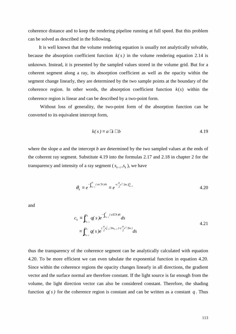
113

coherence distance and to keep the rendering pipeline running at full speed. But this problem

can be solved as described in the following.

It is well known that the volume rendering equation is usually not analytically solvable,

because the absorption coefficient function )s(k in the volume rendering equation 2.14 is

unknown. Instead, it is presented by the sampled values stored in the volume grid. But for a

coherent segment along a ray, its absorption coefficient as well as the opacity within the

segment change linearly, they are determined by the two sample points at the boundary of the

coherence region. In other words, the absorption coefficient function )(sk within the

coherence region is linear and can be described by a two-point form.

Without loss of generality, the two-point form of the absorption function can be

converted to its equivalent intercept form,

bsa)s(k +⋅= 4.19

where the slope a and the intercept b are determined by the two sampled values at the ends of

the coherent ray segment. Substitute 4.19 into the formulas 2.17 and 2.18 in chapter 2 for the

transparency and intensity of a ray segment ( k1k s,s − ), we have

ks

1ks2ks

1ks|)bss

2

a(ds)bas(

k ee −−+−+−

=∫=θ 4.20

and

dse)s(q

dse)s(qc

k

1k

21k

21k

k

1k

s

1ks

s

s

)bss2

a()bss

2

a(

s

s

dt)bta(

k

∫

∫

−

−−

−

−

+−+

+⋅−

=

∫= 4.21

thus the transparency of the coherence segment can be analytically calculated with equation

4.20. To be more efficient we can even tabulate the exponential function in equation 4.20.

Since within the coherence regions the opacity changes linearly in all directions, the gradient

vector and the surface normal are therefore constant. If the light source is far enough from the

volume, the light direction vector can also be considered constant. Therefore, the shading

function )s(q for the coherence region is constant and can be written as a constant q . Thus

114

we can move q and the constant component of the exponential function outside of the

integral formula,

dseqeck

1k

21k

21k s

s

)bss2

a()bss

2

a(

k ∫−

−− +−+⋅= 4.22

The integral in 4.22 is still not analytically solvable, but it can be solved by either applying

numerical integration like the Simpson rule or by expanding the exponential function into an

integrable polynomial. In this way the intensity contribution of a coherent segment can be

evaluated as a whole. Therefore the computational complexity of coherence acceleration is

not dependent on the length of the coherence distance and this will simplify the hardware

design.

The coherence acceleration algorithm may be extended by using higher order curves for

approximating the opacity curve along a ray, allowing longer coherence distance (figure

4.36). However, such extensions may not be as good as it seems to be. The reason is that the

longer coherence distance does not certainly lead to lower sampling rates. For a non-linear

curve, the number of sample points which are required to determine the curve segment is

proportional to the order of the curve. For a linear curve segment (it is one order) we need

only two sample points to definitely determine it; for a quadratic curve segment (a two order

curve) we need three sample points to determine it, and so on. On the other hand, it is

doubtful that the length of the encoded coherence distance will increase proportionally with

the order of the approximating curve. An alternative method for avoiding additional sample

points in the coherence region is to calculate and store the parameters for the curve segments

a) b)

Figure 4.36 Two strategies for opacity curve approximation. a) Using 10 short linesegments to approximate the curve. b) Using only 4 second order curve segments toapproximate the same curve.

115

approximating the original opacity curve during the preprocessing stage. The memory space

required to store the curve parameters, however, will be too large due to the number of

parameters. In addition, if high order curves are used to approximate the opacity curve, the

constant normal assumption within the coherence region is not valid any more. We can

therefore only use gradientless shading as we do in the new shear-warp algorithm, or use the

Gouraud shading which directly interpolates the intensity between sample points instead of

calculating the normal at each sample point and then calculating the shading. This leads to

either the lack of diffuse and specular lighting or to unrealistic highlighting. Consequently we

believe that it is worthless to achieve longer coherence distance by using high order curves for

approximating the opacity curve.

4.8 Chapter Summary

Exploiting coherence is one of the most commonly used approaches to accelerate volume

rendering. In this chapter we discussed the coherence acceleration for two volume rendering

algorithms, namely the shear-warp algorithm and ray casting.

For the shear-warp algorithm, the spatial coherence is encoded along the voxel scanline,

since the volume is exactly traversed in voxel scanline order. The coherence distances are the

lengths of linear voxel scanline segments which approximate the original opacity curve along

the voxel scanline with error less than a pre-defined error bound. During the rendering

process, each linear segment is reconstructed by using only the information of two voxels at

the ends of the linear segment, hence the sampling rate in the coherence regions is decreased.

The achieved speedup by the coherence acceleration, however, is marginal. In the best case

the speedup factor is only 1.29 (in terms of rendering time) compared to VolPack. One reason

for such results is that the reconstruction of the voxel values within the coherent segment

along the voxel scanline is not considerably cheaper than the direct voxel read-out from the

voxel array due to the high memory coherence of the shear-warp algorithm and the cheap

sampling kernel used in the shear-warp algorithm. In addition, the perpendicularity of the

voxel scanline traversal direction to the volume composition direction leads to the hiding of

achievable speedup by early-ray-termination.

For the ray casting algorithm, the spatial coherence in the volumes is view-independently

encoded and stored in a distance array at a preprocessing stage. This preprocessing stage is

called EDC (extended distance coding). During the ray casting process at each sample point in

116

the non-empty region of the volume the corresponding coherence distance is read out from the

distance array, and is used to determine the position of the next sample point along the ray. In

this way, we decrease the sampling rate in the coherence region by sampling only two

boundary points instead of equal-distantly sampling the volume along the ray.

The brute force EDC searches the most optimal coherence distance for each voxel by

checking all possible ray directions to guarantee that the coherence distance is view-

independent. The huge number of voxels in the volume and the huge number of the possible

ray directions make the brute force EDC intolerably slow. By constructing a relation between

the error bound of the EDC and the remainder of the Taylor expansion, we convert the

exhaustive view-dependent recursive search of the coherence distance to the search of the

local maximum of the second order partial difference of opacity value, leading to an efficient

Taylor expansion based EDC. While the required preprocessing time of the brute force EDC

ranges between about 5 minutes and several hours for volumes with 8 millions voxels, the

Taylor expansion based EDC needs less than 12 seconds for the same data sets.

The decrease of sampling rates through the utilization of the spatial coherence can

efficiently accelerate the ray casting process, the reasons are: 1) unlike in the shear-warp

algorithm, in the ray casting algorithm the volume is resampled by using the more expensive

tri-linear interpolation; 2) in the ray casting algorithm the volume is not traversed in storage

order, memory coherence is not as high as in the shear-warp algorithm, the decrease of

sampling rate helps to reduce the requirement on the memory bandwidth; 3) in the coherence

region the gradient is constant, the computationally expensive operations for calculating the

shading function can be reduced by evaluating the shading function only once for each

coherence region. We accelerated the rendering of semi-transparently mapped volumes with

speedup factor up to 3.49 (in terms of sample numbers). Thus we achieved our goal—

improving the ray casting of semi-transparently mapped volumes by a factor of about 2 or

even more.

Till now we considered only the volume rendering acceleration for a static volume object.

But in applications like surgical operation simulation, volume object are subject to

deformation. Fast rendering of the deformation of volumetric objects is very important in such

applications. From the next chapter on we begin with the other part of this dissertation – the

fast volume deformation algorithm.

117

Chapter 5

Object Deformation Techniques

Object deformation is a basic technique for modeling and animation. It is widely used in

applications like CAD/CAM, computer animation, virtual reality systems, e.g. surgical

simulation systems. For example, in the simulation of endoscopic procedures, object

deformation techniques are applied to blow up the area of investigation and deform the

oesophagus, the stomach, or the intestine as the endoscope is pushed through them.

In the simulation of volumetric object deformation, two principal problems are

considered. The first problem is how to describe the geometrical shape evolvement of the

deformable volume object. Like any other surface-based representation of objects, the shape

change of a volumetric object can also be determined by using traditional object deformation

methods, since from the geometrical point of view, the voxel (the elemental primitive of the

volume object) is the same as the vertices of a polygon model, both are 3-dimentional points

in space.

118

The second key problem in the simulation of volumetric object deformation is the

efficiency of the deformation process. The volume object is an exhaustive enumeration

representation of an object. Volume deformation by directly manipulating each voxel of a

volume object is therefore far from being real-time or interactive deformation rate. In order to

overcome this problem, volume deformation can be realized by e.g. 3D texture morphing

[120][121] and inverse-ray-deformation [59]. Such methods do not generate a deformed

volume object before rendering it. Instead, only the texture coordinates or the viewing rays

are deformed in the rendering process, thus the computations required by reconstructing a

deformed volume are saved.

In the following, we first discuss the approaches for describing object deformation,

namely the pure geometrically based deformation methods and the physically-based methods.

Then we discuss the previous work in volumetric object deformation and the drawbacks of the

existing approaches.

5.1 Geometric Deformation Methods The early work on object deformation was done by Alan Barr [59] at the beginning of

the 1980s. The deformation is described in terms of geometric mappings of three-dimensional

space. Mathematically, the geometric mappings can be represented by a transformation

function f: R3→R3, which explicitly modifies the global coordinates of points in three

dimensional space. Except for the simplest transformations like scaling and translation, in

most deformation procedures the object normal vectors are changed during the deformation

procedure. Allan Bar derived the normal vector transformation rule to calculate the surface

normal after the deformation. The normal vector transformation rule involves the transpose of

the inverse Jacobian matrix of the transformation function f and can be expressed as follows:

)p(n)J(Jdet)p(n T1 �� −⋅=′ . 5.1

where )p(n�

is the normal vector at the undeformed point p and )p(n ′�

is the normal vector at

the transformed position of the point p. The determinant of the Jacobian matrix is the local

volume ratio at each point in the deformation, between the deformed region and the

undeformed region, it can therefore be used to control the change of the object volume during

the deformation. Deformation methods which can preserve the object volume throughout the

deformation procedure can be found in [122, 123, 124]. In most surface-based computer

119

graphics applications, however, the determinant of the Jacobian matrix is not necessary to be

calculated, since the volume change is not considered, only the direction of the normal vector

is required to evaluate shadings. In volume deformation, as we will discuss in chapter 6, the

information of volume change is necessary for opacity compensation.

The deformation procedure developed by Barr is elegant due to the perfect analytic

expression of the deformation functions. For example, a global twist along the Z-axis can be

defined by the following function:

−=

z

y

x

zz

zz

p

p

p

100

0)pcos()psin(

0)psin()pcos(

)p(f 5.2

This function defines a twist which proceeds along the Z-axis at the rate of one radian per unit

length in the Z direction as shown in figure 5.1. The normal transformation matrix is given by

−

−=−

1

0)cos()sin(

0)sin()cos(

)( 1

xy

zz

zzT

pp

pp

pp

J 5.3

Figure 5.1 Global twist deformation ( From Maya©1 user guide).

1 Maya© is a professional 3D software of Alias|Wavefront, a division of Silicon Graphics.

120

Similarly, other deformation forms like tapering, bending etc. can be defined in the

same manner. More complicated deformations could be implemented by combining different

deformations in a hierarchical structure. This deformation method developed by Barr is a

powerful tool for object modeling and deformation and is still a standard tool in computer

graphics software. The drawback of this method is that there are only limited deformation

functions available and the deformations are regular. In addition, arbitrary deformation is

difficult, since the simulation of complicated deformations by combination of several

deformation procedures is not intuitive.

Morphing techniques are also used for object deformation [120, 125]. To generate a

smooth transition from the original object shape to its target shape, a pair of landmark point

sets is selected for both the original object and the target object. The landmarks are then used

to calculate the transformation of all points of the object. The morphing-based deformation is

however, not an “automatic” deformation method, since it relies on landmarks which must be

selected and positioned manually in advance.

Figure 5.2 Free-form-deformation (by NIBH [126]). a) A FFD grid and an object underdeformation. b) The deformed FFD grid and the deformed object.

A more versatile and intuitive approach for representing and modeling the object

deformation is free-form-deformation (FFD) [127]. The FFD is also a mapping from R3→R3.

Instead of using an explicit deformation function, the FFD defines the space mapping in terms

a) b)

W U

V

O

121

of a tensor product tri-variant Bernstein polynomial. The deformation procedure proceeds as

follows:

In the first step, the object subjected to the deformation is embedded in a parallelepiped

region of space. A local coordinate system is imposed on the parallelepiped region, as shown

in figure 5.2a. Any point P inside the region is specified by

wWvVuUOP +++= 5.4

The (u,v,w) coordinates of the point P in terms of the local coordinate system can be found by

the following calculation:

( ) ( )( )

( ) ( )( )

( ) ( )( ) WVU

OPVUw

VWU

OPWUv

UWV

OPWVu

⋅×−⋅×=

⋅×−⋅×=

⋅×−⋅×=

5.5

Note that for any point inside the parallelepiped region its coordinate values are between 0

and 1, i.e. 1w0,1v0,1uo <<<<<< .

In the second step, a grid of control points { k,j,igridP , 0<i<l, 0<j<m, 0<k<n} is imposed

on the parallelepiped region such that

Wn

kV

m

jU

l

iOP k,j,i

grid +++= 5.6

The deformation of the embedded object is specified by moving the control points

around from k,j,igridP to )P( k,j,i

grid ′ . After the control points have been moved to their new

position, any point of the object can be mapped to its new location by finding its local

coordinates (u,v,w) and then evaluating the tri-variant Bernstein polynomial:

( ) ( ) ( ) ( )∑∑∑= = =

′=′l

0in

m

0j

n

0kml

k,j,igrid w,kBv,jBu,iB)P(w,v,uP 5.7

122

One of many advantages of FFD is its general applicability to all representations of

embedded objects. In general, an object can be deformed by deforming all points that are

contained in the object. Nevertheless for most cases this is an impossible task. Usually only a

finite set of point is deformed. The deformed points are then used to reconstruct the deformed

object. For example, vertices of polygon meshes are directly mapped to their new position by

FFD, enabling planes to be moved and warped; Splines and spline patches are modified by

mapping their control points and derivatives. For an object represented by parametric or

implicit equations, the FFD defines a change of variables, thus the object remains parametric

or implicit after the deformation.

The FFD deformation is not necessarily formulated in terms of tensor product Bernstein

polynomials. Griessmair and Purgathofer [128] utilized a tri-variant B-Spline representation

for FFD. They suggested a set of criteria for the tessellation of a surface in order to minimize

the distortion in the deformation process. Since a polygon can be non-planar under

deformation, it must be approximated by many small polygons before the deformation takes

place in order to get an accurate model of the deformed surface. In our volume deformation

approach, we use the B-spline FFD, because B-splines have very good local properties and

allow implementation of deformation with cheaper calculation than the tensor product

Bernstein polynomials-based FFD. We will address this problem more detailed in section

6.2.1, where we will present the implementation of our deformation method.

5.2 Physically-based Object Deformation Physically-based deformation simulates the object behavior when it is subjected to

external forces by determining the deformation using physical laws. It makes the deformation

more realistic than the pure geometric-based deformation procedure. Physical models are

derived by applying the laws governing motion to the physical parameters of an object.

Typical physically-based object deformation models include: finite element method (FEM)

[129, 130, 131], mass-spring model [132, 133], particle system [134, 135] and, kinematic-

dynamic system ( e.g. Chainmail algorithms [136, 137]) etc. The literature on physically-

based deformation is very rich. In [138] Gibson has given a good survey of the deformation

methods. The physically-based deformation models and their application in the simulation of

soft tissue deformation can also be found in [139]. In the following, we summarize only three

commonly used techniques, the FEM, the mass-spring system, and the particle systems. The

summarization is mainly based on the work by Gibson [138], Zachow [139], and Szeliski

[135].

123

Among all physically-based deformation models the FEM is the most accurate one. It

considers the equilibrium of an object subjected to external forces. The deformation is defined

by the applied forces and the object’s physical properties. When the potential energy is at a

minimum, the object reaches its equilibrium state. The potential energy of the deformable

object is given by:

WEE sp −= 5.8

where sE is the strain energy of the deformable object which is stored in the object in form of

material deformation; W is the work done by the external forces.

If the derivation of pE with respect to the material displacement function is zero, the

total potential energy of the deformable object reaches a minimum. This leads to a continuous

differential equation. It is usually not possible to analytically solve this differential equation.

Therefore, numerical methods are used to approximate the object deformation by dividing the

object into small elements and applying an equilibrium equation on each element. The

procedure for computing the object deformation by FEM consists of the following steps:

1) Derive an equilibrium equation from the potential energy equation in terms of

material displacement in the object.

2) Subdivide the object into elements as shown in figure 5.3.

3) Select appropriate element-specific interpolation functions such that their

summation approximately satisfies the deformation equilibrium expression.

4) For each element, re-express the components of the equilibrium equation in terms

of the element interpolation functions and their displacements.

5) Combine the equilibrium equations for all of the elements in the object into a

single system; solve the system for the elements displacements over the whole

object.

6) Use the element displacements and the interpolation functions of a particular

element to calculate displacements for points within the elements, thus get the

deformed positions of the points of the object.

124

Figure 5.3 Finite element representation of an object (by Peter Chapman et al. [140]).

The main disadvantage of the FEM is its huge computational requirement, since during

the deformation procedure the applied forces must be converted to their equivalent force

vectors, which requires numerically integrating distributed forces over the object at each time

step; the components of the equilibrium equation, e.g. the material properties like mass and

stiffness, must be re-evaluated by numerical integration over the elements to count for the

topology or shape change of the object. In addition, the FEM can only accurately simulate

deformations that are limited to less than 1% of the object dimension, but larger deformation

magnitudes are often required in many virtual environments.

In order to reduce the computational overhead of the FEM, several other simplified

models have been developed. Among others the mass-spring model is the most popular one.

As shown in figure 5.4, in the mass-spring model, the deformable object is approximated by a

lattice of finite mass points which are connected to their adjacent mass points by ideal springs.

Usually, the spring forces are assumed to be linear (Hooke’s Law). Under this

assumption the motion of a single mass point in the lattice is governed by Newton’s Second

Law,

ij

iji

i2i

2

i fgt

x

t

xm ++

∂∂−=

∂∂ ∑δ 5.9

here im is the mass of the point, ix ∈R3 is the position of the mass point, iδ is the damping

coefficient, gi,j is the force exerted on mass i by the spring between masses i and j, fi is the

external force imposed on mass i.

125

a) b)

Figure 5.4 Mass-spring representation of a deformable object. a) A portion of a mass-springmodel. Springs connecting point masses exert forces on adjacent mass points when a masspoint is displaced from its rest position (by S. Gibson [138]). b) Two typical connecting typesbetween mass points (by S. Zachow [139]).

The dynamics equations of the entire system can be assembled by concatenating the

position vectors of the N individual masses into a single 3N-dimensional position vector x:

fKxt

x

t

xM

2

2

=+∂∂+

∂∂ ∆ 5.10

The system is evolved forward through time by converting equation 5.10 to a system of first-

order differential equations:

vt

x =∂∂

5.11

)kxvf(Mt

v 1 −−=∂∂ − ∆ 5.12

where v is the 3N dimensional velocity vector of the mass points. The position and velocity of

the mass points can be evaluated by numerical integration techniques.

Unlike the FEM which divides a deformable object into a set of elements and

approximates the continuous equilibrium equation over each element, the mass-spring system

discretizes the equilibrium equation with sparser mass points, and it can therefore achieve

interactive and even real-time simulations of object deformation with today’s desktop system.

126

The mass-spring model has been successfully applied in some applications, e.g. facial

animation [141], and surgical simulation [142, 143] etc.

The mass-spring model can also be combined with the free-form-deformation to generate

realistic and continuous deformation [144, 145]. During the deformation, the position of mass

points is calculated by the underlying dynamic systems, the mass points are then used as

control points of FFD to interpolate the deformation of other points which are located

between the mass points.

Another physically-based deformation method is based on particle systems [134, 135]. In

particle systems an object is represented by point masses moving under the influence of

forces, like gravity and vortex fields, and collisions with stationary obstacles, whereby

Newton’s law of motion is applied. The dynamical behavior of a range of fuzzy objects

including fire, smoke etc. can be modeled by using non-interacting particles.

In order to accurately model the liquids and solids, molecular dynamics have been used

to describe the interactions between particles [146, 147]. There exist two types of forces that

control the dynamics of particle systems: long range attraction forces and short-range repulse

forces. These forces are derived from an intermolecular potential function, e.g. the Lennard-

Jones function φLJ (figure 5.5). The force attracting a particle to its neighbor is determined by

the derivative of the potential function.

Figure 5.5 Lennard-Jones type function (by S. Zachow [139]). The solid line shows thepotential function mn

LJ rArB // −=φ , and the dashed line shows the force function

)()( rrf LJdrd φ−= .

127

Like the mass-spring system, particle systems whose dynamics are governed by

potential functions and damping will evolve towards lower energy states, and therefore make

good models of deformable objects. Compared to the mass-spring systems, however, particle

systems are usually too slow for the simulation of object deformation. Particle systems are

rarely used for the deformation of volumetric objects. Instead, they are usually used in

modeling the deformation of surface-based objects [148, 149].

5.3 Early Work for Deformation Simulation of

Volumetric Object Both the geometric- and physically-based deformation methods can be directly used for

the simulation of volumetric object deformation. However, since the number of voxels of

volumes with reasonable dimension is very huge, directly deforming the volume object

through manipulating each voxel is time consuming. It is impossible to be implemented in

real time on current computer systems. Techniques for the acceleration of volumetric object

deformation have been developed.

Schiemann and Höhne [150] described a volume transformation method which relies on

the help of a polygon-based surface model. A surface model of the volume object is

constructed before the deformation. The surface model is then deformed interactively. Finally,

the deformation of the surface model is spread to the whole volume through linear

interpolation. This method does not totally solve the time consuming problem, since before

volume rendering the time consuming volume resampling by means of interpolation is still

required.

Fang [120] used the 3D morphing technique for volumetric object deformation. The

deformable volume is encoded with octree data structures in a preprocessing stage. During the

deformation process only the vertices of the octrees are morphed. The morphed octree blocks

are then rendered using hardware accelerated texture mapping. Westermann et al. [121] used

free-form deformation to change the shape of the volumetric object. The deformation effects

of the inner structures of the volumetric object are achieved by backward distortion of 3D

texture coordinates. During the deformation process no intermediate deformed volume is

required, and the rendering process can be accelerated by taking advantage of hardware

supported 3D texture mapping. They achieved 2 fps for the deformation of the engine data on

a SGI Octane V8 system. The image quality, however, is not high due to the inherent

drawbacks of the 3D texturing mapping [88].

128

Chen et al. [151] used the FEM to simulate muscle volume deformation. To achieve

interactivity they used a muscle volume with low resolution (only 450 nodes and 219 voxels)

which is downsized from a higher resolution volume in a preprocessing stage. The drawback

of their approach is that the resulting images lack details due to the downsizing of the original

data.

The physically-based deformation methods like FEM and mass-spring models are widely

used in the volumetric data based facial animation [141, 152] and surgical simulation [131,

153, 154]. Again, to achieve interactivity, the volumetric data are used only to extract surface

models of the simulated objects or the physical properties like spring stiffness of the used

physical models from the tissue density [152]. The deformation and rendering are carried out

by using only the extracted surface model instead of the whole volume model, thus it inherits

the disadvantages of the surface based volume rendering method that we discussed in chapter

2.

Kurzion and Yagel [60] developed a deformation function-based volume deformation

method. Instead of deforming and resampling the volume data before rendering, they used a

set of ray deflectors to directly bend the rays in the rendering stage to generate visual effects

of deformation. The ray deflectors are pre-defined space operators whose function is to bend

the ray segments which intersect the influence region of ray deflectors to the opposite

direction of a deformation. Since no intermediate step is necessary to resample the volume,

only those parts of the volume which are hit by the rays are “deformed” in the rendering

process, this method can therefore save a lot of operations. The ray deflectors, however, have

two drawbacks. First, the ray deflector has usually a sphere-like influence region. When many

ray deflectors are used, the required ray-deflector intersection test will be a considerable

overhead. Secondly, although complicated deformations can be realized by combining the

deformation effects of a chain of ray-deflectors, the sculpture of the deformation is not

intuitive. The definition of arbitrary deformations is awkward due to the fixed shape of the

deflectors.

5.4 Chapter Summary We reviewed the object deformation techniques in this chapter. According to whether the

deformation procedure is governed by physical laws or not, the deformation approaches can

be classified into two types: geometric-based deformation and physically-based deformation.

The geometric-based deformation requires usually less calculation than the physically-

based deformation, and can therefore be calculated in real time. On the other hand, the

129

physically-based deformation adds physical realism to the deformation procedure. The most

accurate physically-based deformation method is the FEM. The FEM is computationally

expensive. Simplified physically-based deformation methods have been developed to enable

the real-time simulation of object deformation. The mass-spring system is one of such

efficient physically-based deformation methods. The simplified physically-based deformation

methods can be combined with geometric deformation methods to generate smooth and

physically-realistic object deformations.

Volume rendering of volume object deformations is very time consuming due to the huge

number of points (voxels) to be deformed in the volume. Hence, all existing methods try to

avoid really deforming all the voxels during the deformation process by means of texture

interpolation, by using an extracted surface model, or by merging the volume deformation and

volume rendering into a single process. However, the existing methods either suffer from bad

image quality (the texture mapping based deformation) or the difficulty to describe arbitrary

deformation (the ray deflectors).

In next chapter we will discuss our inverse-ray-transform based volume deformation

algorithm. Like Yagel and Kurzion’s method, our method merges the volume deforming and

volume rendering into a single process, avoiding the unnecessary processing for those voxels

which do not contribute to the final image. In order to enable arbitrary deformation, we

combine the inverse-ray-transform with the free-form-deformation. In addition, we will show

that the ray casting acceleration techniques can be incorporated in the deformation process

without any problem.

130

131

Chapter 6

Ray-Casting in the Deformed Space

Due to the huge number of voxels in practical volume data, the deformation of

volumetric objects is a time-consuming process. The basic strategy for accelerating the

deformation of volumetric objects is to deform only a subset of points contained in the object,

then spread the deformation to the whole volume. For the object order volume rendering

algorithms this is realized e.g. by deforming the texture coordinates or the vertices of octrees.

For image order methods the acceleration is usually achieved by processing only the polygon-

mesh-based iso-surface model of the volumetric object which is extracted in a preprocessing

step. Such methods can only simulate the deformation of the object surface. The deformation

of inner structures, which is also important in many applications, particularly in surgery

simulation, cannot be simulated. Therefore, the deformation of volumetric objects should be

rendered with direct volume rendering methods. In this chapter, we extended our ray casting

algorithm for the simulation of object deformation.

132

6.1 Ray-Casting Deformable Objects by Inverse-

Ray-Deforming The common volumetric object deformation procedure divides the deformation into two

steps: deforming the volume (resampling), and rendering the resampled object, and therefore

has several drawbacks: 1) The separation of the rendering process and the deforming process

make it impossible to skip the regions in the volume which do not contribute to the final

image. The whole volume must be resampled before the beginning of the rendering process,

thus considerable computational resources are consumed unnecessarily; 2) The image quality

will degrade by using such a deformation procedure due to the required twofold resampling of

the volume data. As we know, the ideal signal reconstruction scheme uses the sinc filter

which counts the contribution of all voxels in the data set [45]. But such a scheme is not

practical, because its computational cost is too high. In practice, the most popular filter kernel

for resampling the volume is a tri-linear interpolation function. The tri-linear interpolation is

computationally cheap, but it removes rapid variations in the original volume. When the

volume is deformed by the common procedure, two times of volume resampling are

necessary, namely once for reconstructing the deformed volume, another time for opacity

estimation during rendering, thus the detail structures in the original volume may be lost; 3)

We have to maintain two copies of the volume object: one copy for the original volume, the

other for the deformed volume, since there are no efficient methods to deform a volume while

storing the result into the same memory occupied by the original volume. Even if we can save

the deformed volume in the memory of the original volume, a copy of the original volume is

still necessary, since it is required for the subsequent deformation in the simulation of

continuous object deformation. Otherwise the risk of losing detail information in the volume

due to the resampling error will be increased by using the deformed volume for the

subsequent deformation.

By integrating the volume reconstruction procedure into the rendering procedure, the

above drawbacks of the normal deformation procedure can be automatically avoided. In

[121], the deformation and rendering are integrated into a unique procedure by backward

distortion of texture coordinates; in [120], the deformation information is only used to move

the octree vertices, while the volume resampling is done in the rendering procedure by using

reverse morphing of the octree blocks and hardware supported texture mapping. However, in

the texture mapping based deformation approaches, the shading can not be correctly

calculated and the rendered image is also usually blurry. In order to have better image quality,

133

we are interested in rendering deformable objects by using ray-casting instead of using texture

mapping.

In ray casting, by inversely deforming rays in the rendering phase we can save the

intermediate step of reconstructing the deformed volume, hence unifying the deformation and

rendering processes. The basic idea of inverse ray deformation was proposed by Allen Barr

[59]. As shown in figure 6.1, to generate an image of a twisted hexahedron we can either

directly deform a hexahedron and render it with normal ray tracing, or keep the hexahedron

undeformed and trace along the twisted ray path. Using this method the dimensionality of the

parameter search is reduced from three to one in ray tracing.

Figure 6.1 Inversely deforming rays to generate visual effects of deformation (after A. Barr[59]). a) Normal ray tracing of a deformed primitive. b) keep the primitive undeformed,inversely deform the ray to produce the same image as a).

The ray deflectors [60] proposed by Kurzion and Yagel adopted this idea of Barr to

deform a volumetric object. The ray deflectors are local operators in 3D space. If a ray

intersects with a ray deflector, it is deformed inversely to the expected deformation effect. As

shown by image a and b in figure 6.2, the rays which intersect with the ray deflector (the gray

shaded circle) are pulled to the opposite direction of the deformation. When tracing along the

deformed curve, we get a local bump on the right face of the hexahedron. Kurzion and Yagel

defined several ray deflectors for different types of deformation, e.g. rotation deflector, scale

deflector etc. By maintaining a list of ray deflectors complex deformation effects can be

simulated. But using their method to simulate complex deformation is not an easy task,

because the deformation is not defined in an intuitive way. The final deformation effect is

difficult to imagine.

a) b)

134

Figure 6.2 Ray deflector. (a) Locate a ray deflector at the right side of a hexahedron (2Ddraft). (b). The ray trajectories are deformed within the ray deflector. (c) The visual effect.(By Kurzion [60]).

In our volumetric object deformation algorithm we also use inversely deformed rays to

produce the expected deformation effect without using an intermediate copy of the deformed

volume. To support intuitive deformation, we use a uniform spline grid based free-form

deformation scheme. We also integrate the algorithmic optimization techniques into the

deformation algorithm to accelerate the deforming/rendering process. In addition, the new

method can support simultaneous rendering of undeformable objects with deformed objects in

the same scene. In the following section we present the technical details of our new method.

6.2 Ray-Casting in the Deformed Space

6.2.1 Implementing FFD with a Uniform B-spline Grid

The original FFD introduced in [127] uses a tri-variate tensor-product parametric Bézier

presentation, but we use a FFD scheme with B-spline presentation. The original FFD is not as

efficient as the B-spline-based FFD in terms of ability to model complex deformation,

because the B-spline has a higher degree of freedom for shape [155]. Without loss of

generality, in the following we discuss the 1D case of parametric curves. The 3D counterpart

of a 1D curve is a hypersurface spanned by the tri-variant tensor-product of the corresponding

ray deflector ray deflector

a) b) c)

135

parametric polynomials. The conclusions for 1D curves still hold in the 3D case, thus they can

be extended to 3D FFD grids directly.

Figure 6.3 (a) shows the profile of a vase designed by a degree three B-spline curve with

8 control points. Figure 6.3 (b) is a profile designed by a Bézier curve. Although a degree of

11 is used, it is still difficult to bend the “neck” of the vase toward line segment P4P5. It is

possible to generate a more authentic vase profile by adding more control points near the

segment to increase its local weight. This will, however, increase the degree of the curve as

well as the computational cost. An alternative method is to join several low degree Bézier

curves together. As long as the last leg of the first curve coincides with the first leg of the

second, we can at least achieve G1 continuity (C1 continuity requires the legs to have the same

length in addition to the direction). The curve in figure 6.3 (c) uses this idea. It has three

degree 3 Bézier curve segments with joining points marked with yellow rectangles. This

shows that with multiple low degree Bézier curve segments satisfying the "collinear"

condition, we still can design complex shapes. However, maintaining this "collinearity"

condition could be tedious and undesirable.

Figure 6.3 A comparison between B-spline curve and Bézier curve (by C. Shene [156]). (a) Aprofile of a vase designed with a B-spline curve. The B-spline has only 8 control points anda degree of three. (b) A profile designed with a Bézier curve. The curve has a degree of 11(i.e. 11 control points). (c) A profile designed by three low degree Bézier curves. Each Béziercurve has a degree of 3.

The B-spline has several interesting properties: (1) the parameter space is subdivided by

knots, (2) unlike the Bézier curve, the degree of a B-spline curve does not equal the number of

control points, allowing users to arbitrarily specify the degree of a B-spline curve, provided

that the knot number m satisfies

(a) (b) (c)

136

1pnm ++= , 6.1

where n is the number of control points and p is the curve degree; (3) the B-spline basis

functions defined by the Cox-de Boor recursion formula are not non-zero on the entire

parameter space, instead, each basis function is non-zero only on a few adjacent knot spans,

i.e. the i-th B-spline function of degree p is non-zero on the p+1 knot span [ui, ui+1), [ui+1,

ui+2),..., [ui+p, ui+p+1). This means that the B-spline basis functions are local. This property

allows the shape to be edited locally without deforming the object in a global way. Moreover,

the locality of the B-spline basis functions can help to reduce the required computation when

determining the position of an arbitrary point. For example, if a point has the parameter u in

knot span [ui, ui+1), its position is only affected by the control points pi-p, pi-p+1, ..., pi, and

therefore the computation of its position requires only the coordinates of control points pi-p, pi-

p+1, ..., pi and the correspondent B-spline basis function, while the Bézier curve needs to

expensively evaluate the contribution of all control points.

Due to the above advantages we use the B-spline presentation in our implementation. To

coincide with the regular voxel grid of the volume object, we use a uniform B-spline basis

function which divides the parameter space into equal-sized intervals. In the implementation

of the deformation procedure, we add an additional step to initialize knot vectors. When

deforming a point, the B-spline presentation based FFD counts only the contribution of a

subset of control points thanks to the locality of B-spline presentation. Therefore, the index

range of the involved control points is also determined before summarizing their contribution.

For the sake of integrity we write the implementation of the B-spline presentation based FFD

as follows.

1) initialize the FFD system:

• impose a local coordinate system on a parallelepiped hexahedron which embeds the

volume under deformation. So any point inside the region has the form:

wZvYuXOP +++= 6.2

where O is the origin of the local coordinate system, X, Y, Z is the basis of the local

coordinate system. The coordinates of a point P in terms of the local coordinate system

can be found by the following calculation

137

( ) ( )( )

( ) ( )( )

( ) ( )( ) ZYX

OPYXw

YZX

OPZXv

XZY

OPZYu

⋅×−⋅×=

⋅×−⋅×=

⋅×−⋅×=

, 6.3

• impose a grid of control points on the parallelepiped region, the control points divides

the space into l×m×n equal-sized subcubes, such that each control point can be

expressed as

nk0,mj0,li0,Zn

kY

m

jX

l

iOP k,j,i

grid ≤≤≤≤≤≤+++= (6.4)

• determine the degree of the B-spline and the knot numbers. Since higher degree is

computationally expensive, we use B-splines with a degree of three. The deformation

using B-splines of degree three can achieve C1 continuity [155]. With the B-spline

degree determined, the knot numbers can be determined by formula 6.1, and the knot

vectors can therefore be initialized,

{ }{ }{ }1pn210

1pm210

1pl210

w...,,w,w,wW

v...,,v,v,vV

u...,,u,u,uU

++

++

++

=

=

=

.

Since we use uniform B-splines, the knot elements are uniformly distributed in the

parametric space [0,1].

2) Define the deformation by moving the control points on the FFD grid to their new

position. This can be done by either interactively using a control point editor to locally

modify the shape of the volume object, or using a global deformation function to map the

control points to their new position.

3) Deform the whole object by transforming any point P inside the parallelepiped region

using the following steps

• Calculate the local coordinates (u,v,w) of the point as well as its knot index i0, j0, k0

such that

]w,w[w],v,v[v],u,u[u 1kk1jj1ii 000000 +++ ∈∈∈ ;

• Calculate the coordinates of the deformed point by the following formula

138

( ) ( ) ( ) ( )∑ ∑ ∑−= −= −=

′=0

0

0

0

0

0

i

piiz

j

pjj

k

pkkyx

k,j,igridffd w,kBv,jBu,iBPw,v,uP 6.5

where Bx(i,u), By(j,v) and Bz(k,w) are quadratic B-Spline basis functions. These

functions are tabulated when initializing the FFD system in order to minimize the

computational overhead during the deformation process. Notice the difference

between formula 6.5 and formula 5.7: in formula 5.7 all points are weighted to

calculate the deformed point due to the global property of Bézier basis functions. The

B-spline presentation based FFD requires, however, only control points which are

located in a small neighborhood (determined by the B-spline degree) to calculate the

coordinates of the deformed point.

6.2.2 The Inverse-Deformed Ray Trajectory in the Deformed Space

Because of the reasons discussed in section 6.1, instead of generating an intermediate

deformed volume and then rendering it, we bend the rays in the deformed space to produce

the image of the deformed volumetric object. The implementation of inverse ray deformation

is straightforward. Without loss of generality, let us consider the deformation of the viewing

ray in figure 6.4.

Figure 6.4 Determining ray trajectory in the deformed space.

P(0)= Pffd(0)=Pinv(0)

P(1)

P(2)

P(3)

P(4)= Pffd(4)=Pinv(4)

Pffd(1)

Pffd(2)

Pffd(3)

Pinv(1)

Pinv(2)

Pinv(3)

deformed point

inversely deformed point

inversely deformed ray

original ray

volume object

FFD region boundary

139

Let {P(i)|i=0,1,2...n} in figure 6.4 denote the selected point set on a viewing ray which is

located inside the boundary of the FFD grid. {Pffd(i)|Pffd(i)=Tffd(P(i)), i=0,1,2...n} denotes the

deformed version of these points by the given FFD. The inverse transformed point set of the

ray {Pinv(i)|i=0,1,2....n} is defined by:

(i)P-2P(i)P(i)]-(i)[P-P(i)(i)P ffdffdinv == 6.6

The sequence of inversely transformed points is connected by linear segments. Thus the

whole deformed ray is approximated by a polyline. One problem with such a scheme of

approximating the continuous deformed ray with a polyline is how to select a proper point set,

so that the distance from any point of the continuous ray to the polyline does not exceed a

tolerable value d, for example, half of the voxel size. Because if the distance is larger than

half of the voxel unit, some voxels will be missed in the deformed volume. The similar

problem is studied in geometric model simplification [157], where one tries to tessellate the

shape of an object with less polygons. Most approaches use the metrics based on the local

curvatures to remove the redundant polygons.

In our method we also use the curvature based metric. As figure 6.5 shows, assuming

n1-n PP is the polyline segment selected in the last step, we would like to select the next

polyline segment 1nnPP + with the longest possible length in order to save the deformation

computations for the points in-between. The next polyline segments can be selected by

constructing a circle (in the 2D case) which has a radius equivalent to the local curvature

radius r and passes through Pn-1, Pn and Pn+1. The constraints for the length of the next

polyline then can be written as

d2

lr-r

22 ≤

− , 6.7

hence the maximal length of the next polyline length should satisfy

2d2rd2l −≤ . 6.8

The remaining problem is how to estimate the local curvature. This is the topic of the next

section.

140

Figure 6.5 The relation between the polyline length and the local curvature radius.

6.2.3 Local Curvature Estimation

It is required to estimate the local curvature of the deformed ray in order to approximate

it by piecewise linear polylines. Hamann et. al have studied the problem of data point

selection for piecewise linear curve approximation [158]. Their effort was focused on 2D

planar curves. In our case, the processed curve is 3-dimensional, but the local curvature can

be estimated quite similarly. In the following, we derive the curvature estimation formula for

a 3D curve.

Assume we have a triplet of consecutive points of a 3D curve, { x0, x1, x2} and we

would like to estimate the curvature at point x1 . First, the triplet of points is examined to see

if the points are collinear: If the points are collinear, the local curvature is zero; otherwise the

curvature at point x1 is approximated by computing two quadratic polynomials interpolating

the three points (remember that we use a quadratic B-spline based FFD). The polynomials are

used to obtain a curvature estimate at x1.

Next we construct a local orthogonal coordinate system for the triplet of points. The

local coordinate system uses x1 as its origin. Two unit vectors are computed by using the

points x0, x1 and x2, i.e.

10

101 xx

xxv

−−= 6.9

Pn-1

PnPn+1 Pn+2

141

and

12

122 xx

xxv

−−= . 6.10

The first unit basis vector of the local coordinate system is defined by

21

210 vv

vvb

++= . 6.11

The first basis vector guarantees that in the plane spanned by vector v1 and v2, the two

points x0 and x2 are located on different sides of the line with direction b0 and passing through

x1.

The other two basis vectors are defined as

10

101 vb

vbb

××= 6.12

and

10

102 bb

bbb

××= . 6.13

The points x0 and x2 can be written with respect to this local coordinate system as

21010 bbbxx γβα +++= 6.14

and

21012 bbbxx ϕρδ +++= . 6.15

The local coordinates of points x0, x1, x2 are (α, β, γ), (0,0,0) and (δ, ρ, ϕ). The coefficients of

the two quadratic polynomials, ∑ == 2

0i

ii taf(t) and ∑ =

= 2

0i

ii tcg(t) , are determined by the

interpolation conditions

====

==

∑

∑

=

=

2

0

0

2

0

)(

0)0(

)f(

i

ii

i

ii

af

af

a

ρδδ

βαα 6.16

142

and

====

==

∑

∑

=

=

2

0

0

2

0

)(

0)0(

)g(

i

ii

i

ii

cg

cg

c

ϕδδ

γαα 6.17

Noticing that quadratic curves determined by three 3D points are coplanar, the projection of

points x0, x1, x2 is always zero on one principal axis of the local coordinate system, i.e. on the

axis defined by vector b1. Hence, we can describe the curve by a parametric curve (t, g(t)) on

the plane spanned by the bases b0 and b2. The curvature radius r of this local polynomial

approximation at x1 is given by

2

21

0t

2

2

)1(

(t)g

))(g(1r

23

23

c

ct +=′′′+=

=

6.18

6.2.4 Volume Compositing in the Deformed Space

Now that we can estimate the local curvature along the trajectory of a deformed ray, we

can use the curvature information to adaptively divide the original viewing ray and to

approximate the deformed ray with an appropriate polyline. Each segment of the polyline is

still treated as a segment of a normal ray in our implementation. The volume compositing

operation is done by using the original volume data along the trajectory determined by the

consecutive polyline segments.

In order to exploit the locality property of the FFD, the subcubes of the FFD grid are

associated with a deformation-flag array. The deformation flag indicates whether the points

inside a subcube are deformed or not. The flag array is initialized before the rendering stage,

i.e. for each subcube the control points which have effect on the subcube are checked. If any

of the involved points are moved, the corresponding entry of the flag array is set to indicate

that the point inside this subcube should be deformed, otherwise vice versa.

To match the deformation-flag array, the maximal division step (maxDivStep) for

dividing the original viewing ray is defined to be half the subcube size of the FFD grid. When

both flags of two consecutive subcubes that are hit by the original ray indicate that the ray

segments need not be deformed, the maxDivStep is directly taken as the next division interval

of the original ray, and it is directly used as one segment of the deformed ray. To avoid an

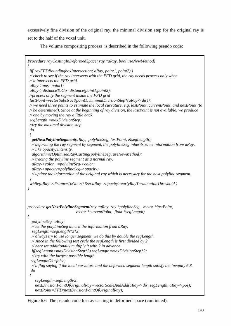
143

excessively fine division of the original ray, the minimal division step for the original ray is

set to the half of the voxel unit.

The volume compositing process is described in the following pseudo code:

Procedure rayCastingInDeformedSpace( ray *aRay, bool useNewMethod){ if( rayFFDBoundingboxIntersection( aRay, point1, point2) ) // check to see if the ray intersects with the FFD grid, the ray needs process only when // it intersects the FFD grid. aRay->pos=point1; aRay->distanceToGo=distance(point1,point2); //process only the segment inside the FFD grid lastPoint=vectorSubstract(point1, minimalDivisionStep*(aRay->dir)); // we need three points to estimate the local curvature, e.g. lastPoint, currentPoint, and nextPoint (to // be determined). Since at the beginning of ray division, the lastPoint is not available, we produce // one by moving the ray a little back. segLength =maxDivisionStep; //try the maximal division step do { getNextPolylineSegment(aRay, polylineSeg, lastPoint, &segLength); // deforming the ray segment by segment, the polylineSeg inherits some information from aRay, // like opacity, intensity. algorithmicOptimizedRayCasting(polylineSeg, useNewMethod); // tracing the polyline segment as a normal ray. aRay->color =polylineSeg->color; aRay->opacity=polylineSeg->opacity; // update the information of the original ray which is necessary for the next polyline segment. } while(aRay->distanceToGo >0 && aRay->opacity>earlyRayTerminationThreshold )}

procedure getNextPolylineSegment(ray *aRay, ray *polylineSeg, vector * lastPoint, vector *currentPoint, float *segLength){ polylineSeg=aRay; // let the polyLineSeg inherit the information from aRay; segLength=segLength*2*2; // always try to use longer segment, we do this by double the segLength. // since in the following test cycle the segLength is first divided by 2, // here we additionally multiply it with 2 in advance if(segLength>maxDivisionStep*2) segLength=maxDivisionStep*2; // try with the largest possible length segLengthOk=false; // a flag saying if the local curvature and the deformed segment length satisfy the inequity 6.8. do { segLength=segLength/2; nextDivisionPointOfOriginalRay=vectorScaleAndAdd(aRay->dir, segLength, aRay->pos); nextPoint=FFD(nextDivisionPointOfOriginalRay);

Figure 6.6 The pseudo code for ray casting in deformed space (continued).

144

if( isPointColinear(lastPoint, currentPoint, nextPoint ) ) // the three points are colinear, the division is ok. { segLengthOk=true ; l=distance(nextPoint,currentPoint); } else // we need to check the curvature radius {

r=curvatureEstimate(lastPoint, currentPoint,nextPoint); l=distance(nextPoint,currentPoint); // evaluate the chord length of the next polyline for the deformed ray

if( 2d2rd2l −≤ ) segLengthOk=true ; // when the inequity 6.8 is satisfied, the division is ok. } } while (! segLengthOk && segLength > minDivisionStep ) // the division of the original ray is repeatedly tested till the condition in equation 6.8 is satisfied // or segLength becomes too small. polyLine->distanceToGo=l; polyLine->dir=vectorSubstract(nextPoint, currentPoint); vectorNormalize(polyLine->dir); // The polyline will be processed as a normal ray, so let us treat it as a “ real” ray, // i.e. add information like distanceToGo, direction etc LastPoint=currentPoint; currentPoint=nextPoint; // get ready for processing of next polyline moveRayForword(aRay, segLength); aRay->distanceToGo-=segLength; // the original ray proceeds.}

Figure 6.6(cont.) The pseudo code for ray casting in deformed space.

The function algorithmicOptimizedRayCasting() is the same as that in figure 4.23, but

three modifications are made to enable correct rendering. One modification is for correct

shading calculation which is discussed in next section, the other two modifications are for

opacity compensation.

After the volumetric object is deformed, the intensity distribution within the volumetric

object is changed, therefore, the opacity per unit length along the deformed ray should be

compensated. The volume change caused by the deformation is given by the determinant of

the Jacobian matrix of the deformation function [59, 127]. Since the deformation is defined by

a B-spline FFD, as discussed in the next section, we can describe the local deformation

function with a linear transformation matrix T. In this case, the Jacobian matrix of the

deformation function is the linear transformation matrix itself. We can therefore directly use

the determinant of the linear transformation matrix T to adjust the opacity of a sample point.

145

Assume the sample space is ∆s. Assume also that before deformation the local

absorption coefficient at a sample point is k. According to equations 2.15, 2.17 and 2.20, the

sample point opacity is

skoriginal e ∆⋅−−= 1α 6.19

Assume the determinant of the Jacobian matrix of the local deformation function is Jac.

After the deformation, the local absorption coefficient will become k/Jac. Hence, the

deformed sample point opacity is

Jacoriginal

Jacskdeformed e /1/ )1(11 αα −−=−= ∆⋅− 6.20

The opacity compensation for volume change is implemented by using a 2D LUT to

avoid the computation of the power function in equation 6.20. One index of the LUT is for the

original opacity, the other index of the LUT is for the determinant of the Jacobian matrix.

Figure 6.7 Mismatch of deformed ray segments to the standard sample unit.

The other opacity compensation is for the mismatch of the deformed polyline length to

the standard sample unit. Since the deformed polylines have arbitrary length, there is no

guarantee that the length of each polyline segment is exactly a multiple of the standard sample

unit. In general, the last sample interval is shorter (see figure 6.7). For simplicity, assume that

the local absorption coefficient at a sample point is k (after the opacity compensation for

volume change), the standard sample space is ∆s, and the actual length of the last sample

original ray

deformed ray segments

146

interval is s′∆ . The non-compensated opacity for the last sample interval is then given by

equation 6.19. The actual opacity should be

s

s

originals

ssksk

actual ee ∆∆

∆∆

∆∆ αα′′

⋅−′⋅− −−=−=−= )1(1)(11 . 6.21

To compensate the length mismatch of the last sample interval to the standard sample

space, we use the same opacity compensation LUT as for the volume change. The only

difference is that the second index of the LUT is the ratio between the actual sample interval

and the standard sample space instead of the determinant of the Jacobian matrix.

Our opacity compensation approach for the mismatch of the deformed polyline length to

the standard sample unit is similar to the scheme proposed by Lacroute [6] which

compensates the opacity for different sampling spaces caused by the change of the viewing

direction in the shear-warp algorithm. The Jacobian-based opacity compensation for the

volume change is novel.

Notice that the opacity value of the last sample point is compensated twice: once for the

volume change, once for the mismatch of the actual sample interval to the standard sample

space.

6.3 Shading in the Deformed Space As discussed in chapter 2, the Phong shading model requires the normal vector at each

sample point to calculate the shading calculation. When the volume object is deformed, the

surface normal is also changed. Therefore we need a method to recalculate the local normal

vector.

For the 3D texture mapping based deformation methods [120, 121], the normal vector in

the deformed space is difficult to estimate. Since the volume is presented by slices of the

texture planes, there is no way to retrieve the 3-dimensional normal vector from the 2-

dimensional texture planes. Westermann et al. [121] used a pseudo illumination method for

the deformed volume in his 3D texture mapping based algorithm. The diffuse lighting

component is simulated by the forward difference of the scalar material of the texture volume

with respect to the light direction. This method requires a two pass rendering: each slice is

rendered twice, the second time the texture coordinates are slightly shifted in the light

direction and the fragment values are subtracted from the result of the first rendering. In

147

addition, the image rendered with this gradient-less shading method suffers from the increased

artifacts which may be caused by the difference operation (figure 6.8).

Figure 6.8 Deformed head rendered via 3D texture mapping by Westermann et al. [121]. Theleft is directly rendered. For the image on the right the diffuse illumination is simulated byforward difference.

Kurzion and Yagel [60] suggested to estimate the normal in the ray deflectors by using

the mapping of three points in the neighborhood of a sample point in the undeformed space to

construct a normal transform matrix, but they did not give any experimental result. In fact, the

approach suggested by them is not practical. It might be very complicated to implement the

normal transformation when multiple deflectors are used to simulate complex deformations

(since a point may be transformed by several deflectors, the normal needs to be transformed

correspondingly several times). In addition, they also have discontinuous ray deflectors. For

the sample points which are located in discontinuous neighborhoods, the transformation

matrix can not correctly be calculated in this way.

As discussed in chapter 5, the deformed normal vector can be estimated by applying the

Jacobian matrix of the deformation function on the original normal vector. Theoretically, for

our FFD-based volume deformation method, we can calculate the deformed normal vector by

analytically evaluating the Jacobian matrix of the deformation functions, since the

deformation is well defined by B-spline functions. However, the overhead of calculating the

Jacobian matrix with an analytical approach is huge [124].

We can reduce the required computation by exploiting the continuity of the deformation.

In our deformation approach, we use the B-spline basis function of degree 3, therefore the

deformation achieves C1 continuity. This allows us to assume that the transformation from the

undeformed space to the deformed space is linear in a small neighborhood of the sample

148

point. We can therefore estimate the local deformation function by checking the deformation

of three independent points in a small neighborhood of the current sample point. After that,

we can directly transform the local normal by deriving the Jacobian matrix of the local

deformation function as suggested by Barr [59].

Assume that the neighborhood dimension is δ, the current sample point is

T)z,y,x(P = , the three selected points in the δ-neighborhood of the current sample point P

are Tz

Ty

Tx )z,y,x(P,)z,y,x(P,)z,y,x(P δδδ +=+=+= . The counterparts of these

points in the deformed space are denoted by ffdy

ffdx PP and ffd

zP separately. Let T denote the

transformation matrix of the deformation function, thus we have

( ) ( )zyxffd

zffd

yffd

x PPPTPPP = 6.22

and

( )( ) 1−= zyxffd

zffd

yffd

x PPPPPPT . 6.23

To calculate the shading correctly with respect to the original ray, the normal estimated at

a sample point of the deformed ray must be transformed back by using the transpose of the

inverse Jacobian matrix of the deformation function. Since the deformation is assumed linear

in the local neighborhood, the Jacobian matrix of the deformation function equals the

transform matrix of the deformation function. Therefore the sampled normal vector can be

transformed backward into the deformed space by the following formula,

sample1nTn

�� −= 6.24

The inversely transformed normal vector n�

can then be used for shading calculation using the

Phong illumination model. The determinant of T describes the amount of volume change. It is

used for the LUT-based opacity compensation described in section 6.2.4.

Theoretically the transform matrix of the deformation function T may not be revertible

under some conditions. For example, if the deformation makes the point ffdxP superpose with

ffdzP or ffd

zP (this means that different parts of the volume interpenetrate each other), T is a

singular matrix, thus the normal vector can not be adjusted by formula 6.24.

149

One solution to this problem is to simply reject the movement of those FFD control

points which may lead to the interpenetrating of different volume parts. However, this

solution is impractical, since the detection of interpenetrating of objects is a computational

overhead [159].

As an alternative approach we can use extrapolation to calculate the intensity of a sample

point where the transform matrix of the deformation function T is not revertible. For each ray

we always store the intensity of the last two sample points. If the transform matrix of the local

deformation function at a sample point is revertible, we calculate the intensity of the sample

point using the Phong shading function with the adjusted normal vector; otherwise, we

calculate its intensity by linear extrapolation of the buffered intensity of the last two sample

points. This strategy is similar to the Gouraud shading which generates continuous lighting

effects. However, since the intensity is estimated by extrapolation instead of interpolation, we

have to clamp the extrapolated intensity to prevent the occurrence of unrealistic intensity

values, e.g. a negative intensity value.

6.4 Rendering Deformable and Undeformed Objects

in the Same Scene.In some applications, especially in surgical simulation, deformed and undeformed

objects may co-exist in the same scene. Therefore, simultaneous rendering of both deformed

and undeformed objects should be supported. We implement the simultaneous rendering of

both deformed and undeformed objects through an extra test of ray-object intersection. In the

rendering procedure, before traversing along the deformed ray path, the original ray is

checked to see if it intersects with the undeformed object. If no intersection exists, the ray-

casting is done using only the deformed ray trajectory. Otherwise, as indicated in figure 6.9,

for the ray segment before the intersection point, ray-casting is done along the deformed ray

trajectory. For the ray segment located inside the undeformed object, ray-casting is done

along the undeformed ray. The contribution of each ray segment is combined using α-

blending techniques [107].

150

aainv

b

binv

c

cinv

d

dinv

original sight ray

deformed ray path

Figure 6.9 Ray-casting the deformable and undeformable objects in the same scene. Thetrajectory followed by the ray casting procedure in the figure is ainvbinv+bc+cinvdinv

The result of rendering the deformable and undeformable objects in the same scene is

demonstrated in figure 6.10. Two objects are visible in the scene: a human jaw (2562×128

voxels) and a voxelized stick. The deformation of the jaw is defined by a FFD grid and the

stick is defined as an undeformable object in the scene. The images show that the stick

remains undeformed in the rendered images while the human jaw is deformed with increasing

magnitude. The results confirm the validity of our simple strategy for the rendering of both

deformable and undeformable objects in the same scene.

Figure 6.10 Result of ray-casting the jaw (deformable) and a stick (undeformble)simultaneously. The stick stays undeformed, while the jaw is deformed with differentdeformation amplitudes.

151

6.5 Algorithmic Optimizations As we discussed in the previous chapters, algorithmic optimizations are key approaches

to improve interactivity of volume rendering. However, till now the algorithmic optimization

for volume rendering of deformable objects is not addressed by any researcher.

If the ray casting acceleration methods can be integrated into our inverse-ray-

deformation-based algorithm, the rendering of deformable objects would be double-fold

accelerated, since the time saving comes not only from the decrease of the volumetric

compositing operations, but also from the saved deformation operations for the sample points.

Fortunately, all of the ray casting acceleration techniques that we applied in chapter 4 can

be implemented in the new rendering algorithm for the deformable volume.

In our rendering scheme, the deformed ray is approximated by polylines. When the ray

trajectory is followed during the rendering process, it samples the original volume equal-

distantly along the polyline segments. Hence, the encoded distance values for both space-

leaping and coherence acceleration are still usable. There is only one restriction: the leap

distances and the coherence distances must be trimmed if they are longer than the length

between the current sample point and the end point of the polyline segment. In addition, early-

ray-termination can still be implemented by checking the opacity and thus stopping the

processing of the current ray if the accumulated opacity exceeds a user-defined threshold.

Since the polyline segments of the deformed ray are followed in front-to-back order, the ray

information like opacity and intensity are propagated when the ray is followed from one

polyline segment to another.

6.6 Experimental Results and Analyses We tested the new algorithm with different volumetric data sets. In the experiments we

rendered the volume objects with different deformation magnitudes and opacity transfer

functions. We achieved appealing deformation effects in terms of image quality. Images in

figure 6.11 are examples of ray casting results of CT head and Engine. Notice that in the CT

head data, the CT metal artifacts are not filtered1. Their appearance, however, as can be seen

1 On how to reduce the metal artifacts in CT images refer [160] and [161].

152

in image b, helps to demonstrate the smoothness and continuity of the deformation thanks to

the adaptive division of the ray segment length.

Figure 6.11 Example rendering of undeformed and deformed volume objects. a) Theundeformed CT head. b) The deformed CT head. c) The undeformed engine. d) Thedeformed engine.

a) b)

c) d)

153

We found that the shading adjustment is very important for the correct display of the

deformed shapes of the volume objects. This can be demonstrated by comparing the rendering

results of volume objects with shading adjustment to the renderings without shading

adjustment. The comparison is presented in the figure 6.12 (more rendering results are listed

in appendix A). The images on the left column were rendered without shading adjustment,

while the images on the right column were their counterparts rendered with the shading

adjustment. As demonstrated by these images, without shading adjustment, the result images

are confusing, although the profiles of the deformed object are correct. Only with the shading

adjustment the deformed volume can be illuminated correctly.

In our volume deformation algorithm, the shading is gradient-based. The result image

quality is therefore superior compared to other volume deformation approaches which use

gradient-less shading calculation. For example, compared to the images rendered by the 3D

texture mapping based method (see figure 6.8) which uses pseudo diffuse illumination, our

method can more correctly reveal the deformed shape of volume objects, and the images

rendered by our method are artifact-free (here we mean image artifacts, not the CT metal

artifacts which are inherent in the data sets), while the artifacts in figure 6.8b are very

noticeable due to the use of the difference operation required by the pseudo diffuse

illumination.

Figure 6.12 Comparisons of deformation without and with shading adjustment (continued).

a) b)

154

Figure 6.12 (cont.) Comparisons of deformation without and with shading adjustment. Imagea, c, and e are rendered without shading adjustment, while image b, d and f are rendered withshading adjustment.

The shading adjustment requires extra calculations to determine normal vectors. For each

sample point, we need to additionally deform three adjacent points in order to calculate the

normal transform matrix. Therefore the shading adjustment increases the total rendering time

considerably. Table 6.1 is the comparison of the rendering times for different data sets.

As can be seen in table 6.1, the rendering time with shading adjustment are 3.33~5.80

times longer than the rendering time without shading adjustment due to the extra operations

for the normal transformation. Since the correct shading is very important, however, we have

to accept the increase of rendering time.

c) d)

e) f)

155

Rendering time (seconds)

volume data sets case A: without

shading adjustment

case B: with

shading adjustment

Ratio of rendering

time (B/A)

MRI Brain 5.25 26.56 5.05

Heart 5.62 28.19 5.01

Engine2 6.42 37.27 5.80

CT head 10.59 44.79 4.22

Jaw(opaque) 4.06 16.77 4.13

Jaw(semi-transparent) 11.50 38.34 3.33

Table 6.1 Comparison of rendering times between two shading schemes.

We observed that the contribution of algorithmic optimization techniques to the

acceleration of the volume deformation is still considerable. As the statistic results in table 6.2

show, the algorithmic optimized deformation algorithm is 2.34~6.56 times faster than the

brute force method.

rendering time (seconds)volume data sets

case A: non-optimizedrendering algorithm

case B: optimizedrendering algorithm

Ratio ofrenderingtime(A/B)

MRI Brain 62.20 26.56 2.34

Heart 65.87 28.19 2.34

Engine2 118.23 37.27 3.17

CT head 127.18 44.79 2.84

Jaw(opaque) 109.96 16.77 6.56

Jaw(semi-transparent) 108.02 38.34 2.81

Table 6.2 Comparison of rendering times between the optimized algorithm and the brute forcealgorithm.

However, the speedup factors are noticeably lower than the achievable speedup factor in

rendering undeformed objects. As we know, the combination of the different algorithmic

optimization techniques can usually speed up the rendering of static (undeformed) volume

156

objects with a factor up to 10 or even more. What leads to this decrease of speedups while the

used algorithmic optimization methods are the same ones?

The main reason is that we integrate the more computationally expensive deformation

operation in our rendering procedure. The rendering related operations, like volume

resampling and compositing, are relatively cheaper than the deformation operations, since the

deformation of each point requires to blend the contribution of 64 involved FFD control

points (we used degree 3 B-spline functions). Moreover, we need to deform three additional

points in the neighborhood of the current sample position in order to calculate the normal

transformation matrix for the shading adjustment. Although the space-leaping and the

coherence acceleration can save the rendering related operations, they do not save the

expensive computations for the ray segments deformation. Only early-ray-termination can

simultaneously save the computation for rendering and deformation. Thus the space-leaping

and the coherence acceleration is not as efficient in the volume deformation procedure as in

rendering static volume objects.

Another factor that makes the algorithmic optimizations less efficient is the limitation of

the segment length of polylines which approximate the ray trajectory in the deformed space.

We render the deformed volume by following the piecewise linear segments of polylines.

When the distance for space-leaping or for spatial coherence acceleration is longer than the

length of the polyline segment, the distance is replaced by the length of the polyline segment.

When the deformation is severe, the average length of the polyline segments will be decreased

to match the deformation, this will make the actual average distance for space-leaping and

coherence acceleration shorter than the encoded distance, leading to the efficiency decrease of

the algorithmic optimizations.

We examined the impact of the deformation amplitude on the performance of our

deformation approach. To measure the performance, we used three values: the average length

of polyline segments, the average number of non-transparent sample points per ray

(sampling/ray), and the average times to fetch the distance for space-leaping and coherence

acceleration (distance/ray). We achieved similar results for different data sets. We present and

analyze here only the results for the volume data engine. In the experiments, a semi-

transparent mapping and two different opaque mappings differing in the percentage of empty

space in the volume are tested.

The curves in figure 6.13 show the performance change of the deformation rendering

algorithms with respect to the deformation amplitude.

157

Figure 6.13 The impact of the deformation amplitude on the algorithm performance.

a)

b)

c)

d)

semi-transparentmapping

opaque mapping

opaque mappingwith empty space

158

In the current implementation, the polyline segments of the deformed ray have a length

between 0.5 and 8. As discussed in section 6.2.4, we use a minimal polyline segment of 0.5

voxel size to prevent the meaningless subdivision of rays, while 8 is the interval between

points on the FFD grid. According to figure 6.13a, the average length of the ray segments

decreases with the increase of the deformation magnitude from 8 to a value of about 2.0. It

shows how the ray is adaptively divided into smaller segments to match the deformation

magnitude. The extra computation necessary for deforming the viewing ray therefore does not

increase further when the limiting value of the average length of ray segments is approached.

The curves in figure 6.13b show the performance change of the deformation approach

without algorithmic optimization. For the non-optimized ray casting the opacity mapping has

no impact on the performance. Therefore, the curves in figure 6.13b are identical for all three

different opacity mappings. However, the samples per ray increase almost linearly as the

deformation becomes more severe, because the ray trajectory becomes longer when the

deformation amplitude increases. The volume, however, is still resampled equal-distantly.

On the contrary, for the optimized method, the impact of the opacity mappings on the

performance is quite different from the non-optimized method. As shown in figure 6.13c, the

increase of sampling/ray is only gradual. Theoretically, there should be no increase of

samples/ray when we use algorithmic optimizations, because the increase of the ray trajectory

length in the deformed space does not change the condition for early-ray-termination.

Nevertheless, in our deformation approach, we adjust the opacity values of the sample points

in order to compensate the density change caused by the deformation. This might increase the

required sample point number. Furthermore, since the length of the deformed ray segment is

often not an exact multiple of the sampling distance, the length for the last sampling interval

is usually shorter than the standard sampling distance (which is compensated as described in

section 4.2.4). This leads to additional samples and increases the number of samples/ray with

the deformation. This is more striking for the semi-transparent mapping, because for each ray,

a longer path through the volume must be traversed before the accumulated opacity of the

viewing ray exceeds the threshold for early-ray-termination. In addition, for the semi-

transparent mapping, the coherence acceleration may not be as efficient as in rendering

undeformed objects, since the coherent distance is limited by the length of the polyline

segment. The increase of sampling/ray for the semi-transparent mapping is thereby more

noticeable than the one for the opaque-empty mappings.

On the other hand, the effect of the deformation amplitude on the efficiency of space-

leaping and coherence acceleration is more severe than early-ray termination. Figure 6.13d

159

shows that severe deformation leads to higher number of the distance/ray, and therefore

lowers the efficiency of space-leaping and coherence acceleration. This can be explained

again by the limitation of the polyline segments. When the deformation amplitude increases,

the average polyline segment length decreases. In this case, it is more likely that the actual

distance for space-leaping or coherence acceleration is trimmed by the polyline segments.

Consequently, more additional shortened leaps are necessary to cover the same length of ray

trajectory. The influence of the average length of ray segments on the efficiency of space-

leaping and coherence acceleration can be observed very clearly if we compare figure 6.13a

with figure 6.13d. If the deformation amplitude is between 0-25, the average length of ray

segments decreases dramatically from 8 voxel units to about 2 voxel units. Correspondingly,

the distance/ray increases dramatically. As the average length of ray segments approaches its

converging value, the distance/ray increases linearly with the deformation, since the length of

the ray increases linearly as well.

We list the acceleration rates of the algorithmically optimized deformation method with

respect to the non-optimized method under different deformation magnitudes in terms of

samples/ray in table 6.3, where each operation for retrieving a distance value for space-

leaping is also counted as a normal “sampling” operation, although the operation for the

empty samples is cheaper than the operation for the non-empty ones (the former simply

moves the ray to the next sample point, the latter resamples the volume, accumulates the

sample contribution, and adjusts the shading value). During the deformation, the FFD control

points are shifted by two sine functions, making a circle wave on the volume (see figure 6.12).

The deformation magnitude is given by the amplitude of the sine function.

Deformation magnitudeSetting of engine’s opacity

0 15 30 45Semi-transparent 4.43 3.29 3.13 3.23Opaque-empty 13.70 7.11 6.23 6.20

Opaque-empty with more empty space 14.16 5.10 4.67 4.52

Table 6.3 Ratios of overall sample numbers between the non-optimized deformationalgorithm and the optimized deformation algorithm.

As shown in the table, when there is no deformation, the acceleration rate for the

opaquely mapped volume, which has a lot of empty space, is 14.16. This is much higher than

the acceleration rate for the semi-transparently mapped volume, which is 4.43. For semi-

transparent objects the speedup factor decreases only gradually, while for opaque scenes

160

which have larger empty regions, there is a significant decrease of a factor between two and

three. This shows that the deformation has its main effect on space-leaping due to the

limitation of the space-leaping distance by the segment length.

We found that our adaptive ray division method for the approximation of the ray trajectory

in the deformed space is a guarantee to make the deformation spatially continuous. Figure

6.14 shows the deformation of Jaw rendered with three ray division strategies: image a and b

are rendered by dividing the original ray into equal-distant intervals with length of 4 voxel

units and 2 voxel units separately, while image c is rendered with adaptive ray division, the

average interval length being 1.9. The same deformation amplitude and camera settings are

used when rendering these images. Image d is a reference image in which the jaw is not

deformed. As marked by the arrows in the images, in the heavily deformed regions, even with

a small division interval of 2 voxel units, the deformation is not continuous due to the

mismatch of the division interval length to the local deformation amplitude. In contrast, the

deformation in these regions is continuous when we use the adaptive division approach.

Figure 6.14 Comparison of ray division methods. a) Using fixed division intervals of 4 voxelunits. b) Using fixed division intervals of 2 voxel units. c) Using adaptive ray division byconsidering local curvature. d) Reference rendition without deformation.

Obviously, more accurate approximations of the ray trajectory in the deformed space can

be implemented by using non-linear curve segments, so that a more continuous deformation

a) b)

c) d)

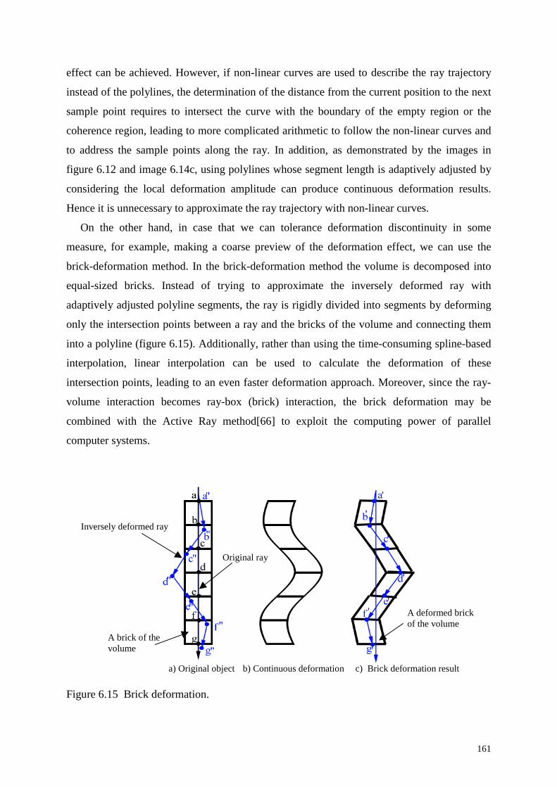
161

effect can be achieved. However, if non-linear curves are used to describe the ray trajectory

instead of the polylines, the determination of the distance from the current position to the next

sample point requires to intersect the curve with the boundary of the empty region or the

coherence region, leading to more complicated arithmetic to follow the non-linear curves and

to address the sample points along the ray. In addition, as demonstrated by the images in

figure 6.12 and image 6.14c, using polylines whose segment length is adaptively adjusted by

considering the local deformation amplitude can produce continuous deformation results.

Hence it is unnecessary to approximate the ray trajectory with non-linear curves.

On the other hand, in case that we can tolerance deformation discontinuity in some

measure, for example, making a coarse preview of the deformation effect, we can use the

brick-deformation method. In the brick-deformation method the volume is decomposed into

equal-sized bricks. Instead of trying to approximate the inversely deformed ray with

adaptively adjusted polyline segments, the ray is rigidly divided into segments by deforming

only the intersection points between a ray and the bricks of the volume and connecting them

into a polyline (figure 6.15). Additionally, rather than using the time-consuming spline-based

interpolation, linear interpolation can be used to calculate the deformation of these

intersection points, leading to an even faster deformation approach. Moreover, since the ray-

volume interaction becomes ray-box (brick) interaction, the brick deformation may be

combined with the Active Ray method[66] to exploit the computing power of parallel

computer systems.

Figure 6.15 Brick deformation.

Inversely deformed ray

Original ray

a) Original object b) Continuous deformation c) Brick deformation result

A brick of thevolume

A deformed brick of the volume

162

The continuity of the brick deformation is affected by the brick size. Figure 6.16 are the

deformation results of a voxelized stick and Engine2 which are rendered by using adaptive

ray division and by using the brick deformation with different brick sizes. The brick

deformation produces jagged deformation results and the images have mosaic-like patterns.

As the images show, the annoying effect of jagged edges and the mosaic-like patterns in the

images can be suppressed by using smaller bricks, but smaller brick size will lead to more

computational overhead due to more frequent intersect-detection between the rays and bricks.

Figure 6.16 Comparison of deformation results.

The rendering times of the deformed stick and engine2 using different brick sizes are

listed in table 6.4. As reference, we list also the rendering time consumed by the adaptive ray

division based approach. When the brick size is 16×16×16, the rendering times for both stick

and Engine2 are about one quarter of the rendering times for the adaptive ray division based

method. As we decrease the brick size, the rendering time increases proportionally. When the

brick size is decreased to 4×4×4, the rendering times consumed by the brick deformation

a) Stick deformed by using b) Stick deformed by using c) Stick deformed by using adaptive ray division bricks (brick size 16×16×16) bricks (brick size 4×4×4)

d) Engine2 deformed by using e) Engine2 deformed by using f) Engine2 deformed by using adaptive ray division bricks (brick size 16×16×16) bricks (brick size 8×8×8)

163

become close to those consumed by the adaptive ray division based approach. Further

decrease of the brick size even leads to the brick deformation being slower than the adaptive

ray division based approach due to more frequent detection of ray-brick intersection. The

experimental results show that a reasonable brick size, which achieves faster deformation

without leading to unacceptable deformation effects, is about 8×8×8 voxel units.

Rendering time (seconds)Brick deformationVolume data Deformation by

adaptive ray division 16×16×16 brick 8×8×8 brick 4×4×4 brick 2×2×2 brick

Stick (2562×30) 20.38 5.02 8.64 16.12 30.99Engine2 (2562×110) 37.27 9.87 16.60 31.13 59.12

Table 6.4 The deformation times (in seconds) for different brick sizes.

6.7 Conclusions In this chapter we developed a new volume deformation algorithm which combines FFD

with inverse ray deformation. The deformation method is efficient, since it does not require to

deform the whole volume and generate an intermediate deformed volume before rendering

can be done.

We have shown that this new ray casting method has no problem to render deformable

objects and undeformable objects simultaneously in the same scene.

We developed the shading calculation approach in the deformed space. Unlike the

previous method which uses a gradient-less shading, the true Phong shading is implemented

in our method by backward transforming the normal vectors into the original volume space.

The rendering results show that the correct shading is very important for the shape display of

the deformed objects.

We designed a LUT-based method to compensate the opacity value of the sample points

by considering the local volume change, since the deformation changes the density

distribution inside the volume. The same LUT is used for the opacity compensation of the

possible mismatch of deformed ray segment lengths to the standard sample space.

We also developed an adaptive ray division approach for a precise approximation of ray

trajectories in the deformed space by considering the local curvature. Using this approach, the

simulated deformation is guaranteed to be spatially continuous.

Furthermore, we incorporated ray casting acceleration techniques in this new deformation

method, including the coherence acceleration developed in chapter 4. This is done by

approximating the continuous ray trajectory in the deformed space with piecewise linear

polyline segments. Experimental results show that the efficiency of early-ray-termination is

164

almost not affected by the deformation. For the space-leaping and spatial coherence

acceleration, due to the limitation of the ray segment length, their acceleration contribution

decreases when the deformation amplitudes are increased. Even so, we achieved speedup

factors between 2.34 and 6.56, compared to the non-optimized deformation procedure.

If deformation discontinuity is tolerable in some measure, for example, when we make a

coarse preview of the volume deformation procedure, we can also use the brick deformation.

In the brick deformation the ray is divided into polylines by ray-brick intersection. Using

larger bricks will reduce the operations of deforming the end points of polylines, hence we

can achieve even faster deformations at the cost of losing deformation continuity.

165

Chapter 7

Conclusions

7.1 Final Summary Volume rendering is a relatively new technique. It transforms the embedded

information in volumetric data sets into a visual form, and enhances our ability to understand

and manipulate three or higher dimensional data.

The huge size of practical volume data sets, however, results in a high computational

complexity, which is proportional to the volume size in brute force rendering algorithms, and

presents a memory bandwidth bottleneck. Hence, the volume rendering is computationally

intensive.

This dissertation has addressed two aspects of volume rendering: acceleration of

volume rendering and fast volume deformation.

The first part of the dissertation focuses on the rendering of static volume objects.

166

Space-leaping and early-ray-termination are two popular acceleration methods which

are used to accelerate the shear-warp algorithm and the ray-casting algorithm. However, these

two methods are efficient only if the voxels in the volumetric object are either opaque or

transparent. If the portion of semi-transparent voxels in the volume is large and empty space

in the volume is not present, the performance of a rendering system which uses only these two

techniques will considerably degrade [8]. We observed that the opacity coherence in the

volume data can be exploited to minimize this opacity-transfer-function-dependent

performance instability.

The coherence acceleration reduces the unnecessary memory access and resampling

operations by processing only two voxels at the ends of each coherent segment. The

information for the voxels within the coherent regions is derived by cheaper 1D interpolation.

We found that the coherence acceleration does not evidently accelerate the shear-warp

algorithm, even when the average coherence distance is as high as 12 voxel units. This is due

to the facts that shear-warp has high memory coherency by traversing the volume in memory

order, and the sampling filter kernel used in the shear-warp algorithm is 2-dimensional instead

of 3-dimensional, thus the 1D interpolation for the opacity of voxels within the coherent

regions is not necessary cheaper than directly sampling the volume.

Unlike the shear-warp algorithm, the ray-casting algorithm is an image order algorithm

for which the memory access is not efficient due to its irregular addressing arithmetic.

Moreover the operations for resampling the opacity of each sample point and shading

calculation in the ray casting algorithm is very expensive, and such operations need to access

the voxels in the neighborhood of sample points repeatedly, leading to more severe memory

bandwidth bottleneck problems. By reducing the tri-linear interpolation and shading

calculation in the coherent regions, the coherence acceleration technique can considerably

accelerate the ray casting process. This has been confirmed by our experimental results: we

achieved speedups between 1.9 and 3.5 times for different data sets. Therefore, we reached

the main goal of this work, i.e. speeding up the rendering of semi-transparently classified

volume about 2 times or more, so that the volume graphics engine can render arbitrary

classified volumes in real time.

Like the space-leaping techniques, the coherence acceleration requires the spatial

coherence information to be calculated in a preprocessing stage (abbreviated as EDC), so that

the speedup can be fully available in the rendering phase. The coherence distance, which is

stored with each non-empty voxel, is calculated view-independently, as the volume may be

viewed from different directions. The brute force EDC is unacceptably time consuming due to

167

the tremendous search space for the optimal coherence distance. We developed a Taylor-

expansion-based coherence encoding algorithm by converting the direct search of the local

coherent distance to the search of the local maximum of the second order partial difference of

opacity value. Although we underestimated the coherent distance by using the Taylor-

expansion-based EDC, the performance penalty for the ray casting process is small. Most

important, the processing time is reduced to a reasonable magnitude, i.e. for the data sets with

up to 2562×128 voxels, the coding time is less than 12 seconds. Since the regions where

space-leaping occurs do not superpose the coherent regions (the former is empty, while the

latter is non-empty), the encoded coherence distance does not consume extra memory

resources. Instead, the distance array for the space-leaping is shared by the coherence

distance.

We incorporated the new coherence acceleration algorithm with space-leaping and early-

ray-termination and implemented them in our ray casting program written in C++. The

visualizing parameters are adjustable via a parameter dialog window.

Furthermore, the coherence acceleration technique can be incorporated into the VGE

volume rendering pipeline with only slight modifications.

In brief, the main achievements made in the first part of this dissertation are:

• We developed a new ray casting acceleration technique. The new ray casting

acceleration technique speeds up the volume rendering of semi-transparent

volumes by a factor of 1.9~3.5, thus enables VGE to render arbitrary classified

volumes in real time.

• We proposed an efficient spatial coherence encoding algorithm. With the proposed

encoding algorithm, the preprocessing time is reduced to less than 12 seconds. This

makes the new ray casting acceleration technique usable in practice.

In the second part of this thesis we have concentrated on the deformation of a volumetric

object.

It is a very challenging task to deform volumetric objects, since the volume object is

presented by exhaustively enumerating each of its element primitives, i.e. voxels. Directly

mapping a voxel from the original object space to the deformed space is impractical due to the

prohibitive computational cost and the potential loss of details during the mapping process.

Instead, we used the inverse ray deformation to unify the volumetric object deformation

and the volume rendering process, avoiding the computational cost for reconstructing the

intermediate deformed volume. In addition, we also do not consume extra memory to store

168

the intermediate volume. Moreover, by integrating the object deformation procedure into the

volume rendering process, the voxels which do not contribute to the final image are not

considered at all.

Unlike the ray deflectors which need different pre-defined local transformation functions

for different deformation effects, we use the free form deformation. The FFD presentation is

based on uniform B-spline basis functions. The local property of B-spline functions allows the

shape of volume objects to be deformed locally; on the other hand, the locality means that the

deformation of any point in the deformed space is only affected by the control point located in

its neighborhood (the region of the neighborhood is determined by the degree of the B-

splines), thus the required computation is much less than the original Bézier function based

FFD which is global and must compute the contributions of all control points.

In the Kurzion’s implementation (ray deflectors), the inversely deformed ray is

approximated by dividing the original viewing ray equal-distantly and then transforming them

into consecutive polylines in the deformed space. Since the deformation amplitude varies in

the space during arbitrary deformation of objects, we adaptively divide the viewing rays to

match the local deformation amplitude, so that in the lightly deformed regions we can use

longer divisions of the ray to reduce the computation cost, while in the heavily deformed

regions shorter divisions can be automatically selected to prevent discontinuous deformations.

This involves the calculation of the local curvature. We developed a method for estimating the

local curvature of the deformed ray curve. The local curvature is used to guide the division of

the viewing ray, resulting in smooth deformations.

We also developed a shading calculation approach in the deformed space. Unlike the

previous method (by Westermann et al.) which uses a gradient-less shading, the true Phong

shading is implemented in our method by backward transforming the normal vectors into the

original volume space. The normal transformation matrix involves the computation of the

Jacobian of the deformation function. The computational cost to analytically calculate the

Jacobian matrix from the B-Splines is not acceptable. We assumed that the deformation

function is linear in a small neighborhood of the sample point, allowing the estimation of the

deformation function by additionally deforming three extra points in the neighborhood of the

sample point. In this way, we saved considerable time for the normal estimation.

After deformation, the volume of the original object is changed, leading to the change of

the density distribution inside the volumetric object. We designed a LUT-based method to

compensate the opacity of the sample points by considering the local volume change which is

described by the determinant of the Jacobian matrix of the local deformation function. Since

169

the Jacobian matrix is calculated during the shading adjustment, the additional operation for

the opacity compensation is limited.

Finally, we have incorporated ray-casting acceleration techniques in this new

deformation method. The time savings by the ray-casting acceleration techniques in the

volume deforming process are twofold: the deformation of the reduced sample points and the

resampling as well as shading of the reduced sample points. Experimental results show, in

addition to the computational savings for the generation of an intermediate deformed volume,

that the ray casting acceleration techniques can provide an additional speedup factor of 2.34 to

6.58.

The achieved deformation effects are very appealing compared to the results by others.

To sum up, the contributions in the second part of this dissertation are:

• We combined the traditional free-form-deformation with the inverse-ray-deformation.

Such a combination allows volume objects to be deformed into arbitrary shape, while the

calculation and the memory space for generating and storing a intermediate deformed

volume are saved.

• We proposed an efficient method for the estimation of the local deformation function

which is used to adjust shading and opacity in the deformed space.

• We proposed an approach for rendering deformed volume objects and undeformed objects

in the same scene.

• We developed an adaptive ray division algorithm by considering the local curvature along

the deformed rays. Thus deformation calculation in the slightly deformed region is

reduced without loss of the spatial continuity of the simulated deformation.

• We adapted the ray casting acceleration techniques in the new deformation algorithm and

achieved a speedup factor of 2.34~6.56 in rendering heavily deformed volume objects.

7.2 Future Directions The extension of the current work will include three aspects.

First, we observed that in the coherent regions the absorption function as well as the

opacity could be described by linear functions, thus the contribution of such a coherent

segment along a ray can be analytically evaluated by a numerical approach, e.g. using the

Simpson-formula which requires only three sampled values. In this way, the required

computation for each coherent segment will be fixed and independent of its length. In our

170

current ray casting algorithm this is not implemented. However, for hardware implementation,

the computational cost for composing the contribution of each coherent ray segment should be

independent of its coherence length, so that the rendering pipeline can work at full speed.

Therefore, it is worthy to study the performance of the numerical approach.

Second, the present deformation is still slow. The main overhead comes from the normal

transformation. In order to derive the normal transformation matrix, we need to know the

deformation of three additional points in the neighborhood of each sample point. The

overhead of the normal transformation can be reduced by exploiting neighborhood coherence

again. This can be implemented by using a buffer to store the deformed points. When any

sample point and its three adjacent points are deformed, their deformed coordinates can be

stored in the buffer. Thus, before really deforming a point, we can check the buffer to see if

the point is deformed by previous rays or sample points. When the deformed point is found in

the buffer, we need not bother to deform it again, since the deformation is very expensive.

Finally, we use a B-spline FFD grid to define the deformation at present. The volume

deformation is defined by changing the control points of the FFD grid. The control points of

the FFD grid are moved by space functions or by interactively adjusting coordinates, thus the

deformation is not driven by physical laws. We plan to incorporate physical laws to guide the

deformation procedure. This can be implemented by combining the FFD with other physical

deformation models, like Mass-Spring systems or FEM. In fact, the FFD is suitable to be

combined with such physical deformation models [122, 144]. With current technologies the

deformation using a Mass-Spring system or other simplified FEM variations can be

implemented in real time [138]. So we plan to combine the Mass-Spring system and the FFD

grid into a generator of space deformation, thus developing a complete volume deformation

system which exploits the high efficiency of the inverse transformation based ray casting

approach proposed in this thesis to deliver volume deformation with interactive speed. Such

“automatic” deformation systems can be used e.g. to simulate a beating heart.

171

Appendix A

Rendering Results

A1: Rendering results of human jaw (2562×128 voxels), the images on the left are renderedwith early ray termination, space leaping and the spatial coherence acceleration; the imageson the right are rendered only with early ray termination and space leaping.

Human jaw with many voxels semi-transparently mapped.

Human jaw in which the voxels are mapped either empty or opaque.

172

A2: Rendering results of CT head (2562×113 voxels), the images on the left are rendered withearly ray termination, space leaping and the spatial coherence acceleration; the images on theright are rendered only with early ray termination and space leaping.

CT head with many voxels semi-transparently mapped.

CT Head in which the voxels are mapped either empty or opaque.

173

A3: Rendering results of MRI Brain (1282×84 voxels), the images on the left are renderedwith early ray termination, space leaping and the spatial coherence acceleration; the imageson the right are rendered only with early ray termination and space leaping.

MRI Brain with many voxels semi-transparently mapped.

MRI Brain in which the voxels are mapped either empty or opaque.

174

A4: Deformation results of MRI Brain (1282×84 voxels)

Original Brain

Deformed without shading adjustment

Deformed with shading adjustment

175

A5: Deformation results of Heart (202×132×144 voxels)

Original heart

Deformed without shading adjustment

Deformed with shading adjustment

176

177

Appendix B

The Volume Ray Casting and

Deformation Program

B.1 Program Structure Overview

The program for the accelerated ray casting and volume deformation is written in C++ and has a

simple hierarchical structure as shown in figure B1.

The top of the hierarchy is a graphical user interface implemented by Qt. The user graphic

interface is implemented by a class named ImageViewer. The class ImageViewer is derived from

the Qt widget class QmainWindow. The user commands, like load volume data, set viewing

parameters and rendering parameters, render etc., are issued through three dialog pads, tool-

buttons or menus of the main window. The rendering results are also displayed in the two image

frames of the main window.

178

Figure B1 Program structure overview of volume ray casting and deformation.

Under the user-interface is a class Scene. The ImageViewer has an instance of the class

Scene. The member variables of the class Scene include the parameters for volume classification,

shading calculation, viewing matrix, lighting, etc. The most important members are Volume and

SplineGrid. Most of the member variables have default values for convenience, but they can be

also explicitly initialized by calling corresponding public member functions. Public member

functions like addVolume(..), addSplineGrid(...) addLight(...) must be explicitly called before the

execution of the rendering function renderExtendedNew(...). The function renderExtendedNew()

generates an image by casting rays into the virtual scene in quite the same way as the traditional

ray tracers do, except that the volume is equal-distantly resampled and the contribution of the

sample points is accumulated by the over operation.

Two parallel classes, Volume and SplineGrid, are located in the third level of the hierarchy.

The Volume contains the 3D scalar volume data and a distance array. The availability of the

distance array is indicated by a boolean member variable distanceArrayAvailable. Whenever the

volume data is first loaded or the volume classification parameters are changed by the user, the

distanceArrayAvailable is set to false and hence the member function distanceCoding() is called

to update the distanceArray at the beginning of the rendering process.

The class SplineGrid is used for deformation description. The SplineGrid contains a grid of

FFD control points. The control points are currently not moved in an interactive or physically-

User Interface (Qt)

Scene

Volume SplineGrid Light

Miscellaneous variables, suchas visualization parameters,

rendered image etc.

179

based automatic way, but are moved by using specific space functions. The most important

member function of the SplineGrid is deformExtendedRay(...). By calling this function the

straight viewing rays are inversely deformed in the deformed space. By following the inversely

deformed ray the deformed volume can be rendered without really generating an intermediate

deformed volume.

B2. Classes and Data Types SpecificationB2. 1 ImageViewer:

A derived class from Qt widget class MainWindow.

member variables:

int volSizeX, volSizeY, volSizeZ; //define volume size.

Vector3 volPos, volRo; // define volume position and orientation (rotation).

Qstring volumeName; // file name of the loaded volume data.

Vector3 viewPos; // define the viewer position.

Scene theScene; // an instance of the class Scene.

int viewMode; // define project mode, perspective/parallel.

ParameterDiag paraSetter; // dialog pad for miscellaneous parameter adjustment.

int oriDataType; // indicate the original data type of volume, 8/16 bits.

Color lightColor; // light color;

Vector3 lightPos; // light position;

int LTh, HTh, highOp; // volume classification parameters, the density values

// between 0 and LTh are mapped to zero; the density

// values between LTh and HTh are linearly mapped to

// the range between 0 and highOp; the density values

// greater than HTh are linearly mapped to the range

// between highOp and 1.

double allowedErr; // error threshold for distance encoding.

double earlyTermTh; // opacity threshold for early-ray-termination.

int gridSize; // subcube size for the SplineGrid.

int deformType; // indicate whether volume is deformed or not,

// possible value is NODEFORM (0) or FFD (1).

int analysePerformance; // indicate whether to report the performance related

180

// statistics or not, The statistic include the distance/ray,

// sample/ray, rendering time etc.

int compareMethods; // if true, then render two images by using new algorithm

// and old algorithm separately.

int codingStyle; // 0 for brute force EDC, 1 for Taylor Expansion-based

// EDC;

int subSampleNums; // sample numbers per voxel unit, usually 2.

int classifyParaChanged; // if true, the member function distanceCoding() of

// Volume will be called before rendering;

int FovH, FovV; // field of view for horizontal and vertical directions.

Color bkColor, // background color.

Color trnsColor, opaqueColor; // colors for semi-transparent voxels and opaque voxels.

int ImgSizeX,ImgSizeY; // define output image dimension.

ExtraOptions *extraOptions; // a dialog to set parameters for additional options, like

// codingStyle, subSampleNums, compareMethods,

// deformType, analysePerformance etc;

Important member functions:

ImageViewer( QWidget *parent, const char *name, int wFlags );

// the construction function.

~ImageViewer(); // destructs the ImageViewer object and frees all allocated

// resources.

void initializeScene(); // generate an instance of the class Scene, namely

// theScene, initialize theScene with the selected

// parameters like the view matrix, light, volume etc. by

// calling the public member functions of theScene.

void initParaDiag(const char * fileName);

// It is called when a volume is loaded into memory from a

// file, it generates an instance of the class ParameterDiag ,

// namely, paraSetter. Through paraSetter the volume

// classification and visualization parameters are adjusted.

void openFile(); // load volume data from a file. After the file name is

// selected by calling the QFileDialog::getOpenFileName(),

// it sequentially calls the member functions initParaDiag()

181

// and initializeScene();

void render(); // generate the image of the volume. If no volume is loaded,

// it does nothing; Before rendering, it checks whether the

// distance array of the volume matches the classification

// parameters. If not, the volume member function

// distanceCoding() will be called before rendering.

void loadImage(); // read the rendered image from theScene and display it.

B2. 2 Scene:

A base class.

member variables:

ExtendedRay *castedExtendedRay; // a ray pointer used for ray casting.

int codingStyle; // distance coding method, 0 for brute force EDC, 1 for

// Taylor Expansion-based EDC;

double allowedErr; // error threshold for distance encoding.

double earlyTermTh; // opacity threshold for early-ray-termination.

Vector3 eyePos; // viewer position;

Vector3 lookDir; // viewing direction;

Vector3 focusPos; // point of focus;

int width, height; // output image width and height;

double HFOV, VFOV; // field of view for horizontal and vertical directions.

int LTh, HTh, highOp; // volume classification parameters, the density values

// between 0 and LTh are mapped to zero; the density

// values between LTh and HTh are linearly mapped to

// the range between 0 and highOp; the density values

// greater than HTh are linearly mapped to the range

// between highOp and 1.

Light * lights; // pointer to the light object.

Volume *volumes; // pointer to the Volume objects

SplineGrid *splineGrid; // pointer to the SplineGrid object.

int volumeAvailable; // a flag that shows if a volume is loaded in the scene or

// not. The scene will not be rendered if no volume is

// loaded.

Color * renderedImage; // buffer for the rendered image.

182

Vector3 rotate; // define the rotation angles of the volume

Vector3 scale; // enlarge or diminish the volume in the scene.

Vector3 translation; // define the position of the volume in the scene

Color semiTransColor, opaqueColor;

// colors for semi-transparent voxels and opaque voxels

Color backgroundColor; // background color.

int subSamples; // sample numbers per voxel unit.

int viewMode; // projection mode, either perspective or parallel.

double nearPlaneDistance; // near clip plane of the scene.

double maxFarPlaneDistance; // far clip plane of the scene.

char volumeFileName[256]; // file name of the loaded volume data.

int analyseData; // a flag that indicates whether to report the performance

// statistics or not, The statistic includes distance/ray,

// sample/ray, rendering time etc.

Important member functions:

Scene(); // constructs a Scene object.

~Scene(); // destructs the Scene object and frees all allocated

// resources.

void initializeScene(); // initialize the Scene with the viewing parameters

Light *addLight(Vector3 *posi,Color aColor);

// allocate a light with the given position and color.

void addSplineGrid(int volSizeX,int volSizeY,int volSizeZ,

double gridSz, int uSteps, int adaptiveSteps);

// initialize the member variable splineGrid of the Scene.

void sinWaveAlongXAxisDeformSplineGrids(double deformCoeff,

double phase, double freqCoe);

// move the control points of the splineGrid with a sine

// function.

void circleDeformSplineGrids(double deformCoeff, double phase, double freqCoe)

// move the control points of the splineGrid with a

// circle wave.

void randomDeformSplineGrids(double deformCoeff,int randomSeed, int randomAmp)

// move the control points of the splineGrid by a random

183

// function;

int addVolume(const char * fileName,int volSizeX,int volSizeY,int volSizeZ,

int headLength, int dataType,double LTh,double HTh,double HOp,

double allowedErr,int allowedDis);

// load a volume from a file.

void iterateTraceAExtendedRay(int method, int deformMethod, ExtendedRay

aRay,Volume *volumes, Vector3 * lookDir, Light * light);

// inversely deform a ray and accumulate the contribution of

// each ray segment.

void renderExtendedNew(int method, int deformMethod);

// render the scene using a ray casting algorithm.

// If method equals USE_NEW_METHOD, the spatial

// coherence acceleration will be used. If deformMethod

// equals FFD, the volume in the scene will be deformed.

unsigned char *getRenderedPixmap();

// return the pointer to the rendered image in PGM format.

Other miscellaneous member functions prefixed by “set” like setFieldOfView (double

h,double v), setResolution(int x,int y) etc.;

// these functions are used for adjustment of viewing

// parameters and are usually called by the member function

// initializeScene() of the user-interface class ImageViewer.

B2.3 Volume:

A base class.

member variables:

int xSize, ySize, zSize; // volume dimension.

char dataFileName[256]; // file name of the volume data.

double allowedError; // error threshold for distance encoding.

unsigned char *distanceArray; // pointer to the encoded distance array.

unsigned short * rawData; // pointer to the raw volume data.

double *mappedPic; // pointer to the classified volume data.

Vector3 rotate; // define the rotation angles of the volume.

Vector3 scale; // enlarge or diminish the volume in the scene.

184

Vector3 translation; // define the position of the volume in the scene.

BoundingBox theBoundingBox; // bounding box of the volume.

int distanceArrayAvailable; // indicate whether the distance array matches the

// volume classification parameters.

double lowClassifyTh, highClassifyTh, highOpacity;

// volume classification parameters.

Matrix3 transformation; // the concatenated volume transformation matrix.

Matrix3 invertTransformation; // the inverse of the transformation matrix.

int codingStyle; // distance coding method, 0 for brute force EDC, 1 for

// Taylor Expansion-based EDC;

Important member functions:

Volume(int sizeX, int sizeY, int sizeZ, int dataType,

int dataOffset, const char * fileName);

// constructs a Volume object.

~Volume(); // destructs the Volume object and frees all allocated

// resources.

BoundingBox *boundingBox(); // return the bounding box of the volume.

int distanceCoding(); // encode the distance for space-leaping and the spatial

// coherence acceleration.

unsigned char getdist(int xkoord, int ykoord , int zkoord );

// read the encoded distance of a voxel at the given

// location.

int initializeData(); // load volume from the volume data file, classify the

// volume. If distance file does not exist, call

// distanceCoding().

double interpolHighQuality( Vector3 *adr, Vector3 *grad )

// calculate the opacity value and the gradient vector at the

// given location.

Matrix3 *mTransformation(); // return the volume transformation matrix.

Matrix3 *mInvertTransformation();

// return the inverted volume transformation matrix.

void setParameter(double LTh,double HTh, double HOpacity,

double allowedErr,int allowedDis);

185

// set the volume classification and distance encoding

// parameters.

int transform(Vector3 rotate,Vector3 scale,Vector3 translation);

// set and calculate the volume transformation matrix.

B2.4 SplineGrid:

A base class.

member variables:

int xSize, ySize, zSize; // volume dimension.

ControlNode ***controlNodes; // grid of control points.

int xSize,ySize,zSize; // dimension of the control points grid.

int xScale,yScale,zScale; // lengths of the FFD edges.

double cubeSize; // brick size used in brick deformation.

double gridSize; // size of the FFD grid.

double *knotPos; // knots for B-spline.

int knotNum; // knot number of the B-spline.

double **blendCoeff; // lookup table for B-spline blend functions.

int degree; // degree of the B-spline.

Important member functions:

SplineGrid(int xDim,int yDim,int zDim,int deg,double cubeSz, double gridSz, int uSteps,

int adptvStep);

// constructs a SplineGrid object.

~SplineGrid(); // destructs the SplineGrid object and frees all allocated

// resources.

void sinWaveAlongXAxisDeformSplineGrids(double deformCoeff,

double phase, double freqCoe);

// move the control points of the splineGrid with a sine

// function.

void circleDeformSplineGrids(double deformCoeff, double phase, double freqCoe)

// move the control points of the splineGrid with a

// circle wave.

void randomDeformSplineGrids(double deformCoeff,int randomSeed, int randomAmp)

// move the control points of the splineGrid by a random

// function;

186

void initializeSplineGrids(); // initialize the control points array, the knot array, and the

// lookup table for the B-spline blend functions.

void interpolateAPoint(Vector3 *posIn);

// deform a point by the FFD.

double SplineBlend(int k, int t, double *u, double v );

// return the B-spline function value for the given input

// parameters.

int subRayDivisionOk( Vector3 * lastFFDPoint, Vector3 *currentFFDPoint,

Vector3 *nextFFDPoint);

// check whether the ray division is ok by considering local

// curvature.

ExtendedRay *deformExtendedRay(ExtendedRay * rayIn);

// inversely deform the input viewing ray. The local

// deformation matrix is estimated for shading adjustment and

// opacity compensation.

B2.5 ExtendedRay:

A struct.

Members:

Vector3 pos,dir; // current ray position and direction.

double transparency; // the accumulated opacity of the ray.

double distanceToGo; // the distance to follow along the ray

Color color; // intensity of the ray (R,G,B).

Matrix3 startMat, endMat; // local deformation matrixes at the end points of the ray

// segments.

Vector3 lastDeformedOutPoint;

// the last deformed point required for the local curvature

// estimation.

double lastStepMade; // the length of the last ray segment.

B2.6 BoundingBox:

A struct.

Members:

double min[3],max[3]; // the minimal and maximal coordinates of the box

187

// for each axis.

B2.7 Color:

A struct.

Members:

float r, g, b; // red, green, blue components.

B2.8 Light:

A struct.

Members:

Vector3 dir; // direction of light for a directional light.

Vector3 pos; // position of light for a point light.

Color color; // the color of the light.

B2.9 ControlNode:

A struct.

Members:

Vector3 currentPos; // the actual position of a control point.

Vector3 originalPos; // the original position of a control point.

B2.10 Vector3:

A struct.

Members:

double x, y, z; // components of a 3D vector.

B2.11 Matrix3:

A struct.

Members:

double matrix[3][3]; // the component array of a 3×3 matrix.

Vector3 bottomRow; // the bottom row of the matrix – required by an affine matrix.

188

B3 Source File List

File name Function

main.cpp main program.

ParameterDiag.h head file for class ParameterDiag used for interactive input and

modification of visualization parameters.

ParameterDiag.cpp implementation of the class ParameterDiag.

showimg.h Head file for class ImageViewer which is the main class for the user

interface of our volume rendering and deformation program.

showimg.cpp Implementation of class ImageViewer.

Scene.h head file for class Scene.

Scene.cpp implementation of class Scene.

SplineGrid.h head file for class SplineGrid which implements the FFD.

SplineGrid.cpp Implementation of class SplineGrid.

Volume.h head file for class Volume

Volume.cpp Implementation of class Volume.

common.h head file for declaration of common macros, functions, and user data types.

defaults.h head file in which macros for some default values are defined.

Global.cpp implements of several global functions.

matrix.h head file for the declaration of matrix related functions.

matrix.cpp implementation of matrix related functions.

vectors.h head file for the declaration of vector related functions.

vectors.cpp implementation of vector related functions.

ExtraOptions.h head file of class ExtraOptions which is internally used by ParameterDiag.

ExtraOptions.cpp implementation of class ExtraOptions.

ImgLabel.h head file of class ImgLabel is used to display the result image.

ImgLabel.cpp implementation of class ImgLabel.

189

B4 The Limitations and Extensions Since the program is originally only aimed at the tests of a new ray casting acceleration

algorithm and an inverse-ray-deformation based volume deformation method, its function is

therefore limited. The limitation includes the following aspects:

1) Support only one volume object in each scene.

2) Support only one light source (either a point light or a directional light).

3) Does not support shadow.

4) The volume classification function is adjusted by a text editor instead of using a

graphic-based interactive classification function editor.

5) The movement of the FFD control points are defined by predefined space functions

instead of an interactive approach.

Most limitations can be removed by the modification of the current program. However,

the interactive edition of the deformation effects is currently difficult to be achieved due to the

required rendering time.

An adaptive-refinement-like strategy may be helpful for interactive volume deformation.

Namely, render the deformed volume in low resolution and do not adjust the deformation-

dependent shading during the interactive procedure. Only when no interaction occurs, render the

volume in full resolution with the shading adjustment.

In order to simulate physically realistic deformations, new member variables are required

to extend the class SplineGrid, so that the movement of the control points of the SplineGrid can

be governed by physics laws instead of pure geometric rules. For example, if we combine the

FFD with a mass-spring system, each control point of the FFD grid will be associated with

several physical parameters like mass, spring stiffness, damping etc.

190

191

Bibliography

[1] R. Yagel, Towards real time volume rendering, Proceedings of GRAPHICON’96, Vol.1, Saint-Petersburg, Russia, 1996, 230-241.

[2] C. Wittenbrink, Survey of parallel volume rendering algorithms, Proceedings of Paralleland Distributed Processing Techniques and Applications’98, Las Vegas, NV, 1998,1329-1336.

[3] J. Hesser, R. Manner, G. Knittel, W. Strasser, H. Pfister, and A. Kaufman, Threearchitectures for volume rendering, Proceedings of the Eurographics Workshop onGraphics Hardware 1995, Maastricht, The Netherlands, Journal of the EurographicsAss., Vol.14(3), 1995, 111-122.

[4] H. Pfister, A. Kaufman, and F. Wessels. Towards a scalable architecture for real-timevolume rendering. Proceedings of the Eurographics Workshop on Graphics Hardware1995, Maastricht, The Netherlands, 1995, 123-130.

[5] H. Pfister, J. Hardenbergh, J. Knittel, H. Lauer, and L. Seiler, The VolumePro real-timeray-casting system, Proceedings of SIGGRAPH’99, Los Angeles, CA, 1999, 251-260.

[6] P. Lacroute, Fast volume rendering using a shear-warp factorization of the viewingtransformation, Ph.D. dissertation, Technical Report CSL-TR-95-678, StanfordUniversity, 1995.

[7] http://www.volumegraphics.de/[8] B.Vettermann, J.Hesser, R. Männer, Solving the hazard problem for algorithmically

optimized volume rendering, International Workshop on Volume Graphics, Swansea,UK, 1999.

[9] M. Wan, H. Qu, and A. Kaufman, Virtual flythrough over voxel-based terrain ,Proceedings of IEEE Virtual Reality '99, Houston, Texas, 1999, 53-60.

[10] R. Avila and L. Sobierajski, A haptic interaction method for volume visualization,Proceedings of IEEE Visualization '96, 1996, 197-204.

[11] http://www.cs.sunysb.edu/~vislab/projects/flight/

192

[12] C. Wittenbrink, Irregular grid volume rendering with composition networks, TechnicalReport of HP Lab., HPL-97-51R1, http://www.hpl.hp.com/techreports/97/HPL-97-51R1.html

[13] M. Garrity, Raytracing irregular volume data, Computer Graphics, Vol. 24(5), 1990, 35-40.

[14] C. Silva, Parallel volume rendering of irregular grids, Ph.D. dissertation, StateUniversity of New York at Stony Brook, 1996.

[15] G. Kindlmann and J. W. Durkin, Semi-automatic generation of transfer functions fordirect volume rendering, Proceedings of the IEEE Symposium on Volume visualization1998, Research Triangle Park, NC, USA, 79–86.

[16] B. Lichtenbelt, R. Crane, and S. Naqvi, Introduction to volume rendering, chapter 4.Prentice-Hall, New Jersey, 1998.

[17] N. Shareef, D. Wang, and R. Yagel, Segmentation of medical data using locallyexcitatory globally inhibitory oscillator networks, World Congress on Neural Networks'96, San Diego, California, 1996, .

[18] M. N. Ahmed, S. M. Yamany, A. A. Farag, and T. Moriarty, Bias field estimation andadaptive segmentation of MRI data using a modified fuzzy C-Means algorithm.Preceedings of Computer Vision and Pattern Recognition’99, Fort Collins, Colorado,1999.

[19] G. Kühne, C. Poliwoda, C. Reinhart, T. Günther, J. Hesser, R. Männer, Interactivesegmentation and visualization of volume data sets, Late Breaking Hot Topics,Proceedings of IEEE Visualization 97, Pheonix AZ, 1997, 9-12.

[20] T. Kapur, W. Grimson, R. Kikinis, Segmentation of brain tissue from MR images,Preceedings of First International Conference on Computer Vision, Virtual Reality andRobotics in Medicine, Nice, France, 1995, 429-433.

[21] James D. Foley, Andries van Dam, Steven K. Feiner, John F. Hughes, ComputerGraphics, Principles and Practice, Second Edition in C. Addison-Wesley, 1996.

[22] R. Kempf and C. Frazier, OpenGL Reference Manual, Second Edition, Addison-WesleyDevelopers Press, 1997.

[23] M. Woo, J. Neider, and T. Davis, OpenGL Programming Guide, Addison-Wesley,Reading, MA, 1999.

[24] E. Angel, Interactive Computer Graphics, a Top-Down Approach with OpenGL, SecondEdition, Addison-Wesley, 2000.

[25] http://www.opengl.org/developers/documentation/OpenGL12.html[26] K. Akeley, RealityEngine Graphics, Proceedings of SIGGRAPH’93, Annual

Conference Series, Anaheim, California, 1993, 109-116.[27] F. Norrod and L. Thayer, An advanced VLSI chip set for very high speed graphics

rendering, Proceedings of NCGA’91, 1991, 1-10.[28] D. Rhoden and C. Wilcox, Hardware acceleration for window systems, Proceedings

SIGGRAPH’89 vol. 23(3), 1989, 61-67.[29] D. Stewart, VLSI: key to four basic strategies for improving workstation graphics,

Proceedings of NCGA’90, 1990, 302-308.[30] M. Kilgard, D. Blythe, D. Hohn, System support for OpenGL direct rendering, Graphics

Interface’95, Quebec City, Quebec, Canada, 1995.[31] R. Hummel, Affordable 3-D workstations, Byte, Reviews, Dec. 1996, 145-148.[32] W. Lorensen, and H. Cline, Marching cubes: a high resolution 3D surface construction

algorithm, ACM Computer Graphics 21(4), 1987, 163-169[33] C. Montani, R. Scateni, and R. Scopigno, Discretized marching cubes, Preceedings of

IEEE Visualization'94, Palo Alto, CA, 1994, 281-287.

193

[34] J. Wilhelms and A. Gelder , Octrees for faster isosurface generation, ACMTransactions on Graphics, vol.11(3), 1992, 201-227.

[35] V. Sasidharan, Webpage: The marching cubes algorithm,http://eros.cagd.eas.asu.edu/~sashi/march.html

[36] N. Max, Optical models for direct volume rendering. IEEE Transactions onVisualization and Computer Graphics, vol.1(2), 1995, 99-108.

[37] J. Arvo, Transfer equations in global illumination, in P. Heckbert (ed), SIGGRAPH1993 Global Illumination Course Notes, ACM SIGGRAPH, New York, chapter 1,1993.

[38] M. Cohen and J. Wallace, Radiosity and realistic image synthesis, Chapter 2, AcademicPress, Boston, 1993.

[39] A. Glassner, Principles of Digital Image Synthesis, Chapter 12, Morgan KaufmannPublishers, Inc., San Francisco, CA, 1995.

[40] H-C. Hege, T. Höllerer, D. Stalling, Volume rendering - mathematicals models andalgorithmic aspects, Technical report of Konrad-Zuse-Zentrum für InformationstechnikBerlin, TR 93-07, 1993.

[41] X. He, K. Torrance, F. Sillion and D. Greenberg, A comprehensive physical model forlight reflection, Proceedings of SIGGRAPH 91, Las Vegas, USA. Computer Graphics,vol. 25(4), 143-150.

[42] J. Kajiya, The rendering equation, Proceedings of SIGGRAPH '86, Computer Graphics,vol.20(4) 1986, 143-150.

[43] W. Krüger, The application of transport theory to visualization of 3-D scalar data fields,Comput. Phys., vol.5(4), 1991, 397-406.

[44] R. Bracewell, The fourier transform and its applications, 2nd rev. Ed., McGraw Hill,New York, 1978.

[45] S. Marschner and R. Lobb, An evaluation of reconstruction filters for volume rendering,Proceedings of Visualization '94, Washington, DC, 1994,100-107.

[46] J. Parker, R. Kenyon and D. Troxel, Comparison of interpolation methods for imageresampling, IEEE Transactions on Medical Imaging, vol.2(1), 1983, 31-39.

[47] M.K. Bosma and J. Terwisscha van Scheltinga, Efficient Super Resolution VolumeRendering, M.Sc. Thesis, University of Twente, August 1995.

[48] P. Thévenaz, T. Blu, M. Unser, Image interpolation and resampling, in Handbook ofMedical Imaging, Processing and Analysis, I.N. Bankman (ed.), Academic Press, SanDiego CA, USA, 2000, 393-420.

[49] G. Nielson and J. Tvedt, Comparing methods of interpolation for scattered volumetricdata, in State of the Art in Computer Graphics – Aspects of Visualization, D. Rogersand R. Earnshaw (eds.), Springer, 1994, 67-86.

[50] J. Hesser, The VIRIM project: design and realization of a real-time direct volumerendering system for medical applications, Habilitationsschrift, VDI-Buch, Departmentof Mathematics and Computer Science, University of Mannheim, Germany, 1998.

[51] B-T. Phong, Illumination for computer generated pictures, Communications of theACM, vol.18(6), 1975, 311-317.

[52] D. Blythe, Lighting and shading techniques for interactive applications, course notes ofSIGGRAPH '99 Conference, Los Angeles, California, 1999.http://reality.sgi.com/blythe/sig99/index.html

[53] G. W. Mayer, Wavelength selection for synthetic image generation, Computer Graphics& Image Processing, vol.41, 1988, 57-79.

194

[54] H. Pfister, F. Wessels and A. Kaufman, Sheared interpolation and gradient estimationfor real-time volume rendering, Proceedings of the 9th Eurographics Workshop onGraphics Hardware, Oslo, Norway, 1994, 70-79.

[55] H. Pfister, F. Wessels, and A. Kaufman, Gradient estimation and sheared interpolationfor the Cube architecture, Computer & Graphics, vol.19(5), 1995, 667-678.

[56] G. Knittel, A scalable architecture for volume rendering, Proceedings of the 8thEurographics Hardware Workshop, Oslo, Norway, 1994, 58-69.

[57] A. Glassner, Normal coding, in A. Glassner (ed.), Graphics Gems, Academic Press,Inc., New York, 1990, 257-264.

[58] P. A. Fletcher and P. K.Robertson, Interactive shading for surface and volumevisualization on graphics workstations, Proceedings of Visualization ’93, San Jose, CA,1993, 291-299.

[59] A. Barr, Global and local deformations of solid primitives, ACM Computer Graphics,vol.18(3), 1984, 21-30.

[60] Y. Kurzion and R. Yagel, Space deformation using ray deflectors, Proceedings of the6th EUROGRAPHICS Workshop on Rendering, Dublin, Ireland, 1995, 21-32.

[61] G. Knittel, The ULTRAVIS system, Proceedings of IEEE Visualization 2000, Salt LakeCity, Utah, USA, 2000, 71-80.

[62] Marc Levoy, Efficient ray tracing of volume data, ACM Transactions on Graphics, vol.9(3), 1990, 245-261.

[63] L. Bergman, H. Fuchs, E. Grant and S. Spach, Image rendering by adaptive refinement,Computer Graphics, 20(4) 1986, 29-37.

[64] M. Levoy, Volume rendering by adaptive refinement, The Visual Computer, vol.6,1990, 2-7.

[65] R. Reynolds, D. Gordon and L. Chen, A dynamic screen technique for shaded graphicsdisplay of slice-presented objects, Computer Vision, Graphics, and Image Processing,vol.38(3), 1987, 275-298.

[66] A. Law and R. Yagel, Multi-frame trashless ray casting with advancing ray-front,Graphics Interface’96, Toronto, Canada, 1996, 71-77.

[67] L. Westover, Splatting: a parallel, feed-forward volume rendering algorithm, Ph.DThesis, Department of Computer Science, University of North Carolina at Chapel Hill,July 1991.

[68] D. Laur, P. Hanrahan, Hierarchical splatting: a progressive refinement algorithm forvolume rendering, Computer Graphics, vol.25(4), 1991, 285-288.

[69] J. Wilhelms, A. Gelder, A coherent projection approach for direct volume rendering,Computer Graphics, vol.25(4), 1991, 275-284.

[70] L. Westover, Interactive volume rendering, Proceedings of the Workshop on VolumeVisualization’89, Chapel Hill, NC. 1989, 9-16.

[71] J. Challinger, Parallel volume rendering on a shared memory multiprocessor, TechnicalReport: UCSC-CRL-91-23, University of California at Santa Cruz, 1991.

[72] U. Neumann, Interactive volume rendering on a multicomputer, Proceedings ofSymposium on Interactive 3D Graphics, 1992, 87-93.

[73] L. Westover, Footprint evaluation for volume rendering, ACM Computer Graphics,vol.24(4), 1990, 367-376.

[74] A. Gelder, and K. Kwansik, Direct volume rendering with shading via three-dimensional texures, Proceeding of the Symposium on Volume Visualization’96, SanFrancisco, California, USA, 1996, 23-30.

[75] O.Wilson, A. van Gelder and J. Wilhelms, Direct volume rendering via 3D textures,Technical Report of University of California at Santa Cruz, UCSC-CRL-94-19, 1994.

195

[76] B. Cabral, N. Cam and J. Foran, Accelerated volume rendering and tomographicreconstruction using texture mapping hardware, Proceedings of the Symposium onVolume visualization’94, Tysons Corner, VA, USA, 1994, 91-98.

[77] http://www.3dlabs.com/article/pressRelease/01-05-15-workstation_leader.htm[78] Tom McReynolds and David Blythe, Advanced graphics programming techniques using

OpenGL, SIGGRAPH’98 Course, 1998.http://www.sgi.com/software/opengl/advanced98/notes.

[79] R. Westermann, T. Ertl, Efficiently using graphics hardware in volume renderingapplications, Proceedings of SIGGRAPH '98, 1998, 169-177, 1998.

[80] G. Eckel, OepnGL Volumizer Programmer’s Guide, Silicon Graphics ComputerSystems, Mountain View, CA, USA, 1998.

[81] M. Weiler, R. Westermann, C. Hansen, K. Zimmermann and T. Ertl, Level-of-detailvolume rendering via 3D textures, Proceedings of the Symposium on Volumevisualization’2000, Salt Lake City, Utah, USA, 2000, 7-13.

[82] H-P. Meinzer, K. Meetz, D. Scheppelmann, U. Engelmann and H. Baur, The Heidelbergray tracing model, IEEE Computer Graphics & Applications, vol. 11(6), 1991, 34-43.

[83] J. Kajiya and B. Herzen, Ray tracing volume densities, Proceedings of ACMSIGGRAPH'84, 1984, 165-174.

[84] R. Yagel, D. Cohen, and A. Kaufman, Discrete ray tracing, IEEE Computer Graphicsand Applications, vol. 12(5), 1992, 19-28.

[85] P. McGrea, P. Baker, On digital differential analyzer (DDA) circle generation forcomputer graphics, IEEE Transactions on Computers, vol.24(11), 1975, 1109-1113.

[86] J. Bresenham, Algorithm for computer control of a digital plotter, IBM Systems Journalvol.4(1) 1965, 25-30.

[87] J. Bresenham, A linear algorithm for incremental digital display of circular arcs,Communications of ACM vol.20(2), 1977, 100-106.

[88] M. Meißner, J. Huang, D. Bartz, K. Mueller and R. Crawfis, A practical evaluation ofpopular volume rendering algorithms, Proceedings of Visualization 2000, Salt LakeCity, Utah, USA. 2000, 15-22.

[89] C. Wittenbrink, A. Somami, 2D and 3D optimal image warping, Proceedings of 7thinternational Parallel Processing Symposium, Newport Beach, CA, 1993, 331-337.

[90] P. Hanrahan, Three-pass affine transforms for volume rendering, Proceedings ofWorkshop on Volume Visualization, San Diego, Nov. 1990; Computer Graphics, 24(5),71-78.

[91] J. Ylä-Jääski, F. Klein and O. Kübler, Fast Direct display of volume data for MedicalDiagnosis, CVGIP: Graphical Models and Image Processing, vol.53(1), 1992, 7-18.

[92] G. Cameron and P. Undrill, Rendering volumetric medical image data on a SIMD-architecture computer, Proceedings of the 3rd Eurographics Workshop on Rendering,Bristol, UK, 1992, 135-145.

[93] P. Schröder and G. Stoll, Data parallel volume rendering as line drawing, Proceedingsof the 1992 Workshop on Volume Visualization, Boston, USA, 1992, 25-32.

[94] P. Lacroute and M. Levoy, Fast volume rendering using a shear-warp factorization ofthe viewing transform, Proceedings of SIGGRAPH'94, 1994, 451-458.

[95] J. Danskin and P. Hanrahan, Fast algorithms for volume ray tracing, Preceedings of the1992 Workshop on Volume Visualization, Boston, MA, 1992, 91-98.

[96] J. Wilhelms and A. Gelder, Multi-dimensional trees for controlled volume renderingand compression, Proceedings of the Symposium on Volume Visualization’94 ,Washington, D.C., 1994, 27-34.

196

[97] J. Wilhelms and A. Gelder, A coherent projection approach for direct volume rendering,ACM Computer Graphics vol. 25(4), 1991, 275-284.

[98] P. Williams, Interactive slaptting of nonrectilinear volumes, Proceedings of IEEEVisualization’92, 1992, 37-44.

[99] P. Shirley and A. Tuchman. A polygonal approximation to direct scalar volumerendering, Proceedings of 1990 Workshop on Volume Visualization, San Diego, CA,1990, 63-70.

[100] T. van Walsum, A. Hin, J. Versloot and F. Post, Efficient hybrid rendering of volumedata and polygons, in Advances in Scientific Visualisation, F. Post, and S. Hin (eds.),Springer-Verlag, 1992, 83-96.

[101] K. Subramanian, D. Fussell, Applying space subdivision techniques to volumerendering, Proceedings of the IEEE Visualization’90, San Francisco, California, 1990,150-159.

[102] Milos Sramek, Fast surface rendering from raster data by voxel traversal usingchessboard distance, Proceedings of the IEEE Visualization'94, Washington,D.C.,USA, 1994, 188-195.

[103] K. Zuiderveld, A. Koning, and M. Viergever, Acceleration of ray casting using 3Ddistance transforms, Proceedings of Visualization in Biomedical Computing’92,vol.1808, 1992, 324-335.

[104] J. Arvo and D. Kirk, Particle transport and image synthesis, Proceedings of theInternational Conference on Computer Graphics and Interactive Techniques, Dallas,TX, USA, 1990, 63-66.

[105] D. Meagher, Efficient synthetic image generation of arbitrary 3-D objects, Proceedingsof the IEEE Conference on Pattern Recognition and Image Processing, 1982, 473-478.

[106] D. Cohen, Z. Sheffer, Proximity clouds, an acceleration technique for 3D grid traversal.The Visual Computer, vol. 11(1) , 1994, 27-38.

[107] M. Levoy, A hybrid ray tracer for rendering polygon and volume data, IEEE ComputerGraphics & Applications, vol.10(2), 1990, 33–40.

[108] A. Glassner, Space subdivision for fast ray tracing, IEEE Computer Graphics andApplications vol.4(10), 1984, 15-22.

[109] D. Jevans and B. Wyvill, Adaptive voxel subdivision for ray casting, Proceedings ofGraphics Interface’89, 1989, 164-172.

[110] H. Samet, Neighbor finding in images represented by octrees, Computer VisionGraphics Image Process, vol. 46(3), 1989, 367--386.

[111] R. Yagel, Z. Shi, Accelerating volume animation by space-leaping, Proceedings ofVisualization’93, San Jose, CA, 1993, 62-69.

[112] J. Freund, K. Sloan, Accelerated Volume Rendering Using Homogeneous RegionEncoding, Proceedings of the IEEE Visualization’97, Phoenix, Arizona, USA, 1997,191-196.

[113] J. Foley, A. van Dam, S. Feiner, and J. Hughes, Computer Graphics: Principles andPractice, 2nd ed. Addison-Wesley, New York, 1996.

[114] R. Yagel and A. Kaufman, Template-based volume viewing, Proceedings ofEUROGRAPHICS'92, Cambridge, England,1992, 153-192.

[115] R. Yagel and K. Ciula, High quality template-based volume rendering, TechnicalReport of the Ohio State University, OSU-CISRC-3/94-TR17, 1994.

[116] H. Chen, J. Hesser, B. Vettermann and R. Männer, An adaptive distance-coding basedvolume rendering accelerator, Proceedings of the 1st International Game TechnologyConference, Hongkong, 2001.

197

[117] H. Heijmans, I. Molchanov, Morphology on convolution Lattices with applications tothe slope transform and random set theory, J. Math. Imaging Vision 8(3), 1998, 199-214.

[118] L. Dorst, R. Van den Boomgaard, Morphological signal processing and the slopetransform, Signal Processing 38, 1994, 79-98.

[119] http://doc.trolltech.com/[120] S. Fang, R. Srinivasan, S. Huang and R. Raghavan, Deformable volume rendering by

3D texture mapping and octree encoding, Proceedings of the IEEE Visualization’96,1996, San Francisco, 73-80.

[121] R. Westermann and C. Rezk-Salama, Real-time volume deformations, to be appearedin Proceedings of EUROGRAPHICS 2001, also available at http://www.vis.rwth-aachen.de/Research/research.html

[122] G. Hirota, R. Maheshwari, M. Lin, Fast volume-preserving free form deformation usingmulti-level optimization, Proceedings of ACM Symposium on Solid Modeling andApplications, Ann Arbor, Michigan, 1999.

[123] F. Aubert and D. Bechmann, Volume–preserving space deformation, Computer &Graphics, vol. 21, 1997, 625-639.

[124] A. Rappoport, A. Sheffer, and M. Bercovier, Volume-preserving free-form solids, IEEETransactions on Visualization and Computer Graphics, vol. 2, 1996, 19-27.

[125] A. Lerios, C. Garfinkle and M. Levoy, Feature-based volume metamorphosis,Proceedings of SIGGRAPH’95, 1995, 449-456.

[126] http://www.aist.go.jp/NIBH/ourpages/foot/8ffd.html[127]T. Sederberg and S. Parry, Free-form deformation of solid geometric models, ACM

Computer Graphics, vol.20, 1986, 151-160.[128] J. Griessmair, W. Purgathofer, Deformation of solids with trivariate B-splines,

Proceedings of EUROGRAPHICS '89, Holland, 1989, 137-148.[129] D. Terzopoulos, J. Platt, A. Barr and K. Fleischer, Elasitcally deformable models,

Proceedings of SIGGRAPG’87, 1987, 205-214.[130] D. Chen and D. Zeltzer, Pump it up: computer animation of a biomechanically based

model of muscle using the finite element method, Proceedings of SIGGRAPH’92, 1992,89-98.

[131] S. Cotin, H. Delingette and N. Ayache, Real-time elastic deformations of soft tissues forsurgery simulation, IEEE Transaction on Visualization and Computer Graphics, vol. 5,1999, 62-73.

[132] D. Terzopoulos and K. Waters, Physically-based facial modeling, analysis, andanimation, Journal of Visualization and Computer Animation, vol. 1,1990, 73-80.

[133] L. Nedel and D. Thalmann. Real time muscle deformations using mass-spring systems,Proceedings of Computer Graphics International, 1998, 156-165.

[134] W. T. Reeves, Particle systems - a technique for modeling a class of fuzzy objects,ACM Transactions on Graphics, vol. 2(2), 1983, 91-108.

[135] R. Szeliski and D. Tonnesen, Surface modeling with oriented particle systems, ACMComputer Graphics, vol. 26, 1992, 185-194.

[136] S. Gibson, 3D chainmail: a fast algorithm for deforming volumetric objects,Proceedings of Symposium on Interactive 3D Graphics, 1997, 149-154.

[137] M. Schill, S. Gibson, H.-J. Benton and R. Manner, Bio-mechanical simulation of thevitreous humor of the eye using an enhanced chainmail algorithm, Proceedings MedicalImage Computation and Computer Assisted Interventions’98, 1998, 679-687.

[138] S. Gibson, B. Mirtich, A survey of deformable modeling in computer graphics,Technical Report of MERL, http://www.merl.com/reports/TR97-19/index.html.

198

[139] S. Zachow, Modellierung von Weichgewebe: Simulation von Deformation undDestruktion, http://www.tfh-berlin.de/~stevie/mod+sim/index.html.

[140] P. Chapman, D. Wills, Towards a unified physical model for virtual environments,Proceedings of the Fourth UK VR-SIG Conference, Brunel University, UK, 1997, 130-139.

[141] K. Waters, A physical model of facial tissue and muscle articulation derived fromcomputer tomography, Proceedings of Visualization in Biomedical Computing, SPIE,vol. 1808, 1992, 574-583.

[142] R. Baumann and D. Glauser, Force feedback for virtual reality based minimallyinvasive surgery simulator, Medicine Meet Reality, vol. 4, 1996.

[143] P. Meseure and C. Chaillou, Deformable body simulation with adaptive subdivision andcuttings, Proceedings of WSCG’97, 1997, 361-370.

[144] J. Chadwick, D. Haumann , and R. Parent, Layered construction for deformableanimated characters, Proceedings of SIGGRAPH’89, 1989, 243-252.

[145] J. Christensen, J. Marks, and J. Ngo, Automatic motion synthesis for 3D mass-springmodels, The visual computer, vol. 13, 1997, 20-28.

[146] D. Terzopoulos, J. Platt, and K. Fleischer, From goop to glop: Heating and meltingdeformable models, Proceedings of Graphics Interface '89, 1989, 219-226.

[147] D. Tonnensen, Modeling liquids and solids using thermal particles, Proceedings ofGraphics Interface '91, Calgary, 1991, 255-262.

[148] R.Szeliski and D.Tonnesen, Surface modeling with oriented particle systems, ComputerGraphics, vol.26(2), 1992, 185-194.

[149] M. Desbrun and M-P. Gascuel, Animating soft substances with implicit surfaces,Proceedings of SIGGRAPH’ 95, Los Angeles, California, 1995, 287-290.

[150] T. Schiemann and K. H. Höhne, Definition of volume transformations for volumeinteraction, in: J. Duncan, G. Gindi (eds.), IPMI'97, Springer, Heidelberg, 1997.

[151] Y. Chen, Q. Zhu, and A. Kaufman, Physically-based animation of volumetric objects,Proceeding of IEEE Computer Animation '98, 1998, 154-160.

[152] R. Koch, M. Gross, D. von Bueren, G. Frankhauser, Y. Parish, and F. Carls, Simulatingfacial surgery using finite element models, Proceedings of SIGGRAPH’96, 1996, 421-428.

[153] M. Bro-Nielsen and S. Cotin, Real-time volumetric deformable models for surgerysimulation using finite elements and condensation, Proceedings of EUROGRAPHICS,vol.15, 1996, 57-66.

[154] M. Bro-Nielsen, Fast finite elements for surgery simulation, Medicine Meets VirtualReality V, 1997.

[155] R. Bartels, J. Beatty, and B. Barsky, An introduction to splines for use in computergraphics and geometric modeling, Morgan Kaufmann, Los Altos, CA, 1987

[156] C.-K. Shene, Introduction to Computing with Geometry, Course Notes, Department ofComputer Science, Michigan Technological University, USA, 1997.

[157] T.W. Sederberg, J. Zheng, D. Sewell, M. Sabin, Non-uniform recursive subdivisionsurfaces, Proceedings of SIGGRAPH’98, 1998, 387-394.

[158] B. Hamann, J-L Chen, Data point selection for piecewise linear curve approximation,Computer Aided Geometric Design, vol. 11, 1994, 289-301.

[159] D. Baraff and A. Witkin, Dynamic simulation of non-penetrating flexible bodies.Computer Graphics vol. 26(2), 1992, 303-308.

[160] D. Robertson, P. Weiss, E. Fishman, D. Magid, P. Walker, Evaluation of CT techniquesfor reducing artifacts in the presence of metallic orthopedic implants, Journal ofComputer Assisted Tomography, vol.12, 1988, 236-241.

199

[161] T. Rohlfing, D. Zerfowski, J. Beier, P. Wust, N. Hosten, R. Felix, Reduction of metalartifacts in computed tomographies for the planning and simultation of radiationtherapy, Proceedings of Computer Assisted Radiology and Surgery’98, Elsevier, 1998,57-62.

200