Faster, Better, Cheaper Search Engines - John McGowan

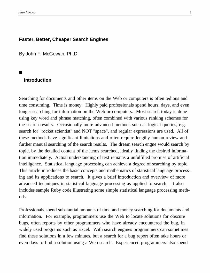
Faster, Better, Cheaper Search Engines

By John F. McGowan, Ph.D.

à

Introduction

Searching for documents and other items on the Web or computers is often tedious andtime consuming. Time is money. Highly paid professionals spend hours, days, and evenlonger searching for information on the Web or computers. Most search today is doneusing key word and phrase matching, often combined with various ranking schemes forthe search results. Occasionally more advanced methods such as logical queries, e.g.search for "rocket scientist" and NOT "space", and regular expressions are used. All ofthese methods have significant limitations and often require lengthy human review andfurther manual searching of the search results. The dream search engne would search bytopic, by the detailed content of the items searched, ideally finding the desired information immediately. Actual understanding of text remains a unfulfilled promise of artificialintelligence. Statistical language processing can achieve a degree of searching by topic.This article introduces the basic concepts and mathematics of statistical language processing and its applications to search. It gives a brief introduction and overview of moreadvanced techniques in statistical language processing as applied to search. It alsoincludes sample Ruby code illustrating some simple statistical language processing methods.

Professionals spend substantial amounts of time and money searching for documents andinformation. For example, programmers use the Web to locate solutions for obscurebugs, often reports by other programmers who have already encountered the bug, inwidely used programs such as Excel. With search engines programmers can sometimesfind these solutions in a few minutes, but a search for a bug report often take hours oreven days to find a solution using a Web search. Experienced programmers also spend

search36.nb 1

hours, even days, relearning how to do things they already know how to do in a newprogramming language, finding out how to use a rarely used feature in a familiar programming language, and identifying undocumented functions. This is often done using thesearch features of online help systems and code editors, often little more than simpleword and phrase matching (or occasionally regular expression matching).

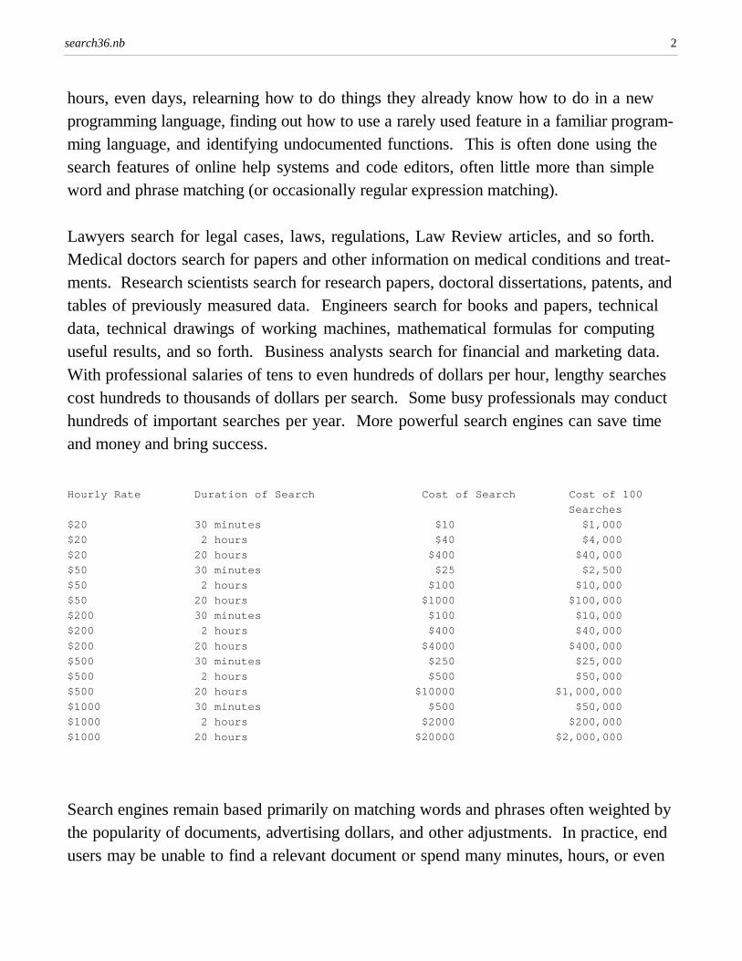
Lawyers search for legal cases, laws, regulations, Law Review articles, and so forth.Medical doctors search for papers and other information on medical conditions and treatments. Research scientists search for research papers, doctoral dissertations, patents, andtables of previously measured data. Engineers search for books and papers, technicaldata, technical drawings of working machines, mathematical formulas for computinguseful results, and so forth. Business analysts search for financial and marketing data.With professional salaries of tens to even hundreds of dollars per hour, lengthy searchescost hundreds to thousands of dollars per search. Some busy professionals may conducthundreds of important searches per year. More powerful search engines can save timeand money and bring success.

Hourly Rate Duration of Search Cost of Search Cost of 100 Searches$20 30 minutes $10 $1,000$20 2 hours $40 $4,000$20 20 hours $400 $40,000$50 30 minutes $25 $2,500$50 2 hours $100 $10,000$50 20 hours $1000 $100,000$200 30 minutes $100 $10,000$200 2 hours $400 $40,000$200 20 hours $4000 $400,000$500 30 minutes $250 $25,000$500 2 hours $500 $50,000$500 20 hours $10000 $1,000,000$1000 30 minutes $500 $50,000$1000 2 hours $2000 $200,000$1000 20 hours $20000 $2,000,000

Search engines remain based primarily on matching words and phrases often weighted bythe popularity of documents, advertising dollars, and other adjustments. In practice, endusers may be unable to find a relevant document or spend many minutes, hours, or even

search36.nb 2

days paging through search results and/or trying many different search words and phrasesin hopes of turning up a relevant document or item. Popularity is not always a good measure of either the relevance or the quality of a document or item. Rankings based onadvertising dollars may not match the needs of the end user of a search engine. Morepowerful methods are needed.

The cause of this costly and frustrating state of search is that present-day search enginescannot understand either the search queries or the documents or items searched. Forexample, if an end user enters the search phrase "rocket scientist", they are probablylooking for information on actual rocket scientists, but not always. Rocket scientist issometimes used as generic term for highly skilled technical professionals in scientific,engineering, and similar fields. A search for "rocket scientist" will occasionally turn uparticles on Wall Street financial engineers, also known as "quants", who are sometimesreferred to as "rocket scientists" in the financial literature. More powerful search engineswill need understanding or a way to emulate some or all aspects of human understanding.

The dream search engine should find documents or other items by topic, not by word orphrase, and return only documents or items related to the topic of interest. Stephen Wolfram's Alpha is being marketed as such a search engine. Time will tell if Alpha is or willbecome the dream search engine. To date, actual understanding of natural language bycomputers has proven extremely difficult, like most problems in artificial intelligence(AI), and successes have been few and limited. Hence, search engines continue to relyon simple word and phrase matching. While actual understanding is probably decades ifnot centuries in the future, statistical language processing methods can achieve a degreeof searching by topic today. Statistical language processing involves measuring and usingthe frequency of words and phrases as well as the absolute and relative positions ofwords and phrases in text.

Closely related problems also occur in recommendation engines and data loss prevention(sometimes identified by the cryptic acronym DLP). Recommendation engines such asNetFlix's Cinematch system, which recommends DVD rentals to customers, recommendpossible purchases based on buying patterns and other data. However, recommendationengines do not understand customer preferences, products, product descriptions, and soforth. Recommendation engines use statistical methods to guess what other products or

search36.nb 3

services customers are likely to purchase, giving the illusion of true understanding.

Data loss prevention consists of systems designed to prevent the accidental or intentionalloss or theft of sensitive information from companies and organizations, for example an e-mail with customer credit card numbers sent to a credit card fraud group overseas. Insome cases, for example social security numbers or credit card numbers, the sensitiveinformation can be identified by matching simple patterns, such as regular expressions.However, some sensitive information, such as a sensitive marketing plan, may lack easilyidentifiable text or numerical patterns. A human being reading the document can identifyit as sensitive easily but a data loss prevention algorithm would fail. Again, even withoutunderstanding, statistical patterns in the text of the document may be able to identify asensitive document.

Reproducing human intelligence on computers, artificial intelligence, has proven baffling.Actual understanding of spoken or written text remains far beyond the state of computerscience. However, statistical language processing can imitate some aspects of humanintelligence and yield more "intelligent" results in speech recognition, machine translation, and search. The rest of this article gives an introduction and overview of the basicconcepts and mathematics of statistical language processing and its applications to improving the speed and lowering the cost of search.

à

A Brief Introduction to Mathematica

This article presents mathematical formulas in the Mathematica programming languageused to compute results and display graphics as well as in standard mathematical notation. Mathematica is an algorithm prototyping and mathematical research tool similar toMatLab. Mathematica and MatLab are scripting language like Python or Ruby withcomprehensive well-integrated mathematical, numerical, and statistical functions. TheMathematica code is retained for greater clarity and detail. The Mathematica code inthis article is usually simple, clear and contains comments in plain English explainingwhat the code does, but may be ignored by those unfamiliar with Mathematica. In addi

search36.nb 4

tion, this article includes sample code in the popular Ruby scripting language. Ruby isfree, open-source software available for Windows, Macintosh, and Unix platforms. Itcan be downloaded from the Ruby web site http://www.ruby-lang.org/.

Technically, everything in Mathematica code is an expression. The key to both understanding Mathematica and the power of Mathematica is a type of expression known as alist. As might be expected, a list is simply a list of elements. A table or matrix in Mathematica is simply a list of lists. Mathematica can represent almost anything as a list.

data = {0,Pi/8,2 Pi/8,3 Pi/8.0,4 Pi/8.0}; (* a simple list in Mathematica, Pi is 3.1415... *)

The mathematical functions that are built into Mathematica are mostly set up to be"listable" so that they act separately on each element of a list.

Sin[data] (* the built in trigonometric sine function in Mathematica is "listable" *)90, SinA π��8 E, 1��è!!!!2 , 0.92388, 1.=

However, some functions are not "listable". Some functions act on a list as a whole.

µ = Mean[data] (* the average or arithmetic mean function is NOT "listable" *)

0.785398

This article uses several functions that act on a list as whole including Length[list],Mean[list], Variance[list], Covariance[list, list], Correlation[list, list], and ListPlot[list].

Most mathematical, numerical, statistical, and graphics functions in Mathematica takelists as arguments and often return lists. The common but flexible list data type enablestight integratiion of the many mathematical functions in Mathematica. Like a set ofLEGO blocks or a TinkerToy, one can quickly create complex mathematical systems as

search36.nb 5

needed.

Mathematica derives from the tradition of list processing languages such as LISP andScheme as well as functional programming that began in the 1960's and has recentlyenjoyed a renaissance. Mathematica has many more advanced list and functional programming features, but for this article and indeed many common tasks the brief introductionabove is all one needs to know.

Mathematica has a forbidding reputation in some circles because it includes extensivesymbolic manipulation capabilities. Mathematica is considered a type of computer algebra system. Some people believe that one must know and use these symbolic capabilitiesto use Mathematica or that Mathematica is only for symbolic manipulation. These symbolic capablities are actually only one subset of Mathematica's capabilities. Mathematicahas the same extensive numerical, statistical, mathematical, and graphics features as Matlab or other competing products (Maple, AXIOM, Maxima, R, and many others).

Mathematica does not require that one use its symbolic capabilities. One can use Mathematica heavily without ever using the symbolic manipulation capabilities. The authorworked on prototypes of image and video processing algorithms at NASA for years without needing to use the symbolic features. The symbolic features are not used in this article. Even quite complex mathematical models of the frequency and location of wordsand phrases in documents that might be developed for search applications would generally not require using the symbolic manipulation features of Mathematica. Mathematicaand Ruby are used for illustration; the needed statistical langugage models can beresearched and developed in many other programming languages.

search36.nb 6

à Correlations

A correlation coefficient is a simple concept from basic statistics. It provides a simplenumerical measure ranging from -1.0 to 1.0 for the correlation betweeen two variables.The main definition of correlation in English is a mutual relationship or connection. Itcan have a more precise meaning: the degree of relative correspondence, as between twosets of data (a correlation of 75 percent). In statistics, a correlation coefficient can beany one of several measures of concommitant variation in two or more variables. In thisarticle and the accompanying sample code, the simplest and most common correlationcoefficient from introductory statistics is used.

The correlation coefficient is built from three simpler concepts in basic statistics: theaverage, the variance, and the covariance. The average of a series of data points is thesum of the values of the data points divided by the number of data points. The average of(0,0,0) is 0. The average of (1,2,3) is 2.

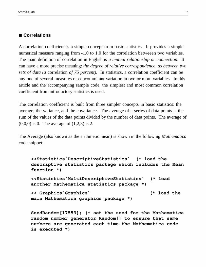
The Average (also known as the arithmetic mean) is shown in the following Mathematicacode snippet:

<<Statistics`DescriptiveStatistics` (* load the descriptive statistics package which includes the Mean function *)

<<Statistics`MultiDescriptiveStatistics` (* load another Mathematica statistics package *)

<< Graphics`Graphics` (* load the main Mathematica graphics package *)

SeedRandom[17553]; (* set the seed for the Mathematica random number generator Random[] to ensure that same numbers are generated each time the Mathematica code is executed *)

search36.nb 7

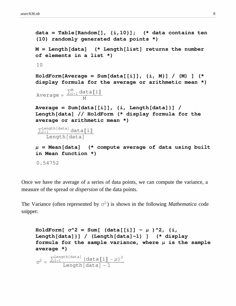
data = Table[Random[], {i,10}]; (* data contains ten (10) randomly generated data points *)

M = Length[data] (* Length[list] returns the number of elements in a list *)

10

HoldForm[Average = Sum[data[[i]], {i, M}] / (M) ] (* display formula for the average or arithmetic mean *)

Average = ⁄i=1M dataPiT��M

Average = Sum[data[[i]], {i, Length[data]}] / Length[data] // HoldForm (* display formula for the average or arithmetic mean *)⁄i=1

Length@dataD dataPiT��Length@dataDµ = Mean[data] (* compute average of data using built in Mean function *)

0.54752

Once we have the average of a series of data points, we can compute the variance, ameasure of the spread or dispersion of the data points.

The Variance (often represented by σ2 ) is shown in the following Mathematica codesnippet:

HoldForm[ σ^2 = Sum[ (data[[i]] - µ )^2, {i, Length[data]}] / (Length[data]-1) ] (* display formula for the sample variance, where µ is the sample average *)

σ2 = ⁄i=1Length@dataD HdataPiT − µL2

��Length@dataD − 1

search36.nb 8

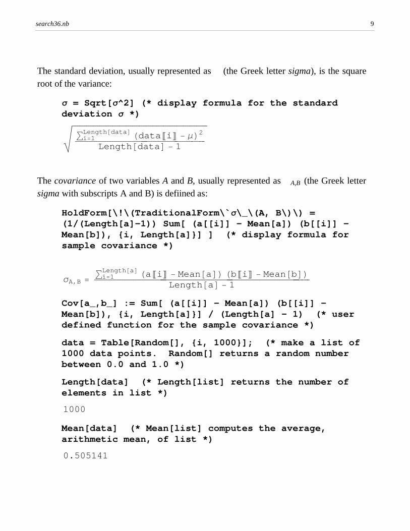
The standard deviation, usually represented as s (the Greek letter sigma), is the squareroot of the variance:

σ = Sqrt[σ^2] (* display formula for the standard deviation σ *)

$%%%%%%%%%%%%%%%%%%%%%%%%%%%%%%%%%%%%%%%%%%%%%%%%%%%%%%%%%%%%%⁄i=1Length@dataD HdataPiT − µL2

��Length@dataD − 1

The covariance of two variables A and B, usually represented as sA,B (the Greek lettersigma with subscripts A and B) is defiined as:

HoldForm[\!$TraditionalForm\`σ\_\(A, B$\) = (1/(Length[a]-1)) Sum[ (a[[i]] - Mean[a]) (b[[i]] - Mean[b]), {i, Length[a]}] ] (* display formula for sample covariance *)

σA,B = ⁄i=1Length@aD HaPiT − Mean@aDL HbPiT − Mean@bDL��Length@aD − 1

Cov[a_,b_] := Sum[ (a[[i]] - Mean[a]) (b[[i]] - Mean[b]), {i, Length[a]}] / (Length[a] - 1) (* user defined function for the sample covariance *)

data = Table[Random[], {i, 1000}]; (* make a list of 1000 data points. Random[] returns a random number between 0.0 and 1.0 *)

Length[data] (* Length[list] returns the number of elements in list *)

1000

Mean[data] (* Mean[list] computes the average, arithmetic mean, of list *)

0.505141

search36.nb 9

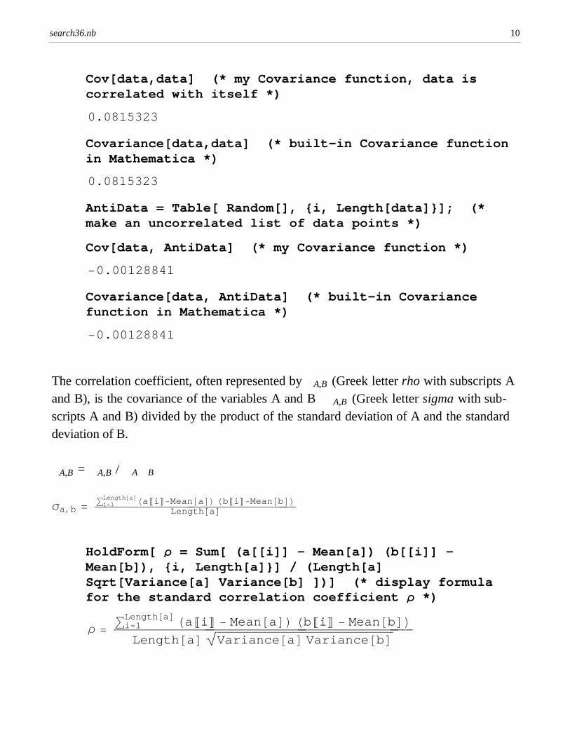
Cov[data,data] (* my Covariance function, data is correlated with itself *)

0.0815323

Covariance[data,data] (* built-in Covariance function in Mathematica *)

0.0815323

AntiData = Table[ Random[], {i, Length[data]}]; (* make an uncorrelated list of data points *)

Cov[data, AntiData] (* my Covariance function *)

−0.00128841

Covariance[data, AntiData] (* built-in Covariance function in Mathematica *)

−0.00128841

The correlation coefficient, often represented by rA,B (Greek letter rho with subscripts Aand B), is the covariance of the variables A and B sA,B (Greek letter sigma with subscripts A and B) divided by the product of the standard deviation of A and the standarddeviation of B.

rA,B = sA,B / sA sB

σa,b = ⁄i=1Length@aDHaPiT−Mean@aDL HbPiT−Mean@bDL��Length@aD

HoldForm[ ρ = Sum[ (a[[i]] - Mean[a]) (b[[i]] - Mean[b]), {i, Length[a]}] / (Length[a] Sqrt[Variance[a] Variance[b] ])] (* display formula for the standard correlation coefficient ρ *)

ρ = ⁄i=1Length@aD HaPiT − Mean@aDL HbPiT − Mean@bDL��Length@aD è!!!!!!!!!!!!!!!!!!!!!!!!!!!!!!!!!!!!!!!!!!!!!!!!!!!!!!!!!!Variance@aD Variance@bD

search36.nb 10

Corr[a_,b_] := Sum[ (a[[i]] - Mean[a]) (b[[i]] - Mean[b]), {i, Length[a]}] / ((Length[a]-1) Sqrt[Variance[a] Variance[b] ]) (* end user defined correlation coefficient function *)

Corr[data, data] (* my Correlation function, defined above *)

1.

Correlation[data,data] (* built in Mathematica Correlation function *)

1.

Corr[data, AntiData] (* correlation calculated using the user defined function Corr *)

−0.0156761

Correlation[data, AntiData] (* correlation calculated using the built in Mathematica function *)

−0.0156761

ü The Limits of Correlation Coefficients

The standard correlation coefficient only works well for linear relationships. In the example below the random variables X and Y are closely related by the equation Y = Sin(X), anon-linear relationship. However, the expectation value of the standard correlation coefficient in the example below is 0.0. The variables appear unrelated if the standard correlation coefficient is used. The expectation value of a discrete random variable X is ⁄ xP(x) where x is the value of X and P(x) is the probability of that value. For example,consider flipping a fair coin. If one gives the value 1.0 to heads and -1.0 to tails, theexpectation value of the coin flip is 0.0 = 0.5*1.0 + 0.5*(-1.0).

search36.nb 11

X = Table[ Pi Random[], {i, 1000}]; (* make list of data ranging from 0.0 to π (3.1415...) *)Y = Sin[X]; (* make list of data Y where each element is the sine function of the corresponding element in the list X *)

Correlation[X, X] (* the correlation of a data sample with itself is 1.0 *)

1.

Correlation[X, 2 X] (* the correlation of a data sample with 2.0 times itself is 1.0 *)

1.

Correlation[X, -X] (* the correlation of a data sample with -1.0 times itself is 1.0 *)

−1.

Correlation[X, -2 X] (* the correlation of a data sample with -2.0 times itself is 1.0 *)

−1.

The variables X and Y are essentially uncorrelated as measured by the standard correlation coefficient. The standard correlation coefficient is almost zero. In fact, the expectation value of the correlation coefficient is exactly zero in this example.

Correlation[X,Y] (* the correlation between a data sample X and Y = Sin[X] is zero *)

−0.00465432

However, the variables X and Y are actually closely related because Y = Sin(X), a non-linear relationship that is not detected by the correlation coefficient:

search36.nb 12

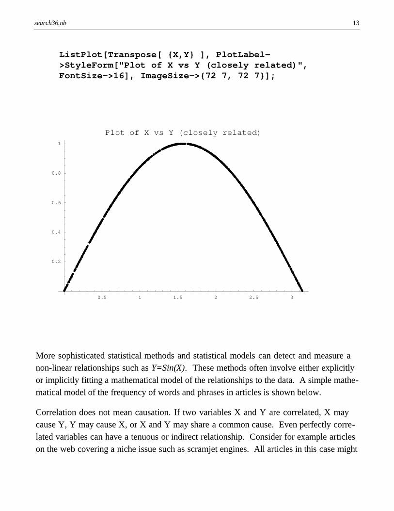
ListPlot[Transpose[ {X,Y} ], PlotLabel->StyleForm["Plot of X vs Y (closely related)", FontSize->16], ImageSize->{72 7, 72 7}];

0.5 1 1.5 2 2.5 3

0.2

0.4

0.6

0.8

1

Plot of X vs Y Hclosely relatedL

More sophisticated statistical methods and statistical models can detect and measure anon-linear relationships such as Y=Sin(X). These methods often involve either explicitlyor implicitly fitting a mathematical model of the relationships to the data. A simple mathematical model of the frequency of words and phrases in articles is shown below.

Correlation does not mean causation. If two variables X and Y are correlated, X maycause Y, Y may cause X, or X and Y may share a common cause. Even perfectly correlated variables can have a tenuous or indirect relationship. Consider for example articleson the web covering a niche issue such as scramjet engines. All articles in this case might

search36.nb 13

be written by one aerospace journalist, say "Karman Von Theodore", All articles onscramjets would be perfectly correlated with "Karman Von Theodore" but the correlationwould be quite tenuous. If "Karman Von Theodore" retired or ceased writing articles onscramjet engines, the correlation would suddently disappear. It requires more than acorrelation to determine the nature of the relationship between two or more variables.

à N-Grams

An N-Gram is a simple concept used in speech recognition, machine translation, andlanguage processing. A 1-gram or unigram is simply a single word such as "the" or"rocket". A 2-gram or bigram is simply a pair of adjacent words such as "ice cream" or"I scream". A 3-gram or trigram is simply three adjacent words such as "ice cream cone"or "I scream loudly". An N-gram is simply N adjacent words where N is any integer(1,2,3,...).

Standard Hidden Markov Model (HMM) based speech recognition algorithms makeheavy use of N-Grams, often trigrams, to recognize speech. Even if speech recognitionalgorithms could recognize the sounds in speech, the so-called phonemes such as the"AH" sound in "father", as well as human beings, speech contains homonyms and near-homonyms such as "I scream" and "ice cream" that cannot be distinguished by soundalone. Human beings resolve homonyms and near-homonyms by actually understandingthe speech and determining the correct words from context. Computer programs are along way from actual understanding of language. However, speech recognition algorithms can use statistical models of the frequency of N-grams to determine what was said.For example, consider the trigrams "I scream loudly" and "ice cream cone". People areless likely to say "I scream cone" or "ice cream loudly" than "I scream loudly" or "icecream cone". The words "loudly" and "cone" are not homonyms or near homonyms.They are acoustically distinctive. Thus, a speech recognition algorithm can use the frequency of trigrams such as "I scream loudly" and "ice cream cone" to successsfullyresolve "I scream" and "ice cream".

Current HMM speech recognition algorithms use statistical language models of the fre

search36.nb 14

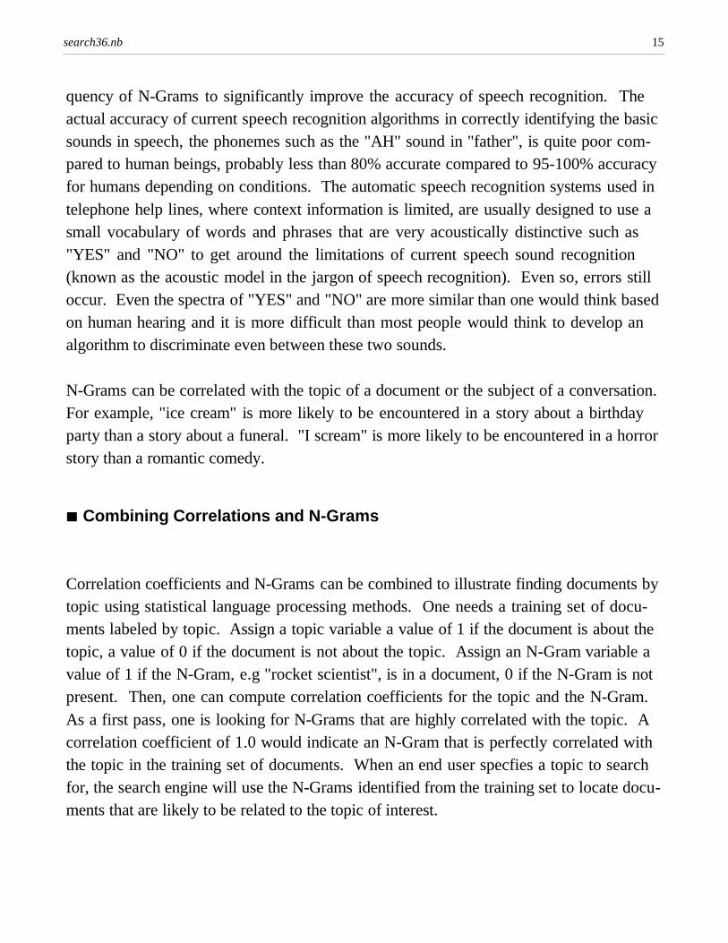
quency of N-Grams to significantly improve the accuracy of speech recognition. Theactual accuracy of current speech recognition algorithms in correctly identifying the basicsounds in speech, the phonemes such as the "AH" sound in "father", is quite poor compared to human beings, probably less than 80% accurate compared to 95-100% accuracyfor humans depending on conditions. The automatic speech recognition systems used intelephone help lines, where context information is limited, are usually designed to use asmall vocabulary of words and phrases that are very acoustically distinctive such as"YES" and "NO" to get around the limitations of current speech sound recognition(known as the acoustic model in the jargon of speech recognition). Even so, errors stilloccur. Even the spectra of "YES" and "NO" are more similar than one would think basedon human hearing and it is more difficult than most people would think to develop analgorithm to discriminate even between these two sounds.

N-Grams can be correlated with the topic of a document or the subject of a conversation.For example, "ice cream" is more likely to be encountered in a story about a birthdayparty than a story about a funeral. "I scream" is more likely to be encountered in a horrorstory than a romantic comedy.

à Combining Correlations and N-Grams

Correlation coefficients and N-Grams can be combined to illustrate finding documents bytopic using statistical language processing methods. One needs a training set of documents labeled by topic. Assign a topic variable a value of 1 if the document is about thetopic, a value of 0 if the document is not about the topic. Assign an N-Gram variable avalue of 1 if the N-Gram, e.g "rocket scientist", is in a document, 0 if the N-Gram is notpresent. Then, one can compute correlation coefficients for the topic and the N-Gram.As a first pass, one is looking for N-Grams that are highly correlated with the topic. Acorrelation coefficient of 1.0 would indicate an N-Gram that is perfectly correlated withthe topic in the training set of documents. When an end user specfies a topic to searchfor, the search engine will use the N-Grams identified from the training set to locate documents that are likely to be related to the topic of interest.

search36.nb 15

à Example Ruby Code

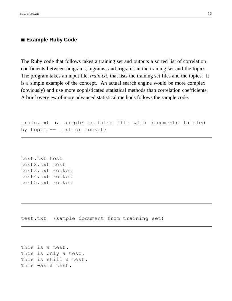
The Ruby code that follows takes a training set and outputs a sorted list of correlationcoefficients between unigrams, bigrams, and trigrams in the training set and the topics.The program takes an input file, train.txt, that lists the training set files and the topics. Itis a simple example of the concept. An actual search engine would be more complex(obviously) and use more sophisticated statistical methods than correlation coefficients.A brief overview of more advanced statistical methods follows the sample code.

train.txt (a sample training file with documents labeledby topic -- test or rocket)

test.txt testtest2.txt testtest3.txt rockettest4.txt rockettest5.txt rocket

test.txt (sample document from training set)

This is a test.This is only a test.This is still a test.This was a test.

search36.nb 16

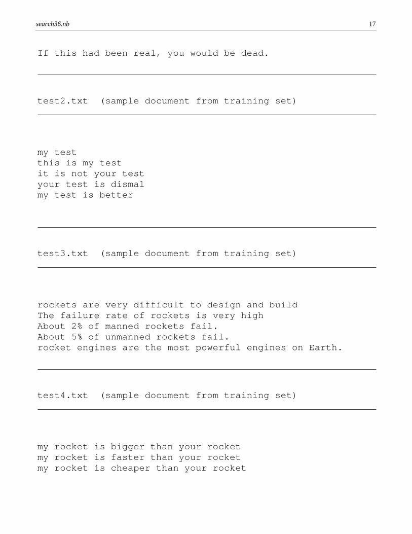
If this had been real, you would be dead.

test2.txt (sample document from training set)

my testthis is my testit is not your testyour test is dismalmy test is better


rockets are very difficult to design and buildThe failure rate of rockets is very highAbout 2% of manned rockets fail.About 5% of unmanned rockets fail.rocket engines are the most powerful engines on Earth.


my rocket is bigger than your rocketmy rocket is faster than your rocketmy rocket is cheaper than your rocket

search36.nb 17

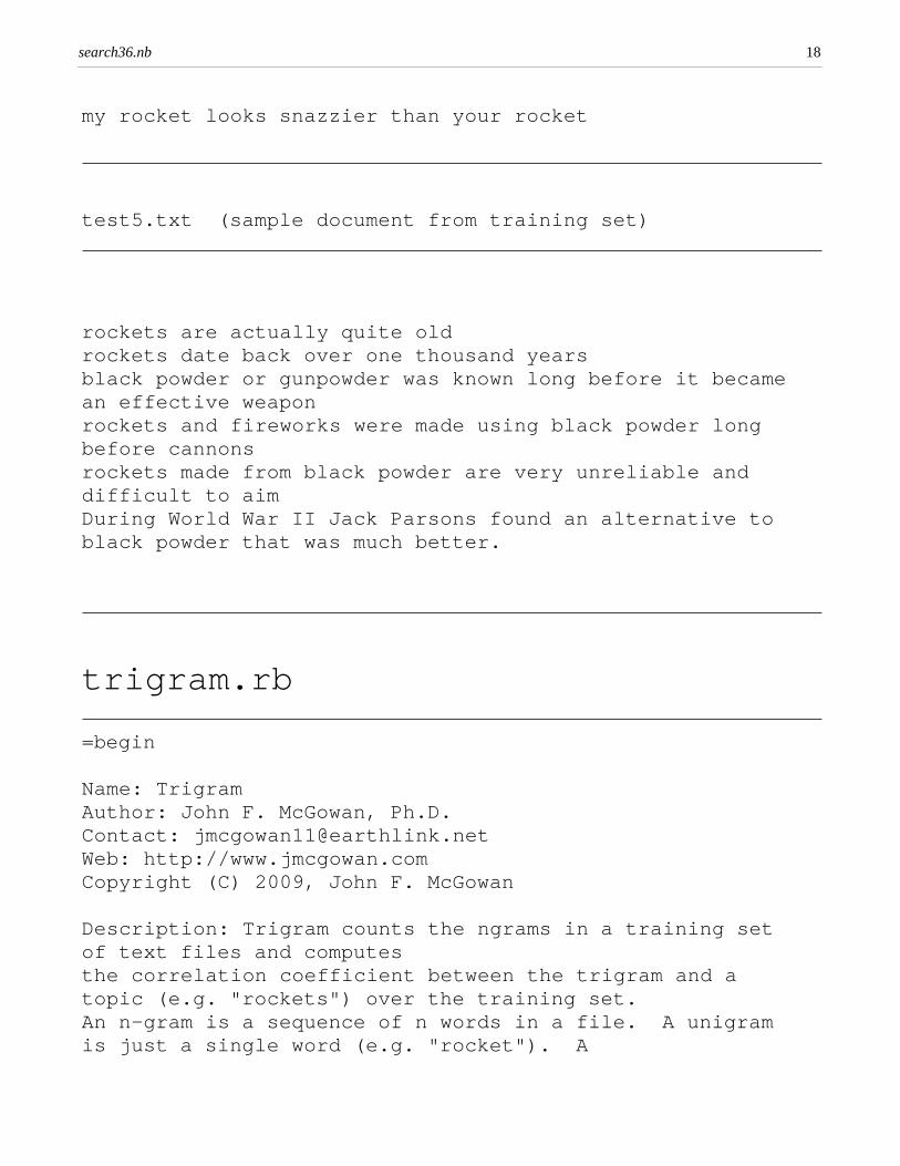
my rocket looks snazzier than your rocket


rockets are actually quite oldrockets date back over one thousand yearsblack powder or gunpowder was known long before it became an effective weaponrockets and fireworks were made using black powder long before cannonsrockets made from black powder are very unreliable and difficult to aimDuring World War II Jack Parsons found an alternative to black powder that was much better.

trigram.rb

=begin

Name: TrigramAuthor: John F. McGowan, Ph.D.Contact: [email protected]: http://www.jmcgowan.comCopyright (C) 2009, John F. McGowan

Description: Trigram counts the ngrams in a training set of text files and computesthe correlation coefficient between the trigram and a topic (e.g. "rockets") over the training set.An n-gram is a sequence of n words in a file. A unigram is just a single word (e.g. "rocket"). A

search36.nb 18

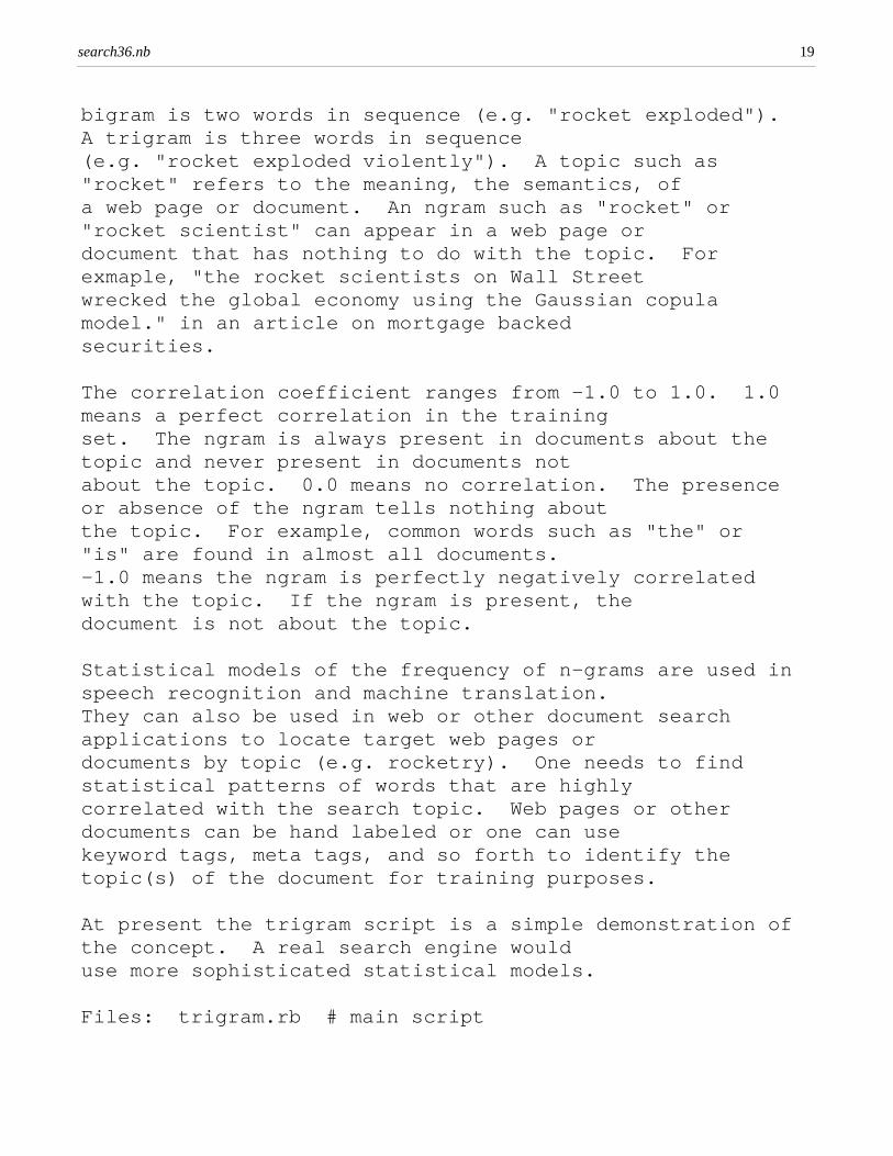
bigram is two words in sequence (e.g. "rocket exploded"). A trigram is three words in sequence(e.g. "rocket exploded violently"). A topic such as "rocket" refers to the meaning, the semantics, of a web page or document. An ngram such as "rocket" or "rocket scientist" can appear in a web page ordocument that has nothing to do with the topic. For exmaple, "the rocket scientists on Wall Streetwrecked the global economy using the Gaussian copula model." in an article on mortgage backedsecurities.

The correlation coefficient ranges from -1.0 to 1.0. 1.0 means a perfect correlation in the trainingset. The ngram is always present in documents about the topic and never present in documents notabout the topic. 0.0 means no correlation. The presence or absence of the ngram tells nothing aboutthe topic. For example, common words such as "the" or "is" are found in almost all documents.-1.0 means the ngram is perfectly negatively correlated with the topic. If the ngram is present, thedocument is not about the topic.

Statistical models of the frequency of n-grams are used in speech recognition and machine translation. They can also be used in web or other document search applications to locate target web pages or documents by topic (e.g. rocketry). One needs to find statistical patterns of words that are highlycorrelated with the search topic. Web pages or other documents can be hand labeled or one can usekeyword tags, meta tags, and so forth to identify the topic(s) of the document for training purposes.

At present the trigram script is a simple demonstration of the concept. A real search engine would use more sophisticated statistical models.

Files: trigram.rb # main script

search36.nb 19

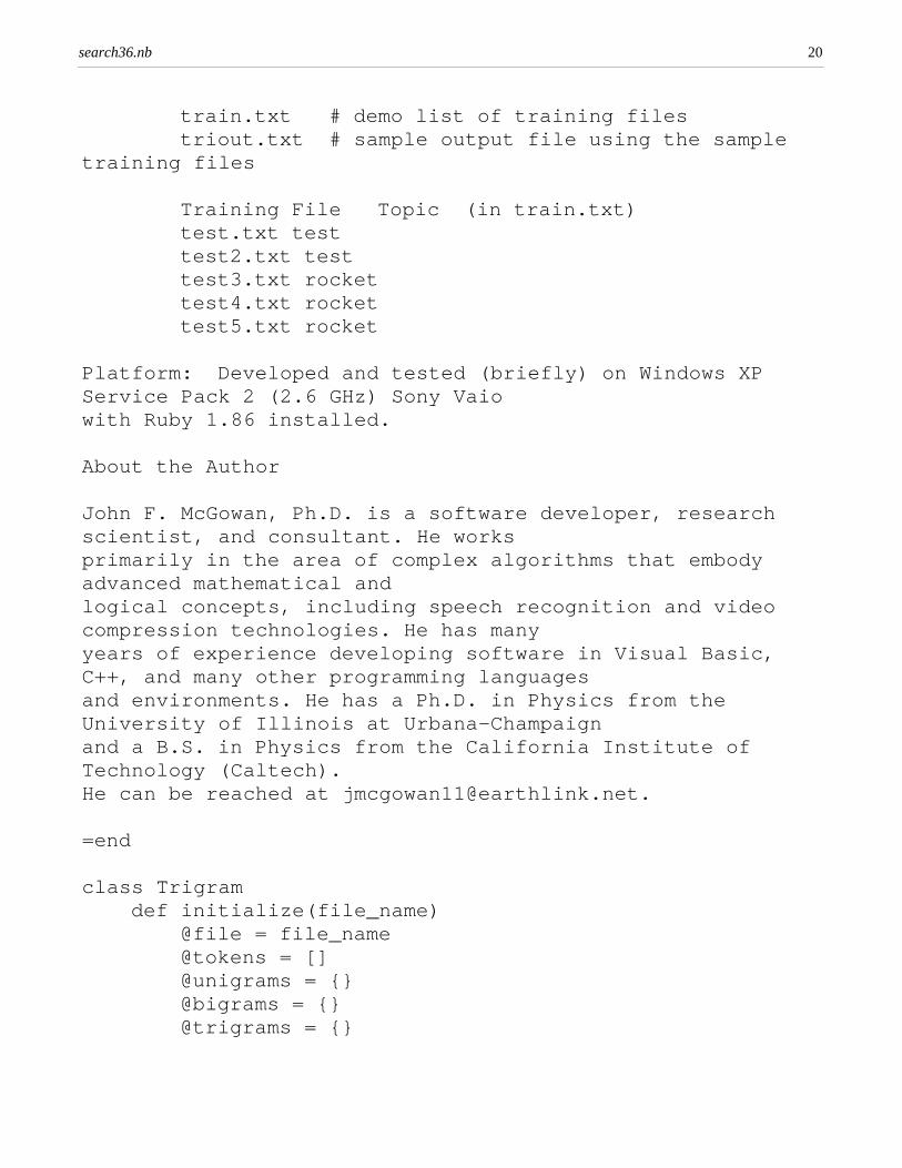
train.txt # demo list of training filestriout.txt # sample output file using the sample

training files

Training File Topic (in train.txt)test.txt testtest2.txt testtest3.txt rockettest4.txt rockettest5.txt rocket

Platform: Developed and tested (briefly) on Windows XP Service Pack 2 (2.6 GHz) Sony Vaio with Ruby 1.86 installed.

About the Author

John F. McGowan, Ph.D. is a software developer, research scientist, and consultant. He works primarily in the area of complex algorithms that embody advanced mathematical and logical concepts, including speech recognition and video compression technologies. He has many years of experience developing software in Visual Basic, C++, and many other programming languages and environments. He has a Ph.D. in Physics from the University of Illinois at Urbana-Champaign and a B.S. in Physics from the California Institute of Technology (Caltech). He can be reached at [email protected].

=end

class Trigramdef initialize(file_name)

@file = file_name@tokens = []@unigrams = {}@bigrams = {}@trigrams = {}

search36.nb 20

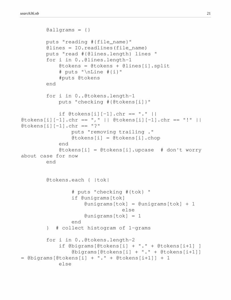
@allgrams = {}

puts "reading #{file_name}"@lines = IO.readlines(file_name)puts "read #{@lines.length} lines "for i in [email protected]

@tokens = @tokens + @lines[i].split# puts "\nLine #{i}"#puts @tokens

end

for i in [email protected] "checking #{@tokens[i]}"

if @tokens[i][-1].chr == "." || @tokens[i][-1].chr == "," || @tokens[i][-1].chr == "!" || @tokens[i][-1].chr == "?"

puts "removing trailing ."@tokens[i] = @tokens[i].chop

end@tokens[i] = @tokens[i].upcase # don't worry

about case for nowend

@tokens.each { |tok|

# puts "checking #{tok} "if @unigrams[tok]

@unigrams[tok] = @unigrams[tok] + 1 else

@unigrams[tok] = 1end

} # collect histogram of 1-grams

for i in [email protected] @bigrams[@tokens[i] + "." + @tokens[i+1] ]

@bigrams[@tokens[i] + "." + @tokens[i+1]] = @bigrams[@tokens[i] + "." + @tokens[i+1]] + 1

else

search36.nb 21

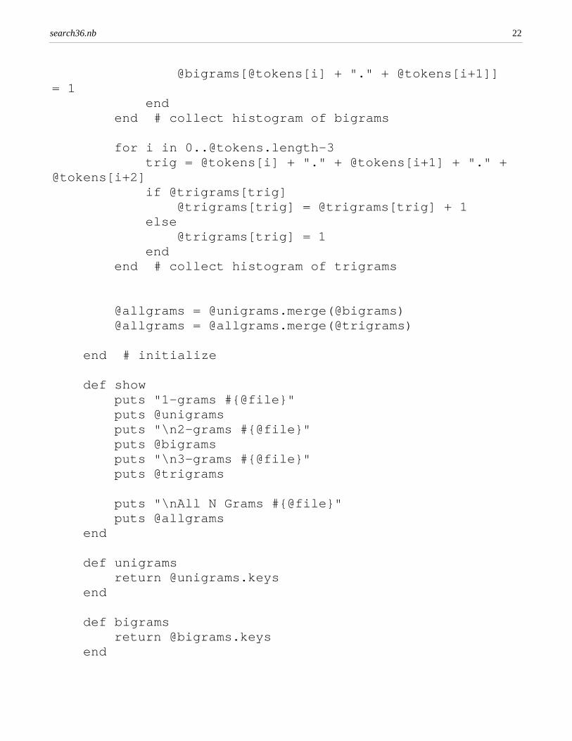
@bigrams[@tokens[i] + "." + @tokens[i+1]] = 1

endend # collect histogram of bigrams

for i in [email protected] = @tokens[i] + "." + @tokens[i+1] + "." +

@tokens[i+2]if @trigrams[trig]

@trigrams[trig] = @trigrams[trig] + 1else

@trigrams[trig] = 1end

end # collect histogram of trigrams

@allgrams = @unigrams.merge(@bigrams)@allgrams = @allgrams.merge(@trigrams)

end # initialize

def showputs "1-grams #{@file}"puts @unigramsputs "\n2-grams #{@file}"puts @bigramsputs "\n3-grams #{@file}"puts @trigrams

puts "\nAll N Grams #{@file}"puts @allgrams

end

def unigramsreturn @unigrams.keys

end

def bigramsreturn @bigrams.keys

end

search36.nb 22

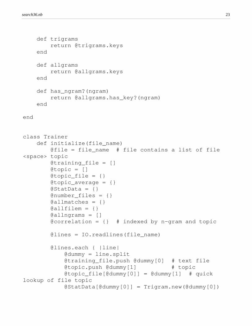
def trigramsreturn @trigrams.keys

end

def allgramsreturn @allgrams.keys

end

def has_ngram?(ngram)return @allgrams.has_key?(ngram)

end

end

class Trainerdef initialize(file_name)

@file = file_name # file contains a list of file <space> topic

@training_file = []@topic = []@topic_file = {}@topic_average = {}@StatData = {}@number_files = {}@allmatches = {}@allfilem = {}@allngrams = [] @correlation = {} # indexed by n-gram and topic

@lines = IO.readlines(file_name)

@lines.each { |line|@dummy = line.split@training_file.push @dummy[0] # text [email protected] @dummy[1] # topic@topic_file[@dummy[0]] = @dummy[1] # quick

lookup of file topic@StatData[@dummy[0]] = Trigram.new(@dummy[0])

search36.nb 23

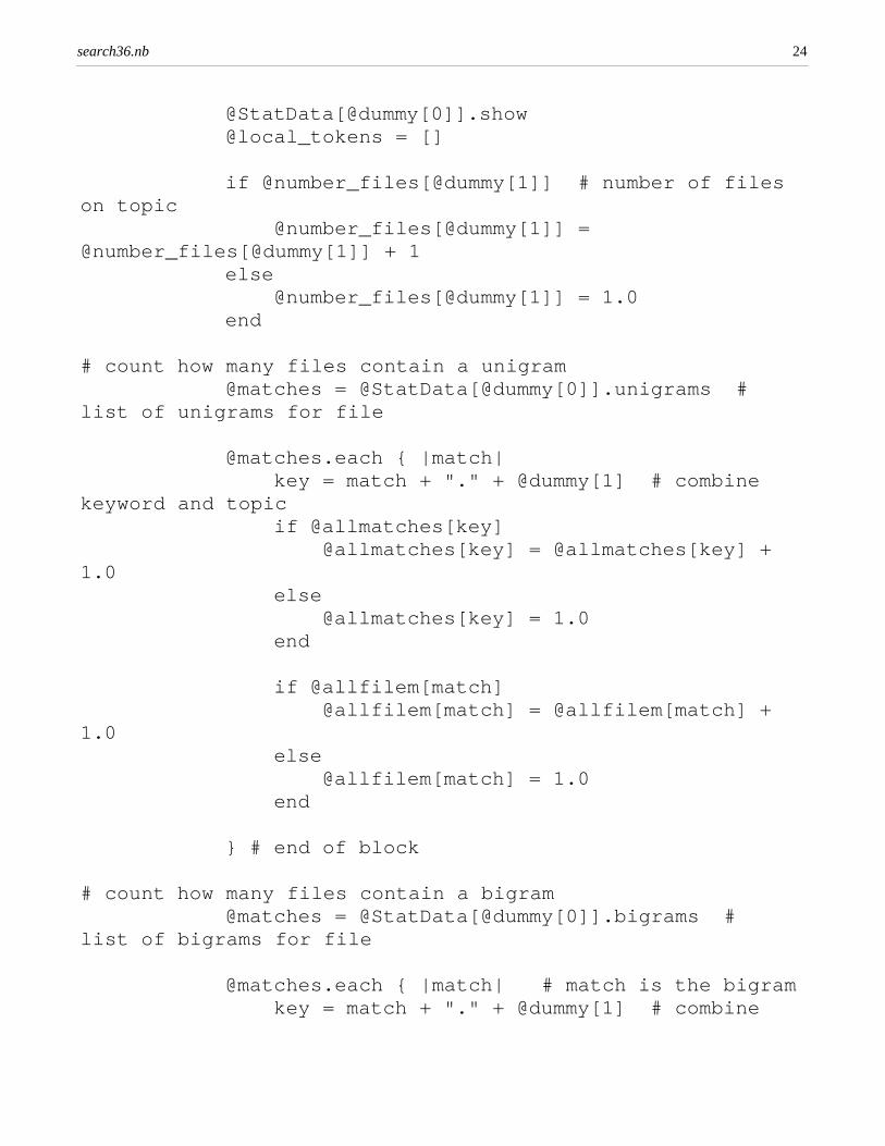
@StatData[@dummy[0]].show@local_tokens = []

if @number_files[@dummy[1]] # number of files on topic

@number_files[@dummy[1]] = @number_files[@dummy[1]] + 1

else@number_files[@dummy[1]] = 1.0

end

# count how many files contain a unigram@matches = @StatData[@dummy[0]].unigrams #

list of unigrams for file

@matches.each { |match|key = match + "." + @dummy[1] # combine

keyword and topicif @allmatches[key]

@allmatches[key] = @allmatches[key] + 1.0

else@allmatches[key] = 1.0

end

if @allfilem[match]@allfilem[match] = @allfilem[match] +

1.0else

@allfilem[match] = 1.0end

} # end of block

# count how many files contain a bigram@matches = @StatData[@dummy[0]].bigrams #

list of bigrams for file

@matches.each { |match| # match is the bigramkey = match + "." + @dummy[1] # combine

search36.nb 24

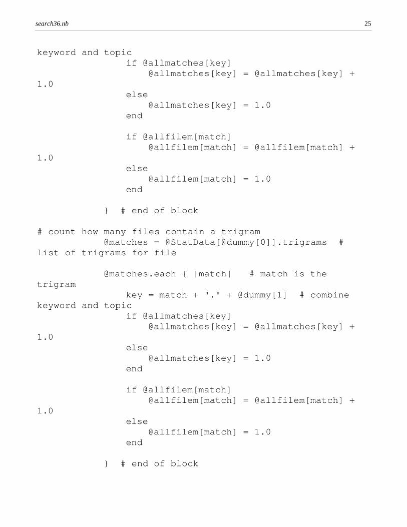
keyword and topicif @allmatches[key]

@allmatches[key] = @allmatches[key] + 1.0

else@allmatches[key] = 1.0

end


1.0else


} # end of block

# count how many files contain a trigram@matches = @StatData[@dummy[0]].trigrams #

list of trigrams for file

@matches.each { |match| # match is the trigram

key = match + "." + @dummy[1] # combine keyword and topic

if @allmatches[key] @allmatches[key] = @allmatches[key] +

1.0else

@allmatches[key] = 1.0end


1.0else


} # end of block

search36.nb 25

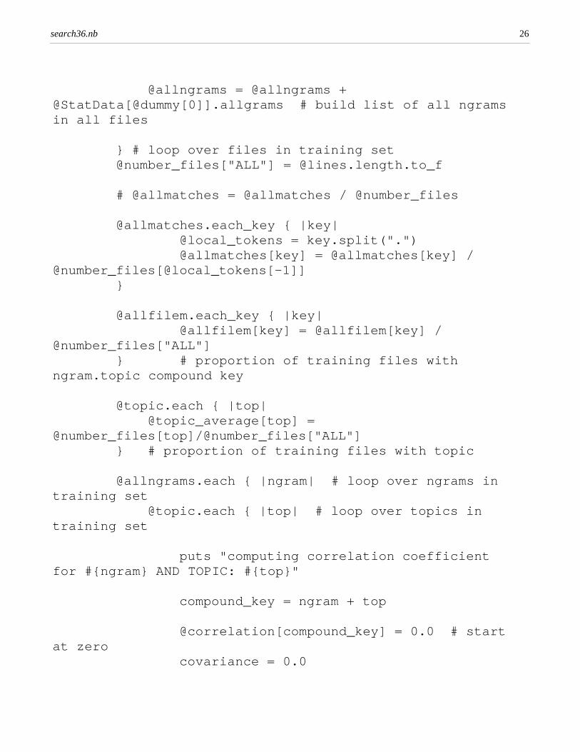
@allngrams = @allngrams + @StatData[@dummy[0]].allgrams # build list of all ngrams in all files

} # loop over files in training set@number_files["ALL"] = @lines.length.to_f

# @allmatches = @allmatches / @number_files

@allmatches.each_key { |key|@local_tokens = key.split(".")@allmatches[key] = @allmatches[key] /

@number_files[@local_tokens[-1]]}

@allfilem.each_key { |key|@allfilem[key] = @allfilem[key] /

@number_files["ALL"]} # proportion of training files with

ngram.topic compound key

@topic.each { |top|@topic_average[top] =

@number_files[top]/@number_files["ALL"]} # proportion of training files with topic

@allngrams.each { |ngram| # loop over ngrams in training set

@topic.each { |top| # loop over topics in training set

puts "computing correlation coefficient for #{ngram} AND TOPIC: #{top}"

compound_key = ngram + top

@correlation[compound_key] = 0.0 # start at zero

covariance = 0.0

search36.nb 26

variance_ngram = 0.0variance_topic = 0.0

# @correlation[ngram.topic] = covariance/Math.sqrt(variance_ngram*variance_topic)

@training_file.each { |file|if @topic_file[file] == top

delta_top = (1.0 - @topic_average[top])

elsedelta_top = (0.0 -

@topic_average[top])end

variance_topic = variance_topic + delta_top**2

if @StatData[file].has_ngram?(ngram)delta_ngram = (1.0 -

@allfilem[ngram])else

delta_ngram = (0.0 - @allfilem[ngram])

endvariance_ngram = variance_ngram +

delta_ngram**2

covariance = covariance + delta_top*delta_ngram

} # loop over files in training set

@correlation[compound_key] = covariance/ Math.sqrt(variance_ngram*variance_topic)

}}

end

search36.nb 27

def showputs "\nTraining Files"puts @training_fileputs "\nTopics"puts @topic

puts @StatData

puts "\nUnigram Match Statistics"sorted = @allmatches.sort {|a,b| a[1]<=>b[1]} #

sort result by value (not key) sorted.each { |match| puts match }puts "\nUnigram Statistics over All Files"sorted = @allfilem.sort {|a,b| a[1] <=> b[1]} #

sort by valuesorted.each { |match| puts match }

puts "\nTopic Average"puts @topic_average

puts "\nCorrelations"sorted = @correlation.sort {|a,b| a[1] <=> b[1]}

# sort by valuesorted.each { |match| puts match }

end end

# simple demo

#t = Trigram.new("test.txt")

#t.show

set = Trainer.new("train.txt")

set.show

search36.nb 28

à Advanced Statistical Models of Text

An advanced search engine searches by topic not by direct key word or phrase matching.For example, one end user might search for articles on the topic "Wall Street", meanngthe financial industry, not the exact phrase "Wall Street". Another end user might searchfor articles on the topic "NASA," the National Aeronautics and Space Administration.Instead of searching for the phrase "Wall Street" or "NASA", an advanced search enginesearches for statistical patterns of words and phrases that occur when the topic "WallStreet" or "NASA" is discussed. For example, both "space" and "rocket scientist" tend tooccur in articles about NASA. However, the phrase "rocket scientist" also occurs inarticles about so-called financial engineering on Wall Street (meaning in the financialindustry). In general, an advanced search engine needs sophisticated statistical models ofthe frequency and/or location of words and phrases in a document as a function of topic.

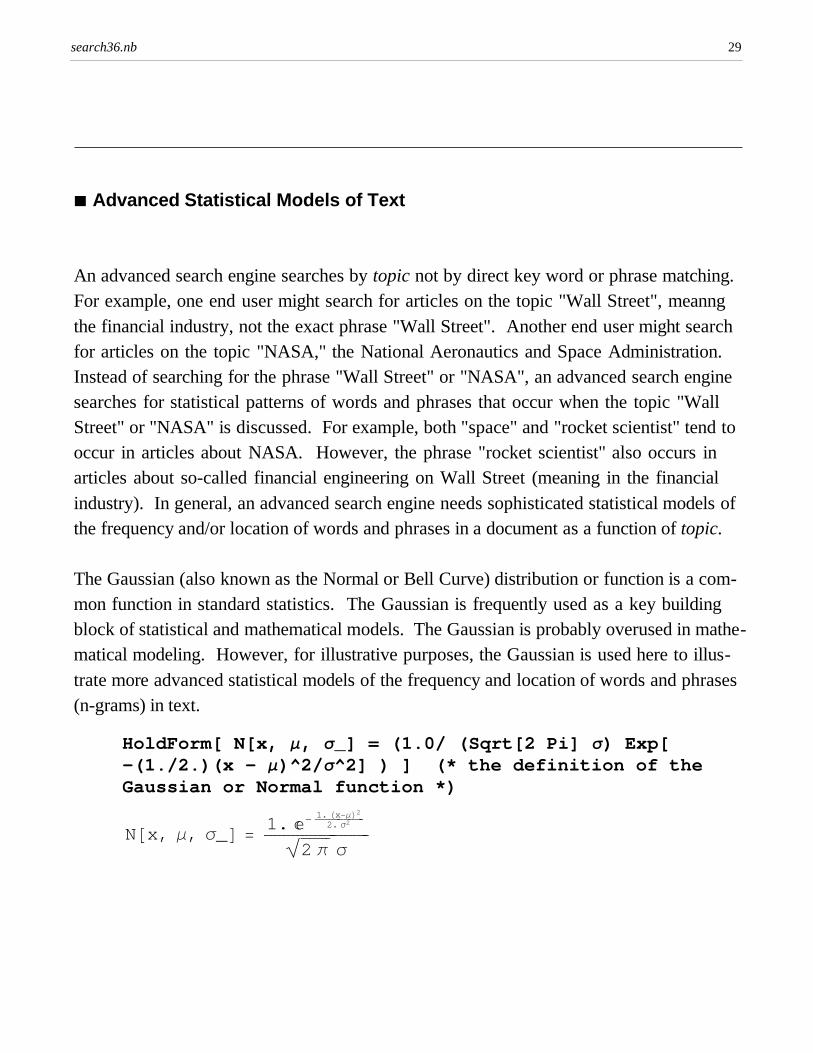
The Gaussian (also known as the Normal or Bell Curve) distribution or function is a common function in standard statistics. The Gaussian is frequently used as a key buildingblock of statistical and mathematical models. The Gaussian is probably overused in mathematical modeling. However, for illustrative purposes, the Gaussian is used here to illustrate more advanced statistical models of the frequency and location of words and phrases(n-grams) in text.

HoldForm[ N[x, µ, σ_] = (1.0/ (Sqrt[2 Pi] σ) Exp[ -(1./2.)(x - µ)^2/σ^2] ) ] (* the definition of the Gaussian or Normal function *)

N@x, µ, σ_D = 1. ã− 1. Hx−µL2��2. σ2

��è!!!!!!!2 π σ

search36.nb 29

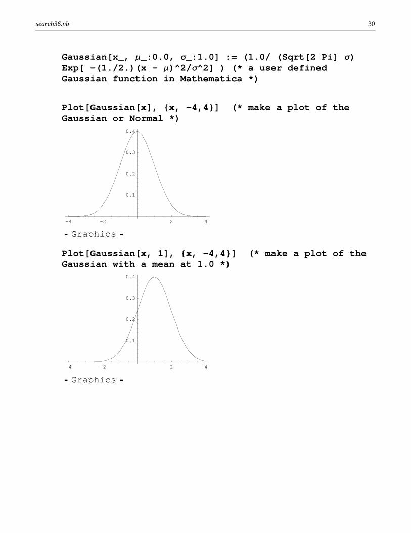
Gaussian[x_, µ_:0.0, σ_:1.0] := (1.0/ (Sqrt[2 Pi] σ) Exp[ -(1./2.)(x - µ)^2/σ^2] ) (* a user defined Gaussian function in Mathematica *)

Plot[Gaussian[x], {x, -4,4}] (* make a plot of the Gaussian or Normal *)

-4 -2 2 4

0.1

0.2

0.3

0.4

� Graphics �

Plot[Gaussian[x, 1], {x, -4,4}] (* make a plot of the Gaussian with a mean at 1.0 *)

-4 -2 2 4

0.1

0.2

0.3

0.4

� Graphics �

search36.nb 30

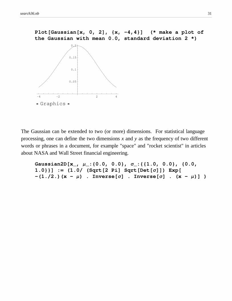
Plot[Gaussian[x, 0, 2], {x, -4,4}] (* make a plot of the Gaussian with mean 0.0, standard deviation 2 *)

-4 -2 2 4

0.05

0.1

0.15

0.2

� Graphics �

The Gaussian can be extended to two (or more) dimensions. For statistical languageprocessing, one can define the two dimensions x and y as the frequency of two differentwords or phrases in a document, for example "space" and "rocket scientist" in articlesabout NASA and Wall Street financial engineering.

Gaussian2D[x_, µ_:{0.0, 0.0}, σ_:{{1.0, 0.0}, {0.0, 1.0}}] := (1.0/ (Sqrt[2 Pi] Sqrt[Det[σ]]) Exp[ -(1./2.)(x - µ) . Inverse[σ] . Inverse[σ] . (x - µ)] )

search36.nb 31

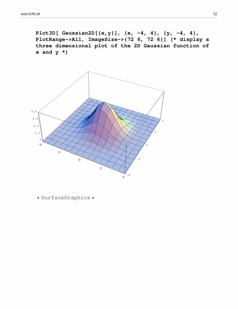
Plot3D[ Gaussian2D[{x,y}], {x, -4, 4}, {y, -4, 4}, PlotRange->All, ImageSize->{72 6, 72 6}] (* display a three dimensional plot of the 2D Gaussian function of x and y *)

-4

-2

0

2

4 -4

-2

0

2

4

0

0.1

0.2

0.3

0.4

-4

-2

0

2

4

� SurfaceGraphics �

search36.nb 32

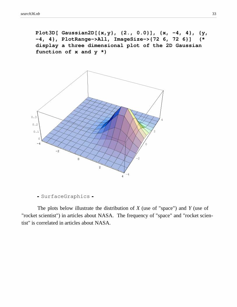
Plot3D[ Gaussian2D[{x,y}, {2., 0.0}], {x, -4, 4}, {y, -4, 4}, PlotRange->All, ImageSize->{72 6, 72 6}] (* display a three dimensional plot of the 2D Gaussian function of x and y *)

-4

-2

0

2

4 -4

-2

0

2

4

0

0.1

0.2

0.3

-4

-2

0

2

4


The plots below illustrate the distribution of X (use of "space") and Y (use of"rocket scientist") in articles about NASA. The frequency of "space" and "rocket scientist" is correlated in articles about NASA.

search36.nb 33

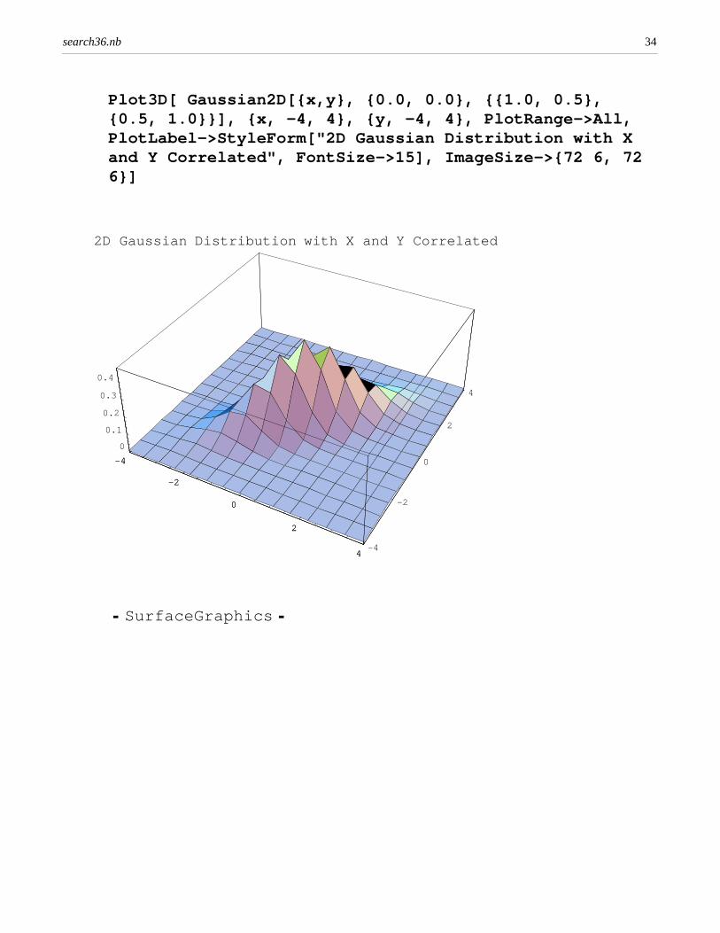
Plot3D[ Gaussian2D[{x,y}, {0.0, 0.0}, {{1.0, 0.5}, {0.5, 1.0}}], {x, -4, 4}, {y, -4, 4}, PlotRange->All, PlotLabel->StyleForm["2D Gaussian Distribution with X and Y Correlated", FontSize->15], ImageSize->{72 6, 72 6}]

2D Gaussian Distribution with X and Y Correlated

-4

-2

0

2

4 -4

-2

0

2

4

0

0.1

0.2

0.3

0.4

-4

-2

0

2

4


search36.nb 34

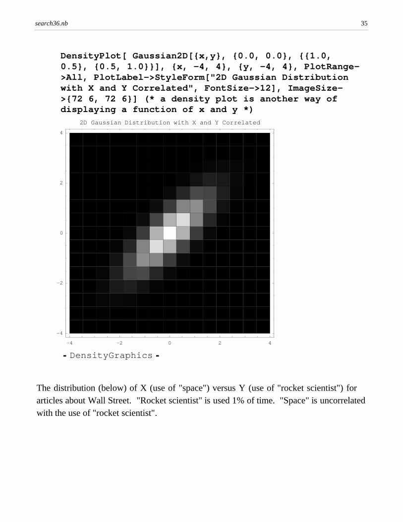
DensityPlot[ Gaussian2D[{x,y}, {0.0, 0.0}, {{1.0, 0.5}, {0.5, 1.0}}], {x, -4, 4}, {y, -4, 4}, PlotRange->All, PlotLabel->StyleForm["2D Gaussian Distribution with X and Y Correlated", FontSize->12], ImageSize->{72 6, 72 6}] (* a density plot is another way of displaying a function of x and y *)

-4 -2 0 2 4

-4

-2

0

2

4


� DensityGraphics �

The distribution (below) of X (use of "space") versus Y (use of "rocket scientist") forarticles about Wall Street. "Rocket scientist" is used 1% of time. "Space" is uncorrelatedwith the use of "rocket scientist".

search36.nb 35

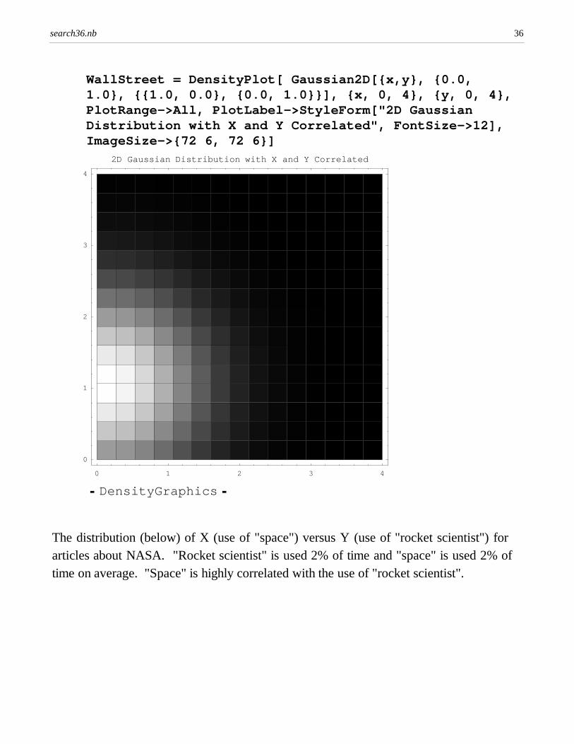
WallStreet = DensityPlot[ Gaussian2D[{x,y}, {0.0, 1.0}, {{1.0, 0.0}, {0.0, 1.0}}], {x, 0, 4}, {y, 0, 4}, PlotRange->All, PlotLabel->StyleForm["2D Gaussian Distribution with X and Y Correlated", FontSize->12], ImageSize->{72 6, 72 6}]

0 1 2 3 4

0

1

2

3

4



The distribution (below) of X (use of "space") versus Y (use of "rocket scientist") forarticles about NASA. "Rocket scientist" is used 2% of time and "space" is used 2% oftime on average. "Space" is highly correlated with the use of "rocket scientist".

search36.nb 36

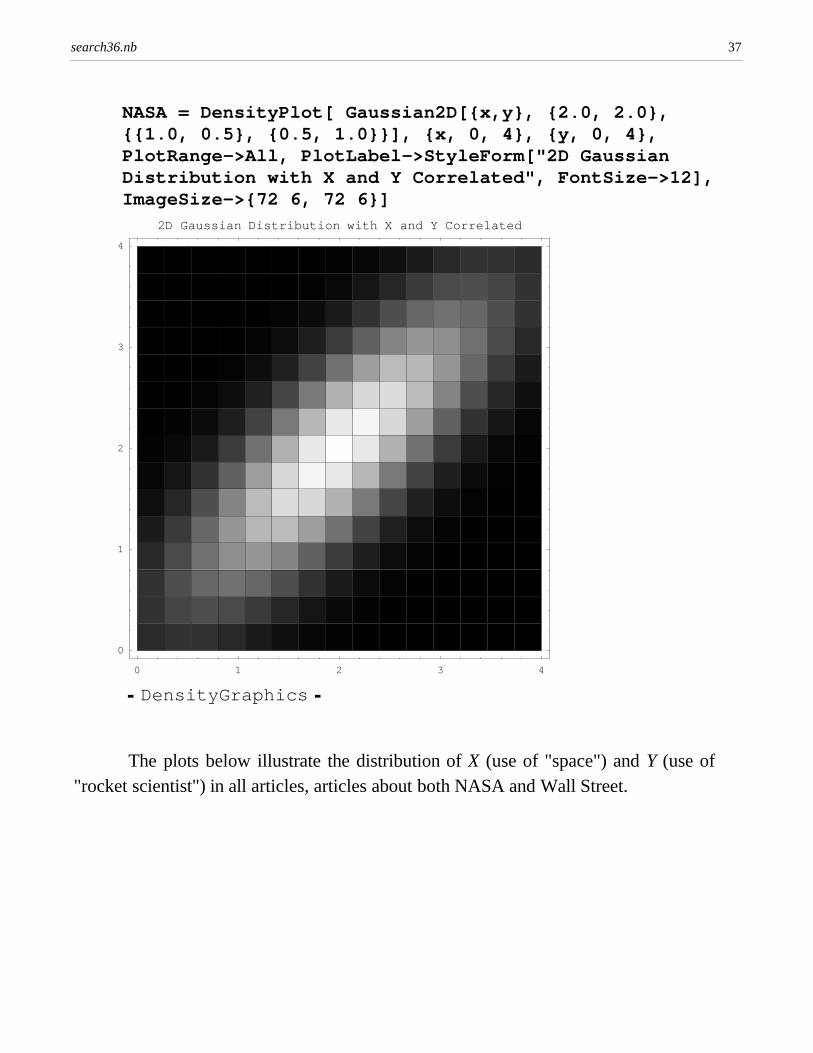
NASA = DensityPlot[ Gaussian2D[{x,y}, {2.0, 2.0}, {{1.0, 0.5}, {0.5, 1.0}}], {x, 0, 4}, {y, 0, 4}, PlotRange->All, PlotLabel->StyleForm["2D Gaussian Distribution with X and Y Correlated", FontSize->12], ImageSize->{72 6, 72 6}]

0 1 2 3 4

0

1

2

3

4



The plots below illustrate the distribution of X (use of "space") and Y (use of"rocket scientist") in all articles, articles about both NASA and Wall Street.

search36.nb 37

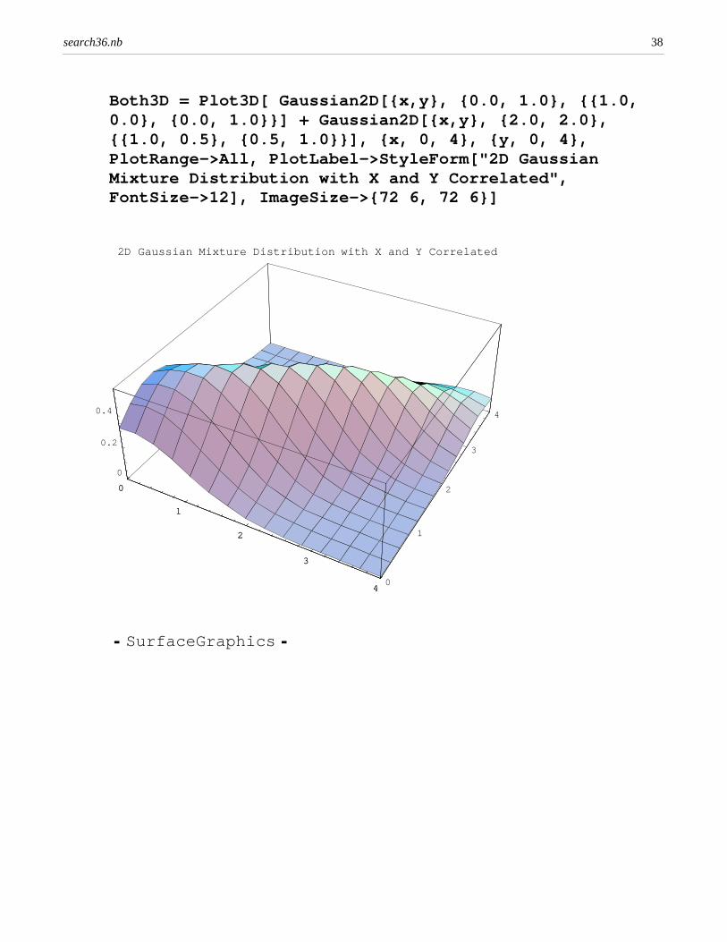
Both3D = Plot3D[ Gaussian2D[{x,y}, {0.0, 1.0}, {{1.0, 0.0}, {0.0, 1.0}}] + Gaussian2D[{x,y}, {2.0, 2.0}, {{1.0, 0.5}, {0.5, 1.0}}], {x, 0, 4}, {y, 0, 4}, PlotRange->All, PlotLabel->StyleForm["2D Gaussian Mixture Distribution with X and Y Correlated", FontSize->12], ImageSize->{72 6, 72 6}]

2D Gaussian Mixture Distribution with X and Y Correlated

0

1

2

3

4 0

1

2

3

4

0

0.2

0.4

0

1

2

3

4


search36.nb 38

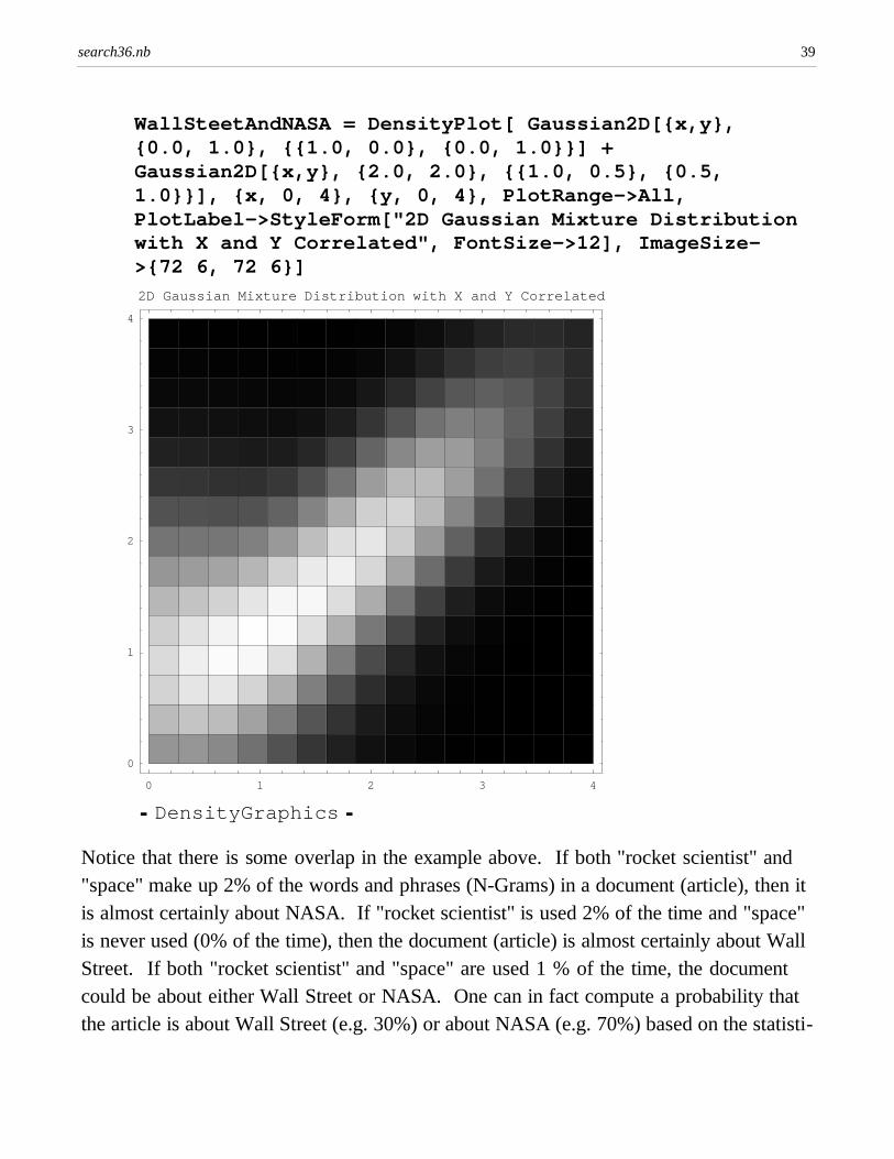
WallSteetAndNASA = DensityPlot[ Gaussian2D[{x,y}, {0.0, 1.0}, {{1.0, 0.0}, {0.0, 1.0}}] + Gaussian2D[{x,y}, {2.0, 2.0}, {{1.0, 0.5}, {0.5, 1.0}}], {x, 0, 4}, {y, 0, 4}, PlotRange->All, PlotLabel->StyleForm["2D Gaussian Mixture Distribution with X and Y Correlated", FontSize->12], ImageSize->{72 6, 72 6}]

0 1 2 3 4

0

1

2

3

4

2D Gaussian Mixture Distribution with X and Y Correlated


Notice that there is some overlap in the example above. If both "rocket scientist" and"space" make up 2% of the words and phrases (N-Grams) in a document (article), then itis almost certainly about NASA. If "rocket scientist" is used 2% of the time and "space"is never used (0% of the time), then the document (article) is almost certainly about WallStreet. If both "rocket scientist" and "space" are used 1 % of the time, the documentcould be about either Wall Street or NASA. One can in fact compute a probability thatthe article is about Wall Street (e.g. 30%) or about NASA (e.g. 70%) based on the statisti

search36.nb 39

cal model of the frequency of "rocket scientist" and "space" in documents. To resolve theoverlaps would require a more sophisticated model of additional N-Grams. For example,one might include the frequency of other words and phrases such as "NASA" or "bondtrader" in the document to improve the accuracy.

Note however that statistical models cannot resolve some cases. They can only imitatehuman understanding. For example, former US Under Secretary of the Treasury andGoldman Sachs executive Neel Kashkari actually worked for NASA prior to moving toWall Street. His NASA background was frequently mentioned in news articles abouthim. Consequently, a statistical model would have difficulty identifying an article aboutNeel Kashkari as an article about Wall Street. Some Wall Street "rocket scientists" actually are rocket scientists. Note also that many articles about NASA discuss the federalbudget, the US Treasury, and other government finance issues making separation basedon fnancial key words and phrases problematic (probably the presence of "GoldmanSachs" in an article would solve the problem in Neel Kashkari's case). Only actual understanding of the text could guarantee a perfect search result in some cases.

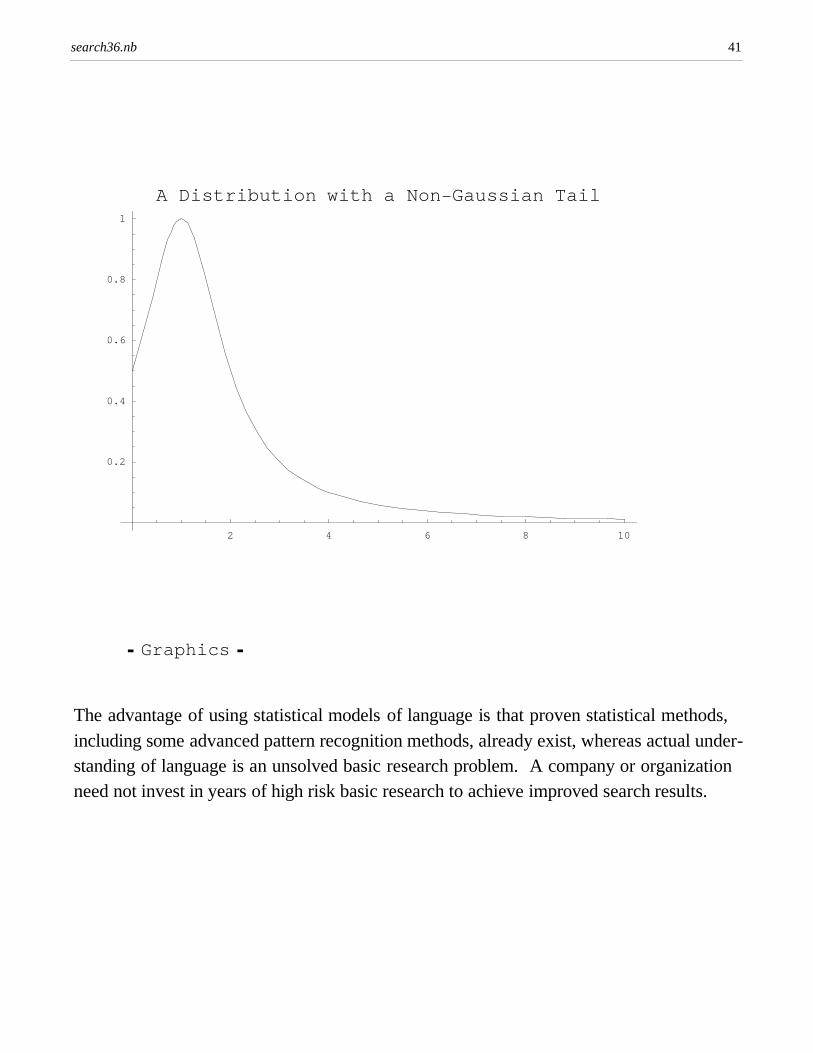
Real world distributions are rarely Gaussians. They are usually more complex and oftenexhibit long "non-Gaussian" tails. The Gaussian is used here only for illustrative purposes. Incidentally, a number of prominent Wall Street financial models including notably the famous Black-Scholes option pricing model and the Gaussian copula model usedto value mortgage backed securities make heavy use of the Gaussian even though mostfinancial assets exhibit non-Gaussian tails. These financial models tend, therefore, tounderstate the risk (and overstate the value) of various financial assets. A real statisticalmodel of English would use more complex models than these simple Gaussian examplesto imitate human understanding of text.

Plot[1.0/(1.0 + (x-1.0)^2), {x, 0.0, 10.0}, PlotLabel->StyleForm["A Distribution with a Non-Gaussian Tail", FontSize->18], ImageSize->{7 72, 7 72}] (* plot the Cauchy-Lorentz function, a simple function with a long tail *)

search36.nb 40

2 4 6 8 10

0.2

0.4

0.6

0.8

1

A Distribution with a Non−Gaussian Tail

� Graphics �

The advantage of using statistical models of language is that proven statistical methods,including some advanced pattern recognition methods, already exist, whereas actual understanding of language is an unsolved basic research problem. A company or organizationneed not invest in years of high risk basic research to achieve improved search results.

search36.nb 41

ü Mathematical Models

The example above is a simple example of type of mathematical model known as a Gaussian Mixture Model (GMM) composed of sums of two or more Gaussian distributions. AGaussian Mixture Model can, with difficulty, approximate any other distribution. Unlessthe distribution being approximated is actually a Gaussian Mixture Model formed from afinite number of Gaussians, the approximation will often require a very large number ofGaussians and still have significant errors. Present day speech recognition algorithms useextremely complex Gaussian Mixture Models to recognize the basic sounds in speech,known as phonemes, for example, the "AH" sound in "father". The Gaussian MixtureModels in speech recognition algorithms today achieve rather limited accuracy, as anyuser of automatic speech recognition systems such as telephone customer service linescan attest to. Other, hopefully simpler, mathematical models may be needed to achievehigher performance in speech recognition or in text search.

Constructing mathematical models that work well is something of a "black art". Thereare standard techniques such as Gaussian Mixture Models but these often require tweaking to use effectively. There are a range of fitting methods used to find mathematicalmodels but these also have many pitfalls and often require "hand tuning" by the mathematical modeler. It usually requires a significant amount of trial and error as well as insight tofind a good mathematical model.

search36.nb 42

à Conclusion

Searching for documents and other items on the Web or computers often takes a longtime. Highly paid professionals spend hours, days, and even longer searching for information on the Web or computers. With professional salaries of tens to hundreds of dollarsper hour, lengthy searches cost hundreds to thousands of dollars per search. Highly paidprofessionals may conduct hundreds, even thousands, of searches each year. The cost oflengthy searches can add up to tens of thousands, hundreds of thousands, even millions ofdollars for just one professional. The cost to organizations with more than one professional can easily be many millions of dollars. The cost to the economy as a whole isprobably billions of dollars. More powerful search engines can save time, money, andfrustration – and ensure success.

Search engines today are based primarily on matching words and phrases often weightedby the popularity of documents, advertising dollars, and other adjustments. In practice,end users often spend many minutes, hours, or days paging through search results and/ortrying many different search words and phrases trying to find a relevant document oritem. More powerful search methods are needed.

The cause of the costly state of search is that present-day search engines do not understand either the search queries or the documents or items searched. More powerfulsearch engines need understanding or a way to emulate aspects of human understandingof text. The dream search engine should find documents or other items by topic, not byword or phrase, and return only documents or items related to the topic of interest.Actual understanding of natural language by computers has proven extremely difficult,like most problems in artificial intelligence (AI), and successes have been few and limited. Hence, search engines continue to rely on simple word and phrase matching.While actual understanding is probably decades, if not centuries, in the future, statisticallanguage processing methods based on the frequency and location of words and phrasesin documents can achieve a degree of searching by topic today.

search36.nb 43

About the Author

John F. McGowan, Ph.D. is a software developer, research scientist, and consultant.He works primarily in the area of complex algorithms that embody advanced mathematical and logical concepts, including speech recognition and video compression technologies. He has extensive experience developing software in C, C++, Visual Basic, Mathematica, and many other programming languages. He is probably best known for hisAVI Overview, an Internet FAQ (Frequently Asked Questions) on the Microsoft AVI(Audio Video Interleave) file format. He has worked as a contractor at NASA AmesResearch Center involved in the research and development of image and video processing algorithms and technology. He has published articles on the origin and evolution oflife, the exploration of Mars (anticipating the discovery of methane on Mars), and cheapaccess to space. He has a Ph.D. in physics from the University of Illinois at Urbana-Champaign and a B.S. in physics from the California Institute of Technology (Caltech).He can be reached at [email protected]

© 2009 John F. McGowan. Ph.D.

search36.nb 44

Documents

Faster, Better, Cheaper Search Engines - John McGowan