Faster, Better: Shear-Wave Velocity to 100 Meters Depth from

347

Bulletin of the Seismological Society of America, 91, 2, pp. 347–364, April 2001

Faster, Better: Shear-Wave Velocity to 100 Meters Depth

from Refraction Microtremor Arrays

by John N. Louie

Abstract Current techniques of estimating shallow shear velocities for assessmentof earthquake site response are too costly for use at most construction sites. Theyrequire large sources to be effective in noisy urban settings or specialized independentrecorders laid out in an extensive array. This work shows that microtremor noiserecordings made on 200-m-long lines of seismic refraction equipment can estimateshear velocity with 20% accuracy, often to 100-m depths. The combination of com-monly available equipment, simple recording with no source, a wavefield transfor-mation data processing technique, and an interactive Rayleigh-wave dispersion mod-eling tool exploits the most effective aspects of the microtremor, spectral analysis ofsurface wave (SASW) and multichannel analysis of surface wave (MASW) techniques.The slowness-frequency wavefield transformation is particularly effective in allowingaccurate picking of Rayleigh-wave phase-velocity dispersion curves despite the pres-ence of waves propagating across the linear array at high apparent velocities, higher-mode Rayleigh waves, body waves, air waves, and incoherent noise. Two locationsillustrate the application of this technique in detail: coincident with a large acceler-ometer microtremor array in Reno, Nevada; and atop a borehole logged for shearvelocity in Newhall, California. Refraction equipment could duplicate microtremorresults above 3 Hz but could not estimate velocities deeper than 100 m. Refractionmicrotremor cannot duplicate the detail in the velocity profile yielded by a suspensionlogger but can match the average velocity of 10- to 20-m depth intervals and suggeststructure below the 100-m logged depth of the hole. Eight additional examples fromsouthern California and New Zealand demonstrate that the refraction microtremortechnique quickly produces good results from a wide range of hard and soft sites.

Motivation

Comprehensive earthquake preparedness requires meth-ods to rapidly assess the possibility of unusually strongshaking at a large number of sites. Estimating shallow shear-velocity structure can be an important component of site-response estimates of possible shaking (Borcherdt andGlassmoyer, 1992; Anderson et al., 1996). The data andanalysis presented in this article show how multichannel ar-rays of lightweight single 8-Hz vertical seismic refractiongeophones can estimate surface-wave velocities to 100-mdepths with very little field effort.

Such seismometers for refraction exploration weigh lessthan 1 kg each. Most universities and engineering consul-tants already possess seismic refraction systems that can dig-itally record between 12 and 48 geophones, or channels,simultaneously. This article shows how to easily deploy suchcommonplace equipment to record background noise, or mi-crotremor, and how the data can yield surface-wave velocitydispersion measurements that constrain shallow shear-velocity structure. The success of these tests suggests that

this technique will efficiently contribute to site-response as-sessments.

The refraction microtremor technique can only resolvevelocity structure to depths of 100 m. Deeper constraintsmay require more conventional seismic survey methods andmicrotremor recordings by broader arrays of more sophis-ticated instruments (Horike, 1985). Satoh et al. (1997) madesuch analyses at the locations of unexpected damage fromthe 1994 Northridge earthquake. Liu et al. (2000) comparedarray results against deep borehole measurements at twoCalifornia sites, finding that array aperture was the limitingfactor in the depth resolution of surface-wave measurements.

A need for the rapid and inexpensive assessment ofearthquake hazard at large numbers of sites has led to thedevelopment of several geophysical testing methods that donot require drilling. The well-known spectral analysis ofsurface waves (SASW) and microtremor array techniquesboth use surface-wave phase information to interpret shear-velocity or rigidity profiles. Other techniques that tried to

employ P waves or S body waves, for example, as presentedin Williams et al. (1994), have not been as successful inmatching ground-shaking or borehole data.

The SASW and MASW Techniques

Nazarian and Stokoe (1984) first described the SASWmethod to the earthquake engineering community. Some-times referred to as CXW (Boore and Brown, 1998), SASWuses an active source of seismic energy, recorded repeatedlyby a pair of 1-Hz seismometers at small (1 m) to large (500m) distances (Nazarian and Desai, 1993). The seismometersare vertical particle-velocity sensors, so shear-velocity pro-files are analyzed on the basis of Rayleigh-wave phase ve-locities interpreted from the recordings. The phase velocitiesare derived purely from a comparison of amplitude and dif-ferential phase spectra computed from each seismometerpair for each source activation, within a fast-Fourier-trans-form oscilloscope (Gucunski and Woods, 1991).

Since the original seismograms are not saved, and allinterpretation is done in the frequency domain, the SASWmethod assumes that the most energetic arrivals recorded areRayleigh waves. Where noise overwhelms the power of theartificial source, as is common in urban areas, or wherebody-wave phases are more energetic than the Rayleighwaves, SASW will not yield reliable results (Brown, 1998;Sutherland and Logan, 1998). The velocities of Rayleighwaves cannot be separated from those of other wave typesin the frequency domain. Boore and Brown (1998) foundthat SASW models consistently underpredicted shallow ve-locities at the sites of six southern California borehole shear-velocity profiles, thus overpredicting ground motions by10% to 50%.

The multichannel analysis of surface waves (MASW)technique (Park et al., 1999) has been developed in responseto the shortcomings of SASW in the presence of noise. Thesimultaneous recording of 12 or more receivers at short (1–2 m) to long (50–100 m) distances from an impulsive orvibratory source gives statistical redundancy to measure-ments of phase velocities. Multichannel data displays in atime-variable frequency format also allow identification andrejection of nonfundamental-mode Rayleigh waves andother coherent noise from the analysis.

Miller et al. (2000) were able to obtain excellent MASWresults in the noisy environment of an operating oil refinery.Using both large and stacked small sources, they were ableto acquire records dominated by fundamental-mode Ray-leigh waves. They also attempted two-dimensional profilingfor lateral anomalies in shear velocity by inverting manyrecords along a profile. Such a profile represents much costlyeffort, similar to that needed for a high-resolution reflectionsurvey, as a large source must be moved along and activatedrepeatedly at a large number of locations.

Simpler Acquisition and More Robust Analysis

The refraction microtremor method combines the urbanutility and ease of microtremor array techniques with the

operational simplicity of the SASW technique and the shal-low accuracy of the MASW technique. By recording urbanmicrotremor on a linear array of a large number of light-weight seismometers, the method achieves fast and easy fielddata collection without any need for the time-consumingheavy source required for SASW and MASW work. By re-taining all the original seismograms and by applying a time-domain velocity analysis technique as is done in MASW, theanalysis described in this article can separate Rayleighwaves from body waves, air waves, and other coherent noise.Transforming the time-domain velocity results into the fre-quency domain allows combination of many arrivals over along time period and yields easy recognition of dispersivesurface waves.

With sponsorship by the U.S. Geological Survey, theSouthern California Earthquake Center, and the U.S. Na-tional Science Foundation; and through collaboration withcolleagues from the Victoria University of Wellington, Shi-mizu Corporation, Kobe University, and the Disaster Pre-vention Research Institute of Kyoto University, this projectcarried out noise surveys at 10 locations in Nevada, southernCalifornia, and New Zealand. Three of these surveys wereblind tests against other techniques. The Reno survey com-bined 1-km-wide arrays of 1-Hz sensors as used by Horike(1985) with 358-m linear arrays of 8-Hz and 4.5-Hz sensorsat the northeast corner of the Reno/Tahoe International Air-port. A 200-m linear noise and refraction array of 8-Hz sen-sors surveyed a ROSRINE borehole at the Newhall Fire Sta-tion in southern California. Also, linear analysis of existing1-Hz array data compared favorably against SASW and seis-mic cone penetrometer profiles in the Parkway neighbor-hood of Wellington, New Zealand.

Method

The refraction microtremor technique is based on twofundamental ideas: (1) common seismic-refraction recordingequipment, set out in a way almost identical to shallow P-wave refraction surveys, can effectively record surfacewaves at frequencies as low as 2 Hz; and (2) a simple, two-dimensional slowness-frequency (p-f ) transform of a micro-tremor record can separate Rayleigh waves from other seis-mic arrivals and allow recognition of true phase velocityagainst apparent velocities.

Use of Seismic Refraction Recording Equipment

Two essential factors that allow exploration equipmentto record surface-wave velocity dispersion, with a minimumof field effort, are (1) the use of a single geophone sensorat each channel, rather than a geophone group array, and(2) the use of a linear spread of 12 or more geophone sensorchannels. Single geophones are the most commonly avail-able type and are typically used for refraction rather thanreflection surveying. The geophones with 8 Hz resonant fre-quency used at most of the ten sites tested here are on the

348 J. N. Louie

Table 1Low-Frequency Coherency Results from 8-Hz Geophones

Preamp Gain 0–5 Hz Filtered 0–25 Hz Filtered Raw

20 dB 32.1 � 10.2% 94.4 � 1.6% 92.2 � 1.6%40 dB 92.9 � 2.2% 96.4 � 3.4% 96.3 � 3.3%60 dB 97.8 � 2.0% 97.2 � 2.4% 96.6 � 2.4%

low end of the frequencies commonly found. They are notunusual among refraction equipment, however.

A geophone group array consists of several sensorswired together to sum electrically, producing a single re-corder input channel. Petroleum-industry seismic-reflectionsurveys use geophone group arrays to cancel surface wavesand other horizontally propagating energy and emphasizevertically propagating reflections. Because of the widespreaduse of group arrays, existing reflection records may not yieldgood results from these surface-wave analysis techniques.New data may have to be taken. If only geophone grouparray strings are available for new recording, they can be setin a cluster, or “potted,” at one effective surface location.Alternatively, the strings might be stretched out perpendic-ularly to the trend of the refraction line, thus mitigating en-ergy propagating across the line while enhancing the re-cording of waves traveling along the line.

A cluster test showed that common, compact seismicrefraction sensors perform very well even if they are set asmuch as 20� off vertical. With no leveling needed, the settingof a 24-channel line of such geophones can take as little asone person-hour. Geophones are usually set below loose sur-face materials and buried under about 10 cm of tamped soilor set into the base of a slice cut into turf and pried openwith a spade. It is easy to pound holes in asphalt pavementwith a short length of 3/8-inch rebar to set the geophonespikes into, if unpaved areas are not available. These smallholes are easily repaired with a quick-setting asphalt patch-ing compound.

Another important component of this experimentalsetup was the use of a relatively long (8–20 m) interval be-tween each geophone along the multichannel spread. Theso-called takeout interval of the cables used for these testsis on the long side of those already in the market, but notunusual. The use of hundreds of meters of multichannel seis-mic recording cable can make deployment of this techniquedifficult in congested urban areas, where the cable wouldhave to be protected at every vehicle crossing. An array ofindependent, stand-alone recorders is easier to deploy overa grid of streets. With careful examination of maps and somescouting, however, at least 200-m lengths of single blockswithout cross streets can be found near almost any desiredsite.

The discussion here is restricted to recordings of singlestraight lines of geophones to evaluate the utility of the sim-plest deployment geometry. As a result, these analyses willcontain energy at apparent phase velocities that are higherthan the true phase velocities. The examples here demon-strate that the lower limit of the apparent phase velocities onthese analyses can be recognized as the true phase velocity.With this ability, it is possible to record with a 200-m re-fraction cable at almost any site, even in very heavily ur-banized areas.

Sensor Accuracy below Their Resonant Frequency. Manyof the experiments reported here used a Bison Galileo-21

48-channel recorder and 8-Hz compact geophones. TheGalileo-21 employs an instantaneous floating-point digitizerto 21-bit floating-point samples. Before digitization, the an-alog signals from the geophones pass through preamplifierswith configurable gain and filter settings. During tests of thesystem’s response to low frequencies, using the 8-Hz geo-phones clustered together, setting the higher ranges of pre-amplifier gain yielded the most coherent recording of noiseand microtremor frequencies below 5 Hz.

Table 1 gives representative correlation coefficients ofcombinations of preamp gain and frequency range for clusternoise records taken on the University of Nevada, Reno cam-pus. The three columns of Table 1 list average correlationcoefficients and their standard deviations between the 24traces of cluster noise records after 0–5 Hz and 0–25 Hzlow-pass filtering, and raw without filtering. These datashow that all instrument preamp gain settings except zerocan accurately record data above 5 Hz; including urbanbackground noise and nearby sledgehammer impacts. Co-herent microtremor at 4 Hz dominates the 0- to 5-Hz filterednoise records. A preamp gain of 40 or above will accuratelyrecord below 5 Hz, although raw or higher-frequency datawill show digitizer clipping from nearby impacts.

A sledgehammer impact closer than 10 m from the ge-ophone will cause physical clipping (pin the seismometer tothe stops). No clipping was observed at lower gain for im-pacts more than 10 m from the cluster. The cluster recordsshow poor but visible coherency below 5 Hz at 20 dB, sug-gesting that any data recorded with similar instrumentsmight yield low-frequency velocities. Table 1 shows cross-correlation tests yielding correlation coefficients of 97.8 �2.0% among geophones in the cluster, at 0–5 Hz with a 60dB gain. Background noise did not saturate digitally at sucha gain, although hammer-blow recordings would.

Other recordings made under similar conditions with aGeometrics R24 seismograph yielding 24-bit integer sam-ples and 12-Hz compact geophones (with the generous co-operation of J. Taber and T. Haver of the Victoria Universityof Wellington, New Zealand) did not need high preamplifiergain to record low-frequency microtremor accurately. Thesetests show that modern refraction geophone transducers,when properly coupled to the ground, can coherently recordfrequencies less than half their resonance frequency. Seis-mographs producing 12- and even 16-bit integer data, on theother hand, probably cannot record low-frequency microtre-mor without an analog high-cut filter.

The very great advantage of the refraction microtremor

Faster, Better: Shear-Wave Velocity to 100 Meters Depth from Refraction Microtremor Arrays 349

technique, from a seismic surveying point of view, is four-fold: it is very fast and inexpensive; it requires only standardrefraction equipment already owned by most consultants anduniversities; it requires no triggered source of wave energy;and it will work best in a seismically noisy urban setting.Traffic and other vehicles, and possibly the wind responsesof trees, buildings, and utility standards provide the surfacewaves this method analyzes.

Velocity Spectral (p-f ) Analysis

The basis of the velocity spectral analysis is the p-stransformation, or slantstack, described by Thorson andClaerbout (1985). This transformation takes a record sectionof multiple seismograms, with seismogram amplitudes rela-tive to distance and time (x-t), and converts it to amplitudesrelative to the ray parameter p (the inverse of apparent ve-locity) and an intercept time s. It is familiar to array analystsas beam forming and has similar objectives to a two-dimensional Fourier-spectrum or f-k analysis as describedby Horike (1985). Clayton and McMechan (1981) and Fuiset al. (1984) used the p-s transformation as an initial step inP-wave refraction velocity analysis.

The p-s transform is a simple line integral across a seis-mic record A(x,t) in distance x and time t

A(p,s) � A(x,t � s � px) dx (1)�x

where the slope of the line p � dt/dx is the inverse of theapparent velocity Va in the x direction. In practice, x is dis-cretized into nx intervals at a finite spacing dx (here usually8–20 m), so x � jdx with an integer j. Likewise time isdiscretized with t � idt (with dt usually 0.001–0.01 sec),giving a discrete form of the p-s transform for negative andpositive p � p0 � ldp and s � kdt called the slantstack:

A(p � p0 � ldp, s � kdt) � (2)nx�1

A(x � jdx, t � idt � s � px)�j�0

starting with a p0 � �pmax. The parameter pmax defines theinverse of the minimum velocity that will be found, usuallyset at 200 m/sec but searched at 100 m/sec or less for par-ticularly soft sites. The parameter np is effectively set to be1 to 2 times nx. Here dp may range from 0.0001 to 0.0005sec/m and is set to cover the interval from �pmax to pmax in2np slowness steps. This will analyze energy propagating inboth directions along the refraction receiver line. Amplitudesat times t � s � px falling between sampled time pointsare estimated by linear interpolation.

The distances used in refraction microtremor analysisare simply distances of geophones from one end of the array.As described by Thorson and Claerbout (1985), the tracesdo not have to sample distance evenly, so the straight arraysanalyzed here are for the convenience of field layout, not for

the convenience of analysis. The intercept times after trans-formation are thus simply arrival times at one end of thearray.

The p-s transformed records contain, in the work here,24 or 48 slowness traces, one or more per offset trace in theoriginal x-t records. Each of these traces contains the linearsum across a record at all intercept times, at a single slow-ness or velocity value. The next step takes each p-s trace inA(p,s) (equation 2) and computes its complex Fourier trans-form FA(p,f ) in the s or intercept time direction:

�i2p fsF (p,f ) � A(p,s)e ds (3)A �s

for which the discrete Fourier transform with f � mdf is

n�1�i2pmdfkdtF (p,f � mdf ) � A(p,s � kdt)e (4)A �

k�0

although, in practice, the fast Fourier transform is mathe-matically equivalent but more efficient. Note that this is aone-dimensional transform that does not affect the slownessor p axis. Achieving good frequency resolution requires re-cording times longer than those typically used in seismicrefraction work. For example, a time sampling dt of 0.001sec requires a record length nt of at least 4000 samples, or4 sec, for df � 0.25 Hz frequency resolution. In this workthe refraction microtremor records range from 20 to 50 secin length.

The power spectrum SA(p,f ) is the magnitude squaredof the complex Fourier transform:

*S (p,f ) � F (p,f ) F (p,f ) (5)A A A

where the * denotes the complex conjugate. This methodsums together two p-s transforms of a record, in both for-ward and reverse directions along the receiver line. To sumenergy from the forward and reverse directions into oneslowness axis that represents the absolute value of p, |p|, theslowness axis is folded and summed about p � 0 with

S (|p|,f ) � [S (p,f )] � [S (�p,f )] (6)A A p�0 A p�0

This completes the transform of a record from distance-time(x-t) into p-frequency (p-f ) space. The ray parameter p forthese records is the horizontal component of slowness (in-verse velocity) along the array. In analyzing more than onerecord from a refraction microtremor deployment, the indi-vidual records’ p-f images SAn

(|p|, f ) are added point-by-point into an image of summed power:

S (|p|,f ) � S (|p|,f ) (7)total � Ann

So the slowness-frequency analysis has produced a recordof the total spectral power in all records from a site, which

350 J. N. Louie

plots within slowness-frequency (p-f ) axes. If one identifiestrends within these axes where a coherent phase has signifi-cant power, then the slowness-frequency picks can be plot-ted on a typical period-velocity diagram for dispersionanalysis.

The p-s transform is linear and invertible and can in factbe completed equivalently in the spatial and temporal fre-quency domains (Thorson and Claerbout, 1985). The trans-form does act as a low-pass 1/frequency filter on the ampli-tudes in the data. However, this filtering does not distort orbias frequencies. The transform stacks along parallel linesto each intercept time, so there is no stretch or frequencydistortion as there is for the normal-moveout or velocitystack along hyperbolae (Thorson and Claerbout, 1985).The transform does produce artifacts, however, smearingdistance-limited or spatially aliased large amplitude wavesover a large range of slownesses. This artifact does not pre-vent the identification of surface-wave dispersion, however.

McMechan and Yedlin (1981) developed the p-f tech-nique and tested it against synthetic surface waves and re-verberations seen on controlled-source multichannel seismicrecords. Park et al. (1998) applied the p-f technique toactive-source MASW records. All phases in the record arepresent in the resulting (p-f ) image that shows the power ateach combination of phase slowness and frequency. Disper-sive phases show the distinct curve of normal modes in low-velocity surface layers: sloping down from high phase ve-locities (low slowness) at low frequencies to lower phasevelocities (high slowness) at higher frequencies. Miller et al.(2000) examine p-f -domain power spectra of MASW recordsalong a profile to define lateral variations in dispersioncurves and thus in shear velocities.

The distinctive slope of dispersive waves is a real ad-vantage of the p-f analysis. Other arrivals that appear inmicrotremor records, such as body waves and air waves,cannot have such a slope. The p-f spectral power image willshow where such waves have significant energy. Even ifmost of the energy in a seismic record is a phase other thanRayleigh waves, the p-f analysis will separate that energy inthe slowness-frequency plot away from the dispersion curvesthis technique interprets. By recording many channels, re-taining complete vertical seismograms, and employing thep-f transform, this method can successfully analyze Ray-leigh dispersion where SASW techniques cannot.

Rayleigh Phase-Velocity Dispersion Picking

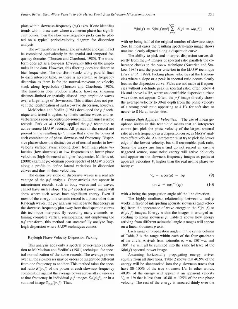
This analysis adds only a spectral power-ratio calcula-tion to McMechan and Yedlin’s (1981) technique, for spec-tral normalization of the noise records. The average powerover all the slownesses may be orders of magnitude differentfrom one frequency to another. This method takes the spec-tral ratio R(|p|,f ) of the power at each slowness-frequencycombination against the average power across all slownessesat that frequency in individual p-f images SA(|p|,f ), or in asummed image Stotal(|p|,f ). Thus,

np�1

R(|p|, f ) � S(|p|, f )np/[ S(|p| � ldp, f )] (8)�l�0

with np being half of the original number of slowness steps2np. In most cases the resulting spectral-ratio image showsmaxima clearly aligned along a dispersion curve.

The ability to pick and interpret dispersion curves di-rectly from the p-f images of spectral ratio parallels the co-herence checks in the SASW technique (Nazarian and Sto-koe, 1984) and the power criterion in the MASW technique(Park et al., 1999). Picking phase velocities at the frequen-cies where a slope or a peak in spectral ratio occurs clearlylocates the dispersion curve. Picks are not made at frequen-cies without a definite peak in spectral ratio, often below 4Hz and above 14 Hz, where an identifiable dispersive surfacewave does not appear. Often, the p-f image directly showsthe average velocity to 30-m depth from the phase velocityof a strong peak ratio appearing at 4 Hz for soft sites ornearer to 8 Hz at harder sites.

Avoiding High Apparent Velocities. The use of linear ge-ophone arrays in this technique means that an interpretercannot just pick the phase velocity of the largest spectralratio at each frequency as a dispersion curve, as MASW anal-yses effectively do. An interpreter must try to pick the loweredge of the lowest-velocity, but still reasonable, peak ratio.Since the arrays are linear and do not record an on-linetriggered source, some noise energy will arrive obliquelyand appear on the slowness-frequency images as peaks atapparent velocities Va higher than the real in-line phase ve-locity v:

V � v/cos(a) � 1/p (9)a

�1or: a � cos (vp) (10)

with a being the propagation angle off the line direction.The highly nonlinear relationship between a and p

works in favor of interpreting accurate slowness (and veloc-ity) from the appearance of wave energy in the S(|p|, f ) orR(|p|, f ) images. Energy within the images is arranged ac-cording to linear slowness p. Table 2 shows how energyarriving from different azimuthal angle a ranges will appearon a linear slowness p axis.

Each range of propagation angle a in the center columnof Table 2 is the range within each of the four quadrantsof the circle. Arrivals from azimuths a, �a, 180��a, and180� �a will all be summed into the same |p| trace of theS(|p|, f ) spectral-power image.

Assuming horizontally propagating energy arrivesequally from all directions, Table 2 shows that 40.9% of theenergy will be slantstacked into the p slowness traces thathave 80–100% of the true slowness 1/v. In other words,40.9% of the energy will appear at an apparent velocityVa � 1/p that is less than 1/0.80 � 125% of the true phasevelocity. The rest of the energy is smeared thinly over the


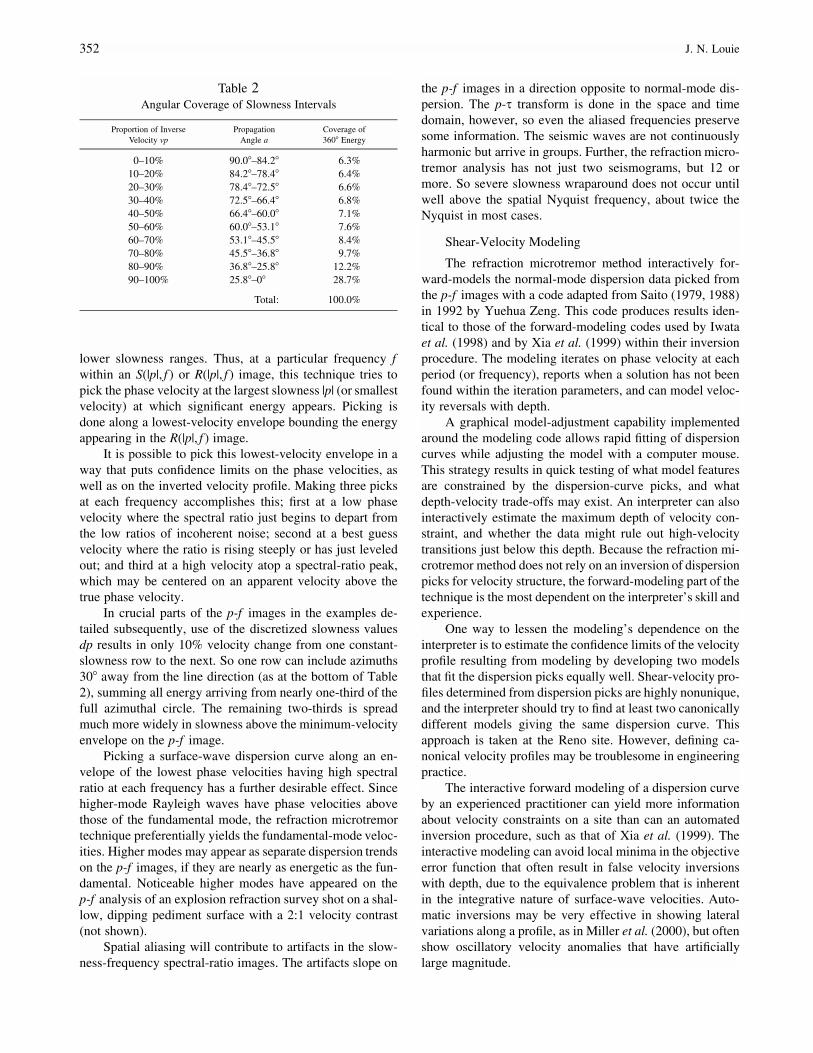
Table 2Angular Coverage of Slowness Intervals

Proportion of InverseVelocity vp

PropagationAngle a

Coverage of360� Energy

0–10% 90.0�–84.2� 6.3%10–20% 84.2�–78.4� 6.4%20–30% 78.4�–72.5� 6.6%30–40% 72.5�–66.4� 6.8%40–50% 66.4�–60.0� 7.1%50–60% 60.0�–53.1� 7.6%60–70% 53.1�–45.5� 8.4%70–80% 45.5�–36.8� 9.7%80–90% 36.8�–25.8� 12.2%90–100% 25.8�–0� 28.7%

Total: 100.0%

lower slowness ranges. Thus, at a particular frequency fwithin an S(|p|, f ) or R(|p|, f ) image, this technique tries topick the phase velocity at the largest slowness |p| (or smallestvelocity) at which significant energy appears. Picking isdone along a lowest-velocity envelope bounding the energyappearing in the R(|p|, f ) image.

It is possible to pick this lowest-velocity envelope in away that puts confidence limits on the phase velocities, aswell as on the inverted velocity profile. Making three picksat each frequency accomplishes this; first at a low phasevelocity where the spectral ratio just begins to depart fromthe low ratios of incoherent noise; second at a best guessvelocity where the ratio is rising steeply or has just leveledout; and third at a high velocity atop a spectral-ratio peak,which may be centered on an apparent velocity above thetrue phase velocity.

In crucial parts of the p-f images in the examples de-tailed subsequently, use of the discretized slowness valuesdp results in only 10% velocity change from one constant-slowness row to the next. So one row can include azimuths30� away from the line direction (as at the bottom of Table2), summing all energy arriving from nearly one-third of thefull azimuthal circle. The remaining two-thirds is spreadmuch more widely in slowness above the minimum-velocityenvelope on the p-f image.

Picking a surface-wave dispersion curve along an en-velope of the lowest phase velocities having high spectralratio at each frequency has a further desirable effect. Sincehigher-mode Rayleigh waves have phase velocities abovethose of the fundamental mode, the refraction microtremortechnique preferentially yields the fundamental-mode veloc-ities. Higher modes may appear as separate dispersion trendson the p-f images, if they are nearly as energetic as the fun-damental. Noticeable higher modes have appeared on thep-f analysis of an explosion refraction survey shot on a shal-low, dipping pediment surface with a 2:1 velocity contrast(not shown).

Spatial aliasing will contribute to artifacts in the slow-ness-frequency spectral-ratio images. The artifacts slope on

the p-f images in a direction opposite to normal-mode dis-persion. The p-s transform is done in the space and timedomain, however, so even the aliased frequencies preservesome information. The seismic waves are not continuouslyharmonic but arrive in groups. Further, the refraction micro-tremor analysis has not just two seismograms, but 12 ormore. So severe slowness wraparound does not occur untilwell above the spatial Nyquist frequency, about twice theNyquist in most cases.

Shear-Velocity Modeling

The refraction microtremor method interactively for-ward-models the normal-mode dispersion data picked fromthe p-f images with a code adapted from Saito (1979, 1988)in 1992 by Yuehua Zeng. This code produces results iden-tical to those of the forward-modeling codes used by Iwataet al. (1998) and by Xia et al. (1999) within their inversionprocedure. The modeling iterates on phase velocity at eachperiod (or frequency), reports when a solution has not beenfound within the iteration parameters, and can model veloc-ity reversals with depth.

A graphical model-adjustment capability implementedaround the modeling code allows rapid fitting of dispersioncurves while adjusting the model with a computer mouse.This strategy results in quick testing of what model featuresare constrained by the dispersion-curve picks, and whatdepth-velocity trade-offs may exist. An interpreter can alsointeractively estimate the maximum depth of velocity con-straint, and whether the data might rule out high-velocitytransitions just below this depth. Because the refraction mi-crotremor method does not rely on an inversion of dispersionpicks for velocity structure, the forward-modeling part of thetechnique is the most dependent on the interpreter’s skill andexperience.

One way to lessen the modeling’s dependence on theinterpreter is to estimate the confidence limits of the velocityprofile resulting from modeling by developing two modelsthat fit the dispersion picks equally well. Shear-velocity pro-files determined from dispersion picks are highly nonunique,and the interpreter should try to find at least two canonicallydifferent models giving the same dispersion curve. Thisapproach is taken at the Reno site. However, defining ca-nonical velocity profiles may be troublesome in engineeringpractice.

The interactive forward modeling of a dispersion curveby an experienced practitioner can yield more informationabout velocity constraints on a site than can an automatedinversion procedure, such as that of Xia et al. (1999). Theinteractive modeling can avoid local minima in the objectiveerror function that often result in false velocity inversionswith depth, due to the equivalence problem that is inherentin the integrative nature of surface-wave velocities. Auto-matic inversions may be very effective in showing lateralvariations along a profile, as in Miller et al. (2000), but oftenshow oscillatory velocity anomalies that have artificiallylarge magnitude.

352 J. N. Louie

In geophysical exploration work using other integrativefields such as gravity, magnetics, and resistivity, problemswith automated inversions exaggerating anomalies have ledto the widespread current practice of interactive forwardmodeling. Microtremor analysis done by Liu et al. (2000)completely avoids modeling of picked dispersions by simplycomparing array dispersion data against dispersions forwardmodeled from borehole data. The interactive forward mod-eling of dispersion curves, though, is no slower than inver-sion procedures and allows the fitting of a simple model inless than a minute using popular computer platforms. Themain difficulty with interactive modeling is to reduce theprocess of testing hypotheses and estimating confidence lim-its to a set of practical procedures that will not require ex-tensive retraining by practitioners.

A simple method, more independent of the observerthan developing a set of canonical models, is to fit modelsto the high- and low-velocity confidence limits of the dis-persion picks. This procedure will produce extremal velocityprofiles at the limits of the velocity range allowed by thedispersion data, a technique discussed for the Reno andNewhall examples below. With 95–99% of the minimum-velocity energy in the p-f images usually falling between thepicked velocity extremes, there is similar confidence in thevelocity ranges produced.

If higher-mode Rayleigh dispersion picks have beenmade, those can be modeled as well with the codes employedhere. Another possible problem is the lack of information onP-wave velocities or densities in modeling Rayleigh disper-sion curves. All of the modeling done for this article hasassumed a Poisson ratio of 0.25, which is often far from thetruth in shallow soils. Experimentation with the interactivemodeling tool suggests that even huge changes in Poissonratio or density will only change modeled shear velocitiesby less than 10% in the process of fitting Rayleigh-wavevelocity spectra. Lay and Wallace (1995, p. 122) show thatthe Rayleigh phase velocity in a half space will change onlyfrom 89% to 95% of the shear velocity, as the Poisson ratioranges from 0.1 to 0.4.

These factors suggest that Rayleigh dispersion curvesare good indicators of shear-velocity structure and poor in-dicators of shallow P-velocity structure. A Jacobian analysisof Rayleigh dispersion inversion by Xia et al. (1999) sup-ports this suggestion. Liu et al. (2000) also maintain thatRayleigh phase-velocity measurements can only constrainshear velocity. Since the refraction microtremor method usesessentially phase information from multichannel seismic re-cordings to estimate surface-wave phase velocities, deter-mination of near-surface shear velocities is an attainablegoal.

Results

Described here in detail are two tests of the refractionmicrotremor technique, done at locations where the mostdefinitive corroborating data exist. The first test was against

a more traditional accelerometer microtremor array (as inHorike, 1985; or Liu et al., 2000) in Reno, Nevada. Thesecond test was against the shear-velocity suspension log ofa 100-m-deep borehole in Newhall, California. Described inless detail subsequently is the application of this techniqueat eight other locations in Wellington, New Zealand, and insouthern California. This p-f analysis technique has alsobeen applied extensively to explosion refraction records.

In all trials the method has produced reasonable shear-velocity results to 50–150 m depth, in good agreement withall available data. However, the two cases discussed first arethose for which the best shear-velocity data from indepen-dent measurements were available. They were effectivelyblind prediction tests, as was the work of Liu et al. (2000),since the independent data were not examined before refrac-tion microtremor results were developed. True blind predic-tion has not been attempted, however; it would requiredrilling and logging of a borehole only after refractionmicrotremor results had been published.

Tests Against a Microtremor AccelerometerArray in Reno, Nevada

On 22 July 1997 and 18 October 2000, University ofNevada, Reno, staff and students performed linear refractionarray recording tests on the property of the Reno/Tahoe In-ternational Airport, at the southwest corner of Rock Blvd.and Mill Street in Reno, Nevada (Fig. 1). The site is next tothe north end of the airport’s main runways and about 1 kmnorth of a site at which the UNR Seismological Lab maderecordings of aftershocks of the 12 September 1994 DoubleSpring Flat event (Ni et al., 1997). The site is bladed soiland gravel fill, covered by organic materials and silt depos-ited by a major Truckee River flood in January 1997. Thesite is about 300 m south of the river.

In the 1997 test two arrays of 24 8-Hz geophones spacedat 15.24 m were spread out in approximately W–E andN–S directions from the intersection. Each geophone wasplanted in a hole 10 cm deep, covered with soil, and tampedlightly. The several 48-sec noise records recorded by theBison Galileo-21 had a 4 msec sampling interval and a 60dB preamplifier gain. Fieldwork for that test required morethan 8 person-hours because of the use of 48 channels overa 720 m total array length.

The 2000 test placed one N–S array of 15 RefTek RT-125 Texan recorders, with 24-bit fixed-point digitizers and4.5-Hz geophones (Figure 1). The geophones were spacedat 20 m for an overall array length of 280 m. Geophoneplants were similar, and five 50-sec noise records were taken.Fieldwork for that test required only 4 person-hours.

Wave Sources. One of the records triggered in 1997 wasat the time of an approximately 3000 kg ripple-fired exca-vation blast 16 km to the south. Synchronizing watches overa cell phone link with an observer at the blast site providedtiming to �2 seconds. The N–S channel 1–18 section of the


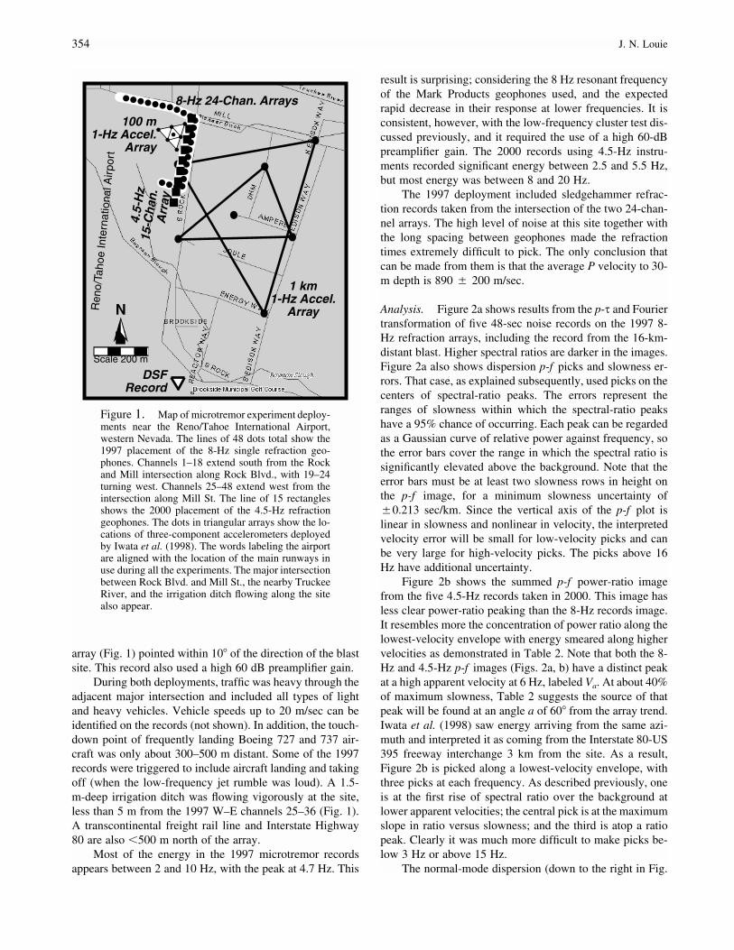
Figure 1. Map of microtremor experiment deploy-ments near the Reno/Tahoe International Airport,western Nevada. The lines of 48 dots total show the1997 placement of the 8-Hz single refraction geo-phones. Channels 1–18 extend south from the Rockand Mill intersection along Rock Blvd., with 19–24turning west. Channels 25–48 extend west from theintersection along Mill St. The line of 15 rectanglesshows the 2000 placement of the 4.5-Hz refractiongeophones. The dots in triangular arrays show the lo-cations of three-component accelerometers deployedby Iwata et al. (1998). The words labeling the airportare aligned with the location of the main runways inuse during all the experiments. The major intersectionbetween Rock Blvd. and Mill St., the nearby TruckeeRiver, and the irrigation ditch flowing along the sitealso appear.

array (Fig. 1) pointed within 10� of the direction of the blastsite. This record also used a high 60 dB preamplifier gain.

During both deployments, traffic was heavy through theadjacent major intersection and included all types of lightand heavy vehicles. Vehicle speeds up to 20 m/sec can beidentified on the records (not shown). In addition, the touch-down point of frequently landing Boeing 727 and 737 air-craft was only about 300–500 m distant. Some of the 1997records were triggered to include aircraft landing and takingoff (when the low-frequency jet rumble was loud). A 1.5-m-deep irrigation ditch was flowing vigorously at the site,less than 5 m from the 1997 W–E channels 25–36 (Fig. 1).A transcontinental freight rail line and Interstate Highway80 are also �500 m north of the array.

Most of the energy in the 1997 microtremor recordsappears between 2 and 10 Hz, with the peak at 4.7 Hz. This

result is surprising; considering the 8 Hz resonant frequencyof the Mark Products geophones used, and the expectedrapid decrease in their response at lower frequencies. It isconsistent, however, with the low-frequency cluster test dis-cussed previously, and it required the use of a high 60-dBpreamplifier gain. The 2000 records using 4.5-Hz instru-ments recorded significant energy between 2.5 and 5.5 Hz,but most energy was between 8 and 20 Hz.

The 1997 deployment included sledgehammer refrac-tion records taken from the intersection of the two 24-chan-nel arrays. The high level of noise at this site together withthe long spacing between geophones made the refractiontimes extremely difficult to pick. The only conclusion thatcan be made from them is that the average P velocity to 30-m depth is 890 � 200 m/sec.

Analysis. Figure 2a shows results from the p-s and Fouriertransformation of five 48-sec noise records on the 1997 8-Hz refraction arrays, including the record from the 16-km-distant blast. Higher spectral ratios are darker in the images.Figure 2a also shows dispersion p-f picks and slowness er-rors. That case, as explained subsequently, used picks on thecenters of spectral-ratio peaks. The errors represent theranges of slowness within which the spectral-ratio peakshave a 95% chance of occurring. Each peak can be regardedas a Gaussian curve of relative power against frequency, sothe error bars cover the range in which the spectral ratio issignificantly elevated above the background. Note that theerror bars must be at least two slowness rows in height onthe p-f image, for a minimum slowness uncertainty of�0.213 sec/km. Since the vertical axis of the p-f plot islinear in slowness and nonlinear in velocity, the interpretedvelocity error will be small for low-velocity picks and canbe very large for high-velocity picks. The picks above 16Hz have additional uncertainty.

Figure 2b shows the summed p-f power-ratio imagefrom the five 4.5-Hz records taken in 2000. This image hasless clear power-ratio peaking than the 8-Hz records image.It resembles more the concentration of power ratio along thelowest-velocity envelope with energy smeared along highervelocities as demonstrated in Table 2. Note that both the 8-Hz and 4.5-Hz p-f images (Figs. 2a, b) have a distinct peakat a high apparent velocity at 6 Hz, labeled Va. At about 40%of maximum slowness, Table 2 suggests the source of thatpeak will be found at an angle a of 60� from the array trend.Iwata et al. (1998) saw energy arriving from the same azi-muth and interpreted it as coming from the Interstate 80-US395 freeway interchange 3 km from the site. As a result,Figure 2b is picked along a lowest-velocity envelope, withthree picks at each frequency. As described previously, oneis at the first rise of spectral ratio over the background atlower apparent velocities; the central pick is at the maximumslope in ratio versus slowness; and the third is atop a ratiopeak. Clearly it was much more difficult to make picks be-low 3 Hz or above 15 Hz.

The normal-mode dispersion (down to the right in Fig.

354 J. N. Louie

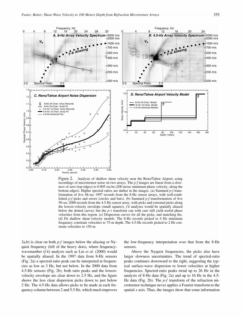
Figure 2. Analysis of shallow shear velocity near the Reno/Tahoe Airport, usingrecordings of microtremor noise on two arrays. The p-f images are linear from a slow-ness of zero (top edges) to 0.005 sec/m (200 m/sec minimum phase velocity, along thebottom edges). Higher spectral ratios are darker in the images. (a) Summed p-f trans-formation of five 48-sec 1997 records from the 8-Hz sensor arrays, with well-estab-lished p-f picks and errors (circles and bars). (b) Summed p-f transformation of five50-sec 2000 records from the 4.5-Hz sensor array, with picks and extremal picks alongthe lowest-velocity envelope (small squares). f-k analyses would be spatially aliasedbelow the dotted curves; but the p-s transform can with care still yield useful phasevelocities from this region. (e) Dispersion curves for all the picks, and matching fits.(d) Fit shallow shear-velocity models. The 8-Hz records picked to 4 Hz minimumfrequency constrain velocities to 75-m depth. The 4.5-Hz records picked to 2 Hz con-strain velocities to 150 m.

2a,b) is clear on both p-f images below the aliasing or Ny-quist frequency (left of the heavy dots), where frequency-wavenumber (f-k) analysis such as Liu et al. (2000) wouldbe spatially aliased. In the 1997 data from 8-Hz sensors(Fig. 2a) a spectral-ratio peak can be interpreted at frequen-cies as low as 3 Hz, but not below. In the 2000 data from4.5-Hz sensors (Fig. 2b), both ratio peaks and the lowest-velocity envelope are clear down to 2.5 Hz, and the figureshows the less clear dispersion picks down to just below2 Hz. The 4.5-Hz data allows picks to be made at each fre-quency column between 2 and 5.5 Hz, which much improves

the low-frequency interpretation over that from the 8-Hzsensors.

Above the Nyquist frequencies, the picks also havelarger slowness uncertainties. The trend of spectral-ratiopeaks continues downward to the right, suggesting the typ-ical surface-wave dispersion to lower velocities at higherfrequencies. Spectral-ratio peaks trend up to 26 Hz in theanalysis of 8-Hz data (Fig. 2a) and up to 16 Hz in the 4.5-Hz data (Fig. 2b). The p-f transform of the refraction mi-crotremor technique never applies a Fourier transform to thespatial x axis. Thus, the images show that some information


can be recovered at high frequencies where f-k analyseswould fail.

The strongest peaks of spectral ratio are at 12 Hz inFigure 2a and 10 Hz in Figure 2b. These peaks arise fromwaves that are spatially truncated by the edges of the arrays.The truncation leaves the smeared and frequency-shifted ar-tifacts that arch up and to the right in both images, essentiallyartifacts of the p-s transform (equations 1 and 2). Frequencywraparound smears the high-spectral ratio points in bothplots subparallel to the dotted Nyquist curves. Clearly, how-ever, these artifacts slope down to the left on the p-f plotsand do not interfere with picking normal-mode dispersiontrends.

In the areas of the p-f plots that would be aliased in anf-k analysis, the slantstack is still sensitive to the energy con-centration of the group arrival across 12 or more traces inthe record. This factor keeps the velocity range of the ali-ased, smeared peaks limited. The frequency wraparound andsmearing show the frequency shift error of the peaks. Theseshifts do not extend beyond the limited shifts of the stronggroup arrival on Figure 2a at 12 Hz or on Figure 2b at10 Hz. In this way, picks from the aliased areas of the ve-locity spectral plots could have 4–8 Hz of frequency error,up to 25%.

Examination of the 1997 raw blast record after 0–5 Hzlow-pass filtering (not shown) identified surface wave arri-vals with a 0.43 � 0.03 km/sec group velocity and 0.86 to1.3 km/sec phase velocity. These arrivals are not clearly sep-arable in Figure 2a, although they contribute to a smear ofmoderately high spectral ratios at 6 Hz and below.

Apparent Phase Velocities. Figure 2a includes the spectralsum of four noise records and the 16-km distant blast record.The minimum apparent velocity, or true phase velocity, ofthe dispersed surface wave sums well. The sum includedboth the E–W and N–S parts of the arrays, showing the re-sulting coherence and preponderance of waves traveling nearthe true velocities. On both p-f images, Va labels a significantspectral-ratio peak that does not contribute to the minimum-velocity interpretation. But the Va peaks do not interfere withmaking the correct interpretation.

If one assumes an even distribution of energy arrivingfrom all directions, over all these 48-sec records, then Table2 makes clear the reason for the coherent summation at thetrue velocity. The nonlinearity of the cosine that divides thereal velocity to produce the apparent velocity allows a thirdof the energy from many random directions to contribute tothe observed peak, no more than 20% higher than the truevelocity. The remaining two-thirds is spread much morewidely in slowness and is visible in Figures 2a and b as abackground of slightly higher spectral ratios, at velocitiesabove the true dispersion curve. With the summing of spec-tra from records of two perpendicular linear arrays in Figure2a, the nonlinear concentration of energy toward the truevelocities on the p-f image is even more pronounced.

The superimposed line on Figure 2a traces the disper-

sion trend from 0.50 km/sec at 4 Hz down to 0.25 km/secat 26 Hz. The slowness accuracy of this trend appears to beabout the slowness sample interval of the p-s transform(0.213 sec/km in that image). Thus, at the low-velocity end,the phase-velocity estimates should be accurate to within�0.015 km/sec. Frequency accuracy within this plot is notas good as the frequency sampling but can be �0.25 Hz orbetter, in picking spectral-ratio peaks outside the aliasedarea.

Velocity Modeling. Figure 2c graphs the picked disper-sions, error bars, and extremal picks from both p-f images.It also shows the fits within the errors and extremes of syn-thetic dispersion curves from the models in Figure 2d. Ex-tensive interactive testing with the forward-modeling appli-cation shows that picks constrain the 0–9 m depth shearvelocity very well at 0.28 km/sec, the 9–40 m depth at 0.52km/sec, as well as the 9 and 40 m depths of the velocityincreases. The 0.68 km/sec velocity below 40 m can tradeoff against the depth and velocity of the deeper interface at77–156 m (Fig. 2d). The aliasing and resulting frequencyshifts of the picks above 12 Hz do not have a significanteffect on the modeling.

The picks from the 8-Hz-sensor data, at 4-Hz minimumfrequency, cannot constrain velocity below a 75-m depth.The interpreter, in the absence of other data, placed a 1.55km/sec layer at 77-m depth. The picks from the 4.5-Hz-sensor data extend down to 2 Hz, allowing the interpreter toplace a higher-velocity 1.98 km/sec interface deeper, at 156m. Thus using lower-frequency sensors probably doubledthe maximum depth of velocity constraint, to about 150 m(question marks on figure 2d). In both cases, the higherphase velocities picked at the lower frequencies demand avelocity increase at some depth below the depth of con-straint. Being in essence depth-averaged velocities, thehigher phase velocities constrain the ratio of the depth andvelocity, but not either one individually.

In modeling the dispersion-curve picks of Figure 2c, theinterpreter attempted to develop canonically different mod-els that fit the data equally well. The differences in the twomodels presented in Figure 2d is in the number of shallowlayers and in the depth and velocity of the deepest layer. Thethree-layer model presents an extreme hypothesis for thedeepest layer, showing it at the minimum possible depth andminimum possible velocity. Both the test models, plus themodels fitting the extremal picks, fit to nearly the same ve-locity at 9–77 m depths and also give a narrow velocity rangefor the shallowest 0- to 9-m layer. The three- and four-layermodels have almost identical average velocities for the 0- to30-m-depth range, of 456 and 448 m/sec, respectively.

Comparison with Accelerometer Results. In December1997 colleagues from Shimizu Corp. and Kyoto and KobeUniversities tested at the Reno/Tahoe Airport site a nested-triangle array of seven 1-Hz, three-component accelerome-ters. This is the type of accelerometer array they have de-

356 J. N. Louie

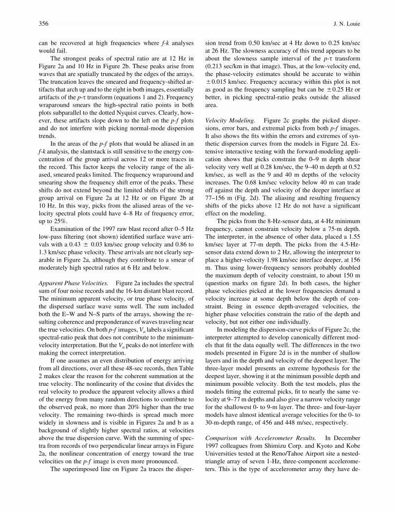
Figure 3. Comparison of phase-velocityspectra near the Reno/Tahoe Airport from threemicrotremor noise recording techniques. Tri-angles with error bars were picked from f-kanalysis of broadband accelerometer array re-cords by Iwata et al. (1998), yielding the modelplotted with a thin solid line. Open circlesand the thick dashed lines show the lower-frequency part of microtremor analysis using8-Hz refraction equipment and the p-s andFourier transformation method, from Figure 2.Squares and a thick solid line show the resultsof the same analysis on the coincident array of4.5-Hz refraction recorders. The thin dashedline is a model computed from a 30 m boreholelog by Ni et al. (1997).

ployed for microtremor noise recording in Japan andCalifornia (for example: Satoh et al., 1997), and is almostidentical to the techniques of Liu et al. (2000). They re-corded both 100-m and 1-km-aperture arrays at the Reno/Tahoe Airport site (Fig. 1).

Each seismometer recorded independently, with timingprovided by GPS clocks, so distributing the array over anarea of several blocks was not difficult. Setting out eachreceiver, however, required a painstaking leveling process,as the 1-Hz accelerometers are far more sensitive to levelingerrors than are the velocity sensors of the refraction equip-ment. The fieldwork for each array required more than 10person-hours and used custom equipment costing more than$100,000.

Iwata et al. (1998) showed the results of their analysisfor the airport site. They analyzed only vertical-componentnoise records. Total recorded time was about one hour; cer-tain slices of their data several minutes long yielded goodresults in their moving-window f-k domain analysis (verymuch like the analysis presented by Liu et al. (2000). Thefrequency range of their phase velocity estimates (Fig. 3)overlaps that of the refraction experiments (from Fig. 2) be-tween 2 and 7 Hz. At 3 Hz they determined a 0.475 � 0.05km/sec velocity, and at 7 Hz it was 0.45 � 0.02 km/sec.From Figure 2a, the 8-Hz-sensor refraction microtremor pickat 4 Hz agrees with their results at 0.47 km/sec (Fig. 3). FromFigure 2b, the 4.5-Hz-sensor refraction microtremor pick ishigher at 0.51 km/sec, with extremes at 0.46 and 0.60 km/sec. At 8 Hz, the refraction microtremor picks are at 0.42 �0.02 km/sec. The lack of lower-frequency data preventscomparison against their results below 2 Hz. The data ofinterest for the prediction of shallow site amplification, from4 Hz and up, are virtually identical.

Because of the close spacing and large number of chan-nels allowed by the 8-Hz refraction equipment, it producessurface-wave dispersion most easily interpreted betweenabout 7 and 16 Hz, as Figure 2a shows. The modeling inFigures 2c and 2d suggested that this range puts good con-straints on shear velocities within 75 m of the surface. Dis-persion is often interpretable in the p-f results at higher fre-

quencies where an f-k analysis is impossible due to spatialaliasing. The refraction equipment could more accurately as-sess shear velocity at very shallow 1- to 10-m depths, whilethe 2D array of 1-Hz instruments was needed to estimate thevelocity profile from 100-m to 1-km depths.

The amplification analysis of Ni et al. (1997), based ona nearby 30-m-deep acoustic log and weak-motion records,suggests similar shallow velocities, with modeled dispersioncurves matching those of Iwata et al. (1998) above 3 Hz.Gravity work across the Reno basin by Abbott and Louie(2000a) shows a depth to andesite basement at the RenoAirport site of 400 m. Nearby water wells penetrating 200–300 m make it unlikely that the 77–156 m interface couldbe basement. It is more likely the base of Quaternary allu-vium and the top of a Miocene-Pliocene diatomaceous sand-stone that underlies the entire basin (Abbott and Louie,2000a). Shallow models from noise recorded on refractionequipment could not derive basin sediment thickness here,although the lower-frequency accelerometer data of Iwata etal. (1998) could do so.

Test at the ROSRINE Borehole in Newhall, California

On 13 September 1996 the Resolution of Site ResponseIssues from the Northridge Earthquake (ROSRINE) project(http://geoinfo.usc.edu/rosrine; Nigbor et al., 1997) col-lected an OYO suspension P- and S-wave velocity log at theLos Angeles County Fire Station in Newhall, California. InFebruary 2000, with sponsorship from the Southern Cali-fornia Earthquake Center, and assistance from Los AngelesCounty Fire Dept. personnel and the County Flood ControlDistrict, University of Nevada, Reno staff located the site ofthe ROSRINE borehole and performed refraction and micro-tremor experiments.

The refraction microtremor experiment employed a200-m-long array of 24 8-Hz refraction geophones along theasphalt-paved access road at the side of a 4-m-deep concrete-lined flood channel. The 200-m array was centered 4 m fromthe ROSRINE hole. Noise records 30 and 60 sec long and areversed sledgehammer refraction profile were recorded. A10-sec section of the first noise record taken appears in Fig-


ure 4a. Using the same equipment as with the 8-Hz Reno/Tahoe Airport deployment, the microtremor fieldwork inNewhall required less than 6 person-hours, with a field crewof three. Time at the site was extended, however, by rainshowers, recording of a large number of noise records, andby the hammer refraction recording.

Noise Sources. This part of Newhall is densely suburban,with heavily trafficked streets only 100–200 m apart, andfully built up. San Fernando Road, a six-lane artery, is only75 m from the array. Frequent commuter trains were running100 m away. The raw microtremor record in Figure 4a showsidentifiable Rayleigh groups with 100–200 m/sec velocities,at a relatively high frequency of 18 Hz. The surface wavemarked on Figure 4a, one example of the many present,probably originated close to the array. The lower-frequencymicrotremor is not easily seen in the figure, which includesfrequencies up to 20 Hz.

Analysis. For the Newhall example, just the analysis of thefirst 30-sec noise record taken is shown here. If the refractionmicrotremor techniques can be sufficiently accurate on justone record, then prolonged field recording efforts are notneeded. The p-f analysis of this 30-sec noise record is Figure4b. From 3–12 Hz, the p-f image shows a clear energy cutoffat a minimum-velocity envelope. The energy of obliquely-propagating waves is broadly distributed across high appar-ent velocities above this envelope. Arrivals at many differentapparent velocities form a broad ramp in spectral ratio, butthe cutoff of high spectral-ratio values against the true phase-velocity envelope is clear from 3 to 12 Hz (as shown byTable 2). At frequencies below 3 Hz, and in the area of f-kaliasing, this envelope is not as clear. There are a few spec-tral-ratio peaks in these areas still aligned with the dispersionenvelope.

The dispersion picks follow the lowest-velocity enve-lope at the base of the high spectral ratios in the image (Fig.4b). The area of pick confidence is between the lowest ve-locity where spectral ratios rise above those of uncorrelatednoise (white in Fig. 4b) and the higher velocity at the top ofthe ratio peak (black in Fig. 4b). The best pick was madewithin this range where the ratio slope is steepest, as for theReno 4.5-Hz data in Figure 2b. The three phase-velocityvalues at one frequency constitute the dispersion pick (filledsquares in Fig. 4c) and its uncertainty within extremal values(open squares in Fig. 4c). Dispersion picking is possiblewhere an F-K analysis would spatially alias (right of thethick dashed line in Fig. 4b), although the p-f artifacts pro-duce larger p uncertainties there.

Velocity Modeling. Figure 4c shows just the dispersioncurve with increasing velocity uncertainty at larger periods,interactively modeled with the velocity profile of Figure 4d(bold line). The modeled profile is an excellent match to theROSRINE logged shear velocity (thick gray line). The 8-m-thick shallowest layer with 210 m/sec shear velocity com-pares well with the log, which starts at a 2-m depth and

varies from 178–238 m/sec to 8-m depth. The 370 m/secmodeled layer from 8 to 34-m depth averages across a stronggradient in the log from 219 to 685 m/sec over the samedepth range. Below 34 m, the shear-velocity log has about10% variability with a standard deviation of 77 m/sec butmaintains the 105.2-m maximum logged depth, a 741 m/secaverage. The 34 to 125-m-depth model layer has a velocityof 620 m/sec, which is just 16% low.

The bias of the interactive modeling process towardfewer layers, 7- to 100-m thick, is clear in this comparison.Since the phase-velocity dispersion data effectively integratevelocities over substantial depth ranges, modeling resultscould never match the detail of the shear-velocity log. In thelog, velocities can change by 30% over a few meters. Thislack of detail in the modeled velocity profile is no impedi-ment to site-response evaluation, however. The amplifica-tion of earthquake waves by site conditions is also an inte-grative process. As long as the velocity results are accuratein terms of averages over 5 to 100-m depth ranges, accurateprediction of linear site amplification effects is assured(Borcherdt and Glassmoyer, 1992; Boore and Brown, 1998;Brown, 1998).

The uncertain longest-period picks of the dispersioncurve (Fig. 4c) suggest a velocity increase at an interfacebelow the 100-m maximum logged depth (question mark inFig. 4d). However, the low-frequency dispersion picks can-not control the trade-off between the depth and velocity ofthis interface. Experimentation shows that many modelscould match the dispersions in Figure 4c. Both the depth andthe velocity of the deepest layer are highly nonunique andvery poorly determined at this site by the dispersions downonly to 2 Hz. In this case, at least the ROSRINE log showsthat the interface is deeper than 100 m. This fact suggeststhe refraction microtremor method could estimate velocityaccurately to 100 m at this site.

The Newhall example demonstrates a simpler methodof finding velocity constraints than that used for the Renosite. Developing a set of canonical models, essentially in-dependent geological hypotheses, is too time-consuming forpractical use. Modeling a single dispersion curve with theinteractive tool is still a task that relies on some training,and tutorial exercises have been written to teach undergrad-uates how to perform the modeling effectively.

A top-down approach is most effective, matching phasevelocities with layer velocity adjustments, starting at the sur-face layer (e.g., fitting the picks on Fig. 4c below 0.1-secperiod first). Cusps and increases in slope of the dispersioncurve (as at 0.12 sec, 0.25 sec, and 0.45 sec in Fig. 4c) arematched by adjusting layer thicknesses. Following such aprocedure, it is possible to model velocities in about oneminute, since only a small number of layers is used.

Here the extremal velocity limits are found by fittingnot only the best picks (filled boxes on Fig. 4c) but also,separately, the highest-velocity picks, and the lowest-veloc-ity picks of the confidence limits (open squares on Fig. 4c).This procedure results in three models, one central and two

358 J. N. Louie

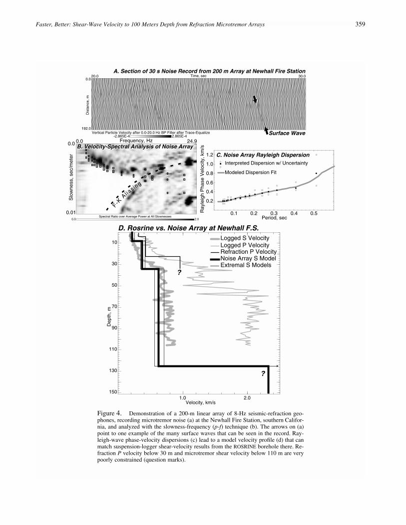
Figure 4. Demonstration of a 200-m linear array of 8-Hz seismic-refraction geo-phones, recording microtremor noise (a) at the Newhall Fire Station, southern Califor-nia, and analyzed with the slowness-frequency (p-f) technique (b). The arrows on (a)point to one example of the many surface waves that can be seen in the record. Ray-leigh-wave phase-velocity dispersions (c) lead to a model velocity profile (d) that canmatch suspension-logger shear-velocity results from the ROSRINE borehole there. Re-fraction P velocity below 30 m and microtremor shear velocity below 110 m are verypoorly constrained (question marks).


that represent the upper and lower-velocity extremes of con-fidence in the pick of the central model. The thin lines onFigure 4d show the velocity profiles that result from thisprocedure. For the poorly constrained deepest layer (ques-tion mark in Fig. 4d), the minimum extremal model had thesame velocity as the central model, while the maximum ex-tremal model had a velocity of 3.5 km/sec, off the plot. Forthese data adjustment of layer thicknesses was not necessaryin the process of creating the extremal models.

P-Wave Refraction Results. The refraction experimentsconducted at Newhall show a shallow P-wave velocity of328–408 m/sec. At 23-m depth, the P-wave velocity in-creases to 970 m/sec (thin black line in Fig. 4d). These val-ues also agree well with the OYO suspension P-velocity log(thin gray line in Fig. 4d). Naturally a simple refraction in-terpretation cannot yield the detail of the suspension log. Butthe velocities and refractor depth agree well with the steepvelocity gradient in the log from 26- to 34-m depth.

Both the 23-m deep P-wave refractor and the 34-m deepincrease in shear velocity may represent the same interface,possibly a transition to more consolidated or clay-rich Qua-ternary alluvium. The interface is seen as both P- and S-wave velocity gradients over the 23- to 34-m depth range inthe logs. The 11-m mismatch in depth between the refractionand shear-velocity modeling could be eliminated by biasingthe refraction interpretation within its confidence limits orby inserting another layer into the shear-velocity model.First arrivals from 50 stacked hammer blows could only beseen to 130-m distances in this noisy area. As a result, therefraction data were not sensitive to either the logged P-velocity increase at 60-m depth or the bottom of Quaternarysediments at 125 m (or deeper) interpreted from the Rayleighdispersion.

Stability of Data and Analysis. The record analyzed inFigure 4 is only the first of 14 noise records taken at theNewhall site. The experiment recorded 10 records 30 seclong, 5 with 2-msec sampling and 5 with 1-msec sampling.Four additional records were 60 sec long, with 1-msec timesampling. Summed p-f images were computed of the five 2-msec-sampled 30-sec records, of the five 1-msec sampled30-sec records, and of the four 60-sec records. The p-f im-ages are very similar to the single-record image, except forthe increased concentration of energy close to the true phasevelocity as was seen in the Reno summed-record analysis.

Each summed p-f image was picked independently. Thepicks all agree well with the single-record picks of Figure4c, with two exceptions. The summed-record picks showphase velocities 15% to 30% higher than the single-recordpicks between periods of 0.3 and 0.42 sec. This is the periodrange most sensitive to the velocity of the 34- to 125-m-deeplayer, which was 16% slower in the single-record analysisthan in the shear-velocity log. Modeling the picks from thissummed-record p-f image gave the layer a 707 m/sec veloc-ity, only 5% lower than the 741 m/sec average in the log.

The other exception arose in trying to alter how one ofthe summed-record p-f images was picked. The five 30-secrecords with 1-msec sampling produced a p-f image thatseemed more distinctly peaked along the true-velocity dis-persion curve than the other images. Accordingly, it waspicked not along the low-velocity envelope but atop the cen-ter of its spectral-ratio peaks (not shown). At periods be-tween 0.22 and 0.38 sec, this procedure yielded phase ve-locities that were up to two times larger than the velocitiespicked from all other Newhall p-f images. Fitting the bestpicks at the ratio peaks yielded a velocity for the 34- to 125-m-deep layer of 993 m/sec, 34% higher than the 741 m/secaverage of the shear-velocity log for that depth range. For arandomly oriented single, straight-line noise array, pickingthe lowest-velocity envelope appears to be the most accurateprocedure.

Extremal models matching the dispersion-envelopepick confidence limits show high confidence that modelinghas estimated velocities to 100-m depth with 15% accuracyat Newhall, comparable to the total variability of the loggedshear velocity over 5-m depth ranges. Rayleigh phase-velocity dispersion modeling matches the logged shear ve-locity despite a significant increase in the Poisson’s ratio at50-m depth. With the match to logged velocities shown inFigure 4, the cheap and rapid linear-array microtremor tech-nique promises almost the depth and velocity resolution ofthe SASW and MASW techniques, but at lower cost since noartificial energy source is needed.

Additional Tests

Wellington, New Zealand. Ground-shaking hazard assess-ments have been underway for some years in New Zealand’sWellington metropolitan area (e.g., Van Dissen et al., 1992).Geotechnical surveys of shear-velocity profiles have onlytaken place in two suburbs underlain by particularly softsediments, known as Parkway and Porirua. In the Parkwaysuburb, Duggan (1997) conducted gravity and triggered-source seismic-refraction and reflection surveys, but notnoise recordings. These techniques revealed 75 m of low-velocity lacustrine sediments overlying Mesozoic grey-wacke basement. Yu and Taber (1998) recorded noise andlocal events on a temporary network of 24 1-Hz stationsabout 0.5 km across. Barker (1996) made seismic cone-penetrometer profiles at three sites in Parkway. Sutherlandand Logan (1998) provide shear velocities to 20-m depthfrom SASW surveys at a site in Parkway.

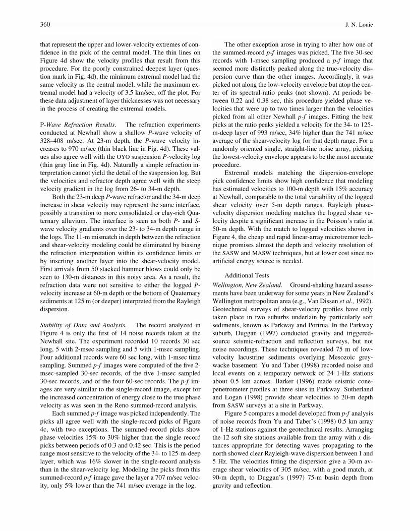
Figure 5 compares a model developed from p-f analysisof noise records from Yu and Taber’s (1998) 0.5 km arrayof 1-Hz stations against the geotechnical results. Arrangingthe 12 soft-site stations available from the array with x dis-tances appropriate for detecting waves propagating to thenorth showed clear Rayleigh-wave dispersion between 1 and5 Hz. The velocities fitting the dispersion give a 30-m av-erage shear velocities of 305 m/sec, with a good match, at90-m depth, to Duggan’s (1997) 75-m basin depth fromgravity and reflection.

360 J. N. Louie

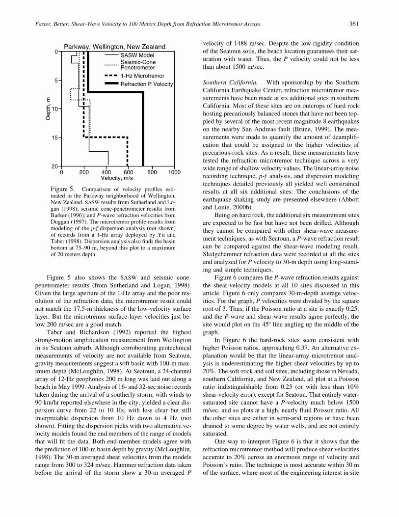
Figure 5. Comparison of velocity profiles esti-mated in the Parkway neighborhood of Wellington,New Zealand. SASW results from Sutherland and Lo-gan (1998); seismic cone-penetrometer results fromBarker (1996); and P-wave refraction velocities fromDuggan (1997). The microtremor profile results frommodeling of the p-f dispersion analysis (not shown)of records from a 1-Hz array deployed by Yu andTaber (1998). Dispersion analysis also finds the basinbottom at 75–90 m, beyond this plot to a maximumof 20 meters depth.

Figure 5 also shows the SASW and seismic cone-penetrometer results (from Sutherland and Logan, 1998).Given the large aperture of the 1-Hz array and the poor res-olution of the refraction data, the microtremor result couldnot match the 17.5-m thickness of the low-velocity surfacelayer. But the microtremor surface-layer velocities just be-low 200 m/sec are a good match.

Taber and Richardson (1992) reported the higheststrong-motion amplification measurement from Wellingtonin its Seatoun suburb. Although corroborating geotechnicalmeasurements of velocity are not available from Seatoun,gravity measurements suggest a soft basin with 100-m max-imum depth (McLoughlin, 1998). At Seatoun, a 24-channelarray of 12-Hz geophones 200 m long was laid out along abeach in May 1999. Analysis of 16- and 32-sec noise recordstaken during the arrival of a southerly storm, with winds to90 km/hr reported elsewhere in the city, yielded a clear dis-persion curve from 22 to 10 Hz, with less clear but stillinterpretable dispersion from 10 Hz down to 4 Hz (notshown). Fitting the dispersion picks with two alternative ve-locity models found the end members of the range of modelsthat will fit the data. Both end-member models agree withthe prediction of 100-m basin depth by gravity (McLoughlin,1998). The 30-m averaged shear velocities from the modelsrange from 300 to 324 m/sec. Hammer refraction data takenbefore the arrival of the storm show a 30-m averaged P

velocity of 1488 m/sec. Despite the low-rigidity conditionof the Seatoun soils, the beach location guarantees their sat-uration with water. Thus, the P velocity could not be lessthan about 1500 m/sec.

Southern California. With sponsorship by the SouthernCalifornia Earthquake Center, refraction microtremor mea-surements have been made at six additional sites in southernCalifornia. Most of these sites are on outcrops of hard rockhosting precariously balanced stones that have not been top-pled by several of the most recent magnitude 8 earthquakeson the nearby San Andreas fault (Brune, 1999). The mea-surements were made to quantify the amount of deamplifi-cation that could be assigned to the higher velocities ofprecarious-rock sites. As a result, these measurements havetested the refraction microtremor technique across a verywide range of shallow velocity values. The linear-array noiserecording technique, p-f analysis, and dispersion modelingtechniques detailed previously all yielded well constrainedresults at all six additional sites. The conclusions of theearthquake-shaking study are presented elsewhere (Abbottand Louie, 2000b).

Being on hard rock, the additional six measurement sitesare expected to be fast but have not been drilled. Althoughthey cannot be compared with other shear-wave measure-ment techniques, as with Seatoun, a P-wave refraction resultcan be compared against the shear-wave modeling result.Sledgehammer refraction data were recorded at all the sitesand analyzed for P velocity to 30-m depth using long-stand-ing and simple techniques.

Figure 6 compares the P-wave refraction results againstthe shear-velocity models at all 10 sites discussed in thisarticle. Figure 6 only compares 30-m-depth average veloc-ities. For the graph, P velocities were divided by the squareroot of 3. Thus, if the Poisson ratio at a site is exactly 0.25,and the P-wave and shear-wave results agree perfectly, thesite would plot on the 45� line angling up the middle of thegraph.

In Figure 6 the hard-rock sites seem consistent withhigher Poisson ratios, approaching 0.37. An alternative ex-planation would be that the linear-array microtremor anal-ysis is underestimating the higher shear velocities by up to20%. The soft-rock and soil sites, including those in Nevada,southern California, and New Zealand, all plot at a Poissonratio indistinguishable from 0.25 (or with less than 10%shear-velocity error), except for Seatoun. That entirely water-saturated site cannot have a P-velocity much below 1500m/sec, and so plots at a high, nearly fluid Poisson ratio. Allthe other sites are either in semi-arid regions or have beendrained to some degree by water wells, and are not entirelysaturated.

One way to interpret Figure 6 is that it shows that therefraction microtremor method will produce shear velocitiesaccurate to 20% across an enormous range of velocity andPoisson’s ratio. The technique is most accurate within 30 mof the surface, where most of the engineering interest in site


Figure 6. Comparison of 30-m averaged velocityestimates at ten sites. Shear velocities derived frommicrotremor modeling are plotted on the horizontalaxis. Shear velocities estimated from coincidentP-wave refraction results are plotted on the vertical,after assuming a Poisson ratio of 0.25 in convertingto a shear velocity. In the Santa Clarita Valley andwestern Mojave Desert of southern California: NFS,Newhall Fire Station (Fig. 4); MCS, Mill Creek Sum-mit; GLR, Gleason Road 0.5 km from MCS; ANB An-telope Buttes; LJB, Lovejoy Buttes; ALC, Aliso Can-yon; and PIB, Piute Butte. In Nevada; RNO, Reno/Tahoe Airport (Fig. 1 and 2). In Wellington, NewZealand: PKY, Parkway (Fig. 5); STN, Seatoun.

conditions lies. Refraction microtremor will go beyond a 30-m depth, however, to produce useful constraints on shearvelocity to a 100-m depth at most sites.

Conclusions

The 10 sites described in this article are all those testedwith refraction microtremor to date, for which a corroborat-ing velocity estimate is available from any other technique.Quiet rural sites (such as Piute Butte) do not yield refractionmicrotremor results as easily interpreted as results fromnoisy urban sites. Despite this variation in quality, every dataset collected with this technique has yielded interpretablevelocities. No site has been culled from the analysis here,and every data set collected has been analyzed.

The refraction microtremor method does not explicitlycorrect the apparent velocities of waves traveling obliquelyto the array. Instead it relies on the stacking of waves trav-eling in all directions, the greater precision of the array forvelocities along its length, and a procedure for picking thedispersion curve along a lowest-velocity envelope in the p-f images. This technique matched the shallower part of theresults from microtremor recording in Reno of the type orig-

inated by Horike (1985) and yielded better shear-velocityestimates within 30 m of the surface. Comparison of theseresults against the shear-velocity log of the ROSRINE bore-hole at the Newhall County Fire Station proved the tech-nique to be accurate, matching the log to within 15%. Eightadditional tests in southern California and New Zealandshow the refraction microtremor technique can quickly findthe 30-m-average shear velocity to better than 20% accuracy.

These tests show that common seismic refraction equip-ment can yield accurate surface-wave dispersion informationfrom microtremor noise. Configurations of 12 to 48 singlevertical, 8–12 Hz exploration geophones can give surface-wave phase velocities at frequencies as low as 2 Hz and ashigh as 26 Hz. This range is appropriate for constrainingshear velocity profiles from the surface to 100-m depths. Theheavy triggered sources of seismic waves used by the SASWand MASW techniques to overcome noise are not needed,saving considerable survey effort. This microtremor tech-nique may be most fruitful, in fact, where noise is mostsevere. Proof of this technique suggests that rapid and veryinexpensive shear-velocity evaluations are now possible atthe most heavily urbanized sites and at sites within busytransportation corridors.

In addition, limited resources for earthquake-hazardevaluation can now be stretched to measure at 3 to 10 timesas many sites as was possible in the past. A possible appli-cation of this method would be to gather large numbers of100-m shear-velocity profiles across mapped soil types usedto predict regional shaking hazards (as by Borcherdt andGlassmoyer, 1992). Hazard classification schemes and haz-ard maps based on soil mapping could be verified againstthe velocity profiles. In addition, the multiple velocity mea-surements for each soil type would contribute a velocity var-iance to soil-type-based probabilistic seismic hazard map-ping efforts.

Another application of this technique is that it is nowpossible to estimate shear velocities at one site for 10%–30% of the cost of SASW, MASW, borehole, or cone-penetrometer evaluations. In regions where the earthquakehazard or risk is not high enough to justify the cost of ex-isting methods for site evaluation, this technique will allowa quick and affordable site study. The refraction microtremortechnique requires as few as two person-hours, including allanalysis, and equipment with a capital cost now as low as$10,000 (for a 12-channel refraction system). Even homebuilders might now be able to afford a shear-velocity eval-uation at every home site. If engineers and builders find thistechnique useful, seismologists can look forward to an ex-plosion in the number of available shallow site characteri-zations.

Acknowledgments

This research was supported in part by the U.S. Geological SurveyNational Earthquake Hazards Reduction Program under Contract NumberN117292, with coinvestigators J. G. Anderson, F. Su, and Y. Zeng; as well

362 J. N. Louie

as by the Southern California Earthquake Center, with coinvestigatorsR. Anooshehpoor and J. Brune. SCEC is funded by NSF Cooperative Agree-ment EAR-8920B6 and USGS Cooperative Agreements 14-08-0001-A0899and 1434-HQ-97AG01718. The SCEC contribution number for this articleis 515. The W. M. Keck Foundation generously donated the seismic re-fraction equipment to the Mackay School of Mines, University of Nevada,Reno. Reftek 4.5-Hz Texan recorders and software were loaned by the IRIS/PASSCAL instrument center at New Mexico Tech, with training providedby S. Azevedo. T. Iwata, H. Kawase, T. Satoh, Y. Kakehi, and K. Irikuraof the Disaster Prevention Research Institute, Kyoto University, Kobe Uni-versity, and Shimizu Corporation graciously made the accelerometer de-ployments, performed data analyses, and also helped support the author’ssabbatical research. Further crucial sabbatical assistance and collaborationwere generously provided by E. Smith, M. Savage, J. Taber, T. Haver, M.Robertson, and R. Neal of the Victoria University of Wellington, NewZealand. Refraction instruments were deployed in Reno and southern Cali-fornia with valuable assistance from K. Smith, R. Anooshehpoor, R. E.Abbott, G. Ichinose, M. Herrick, M. Engle, A. Pancha, J. Skalbeck, and C.Mann. Caithness Power Corp. and Mike Tyler of Cal-Neva Drilling andBlasting kindly provided timing information on their 3000-kg constructionblast. The Reno/Tahoe International Airport Authority generously providedaccess to the Reno site. The Los Angeles County Flood Control Districtand the Los Angeles County Fire Station in Newhall were very helpful inproviding access to the ROSRINE site in Newhall, California.

References

Abbott, R. E., and J. N. Louie (2000a). Depth to bedrock using gravimetryin the Reno and Carson City, Nevada area basins, Geophysics 65,340–350.

Abbott, R. E., and J. N. Louie (2000b). High shear wave velocities underprecarious rock sites might be enough to explain their existence nearthe San Andreas fault (abstract), EOS Trans. AGU 81, no. 48, F821.

Anderson, J. G., Y. Lee, Y. Zeng, and S. Day (1996). Control of strongmotion by the upper 30 meters, Bull. Seism. Soc. Am. 86, 1749–1759.

Boore, D. M., and L. T. Brown (1998). Comparing shear-wave velocityprofiles from inversion of surface-wave phase velocities with down-hole measurements: systematic differences between the CXW methodand downhole measurements at six USC strong-motion sites, Seism.Res. Lett. 69, 222–229.

Borcherdt, R. D., and G. Glassmoyer (1992). On the characteristics of localgeology and their influence on ground motions generated by the LomaPrieta earthquake in the San Francisco Bay region, California, Bull.Seism. Soc. Am. 82, 603–641.

Brown, L. T. (1998). Comparison of Vs profiles from SASW and boreholemeasurements at strong motion sites in southern California, Master’sThesis, University of Texas, Austin, 349 pp.

Brune, J. N. (1999). Precariously balanced rocks along the Mojave sectionof the San Andreas fault, California: constraints on ground motionfrom great earthquakes, Seism. Res. Lett. 70, 29–33.

Clayton, R. W., and G. A. McMechan (1981). Inversion of refraction databy wavefield continuation, Geophysics 46, 860–868.

Duggan, E. B. (1997). Shallow seismic structure of Parkway basin, Wain-uiomata, New Zealand, Bachelor’s Thesis, School of Earth Sciences,Victoria University of Wellington, Wellington, New Zealand, 116 pp.

Fuis, G., W. Mooney, J. Healy, G. McMechan, and W. Lutter (1984). Aseismic refraction survey of the Imperial Valley region, California, J.Geophys. Res. 89, 1165–1190.

Gucunski, N., and R. D. Woods (1991). Instrumentation for SASW testingin Recent Advances in Instrumentation, Data Acquisition, and Testingin Soil Dynamics, Geotechnical Special Publ. No. 29: American So-ciety of Civil Engineers, New York, p. 1–16.

Horike, M. (1985). Inversion of phase velocity of long-period microtremorsto the S-wave-velocity structure down to the basement in urbanizedareas, J. Phys. Earth. 33, 59–96.

Iwata, T., H. Kawase, T. Satoh, Y. Kakehi, K. Irikura, J. N. Louie, R. E.

Abbott, and J. G. Anderson (1998). Array microtremor measurementsat Reno, Nevada, USA (abstract), EOS Trans. AGU 79, no. 45,p. F578.

Lay, T., and T. C. Wallace (1995). Modern Global Seismology, AcademicPress, San Diego, 521 pp.

Liu, H. P., D. M. Boore, W. B. Joyner, D. H. Oppenheimer, R. E. Warrick,W. Zhang, J. C. Hamilton, and L. T. Brown (2000). Comparison ofphase velocities from array measurements of Rayleigh waves asso-ciated with microtremor and results calculated from borehole shear-wave velocity profiles, Bull. Seism. Soc. Am. 90, 666–678.

McLoughlin, C. (1998). The Seatoun basin, Wellington, a geophysical in-vestigation: evidence from gravity and electrical resistivity data,Bachelor’s Thesis, School of Earth Sciences, Victoria University ofWellington, Wellington, New Zealand, 65 pp.

McMechan, G. A., and M. J. Yedlin (1981). Analysis of dispersive wavesby wave field transformation, Geophysics 46, 869–874.

Miller, R. D., C. B. Park, J. M. Ivanov, J. Xia, D. R. Laflen, and C. Gratton(2000). MASW to investigate anomalous near-surface materials at theIndian Refinery in Lawrenceville, Illinois, Kansas Geol. Surv. Open-File Rept. 2000-4, Lawrence, Kansas, 48 pp. (Electronic version athttp://www.kgs.ukans.edu/Geophysics/Reports2/Illinois.pdf )

Nazarian, S., and M. R. Desai (1993). Automated surface wave method:field testing, J. Geotech. Eng. 119, 1094–1111.

Nazarian, S., and K. H. Stokoe II (1984). In situ shear wave velocities fromspectral analysis of surface waves in Proceedings of the World Con-ference on Earthquake Engineering, Vol. 8, San Francisco, 21–28July.

Ni, S.-D., R. Siddharthan, and J. G. Anderson (1997). Characteristics ofnonlinear response of deep saturated soil deposits, Bull. Seism. Soc.Am. 87, 342–355.

Nigbor, R., C. Roblee, R. Pyke, J. Schneider, W. Silva, R. A. Steller, andM. Vucetic (1997). Resolution of site response issues from the North-ridge earthquake (ROSRINE) (abstract), Seism. Res. Lett. 68, p. 303.

Park, C. B., R. D. Miller, and J. Xia (1998). Imaging dispersion curves ofsurface waves on multichannel record in 68th Annual InternationalSoc. Explor. Geophys., New Orleans, Sept. 13–18, Expanded Ab-stracts, p. 1377–1380.

Park, C. B., R. D. Miller, and J. Xia (1999). Multi-channel analysis ofsurface waves, Geophysics 64, 800–808.

Saito, M. (1979). Computations of reflectivity and surface wave dispersioncurves for layered media. I. Sound wave and SH wave, Butsuri-Tanko32, no. 5, 15–26.

Saito, M. (1988). Compound matrix method for the calculation of spheroi-dal oscillation of the Earth, Seism. Res. Lett. 59, 29.

Satoh, T., H. Kawase, T. Iwata, and K. Irikura (1997). S-wave velocitystructures in the damaged areas during the 1994 Northridge earth-quake based on array measurements of microtremors (abstract), EOSTrans. AGU 78, no. 46, 432.

Sutherland, A. J., and T. C. Logan (1998). SASW measurement for thecalculation of site amplification, Earthquake Commission ResearchProject 97/276, Central Laboratories Report 98-522422, Lower Hutt,New Zealand, 22 pp.

Taber, J. J., and W. P. Richardson (1992). Frequency dependent amplifi-cation of weak ground motions in Wellington City and the Kapiticoast, Client report to Wellington Regional Council, New Zealand,53 pp.

Thorson, J. R., and J. F. Claerbout (1985). Velocity-stack and slant-stackstochastic inversion, Geophysics 50, 2727–2741.

Van Dissen, R. J., J. J. Taber, W. R. Stephenson, S. Sritharan, S. A. L.Read, G. H. McVerry, G. D. Dellow, and P. R. Barker (1992). Earth-quake ground shaking hazard assessment for the Lower Hutt and Po-rirua areas, Bull. New Zealand Natl. Soc. Earthquake Eng. 25, 286–302.

Williams, R. A., E. Cranswick, K. W. King, D. L. Carver, and D. M. Worley(1994). Site-response models from high-resolution seismic reflectionand refraction data recorded in Santa Cruz, California, in The LomaPrieta, California, Earthquake of October 17, 1989: Strong Ground


Motion R. D. Borcherdt (Editor), U.S. Geol. Surv. Prof. Pap. 1551-A, A217–A242.

Xia, J., R. D. Miller, and C. B. Park (1999). Estimation of near-surfaceshear-wave velocity by inversion of Rayleigh wave, Geophysics 64,691–700.

Yu, J., and J. J. Taber (1998). Highly variable seismic amplification inParkway, New Zealand (abstract), EOS Trans. AGU 79, no. 4, F577–F578.

Seismological Laboratory and Dept. of Geological SciencesMackay School of MinesThe University of NevadaReno, NV [email protected]://www.seismo.unr.edu/us/refr.html

Manuscript received 23 June 2000.

364 J. N. Louie

Documents

Faster, Better: Shear-Wave Velocity to 100 Meters Depth from