Embed Size (px)
Citation preview

Vietnam Journal of Mathematics manuscript No.(will be inserted by the editor)
Faster gradient descent and the efficient recovery ofimages
Hui Huang · Uri Ascher
November 2013
Abstract Much recent attention has been devoted to gradient descent algorithmswhere the steepest descent step size is replaced by a similar one from a previous it-eration or gets updated only once every second step, thus forming a faster gradientdescent method. For unconstrained convex quadratic optimization these methodscan converge much faster than steepest descent. But the context of interest hereis application to certain ill-posed inverse problems, where the steepest descentmethod is known to have a smoothing, regularizing effect, and where a strict op-timization solution is not necessary.
Specifically, in this paper we examine the effect of replacing steepest descentby a faster gradient descent algorithm in the practical context of image deblurringand denoising tasks. We also propose several highly efficient schemes for carryingout these tasks independently of the step size selection, as well as a scheme for thecase where both blur and significant noise are present.
In the above context there are situations where many steepest descent stepsare required, thus building slowness into the solution procedure. Our general con-clusion regarding gradient descent methods is that in such cases the faster gradientdescent methods offer substantial advantages. In other situations where no suchslowness buildup arises the steepest descent method can still be very effective.
Keywords Artificial time · Gradient descent · Image processing · Denoising ·Deblurring · Lagged steepest descent · Regularization
1 Introduction
The tasks of deblurring and denoising are fundamental in image restoration andhave received a lot of attention in recent years; see, e.g., [33,10,27,13,23] and
Hui HuangShenzhen Institute of Advanced Technology, Chinese Academy of Sciences, ChinaE-mail: [email protected]
Uri AscherDepartment of Computer Science, University of British Columbia, Vancouver, CanadaE-mail: [email protected]

2 Hui Huang, Uri Ascher
references therein. These are inverse problems, and they can each be formulatedas the recovery of a 2D surface model m from observed (or given) 2D data b basedon the equation
b = F (m) + ε. (1)
Here F (m) is the predicted data, which is a linear function of the sought modelm, and ε is additive noise. Both m and b are defined on a rectangular pixel grid,and we assume without loss of generality that this grid is square, discretizing theunit square Ω with n2 square cells of length h = 1/n each. Thus, m = mi,jni,j=0.
In the sequel it is useful to consider m in two other forms. In the first of these,m is reshaped into a vector in RN , N = (n+ 1)2. Doing the same to b and F , wecan write the latter as a matrix-vector multiplication, given by
F (m) = Jm, (2)
where the sensitivity matrix J = ∂F∂m is constant. Note that N can easily exceed
1, 000, 000 in applications; however, there are fast matrix-vector multiplication al-gorithms available to calculate F for both deblurring [33] and (trivially) denoising.
The second form is really an extension of m into a piecewise smooth functionm(x, y) defined on Ω. This allows us to talk about integral and differential termsin m, as we proceed to do below, with the understanding that these are to bediscretized on the same grid to attain their true meaning.
Both inverse problems are ill-posed, the deblurring one being so even withoutthe presence of noise [10]. Some regularization is therefore required. Tikhonov-type regularization is a classical way to handle this, leading to the optimizationproblem
minm
T (m;β) ≡ 1
2‖Jm− b‖2 + βR(m), (3)
where R(m) is the regularization operator and β > 0 is the regularization param-eter [16,32]. It is important to realize that the determination of β is part of theregularization process. The least-squares norm ‖ ·‖ is used in the data-fitting termfor simplicity, and it corresponds to the assumption that the noise is Gaussian.The necessary condition for optimality in (3) yields the algebraic system
G(m) ≡ ∇mT (m;β) ≡ JT (Jm− b) + βRm = 0, (4)
where Rm is the gradient of R.
The choice of R(m) should incorporate a priori information, such as piecewisesmoothness of the model to be recovered, which is the vehicle for noise removal.Consider the one-parameter family of Huber switching functions, whereby R isdefined as the same-grid discretization of
R(m) =
∫Ω
ρ(|∇m|), (5a)
ρ(σ) = ρ(σ; γ) =
σ, |σ| ≥ γσ2/(2γ) + γ/2, |σ| < γ
. (5b)

Faster gradient descent and the efficient recovery of images 3
The corresponding necessary conditions (4) are the same-grid discretization of anelliptic PDE with the leading differential term given by
Rm(m) = L(m) ·m,
L(m) = −∇ ·(
1
|∇m|γ∇), |∇m|γ = maxγ, |∇m|. (6)
Thus, for γ large enough so that always maxγ, |∇m| = γ the objective function isa convex quadratic and (4) is a linear symmetric positive definite system. However,this choice smears out image edges. At the other extreme, γ = 0 yields the totalvariation (TV) regularization [11,30,33,17]. But this requires modification whenm is flat to avoid blowup in L. For most examples reported here we employ theadaptive choice
γ =h
|Ω|
∫Ω
|∇m|, (7)
proposed in [3], which basically sets a resolution-dependent switch, modifying TV.For the approximate solution of the optimization problem (3), consider com-
bining two iterative techniques. The first iteration applies for the case where γis small enough so that Rm is nonlinear in m, as is the case when using (7). Inthis case a fixed point iteration called lagged diffusivity (or IRLS) is employed[33], where m0 is an initial guess and mk+1 is defined as the solution of the linearproblem
JT (Jm− b) + βL(mk)m = 0, (8)
for k = 0, 1, 2, . . .. See [3,9] for a proof of global convergence of this iteration. Inpractice a rapid convergence rate is observed at first, typically slowing down onlyin a regime where the iteration process would be cut off anyway.
Next, for the solution of (3) or the potentially large linear system (8) considerthe iterative method of gradient descent given by
mk+1 = mk − τk(JT (Jmk − b) + βL(mk)mk
), k = 0, 1, 2, . . . . (9)
Such a method was advocated for the denoising problem already in [30,28], andit corresponds to a forward Euler discretization of the embedding of the ellipticPDE in a parabolic PDE with artificial time t, written as
∂m
∂t= −
(JT (Jm− b) + βRm
), t ≥ 0. (10)
See also [20].The step size τk in (9) had traditionally been determined for the quadratic
case by exact line search, yielding the steepest descent (SD) method. But thisgenerally results in slow convergence, as slow as when using the best uniform stepsize, unless the condition number of JTJ + βL is small [1,24,2]. The convergencerate then is far slower than that of the method of conjugate gradients (CG). Inrecent years much attention has been paid to gradient descent methods wherethe steepest descent step size value from the previous rather than the currentiteration is used [5], or where it gets updated only once every second iteration [29,19]. These step selection strategies yield in practice a much faster convergence for

4 Hui Huang, Uri Ascher
the gradient descent method applied to convex quadratic optimization, althoughthey are still slower than CG and their theoretical properties are both poorerand more mysterious [2]. Let us refer to these variants as faster gradient descentmethods. These methods automatically combine an occasionally large step thatmay severely violate the forward Euler absolute stability restriction but yieldsrapid convergence with small steps that restore stability and smoothness. Theresulting dynamical system is chaotic [14].
Faster gradient descent methods have seen practical use in the optimizationcontext of quadratic objective functions subject to box constraints [12], especiallywhen applied to compressed sensing and other image processing problems [18,6].For unconstrained optimization they are generally majorized by CG, and the sameholds true for their preconditioned versions. Here, however, the situation is morespecial. For one thing, the PDE (10) has in the case of denoising, where J is theidentity, the interpretation of modeling the physical process of anisotropic diffu-sion (isotropic for sufficiently large γ). This has a smoothing effect that is desirablefor the denoising problem. CG is also a smoother [21], but it does not have thesame physical interpretation. Moreover, CG is more susceptible to perturbationcaused by the lagged diffusivity or IRLS method, where the quadratic problemsolved varies slightly from one iteration to the next (see also [14]). Related andimportant practically, the iteration process (9) need not be applied all the way tostrict convergence, because a desirable regularization effect is obtained already af-ter relatively few iterations. To understand this, recall that the parameter β in (3)is still to be determined. Its value affects the Tikhonov filter function and relatesto the amount of noise present [33]. But it is well known that an alternative to theTikhonov filter function is the exponential filter function—see, e.g., [33,8]—andthe latter is approximately obtained by what corresponds to integrating (10) upto only a finite time; see [4,20] and references therein. In fact, upon integrationto finite time one may optionally set β = 0, replacing the Tikhonov regularizationaltogether. The question now is, in the current problem setting, do faster gradientdescent methods perform better than steepest descent, taking larger steps and yetmaintaining the desired regularization effect at the same time? More specifically,does the more rapid convergence provided by the large steps and the regulariza-tion (i.e., piecewise smoothing) effect provided by the small steps automaticallycombine to form a method that achieves the desired effect in much fewer steps?
In [2] we started to answer this question for the denoising problem. Here wecontinue and extend that line of investigation. In Section 2 we complete the resultspresented in [2] and propose a new, efficient, explicit-implicit denoising schemewith an edge sharpening option.
In Section 3, the main section of this article, we apply the methods describedabove to the much harder deblurring problem, and also propose a new method forthe case where there are both blur and significant noise present.
The two step size selections that are being compared for the deblurring problemcan be written as
SD: τk =(G(mk))TG(mk)
(G(mk))T (JTJ + βL(mk))G(mk), (11a)
LSD: τk =(G(mk−1))TG(mk−1)
(G(mk−1))T (JTJ + βL(mk−1))G(mk−1). (11b)

Faster gradient descent and the efficient recovery of images 5
These are the steepest descent (SD) and lagged steepest descent (LSD) formulas forthe case of large γ, where the matrix −L is just the discretized Laplacian subjectto natural boundary conditions, and they play a similar role for the nonlinear casein the context of lagged diffusivity.
All presented numerical examples were run on an Intel Pentium 4 CPU 3.2 GHzmachine with 512MB RAM, and CPU times are reported in seconds. Conclusionsare offered in Section 4.
2 Denoising
For the denoising problem we have F (m) = m, so the sensitivity matrix J is theidentity, and it is trivially sparse and well-conditioned. In [2] we have consideredthe well-known gradient descent algorithm
m0 = b, (12a)
mk+1 = mk − τkRm(mk), k = 0, 1, 2, . . . , (12b)
obtained as a special case of (9) upon rescaling the artificial time by β and thenletting β →∞. This gets rid of the annoying need to determine β. The influence ofthe data is only through the initial conditions, i.e., it is a pure diffusion simulation.Correspondingly, in the step size definitions (11), G is replaced by R and JTJ+βLis replaced by L.
The results in [2] clearly indicate not only the superior performance of the pa-rameter selection (7) over using large γ but also the improved speed of convergenceusing LSD over SD, occasionally by a significant factor. For instance, cleaning theCameraman image used below in Fig. 3, which is 256× 256 and corrupted by 20%Gaussian white noise, agreeable results are obtained after 382 iterations using SDas compared to only 117 iterations using LSD. These numbers arise upon usingthe same relative error norm, defined by
ek = ‖mk+1 −mk‖/‖mk+1‖, (13)
to stop the iteration in both cases. Unless otherwise noted we have used a suffi-ciently strict tolerance to ensure that the resulting images are indistinguishable.Similar results are obtained for other test images.
Still, these methods can often be further improved. With LSD, occasionallythe larger step sizes could produce a slightly rougher image than desired (compareFigs. 4(f) and 4(e) in [2]), whereas SD occasionally simply takes too long. We maytherefore wish to switch to solving the Tikhonov equations (4), which here read
m− b+ βRm = 0. (14)
However, this brings back the question of effectively selecting the parameter β.Fortunately, there is a fast way to determine β, at least for the case where
the noise is Gaussian. Using (5) with (7), the reconstructed model becomes muchcloser to the true image than to the noisy one already after a few LSD or even SDiterations, see [2]. The computable misfit, defined by
ηk = ‖mk − b‖/n, (15)
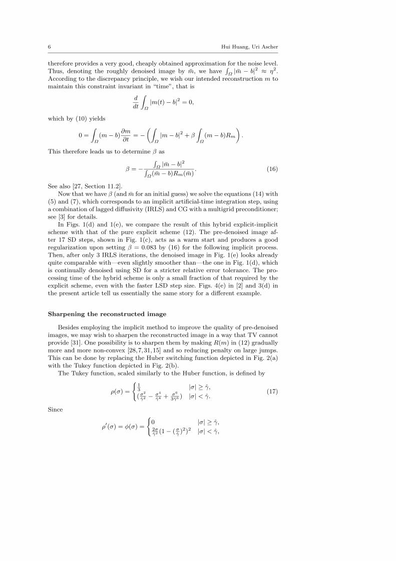
6 Hui Huang, Uri Ascher
therefore provides a very good, cheaply obtained approximation for the noise level.Thus, denoting the roughly denoised image by m, we have
∫Ω|m − b|2 ≈ η2.
According to the discrepancy principle, we wish our intended reconstruction m tomaintain this constraint invariant in “time”, that is
d
dt
∫Ω
|m(t)− b|2 = 0,
which by (10) yields
0 =
∫Ω
(m− b)∂m∂t
= −(∫
Ω
|m− b|2 + β
∫Ω
(m− b)Rm).
This therefore leads us to determine β as
β = −∫Ω|m− b|2∫
Ω(m− b)Rm(m)
. (16)
See also [27, Section 11.2].Now that we have β (and m for an initial guess) we solve the equations (14) with
(5) and (7), which corresponds to an implicit artificial-time integration step, usinga combination of lagged diffusivity (IRLS) and CG with a multigrid preconditioner;see [3] for details.
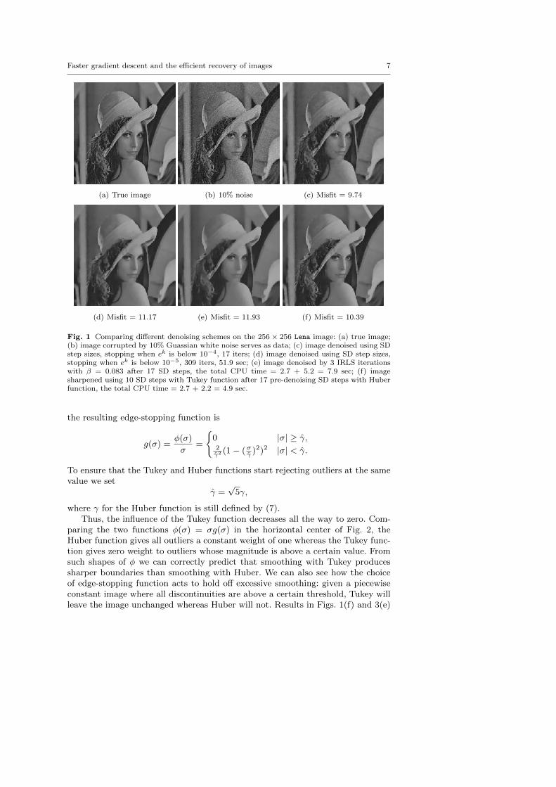
In Figs. 1(d) and 1(e), we compare the result of this hybrid explicit-implicitscheme with that of the pure explicit scheme (12). The pre-denoised image af-ter 17 SD steps, shown in Fig. 1(c), acts as a warm start and produces a goodregularization upon setting β = 0.083 by (16) for the following implicit process.Then, after only 3 IRLS iterations, the denoised image in Fig. 1(e) looks alreadyquite comparable with—even slightly smoother than—the one in Fig. 1(d), whichis continually denoised using SD for a stricter relative error tolerance. The pro-cessing time of the hybrid scheme is only a small fraction of that required by theexplicit scheme, even with the faster LSD step size. Figs. 4(e) in [2] and 3(d) inthe present article tell us essentially the same story for a different example.
Sharpening the reconstructed image
Besides employing the implicit method to improve the quality of pre-denoisedimages, we may wish to sharpen the reconstructed image in a way that TV cannotprovide [31]. One possibility is to sharpen them by making R(m) in (12) graduallymore and more non-convex [28,7,31,15] and so reducing penalty on large jumps.This can be done by replacing the Huber switching function depicted in Fig. 2(a)with the Tukey function depicted in Fig. 2(b).
The Tukey function, scaled similarly to the Huber function, is defined by
ρ(σ) =
13 |σ| ≥ γ,(σ
2
γ2 − σ4
γ4 + σ6
3γ6 ) |σ| < γ.(17)
Since
ρ′(σ) = φ(σ) =
0 |σ| ≥ γ,2σγ2 (1− (σγ )2)2 |σ| < γ,
Faster gradient descent and the efficient recovery of images 7
(a) True image (b) 10% noise (c) Misfit = 9.74
(d) Misfit = 11.17 (e) Misfit = 11.93 (f) Misfit = 10.39
Fig. 1 Comparing different denoising schemes on the 256 × 256 Lena image: (a) true image;(b) image corrupted by 10% Guassian white noise serves as data; (c) image denoised using SDstep sizes, stopping when ek is below 10−4, 17 iters; (d) image denoised using SD step sizes,stopping when ek is below 10−5, 309 iters, 51.9 sec; (e) image denoised by 3 IRLS iterationswith β = 0.083 after 17 SD steps, the total CPU time = 2.7 + 5.2 = 7.9 sec; (f) imagesharpened using 10 SD steps with Tukey function after 17 pre-denoising SD steps with Huberfunction, the total CPU time = 2.7 + 2.2 = 4.9 sec.
the resulting edge-stopping function is
g(σ) =φ(σ)
σ=
0 |σ| ≥ γ,2γ2 (1− (σγ )2)2 |σ| < γ.
To ensure that the Tukey and Huber functions start rejecting outliers at the samevalue we set
γ =√
5γ,
where γ for the Huber function is still defined by (7).Thus, the influence of the Tukey function decreases all the way to zero. Com-
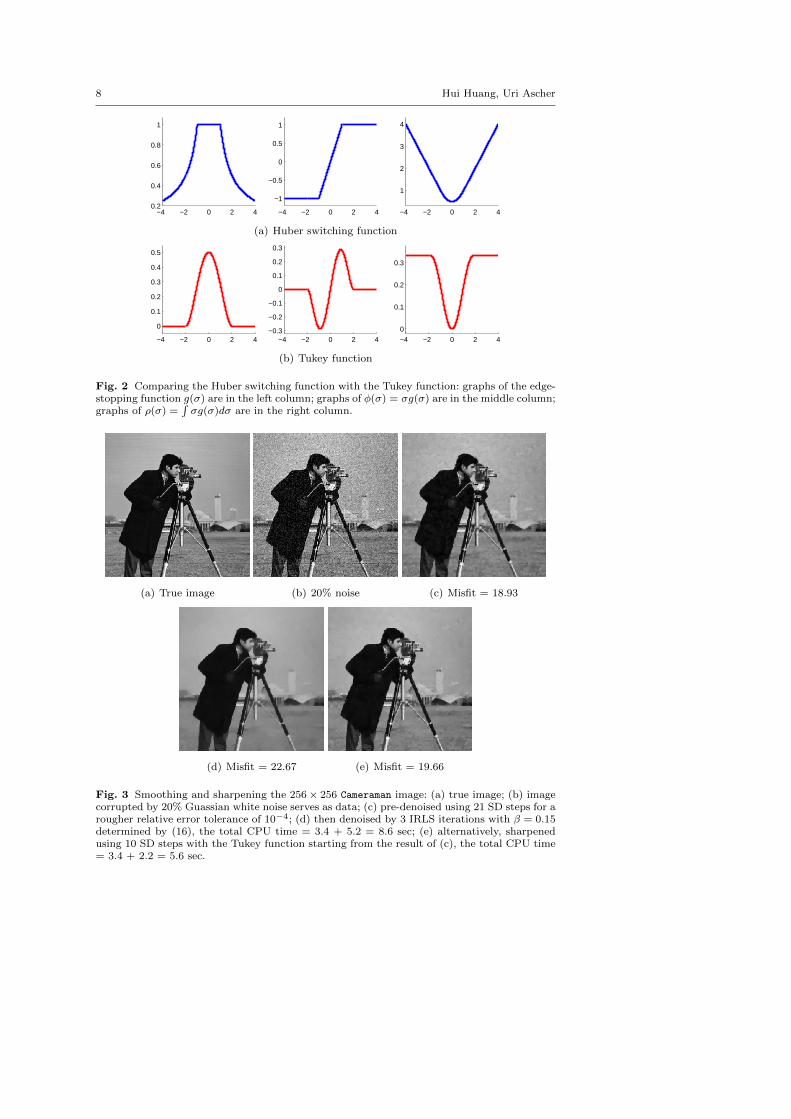
paring the two functions φ(σ) = σg(σ) in the horizontal center of Fig. 2, theHuber function gives all outliers a constant weight of one whereas the Tukey func-tion gives zero weight to outliers whose magnitude is above a certain value. Fromsuch shapes of φ we can correctly predict that smoothing with Tukey producessharper boundaries than smoothing with Huber. We can also see how the choiceof edge-stopping function acts to hold off excessive smoothing: given a piecewiseconstant image where all discontinuities are above a certain threshold, Tukey willleave the image unchanged whereas Huber will not. Results in Figs. 1(f) and 3(e)
8 Hui Huang, Uri Ascher
−4 −2 0 2 40.2
0.4
0.6
0.8
1
−4 −2 0 2 4
−1
−0.5
0
0.5
1
−4 −2 0 2 4
1
2
3
4
(a) Huber switching function
−4 −2 0 2 4
0
0.1
0.2
0.3
0.4
0.5
−4 −2 0 2 4−0.3
−0.2
−0.1
0
0.1
0.2
0.3
−4 −2 0 2 4
0
0.1
0.2
0.3
(b) Tukey function
Fig. 2 Comparing the Huber switching function with the Tukey function: graphs of the edge-stopping function g(σ) are in the left column; graphs of φ(σ) = σg(σ) are in the middle column;graphs of ρ(σ) =
∫σg(σ)dσ are in the right column.
(a) True image (b) 20% noise (c) Misfit = 18.93
(d) Misfit = 22.67 (e) Misfit = 19.66
Fig. 3 Smoothing and sharpening the 256 × 256 Cameraman image: (a) true image; (b) imagecorrupted by 20% Guassian white noise serves as data; (c) pre-denoised using 21 SD steps for arougher relative error tolerance of 10−4; (d) then denoised by 3 IRLS iterations with β = 0.15determined by (16), the total CPU time = 3.4 + 5.2 = 8.6 sec; (e) alternatively, sharpenedusing 10 SD steps with the Tukey function starting from the result of (c), the total CPU time= 3.4 + 2.2 = 5.6 sec.

Faster gradient descent and the efficient recovery of images 9
confirm our predictions. After a quick pre-denoising with Huber, only 10 SD stepswith Tukey result in obviously sharper discontinuities, i.e., image edges, than thosewithout switching the regularization operator; see Figs. 1 and 3.
It is important to note that a rough pre-denoising is necessary here. It helps usavoid strengthening undesirable effects of heavy noise by using the Tukey function.
From an experimental point of view, we recommend to apply the explicit-implicit LSD scheme if a smooth image is desired; otherwise, employ the explicitTukey regularization, starting from the result of the rough explicit Huber regular-ization, to get a sharper version.
3 Deblurring
Here we consider the deblurring problem discussed in [33,10,22]. The blurring ofan image can be caused by many factors: (i) movement during the image captureprocess, by the camera or, when long exposure times are used, by the subject; (ii)out-of-focus optics, use of a wide-angle lens, atmospheric turbulence, or a shortexposure time, which reduces the number of photons captured; (iii) scattered lightdistortion in confocal microscopy. Mathematically, in most cases blurring can belinearly modeled to be shift-invariant with a point spread function (PSF), denotedby f(x, y). Further, it is well known in signal processing and systems theory [25,26]that a shift-invariant linear operator must be in the form of convolution, writtenas
F (m) = f(x, y) ∗m(x, y) =
∫R2
f(x− x′, y − y′)m(x′, y′)dx′dy′. (18)
So, an observed blurred image b is related to the ideal sharp image m(x, y) by
b = f(x, y) ∗m(x, y) + ε,
where ∗ denotes convolution product and the point spread function f(x, y) mayvary in space. Thus, the matrix-vector multiplication Jm represents a discretemodel of the distortion operator (18) convolved by the PSF.
In the spatial domain, the PSF describes the degree to which an optical systemblurs or spreads a point of light. The PSF is the inverse Fourier transform of theoptical transfer function (OTF). In the frequency domain, the OTF describes theresponse of a linear, position-invariant system to an impulse. The distortion iscreated by convolving the PSF with the original true image, see [33,10]. Note thatdistortion caused by a PSF is just one type of data degradation, and the clearimage mtrue generally does not exist in reality. This image represents the resultof perfect image acquisition conditions. Nonetheless, in our numerical experimentswe have a “ground truth” model mtrue which is used to synthesize data and judgethe quality of reconstructions.
In the implementation we apply the same discretization as in Chapter 5 of [33],and then the convolution (18) is discretized into a matrix-vector multiplication,yielding a problem of the form (1), (2), where J is an N ×N symmetric, doublyblock Toeplitz matrix. Such a blurring matrix J can be constructed by a Kro-necker product. However, J is now a full, large matrix, and avoiding its explicitconstruction and storage is therefore desirable. Using a gradient descent algorithm

10 Hui Huang, Uri Ascher
we actually only need two matrix-vector products to form JT (Jm), and there isno reason to construct or store the matrix J itself. Moreover, it is possible to usea 2D fast Fourier transform (FFT) algorithm to reduce the computational cost ofthe relevant matrix-vector multiplication from O(N2) to O(N logN). Specifically,after discretizing the integral operator (18) in the form of convolution, we have afully discrete model
bi,j =n∑p=0
n∑q=0
fi−p,j−qmp,q + εi,j , 0 ≤ i, j ≤ n,
where εi,j denotes random noise at the grid location (i, j). In general, the discretePSF fi,jni,j=0 is 2D-periodic, defined as
fi,j = f(i′, j), whenever i = i′ mod n+ 1,
fi,j = f(i, j′), whenever j = j′ mod n+ 1.
This suggests we only need consider f ∈ R(n+1)×(n+1), because by periodic exten-sion we can easily get (n+ 1, n+ 1)-periodic arrays fext, for which
fexti,j = fi,j , whenever 0 ≤ i, j ≤ n.
Then the FFT algorithm yields
fext ∗m = (n+ 1)F−1F(f) . ∗ F(m),
where F is the discrete Fourier transform and .∗ denotes component-wise multi-plication.
Thus, we consider the gradient descent algorithm (9), starting from the datam0 = b, and compare the step size choices (11a) vs. (11b). As before, strictlyspeaking, these would be steepest descent and lagged steepest descent only ifL defined in (6) were constant, i.e., using least-squares regularization. But weproceed to freeze L for this purpose anyway, which amounts to a lagged diffusivityapproach.
One difference from the denoising problem is that here we do not have aneasy tool for determining the regularization parameter β, and it is determinedexperimentally instead. However, for the problems discussed below this turns outnot to be a daunting task.
To illustrate and analyze our deblurring algorithm, we generate some degradeddata at first. We use the Matlab function fspecial to create a variety of correla-tion kernels, i.e., PSFs, and then deliberately blur clear images by convolving themwith these different PSFs. The function fspecial(type,parameters) accepts afilter type plus additional modifying parameters particular to the type of filter cho-sen. Thus, fspecial(‘motion’,len,theta) returns a filter to approximate, onceconvolved with an image, the linear motion of a camera by len pixels with an angleof theta degrees in a counterclockwise direction, which therefore becomes a vec-tor for horizontal and vertical motions (see Fig. 4); fspecial(‘log’,hsize,sigma)returns a rotationally symmetric Laplacian of Gaussian filter of size hsize withstandard deviation sigma (see Fig. 6); fspecial(‘disk’,radius) returns a circu-lar mean filter within the square matrix of side 2radius+1 (see Fig. 7); fspe-cial(‘unsharp’,alpha) returns a 3×3 unsharp contrast enhancement filter, which

Faster gradient descent and the efficient recovery of images 11
(a) True image (b) motion blur
(c) β = 10−3, 23 LSD iters (d) β = 10−4, 33 LSD iters (e) β = 10−5, 38 LSD iters
Fig. 4 type = ‘motion’, len = 15, theta = 30, η = 1.
0 5 10 15 20 250
0.5
1
1.5
2
(a) SD − τ β = 10−3
0 5 10 15 20 250
1
2
3
4
(c) LSD − τ β = 10−30 5 10 15 20 25 30 35
0
10
20
30
(d) LSD − τ β = 10−4
0 20 40 60 80 1001
1.5
2
2.5
3
3.5
(b) SD − τ β = 10−4
Fig. 5 SD step size (11a) vs. LSD step size (11b) for the deblurring example in Fig. 4 underthe relative error tolerance of 10−4: (a) and (c) compare SD with LSD for β = 10−3, 25 SDiters vs. 23 LSD iters; (b) and (d) compare them for β = 10−4, 113 SD iters vs. 33 LSD iters.Note the horizontal scale (number of iterations) difference between (b) and (d).

12 Hui Huang, Uri Ascher
(a) True image (b) log blur (c) 114 SD or 31 LSD iters
Fig. 6 type = ‘log’, hsize = [512, 512], sigma = 0.5, η = 1, β = 10−4.
(a) True image (b) disk blur (c) 99 SD or 26 LSD iters
Fig. 7 type = ‘disk’, radius = 5, η = 1, β = 10−4.
(a) True image (b) unsharp blur (c) 17 SD or 15 LSD iters
Fig. 8 type = ‘unsharp’, alpha = 0.2, η = 1, β = 10−4.
enhances edges and other high frequency components by subtracting a smoothedunsharp version of an image from the original image, and the shape of which is con-trolled by the parameter alpha (see Fig. 8); fspecial(‘gaussian’,hsize,sigma)returns a rotationally symmetric Gaussian low-pass filter of size hsize with stan-dard deviation sigma (see Fig. 9); fspecial(‘laplacian’,alpha) returns a 3× 3filter approximating the shape of the two-dimensional Laplacian operator and theparameter alpha controls the shape of the Laplacian (see Fig. 10).
Faster gradient descent and the efficient recovery of images 13
All six images presented and used in this section are 256×256. For the first fourexperiments, we only add a small amount of random noise into blurred images, say1% (η = 1), and stop deblurring when the relative error norm (13) is below 10−4.For a given PSF, the only parameter required is the regularization parameter β.From Fig. 4 we can clearly see that the smaller β is, the sharper the restoredsolution is, including both image and noise. So the Boat image reconstructed withβ = 10−3 in Fig. 4(c) still looks blurry and that cannot be improved by runningmore iterations. The Boat image deblurred with β = 10−5 in Fig. 4(e) becomesmuch clearer; however, unfortunately, such a small β also brings the undesirableeffect of noise amplification. The setting β = 10−4 seems to generate the bestapproximation of the original scene, and so it does in the following three deblurringexperiments.
As in the case of denoising, the LSD step size selection (11b) usually yieldsfaster convergence than SD. When β is small, e.g., 10−4 or less, the step size (11a)is very close to the strict steepest descent selection obtained for a constant L, andso the famous two-periodic cycle of [1] (see also [2]) appears in the step sequence,resulting in a rather slow convergence; see Fig. 5(b). The lagged step size (11b)breaks this cycling pattern (see Fig. 5(d)), providing a much faster convergence forthe same error tolerance. Moreover, with the same parameter β, the reconstructedimages using both SD and LSD are quite comparable, and it is difficult to tellany differences between them by the naked eye. For β = 10−5, 335 SD steps arerequired to reach a result comparable to Fig. 4(e) and the corresponding CPUtime is 441.6 sec. Using LSD we only need 48.7 sec, reflecting the fact that theCPU time is roughly proportional to the number of steps required.
Figs. 6 – 8 reinforce our previous observations that the gradient descent de-blurring algorithm with LSD step selection (11b) works very well, and that theimprovement of LSD over SD is even more significant here than in the case of de-noising. This is especially pronounced when a small value of β must be chosen andwhen accuracy considerations require more than 20 or so steepest descent steps.
In [2] we have discussed other faster gradient descent methods. The half-laggedsteepest descent (HLSD) method [29,19] was generally found there to consistentlybe at par with LSD, while other variants performed somewhat worse. In the presentarticle we have applied HLSD in place of LSD for the above four examples, wherethe step size selection counts most. With HLSD the formula (11a) is applied only ateach even-numbered step and then the same step size gets reused in the followingodd-numbered one. The results were found to be again comparable to those usingLSD, both in terms of efficiency and in terms of quality.
We have also experimented with a version of CG where we locally pretend, asin (11), that the minimization problem is quadratic. However, the CG method iswell-known to be more sensitive than gradient descent to violations of its premises,and its iteration counts when applied to each of the examples in Figs. 4 – 7 wereconsistently about 20% higher than the better of LSD and HLSD.
Deblurring noisier images
The operation of deblurring essentially sharpens the image, whereas denoisingessentially smooths it. Thus, trouble awaits any algorithm when both significantblur and significant noise are present in the given data set.

14 Hui Huang, Uri Ascher
(a) True image (b) gaussian blur (c) Noise amplification
(d) Pre-denoised (e) Deblurred (f) Sharpened
Fig. 9 type = ‘gaussian’, hsize = [512, 512], sigma = 1.5: (b) data b corresponding toη = 5; (c) directly deblurring using β = 5× 10⁻⁴ fails; (d) pre-denoising: for the relative errortolerance of 10−4, 9 LSD steps of (12) are required; (e) 22 steps of (9) with β = 5 × 10⁻⁴
and LSD (11b) are required for the next deblurring; (f) 10 sharpening steps with the Tukeyfunction (17) follow. The total CPU time = 16.1 sec.
In our present setting, if we add more noise to the blurred images when synthe-sizing the data, say η ≥ 5, then directly running the deblurring gradient descentalgorithm as above may fail due to the more severe effect of noise amplification;see, e.g., Figs. 9(c) and 10(c). After a few iterations, the restored image can havea speckled appearance, especially for a smooth object observed at low signal-to-noise ratios. These speckles do not represent any real texture in the image, butare artifacts of fitting the noise in the given image too closely. Noise amplificationcan be reduced by increasing the value of β, but this may result in a still blurryimage, as in Fig. 4(c). Since the effects of noise and blur are opposite, a quick andto some extent effective remedy is splitting, described next.
At first, we only employ denoising up to a coarser tolerance, e.g., 10−4. Thiscan be carried out in just a few steps of (12) with either the SD or LSD stepsize selection. Starting with the lightly denoised image, as in Figs. 9(d) and 10(d),we next apply the deblurring algorithm (9) with the LSD step sizes to correctPSF distortion. Since now the noise level becomes higher, we slightly increase thevalue of the regularization parameter and apply β = 5×10⁻⁴ for the Toy exampleand β = 10−3 for the Pepper example. Observe that, even though some specklesstill appear on the image cartoon components, the results presented in Figs. 9(e)and 10(e) are much more acceptable than those in Figs. 9(c) and 10(c), whichwere deblurred by the same number of iterations without pre-denoising. Finally,

Faster gradient descent and the efficient recovery of images 15
(a) True image (b) laplacian blur (c) Noise amplification
(d) Pre-denoised (e) Deblurred (f) Sharpened
Fig. 10 type = ‘Laplacian’, alpha = 0.2: (b) data b corresponding to η = 10; (c) directlydeblurring using β = 10−3 fails; (d) pre-denoising: for the relative error tolerance of 10−4, 10LSD steps of (12) are required; (e) 25 steps of (9) with β = 10−3 and LSD (11b) are requiredfor the next deblurring; (f) 10 sharpening steps with the Tukey function (17) follow. The totalCPU time = 14.5 sec.
we can use the Tukey regularization in (12) to further improve the reconstruction,carefully yet rapidly removing unsuitable speckles and enhancing the contrast, i.e.,sharpening. The results are demonstrated in Figs. 9(f) and 10(f). The total CPUtime, given in the captions of Figs. 9 and 10, clearly shows the efficiency of thishybrid deblurring-denoising scheme.
4 Conclusions
In this paper we have examined the effect of replacing steepest descent (SD) bya faster gradient descent algorithm, specifically, lagged steepest descent (LSD), inthe practical context of image deblurring and denoising tasks. We have also pro-posed several highly efficient schemes for carrying out these tasks, independentlyof the step size selection.
Our general conclusion is that in situations where many (say, over 20) steepestdescent steps are required, thus building slowness into the solution procedure, thefaster gradient descent method offers substantial advantages.
Specifically, four scenarios have been considered. The first is a straightforwarddenoising process using anisotropic diffusion [2]. Here the LSD step selection offersan efficiency improvement by a factor of roughly 3.

16 Hui Huang, Uri Ascher
In contrast, the second denoising scenario does not allow slowness buildup bySD because after a quick rough denoising we switch to an implicit method, witha good estimate for β at hand, or to a sharpening phase using (17). The resultingmethod is new and effective, although not because of a dose of LSD.
Switching to the more interesting and challenging deblurring problem, the thirdscenario envisions the presence of little additional noise, so we directly employ thegradient descent method (9) with J as described in Section 3, R given by (5) and(7), and β = 10−4. This allows for slowness buildup when using SD step sizes, andthe faster LSD variant then excels, becoming up to 10 times more efficient. TheHLSD variant is overall as effective as LSD.
Finally, in the presence of significant noise effective deblurring becomes aharder task. We propose a splitting approach whereby we switch between thepreviously developed denoising and deblurring algorithms. This again creates asituation where LSD does not contribute much improvement over SD. The split-ting approach has been demonstrated to be relatively effective, although none ofthe reconstructions in Fig. 10, for instance, is amazingly good. The problem itselfcan become very hard to solve satisfactorily, unless some rather specific knowl-edge about the noise is available and can be used to carefully remove it beforedeblurring begins.
A future problem to be considered concerns the case where the PSF causingblurring is not known.
References
1. Akaike, H.: On a successive transformation of probability distribution and its applicationto the analysis of the optimum gradient method. Ann. Inst. Stat. Math. Tokyo 11, 1–16(1959)
2. Ascher, U., Doel, K.v.d., Huang, H., Svaiter, B.: Gradient descent and fast artificial timeintegration. M2AN 43, 689–708 (2009)
3. Ascher, U., Haber, E., Huang, H.: On effective methods for implicit piecewise smoothsurface recovery. SIAM J. Sci. Comput. 28, 339–358 (2006)
4. Ascher, U., Huang, H., Doel, K.v.d.: Artificial time integration. BIT 47, 3–25 (2007)5. Barzilai, J., Borwein, J.: Two point step size gradient methods. IMA J. Num. Anal. 8,
141–148 (1988)6. Berg, E.v.d., Friedlander, M.: Probing the Pareto frontier for basis pursuit solutions. SIAM
J. Scient. Comput. 31, 890–912 (2008)7. Black, M.J., Sapiro, G., Marimont, D.H., Heeger, D.: Robust anisotropic diffusion. IEEE
trans. image processing 7(3), 421–432 (1998)8. Calvetti, D., Reichel, L.: Lanczos-based exponential filtering for discrete ill-posed prob-
lems. Numer. Algorithms 29, 45–65 (2002)9. Chan, T., Mulet, P.: On the convergence of the lagged diffusivity fixed point method in
total variation image restoration. SIAM J. Numer. Anal. 36, 354–367 (1999)10. Chan, T., Shen, J.: Image Processing and Analysis: Variational, PDE, Wavelet and
Stochastic Methods. SIAM (2005)11. Claerbout, J., Muir, F.: Robust modeling with erratic data. Geophysics 38, 826–844 (1973)12. Dai, Y., Fletcher, R.: Projected Barzilai-Borwein methods for large-scale box-constrained
quadratic programming. Numerische. Math. 100, 21–47 (2005)13. Daubechies, I., de Friese, M., de Mol, C.: An iterative thresholding algorithm for linear
inverse problems with sparsity constraints. Comm. Pure Appl. Math 57, 1413–1457 (2004)14. Doel, K.v.d., Ascher, U.: The chaotic nature of faster gradient descent methods. J. Scient.
Comput. DOI10.1007/s10915-011-9521-3 (2011)15. Durand, F., Dorsey, J.: Fast bilateral filtering for the display of high-dynamic-range images.
ACM Trans. Graphics (SIGGRAPH) 21(3), 257–266 (2002)16. Engl, H.W., Hanke, M., Neubauer, A.: Regularization of Inverse Problems. Kluwer (1996)

Faster gradient descent and the efficient recovery of images 17
17. Farquharson, C., Oldenburg, D.: Non-linear inversion using general measures of data misfitand model structure. Geophysics J. 134, 213–227 (1998)
18. Figueiredo, M., Nowak, R., Wright, S.: Gradient projection for sparse reconstruction: ap-plication to compressed sensing and other inverse problems. IEEE J. Special Topics onSignal Processing 1, 586–598 (2007)
19. Friedlander, A., Martinez, J., Molina, B., Raydan, M.: Gradient method with retard andgeneralizations. SIAM J. Num. Anal. 36, 275–289 (1999)
20. Gilyazov, S., Gol’dman, N.: Regularization of Ill-Posed Problems by Iterative Methods.Kluwer (2000)
21. Hansen, P.C.: Rank Deficient and Ill-Posed Problems. SIAM, Philadelphia (1998)22. Hardy, J.W.: Adaptive Optics for Astronomical Telescopes. Oxford University Press, NY
(1998)23. Mallat, S.: A Wavelet Tour of Signal Processing: the Sparse Way. Academic Press (2009).
3rd Ed.24. Nocedal, J., Sartenar, A., Zhu, C.: On the behavior of the gradient norm in the steepest
descent method. Comput. Optim. Appl. 22, 5–35 (2002)25. Oppenheim, A.V., Schafer, R.W.: Discrete-Time Signal Precessing. Prentice-Hall, Enge-
wood Cliffs, NJ (1989)26. Oppenheim, A.V., Willsky, A.S.: Signals and Systems. Prentice-Hall, Engewood Cliffs, NJ
(1996)27. Osher, S., Fedkiw, R.: Level Set Methods and Dynamic Implicit Surfaces. Springer (2003)28. Perona, P., Malik, J.: Scale-space and edge detection using anisotropic diffusion. IEEE
Transactions on Pattern Analysis and Machine Intelligence 12(7), 629–639 (1990)29. Raydan, M., Svaiter, B.: Relaxed steepest descent and Cauchy-Barzilai-Borwein method.
Comput. Optim. Appl. 21, 155–167 (2002)30. Rudin, L., Osher, S., Fatemi, E.: Nonlinear total variation based noise removal algorithms.
Physica D 60, 259–268 (1992)31. Sapiro, G.: Geometric Partial Differential Equations and Image Analysis. Cambridge
(2001)32. Tikhonov, A.N., Arsenin, V.Y.: Methods for Solving Ill-posed Problems. John Wiley and
Sons, Inc. (1977)33. Vogel, C.: Computational methods for inverse problem. SIAM, Philadelphia (2002)
![Stochastic Gradient Descent Tricks - bottou.org2.1 Gradient descent It has often been proposed (e.g., [18]) to minimize the empirical risk E n(f w) using gradient descent (GD). Each](https://img.pdfslide.net/doc/110x75/60bec0701f04811115495619/stochastic-gradient-descent-tricks-21-gradient-descent-it-has-often-been-proposed.jpg)