Fate of Volatile Chemicals during Accretion on Wet-Growing

University of South FloridaScholar Commons

Graduate Theses and Dissertations Graduate School

7-17-2008

Fate of Volatile Chemicals during Accretion onWet-Growing HailRyan A. MichaelUniversity of South Florida

Follow this and additional works at: https://scholarcommons.usf.edu/etd

Part of the American Studies Commons

This Thesis is brought to you for free and open access by the Graduate School at Scholar Commons. It has been accepted for inclusion in GraduateTheses and Dissertations by an authorized administrator of Scholar Commons. For more information, please contact [email protected].

Scholar Commons CitationMichael, Ryan A., "Fate of Volatile Chemicals during Accretion on Wet-Growing Hail" (2008). Graduate Theses and Dissertations.https://scholarcommons.usf.edu/etd/406

http://scholarcommons.usf.edu/?utm_source=scholarcommons.usf.edu%2Fetd%2F406&utm_medium=PDF&utm_campaign=PDFCoverPages

http://scholarcommons.usf.edu/?utm_source=scholarcommons.usf.edu%2Fetd%2F406&utm_medium=PDF&utm_campaign=PDFCoverPages

https://scholarcommons.usf.edu?utm_source=scholarcommons.usf.edu%2Fetd%2F406&utm_medium=PDF&utm_campaign=PDFCoverPages

https://scholarcommons.usf.edu/etd?utm_source=scholarcommons.usf.edu%2Fetd%2F406&utm_medium=PDF&utm_campaign=PDFCoverPages

https://scholarcommons.usf.edu/grad?utm_source=scholarcommons.usf.edu%2Fetd%2F406&utm_medium=PDF&utm_campaign=PDFCoverPages

https://scholarcommons.usf.edu/etd?utm_source=scholarcommons.usf.edu%2Fetd%2F406&utm_medium=PDF&utm_campaign=PDFCoverPages

http://network.bepress.com/hgg/discipline/439?utm_source=scholarcommons.usf.edu%2Fetd%2F406&utm_medium=PDF&utm_campaign=PDFCoverPages

mailto:[email protected]

Fate of Volatile Chemicals during Accretion on Wet-Growing Hail

by

Ryan A. Michael

A thesis submitted in partial fulfillment of the requirements for the degree of

Master of Science in Engineering Science Department of Civil and Environmental Engineering

College of Engineering University of South Florida

Major Professor: Amy L. Stuart, Ph.D. Jeffrey Cunningham, Ph.D. Jennifer M. Collins, Ph.D.

Maya A. Trotz, Ph.D.

Date of Approval: July 17, 2008

Keywords: atmospheric chemistry, riming, retention, ice microphysics, cloud modeling

© Copyright 2008 , Ryan A. Michael

Acknowledgements

This thesis would not have been successfully completed without the help of many

people to whom I am grateful and because of whom my experience has been

unforgettable.

First, I wish to convey my thanks to my advisor, Amy Stuart, for making this

feasible. From providing funds to instilling knowledge, your support throughout my

study has been paramount to my success. Thank you for holding me to such high

standards with your perceptive remarks and constructive criticisms at every stage of my

research. More importantly, thank you for your patience, for sticking with me when even

I wanted to throw my hands up.

I thank the members of my thesis committee, Maya Trotz, Jennifer Collins, and

Jeffrey Cunningham. Thank you for your meticulous reviews. Your insightful comments

were instrumental in helping to shape this work.

I am forever grateful to the late Calvin Miller who did not give me life but gave

me the life I have. Thank you for believing in me, you are forever in my thoughts.

I would like to express my gratitude to the following persons for their help

throughout this process: Chris Einmo, Monica Gray, Roland Okwen, Edolla Prince, Luis

Baluto Torrez, and Nicole Watson

To my loving mother, Adnic West, to whom this thesis is dedicated, I say thank

you. I am most indebted to you for your inestimable help, limitless sacrifices, and

unconditional love throughout my life. Without you, this would not have been possible.

i

Table of Contents

List of Tables ..................................................................................................................... iii

List of Figures .................................................................................................................... iv

ABSTRACT ........................................................................................................................ v

1. Introduction ................................................................................................................... 1

1.1. Background .................................................................................................... 1

1.2. Convective cloud systems .............................................................................. 1

1.3. Cloud hydrometeors and chemical interactions ............................................. 3

1.4. Ice-chemical interactions ............................................................................... 5

1.5. Thesis organization ........................................................................................ 7

2. Model Development ..................................................................................................... 9

2.1. Retention ratio ................................................................................................ 9

2.2. Microphysical process variables .................................................................. 13

2.3. Model parameters and assumptions ............................................................. 15

2.4. Implementation ............................................................................................ 18

2.5. Testing.......................................................................................................... 26

3. Application .................................................................................................................. 28

4. Results ......................................................................................................................... 29

4.1. Hail factors ................................................................................................... 29

4.1.1. Hail diameter ..................................................................................... 29

ii

4.1.2. Mass fraction liquid water content of hail ......................................... 34

4.1.3. Ice-liquid interface temperature ........................................................ 35

4.1.4. Hail shape factor ................................................................................ 36

4.1.5. Efficiency of collection ..................................................................... 37

4.2. Environmental factors .................................................................................. 38

4.2.1. Cloud liquid water content ................................................................ 38

4.2.2. Drop radius ........................................................................................ 39

4.2.3. Pressure ............................................................................................. 42

4.2.4. Air temperature .................................................................................. 43

4.3. Chemical factors .......................................................................................... 45

4.3.1. Chemical effective Henry’s constant and pH .................................... 45

4.3.2. The effective ice-liquid distribution coefficient ................................ 48

4.4. Summary of results ...................................................................................... 49

5. Discussion and Limitations ......................................................................................... 51

6. Conclusions and Implications ..................................................................................... 56

7. List of References ....................................................................................................... 58

Appendices ........................................................................................................................ 71

Appendix A. Retention Model Calculations ......................................................... 72

About the Author ................................................................................................... End Page

iii

List of Tables

Table 1. Methods for estimation of model parameters ..................................................... 16

Table 2. Chemical properties and thermodynamic data.................................................... 21

Table 3. Model input variables and ranges ....................................................................... 23

Table 4. Dependence of simulated retention fraction on input variables ......................... 50

Table A. Retention model calculations ............................................................................. 72

iv

List of Figures

Figure 1. Hail growth and solute transfer processes. ........................................................ 10

Figure 2. The effect of individual hail input variables on retention fraction.. .................. 31

Figure 3. The effect of individual hail input variables on the growth rate boundary

parameter, GB. ................................................................................................. 32

Figure 4. The effect of individual hail input variables on the wet growth boundary

parameter, WB. ................................................................................................. 33

Figure 5. The effect of individual environmental input variables on the retention

fraction. ............................................................................................................. 41

Figure 6. The effect of individual environmental input variables on the growth rate

boundary parameter, GB. ................................................................................. 41

Figure 7. The effect of individual environmental input variables on the wet growth

boundary parameter, WB. ................................................................................ 42

Figure 8. The effect of individual chemical input variables on the retention fraction. ..... 47

Figure 9. The effect of individual chemical input variables on the growth rate

boundary parameter, GB. ................................................................................. 47

Figure 10. The effect of individual chemical input variables on the wet growth

boundary parameter, WB. ................................................................................ 48

v

Fate of Volatile Chemicals during Accretion on Wet-Growing Hail

Ryan Michael

ABSTRACT

Phase partitioning during freezing of hydrometeors affects the transport and

distribution of volatile chemical species in convective clouds. Here, the development,

evaluation, and application of a mechanistic model for the study and prediction of

partitioning of volatile chemical during steady-state hailstone growth are discussed. The

model estimates the fraction of a chemical species retained in a two-phase growing

hailstone. It is based upon mass rate balances over water and solute for constant accretion

under wet-growth conditions. Expressions for the calculation of model components,

including the rates of super-cooled drop collection, shedding, evaporation, and hail

growth were developed and implemented based on available cloud microphysics

literature. A modified Monte Carlo simulation approach was applied to assess the impact

of chemical, environmental, and hail specific input variables on the predicted retention

ratio for six atmospherically relevant volatile chemical species, namely, SO2, H2O2, NH3,

HNO3, CH2O, and HCOOH. Single input variables found to influence retention are the

ice-liquid interface supercooling, the mass fraction liquid water content of the hail, and

the chemical specific effective Henry’s constant (and therefore pH). The fraction retained

increased with increasing values of all these variables. Other single variables, such as hail

vi

diameter, shape factor, and collection efficiency were found to have negligible effect on

solute retention in the growing hail particle. The mean of separate ensemble simulations

of retention ratios was observed to vary between 1.0x10-8 and 1, whilst the overall range

for fixed values of individual input variables ranged from 9.0x10-7 to a high of 0.3. No

single variable was found to control these extremes, but rather they are due to

combinations of model input variables.

1

1. Introduction

1.1. Background

Knowledge of the upper tropospheric ozone budget is essential to our ability to

understand and predict climate change. Ozone concentrations in the troposphere are

regulated by catalytic cycles involving nitrogen oxides (NOx), hydrogen oxides (HOx),

and volatile organic carbon (VOC) species. In upper tropospheric regions influenced by

convection, the budget of NOx and the ratio of HOx to NOy (reactive nitrogen) are not

well understood, resulting in poorly understood ozone amounts [Jaeglé et al., 2001].

1.2. Convective cloud systems

The availability and concentration of ozone precursors in the troposphere are

significantly affected by the action of convective cloud systems. Convective cloud

systems significantly influence tropospheric chemistry and chemical deposition to the

ground by moving trace gas species from the boundary layer to the free troposphere

through chemical scavenging by cloud hydrometeors. Convective processing of trace gas

species is an important means of moving chemical constituents rapidly between the

boundary layer and free troposphere, and is an effective way of cleansing the atmosphere

through wet deposition. It also brings into the cloud, species that are of a different

composition, concentration, and origin than the air that ascends from the boundary layer

2

[Barth et al., 2002]. This entrained air can affect local thermodynamics as well as

chemical and microphysical processes.

Convective cloud systems have been shown to influence the chemical

characteristics of the upper troposphere to lower stratosphere region. They contribute to

the production, transportation, and redistribution of reactive chemical constituents,

including water, aerosols and long-lived tracers in the upper troposphere to lower

stratosphere [Dickerson et al., 1987; Gimson, 1997; Lelieveld and Crutzen, 1994; Ridley

et al., 2004; Yin et al., 2005]. These convective cloud systems can offer a rapid pathway

for the vertical transport of air containing reactive chemical species from the planetary

boundary layer to the upper troposphere [Barth et al., 2007; 2001]. Through

entrainment/detrainment processes, they can facilitate the mixing and dispersal of

pollutants, and the transport of reactive species over significantly shorter timescales than

would occur via eddy diffusion or other atmospheric mixing processes [Dickerson et al.,

1987]. At higher altitudes, increases in wind speed may result in longer atmospheric

residence times of chemical species, thus increasing the probability of their participation

in photochemical reactions and other atmospheric transformations [Ridley et al., 2004;

Stockwell et al., 1990; Rutledge et al., 1986]. Thus, convective cloud systems can be

thought of as chemical reactors, processing atmospheric air and its trace chemical

constituents.

However, the potential cleansing effect of deep convective cloud systems on the

atmospheric boundary layer is countered by negative impacts due to scavenging,

dissolution, and eventual deposition of acidic species. Effects of acid deposition may

include reduced buffering capacity of lakes and other surface water systems, forest

3

deaths, reduced visibility, material deterioration, and deleterious health effects such as

bronchitis and asthma [Cosby et al., 1985; Likens et al., 1996; Dockery et al., 1996].

Furthermore, venting of air from the atmospheric boundary layer by convective cloud

systems may influence tropospheric ozone concentrations due to the migration and

increased residence times of chemical species that regulates its production. These

processes may significantly affect the upper troposphere ozone budget, and consequently

climate change [Barth et al., 2002; Dickerson et al, 1987]. Additionally, as a result of

these strong convective processes, regional air pollution problems may be transformed to

global air pollution problems due to the long range transport of pollution plumes

[Dickerson et al, 1987]. Therefore, an understanding of the microphysical processes

governing the interaction of trace chemical species and condensed phase in convective

cloud system is imperative to our determination of their fate, and as understanding of

tropospheric ozone budget and climate change.

1.3. Cloud hydrometeors and chemical interactions

Previous studies have shown that the interaction of cloud hydrometeors with trace

chemical species may significantly influence the fate of these chemicals, and

subsequently impact atmospheric chemistry. Hydrometeors refer to the different forms of

condensed water that constitute convective clouds, and include ice crystals, snow,

graupel, and hail. Their formation is as a direct result of the moisture, temperatures,

pressures, and airflow conditions associated with convective cloud systems. These cloud

hydrometeors provide surfaces for chemical phase changes and reactions, act as

condensed-phase reactors, and serve as conduits for chemical transport from the

4

atmosphere to the ground, through scavenging and precipitation [Lamb and Blumenstein,

1987; Rutledge et al, 1986; Santachiara et al., 1995; Snider and Huang, 1998].

Interactions of volatile trace chemicals with cloud hydrometeors include absorption,

condensation, diffusion, vapor deposition, or incorporation into the growing hydrometeor

[Flossmann et al, 1985; 1987; Pruppacher and Klett, 1997]. Once dissolved in the

hydrometeor, depending on the characteristics of the phase, the trace chemicals may

dissociate or undergo further chemical reactions, thus affecting and modifying cloud and

atmospheric chemical distributions [Barth, 2000; 2001; 2007]. For example, the removal

of odd hydrogen species due to interactions with cloud hydrometeors has been found to

significantly affect the oxidizing capacity of the troposphere and contribute to increased

levels of sulfur species in precipitation [Audiffren et al, 1999; Snider, 1998].

Consequently, emphasis has been placed on understanding the interaction of trace

chemical species with hydrometeors in convective cloud systems through observational

and modeling studies. These include studies focusing on acid deposition [Barth et al.,

2000; Chameides, 1984; Daum et al., 1984; Kelly et al., 1985], ozone in the troposphere

[Lelieveld and Crutzen, 1994; Pickering et al., 1992; Prather and Jacob, 1997], and the

interaction of hydrometeors with other species [Chatfield and Crutzen 1984]. Most of the

models focused on liquid phase hydrometeors, and chemical species were distributed

based on processes governing liquid-phase exchanges. Consequently, little is known

about how microphysical processes involving ice affect chemical fate.

5

1.4. Ice-chemical interactions

Previous work indicates that ice-chemical interactions may have significant

impacts on cloud and atmospheric chemistry [Pruppacher and Klett, 1997; Stuart and

Jacobson, 2003; 2004; 2006]. Many researchers have included limited ice-chemical

interactions in cloud models [Audiffren et al., 1999; Chen and Lamb, 1994; Cho, 1989;

Rutledge et al., 1986]. Audiffren et al. [1999], in their two-dimensional Eulerian cloud

model, utilized the formulations of Lamb and Blumenstein [1987] and Iribarne and

Barrie [1950] in their parameterization of the entrapment of chemical species in a

growing ice-phase hydrometeor. Elucidation of the mechanism by which trace chemicals

and ice interact is important in order to predict chemical fate and to find suitable

parameterizations for larger scale modeling.

Recent studies indicate that one microphysical process, the freezing of super-

cooled drops via accretion, may significantly influence the venting of chemicals by

clouds [Yin et al., 2002, Barth et al., 2007; Cho et al., 1989]. Ice hydrometeors in

convective clouds may form and grow due to distinct microphysical transformations.

Three major categories of such transformations exist, delineated by specific

environmental conditions and giving rise to distinct hydrometer types [Pruppacher and

Klett, 1997]. These are non-rime freezing, dry-growth riming, and wet-growth riming.

Non-rime freezing involves the freezing of supercooled droplets without contact

with an already frozen substrate hydrometeor. This phenomenon is normally associated

with very low temperatures (< -30⁰C), and the associated ice nucleation may be either

homogeneous or heterogeneous in nature. Hydrometeors formed via this process

6

generally retain the approximate shape of the original supercooled drop [Hobbs, 1974;

Pruppacher an Klett, 1997].

Conversely, riming involves the collision and collection of supercooled water

drops by solid substrates, which may include, ice crystals, graupel, and hail, due to the

differences in velocity of the drops and substrate. Riming can be further classified into

either of two broad categories: wet-growth or dry growth riming. The regime a

hydrometeor grows in is greatly dependent on specific conditions of drop size,

hydrometeor speed, cloud water content, and temperatures (of air, drop, and riming

substrate). Wet-growth riming results in a partially frozen hydrometeor, which may

contain pockets of water in the hydrometer, or on the surface of the hydrometeor, and a

surface temperature of approximately 0⁰C. Due to these conditions, drop interference and

coalescence occurs, resulting in a more dense and transparent structure. Some liquid

water may be shed from the riming hydrometeor. Conversely, dry-growth riming is

associated with conditions of lower cloud water content and surface temperatures below

0⁰C. Due to the low temperatures associated, drop freezing occurs independently, without

coalescence, resulting in less dense, opaque hydrometeor. Because of the varying

environmental conditions and processes characterizing the different freezing categories,

factors affecting volatile chemicals retention in the frozen hydrometeor due to these

microphysical transformations may differ significantly.

Several authors have carried out laboratory studies investigating the degree to

which a volatile chemical species may be retained in the ice phase due to the riming

process. Consequently, they have characterized a retention ratio, which gives the ratio of

solute mass in the hydrometeor to that which was originally in the impinging droplet, i.e.,

7

the equilibrium concentration [Iribarne et al., 1983; Iribarne and Pyshnov, 1990; Lamb

and Blumenstein, 1987; Snider and Huang, 1998]. These investigations measured the

retention efficiencies of gases found in clouds including O2, SO2, H2O2, HNO3, HCl, and

NH3, and calculated values ranging between 0.01 and 1. Factors that varied among the

studies were summarized by Stuart and Jacobson [2003] and included temperature,

droplet and substrate size, solute concentration, pH, and impact speed.

To address the lack of understanding regarding the factors leading to the observed

differences in experimentally derived retention ratios, Stuart and Jacobson [2003; 2004;

2006] developed theory-based retention parameterizations and a mechanistic model under

conditions satisfying dry growth riming and non-rime freezing. The retention ratio was

found to be highly dependent on the effective Henry’s constant, drop velocity, and drop

size. The formation of a complete or partial ice shell was also found to have a significant

impact on retention. Chemicals with high effective Henry’s constant were found to be

completely retained. For those with negligible Henry’s constant values, retention was

found to be highly dependent on freezing conditions. However, the microphysical

processes determining volatile chemical fate during ice accretion in the wet-growth

regime remain poorly understood.

1.5. Thesis organization

In this study, I investigate the substrate properties, chemical characteristics, and

environmental variables affecting chemical retention under conditions of wet growth.

More specifically, this body of research attempts to answer the following scientific

questions:

8

• What chemical properties affect chemical retention in hail growing under wet-growth

conditions?

• What specific environmental conditions contribute to volatile chemical retention in

ice hydrometeors for conditions of wet growth?

• What particle-scale microphysical process influence volatile chemical retention for

accretion under wet growth conditions?

Stuart [2002] developed a mechanistic analytical equation for the evaluation of

volatile chemical retention during steady-state accretion on wet growing hail. The

derivation is presented again in Section 2.1, by permission of the author, for

completeness. In this thesis, I develop the expressions for microphysical process

variables (Section 2.2), and model parameters (Section 2.3) necessary to apply the model.

Model implementation and testing are discussed in Sections 2.4 and 2.5, respectively. It

is then applied (Section 3) to understand the likely dependence of partitioning on

environmental conditions and hail characteristics and chemical species. Results,

discussions, and conclusions are presented in Sections 4, 5, and 6, respectively.

9

2. Model Development

This model considers a two-phase (ice and liquid water) hail particle, growing at a

steady-rate, in a region of sufficiently high cloud liquid water content to satisfy

conditions for wet growth. Growth is facilitated by the collection of super-cooled water

drops in the volume swept out by the falling hail particle. The fate of solutes, originally

dissolved in the impinging drops, is determined by two coupled mass balances; a water

mass rate balance, and a solute mass balance over the growing hail particle. Expressions

describing the process governing hailstone development, such as impingement,

evaporation, and shedding, are derived from cloud microphysics.

2.1 Retention ratio

Wet growth is characterized by higher surface temperatures (~0⁰C), higher cloud

water mixing ratios, and higher rates of drop impingent on the substrate, than the

conditions associated with the dry-growth regime [Pruppacher and Klett, 1997, p. 659].

Under these conditions, impinging drops coalesce prior to freezing on the growing

hailstone. This may lead to the presence of a liquid water layer (skin) on the surface of

the hydrometeor and liquid water in entrapped pockets throughout the hailstone [Johnson

and Ramussen, 1992, Schumann, 1938]. If the skin is thick enough, water can be shed as

water droplets, due to gyration (rotation) of the hailstone [Garcia-Garcia and List, 1992].

Under wet-growth conditions, chemical solutes dissolved in the impacting drops

may be retained in the growing

entrapped in water pockets within hail

can be removed from the growing hail via shed water and through evaporation. Fig

illustrates the processes involved in solute

Under constant environmental conditions (temperatures,

content, and velocities), rates

growth will be approximately

partitioning will be at a constant rate

determining the salinity of sea spray ice, we can write a

during wet-growth:

10

growth conditions, chemical solutes dissolved in the impacting drops

may be retained in the growing hailstone, in the water film at the surface of the hail,

ntrapped in water pockets within hail ice, or incorporated in the ice structure

can be removed from the growing hail via shed water and through evaporation. Fig

illustrates the processes involved in solute retention during wet growth riming

Under constant environmental conditions (temperatures, pressure, cloud water

, rates of water flux to the hydrometeor, water shedding, and

approximately constant. Hence, hydrometeor growth and solute

a constant rate. Adapting the development of Makkonen

determining the salinity of sea spray ice, we can write a rate balance

ld h eX F X G X E X S= + +

Figure 1. Hail growth and solute transfer processes.

growth conditions, chemical solutes dissolved in the impacting drops

in the water film at the surface of the hail,

d in the ice structure. Solutes

can be removed from the growing hail via shed water and through evaporation. Figure 1

riming.

pressure, cloud water

of water flux to the hydrometeor, water shedding, and ice

hydrometeor growth and solute

Makkonen [1987] for

rate balance on solute mass

Eqn (1)

11

Here, F is the mass rate of drop collection, G is the mass rate of hydrometeor

growth, E is the mass rate of solution evaporation, and S is the mass rate of shedding,

each having units of mass per time. Xd, Xh, Xe, and Xl are the solute mass fractions, e.g.

gram solute per gram of solution, in the drops (d), evaporated solution (e), hydrometeor

(h), and surface (and shed) liquid (l). Note that this equation assumes that the liquid-to-

gas mass transfer (evaporation) rate for chemical solute is proportional to that for water

evaporation. This is a simplification for an open system (low concentrations of water

vapor and solute in the surrounding air), similar diffusivities in air, similar Schmidt

numbers, and equilibrium chemical partitioning at the liquid-gas interface.

It is noted that a water rate balance require S = F – E – G, and subsequent

rearrangement, results in the following:

( )

( ) ( )h lh

d h l e l

X X GX G

X F X X G X X E S=

+ + Eqn (2)

It is recognized that e lX X is a mass fraction air-water distribution coefficient. In

terms of the more traditional Henry’s constant, it is equivalent to:

1e l

s

l vl

X

X H

ρ

ρ∗

=

Eqn (3)

where, H* is the dimensionless effective Henry’s constant in terms of concentration in

water over concentration in air, lρ is the density of the liquid solution, and s

vlρ is the

saturation vapor density over the liquid solution.

12

The term h lX X can be determined using a solute mass balance on the

hydrometeor given by:

h h l l i iX M X M X M= + Eqn (4)

ih h l l l i

l

XX M X M X M

X

= +

Eqn (5)

where, Mh, Ml, and Mi represent the total mass, liquid phase mass, and ice phase mass of

the hailstone, respectively. Since, Xi is the mass fraction of solute in ice, and Xl is the

mass fraction of solute in the liquid solution, i lX X is an effective ice-liquid interfacial

distribution coefficient, which we term ke. It includes the effect of crystal growth rates,

dendritic trapping, and convectively enhanced solute mass transfer in the liquid [Hobbs,

1974, p. 600 - 605]. Rearrangement of equation (4) results in:

( )1he

l

Xk

Xη η= + − Eqn (6)

where, η is the mass fraction liquid water content of the hydrometeor ( l hM M ).

To solve for the retention ratio during wet growth riming, we substitute equations

(3) and (6) into equation (2) and rearrange the terms. The retention ratio or ratio of solute

mass fraction in the hydrometeor to that in the original impinging drops is then given by:

( )

( ) �*Shedding

Growth effect

Evaporation effect

1

11

e

le s

vl

G k

G k E SH

η η

ρη η

ρ

+ − Γ =

+ − + + ��

��

Eqn (7)

13

Here, Γ represents the mass rate of chemical accumulation in the hailstone over that in

the collected liquid drops, given by h dGX FX , that is, the retention fraction.

2.2 Microphysical process variables

To calculate the retention ratio using Equation 7, rates of the microphysical

processes involved in riming must be estimated. These include mass rates of drop

collection, water evaporation, hailstone growth, and shedding.

The rate of drop collection is estimated assuming a spherical particle of radius r,

moving with a velocity through a region of air of defined liquid water content, and

sweeping out a volume determined by its cross-sectional area, πr2. Therefore, the rate of

impingement is a function of the fall speed of the hydrometeor and the liquid water

content of the air. Thus, the mass rate of drop collection is given by [Pruppacher and

Klett, 1997, p.568 – 570]

2a

F r vεπ ωρ= Eqn (8)

where, v is the fall speed of the hailstone relative to the drop, r is the hailstone radius, ρa

is the density of air, ω is the mass fraction liquid water content of the cloud, and ε is the

collection efficiency.

Evaporation is represented as a first-order rate process for mass transfer from

liquid to air. Assuming a spherical hailstone, and an open system, the mass rate of solute

evaporation, E, is then [Pruppacher and Klett, 1997, p. 537]:

14

4s

vl

v H

PE rD

R Tπ

= Φ

Eqn (9)

where, s

vlP is the saturation vapor pressure over liquid water, is the universal gas

constant for water vapor, TH is the temperature of the hailstone, D is the diffusivity of

water vapor in air, and Φ is the ventilation coefficient defining convective enhancement

of evaporation due to hail motion. An open system assumption is used for consistency

with the simplifying assumption of proportional rates of water and solute transfer.

The mass growth rate of the hail is the sum of the ice growth rate (Gi) and the rate

of change of liquid water mass of the hydrometeor (Gw). Thus:

i wG G G= + Eqn (10)

where Gi is estimated [after Stuart and Jacobson, 2006] as:

( )24c

i iG r b Tπ ρ= ∆ Eqn (11)

Here, ρi is the density of the hailstone, and [b(∆T)c] is the intrinsic crystal interface

growth velocity. The form of the interface growth velocity equation and factors, b and c

are based on experimental data and theory for growth rates of ice in super-cooled water

[Pruppacher and Klett, 1997, p. 668 – 674]. ∆T = T0 –Tint is the super-cooled temperature

of the ice liquid interface, where T0 is the equilibrium freezing temperature of water

(0˚C), and Tint is the ice-liquid interface temperature. As interface temperature are

expected to be very close to 0⁰C during wet growth, we use a b of 0.3 and c of 2 for the

classical growth regime [Bolling and Tiller, 1961].

vR

15

Considering the case of constant liquid water content of the hailstone the rate of

change of liquid mass of can be determined by:

( )w i

G Gη

η=

1− Eqn (12)

The mass shedding rate of the growing hail is determined by water mass

conservation as S = F – G – E, as defined above.

2.3 Model parameters and assumptions

Chemical and physical property and process parameters are necessary for

application of the above equations. Expressions describing properties of water phase

change, dry and moist air, and water vapor were defined based on available literature.

Properties of the ice substrate, and super-cooled drop, such as ventilation characteristics,

were similarly defined. Table 1. lists model parameters, literature references for the

estimation method, and assumptions applied.

16

Table 1. Methods for estimation of model parameters

Parameter Method Reference and Assumptions

Hail Temperature (Th) Assumed equal to 0⁰C Latent heat of water melting (Lm) Jacobson [2005, p. 40, Eqn. 2.55] Latent heat of water sublimation(Ls) Jacobson [ 2005, p. 40, Eqn. 2.56] Latent heat of water evaporation Ls – Lm; Jacobson [2005, p. 40, Eqn. 2.56] Saturation vapor pressure over liquid water ( s

vlP ) Jacobson [ 2005, p. 41, Eqn. 2.62]

Saturation vapor density over liquid water ( s

vlρ ) Jacobson [2005, p. 31, Eqn. 2.25]

Saturation vapor density over ice Jacobson [2005, p. 43, Eqn. 2.64] Water-air surface tension Jacobson [2005, p. 485, Eqn. 14.19] Dynamic viscosity of dry air Jacobson [2005, p. 102, Eqn. 4.54] Heat capacity of dry air at constant pressure Smith and Van Ness [2001, p. 109, Table

4.1] Partial pressure of water vapor in air (Pa) Jacobson [2005, p. 21, Eqn. 2.27] Mass mixing ratio of water vapor in air Jacobson [2005, p. 32, Eqn. 2.31] Thermal conductivity of dry air Jacobson [2005, p. 20, Eqn. 2.5] Gas constant for moist air Jacobson [2005, p. 33, Eqn. 2.37] Gas constant for water vapor (Rv) Jacobson [2005, p. 22, Eqn. 2.21] Molecular weight of moist air Jacobson [2005, p. 31, Eqn. 2.26] Density of moist air (ρa) Jacobson [2005, p. 33, Eqn. 2.36] Kinematic viscosity of moist air Jacobson [2005, p. 102, Eqn. 4.55] Mean free path of moist air Jacobson [2005, p. 506, Eqn. 15.24] Effective Henry Constant (H*) Seinfeld &Pandis [1998, p. 340 – 350] Heat capacity of moist air at constant pressure Jacobson [2005, p. 20, Eqn. 2.5] Diffusivity of water vapor in air (D) Pruppacher & Klett [1997, p. 503, Eqn. 13-

3] Heat capacity of (supercooled) water Pruppacher & Klett [1997, p. 93, Eqn. 3-16]

Density of (supercooled) liquid water (ρl) Pruppacher & Klett [1997, p. 87, Eqn. 3-14]

Density of ice (ρi) Pruppacher & Klett [1997, p. 9, Eqn. 3-2] Density of hailstone (ρh) ρh =[(η/ρl) + ((1− η)/ρi)]

-1 Weighted reciprocal average of ice and water densities.

Drop terminal fall velocity Jacobson [2005, p. 664, Eqn. 20.9] Hailstone fall velocity Pruppacher & Klett [1997, p. 87, Eqn. 10-

175 – 10-178], Jacobson [ 2005, p. 507, Eqn.15.26]

Impact speed of drops and hailstone (v) Assumed equal to vh – vd. Reynolds Number for flow around drops Jacobson [2005, p. 664, Eqn. 20.6] Reynolds Number for flow around hailstone Seinfeld &Pandis [1998, p. 463, Eqn. 8.32] Prandtl Number Jacobson [2005 p. 532, Eqn. 16.32] Schmidt Number Jacobson [2005 p. 531, Eqn. 16.25] Stokes, Nusselt, and Sherwood Numbers Stuart and Jacobson [2004, Section 2.3] Ventilation Coefficient (Φ) Pruppacher & Klett [1997, p. 537, Eqn. 13-

52] Critical liquid water content (ωc) Stuart and Jacobson [2004, Eqn. 14]

17

Calculations of the parameters listed in Table 1. were based on several

assumptions. It was assumed that the air is saturated with respect to water. Temperatures

of the air, hail ice, and super-cooled drop were assumed equal, whilst, hail water

temperature was assumed equal to the equilibrium freezing temperature. Saturation vapor

densities and critical water limit for wet growth, as well as, the temperature dependence

of the chemical specific Henry’s Law constant, and dissociation constants describing pH

dependence, were calculated using the equilibrium freezing temperature. Here, I used an

average hail density for simplification which compared well to parameterizations

developed by Heymsfield and Pflaum [1985] and Macklin [1962] for riming, based upon

drop radius, a, the temperature of the ice substrate, Ts, and the impact speed of the drops,

Uimp, (of the form, Y= -aUimp/Ts). Drop fall velocity was calculated as discussed in

Jacobson [2005, p. 661 - 664]. Hail fall velocity was determined accounting for the

inertial effect of the particle given by the empirical drag coefficient, CD, as follows in

Seinfeld and Pandis [1998, p. 462 - 468], with an initial hail fall speed based on

parameterizations discussed in Pruppacher and Klett [1997, p. 441 – 444]. Symbols are

provided in Table 1. for parameters used elsewhere in the text.

18

2.4 Implementation

Model calculations were performed using Microsoft Excel spreadsheets.

Statistical ensemble modeling runs were performed using Oracle’s statistical and risk

analysis software, Crystal Ball®, to assess impact of variation in the input parameters on

the modeled retention fraction. The basis of the ensemble runs is the generation of

random numbers, bounded by the range previously defined for system variables of

interest. That is, to assess the impact of a particular variable, it is assigned a fixed

possible range, and all other system variables are assigned random values, by a random

number generator, bounded by a predefined range determined by the model conditions.

By choosing regular intervals within its range for the controlled variable whilst

simultaneously randomly varying the values assigned to the other parameters, any

statistical dependence between the manipulated variable and system parameters is

established. Such probabilistic models, involving the element of chance, are called Monte

Carlo simulations.

Initial simulations were performed to determine appropriate ranges for trace

chemical parameters. Additional input parameters included those controlling the

variability of hail and environmental factors. The range of values assigned to the input

parameters were based on literature values for conditions applicable to wet growth, and

each was assumed to confirm to a uniform distribution.

Chemical input variables are the effective Henry’s constant and the effective ice-

liquid distribution coefficient. Although the equilibrium ice-liquid distribution

coefficient,Dk , is chemical specific, the effective ice-liquid distribution coefficient, e

k , is

19

a strong function of the kinetics of freezing and is less dependent on the specific

chemical. The equilibrium ice-liquid distribution coefficient is defined as the ratio of the

solute concentration directly adjacent to the interface in the solid, Cs(i), to the solute

concentration directly adjacent to the interface in the liquid, Cl(i), as discussed by Hobbs

[1974, p. 600]

( )

( )s

D

l

C ik

C i= Eqn (13)

Following the discussion of Hobbs [1974], the equilibrium ice-liquid distribution

coefficient describes the extent at which solute molecules are incorporated into the

growing ice phase and is a direct measure of the distortion imposed by solute molecules

on the molecular arrangement in the solid. For ionic solutes in water, Dk is always very

much less than unity Hobbs [1974]. However, under steady-state conditions, as the solute

concentration builds up in the liquid phase and diffuse away from the interface, the width

of this liquid layer next to the interface may change thus affecting the localized

equilibrium. Thus, it will depend on the rate of freezing, the equilibrium ice-liquid

distribution coefficient, and the diffusivity of the solute molecules. Therefore, an

effective ice- liquid distribution coefficient is defined by Hobbs [1974]:

se

Ck

C∞

= Eqn (14)

Here, C∞ is the concentration of the bulk solution at a point far removed from the

interface. Thus, ek considers other processes affecting water-to-ice mass transfer such as

20

crystal growth rates, dendritic trapping, and convectively enhanced mass transfer in the

liquid phase. However, based on experimental data presented by Hobbs [1974], and other

sources cited therein, there is little variation in the derived ek for varying chemical

species, with the ranges presented having the same order of magnitude. Hence, I assume

the same range of values, based on the measured effective ice-liquid distribution

coefficients, for all species considered.

To determine the range of effective Henry’s constants to consider, a second

spreadsheet was used to calculate the pH dependent effective Henry’s constant, H*,

accounting for dissociation, for each atmospherically relevant chemical species

considered. Calculations were based on formulations presented in Seinfeld and Pandis

[1998, p. 340 – 385] using tabulated values of Henry’s constants, aqueous equilibrium

constants, and reaction enthalpies given in Table 2. Distributions of H* for each chemical

of interest were obtained with ensemble simulations in which the pH was allowed to vary

randomly with a uniform distribution from 2 to 8, and water temperature was assumed

equal to the equilibrium freezing temperature. The resulting overall species maximum

and minimum effective Henry’s constant, derived from these simulations, was then used

to define the range for subsequent calculations of retention. The results are discussed and

presented in Section 4.

21

Table 2. Chemical properties and thermodynamic data

§ Chemical properties were taken from Seinfeld and Pandis [1998, Chap. 6, p. 341 – 391], for values observed at 298K. † DHC – dimensionless Henry’s constant, was calculated at the equilibrium freezing temperature

based on the temperature dependence of the Henry’s constant, and other dissociation constants, given by Seinfeld and Pandis [1998, p. 342, Eqn. 6.5].

Chemical

§Henry’s Law Coefficient, M/atm.

Enthalpy of Dissolution of Henry Law Coefficient, kcal/mole

1st dissociation constant, M

2nd dissociation constant, M

†DHC range observed

Sulfur Dioxide, SO2

1.23 -6.25 1.3×10-2 6.6×10-8 6.6 – 8.5

Hydrogen Peroxide, H2O2

74500 -14.5 2.2×10-12 - 7.2 – 8.6

Ammonia, NH3 62 -8.17 1.7×10-5 - 5.8 – 10.5

Nitric Acid, HNO3 210000 - 15.4 - 11.2 – 18.5

Formaldehyde, CH2O

2.5 -12.8 2.53×10+3 - 5.4 – 12.3

Formic Acid, HCOOH

3600 -11.4 1.8×10-4 - 2.5 – 9.4

22

This model considers hail growing in the wet-growth regime. Thus, only

conditions of cloud liquid water content greater than the Schumann-Ludlam limit

calculated critical water content limit, Wc, for a given set of environmental conditions

were considered. The Schumann-Ludlam limit, which considers a heat balance on the

riming substrate, is given by [Stuart and Jacobson, 2004; after Macklin & Payne, 1967,

and Young, 1993]:

( )

( ) ( )2

sat

c a o a s i a

m w o a

fW Nuk T T ShDL

vr L c T Tρ ρ

ε = − + − − −

Eqn (15)

Here, f is the shape factor of the substrate, ε is the efficiency of collection, v is the impact

speed, r is the hail radius, Nu and Sh are the Nusselt and Sherwood numbers,

respectively, ka is the thermal conductivity of air, D is the diffusivity of water vapor, cw, is

the heat capacity of water, and, Lm and Ls are the latent heats of fusion and sublimation of

water vapor, respectively. Essentially, the rate per unit area at which heat is being

dissipated to the environment by convection and evaporation is compared to the rate at

which it is being added due to freezing of the droplets. Hence, for a given ambient

temperature, air speed, and particle size, there exists a critical liquid water concentration

for which all the accreted drops may be just frozen. Exceeding this critical liquid water

concentration results in excess water remaining unfrozen on the hail, and growth occurs

in the wet regime. For the purposes of model implementation, a wet growth boundary

parameter, WB, was calculated for all sets of input conditions considered. If WB was

positive (ω >Wc, where ω is the cloud liquid water content as given in Table 3.), the

23

results were considered in our analysis. If WB was negative, they were only retained to

understand the implications of the constraint on the overall results.

Table 3. Model input variables and ranges

Name and Symbol Units Range Reference and assumptions

Hailstone diameter (Dh) mm 1 – 50 Pruppacher and Klett [1997, p.71]

Hailstone liquid water content (η)

[-] 10-4 – 0.5 Maximum observed water fraction, Lesins and List [1986]

Ice interface supercooling (∆T) ⁰C 10-4 – 10 For classical growth regime, Pruppacher and Klett [1997, p. 668]

Hailstone shape factor (f) [-] 3.14 – 4 Macklin and Payne [1967], Jayaranthe [1993]

Collection efficiency (ε) [-] 0.5 – 1 Assumed close to 1, Lin et. al. [1983]

Cloud liquid water content (ω) gm-3

2 – 5 Pruppacher and Klett [1997, p. 23]

Drop radius (a) µm 5 – 100 Jacobson, [2005. Tab 13.1, p. 447]

Atmospheric pressure (P) mb 200 – 1013 Tropospheric pressures, Jacobson [2005, App. B.1].

Air temperature (Ta) ⁰C -30 – 0 Observed wet-growth regime limits, Pruppacher and Klett

[1997, p. 682] Effective Henry’s constant (H*) [-] 102.5 – 1018.5 Calculated for pH range,

Seinfeld and Pandis [1998, p. 340-385]

pH - 2 – 8 Approximate range observed in experimental retention studies

Effective Ice-liquid distribution coefficient(ke)

[-] 10-5 – 10-3 Experimental data and theory, Hobbs [1974, p. 600-606]

Air temperature range was assigned based on limits to wet growth for maximum

hail radius, maximum liquid water content, and minimum pressure as discussed in

Pruppacher and Klett [ 1997, p. 682]. The pH occurring in the troposphere depends on

the types and concentrations of dissolved chemical species present. Ranges used were

based on typical midrange tropospheric pH variation as discussed in Seinfeld and Pandis

24

[1998, p. 345]. Cloud liquid water content range represents values occurring in deep

convective clouds with high updrafts, as discussed in Pruppacher and Klett [1997, p. 23].

The range assigned to mass fraction liquid water content of the hail particle considers the

higher liquid mass associated with the wet-growth regime. For higher temperatures and

liquid water contents, the ice fraction assumes a constant minimum of 0.5 [Lesins and

List, 1986]. Pruppacher and Klett [1997, p. 668], and other sources cited therein,

discusses the dependence of ice growth rate on bath supercooling with parameterizations

covering the range 0.5⁰C to 10⁰C. Here, the range assigned for ∆T accounts for lower

velocities due to higher temperatures associated with the growth regime. The distribution

coefficient for solute in ice is discussed in text. The collection efficiency is an assumed

value, chosen between 0 and 1, but greater than 0.5 based on higher liquid water

concentrations associated with the wet growth regime as discussed by Lesins and List

[1986]. The range given for the shape factor considers that the substrate assumes

geometry somewhere between a cylinder and a sphere [Macklin and Payne, 1967]

An additional constraint on the model was also necessary to ensure consistency

between the ice growth rate and the mass available for growth. The intrinsic growth rate

of the ice phase depends predominantly on the ice-liquid interface temperature, ∆T,

(Equation 11) which is represented as an input variable as there is no way to determine it

within the scope of this model. Consequently, some combinations of model input

parameters may result in all the liquid mass on the hail freezing, thus violating the wet-

growth concept. Here I defined an allowable growth rate by considering the amount of

water mass present on the hail after accounting for evaporation (F – E). A growth rate

boundary parameter, GB, was then calculated for all sets of input conditions by

25

comparing the hail growth rate (see Equation 10) with the calculated allowable growth

rate. If GB was positive, [(F-E) >G], the results were considered in our analysis. If GB

was negative, they were only retained to understand the implications of the constraints on

the overall results. It must be noted that the GB and WB constraints discussed above were

applied simultaneously.

26

2.5 Testing

The validity of the data obtained from derived model parameters was assessed by

comparison to published data. The temperature dependence of chemical specific Henry’s

constants was compared to data discussed in Seinfeld and Pandis [1998, p. 340 – 350]

and other sources cited therein, and was found to be in good agreement. Similarly,

Reynolds number averaged drop and hail settling velocities were found to compare well

with data given by Jacobson [2005, p. 507] and, Pruppacher & Klett [1997].

The model was checked for conservation of water and solute mass mass balance

analysis. A mass balance test on hail water mass was conducted by considering the

fundamental model equation describing the water rate balance around the growing hail

particle discussed in Section 2., given as, S = F – G – E. Since the rates of impingement,

growth, and evaporation were independently derived, the mass balance consisted of

equating the sum of these processes, with the mass rate of drop shedding. Perfect

conservation of mass was observed for all variations of model parameters that met the

model constraints.

A solute mass balance required tracking a defined mass of solute through the

model logic and ensuring conservation of mass. An initial concentration of trace chemical

was defined in the air phase, Ca. Its concentration in each medium was subsequently

derived from the original model equations describing solute mass fraction expressions as

given in Section 2.1. Thus, the mass fraction of solute in the drops, hail ice, shed liquid

and evaporated solution, were calculated from the following expressions:

27

d aw

HX Cρ

∗ =

Eqn (16)

h dX X= Γ Eqn (17)

( )( )1h

l

e

XX

kη η=

+ − Eqn (18)

*

1 le l s

vl

X XH

ρ

ρ

=

Eqn (19)

Multiplying these solute mass fraction expressions with the appropriate water mass rates

gives the solute mass accumulation rate in each compartment. Perfect conservation of

solute mass was observed for all variations of model parameters that meet the model

constraints.

28

3. Application

To investigate the dependence of retention on environmental, microphysical, and

chemical factors, retention ratios were calculated for a range of chemicals of atmospheric

interest using an ensemble modeling approach. Six trace chemicals were considered,

namely, SO2, H2O2, NH3, HNO3, CH2O, and HCOOH. Appropriate ranges for H* were

first calculated for these species as discussed in Section 2.4 using a 100 member

ensemble.

With the Effective Henry’s Constant range defined, a modified Monte Carlo

ensemble modeling approach was then used to determine the dependence of retention on

input variables. In this approach, a series of ensemble simulations was run for each input

variable previously defined. The focus variable of each series was held constant at

discrete values uniformly spaced over the range listed in Table 3. For each of those

values, a 100-member ensemble was assembled by allowing all other variables to vary

randomly over a continuous uniform distribution defined by the range of each variable as

listed in Table 3. Only those results meeting the model constraints were retained in the

analysis. Resulting output distributions of retention ratios and constraint conditions are

presented and discussed in Section 4.

29

4. Results

The results generated from modified Monte Carlo ensemble runs were categorized

and presented by type as, hail factors (mass fraction liquid water content of hail, η, hail

diameter, Dh, hail shape factor, f, ice-liquid interface temperature, ∆T, and hail collection

efficiency, ε), chemical factors (effective Henry’s constant, H*, and effective ice-liquid

distribution coefficient, ke), and environmental factors (air temperature, Ta, pressure, P,

cloud liquid water content, ω, and drop radius, a).

4.1 Hail factors

4.1.1. Hail diameter

Result of the dependence of simulated retention on hail diameter is shown in

Figure 2(a). The mean simulated retention varied between 0.068 and 0.15 for distinct hail

diameters, with an overall distribution range of 5.1×10-6 to 0.88. No clear trend is

observed between the mean or other distribution parameters of the retention ratio and hail

diameter. Although no clear dependence of retention on hail diameter can be ascertained,

a trend was observed in the number of ensemble members within model constraints (see

bold numbers in Figure 2a). The number of valid runs was observed to increase with

increases in diameter.

From Equation 8, an increase in hail diameter is expected to result in an increase

the drop collection rate, F, by increasing the swept volume of drops collected. Hail fall

30

velocity (and hence impact velocity) also increases with hail diameter, also increasing F.

From Equation 9, it is expected that increasing hail diameter will result in an increase the

evaporation rate, E, through increased surface area and ventilation, f. Since the particle

Reynolds number is proportional to its radius and fall speed, greater ventilation is

expected with increases in diameter, which further enhances vapor and energy transfer

processes. The hail diameter also affects the critical liquid water content, which indirectly

affects retention. Finally, hail diameter has effects on shedding due to effects on hail

motion, but this is not captured in this model. Here, shedding, S, will increase if F

increases or E or G (mass growth rate) decrease. Hence, overall a complicated

relationship between hail diameter and retention is expected, due to the counteracting

effects of F, S, and G on retention (see Equation 7). The lack of observed dependence on

hail diameter indicates that no one effect dominates. Additionally, the large range

indicates that other parameters or combinations of parameters are more important to

controlling retention.

Results of the dependence of the constraint parameters on hail diameter are shown

in Figure 3(a) and 4(a). It was observed that as hail diameter increases, the mean of the

growth rate boundary parameter, GB, increases slightly (i.e. becomes more positive), with

fewer member runs outside the boundary (less negative values). However, larger

variability in GB is observed as the hail diameter increases, indicating that as hail

diameter increases, the influence of other input parameters of the growth rate of the hail

becomes more pronounced. As previously mentioned, hail diameter is expected to have a

direct correlation with drop collection rate and water evaporation rate. For the wet growth

boundary parameter, WB, shown by Figure 4(a), a trend of increasing mean WB

31

parameter with increasing hail diameter is observed. Equation 15 indicates that as hail

diameter increases the calculated critical water content for wet growth will decrease, thus

increasing the WB parameter. As hail diameter increases, an increase in the number of

valid simulation runs is also observed, as well as, a decrease in the variability of the WB

parameter. This indicates that as hail diameter increases, the influence of the other input

parameters on the growth regime decreases.

20 29 32 40 51 56

0.0

0.2

0.4

0.6

0.8

1.0

9 17 25 34 42 50

Ret

enti

on fr

acti

on

(a) Hail diameter, mm

35 35 40 38 35 29 27 31 24 30

0.0

0.2

0.4

0.6

0.8

1.0

(b) Hail liquid content, -

41 38 30 29 30

0.0

0.2

0.4

0.6

0.8

1.0

3.1 3.4 3.6 3.8 4.0

Rete

ntio

n fr

acti

on

(c) Shape factor, -

52 51 52 49 47 37 25 19

0.0

0.2

0.4

0.6

0.8

1.0

(d) ice-liquid interface supercooling, ⁰C

28 25 28 45 41 48

0.0

0.2

0.4

0.6

0.8

1.0

0.5 0.6 0.7 0.8 0.9 1

Rete

ntio

n fr

acti

on

(e) Collection efficiency, -

mean

25th percentile

75th percentile

median

minimum

maximum

Figure 2. The effect of individual hail input variables on retention fraction. The box plots characterize the ensemble distribution of simulated results with the abscissa held constant and other parameters varied randomly. The italicized value above each box plot provides the number of ensemble member runs that met model constraints.

32

99 97 92 75 67 46 31 19

-0.4

-0.2

0.0

0.2

0.4

0.6

1e-4 0.01 0.02 0.03 0.04 0.06 0.07 0.08

(d) Ice-liquid interface supercooling, ⁰C

55 58 52 54 52

-0.4

-0.2

0.0

0.2

0.4

0.6

3.14 3.355 3.57 3.785 4

GB

, g

/s

(c) Shape Factor, -

48 51 54 64 59 61

-0.4

-0.2

0.0

0.2

0.4

0.6

0.5 0.6 0.7 0.8 0.9 1

GB

, g

/s


60 54 67 68 52 42 51 50 46 41

-0.4

-0.2

0.0

0.2

0.4

0.6

(b) Hail liquid content, -

51 56 52 53 61 70

-0.4

-0.2

0.0

0.2

0.4

0.6

9.2 17.3 25.4 33.7 41.8 50

GB

, g

/s


mean

25th percentile

75th percentile

median

minimum

maximum

Figure 3. The effect of individual hail input variables on the growth rate boundary parameter, GB. The box plots characterize the ensemble distribution of simulated results with the abscissa held constant and other parameters varied randomly. The italicized value above each box plot provides the number of ensemble member runs that met model constraints.

33

52 51 52 52 58 46 46 43

-50.0

-40.0

-30.0

-20.0

-10.0

0.0

10.0

20.0

1e-4 0.01 0.02 0.03 0.04 0.06 0.07 0.08

(d) ice-liquid interface supercooling, ⁰C

37 41 52 57 72 73

-50.0

-40.0

-30.0

-20.0

-10.0

0.0

10.0

20.0

9.2 17.3 25.4 33.7 41.8 50

WB

, g

m-3


51 47 49 50 54 47 47 54 48 55

-50.0

-40.0

-30.0

-20.0

-10.0

0.0

10.0

20.0

(b) Hail liquid water content, -

48 38 44 61 56 62

-50.0

-40.0

-30.0

-20.0

-10.0

0.0

10.0

20.0

0.5 0.6 0.7 0.8 0.9 1

WB

, g

m-3


61 50 45 44 45

-50.0

-40.0

-30.0

-20.0

-10.0

0.0

10.0

20.0

3.14 3.355 3.57 3.785 4

WB

, g

m-3

(c) Shape factor, -

mean

25th percentile

75th percentile

median

minimum

maximum

Figure 4. The effect of individual hail input variables on the wet growth boundary parameter, WB. The box plots characterize the ensemble distribution of simulated results with the abscissa held constant and other parameters varied randomly. The italicized value above each box plot provides the number of ensemble member runs that met model constraints.

34

4.1.2. Mass fraction liquid water content of hail

The effect of hail liquid water content, η, on retention is shown in Figure 2(b).

Mean simulated retention varied from 7.5×10-3 to 0.27 with increasing η, exhibiting a

strong dependence of retention on the mass fraction liquid water content of the hail. The

overall range observed ranged from 6.0×10-8 to 0.99, with no obvious trend in variability,

or number of valid runs with changes in η.

From Equation 7, a direct dependence of the retention ratio on η is observed in

the numerator. This is because as η increases, with comparatively negligible partitioning

to ice (significantly low ke), more solute can be stored in the liquid (Xl) (see Equation 6).

However, the retention ratio is also indirectly influenced by η through its effects on hail

growth, G, and shedding, S. It is expected that increasing η will result in an increase in

the growth rate of the hail as indicated by Equations10 and 12. Shedding is determined by

conservation of water mass, so as growth rate increases, shedding decreases (with E

constant) with the resultant opposite effect on the retention ratio. Since an increasing

trend of retention with increases in η is observed, it can be surmised that the direct

(numerator) effect and/or shedding dominate the growth effect.

The effect of η on the constraint parameters is shown in Figure 3(b) and 4(b). No

definite trend is observed between the mean and values of GB or WB and hail water

fraction. As η increases, an increase in the variability of the GB parameter was observed,

indicating increasing influence of other input parameters on the growth rate.

Additionally, for WB, extremely high negative values were observed for some

35

combination of the input parameters, suggesting that there were combinations of input

parameters that strongly affect the growth regime.

4.1.3. Ice-liquid interface temperature

Figure 2(d) gives the results of simulated retention on the ice-liquid interface

temperature, ∆T. Mean simulated retention increased fom 9.0×10-7 to 0.30 with

increasing ∆T, indicating a dependence of retention on ∆T. The overall range varied

between 1.1×10-4 and 0.99 with increasing variability as ∆T increased. The number of

valid runs converely decreased with increasing ∆T (closer to zero) .

From Equation 11, it is expected that as ∆T increases, the intrinsic growth rate of

the hail ice will increase, thus increasing the overall hail growth rate, G. From Equation

7, is is expected that the quantity termed the growth effect will increase with increasing

G, leading to a subsequent decrease in retention. However, this is countered by the

indirect effect of shedding. Here, an increase in G leads to a decrease in the shedding

term, which has a greater influence, and results in an general increase in the observed

retention.

The effect of ∆T on the growth rate boundary prameters is shown in Figures 3(d)

and 4(d). There is no significant dependence observed between the mean or other

distribution parameter of the GB parameter and ∆T. However, a definite decrease in the

number of valid model runs is observed as ∆T increases via its direct effect on the

intrinsic ice growth rate, subsequently affecting the model constraint directly. For WB

36

no definite trend exists in the mean values, but there is an observed decrease in the

variability of WB as ∆T increased.

4.1.4. Hail shape factor

The dependence of simulated retention ratio on the shape factor, f, is shown in

Figure 2(c). The mean retention varies from 0.91 to 0.19, with an overall distribution

range of 1.3×10-6 to 0.95. There is no definite relationship observed between the mean or

other distribution parameter of the modeled retention ratio and shape factor.

Since the shape factor only appears in the wet growth boundary constraint,

Equation 15, it can only influence retention through that constraint. From Equation 15, it

is observed that the shape factor influences the heat balance on the riming substrate by

determinig the enhancement of energy transfer due to the curvature of the interface

[Macklin, 1964]

Figure 3(c) gives the effect of the hail shape factor on the growth rate boundary

constraint. There is no relationship observed between the distribution parameters of the

growth rate boundary and the the shape factor. A direct relationship between the shape

factor and the growth boundary is not expected. However, large variations in the

distribution of the GB parameter is observed, due to combination of effects of the other

input parameters.

The effects of the shape factor on the wet growth boundary parameter is given by

Figure 4(c). The was no trend observed between the shape factor and the distribution

parameters describing the wet growth boundary. From Equation 15 it is expected that as

the particle transitions from a cylinder to a sphere, the critical liquid water required for it

37

to remain in the wet growth regime will increase, thus influencing the GB. However, it is

also affected by the ambient temperature, particle size, and the impact speed. Thus, no

direct correlation is observed. High variability in the GB simulations is observed with

higher negative values. There was no variation in the number of valid model runs,

however.

4.1.5. Efficiency of collection

Figure 2(e) characterizes the effect of the collection efficiency, ε, of the hail on

the simulated retention ratio. Mean retention ranged from 0.10 to 0.17, and the overall

distribution indicated possible values ranging from 2.8×10-6 to 0.97. No clear trend is

observed in the mean or variability of the simulated retention ratio.

From Equation 8 it is expected that, as ε increases, the mass rate of drop

collection increases. As given by Equation 7, the effect of an increase in drop collection

depends on the relative rates of shedding, evaporation and ice growth. Since no trend is

observed, no one effect appears to dominate.

The influence of the collection efficiency on the growth rate boundary is shown

by Figure 3(e). There is no trend observed between the distribution parameters of the

simulated growth rate boundary parameter and the collection efficiency. Also , no trend

is observed in the variability of the GB parameter with changes in collection effeciency,

although high overall vairability in the data. This indicates that there is no direct effect of

the collection efficiency on the constraint.

Figure 4(e) gives the relationship between the collection efficiency and the wet

growth boundary parameter. There is no definite trend observed between the collection

38

efficiency and the distribution parameters characterizing the growth regime boundary.

Additionally, there is no trend observed in the variability of the GB parameter

distribution. However, greater negative values is observed in the distribution. The

collection effeciency is not expected to significantly impact the growth regime of the

particle.

4.2 Environmental factors

4.2.1. Cloud liquid water content

The dependence of the simulated retention ratio on the cloud liquid water content,

ω, is shown in Figure 5(a). The mean of the simulated retention ratio varied between 0.11

and 0.21. The overall distribution ranges from 1.1×10-6 to 0.96. There is no relationship

observed between ω and the distribution parameters describing the modeled retention

ratio.

The direct effect of an increase in the cloud liquid water content is an increase in

the rate of drop collection on the hail, as given by Equation 8. Following Equation 7, this

should result in a decrease in the growth and evaporation effect, and a corresponding

increase in retention. However, due to the counteracting effects of drop shedding, a

definite trend is not observed.

The dependence of the growth rate boundary on cloud liquid water content is

given by Figure 6(a). There is a perceptible trend observed between the mean of the GB

parameter and ω, with the GB increasing with increases in ω. However, there is no trend

observed in the variability of GB or the number of valid model runs.

39

Figure 7(a) shows the relationship between the cloud liquid water content and the

wet growth boundary parameter. The mean of the WB parameter is observed to increase

slightly with increasing cloud liquid water. It is expected that parameter to increase with

increasing cloud liquid water, since it is defined by comparing the calculated critical

liquid water content of the hail to the actual cloud liquid water content. However, I do

acknowledge that other parameters, such as the particle size, ambient temperature, and

impact speed play important role in the calculated critical water content. The distribution

of the GB parameter showed no obvious trend in variation, but was negatively skewed. It

is observed that as the cloud liquid water increases, the number of valid model runs

increases. This is expected, since as mention previously, the boundary is based on the

comparison of the calculated critical liquid water content with the observed cloud liquid

water.

4.2.2. Drop radius

The dependence of the simulated retention ratio on drop radius is shown by

Figure 5(b). The mean of the simulated retention ratio is observed to vary from 0.12 to

0.15. The overall range of variability of retention ratio was between 4.9×10-5 and 1.1.

There was no significant trend observed in mean or variability of the simulated retention

ratio with changes in drop radius.

It is expected that as drop radius increases, it may lead to a decrease in the impact

speed, due to the decrease in relative velocities of drop and hail particle, and a subsequent

decrease in the drop collection term in Equation 8. The effect of a decrease in drop

40

collection depends on the relative rates of the other model parameters, E, S, and G, as

discussed previously.

The effect of drop radius on the growth rate boundary parameter is characterized

by Figure 6(b). No trend is observed between the mean or other distribution parameter of

the GB parameter and the drop radius. Based on the definition of the growth rate

boundary, there is no indication of a direct relationship between the drop radius and the

growth boundary parameter. Similarly, though there was some amount of variability in

the GB parameter, no trend was observed in the variability. Additionally, no trend was

observed between drop radius and the number of model runs meeting the model

constraint.

Figure 7(b) gives the relationship between the wet growth boundary parameter

and the drop radius. There is no trend observed between the mean or other distribution

parameter of the WB parameter and the drop radius. From Equation 13, the drop radius is

expected to impact the critical liquid water content required for wet growth by affecting

the rate of heat dissipation of the freezing drop. This may result in greater water mass on

the hail and consequently a decrease in the critical water content required. However, no

trend was observed indicating a relationship between drop radius and growth regime

observed. Additionally, no trend was observed in the number of valid model runs.

41

47 68 68 77 77

-0.3

-0.1

0.1

0.3

0.5

0.7

2 2.75 3.5 4.25 5

GB

, g/

s

(a) Cloud liquid water, g/cm3

46 60 51 49 53

-0.3

-0.1

0.1

0.3

0.5

0.7

5.0 28.8 52.5 76.3 100.0

(b) drop radius, cm

45 55 55 62 67

-0.3

-0.1

0.1

0.3

0.5

0.7

1013 810 607 403 200

GB

, g/

s

(c) Pressure, mb

52 61 50 55 58

-0.3

-0.1

0.1

0.3

0.5

0.7

-30 -22.5 -15 -7.5 1.00E-04

(d) Air temperature, ⁰C

mean

25th percentile

75th percentile

median

minimum

maximum

13 31 32 46 58

0.0

0.2

0.4

0.6

0.8

1.0

-30 -23 -15 -8 1.0E-04

(d) Temperature, ⁰C

18 37 32 38 26

0.0

0.2

0.4

0.6

0.8

1.0

5 29 53 76 100

(b) Drop radius, cm

27 24 32 38 46

0.0

0.2

0.4

0.6

0.8

1.0

1013 810 607 403 200

Re

ten

tio

n f

ract

ion

(c) Pressure, mb

24 49 51 61 62

0.0

0.2

0.4

0.6

0.8

1.0

2.0 2.8 3.5 4.3 5.0

Re

ten

tio

n F

ract

ion

(a) Cloud liquid water , g/cm3

mean

25th percentile

75th percentile

median

minimum

maximum

Figure 6. The effect of individual environmental input variables on the growth rate boundary parameter, GB. The box plots characterize the ensemble distribution of simulated results with the abscissa held constant and other parameters varied randomly. The italicized value above each box plot provides the number of ensemble member runs that met model constraints.

Figure 5. The effect of individual environmental input variables on the retention fraction. The box plots characterize the ensemble distribution of simulated results with the abscissa held constant and other parameters varied randomly. The italicized value above each box plot provides the number of ensemble member runs that met model constraints.

42

4.2.3. Pressure

Figure 5(c) characterizes the effect of pressure on the modeled retention ratio. The

mean simulated retention ratio varied from 0.11 to 0.15, whilst the overall distribution

had a minimum value of 1.3×10-8 and a maximum value 0.88. There was no clear

relationship observed between the mean retention and pressure, though the variability

appears to decrease as pressure increases. The number of valid model runs increased

gradually, as the pressure increased.

As pressure decreases, an increase in the diffusivity of water vapor is expected,

leading to a subsequent increase in solution evaporation as given by Equation 9, and a

13 33 47 72 100

-70.0

-60.0

-50.0

-40.0

-30.0

-20.0

-10.0

0.0

10.0

20.0

-30 -22.5 -15 -7.5 1.00E-04

(d) Air temperature, ⁰C

38 35 48 52 55

-70.0

-60.0

-50.0

-40.0

-30.0

-20.0

-10.0

0.0

10.0

20.0

1013 810 607 403 200

WB

, g

m-3

(c) Pressure, mb

42 67 63 70 75

-70.0

-60.0

-50.0

-40.0

-30.0

-20.0

-10.0

0.0

10.0

20.0

2 2.75 3.5 4.25 5

WB

, g

m-3

(a) Cloud liquid water (g/cm3)

26 52 46 59 39

-70.0

-60.0

-50.0

-40.0

-30.0

-20.0

-10.0

0.0

10.0

20.0

5 28.75 52.5 76.25 100

(b) drop radius, cm

mean

25th percentile

75th percentile

median

minimum

maximum

Figure 7. The effect of individual environmental input variables on the wet growth boundary parameter, WB. The box plots characterize the ensemble distribution of simulated results with the abscissa held constant and other parameters varied randomly. The italicized value above each box plot provides the number of ensemble member runs that met model constraints.

43

decrease in retention. However, it, may also directly lead to a decrease in the shedding

term and subsequently an increase in the modeled retention ratio. No one effect appears

to dominate.

The effect of pressure on the growth rate parameter is shown by Figure6(c). There

is no trend observed between the distribution parameters describing the growth rate

parameter and pressure. Greater variability, as well as, an increase in the number of valid

model runs was observed.

Figure 7(c) characterizes the effect of pressure on the wet growth parameter.

There is no clear trend observed between the mean or other distribution parameter

defining the wet growth boundary and pressure. The variability of the WB parameter

appears negatively skewed, with extremely large negative values, but there appears to be

no clear trend in the variability. However, the number of valid model runs showed an

increase as pressure decreased.

4.2.4. Air temperature

The dependence of the simulated retention ratio on the temperature of air is

shown in Figure 5(d). Whilst the mean retention ratio varied between 0.12 and 0.16, the

overall range observed varied from 5.6×10-6 to 0.93. There was no apparent individual

effect on the mean retention fraction due to variation in air temperature. An increase in

the number of valid model runs with increasing temperature is observed,

Some anticipated direct effects of temperature on the retention ratio include its

effect on solution evaporation, by affecting both the diffusivity and the solution saturated

vapor density. From Equation 9, it is expected that that these two terms would generate

44

opposite effects on solute evaporation. Hence, the relationship between retention and

temperature is expected to be complex.

Figure 6(d) shows the relationship between temperature and the growth rate

boundary. There is no trend observed between the growth rate boundary distribution

parameters and temperature. Based on the definition of the GB parameter, it is expected

that, as temperature increases, it may increase the mass rate of solution evaporation, thus

leading to a decrease in the growth boundary. Additionally, no trends in the variability of

the distribution of the GB parameter with increases in temperature are observed. There is

also no observed effect of temperature on the number of valid model runs.

Figure 7(d) characterizes the relationship between the wet growth boundary

parameter and temperature. There is a relationship observed between the growth

boundary parameter and temperature, with the WB parameter increasing as temperature

increases. From Equation 13, a complex relationship between temperature and the wet

growth boundary parameter is expected. A definite increase in the number of valid model

simulations is observed as temperature increased, as well as a decrease in the variability

of the WB parameter distribution indicating a relationship between the model constraint

and temperature.

45

4.3 Chemical factors

4.3.1. Chemical effective Henry’s constant and pH

Figure 8(a) characterizes the dependence of the simulated retention ratio on the

effective Henry’s constant, H*. The mean retention varied between 1.6×10-3 and 0.17,

whilst the distribution parameters show retention varying between 1.4×10-4 and 0.79. A

trend is observed between H* and the mean of the simulated retention ratio. An increase

in retention is observed as the Henry’s constant increases. There is no observed trend in

the variation of valid model simulations with changes in the effective Henry’s constant.

Additionally, no trend in the variation of the retention ratio distribution is observed, as H*

is increased.

From Equation 7, it is expected that as the effective Henry’s constant increases,

the evaporation term decreases, that is, the evaporate-to-liquid solution chemical mass

rate ratio decreases, thus resulting in an increase in retention. However, it is also

recognized that drop shedding, which also depends on the solute evaporation term, plays

a large role in determining the retention fraction, where, as the evaporation term

decreases, it leads to an increase in the shedding term, and a subsequent reduction in

retention would result. As an increasing trend is observed, it is expected that the direct

effect of evaporation dominate that of shedding. It must be noted that the effective

Henry’s constant is significantly dependent on pH. The range used for effective Henry’s

constant model simulations were derived based on the dependence of the effective

Henry’s constant on pH as shown by Figure 8(c). As the figure shows, the effective

Henry’s constant for acidic species (HNO3, SO2) increases by orders of magnitude as pH

46

increases from 4 to 7, whilst, the opposite effect is seen for basic species (NH3). Hence,

since retention is affected by H*, it is also significantly affected by pH.

Figure 9(a) shows the effect of the effective Henry’s constant on the growth

boundary parameter. There is no trend observed by the distribution parameters

characterizing the model constraints and H*. Additionally, no trend was observed in the

variation of the growth boundary. There was no effect of H* on the number of valid

model runs observed.

The effect of the effective Henry’s constant on the wet growth boundary

parameter is shown by Figure 10(a). There is no trend observed in the mean of the wet

growth boundary or any of the other distribution parameters describing the GB parameter

with variations of H*. Large negative values were observed in the minimum distribution

parameter but there was no definite trend in the variation observed.

47

0

4

8

12

16

20

2 3 4 5 6 7 8

Log 10

H*

pH

SO2

H2O2

NH3

HNO3

CH2O

HCOOH

31 33 32 41 33

0.0

0.2

0.4

0.6

0.8

1.0

2.5 6.5 10.5 14.5 18.5

Ret

enti

on

fra

ctio

n

(a) Effective Henry's constant (Log10 H*), -

25 29 33 39 32

0.0

0.2

0.4

0.6

0.8

1.0

1.0E-05 2.6E-04 5.2E-04 7.7E-04 1.0E-03

Effective ice-liquid distribution coefficient, --(b)

mean

25th percentile

75th percentile

median

minimum

maximum

46 52 52 55 49

-0.4

-0.3

-0.2

-0.1

0.0

0.1

0.2

0.3

0.4

2.50 6.50 10.50 14.50 18.50

GB, g

/s

Effective Henry's constant (Log10 H*), -

53 51 58 61 49

-0.4

-0.3

-0.2

-0.1

0.0

0.1

0.2

0.3

0.4

1.0E-05 2.6E-04 5.2E-04 7.7E-04 1.0E-03

GB, g

/s

Effective ice-liquid distribution coefficient, -

mean

25th percentile

75th percentile

median

minimum

maximum

Figure 9. The effect of individual chemical input variables on the growth rate boundary parameter, GB. The box plots characterize the ensemble distribution of simulated results with the abscissa held constant and other parameters varied randomly. The italicized value above each box plot provides the number of ensemble member runs that met model constraints.

Figure 8. The effect of individual chemical input variables on the retention fraction. The box plots characterize the ensemble distribution of simulated results with the abscissa held constant and other parameters varied randomly. The italicized value above each box plot provides the number of ensemble member runs that met model constraints.

48

4.3.2. The effective ice-liquid distribution coefficient

The effect of the effective ice-liquid distribution on the simulated retention ratio is

shown in Figure 9(b). The mean simulated retention varied between 0.087 and 0.14,

whilst the minimum and maximum distribution parameters varied between 5.2×10-6 and

0.95. There is no trend observed between the mean or other distribution parameters

characterizing the simulated retention ratio and the effective ice-liquid distribution

coefficient.

49 56 48 55 49

-35.0

-25.0

-15.0

-5.0

5.0

15.0

2.50 6.50 10.50 14.50 18.50

WB

, gm

-3

(a) Effective Henry's constant (Log10 H*), -

48 48 50 57 56

-35.0

-25.0

-15.0

-5.0

5.0

15.0

1.0E-05 2.6E-04 5.2E-04 7.7E-04 1.0E-03

WB

, g

m-3

(b) Effective ice-liquid distribution

coefficient, -

mean

25th percentile

75th percentile

median

minimum

maximum

Figure 10. The effect of individual chemical input variables on the wet growth boundary parameter, WB. The box plots characterize the ensemble distribution of simulated results with the abscissa held constant and other parameters varied randomly. The italicized value above each box plot provides the number of ensemble member runs that met model constraints.

49

From Equation 7 it is expected that as ke increases, both the numerator and

denominator will increase. However, due to the magnitude of ke, (~10-4), it has little

influence.

The effect of ke on the model constraints is characterized by Figure 10(b).There

was no trend observed by the distribution parameters characterizing the model constraints

and ke. There was no trend observed between the number of valid model parameters

observed and variation in effective ice-liquid distribution coefficient.

The effect of the ice-liquid distribution coefficient on the wet growth boundary

parameter is given by Figure 11(b). There was no trend observed in the mean of the WB

parameter and ke. Similarly, no trend was observed in the variability in the distribution

parameters, however, greater negative (minimum) values were observed.

4.4 Summary of results

Table 3 provides a summary of the parameters investigated and their observed

effect on the retention ratio as given by the simulations conducted. The ice- liquid

interface temperature, ∆T, hail liquid water fraction, and the chemical’s effective Henry’

constant, were found to individually affect retention, with retention increasing as each of

the parameters were increased. The cloud liquid water content, ω, and collection

efficiency, ε, showed possible inverse relationship with the retention ratio. All the other

parameters do not alone appear to have a clear relationship with the retention ratio.

Maximum values of retention observed were clearly not resulting from any particular

model parameter, but rather from a combination of model parameters. Finally, retention

ratios greater than 1.0 were observed for certain combinations of conditions.

50

Table 4. Dependence of simulated retention fraction on input variables

Parameter Effect Description

Range of Ensemble Means

Overall Range

Interface supercooling, ∆T Large, direct, monotonic

9.0×10-8 – 0.30 1.1×10-8 – 0.99

Mass fraction hail liquid water content, η

Large, direct 7.5×10-3 – 0.27 6.0×10-8 – 0.99

Chemical’s effective Henry’s constant, H*

Large, direct, levels off

1.6×10-3 – 0.17 1.4×10-4 – 0.79

Cloud liquid water content, ω Very small, non-monotonic

0.11 – 0.21 1.1×10-6 – 0.96

Hail shape factor, f Very small, non-monotonic

0.091 – 0.19 1.3×10-6 – 0.95

Hail diameter, Dh Very small, non-monotonic

0.068 – 0.15 5.1×10-6 – 0.88

Collection efficiency, ε Very small, non-monotonic

0.10 – 0.17 2.8×10-6 – 0.97

Effective ice-liquid distribution coefficient, ke

None 0.087 – 0.14 6.2×10-6 – 0.95

Air temperature, Ta None 0.12 – 0.16 5.6×10-6 – 0.93

Atmospheric pressure, P None 0.11 – 0.15 1.3×10-8 – 0.88

Drop radius, a none 0.12 – 0.15 4.9×10-5 – 0.92

51

5. Discussion and Limitations

The model presented explores the partitioning of volatile chemical species during

rime freezing under wet growth conditions. In an attempt to understand and predict the

retention of atmospherically relevant gases, I investigated the environmental factors, and

hail and chemical properties influencing this process.

The ice-liquid interface supercooling was found to be the most important forcing

variable for solute retention during wet growth of hail. Experimental studies have found a

direct relationship between retention and supercooling under mixed wet and dry growth

conditions [Lamb and Blumenstein, 1987; Iribarne et al, 1990; Snider et al., 1992]. In

this study, retention was found to increase as supercooling increased (lower interface

temperatures) The ice-liquid interface temperature determines the intrinsic growth rate of

the hail ice, but more importantly, it is influenced by the generated heat of freezing

released by impinging drops, and its dissipation. This model assumes that the hailstone is

growing in a cloud containing super-cooled water droplets with temperature equal to that

of air. Since both the freezing of deposited water droplets and the condensation of water

molecules are always accompanied by the release of latent heat, it is evident that through

the period of growth, the temperature of the hail will be greater than that of the

surrounding atmosphere [List, 1963(a); 1963(b)]. At steady-state growth, the temperature

of the interface is such that the rate of heat liberation due to the deposition and freezing

of water equals the rate of heat dissipation from the ice-liquid interface. Therefore,

52

processes that facilitate the removal or transfer of the heat of freezing released, contribute

to the increased growth of the hail. These include the movement of the hail particle

through the air, which increases ventilation processes and the increase in the available

surface area for heat transfer, as well as, lower ambient temperatures. For the growth rate

of ice in supercooled water, we used the parameterizations of Bolling and Tiller [1961]

for the intrinsic crystal growth rate. Since the growth rate of ice is heat dissipation

limited, an energy balance on the growing hail would be a better representation of the hail

growth process.

Results from our model simulation find that retention of volatile solutes in hail

was also significantly impacted by the mass fraction hail liquid water content of the

growing hail particle. For conditions of high hail liquid mass fraction, high retention

ratios were generally predicted by the model. Therefore, conditions contributing to higher

hail liquid mass fraction may result in higher degrees of retention being observed. With

higher liquid water content, more solute can be retained in the liquid water portion of the

hail. Additionally, an overall hail particle can often contain layers formed during

alternating wet and dry growth [Pruppacher and Klett, 1997, p. 73]. Since much of the

solute is retained in the liquid during wet growth, it is expected that rate of formation of a

surface ice layer during the transition to dry growth will be important to final retention.

For dry growth conditions, a surface layer of ice was found to be important to trapping

solute at higher concentration than would be expected from ice-air equilibrium solute

partitioning [Stuart and Jacobson, 2003, 2004, 2006]. However, in this model, the hail

liquid mass fraction is explicitly set. In reality, it should be dependent on conditions such

as temperature, impingement rates, and shedding rates. Shedding has been determined by

53

a mass balance on the water mass on the hail. However, this parameter has proven to be

very influential in the determination of the effect of many other model parameters on the

fraction retained. Thus, to elucidate the direct and indirect effects of parameters such as

the hail mass fraction, and hail diameter on retention, an explicit representation of this

process is required in future work, where drop shedding is a function of drop

impingement, hail motion, and properties of the water phase.

Chemical Henry’s constant was found to be the third important determinant of

retention fractions, with higher fractions observed for higher effective Henry’s constants

(more soluble, less volatile chemicals). This is consistent with previous findings for dry

growth conditions and experiment studies discussed therein [Stuart and Jacobson, 2003,

2004]. However, under wet growth conditions, the chemical Henry’s constant (and pH)

are likely less important than for dry growth conditions, with only a low mean value of

retention (0.2) simulated for the highest considered effective Henry’s constant. Hence,

under wet growth conditions, the chemical identity is not expected to be as important to

determining partitioning as for dry growth. The range generated for use in the modified

Monte Carlo simulations was based on observed variation of H* with changes in pH

(over the range 4 – 7).

There was no direct relationship observed between the effective ice-liquid

distribution coefficient and the retention ratio. Distribution coefficients for chemical

species in ice occur over the range 10-3 – 10-5 [Hobbs, 1974]. Subsequently, model

simulations indicate the effects of the ice-liquid distribution coefficient may not be

influential to solute retention. This may be considered advantageous since the effective

ice-liquid distribution coefficient is poorly characterized.

54

Overall, the issue of co-dependence and indirect effects on retention through

independently varied hail parameters decreases our confidence in findings for the

environmental variables (cloud liquid water content, air temperature, atmospheric

pressure, and drop radius). The environmental variables may affect the hail liquid water

content and/or the interface supercooling temperature, which were found to significantly

force retention. Hence, to better understand the impacts of environmental variables, it

will be important to calculate these two hail variables within the model, rather than set

them independently as input variables. This will require calculation of the shedding rate

independent of the water mass balance and a heat balance calculations. For the other hail-

related parameters (collection efficiency, hail shape factor, and hail diameter) and for the

effective ice-liquid chemical distribution coefficient, no clear effect was observed on

retention. Hence, it is less important to represent their dependence on environmental

conditions or consider their effects on retention. As collection efficiency, hail shape

factor, and the ice-liquid distribution coefficient are poorly understood themselves and

would be difficult to calculate from physical (non-empirical) principles, this result is

helpful to future micro- and cloud-scale modeling. Also, the very small impact of hail

diameter on retention is important to the applicability of this model. Since hail diameter

has no effect on retention, the assumption of a constant value is appropriate. Other model

variables have no discernable effect alone on the retention fraction. These include hail

diameter and cloud liquid water content. However, since many of these parameters will

determine the hail liquid mass fraction, and the effective ice-liquid distribution

parameters, in reality the full influence of these parameters on the fraction retained is not

captured by the model.

55

Finally, despite high predicted maximum values for all ensemble simulations (of

0.9 - 1), the means for all ensembles were much lower, with the highest mean predicted at

0.3. Hence, no single variable was found to be responsible for simulated maximum values

of retention. Rather, combinations of favorable input conditions were needed to generate

retention fractions greater than 0.3. Further investigation of variable combinations that

lead to the high observed values is needed.

56

6. Conclusions and Implications

This investigation developed and explored the process of wet growth riming, and

its effect on the retention of trace atmospheric gases in growing hailstones. From cloud

microphysics literature, expressions representing the important process occurring at the

particle scale, such as solution evaporation and drop collection, were developed. Model

parameters and calculated variables were checked and found to be consistent with

previously established experimental and theoretical values. The model was checked for

conservation of water and solute mass, and was consistent for all conditions satisfying

model constraints.

Results generated from model simulations indicate that the most important forcing

variable for solute retention during wet growth is the ice-liquid interface supercooling.

The modeled retention faction for wet growing hail was also found to be largely

dependent on the mass fraction of liquid water present on the hail particle. The

chemical’s Henry’s constant was found to have significant impacts on retention, largely

influencing the mass of chemical in the evaporated solution. Results also indicate that the

effective ice-liquid distribution coefficient does not significantly affect retention.

Shedding was observed to be an important process affecting the retention ratio and needs

to be explicitly represented in future work. Direct effects of hail and drop sizes on the

retention ratio were not observed.

57

This body of work provides a valuable insight into the hail properties, chemical

properties, and environmental conditions important to predicting the fate of volatile trace

gases, of atmospheric interest, due to their interaction with the growing ice phase. It is

hoped that the insights gained can be used to develop better parameterizations of

retention for cloud modeling studies.

58

7. List of References

Andrady A. et al. (2008), Environmental effects of ozone depletion and its interactions

with climate change: Progress report, 2007, Photochemical & Photobiological

Sciences, 7(1), 15-27.

Atlas D. and F. H. Ludlam (1961), Multi-wavelength radar reflectivity of hailstorms,

Quarterly Journal of the Royal Meteorological Society, 87(374), 523-534.

Audiffren N., M. Renard, E. Buisson, and N. Chaumerliac (1998), Deviations from the

Henry's law equilibrium during cloud events: A numerical approach of the mass

transfer between phases and its specific numerical effects, Atmospheric Research,

49(2), 139-161.

Audiffren N., S. Cautenet, and N. Chaumerliac (1999), A modeling study of the influence

of ice scavenging on the chemical composition of liquid-phase precipitation of a

cumulonimbus cloud, Journal of Applied Meteorology, 38(8), 1148-1160.

Avila E. E., N. E. Castellano, and C. P. R. Saunders (1999), Effects of cloud-droplet

spectra on the average surface-temperature of ice accreted on fixed cylindrical

collectors, Quarterly Journal of the Royal Meteorological Society, 125(555),

1059-1074.

Avila E. E., R. G. Pereyra, N. E. Castellano, and C. P. R. Saunders (2001), Ventilation

coefficients for cylindrical collectors growing by riming as a function of the cloud

droplet spectra, Atmospheric Research, 57(2), 139-150.

Bailey I. H. and W. C. Macklin (1968), The surface configuration and internal structure

of artificial hailstones, Quarterly Journal of the Royal Meteorological Society,

94(399), 1-11.

Bailey I. H. and W. C. Macklin (1968), Heat transfer from artificial hailstones, Quarterly

Journal of the Royal Meteorological Society, 94(399), 93-98.

59

Baker R. A. (1967), Trace organic contaminant concentration by freezing--I. Low

inorganic aqueous solutions, Water Research, 1(1), 61-64.

Baker R. A. (1967), Trace organic contaminant concentration by freezing--II: Inorganic

aqueous solutions, Water Research, 1(2), 97-113.

Baker R. A. (1969), Trace organic contaminant concentration by freezing--III. Ice

washing, Water Research, 3(9), 717-730.

Barth M. C., P. J. Rasch, J. T. Kiehl, C. M. Benkovitz, and S. E. Schwartz (2000), Sulfur

chemistry in the National Center for Atmospheric Research Community Climate

Model: Description, evaluation, features, and sensitivity to aqueous chemistry,

Journal of Geophysical Research, 105(D1), 1387 - 1415.

Barth M. C., A. L. Stuart, and W. C. Skamarock (2001), Numerical simulations of the

July 10, 1996, stratospheric-tropospheric experiment: Radiation, aerosols, and

ozone (Sterao)-deep convection experiment storm: Redistribution of soluble

tracers, Journal of Geophysical Research, 106(D12), 12,381–312,400.

Barth M. C., P. G. Hess, and S. Madronich (2002), Effect of marine boundary layer

clouds on tropospheric chemistry as analyzed in a regional chemistry transport

model, Journal of Geophysical Research, 107(D11), 4126.

Barth M. C., S. W. Kim, W. C. Skamarock, A. L. Stuart, K. E. Pickering, and L. E. Ott

(2007), Simulations of the redistribution of formaldehyde, formic acid, and

peroxides in the 10 July 1996 stratospheric-tropospheric experiment: Radiation,

aerosols, and ozone deep convection storm, Journal of Geophysical Research-

Atmospheres, 112(D13), 24.

Bertram A. K., T. Koop, L. T. Molina, and M. J. Molina (2000), Ice formation in

(NH4)2SO4-H2O particles, Journal of Physical Chemistry Atmospheres, 104(3),

584-588.

Bertram T. H.et al (2007), Direct measurements of the convective recycling of the upper

troposphere, Science, 315(5813), 816-820.

Blackmore R. Z., and E. P. Lozowski (1998), A theoretical spongy spray icing model

with surficial structure, Atmospheric Research, 49(4), 267-288.

60

Bolling G. F. and W. A. Tiller (1961), Growth from the melt III. Dendritic growth,

Journal of Applied Physics, 32(12), 2587-2605.

Browning K. A., F. H. Ludlam, and W. C. Macklin (1963), The density and structure of

hailstones, Quarterly Journal of the Royal Meteorological Society, 89(379), 75-

84.

Browning K. A. (1966), The lobe structure of giant hailstones, Quarterly Journal of the

Royal Meteorological Society, 92(391), 1-14.

Brunner D., J. Staehelin, and D. Jeker (1998), Large-scale nitrogen oxide plumes in the

tropopause region and implications for ozone, Science, 282(5392), 1305-1309.

Burton J. A., R. C. Prim, and W. P. Slichter (1953), The distribution of solute in crystals

grown from the melt. Part I. Theoretical, Journal of Chemical Physics, 21(11),

1987-1991.

Carras J. N. and W. C. Macklin (1975), Air bubbles in accreted ice, Quarterly Journal of

the Royal Meteorological Society, 101(427), 127-146.

Carstens J. C., A. Williams, and J. T. Zung (1970), Theory of droplet growth in clouds:

II. Diffusional interaction between two growing droplets, Journal of Atmospheric

Sciences, 27(5), 798-803.

Carte A. E. (1966), Features of transvaal hailstorms, Quarterly Journal of the Royal

Meteorological Society, 92(392), 290-296.

Castellano N. E., O. B. Nasello, and L. Levi (2002), Study of hail density

parametrizations, Quarterly Journal of the Royal Meteorological Societ,

128(583), 1445-1460.

Chameides W. L. (1984), The photochemistry of a remote marine stratiform cloud,

Journal of Geophysical Research, 89(D3), 4739–4755.

Chang J. S., R A Brost, I S A Isaksen, S Madronich, P Middleton, W R Stockwell, C J

Walcek (1987), A three-dimensional eulerian acid deposition model: Physical

concepts and formulation, Journal of Geophysical Research, 92(14), 14,681–

614,700.

61

Chatfield R. B., and P. J. Crutzen (1984), Sulfur dioxide in remote oceanic air: Cloud

transport of reactive precursors, Journal of Geophysical Research, 89(D5), 7111 -

7132.

Chen J.-P., and D. Lamb (1994), The theoretical basis for the parameterization of ice

crystal habits: Growth by vapor deposition, Journal of the Atmospheric Sciences,

51(9), 1206-1222.

Chen J.-P. and D. Lamb (1999), Simulation of cloud microphysical and chemical

processes using a multicomponent framework. Part II: Microphysical evolution of

a wintertime orographic cloud, Journal of the Atmospheric Sciences, 56(14),

2293-2312.

Cheng L., and D. C. Rogers (1988), Hailfalls and hailstorm feeder clouds - an Alberta

case study, Journal of Atmospheric Sciences, 45(23), 3533-3545.

Cho H. R., M. Niewiadomski, J. V. Iribarne, and O. Melo (1989), A model of the effect

of cumulus clouds on the redistribution and transformation of pollutants, Journal

of Geophysical Research, 94(D10), 12895-12910.

Cober S. G., and R. List (1993), Measurements of the heat and mass transfer parameters

characterizing conical graupel growth, Journal of Atmospheric Sciences, 50(11),

1591-1609.

Cosby B. J., G. M. Hornberger, and J. N. Galloway (1985), Modeling the effects of acid

deposition: Assessment of a lumped parameter model of soil water and

streamwater chemistry, Water Resources Research, 21(1), 51- 63.

Cosby B. J., G. M. Hornberger, and J. N. Galloway (1985), Modeling the effects of acid

deposition: Assessment of a lumped parameter model of soil water and

streamwater chemistry, Water Resources Research, 21(1), 51-63.

Daum P. H., S. E. Schwartz, and L. Newman (1984), Acidic and related constituents in

liquid water stratiform clouds, Journal of Geophysical Research, 89(D1), 1447-

1458.

David G. (2001), Estimation of entrainment rate in simple models of convective clouds,


62

Dickerson R. R.et al (1987), Thunderstorms: An important mechanism in the transport of

air pollutants, Science, 235(4787), 460-465

Dockery D. W., J. Cunningham, A. I. Damokosh, L. M. Neas, J. D. Spengler, P.

Koutrakis, J. H. Ware, M. Raizenne, and F. E. Speizer (1996), Health effects of

acid aerosols on North American children: Respiratory symptoms, Environmental

Health Perspectives, 104(5), 500-505.

Domine F. and P. B. Shepson (2002), Air-snow interactions and atmospheric chemistry,

Science, 297(5586), 1506-1510.

Federer B. and A. Waldvogel (1978), Time-resolved hailstone analyses and radar

structure of Swiss storms, Quarterly Journal of the Royal Meteorological Society,

104(439), 69-90.

Flossmann A. I., W. D. Hall, and H. R. Pruppacher (1985), A theoretical study of the wet

removal of atmospheric pollutants. Part I: The redistribution of aerosol particles

captured through nucleation and impaction scavenging by growing cloud drops,

Journal of Atmospheric Science, 42(6), 583-606.

Flossmann A. I., H. R. Pruppacher, and J. H. Topalian (1987), A theoretical study of the

wet removal of atmospheric pollutants. Part II: The uptake and redistribution of

(NH4)2SO4 particles and SO2 gas simultaneously scavenged by growing cloud

drops, Journal of Atmospheric Science, 44(20), 2912-2923.

Ford A. (1999), Modeling the environment: An introduction to system dynamics models

of environmental systems, Island Press, Washington, D.C.

García-García F. and R. List (1992), Laboratory measurements and parameterizations of

supercooled water skin temperatures and bulk properties of gyrating hailstones,

Journal of the Atmospheric Sciences, 49(22), 2058-2073.

Gaviola E. and F. A. Fuertes (1947), Hail formation, vertical currents, and icing of

aircraft, Journal of the Atmospheric Sciences, 4(4), 116-120.

Giaiotti D. B. and F. Stel (2006), The effects of environmental water vapor on hailstone

size distributions, Atmospheric Research, 82(1-2), 455-462.

Gimson N. R. (1997), Pollution transport by convective clouds in a mesocale model,


63

Griggs D. J., and T. W. Choularton (1986), A laboratory study of secondary ice particle

production by the fragmentation of rime and vapor-grown ice crystals, Quarterly

Journal of the Royal Meteorological Society, 112 (471), 149-163.

Hegg D. A., P. V. Hobbs, and L. F. Radke (1984), Measurements of the scavenging of

sulfate and nitrate in clouds, Atmospheric Environment (1967), 18(9), 1939-1946.

Heymsfield A. J. (1982), A comparative study of the rates of development of potential

graupel and hail embryos in high plains storms, Journal of the Atmospheric

Sciences, 39(12), 2867-2897.

Heymsfield A. J. and J. C. Pflaum (1985), A quantitative assessment of the accuracy of

techniques for calculating graupel growth, Journal of the Atmospheric Sciences,

42(21), 2264-2274.

Hobbs P. V. (1974), Ice physics, 1st. ed., Oxford University Press, Oxford.

Iribarne J. V., L. A. Barrie, and A. Iribarne (1983), Effect of freezing on sulfur dioxide

dissolved in supercooled droplets, Atmospheric Environment (1967), 17(5), 1047-

1050.

Iribarne J. V. and T. Pyshnov (1990), The effect of freezing on the composition of

supercooled droplets--I. Retention of HCl, HNO3, NH3 and H2O2, Atmospheric

Environment. Part A. General Topics, 24(2), 383-387.

Iribarne J. V., T. Pyshnov, and B. Naik (1990), The effect of freezing on the composition

of supercooled droplets--II. Retention of S(iv), Atmospheric Environment. Part A.

General Topics, 24(2), 389-398.

Iribarne J. V. and L. A. Barrie (1995), The oxidation of S(iv) during riming by cloud

droplets, Journal of Atmospheric Chemistry, 21(2), 97-114.

Jacobson M. Z. (2005), Fundamentals of atmospheric modeling, 2nd ed., Cambridge

University Press, New York.

Jaeglé L., D. J. Jacob, W. H. Brune, and P. O. Wennberg (2001), Chemistry of hox

radicals in the upper troposphere, Atmospheric Environment, 35(3), 469-489.

Jameson A. R. and A. B. Kostinski (2000), The effect of stochastic cloud structure on the

icing process, Journal of the Atmospheric Science, 57(17), 2883-2891.

64

Johnson D. B. and R. M. Rasmussen (1992), Hail growth hysteresis, Journal of

Atmospheric Sciences, 49(24), 2525-2532.

Jouzel J., L. Merlivat, and B. Federer (1985), Isotopic study of hail: The δd-δ18o

relationship and the growth history of large hailstones, Quarterly Journal of the


Kelly T. J., P. H. Daum, and S. E. Schwartz (1985), Measurements of peroxides in

cloudwater and rain, Journal of Geophysical Research, D5(90), 7861–7871.

Khvorostyanov V. I. and J. A. Curry (1999), Toward the theory of stochastic

condensation in clouds. Part i: A general kinetic equation, Journal of the


Knight N. C. (1983), Measurement and interpretation of hailstone density and terminal

velocity, Journal of the Atmospheric Sciences, 40(6), 1510-1516.

KrÄMer M., C. Schiller, H. Ziereis, J. Ovarlez, and H. Bunz (2006), Nitric acid

partitioning in cirrus clouds: The role of aerosol particles and relative humidity,

Tellus B, 58(2), 141-147.

Lamb D. and R. Blumenstein (1987), Measurement of the entrapment of sulfur dioxide

by rime ice, Atmospheric Environment (1967), 21(8), 1765-1772.

Latham J. and C. P. R. Saunders (1970), Experimental measurements of the collection

efficiencies of ice crystals in electric fields, Quarterly Journal of the Royal


Lelieveld J. and P. J. Crutzen (1991), The role of clouds in tropospheric photochemistry,

Journal of Atmospheric Chemistry, 1991(3), 229-267.

Lelieveld J. and P. J. Crutzen (1994), Role of deep cloud convection in the ozone budget

of the troposphere, Science, 264(5166), 1759-1761.

Lesins G. B. and R. List (1986), Sponginess and drop shedding of gyrating hailstones in a

pressure-controlled icing wind tunnel, Journal Of Atmospheric Sciences, 43(23),

2813-2825.

Levi L. and M. E. Saluzzi (1996), Effects of ice formation on convective cloud

development, Journal of Applied Meteorology, 35(9), 1587-1595.

65

Levi L. and L. Lubart (1998), Modelled spongy growth and shedding process for

spheroidal hailstones, Atmospheric Research, 47-48, 59-68.

Levi L., N. E. Castellano, O. B. Nasello, and F. Prodi (1999), Requirements for low

density riming and two-stage growth on atmospheric particles, Atmospheric

Research, 50(1), 21-35.

Likens G. E., C. T. Driscoll, and D. C. Buso (1996), Long-term effects of acid rain:

Response and recovery of a forest ecosystem, Science, 272(5259), 244-246.

Lin Y.-L., R. D. Farley, and H. D. Orville (1983), Bulk parameterization of the snow

field in a cloud model, Journal of Applied Meteorology, 22(6), 1065-1092.

List R. (1959a), Wachstum von eis-wassergemischen im hagelversuchskanal, Helvetica

Physica Acta, 32, 293-296.

List R. (1963), General heat and mass exchange of spherical hailstones, Journal of


List R. (1963), The accretion of ice on rotating cylinders, Quarterly Journal of the Royal


List R. (1966), A hail tunnel with pressure control, Journal of the Atmospheric Sciences,

23(1), 61-66.

List R., and J.-G. Dussault (1967), Quasi steady state icing and melting conditions and

heat and mass transfer of spherical and spheroidal hailstones, Journal of the


List R., J.-G. Cantin, and M. G. Ferland (1970), Structural properties of two hailstone

samples, Journal of the Atmospheric Sciences, 27(7), 1080-1090.

Lozowski E. P. and R. Amours (1980), A time-dependent numerical model for

spherically symmetric hailstone growth thermodynamics under constant ambient

conditions, Journal of the Atmospheric Sciences, 37(8), 1808-1820.

Ludlam F. H. (1950), The composition of coagulation-elements in cumulonimbus,


Macklin W. C. and F. H. Ludlam (1961), The fall speeds of hailstones, Quarterly Journal

of the Royal Meteorological Society, 87(371), 72-81.

66

Macklin W. C., B. F. Ryan (1962), On the formation of spongy ice, Quarterly Journal of

the Royal Meteorological Society, 88(378), 548-549.

Macklin W. C. (1962), The density and structure of ice formed by accretion, Quarterly


Macklin W. C. (1962), Accretion in mixed clouds the density and structure of ice formed

by accretion, Quarterly Journal of the Royal Meteorological Society, 88(377),

342-343.

Macklin W. C. (1963), Heat transfer from hailstones, Quarterly Journal of the Royal


Macklin W. C. (1964), Factors affecting the heat transfer from hailstones, Quarterly


Macklin W. C., and I. H. Bailey (1966), On the critical liquid water concentrations of

large hailstones, Quarterly Journal of the Royal Meteorological Society, 92(392),

297-300.

Macklin W. C., and G. S. Payne (1967), A theoretical study of the ice accretion process,


Macklin W. C. and I. H. Bailey (1968), The collection efficiencies of hailstones,


Macklin W. C., L. Merlivat, and C. M. Stevenson (1970), The analysis of a hailstone,


Macklin W. C., J. N. Carras, and P. J. Rye (1976), The interpretation of the crystalline

and air bubble structures of hailstones, Quarterly Journal of the Royal


Matson R. J. and A. W. Huggins (1980), The direct measurement of the sizes, shapes and

kinematics of falling hailstones, Journal Of Atmospheric Sciences, 37(5), 1107-

1125.

Matson R. J. and A. W. Huggins (1980), The direct measurement of the sizes, shapes and

kinematics of falling hailstones, Journal of the Atmospheric Sciences, 37(5),

1107-1125.

67

Molders N., H. Hass, H. J. Jakobs, M. Laube, and A. Ebel (1994), Some effects of

different cloud parameterizations in a mesoscale model and a chemistry transport

model, Journal of Applied Meteorology, 33(4), 527-545.

Noone K. J., J. A. Ogren, K. B. Noone, A. Hallberg, S. Fuzzi, and J. A. Lind (1991),

Measurements of the partitioning of hydrogen peroxide in a stratiform cloud*,

Tellus, 43(3), 280-290.

Orville H. D.,and F. J. Kopp (1977), Numerical simulation of the life history of a

hailstorm, Journal of the Atmospheric Sciences, 34(10), 596-1618.

Orville a. D., P. A. Eckhoff, J. E. Peak, J. H. Hirsch, and F. J. Kopp (1981), Numerical

simulation of the effects of cooling tower complexes on clouds and severe storms,

Atmospheric Environment (1967), 15(5), 823-883.

Park R. J., K. E. Pickering, D. J. Allen, G. L. Stenchikov, and M. S. Fox-Rabinovitz

(2004), Global simulation of tropospheric ozone using the University of Maryland

Chemical Transport Model (UMD-CTM): 2. Regional transport and chemistry

over the central United States using a stretched grid, Journal of Geophysical

Research, 109(D09303).

Pflaum J. C., J. J. Martin, and H. R. Pruppacher (1978), A wind tunnel investigation of

the hydrodynamic behaviour of growing, freely falling graupel, Quarterly Journal

of the Royal Meteorological Society, 104(439), 179-187.

Pickering K. E., A. M. Thompson, J. R. Scala, W.-K. Tao, R. R. Dickerson, and J.

Simpson (1992), Free tropospheric ozone production following entrainment of

urban plumes into deep convection, Journal of Geophysical Research, 97(D16),

17,985-918,000.

Pitter R. L. and H. R. Pruppacher (1973), A wind tunnel investigation of freezing of small

water drops falling at terminal velocity in air, Quarterly Journal of the Royal


Prather M. J. and D. J. Jacob (1997), A persistent imbalance in HOx and NOx

photochemistry of the upper troposphere driven by deep tropical convection,

Geophysical Research Letters, 24(24), 3189–3192.

68

Prodi F. (1970), Measurements of local density in artificial and natural hailstones,

Journal of Applied Meteorology, 9(6), 903-910.

Prodi F., C. T. Nagamoto, and J. Rosinski (1980), A preliminary study of ice grown by

droplet accretion using water-insoluble particles as tracer, Journal of Applied

Meterology, 19(3), 284-289.

Prodi F., G. Santachiara, and A. Franzini (1986), Properties of ice accreted in 2-stage

growth, Quarterly Journal of the Royal Meteorological Society, 112(474), 1057-

1080.

Pruppacher H. R. and J. D. Klett (1997), Microphysics of clouds and precipitation, 2nd

ed., Kluwer Academic Publishers, MA.

Rasmussen R. M. and A. J. Heymsfield (1987), Melting and shedding of graupel and hail.

Part I: Model physics, Journal of Atmospheric Sciences, 44(19), 2754-2763.

Ridley B.et al (2004), Convective transport of reactive constituents to the tropical and

mid-latitude tropopause region: I. Observations, Atmospheric Environment, 38(9),

1259-1274.

Ridley B.et al (2004), Convective transport of reactive constituents to the tropical and

mid-latitude tropopause region: I. Observations, Atmospheric Environment, 38(9),

1259-1274.

Roos D. v. D. S., H. Schooling, J. C. Vogel, and D. O. Triegaardt (1977), Deuterium in

hailstones collected on 29 november 1972, Quarterly Journal of the Royal


Rutledge S. A., D. A. Hegg, and P.V.Hobbs (1986), A numerical model for sulfur and

nitrogen scavenging in narrow cold-frontal rainbands 1. Model description and

dicussion of microphysical fields, Journal of Geophysical Research, 91(D13),

14385 - 14402.

Salzmann M., M. G. Lawrence, V. T. J. Phillips, and L. J. Donner (2007), Model

sensitivity studies regarding the role of the retention coefficient for the

scavenging and redistribution of highly soluble trace gases by deep convective

cloud systems, Atmospheric Chemistry and Physics, 7(8), 2027-2045.

69

Santachiara G., F. Prodi, and F. Vivarelli (1995), Scavenging of SO2 and HCl during

growth of ice crystals by vapor diffusion, Atmospheric Environment, 29(9), 983-

987.

Schumann T. E. W. (1938), The theory of hailstone formation, Quarterly Journal of the


Seinfeld J. H. and S. N. Pandis (1998), Atmospheric chemistry and physics: From

pollution to climate change, John Wiley and Sons, New York.

Snider J. R., and J. Huang (1998), Factors influencing the retention of hydrogen peroxide

and molecular oxygen in rime ice, Journal of Geophysical Research, 103(D1),

1405 - 1416.

Solomon K. R., X. Tang, S. R. Wilson, P. Zanis, and A. F. Bais (2003), Changes in

tropospheric composition and air quality due to stratospheric ozone depletion,

Photochemical & Photobiological Sciences, 2(1), 62-67.

Stevens B., W. R. Cotton, and G. Feingold (1998), A critique of one- and two-

dimensional models of boundary layer clouds with a binned representations of

drop microphysics, Atmospheric Research, 47-48, 529-553.

Stockwell W. R., P. Middleton, J. S. Chang, and X. Tang (1990), The second generation

regional acid deposition model chemical mechanism for regional air quality

modeling, Journal of Geophysical Research, 95(D10), 16,343 -316,367.

Stuart A. L. (2002), Volatile chemical patitioning during cloud hydrometeor freezing and

its effects on tropospheric chemical distributions, Ph.D. thesis, 295 pp, Stanford

University, California.

Stuart A. L., and M. Z. Jacobson (2003), A timescale investigation of volatile chemical

retention during hydrometeor freezing: Nonrime freezing and dry growth riming

without spreading, Journal of Geophysical Research, 108(D6).

Stuart A. L., and M. Z. Jacobson (2004), Chemical retention during dry growth riming,

Journal of Geophysical Research, 109(D07305).

Stuart A. L., and M. Z. Jacobson (2006), A numerical model of the partitioning of trace

chemical solutes during drop freezing, Journal of Atmospheric Chemistry, 53(1),

13-42.

70

Telford J. W. (1996), Clouds with turbulence; the role of entrainment, Atmospheric

Research, 40(2-4), 261-282.

Thwaites S., J. N. Carras, and W. C. McKlin (1977), The aerodynamics of oblate

hailstones, Quarterly Journal of the Royal Meteorological Society, 103(438), 803-

808.

Wilson S. R., K. R. Solomon, and X. Tang (2007), Changes in tropospheric composition

and air quality due to stratospheric ozone depletion and climate change,

Photochemical & Photobiological Sciences 6(3), 301-310.

Xu, and Jia-Liu (1983), Hail growth in a three-dimensional cloud model, Journal Of


Yin Y., K. S. Carslaw, and D. J. Parker (2002), Redistribution of trace gases by

convective clouds - mixed-phase processes, Atmospheric Chemistry and Physics,

2(4), 293-306.

Yin Y., K. S. Carslaw, and G. Feingold (2005), Vertical transport and processing of

aerosols in a mixed-phase convective cloud and the feedback on cloud

development, The Quarterly Journal of the Royal Meteorological Society,

131(605), 221-245.

Zhang Y., S. Kreidenweis, and G. R. Taylor (1998), The effects of clouds on aerosol and

chemical species production and distribution. Part III: Aerosol model description

and sensitivity analysis, Journal of Atmospheric Science, 55(6), 921-939.

Zheng G. and R. List (1994), Preliminary investigation of convective heat transfer of

hailstone models, Atmospheric Research, 32(1-4), 75-83.

71

Appendices

72

Appendix A. Retention Model Calculations

Table A. Retention model calculations5

Input Conditions Symbol Units Input Input Formula Range Reference

Air temperature Tair C -2.00E+00 -2.00E+00 input parameter (15, -49) C 0 to -30C

Tair K 2.71E+02 2.71E+02 Pressure P mb 8.00E+02 8.00E+02 input parameter (265, 1013) mb 1013 mb to 200 mb

P atm 7.90E-01 7.90E-01

pH 4.00E+00 4.00E+00 Try 4 to 7

H+ concentration 1.00E-04 1.00E-04

Input trace chemical characteristics HNO3 HNO3 NH3 Table 6.2

Trace chemical molecular weight MW g/mol 6.30E+01 1.70E+01 Table 6.A.1 Henry's law coefficient (@298 K) H M/atm 2.10E+05 6.20E+01 Table 6.A.1 S&P, pg 341

1st equilibrium constant at 298K K1 M 1.54E+01 1.70E-05 Table 6.3 S&P, Pg 391

2nd equilibrium constant at 298K K2 M 0.00E+00 0.00E+00 Table 6.4 S&P, Pg 391

Enthalpy of dissolution for Henry's Law Coefficient ∆H kcal/mol -8.17E+00 Table 6.4

S&P, pg 342

Enthaply of 1st Equilibrium DH_1eq kcal/mol -1.73E+01 8.65E+00 =Ha(T1)exp[∆Ha/R(1/T1-

1/T2)] S&P, pg 345

Enthalpy of 2nd Equilibriium DH_2eq kcal/mol 0.00E+00 0.00E+00 =K298exp[-∆H/R(T-1-298-

1)] S&P, pg 345

Henry's law coefficient @ freezing temp HA M/atm 2.10E+05 2.18E+02 " Eq 6.5

1st equilibrium constant at eq. freezing temp. K1 M 2.19E+02 4.50E-06 input parameter

temperature depenendence of K from Appendix 6

2nd equilibrium constant at eq. freezing temp. K2 M 0.00E+00 0.00E+00

"

Water equilibrium constant @ 298K Kw M 1.00E-14 1.00E-14 (1+Ka1/[H+] + Ka1Ka2/[H+]2)

Enthalphy of water equilibrium DHw kcal/mol 1.34E+01 1.34E+01 HA(1+Ka1/[H+] +

Ka1Ka2/[H+]2)

Water equilibrium constant @To Kw M 1.29E-15 1.29E-15 KH*RTo

Dissociation factor 2.19E+06 3.50E+05

73

Appendix A. Continued

Table A. Continued


Overall Henry's constant KH* M/atm 4.60E+11 7.61E+07 as follows form S&P, Eq 6.24,

p346

Dimensionless Henry's Constant H* Cwtr/Cair 1.03E+13 1.71E+09 input parameter 104 - 1016

Effective ice-liq distribution coefficient keff [-] 1.00E-03 1.00E-03 input parameter 10-3 - 10-5 Hobbs, 1974, pp 604

Input Drop characteristics input parameter

Cloud liquid water content ω g/m3 3.00E+00 3.00E+00 (0.3, 5) g/cm3 Borovikov et al., 1963,

Pruppacher & Klett,

g/cm3 3.00E-06 3.00E-06

Drop radius (mean volume) a µm 5.00E+00 5.00E+00 (5, 100) mm Jacobson, 2005. Tab 13.1, p. 447

a mm 5.00E-03 5.00E-03 a cm 5.00E-04 5.00E-04

Mean volume diameter Dd mm 1.00E+01 1.00E+01 input parameter Dd cm 1.00E-03 1.00E-03 input parameter

Input Hail Characteristics input parameter (Mass fraction) liquid water content of hail η - 5.00E-01 5.00E-01 (1e-4,0.5)

Lesins and List, 1986

Ice substrate temperature Tice C -2.00E+00 -2.00E+00 Varies between 0 and -20

Hail diameter Dh mm 2.00E+00 2.00E+00 1 to 50 mm Prupaccher & Klett, 1997

mm 2.00E+03 2.00E+03 input parameter: for

cylinder=pi; for sphere = 4

cm 2.00E-01 2.00E-01 input paramter

Hail radius r cm 1.00E-01 1.00E-01 input parameter

Shape factor in equation F 4.00E+00 4.00E+00 (3.14,4) Macklin and Payne, 1967;

Jayaranthe, 1993

Collection efficiency E 1.00E+00 1.00E+00 1.00 Lin et al., 1983

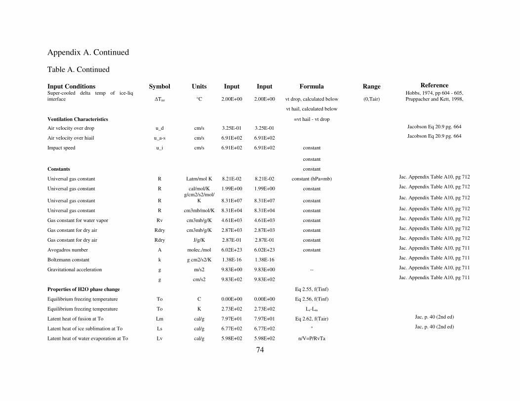
74


Table A. Continued

Input Conditions Symbol Units Input Input Formula Range Reference Super-cooled delta temp of ice-liq interface ∆Tint °C 2.00E+00 2.00E+00 vt drop, calculated below (0,Tair)

Hobbs, 1974, pp 604 - 605, Pruppacher and Kett, 1998,

vt hail, calculated below

Ventilation Characteristics =vt hail - vt drop

Air velocity over drop u_d cm/s 3.25E-01 3.25E-01 Jacobson Eq 20.9 pg. 664

Air velocity over hiail u_a-s cm/s 6.91E+02 6.91E+02 Jacobson Eq 20.9 pg. 664

Impact speed u_i cm/s 6.91E+02 6.91E+02 constant

constant

Constants constant

Universal gas constant R Latm/mol K 8.21E-02 8.21E-02 constant (hPa=mb) Jac. Appendix Table A10, pg 712

Universal gas constant R cal/mol/K 1.99E+00 1.99E+00 constant Jac. Appendix Table A10, pg 712

Universal gas constant R g/cm2/s2/mol/

K 8.31E+07 8.31E+07 constant Jac. Appendix Table A10, pg 712

Universal gas constant R cm3mb/mol/K 8.31E+04 8.31E+04 constant Jac. Appendix Table A10, pg 712

Gas constant for water vapor Rv cm3mb/g/K 4.61E+03 4.61E+03 constant Jac. Appendix Table A10, pg 712

Gas constant for dry air Rdry cm3mb/g/K 2.87E+03 2.87E+03 constant Jac. Appendix Table A10, pg 712

Gas constant for dry air Rdry J/g/K 2.87E-01 2.87E-01 constant Jac. Appendix Table A10, pg 712

Avogadros number A molec./mol 6.02E+23 6.02E+23 constant Jac. Appendix Table A10, pg 711

Boltzmann constant k g cm2/s2/K 1.38E-16 1.38E-16 Jac. Appendix Table A10, pg 711

Gravitational acceleration g m/s2 9.83E+00 9.83E+00 -- Jac. Appendix Table A10, pg 711

g cm/s2 9.83E+02 9.83E+02 Jac. Appendix Table A10, pg 711

Properties of H2O phase change Eq 2.55, f(Tinf)

Equilibrium freezing temperature To C 0.00E+00 0.00E+00 Eq 2.56, f(Tinf)

Equilibrium freezing temperature To K 2.73E+02 2.73E+02 Ls-Lm

Latent heat of fusion at To Lm cal/g 7.97E+01 7.97E+01 Eq 2.62, f(Tair) Jac, p. 40 (2nd ed)

Latent heat of ice sublimation at To Ls cal/g 6.77E+02 6.77E+02 " Jac, p. 40 (2nd ed)

Latent heat of water evaporation at To Lv cal/g 5.98E+02 5.98E+02 n/V=P/RvTa

75


Table A. Continued


Saturation vapor pressure over liquid atair temperature Psat_a mbar 5.28E+00 5.28E+00 n/V = P/RvTw

Jac, p 41

Saturation vapor pressure over liquid at To Psat_w mbar 6.11E+00 6.11E+00 "

"

Saturation vapor density over liquid at Tair rair g/cm3 4.22E-06 4.22E-06 Eq 2.64 /Rv(Tinf+a)

assume atmosphere is saturated w/ respect to water

Saturation vapor density over liquid at To rsat,w g/cm3 4.85E-06 4.85E-06 Eq 14.19, f(Tair)

Ice sat vapor density at Tair rsat,i g/cm3 4.14E-06 4.14E-06 "

Ice sat vapor density at To rsat,i g/cm3 4.85E-06 4.85E-06 Jac, p 43

Water-air surface tension sw/a dyn/cm 7.59E+01 7.59E+01 Eq 4.54, f(Tair) Jac, p 485

Table 4.1, f(Tair)

Properties of dry air Eq 2.5, f(Tair)

Dynamic viscoscity of dry air hdrya g/cm/s 1.71E-04 1.71E-04 Jac, p 102

Heat capacity of dry air at constant pressure Cp,da cal/g/C 2.39E-01 2.39E-01

Smith and Vanness, p 109

Thermal conductivity of dry air ka cal/cm/s/C 5.65E-05 5.65E-05 calculated above Jac, p. 20

εpv/(pa-pv)

Properties of moist air Rdry(1+0.0608qv)

Density of water vapor in air rair g/cm3 air 4.22E-06 4.22E-06 =R/Rm

Mass mixing ratio of water vapor in air wv g/g 4.13E-03 4.13E-03 =Pa/RmT Eq 2.31

Gas constant for moist air Rm cm3mb/g/K 2.88E+03 2.88E+03 Eq 2.37

Molecular weight of moist air Ma g/mol 2.89E+01 2.89E+01 ha/pa Eq 2.26

Density of moist air ra g/cm3 1.03E-03 1.03E-03 Eq 2.36

Dynamic viscoscity of moist air ha g/cm/s 1.71E-04 1.71E-04 calculated above

Kinematic viscoscity of moist air na cm2/s 1.67E-01 1.67E-01 rv/RvTa definition

Mean free path of moist air la cm 7.47E-06 7.47E-06 Eq 8.6

76


Table A. Continued

Input Conditions Symbol Units Input Input Formula Range Reference Heat capacity of moist air at constant pressure Cp,ma cal/g/C 2.40E-01 2.40E-01

Partial pressure of water vapour in air Pair mbar 5.28E+00 5.28E+00 = 0.211(T/To)1.94(Po/P) Eq 2.27

Properties of water vapor

Diffusivity of water vapor in air Dv cm2/s 2.63E-01 2.63E-01 calculated above Eq. 13-3

Properties of liquid water in supercooled drop = (n=0, n=6 ∑anTn

Supercooled drop temperature Tw_s C -2.00E+00 -2.00E+00 =(n=0, n=4 ∑anTn)

Supercooled drop temperature Tw K 2.71E+02 2.71E+02

Density of supercooledwater rw g/cm3 1.00E+00 1.00E+00 Eq 3-14

Heat capacity of water cw cal/g/C 1.01E+00 1.01E+00 calculated above Eq 3-16

calculated above

Properties of hail liquid water (during freezing (at 0C)) = (n=0, n=6 ∑anTn

Water temp. Tw C 0.00E+00 0.00E+00 calculated above

Water temp. Tw K 2.73E+02 2.73E+02

Density of water rw g/cm3 1.00E+00 1.00E+00 P&K p. 87

Saturation vapor density above liquid rsat,w g/cm3 4.85E-06 4.85E-06 calculated above

Properties of ice substrate

temperature of ice substrate Td C -2.00E+00 -2.00E+00

temperature of ice substrate K 2.71E+02 2.71E+02 input paramter

kv (DT)c

Properties of Bulk Hail

Density of Hail (Calculated) ρh g/cm3 9.57E-01 9.57E-01 0.1 (Heymsfield) to 1 g/cm3

Intrinsic ice growth velocity cm/s 1.20E+00 1.20E+00

77


Table A. Continued


Caculation of hail density - problematic, need to explore

Y = -avimp/Ts u m/sC 1.73E+01 1.73E+01

Bulk density of rimed ice g/cm3 1.05E+00 1.05E+00 Heymsfield parameterization P&K, p 661;

Bulk density of rimed ice (for compare only) g/cm3 1.18E+00 1.18E+00 0.11(-B)^0.76

P&K, p 661; Macklin and Payne, 1962( p 41)

Density of pure ice g/cm3 9.17E-01 9.17E-01 Eq 3-2, f(Tice) P&K, p79

Denisty of hail (calculated) g/cm3 9.57E-01 9.57E-01 ((h/rwtr + (1 -h)/rice)^-1 weighted reciprical average

Terminal Fall Velocitiy Calculations For Hail Partice Schmidt Number Sc - 6.32E-01 6.32E-01 υa/Dp eq 16.25

Knudsen Number Kn - 7.47E-05 7.47E-05 λa/ri eq 15.23

Bond Number NBo - 4.95E-01 4.95E-01 eq 20.8

Physical property number NP - 5.75E+11 5.75E+11 eq 20.8

X for polynomial fit X - 1.28E+01 1.28E+01 eq 20.7

Y for polynomial fit Y - 4.10E+00 4.10E+00 "

Cunningham Slip -flow Correction factor G - 1.00E+00 1.00E+00 =1+Kn[A+Bexp(-C/Kn)]

eq 15 .30

Initial Termial Fall Speed (slip flow) Vest cm/s 1.22E+04 1.22E+04 eq 20.4

Initial Reynolds Number (slip Flow) Reest - 1.47E+04 1.47E+04 eq 20.5

Reynolds Numbers Regimes Reynods Number- Slip Flow - 1.47E+04 1.47E+04 eq 20.6

Reynolds Nnmber Continiuum (sphere) - 7.47E+02 7.47E+02 eq 20.6 Reynolds Number Continuum (non-spherical) - 8.30E+02 8.30E+02

eq 20.6

Final Reynolds Number (Hail particle) Refinal - 8.30E+02 8.30E+02 eq 20.6

Final Fall Speed ( Hail particle) Vfinal cm/s 6.91E+02 6.91E+02 eq 29.9

78


Table A. Continued


For Drop Schmidt Number Sc - 6.32E-01 6.32E-01 eq 16.25

Knudsen Number Kn - 1.49E-02 1.49E-02 eq 15.23

Bond Number NBo - 1.29E-05 1.29E-05 eq 20.8

Physical property number NP - 5.51E+11 5.51E+11 eq 20.8

X for polynomial fit X - -3.08E+00 -3.08E+00 eq 20.7

Y for polynomial fit Y - -6.46E+00 -6.46E+00 " Cunningham Slip -flow Correction factor G - 1.02E+00 1.02E+00

eq 15 .30

Initial Termial Fall Speed (slip flow) Vest cm/s 3.25E-01 3.25E-01 eq 20.4

Initial Reynolds Number (slip Flow) Reest - 1.95E-03 1.95E-03 eq 20.5

Reynolds Numbers Regimes Reynods Number- Slip Flow - 1.95E-03 1.95E-03 eq 20.6

Reynolds Nnmber Continiuum (sphere) - 1.86E-03 1.86E-03 eq 20.6 Reynolds Number Continuum (non-spherical) - 2.74E-161 2.74E-161

eq 20.6

Final Reynolds Number (drop) Refinal - 1.95E-03 1.95E-03 eq 20.6

Final Fall Speed (drop) Vfinal cm/s 3.25E-01 3.25E-01 eq 29.9

Turbulent enhancement to heat and water vapor transfer from hail

Gas Phase

Prandtl number (molecular mom./heat transfer) Pr 7.25E-01 7.25E-01 ηaCp/ka

Eq 16.32

Schmidt number (water vapor) Scv 6.32E-01 6.32E-01 υa/Dv Eq 16.25

Stokes Number w/o Cd Ns 2.25E+00 2.25E+00 rwUDd2 / 9maDs Eq 4-11

24/CDRe for drop 1.00E+00 1.00E+00 Eq 8.32

79


Table A. Continued


Stokes Number w Cd Ns 2.25E+00 2.25E+00 =Ns 24/CDRe after P&K, p 573 and S&P, p.

487,465

Nusselt No - smooth cylinder (Avila) Nu_o 1.30E+01 1.30E+01 c RemPrn Incopera and Dewitt, 1996,

p.345, Eqn 7.47

Nusselt No - smooth cylinder(Incopera) 1.47E+01 1.47E+01 for smooth cylinder Incopera and Dewitt, 1996,

p.345, Eqn 7.47

Nusselt No (heat) - riming cylinder Nu 2.55E+01 2.55E+01 Eqn 9

Sherwood No (water vapor) - smooth Sh_o_v 1.24E+01 1.24E+01 like Nu Eqn 5

Sherwood No (water vapor)- riming Sh_v 2.43E+01 2.43E+01 Eqn 9

Ventilation coeff (water vapor) f - 1.21E+01 1.21E+01 Sh/2

Determination of Schumann-Ludlam limit for wet vs dry growth Efficiency of collection E 1.00E+00 1.00E+00 same as Lin et al., 1

Shape factor in equation F 4.00E+00 4.00E+00 For clyindr = pi ; For a sphere =

4

Critical liquid water content W_c g/cm3 2.09E-06 2.09E-06 heat balance, Ts=0

Critical liquid water content W_c g/m3 2.09E+00 2.09E+00

Growth regime Wet Wet =πr2vω* eff collection =4πrDF(Psat/RTh - Pa/RTa)

Water mass rates Mass rate of drop accretion F g/s 6.51E-05 6.51E-05 Mass Rate of water Evaporation E g/s 2.53E-06 2.53E-06 Intrinsic ice growth g/s 1.44E-01 1.44E-01 =4πr2Kv(∆tint)crice Allowable ice growth g/s 3.13E-05 3.13E-05 =η/(1-η)*Gm

Mass rate of ice crystal growth Gm g/s 3.13E-05 3.13E-05 =Gm + Lw Eq 6.17 (Stuart 2000, PhD

Dissertation, p135)

Mass rate of change of liquid water in hail Lw g/s 3.13E-05 3.13E-05

assumes constant liquid water content in hail

Mass Growth rate G g/s 6.26E-05 6.26E-05 derived from initial model

equation.

Mass Growth check 6.26E-05 6.26E-05

Mass Rate of Drop Shedding S g/s 0.00E+00 0.00E+00 F-E-G assumes constant liquid water

content in hail

80


Table A. Continued


Calculation of Retention keff 1.00E-03 1.00E-03 1-keff 9.99E-01 9.99E-01 h 5.00E-01 5.00E-01 1-h 5.00E-01 5.00E-01 1/H* Cair/Cwtr 9.69E-14 5.86E-10 rL g/cm3 1.00E+00 1.00E+00 rVLsat g/cm3 4.85E-06 4.85E-06 rL / rlVsat 2.06E+05 2.06E+05 n G/F 9.61E-01 9.61E-01 m E/F 3.88E-02 3.88E-02

numerator h + keff (1-h) 5.01E-01 5.01E-01

denominator 1-n-m (shedding effect) -1.04E-16 -1.04E-16 n(h+keff(1-h)) (growth effect) 4.81E-01 4.81E-01 m(1/H*rL / rvl) (evaporation effect) 7.75E-10 4.69E-06

total denominator 4.81E-01 4.81E-01

Retention ratio Г - 1.04E+00 1.04E+00 =h+ke(1-h) / 1-[1-h-ke(1-)]n-[(1-1/H*(rL / rvlsat)]m

Mass Balance Testing Water Mass Balance Check g/s 0.00E+00 0.00E+00 Should be zero

Solute mass balance Average mixing ratio of chemical in air pptv 5.00E+01 5.00E+01 Seinfeld & Pandis, pg 61

Ca g/cm3 1.12E-13 3.02E-14 =pptv/1e12*P/RT*MW

81


Table A. Continued


solute mass fraction_drop Xd g_chem/g_wtr 1.15E+00 5.15E-05 =Ca*H/rwtr

solute mass fraction_hail Xh g_chem/g_wtr 1.20E+00 5.36E-05 =GXd

solute mass fraction_shed liquid Xl g_chem/g_wtr 2.40E+00 1.07E-04 =Xh/(h+keff(1-h) solute mass fraction_evap sol'n Xe g_chem/g_wtr 4.79E-08 1.29E-08 =Xl*(1/H)*(rl/rvlsat)

solute mass in via accretion Xd*F g_chem/s 7.52E-05 3.35E-09

solute mass out via shedding Xl*S g_chem/s 0.00E+00 0.00E+00

solute mass out via evaporation Xe*E g_chem/s 1.21E-13 3.27E-14

solute mass accumulation in hail Xh*G g_chem/s 7.52E-05 3.35E-09

solute mass balance check check g_chem/s 0.00E+00 0.00E+00 should be zero

retention check 1.04E+00 1.04E+00

About the Author

Ryan Algernon Michael was born in New Amsterdam, Guyana. He completed his

undergraduate degree at the University of Guyana during the fall of 2005, majoring in

chemistry, with biology minor. He graduated with honors, and as awarded the Dean’s

Award for the Best Graduating Chemistry Student, as well as the University of Guyana

Award for the Best Graduating Natural Science Student. He worked briefly at Berger

Paints, Barbados Ltd, in the Quality Control Department for paint production. Ryan

received a Master of Engineering Sciences degree from the University of South Florida in

the fall of 2008.

Documents

Fate of Volatile Chemicals during Accretion on Wet-Growing