Embed Size (px)
Citation preview

Fatigue Analysis ofOverhead Sign andSignal StructuresPhysical Research Report No. 115
L-
Time (see)
Illinois Department of TransportationBureau of Materials and Physical Research

TECNNICAL REPORT STANDARD TITLE PAGE
1. R-pwt No. 2. Govornmsnt ACCOSIIOIIh. 3. Rocipktt’ s Cotoba No.
FHWA/IL/PR-l 15
4. Titlo and Subtitlo 5. Rspert Data
FATIGUE ANALYSIS OF OVERHEAD SIGN ANDMay 1994
SIGNAL STRUCTURESb. Porfom#n90rgent xot, on Cod*
7. Adds) ,8. Performing OrSmtxatton Report No,
Jeffrey M. South, P.E. PRR-115
9. Po.fermtnq Org~#zataon N~o md Addros8 10. Werk Unit No.
Illinois Department of TransportationBureau of Materials and Physical Research 11.Contract or Grant No.
126 East Ash Street IHR-319
Springfield, Illinois 62704-4706 13.Typo of Raport and P=riod Covwod7
iz. spomsertng Aqoncy Nmno ond Addros- Interim Report:
Illinois Department of Transportation July 1990 through
Bureau of Materials and Physical Research May 1994
126 East Ash Street 14. s~”se,,”g Agency Coda
Springfield, Illinois 62704-4706IS.supP/omontory NO**S
Study conducted in cooperation with the U.S. Department of Transportation,Federal Highway Administration.
16. Abat,ocf This report documents methods of fatigue analysis for overhead sign and signal structures. The
main purpose of this report is to combine pertinent wind loading and vibration theory, fatigue damage
theory, and experimental data into a useable fatigue analysis method for overhead sign and signal
structures. Vibrations and forces induced by vortex shedding were studied analytically and measured
experimentally. Analytical models were extracted from the literature. Drag coefficients, generally assume
to be constants or simple functions of Reynolds number, actually depend on the amplitude of vortex shedding
vibration. The amplification of drag coefficients can have a significant effect on resulting forces.
Fatigue and the concept of fatigue damage quantification were discussed. Fatigue was described as a failut-
mode which results from cyclic application of stresses which may be much lower than the yield stress.
Fatigue damage was quantified using the Palmgren-Miner linear damage equation. Available stress cycles For
each applied stress range are calculated by expressing published S-N fatigue data for welds or anchor bolts
as N–S equations, where number of available cycles (N) is the dependent variable, instead of stress range.
The use and limitations of fracture mechanics methods were discussed. Stress concentrations were discussed
as a vital parameter in fatigue analysis. Methods for estimating Kt for fillet welds and anchor bolt
threads were extracted from the literature. Experimental data were collected for a representative traffic
signal structure. This data included stress range and frequency response for ambient wind loadings, dead
load stresses, strain as a function of vertical tip deflection, vibration frequency due to ambient winds,
and strain response due to controlled-speed wind loads. The instrumented details were tube to base plate
circumferential fillet welds and anchor bolts. Wind speed data were collected at a traffic signal site in
Springfield, Illinois for seventeen months. Factor of safety equations for use with welded details were
discussed. Sample fatigue life calculations using both strain gage-derived and analytically estimated
stress range-frequency histograms were performed as examples to the reader. Calculations using static
conditions were also performed. The results differed siqnificantlv from t.h~ other <ol!,Linn~
17. Koy Words 18. DiS*lktiOtl!ita?omsntFatigue, wind forces, safety factors, No restrictions. This document is avail-strain gages, histogram-linear damage able to the public through the Nationalrule. Technical Information Service, Springfield,
Virginia 22161.
19. Swurlty Ciasslf.(oftillsr-port) 20.Securtty Cla~wi. (ef this pogo) 21. No. of poges 22.Prtco
Unclassified Unclassified 118
Form DOT F 1700.7 (8-69]

FATIGUE ANALYSISOF
OVERHEAD SIGNAND
SIGNAL STRUCTURES
Jeffrey M. South, P. E.Engineer of Technical Services
Physical Research Report Number 115Illinois Department of Transportation
Bureau of Materials and Physical Research
May 1994

FORE140RD
This report shou
design, planning, ma
d be of interest to engineers involved in structural
ntenance and inspection; consultants, and other technical
personnel concerned with the fatigue life of structures.
NOTICE
The contents of this report reflect the views of the author who is
responsible for the facts and the accuracy of the data presented herein.
The contents do not necessarily reflect the official views or policy of the
Federal Highway Administration or the Illinois Department of Transportation.
This report does not constitute a standard, specification, or regulation.
Neither the United States Government nor the State of Illinois endorses
products or manufacturers. Trade or manufacturers’ names appear herein solely
because they are considered essential to the object of this report.

ACKNO14LEDGMENTS
The author gratefully acknowledges the kind assistance and
support of:
Mr. Christopher Hahin, Engineer of Bridge Investigations;
Ms. Mary Milcic, Research Engineer; Mssrs. Dave Bernardin,
Tom Courtney, Russ Gotschall, Harry Smith, Ken Wyatt, and
Brian Zimmerman. The typing efforts of Ms. Bev Buhrmester
are gratefully acknowledged.

TABLE OF CONTENTS
Paue
List of Figures
List of Tables
1.
‘ 2.
3.
4.
5.
6.
7.
8.
9.
Introduction
Wind-Induced Forces and Vibrations
Hind Speed Data
Strain Gage and Frequency Data
Determination of Fatigue Damage to Components
Sample Fatigue Damage Analyses Using BothStrain Gage Methods and Analytical Methods
Factor of Safety Equations for Fatigue Design
Summary
Conclusions and Recommendations
i
v
1
4
19
35
76
88
99
102
105
References 107

LIST OF FIGURES
Fiqure No.
1
2
3
4
5
6
8
9
10
11
Descri~tion
Representation of the vortex sheddingprocess. U is the windspeed, D iscylinder diameter, Ay is transversedeflection due to vortex shedding.
A flow chart for estimating amplitudeand drag for vortex-induced vibration.
A flow chart for estimating lift forcesfor vortex-induced vibrati&.
Wind speed versus frequency ofhistogram for signal structureat White Oaks Drive in Springffor calendar year 1992.
occurrenceat Illinois 54eld, Illinos
Wind speed data collected at Illinois 54 atWhite Oaks Drive in Springfield, Illinoison January 8, 1992. Data were collected atone–minute intervals.
Nind speed data collected at Illinois 54 at“White Oaks Drive in Springfield, Illinoison February 26, 1992. Data were collected atone-minute intervals.
7 Wind speed data collected at Illinois 54 atWhite Oaks Drive in Springfield, Illinoison March 3, 1992. Data were collected atone-minute intervals.
Hind speed data collected at Illinois 54 atWhite Oaks Drive in Springfield, Illinoison April 29, 1992. Data were collected atone-minute intervals.
Wind speed data collected at Illinois 54 atWhite Oaks Drive in Springfield, Illinoison May 16, 1992. Data were collected atone-minute intervals.
Wind speed data collected at Illinois 54 atWhite Oaks Drive in Springfield, Illinoison June 2, 1992. Data were collected atone-minute intervals.
blind speed data collected at Illinois 54 atWhite Oaks Drive in Springfield, Illinoison July 27, 1992. Data were collected atone-minute intervals.
~
6
17
18
22
23
24
25
26
27
28
29
i

LIST OF FIGURES (CONTINUED)
Fiqure No.
12
14
15
16
17
18
19
20
21
Descrl~tion
Wind speed data collected at Illinois 54 atWhite Oaks Drive in Springfield, Illinoison August 18, 1992. Data were collected atone–minute intervals.
Wind speed data collected at Illinois 54 at14hiteOaks Drive in Springfield, Illinoison September 1, 1992. Data were collected atone-minute intervals.
blind speed data collected at Illinois 54 atWhite Oaks Drive in Springfield, Illinoison October 30, 1992. Data were collected atone–minute intervals.
Wind speed data collected at Illinois 54 atWhite Oaks Drive in Springfield, Illinoison November 7. 1992. Data were collected atone–minute intervals.
Wind speed data collected at Illinois 54 aWhite Oaks Drive in Springfield, Illinoison December 22, 1992. Data were collectedone-minute intervals.
Instrumented traffic signal mastarm instal’
at
edat Physical Research Laboratory in Springfield,Illinois. Strain gage locations are shown.
Instrumented section of traffic signal structurefor controlled wind speed tests. Testing andinstrumentation were conducted at Smith-EmeryCompany, Los Angeles, California. Strain gageswere placed at 12, 3, 6, and 9 o’clock positionsnear the toe of the fillet weld.
Data acquisition system used for controlledwind speed tests.
Equipment and setup used to apply wind loads.Technician is checking wind speed with ahand-held anemometer.
Eighty mile per hour wind load being applied totraffic signal structure.
ii
!b41e
30
31
32
33
34
36
45
46
47
48

LIST OF FIGURES (CONTINUED)
Fiaure No.
22
23
24
25
26
27
28
29
30
31
32
33
34
35
Lift stresses20 mph contro
Lift stresses40 mph contro
Lift stresses
Description
at top strain gage due toled wind application.
at top strain gage due toled wind application.
at top strain gage dueto 50 mph controlled wind application.
Lift stresses at top strain gage due to60 mph controlled wind application.
Lift stresses at top strain gage due’to70 mph controlled wind application.
Lift stresses80 mph contro’
Drag stresses(facing wind)wind applicat
Drag stresses(facing wind)
at top strain gage due toled wind application.
at west strain gagedue to 20 mph controlledon.
at west strain gagedue to 40 mph controlled
wind application.
Drag stresses at west strain gage(facing wind) due to 50 mph controlledwind application.
Drag stresses at west strain gage(facing wind) due to 60 mph controlledwind application.
Drag stresses at west strain gage(facing wind) due to 70 mph controlledwind application.
Drag stresses at west strain gage(facing wind) due to 80 mph, controlledwind application.
Lift stresses at bottom strain gage due to20 mph controlled wind application.
Lift stresses at bottom strain gage due to40 mph controlled wind application.
iii
!39-!2
50
51
52
53
54
55
56
57
58
59
60
61
62
63
Fiuure No.
36
37
38
39
40
41
42
43
44
45
46
47
LIST OF FIGURES (CONTINUED)
Description
Lift stresses at bottom strain gage due to50 mph controlled wind application.
Lift stresses at bottom strain gage due to60 mph controlled wind application.
Lift stresses at bottom strain gage due to70 mph controlled wind application.
Lift stresses80 mph contro
Drag stresses20 mph contro
Drag stresses
at bottom strain gage due toled wind application.
at east strain gage due toled wind application.
at east strain gage due to40 mph controlled wind application.
Drag stresses at east strain gage due to50 mph controlled wind application.
Drag stresses at east strain gage due to60 mph controlled wind application.
Drag stresses at east strain gage due to70 mph controlled wind application.
Drag stresses at east strain gage due to80 mph controlled wind application.
Stress concentration factor, Kt, for astepped, round bar with a shoulder filletin bending, from Peterson. Used withpermission.
Stress concentration factor, Kt, for agrooved shaft in tension, from Peterson.Used with permission.
~
64
65
66
67
68
69
70
71
72
73
86
87
iv

Table No.
1
2
3
4a
4b
5
6
7
8
9
10
11
12
13
14
15
LIST OF TABLES
Descri~tion
Reynolds Number Regimes for VortexShedding from Smooth Circular Cylinders.
Dimensionless Mode Factors for SomeStructural Elements and Natural Frequencies.
Measured Wind Speeds and Frequency ofOccurrence.
Stress Range-Frequency Data for InstrumentedFillet Weld Connection on Traffic SignalMastarm.
Stress Range-Frequency Data for InstrumentedAnchor Bolts for Cantilevered Traffic SignalStructure.
Measured Dead Load Strains on Traffic SignalStructure.,
Measured Strain Versus Tip Deflection.
Statistics for Controlled Hind Speed TestData.
Apparent Drag Coefficient for In-Place TrafficSignal Using Average Strain Data.
FatforAWS
Fatfor
gue Strength Coefficients and ExponentsVarious Welded Tubular Steel Details,Data.
gue Strength Coefficients and ExponentsSome Steels.
Expected Fatigue Damage Calculation forTraffic Signal Mastarm Using Strain Gage Data.
Parameters Used for Analytical Fatigue LifeEstimation.
Wind Speeds at Which Synchronization isExpected.
Calculated Drag Stresses on Mastarm for EachMeasured Wind Speed.
Expected Fatigue Damage Estimation UsingMeasured Wind Speed Data.
v
!?.a9E
7
13
21
37
38
39
41
49
74
79’
82
88
92
92
94
95

1
1. INTRODUCTION
The unexpected failure of an overhead sign or signal structure could
result in serious injuries, property damage, and/or increased traffic
congestion and accidents.
Overhead structures intended to support signs or traffic signals are
designed to resist dead loads, live loads, ice loads, and wind loads.’
Dead loads include the weight of the member, signs, traffic signals, or
other attachments. Live loads are defined as walkways and service
platforms. Ice loads are used in areas of the country where winter ice
buildup is expected. The wind load is idealized as a maximum pressure
based on mean recurrence intervals of a maximum wind speed for the
location of service, member shape, and height above ground of the member
being loaded. All loads are considered to be static for design purposes.
However, overhead sign and signal structures are subjected to varying
wind loads every day. In addition, vortex shedding induces cyclic loads.
The variability of these forces from day to day and even from instant to
instant implies that these structures are sustaining some amount of
cumulative fatigue damage. The cyclic nature of the actual stresses
experienced, and therefore, the potential for fatigue damage and failure
is not accounted for in the design process. A need exists for rational
methods to evaluate the expected fatigue life of overhead sign and signal
structures and for methods to assess the fatigue susceptibility of new
structures while in the design phase.
The number of overhead sign and signal structures in service is
surprising. These structures occur at nearly every modern urban inter-
section with three or more lanes. Large overhead sign structures are2
found both before and at nearly every interchange on the interstate system

2
and on other divided highways. The large number of these structures and
the cost to build or replace them requires some study of their fatigue
behavior.
There are many types of overhead structures in service. Traffic
signs’
signs’
frame
structures in particular show wide variety. Popular cantilevered
structures include straight and arced tapered single arm and plane
mastarms. Tubular cross-sections in use include circular, hexdec-
agonal (16-sided), dodecagonal (lZ-sided), octagonal, square, and
elliptical. Materials used include steel and aluminum. Sign structures
include cantilevered space frames with rectangular gross cross-sections
and simply supported space frames with both rectangular and triangular
cross-sections. The most common components used in overhead sign structure
applications are circular tubes, although plane frame structures with
rectangular tube or I–shaped cross-sections are becoming popular for new
construction.
Fatigue is a failure mode that involves repeated loading at stress
levels which may be only a small fraction of the tensile strength of a
particular material. Because fatigue failures result from repeated
loadings, it is characterized as a progressive failure mode that proceeds
by the initiation and propagation of cracks to an unstable size. Each
stress cycle ~auses a certain amount of damage. Depending on applied
stress levels and material properties, component fatigue lives can range
from a few hundred to more than 108 cycles to failure. The most common
sites of fatigue failures in components are at areas of stress
concentrations. Welds, notches, holes, and material impurities such as
I

3
slag inclusions are examples of stress concentrations. Not surprisingly,
common fatigue cracking areas in overhead sign and signal structures are
at welds and anchor bolts (threads are sharp notches).
The fatigue life of a component may be thought of in two phases.
Crack initiation life is that portion of fatigue life which occurs before
a crack forms. Crack propagation life is the portion of fatigue life
which occurs between crack formation and unstable crack growth.
Typically, for the steels used in sign and signal structures, the
initiation life for a weld detail is far longer than the propagation
life. This implies that once a crack appears, especially in a
nonredundant structure, the fatigue life of that detail is effectively
used up, and the component could rupture relatively quickly.
The purposes of this report are to combine pertinent existing wind
loading and vibration theory, fatigue damage theory, and experimental data
into a usable fatigue analysis method for overhead sign and signal
structures and to outline factor of safety equations for estimation of
weld detail fatigue susceptibility.
4
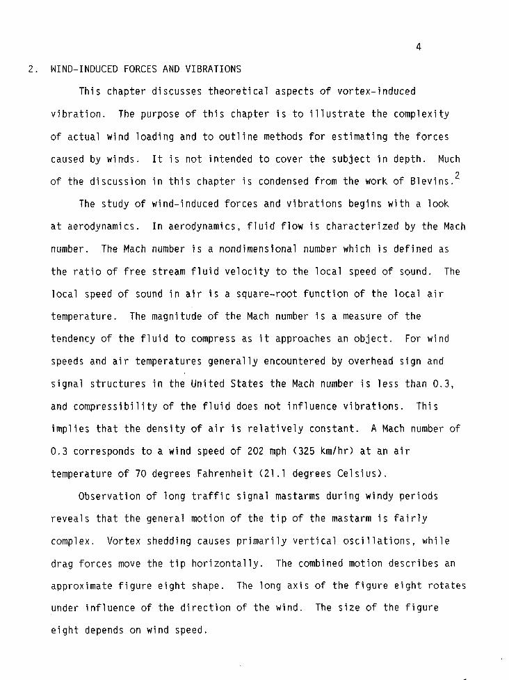
2. WIND-INDUCED FORCES AND VIBRATIONS
This chapter discusses theoretical aspects of vortex-induced
vibration. The purpose of this chapter is to illustrate the complexity
of actual wind loading and to outline methods for estimating the forces
caused by winds. It is not intended to cover the subject in depth. Much
of the discussion in this chapter is condensed from the work of Blevins. 2
The study of wind-induced forces and vibrations begins with a look
at aerodynamics. In aerodynamics, fluid flow is characterized by the Mach
number. The Mach number is a nondimensional number which is defined as
the ratio of free stream fluid velocity to the local speed of sound. The
local speed of sound in air is a square-root function of the local air
temperature. The magnitude of the Mach number is a measure of the
tendency of the fluid to compress as it approaches an object. For wind
speeds and air temperatures generally encountered by overhead sign and
signal structures in the United States the Mach number is less than 0.3,
and compressibility of the fluid does not influence vibrations. This
implies that the density of air is relatively constant. A Mach number of
0.3 corresponds to a wind speed of 202 mph (325 km/hr) at an air
temperature of 70 degrees Fahrenheit (21.1 degrees Celsius).
Observation of long traffic signal mastarms during windy periods
reveals that the general motion of the tip of the mastarm is fairly
complex. Vortex shedding causes primarily vertical oscillations, while
drag forces move the tip horizontally. The combined motion describes an
approximate figure eight shape. The long axis of the figure eight rotates
under influence of the direction of the wind. The size of the figure
eight depends on wind speed.

5
Vortex Shedding
Vortex shedding
structures. Vortices
s a phenomenon which occurs in subsonic flow past
are shed from one side of a member and then the
other. As this continues, oscillating surface pressures are imposed on
the structure. The oscillating pressures cause elastic structures to
vibrate. A description of the process of vortex shedding is given by
Blevins.3
“AS a fluid particle flows toward the leading edge of acylinder, the pressure in the fluid particle rises from thefree stream pressure to the stagnation pressure. The highfluid pressure near the leading edge impels flow about thecylinder as boundary layers develop about boths ides.However, the high pressure is not sufficient to force theflow about the back of the cylinder at high Reynoldsnumbers. Near the widest section of the cylinder, theboundary layers separate from each side of the cylindersurface and form two shear layers that trail aft in theflow and bound the wake. Since the innermost portion ofthe shear layers, which is in contact with the cylinder,moves much more slowly than the outermost portion, theshear layers roll into the near wake, where they foldon each other and coalesce into discrete swirlingvortices. A regular pattern of vortices, called a vortexstreet, trails aft in the wake. The vortices interact withthe cylinder and they are the source of the effects calledvortex–induced vibration.”
A representation of the vortex shedding process is shown in Figure 1.
Vortex shedding from smooth, circular cylinders with steady subsonic flow
is a function of the Reynolds number. The Reynolds number is given by:
Re=l+ (1)
where U = free stream velocity,D = cylinder diameter,v = kinematic viscosity of the fluid,
. 1.564 x 10⁻⁴ ft2/sec (1.681 x 10⁻³m2/see) for air.
The Reynolds number is the ratio of the inertia force and the
friction force on a body. The Reynolds number is a parameter used to
indicate dynamic similarity. Two flows are dynamically similar when the
Reynolds number is equal for both flows.

6
F.1gure 1. Representa
the
def
t ion of
windspeed
ection due
D
the Vor
is CyIi
tex sheed ng
riderdiameter
to vortex shedding.
9
proce s
AY
s
is
a
u is
transverse
7
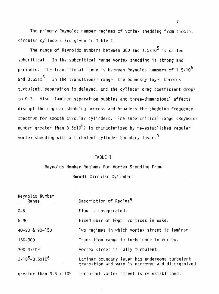
The primary Reynolds number regimes of vortex shedding from smooth,
circular cylinders are given in Table I.
The range of Reynolds numbers between 300 and 1.5x10⁵ is called
subcritical. In the subcritical range vortex shedding is strong and
periodic. The transitional range is between Reynolds numbers of 1.5x10⁵
and 3.5x10⁶. In the transitional range, the boundary layer becomes
turbulent, separation is delayed, and the cylinder drag coefficient drops
to 0.3. Also, laminar separation bubbles and three-dimensional affects
disrupt the regular shedding process and broadens the shedding frequency
spectrum for smooth circular cylinders. The supercritical range (Reynolds
number greater than 3.5x10⁶) is characterized by re-established regular
4vortex shedding with a turbulent cylinder boundary layer.
TABLE I
Reynolds Number Regimes For Vortex Shedding From
Smooth Circular Cylinders
Reynolds NumberRanqe
o-5
5-40
40-90 & 90-150
150-300
3OO-3X1O5
3X10⁵-3.5X1O6
greater than 3.5 x 10⁶
Description of Reuime5
Flow is unseparated.
Fixed pair of Foppl vortices in wake.
Two regimes in which vortex street is laminar.
Transition range to turbulence in vortex.
Vortex street is fully turbulent.
Laminar boundary layer has undergone turbulenttransition and wake is narrower and disorganized.
Turbulent vortex street is re-establ ished.
8
The Strouhal number is the dimensionless proportionality constant
which relates the predominant vortex shedding frequency, the free stream
velocity, and the cylinder width. It is given by:
S = fsD/U (2)
where fs = vortex shedding frequency, Hertz (cycles/second),u = free stream velocity,D = cylinder diameter.
Vortex-induced vibration of cylinders generally occurs at S-0.2 in
the transitional Reynolds number regime. An interesting experimental
result is that lift oscillations occur at the vortex shedding frequency,
while drag oscillations occur at twice the vortex shedding frequency due
to the geometry of the vortex street.
Previous discussions were centered on circular cross sections.
However, noncircular sections also shed vortices. The vortex street wake
is formed by the interaction of two free shear layers that trail behind a
structure. Roshko,6’7 Griffin,8 and Sarpkayag suggest that it is
possible to define a “universal” Strouhal number for any section based on
the separation distance between the free shear layers. Therefore, if the
characteristic distance D in the Strouhal equation (2) is defined as the
distance between separation points, then the Strouhal number is approxi-
mately 0.2 ove’r wide ranges of Reynolds number regardless of the section
geometry.10
Vortex shedding causes transverse (perpendicular to free stream flow)
vibration of the affected body. Increased amplitude of transverse
cylinder vibration (Ay) can increase the ability of the vibrat
lock-in, ,or synchronize, the shedding frequency. The range of
over which cylinder vibration controls the shedding frequency
on to
frequencies
s known as

9
the lock-in band. Large amplitude cylinder vibration (Ay/D from 0.3 to
0.5) can shift the vortex shedding frequency by as much as t 4(XLfrom the
stationary cylinder shedding frequency. 11
The steady drag force per unit length on a cylinder is given by:
FD = (1/2)@J2DCD (3)
where p = fluid density,0.002378 slug/ft3 (9.85 x 10⁻⁴ kg/m3) for air,
U ~ free stream velocity,D = cylinder diameter,CD = drag coefficient.
The amplitude of cylinder vibration affects the drag coefficient.
Increasing amplitude (Ay) causes the drag coefficient to increase,
sometimes substantially. One expression for relating the increase in drag
coefficient to vibration amplitude is:
C’D=CD [1 + 2.1(AY/D)] (4)
where C’D = Amplitude-influenced drag coefficient,CD = steady flow drag coefficient,Ay = cylinder vibration amplitude,D= cylinder diameter.
Other, more involved equations are also given by Blevins, but the
expressions are within 15% of each other at resonance, and (4) is the
easiest to use directly. The synchronization effect also occurs with
square, triangular, D sections, and other sections that have sharp
separation points. Blevins states that probably all noncircular sections,
in addition to circular sections, that shed vortices will synchronize and
increase drag with resonant transverse vibration. 12 Large amplitude
vibrations can result from synchronization of the vortex shedding
frequency with the structure frequency. In other words, when the flow

10
velocity reaches a value such that the shedding frequency approaches the
natural frequency (or a harmonic or subharmonic) of a structure, the
structure will resonate. This occurs when:
fn - fs = SU/D, or U/fnD_U/fsD = 1/S (5)
where fs = vortex shedding frequency,fn = natural frequency,U = free stream velocity,D = diameter,S = Strouhal number.
Therefore, a combination of U/fD-5 can cause synchronization in a
structure for an assumed fixed Strouhal number of 0.2.13
Analytical Models for Vortex Sheddinu Response
The purpose of this section is to overview and discuss two analyt
models for vortex induced vibration of circular cylindrical structures
The first case is a simple linear harmonic model; the second case is a
nonlinear, self-excited oscillator model.
cal
Since vortex shedding is observed to be an approximately sinusoidal
process (recall the figure eight discussion), a simple way to model the
transverse vortex shedding force is as a harmonic in time at the
shedding frequency. This lifting force is given by:
FL(t) = (1/2)pu2DcLsin(w@ (6)
where FL = lift force (transverse to mean flow) per unit lengthof cylinder,
p = fluid density,U = free stream velocity,D = cylinder diameter,CL = lift coefficient, dimensionlessws = 2xfs = circular vortex shedding frequency,
radians/see, where fs is given by (2),t = time, sec.

11
The lift force is applied as a forcing function to the equation of
motion for an elastically supported, damped, rigid cylinder which may only
move perpendicularly to the flow. The steady-state solution for the
deflection y(t) is assumed to be a sinusoidal response in which A isY
the amplitude of vibration. Substitution back into the equation of motion
gives an expression for y/D. The response reaches a maximum at resonance,
and the resulting resonant amplitude is:
AYJD = CLJ4~S2~r
Where CL = lift coefficient,S = Strouhal number,~r = reduced damping.
The reduced damping term, ~r, is defined as the mass ratio times .
(7)
the structural damping factor
br = 2m(2z~)/flD2
i4here m = mass per unit~ = damping factor
and is given by:
ength including added mass,
(8)
P= density of surrounding fluid,D = diameter of cylinder.
The mass ratio, m/(3D 2, mentioned above, is a measure of the
relative importance of bouyancy and added mass effects on the model. It
is used to mea,sure the susceptibility of lightweight structures to
flow-induced vibration. The likelihood of flow-induced vibration
increases with increasing mass ratio. The damping factor, ~ ,
characterizes the energy dissipated by a vibrating structure. The damping
factor is expressed as a fraction of 1, which is the critical damping
factor. For linear, viscously damped structures, 2x1, is the natural
logarith~ of the ratio of the amplitudes of any two successive cycles of
12
a lightly damped structure in free decay. Many real structures are
lightly damped and so have damping factors on the order of 0.01. The
amplitude of flow-induced vibration usually decreases with increasing
reduced damping.
Note that the right-hand side of (7) implies that the peak amplitude
is independent of flow velocity. This occurs because fixing the Strouhal
number fixes the relationship between cylinder and fluid frequencies.
Blevins14 mentions that actual cylinder response is limited because
the resonant cylinder motion feeds back into the vortex shedding process
to influence the lift coefficient. That is, CL is a function of Ay
for resonating cylinders. The Blevins and Burton model is a three term
polynomial curve fit to experimental data which relates CL to Ay/D:
This
cylinders
CLe = ().35+ 0.60(Ay/D) - o.93(Ay/D)2 (9)
model was developed for vortex-induced vibration of circular
in the subcritical Reynolds number range (Re=300 to
, ~x,05) 15. One drawback for using the harmonic model is that the
calculation of Ay/D in (7) requires a prior estimate of the lift
coefficient CL.
The second analytical model is a nonlinear oscillator with
self-excitation properties. This is known as the wake oscillator model.
The basic
1)
2)
3)
assumptions are:
Inviscid flow provides a good approximation for the flow fieldoutside the near wake.
A well-formed, two-dimensional vortex street with a well-definedshedding frequency exists.
The force exerted on the cylinder by the flow depends on thevelocity and acceleration of the flow relative to the cylinder.
The characteristics of this model are such that cylinder
fed back into the response at synchronization.
by the nonlinear term. The maximum resonant d
predicted in terms of reduced damping (~r) and
13
motion is
This response is limited
sp”acement amp’ itude is
is given by:
Ay/D =
2[ I
1/20.07Y 0.3 + 0.72
(1.9 +br)S (1.9+br)S(lo)
where i%- = reduced damping (see Eq 8),S = Strouhal Number, andv = dimensionless mode factor (see Table 2).
Table 2 gives examples of the mode factor for some structural
elements and natural frequencies.
TABLE 2
Dimensionless Mode Factors (V) ForSome Structural Elements and Natural Frequencies16
StructuralElement
Rigid Cylinder
Uniform PivotedRod
Taut Stringor Cable
Simply SupportedUniform Beam
Cantilevered UniformBeam
NaturalFreauency*
lmi
w, = 3.52-
W2 = 22.03v~”
W3 = 61.70ti~
Y
1.000
1.291
1.155 for n= 1,2,3...
1.155 for n= 1,2,3...
V1 = 1.305
V2 = 1.499
V3= 1.537
‘Where m = mass/unit length,E = modulus of elasticity,I = area moment of inertia of section,L = spanwise length,K = linear spring constant,Ke = torsional spring constant,T = tension force in cable.

14
Calculation of Lift and Dra~ Forces
Note that the lift and drag forces, FL and FD, respectively, are
functions of the lift and drag coefficients, CL and CD, which were
shown to be functions of the vertical deflection amplitude, A TheY“
drag forces increase with increasing Ay, while lift forces increase to a
maximum value, then decrease with increasing A .Y
Ay/D for increasing CLe is estimated to be 0.323.
calculated by differentiating (9) with respect to
equal to zero. The corresponding value of CLe is
The maximum value of
This estimate was
Ay/D and setting it
0.447. This behavior
is in contrast to the method currently used for calculation of wind forces
for design of overhead sign and signal structures, in which CD is a
function of wind velocity and diameter (Reynolds Number) for cylindrical,
hexdecogonal, dodecagonal, and elliptical shapes, and a constant for other
17shapes. Lift forces are not considered in current design procedures.
The question of whether the amplitudes are significant or not is
important. Obviously, if the amplitude of vibration is less than a
certain level, force calculations become simplified because CL and CD
are easier to identify. Blevins defines the amplitude criteria as a
function of both reduced damping and frequency ratio. Ifdr is less
than 64 and fn/fs is between 0.6 and 1.4, then significant amplitudes
18will result.
The calculation procedures for FL and FD resulting from the
previous discussions are complex and require calculation of several
nondimensional parameters as well as estimates of natural frequencies and
structural damping.

15
Figure 2 provides a flow-chart for estimating amplitude and drag in
vortex-induced vibration. Figure 3 shows an additional flow-chart for
estimating lift. Tapered tubes may be treated by dividing the tube into
several stepped uniform members of reasonable length for force calcula-
tions or by using a uniform tube of equivalent stiffness. Thus, both lift
and drag forces induced by vortex shedding may be calculated given the
various input parameters. Stresses at welds or other points in the
structure are then calculated by conventional methods, taking applicable
stress concentration effects into account.
The American Association of State Highway and Transportation
Officials (AASHTO) publishes “Standard Specifications for Structural
Supports for Highway Signs, Luminaires, and Traffic Signals,” which
presents a formula for calculating the wind pressure on a structure: 19
P = 0.00256(1 .3V)2 CDCh (11)
14here P = wind pressure, lbs/ft2,V = wind velocity, mph,CD = drag coefficient, andCh = height coefficient.
This formula is similar to (3) with a thirty percent gust factor and a
coefficient to account for height above ground. One difference between
(3) and (11) is in the intended use. Equation (11) is intended for
calculating static pressures using an isotach chart to predict maximum
wind speed. The gust factor is intended to account for the dynamic
effects of gusts and to provide a large factor of safety. The drag
coefficient does not reflect the effects of vortex shedding. The
amplification of drag force due to vortex shedding heavily influences
fatigue life estimates of structures subjected to wind loads.

16
Closure
The preceding discussions illustrated the complexity of analyzing the
actual forces being applied to overhead sign and signal structures by wind
loads. The force calculation methods must be regarded as estimates
because of their reliance on estimates of important parameters such as
structural damping, natural frequency, and stationary lift and drag
coefficients. Also, these methods depend on experimental results which
may not apply to other Reynolds number regimes. However, the methods do
provide a more reasonable picture of the real behavior of overhead sign
and signal structures than the force calculation methods used in current
design specifications; and therefore would be expected to give a more
accurate account of the cyclic loading of these structures.
The most accurate method available for determining the stresses
induced by wind loads on overhead sign and signal structures is to install
strain gages at the points of fatigue interest and to then monitor the
wind-induced stresses over an extended period of time. This method is
discussed in more detail in subsequent chapters.

Basic Input Parameters
1.Structure natural frequencies and modes, fn2. Structure mass per unit length, m, and diameter, D3. Flow velocities, U4. Fluid density,p, and kinematic viscosity,v5. Structural dampmg,~6. Stationary drag coefficient, CD, for each wind speed,
or Reynolds number regime7. Assume Strouhal number S = 0.2
*
=
1 Calculate stationary vortex shedding
Calculate Nondimensional Parameters
1. Reynolds number, Eq (1)~.f~educed damping, Eq (8)
“Kfor n = 1.2.3....modes
Check For Significant Amplitudes
1. Is reduced damping,@, less than 64 ?2. lsO.6g& 1.4 ?
If both YES then proceedIf one or both NO then go to next mode
*
Resonant Amplitude
1. Compute Ay/D using Eq (1O) and Table 2
TAmplified Drag Coefficient
1.Calculate amplified drag coefficient, C~, from Eq (4)
v
Drag Force1.Compute drag force, F~, from Eq (3)
tRepeat For Next Mode
17
Figure 2. A flow-chart for estimating ampl itude and drag for
vortex-induced vibration (adapted from Blevins, page 76).

Basic Input Parameters
1. Structure natural frequencies and modes, fn2. Structure mass per unit length, m, and diameter, D3. Flow velocities, U4. Fluiddensity,p,and kinematicviscosity,v5.Structuraldamping, \6.Assume Strouhalnumber S = 0.2
LT
Vortex Shedding Frequencies
1.Calculate stationary vortex sheddingfrequencies, fs, from Eq. (5)
v
Calculate Nondimensional Parameters
1. Reynolds number, Eq (1)$.f;educed damping, Eq (8)
“Eforn = 1,2,3,...modes
Check For Significant Amplitudes1. Is reduced damping, br, less than 64 ?2.1s 0.6cfn<l .4?.— -
fsIf both YES then proceed[f one or both NO, assumeAY/D-O & skipnext step
vResonant Amplitude
1. Compute Ay/D using Eq (1O) and Table 2
f
Lift Coefficient1. Compute liftcoefficient, Q,, from Eq (9)
*1Lift Force
1.Compute lift force, FL, from Eq (6), assume sin@~t)=1
vRepeat For Next Mode
18
Figure 3. A flow-chart for estimating lift forces for
vortex-induced vibration.

19
3. WIND SPEED DATA
This chapter presents and discusses wind speed data gathered from an
instrumented traffic signal structure during the course of the project.
Instrumentation
The instruments used to collect wind speed data included a
Model 05103 wind monitor (R.M. Young Company, Traverse City, Michigan) and
a Model EL-824-GC Easylogger Field Unit (Omnidata International, Inc.,
Logan, Utah). The wind monitor was mounted to a pole which rose approxi-
mately four feet above the top of the traffic signal anchor pole. This
arrangement resulted in a height above ground of about 25 feet (7.62m).
Data were collected at one minute intervals and stored in removable data
storage packs. Data collection began on August 7, 1991 and ended
January 25, 1993. The traffic signal was located at the intersection of
Illinois Route 54 (Wabash Avenue) and 14hiteOaks Drive in Springfie”
Illinois. This location is at the extreme west edge of the city. “
surrounding terrain is generally flat and nearly treeless. Primary
d,
he
land
uses are for residential and shopping area. Nearby building structures
range from one to three stories in height. The nearest building structure
is approximately 200 feet (60.96 m) due east of the signal structure and
is two stories high .
Collected Wind Speed Data
The collected wind speed data for calendar year 1992 were compiled
into histogram format. The wind speed-frequency histogram data are
presented in Table 3, and are shown graphically in Figure 4. Inspection
of Figure 4 shows that the greatest concentration of wind speeds are

clustered between zero and about fifteen
kilometers per hour [km/hrl), and show a
20
miles per hour (mph) (24.14
reasonably smooth exponential
decay starting at about five mph (8.05 km/hr). The distribution is
obviously not Gaussian. In general, the histogram is in agreement with
official National Oceanic and Atmospheric Administration (NOAA) data on
wind speeds; that is, a large block of data in the lower speed ranges,
with decreasing frequencies in the higher speed ranges. Table 3 reveals
that only one 60 mph (96.56 km/hr) event was recorded at this location in
1992, while 91.7 percent of the wind speeds measured were at or below
15 mph (24.14 km/hr).
In contrast to the smooth appearance of the histogram, the variation
of wind speeds during a particular day shows that wind forces are variable
and cyclic. One day for each month of 1992 was selected at random to
illustrate the variable amplitude,
loadings. This data is presented
these figures shows that the signa
loaded by
and signs’
applicatif
Closure
cyclic behavior of actual wind
n Figures 5 through 16. Inspection of
structure was almost continuously
wind speeds of variable magnitude. The implication is that sign
structures are continuously experiencing fatigue-type load
ns and are subject to cumulative fatigue damage.
The data ’presented in this chapter showed that structures are
subjected to constantly varying winds. Although this observation may seem
naive in light of the complexity of the force calculation methods, the
effort was made to reinforce the point that use of isotach charts or
maximum predicted wind speeds based on empirical formulas will not account
for the ~ariations in wind speeds and applied stresses which affect the
fatigue life of a structure.

21TABLE 3
Hind Speed Histogram Data for Signal Structure at 11-54 at White Oaks Drivefor CY”1993. -
b!ind speed(m~h)’o12345
;89101112131415161718192021222324252627282930313233343536373839404142434445464860
Freauency166374171623456339084189445747456434329240516359553086326867222541827315136121-83983576225994465633932569192813911073768607443356277178128998265452215138353231111
Percent3.30.94.76.88.49.2
;:;8.17.26.25.44.53.73.02.42.01.51.20.90.70.50.40.30.20.20.10.10.10.1<0.1<0.1<0.1<0.1<0.1<0.1<0.1<0.1<0.1<0.1<0.1<0.1<0.1<0.1<0.1<0.1<0.1<0.1<0.1
CumulativeFreauency
1663721353448097871712061?166358212001255293295809331764362627389494411748430021445157457340467175474797480791485447488840491409493337494728495801496569497176497619497975498252498430498558498657498739498804498849498871498886498899498907498910498915498918498920498923498924498925498926498927
*To convert mph to km/hr, multiply by 1.67.

22
Frequencies Of WindspeedsIL 54 At White Oaks Drive
Calendar Year 1992
. . .
. .
b.
.
0 5
. ----- ------ ------ ------ ------ ------ ------ --- . . . . . . . . . . . . . . . . . . . . . . . . . . . . . .
l“-””-”““--”””--”-”--”””””-”.. ................................... ------
10 15 20 25 30
Wind speed
Note:See Table3 forfrequenciespast30 mph.
35 40 45 50 55 60
(mph)
Figure 4. Wind speed versus frequency of occurrence histogram
for signal stucture at 11-54 at White Oaks Drive in
Springfield, Illinois for calendar year 1992.

23
WINDSPEED (MPMIL 54 AT WHIT[ OAKS DRIV[
DATE=o1/08/92
45wI 40
; 35I
0-!
,1,,1, ,(,,,,,,,,!,,1, !,1,, ,,,,,1,1,,,11!’1 (111111111!!1118’4/1” 111111111,l!l!111111’ ,Illi,ll,ltl,b:OO 9:00 12:00 15:00 18:00 21:00 24:00
0:00 3:00
TIME
Figure 5. Wind speed data collected at Illinois 54 at White Oaks
Drive in Springfield, Illinois on January 8, 1992. Data
were collected at one–minute intervals.

24
WINDSPEED (MPH)IL 54 AT WHIT[ OAKS DRIVE
DATE=02/26/92
bOj
IE 20D
15
10
5
0
0:00 3:00 b:OO 9:00 12:00 15:00 18:00 21:00 24:00
TIME
Figure 6. Wind speed data collected at Illinois 54 at White Oaks
Drive in Springfield, Illinois on February 26, 1992. Data
were collected at one-minute intervals.

25
WINDSPEED (MPH)IL 54 AT WHITE OAKS DRIVE
DATE= 03/05/92
bO;
50
45{w
ND 35{
~ 30:
P 25:EE ?0’D
15-:
10:“
5
Gl II IJ ((<,8,,(,,,,,,,,,, ,,, ,,, ,,>, ,,4, ,, ,,, (!, (!,1,)(,11 Illllllllp’$111lt,l$~ll$l,l
0:0011!181111((, ,!, ,,[
3:0@ b:OO 9:00 12:00 15:00 18:00 21:00 ‘24:00
TIME
Figure 7. Wind speed data collected at Illinois 54 at White Oaks
Drive in Springfield, Illinois on March 3, 1992. Data
were collected at one–minute intervals.

26
WINDSPEED (MPH)IL 54 AT WHITE OAKS DRIVE
DATE= 04/29/92
55 J
50 ;
45wI 40
I5“” 1>1(1I 1 1(1l“’” “’’’’l’’’” l“’’1l’’1 ’1’ 88$ (1,1,,,11,,1,,,1,,1, 6(111 (,,1, 1 ((,,,,,,
0:00 3:’00 b:00 9:00 12:00 15:00 18:00 ‘21:00 24:00
TIME
Figure 8. Wind speed data collected at Illinois 54 at 14hiteOaks
Drive in Springfield, Illinois on April 29, 1992. Data
were collected at one–minute intervals.

27
WINDSPEED (MPH)
wIND
sPEED
IL 54 AT WHITE OAKS DRIVEDATE=05/16/92
55]
45:
40;
35:
30j
25-:
’20-:
15 <
10
5
0
0:00 3:00 b:00 9:00 12:00 15:00 18:00 21:00 24:00
TIME
Figure 9. Wind speed data collected at Illinois 54at White Oaks
,Drive in Springfield, Illinois on May 16, 1992. Data
were collected at one-minute intervals.
28
WINDSPEED (MPH)IL 54 AT WHIT[ OAKS DRIV[
DATE=06/02/92
bO ;1
55-:
50 ;
45 +UI 40 :ND 351
~ 30-:
~ 25 :1
E 20D
15
10
5
0
0:00 3:00 b:00 9:00 12:00 15:00 18:00 21:00 24:00
TIME
Figure 10. Wind speed data collected at Illinois 54 at White Oaks
Drive in Springfield, Illinois on June 2, ~ggz. Data
were collected at one-minute intervals.

29
WINDSPEED (MPH)IL 54 AT WHITE OAKS DRIVE
DATE= 07/27/92
55
501
45wI 40 \
P 75EE 20 1
I
D15
10
5
0
0:00 3:00 b:OO 9:00 12:00 15:00 18:00 21:00 24:00
TIME
Figure 11. Hind speed data collected at Illinois 54 at White Oaks
Drive in Springfield, Illinois on July 27, 1992. Data
were collected at one-minute intervals.
30
WINDSPEED (MPH)IL 54 AT WHITE OAKS DRIV[
DATE=08/18/92
bOj
45wI 40 \
tED
’20
15
10
5
0
0:00 3:00 b:OO 9:00 12:00 15:00 18:00 21:00 24:00
TIME
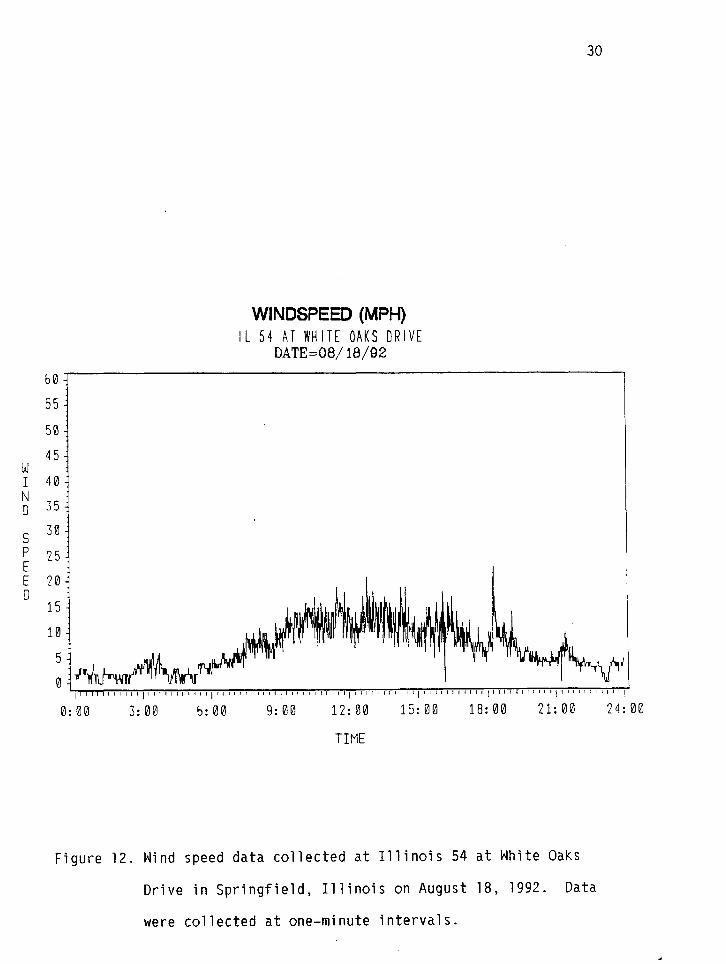
Figure 12. blind speed data collected at Illinois 54 at White Oaks
Drive in Springfield, Illinois on August 18, 1992. Data
were collected at one-minute intervals.
.

31
WINDSPEED (MPH)Il.54 AT WHITE OAKS DRIVE
DATE= 09/01/92
bO +
55{
50 {
45wI 40ND 35
~ 30
P 25EE ’20III
15{
10’ill
5
Fl
0:00 3:,00 b:OO 9:00 12:00 15:00 18:00 21:00 24:00
TIME
Figure 13. Wind speed data collected at Illinois 54at White Oaks
, Drive in Springfield, Illinois on September 1, 1992.
Data were collected at one-minute intervals.

32
WINDSPEED (MPH)l!- 54 AT WHITE OAKS DRIVE
DATE= 10/30/92
bOj
55
50
45wI 40ND 35
~ 30
P 25EE 20D
15
10
5
0
0:00 3:00 b:OO 9:00 12:00 15:00 18:00 21:00 24:00
TIME
Figure 14. Wind speed data collected at Illinois 54 at White Oaks
Drive in Springfield, Illinois on October 30, 1992.
Data were collected at one-minute intervals.

33
WINDSPEED (MPH)IL 54 AT WHITE OAKS DRIVE
DATE=ll/07/92
10:
5<
0’ 1l“’’” Ill I 11“’’’’’’’’’1’’’’’’’’’” ,l,,!l!ll!ll\-, , r 1I , l“’’’’’ ’’’’ 1’ ’’’’’’’’’’1’’” “’’”
3:00 b:OO 9:00 12:00 15:00 18:00 ?1:00 24:000:00
TIME
Figure 15. Wind speed data collected at Illinois 54at White Oaks
Drive in Springfield, Illinois on November 7, 1992.
Data were collected at one-minute intervals.
34
WINDSPEED (MPH)IL 54 AT WHIT[ OAKS DRIVE
DATE=12/22/f12
bO:
55 ~
50
D15;
10’
5{
04I1Ii11111111111811111111111111111111111111111II I l“’’’’’” “1’’’’’’’’’’’ 1’’’’’’’’’’’ 1’”” ‘“ 1, I 1I
0:00 3:00 b:OO 9:00 12:00 15:00 18:00 21:00 24:00
TIME
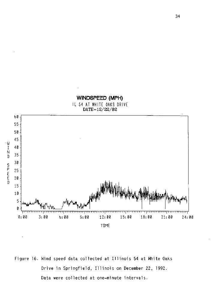
Figure 16. Wind speed data collected at Illinois 54 at White Oaks
Drive in Springfield, Illinois on December 22, 1992.
Data were collected at one-minute intervals.

35
4. STRAIN GAGE AND FREQUENCY DATA
This chapter discusses structural response data gathered during the
course of this project. Data collected included strains due to ambient
wind conditions, strain versus tip deflection, vortex shedding frequency
for ambient wind conditions, dead load strains in anchor bolts and welded
connections, and strains induced at a weld due to application of
controlled wind speeds for a cantilevered traffic signal structure.
Stresses Due to Variable S~eed Hind Loads (Ambient Winds)
A common steel traffic signal structure with a 44 foot (13.41 m)
mastarm was installed at the Physical Research Laboratory in Springfield,
Illinois in order to monitor applied stress range versus frequency of
occurrence due to ambient winds. The structure and strain gage locations
are shown in Figure 17. Strains at the exterior fillet weld connections
were measured using weldable, electrical resistance strain gages
(MicroMeasurements, Inc., Raleigh, NC, USA). Strains in the anchor bolts
were measured using bolt gages (Type BTM-6C, TML, Ltd, Tokyo, Japan) which
were installed after erection of the vertical pole. The data were
collected and processed by a Rainflow cycle counting algorithm (ASTM
EI049-85) incorporated in the SOMAT 2000 Data Acquisi
Corporation, Champaign, Illinois). The data were div
(3.45 MPa) increments for ease of handling. The resu’
ion System (SOMAT
ded into 0.5 ksi
ting stress
range-frequency data for the fillet weld connection for a four-month
period are shown in Table 4a.
There is a noticeable difference in the number of recorded stress
cycles between the top strain gage (lift) and the side strain gage
(drag). A total of 3,072,316 stress cycles were recorded for the side
gage, while only 2,448,558 stress cycles were recorded for the top gage.

36
o7 o9
0a o0
Figure 17. Instrumented traffic signal mastarm installed at Physical
Research Laboratory in Springfield, Illinois. Strain gage
locations are shown.
37
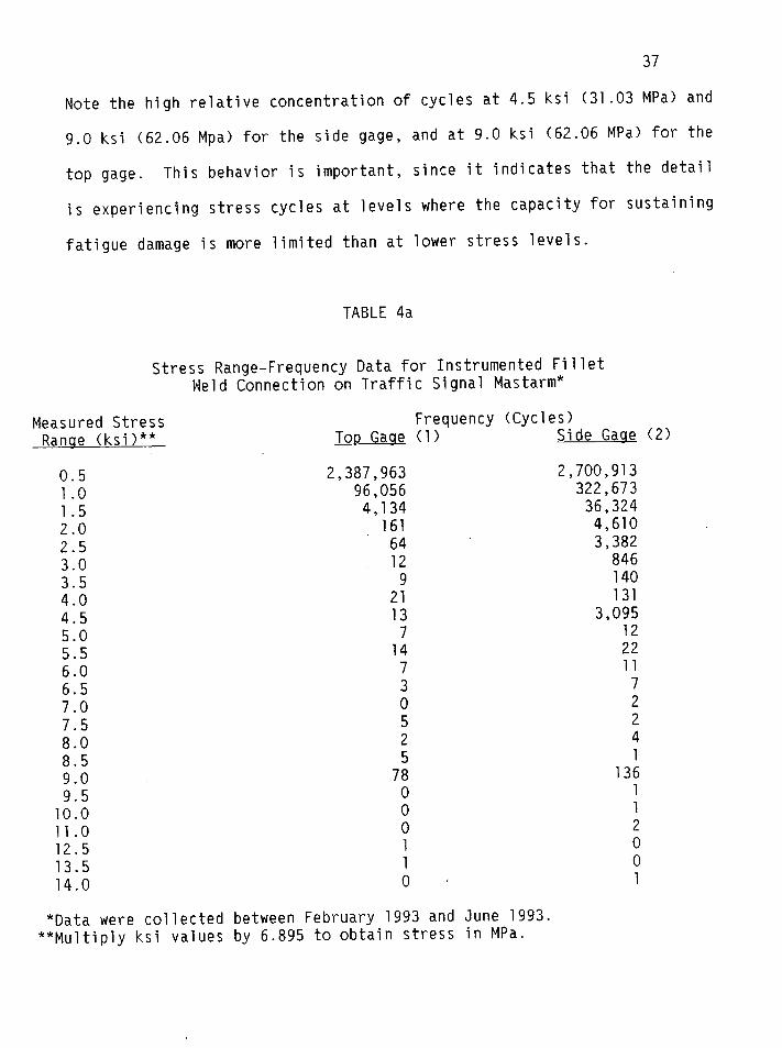
Note the high relative concentration of cycles at 4.5 ksi (31.03 MPa) and
9.0 ksi (62.06 Mpa) for the side gage, and at 9.0 ksi (62.06 MPa) for the
top gage. This behavior is important, since it indicates that the detail
is experiencing stress cycles at levels where the capacity for sustaining
fatigue damage is more limited than at lower stress levels.
TABLE 4a
Stress Range-Frequency Data for Instrumented FilletHeld Connection on Traffic Signal Mastarm*
Measured Stress Frequency (Cycles)Ranue (ksi)** TOD Gage (1) Side Gaqe (2)
0.51.01.52.02.53.03.54.04.55.05.56.06.57.07.58.08.59.09.510.011.012.513.514.0
2,387,96396,0564,134
16164129
2113714730525
78000110’
2,700,913322,67336,3244,6103,382
846140131
3,09512221172241
136112001
*Data were collected between February 1993 and June 1993.**Multiply ksi values by 6.895 to obtain stress in MPa.

38
Stress range versus frequency data for the tension dead load anchor
bolts is given in Table 4b.
TABLE 4bStress Range-Frequency Data for Instrumented Anchor Bolts
for Cantilevered Traffic Signal Structure*
Frequency (Cycles)Measured StressRanqe (ksi)** Northwest Bolt (7) Southwest Bolt (8)
0.51.01.52.02.53.03.54.04.55.05.56.06.57.07.5
:::9.09.510.010.511.011.512.012.513.013.514.014.515.015.516.016.517.017.518.018.519.0
3,536,599201,288
1,254292280137475967868492
26637
505898769
1,495503301211800211000617
4,686,39452,7481,274288376315162272
67,4245813513411250838938
2,20068375655134623123468143044142520151713
278
*Data were collected between June 1993 and November 1993.**To obtain stress in MPa, multiply ksi values by 6.895.

39
There are large discrepancies between the two sets of bolt data.
Some of this discrepancy may be attributed to wind direction effects
(prevailing southwesterly winds), which could influence the number of
tension cycles experienced. The maximum stress ranges measured for the
welds and anchor bolts are reasonable.
Dead Load Stresses Measured in Anchor Bolts and Welds
The structure was instrumented before assembly so that dead load
stresses could be determined. Measured strains for both mastarm erection
and traffic signal attachment are shown in Table 5.
TABLE 5
Measured Dead Load Strains on Traffic Signal Structure
Gage Strain Due to Strain Due toLocation
12345678910
*Units are 10-6 in/values by 30 x 106.values by 207 x 103
Mastarm*
338195
-14468106
-19416
102-44-92
Traffic Signals*
404180
-25337118
-25021123-64
-136
n. To calculate stress in psi, multiply strainTo calculate stress in MPa, multiply strain
The strains recorded do not quite conform
behavior. That is, Gages 1 and 3 are expected
strains, as are Gages 5 and 6. Gages 2 and 4,
to the generally expected
to show equal but opposite
located near the neutral
40
axis for vertical bending, should be showing more nearly zero strain. The
anchor bolt strain gages would be expected to show comparable tensile
strains in Gages 7 and 8 and comparable compressive strains in Gages 9
and 10. Some of the apparent discrepancies in these readings are
attributed to experimental errors. However, most of the difference in
expected behavior at the weld connection is attributed to the rapidly
changing strain gradient near the welds. The areas that are expected to
be in tension are in tension and the areas which are expected to be in
compression are in compression; the normally expected behavior of a
cantilever beam in pure bending is simply modified in close proximity to
the fillet welds
that the connect
really not rigid
Another factor affecting the experimental results is
on, although analyzed using cantilever assumptions, is
y fixed because of the deflection of the vertical pole
caused by the weight of the mastarm. This elastic support condition has
the effect of reducing the stress at the connection. The maximum strains
for the welds and the anchor bolts are reasonable.
Strain Versus Ti~ Deflection for Tat)ered Cantilevered Mastarm
In order to note the sensitivity of certain details, strains were
measured for a series of downward tip deflections. Strains in Gages 1, 5,
and 8 were measured for downward tip deflections of 0.5 inch (12.7 mm)
increments to a total deflection of 6.0 inches (157.4 mm). The deflection
was accomplished using a steel cable attached to the mastarm tip, and a
hand winch fastened to the back end of a 10,000 pound fork lift used as a
dead weight. Deflections were measured to the nearest 1/32 inch (0.794
mm) using a fixed steel ruler and a reference mark on the cable. Strain
versus tip deflection data are given in Table 6. The data show some
variability between deflection increments.

41
GageNumber
158
TABLE 6
Measured Strain Versus Tip Deflection
Deflection (inches)Q 0.5 1.0 1.5 2.0 2.5 3.0 3.5 4.0 4.5 5.0 5.5 6.0
Measured Strain*o 23 34 43 54 64 73 84 93 102 112 122 1330 15 20 28 35 40 44 50 58 65 67 72 790 15 16 21 27 32 38 38 45 49 53 57 61
*Strains are given in units of microstrain (10-6 in/in). To convert strainsto stress in psi, multiply strains by 30 x 106. To convert strains tostress in MPa, multiply strains by 207 x 103. To convert deflections to mm,multiply by 25.4.
Part of this variability is attributed to gusty wind conditions during the
test. Significant transverse tip deflection was noted during data
collection. Anchor bolt stresses would be affected in particular. Gage 1
(top of baseplate to mastarm weld connection) shows a sensitivity of 22
microstrain per inch deflection (0.866 microstrain per mm). Gage 5
(tension side of anchor bolt plate to vertical pole weld connection) shows
a sensitivity of 13 microstrain per inch deflection. Gage 8 (southwest
anchor bolt) shows a sensitivity of 10 microstrain per inch deflection
(0.394 microstrain per mm). An analytical check of the strain expected in
Gage 1 (due to a six-inch (152.4 mm) deflection) using a cantilevered
cylinder of equivalent stiffness indicates that the cantilever assumption
overestimated measured strains by a factor of 3.0. Thus, a static
analysis using the cantilever assumption is conservative, and cannot
accurately reflect the true state of stress due to wind loads. A finite
element analysis using springs at the support points would improve the
realism of an analytical model. However, as was seen in Chapter 2, there
are many factors which affect the behavior of a sign or signal structure,

42
and a static analysis of a dynamic problem has inherent drawbacks and
inaccuracies. Therefore, the use of static stress analysis methods for
fatigue study of overhead sign and signal structures is not recommended.
Vibration FreauencY and Dampinu for Tapered Cantilevered Mastarm
The frequency and amplitude of vertical vibration (due to vortex
shedding) of the traffic signal at the Physical Research Laboratory was
measured experimentally using an accelerometer and an oscil lographic chart
recorder. At the time of measurement, wind speeds recorded at this site
ranged from 12 - 20 mph (19.31 - 37.19 kmph). Conditions were very
gusty. It was of interest to measure the vortex shedding frequencies and
to compare these frequencies to calculated natural frequencies. Natural
frequencies were calculated for the mastarm by finite element analysis
(ALGOR). Vibration frequencies for a windspeed range of 12 - 16 mph
(19.31 - 26.75 kmph) varied between 1.8 and 2.2 Hz. Vibration frequencies
for windspeeds between 15 and 20 mph (24.14 and 37.19 kmph) ranged between
3.5 and 5.3 Hz. Calculated natural frequencies for the tapered mastarm
for the first three vertical modes were 1.06, 5.5, and 14.2 Hz
respectively. Obviously, the mastarm was vibrating in synchronization
with the first two natural modes at certain windspeeds.
The structural damping factor for the traffic signal mastarm was
measured to be ~= 0.006 using the chart recorder output and the following
relation:
2Jr~= ln(Ai/Ai+l) (12)
Where c = structural damping,Ai = vibration amplitude,Ai+l = next vibration amplitude.
As expected, the traffic signal structure is very lightly damped.

43
Controlled blind Speed Test Data
Prior to installation and instrumentation at the Physical Research
Laboratory, the traffic signal structure was shipped to Smith-Emery
Company in Los Angeles, California to undergo controlled wind speed
tests. The wind force was supplied by a blower which was set up to blow
air on the outermost traffic signal. Unfortunately, the structure is too
large to be tested with wind applied over the entire surface at any test
facility short of a large scale wind tunnel. The wind load applied by
this test was analogous to a point wind load at the outer traffic signal.
Although this loading ‘is not seen in practice, it was of interest to note
the behavior of the structure to a constant wind speed. Figures 18
through 21 show photographs of the test setup and wind application. The
instrumented section was the top fillet weld connection at the 12, 3, 6,
and 9 O’C
intervals
80.47, 96
ock positions. Strain data were collected over five minute
for wind speeds of 20, 40, 50, 60, 70, and 80mph (32.19, 64.37,
56, 112.65, and 128.74 km/hr). The wind speed for each test was
set by a hand-held anemometer held in front of the traffic signal prior to
data collection.
Collected strain data were converted to stresses. This stress data
is presented graphically in Figures 22 through 45. The direction of wind
load application was from west to east. The data are quite variable, and
indicate that even steady winds will induce variable amplitude cyclic
loading. Table 7 shows maximum, minimum, average, and range of stresses
for each strain gage for each applied wind load.
The general trend of the data in Table 7 shows an expected
in stress range with wind speed, although the increase is modest
noted in Chapter 2 that the drag coefficient for cylinders drops
ncrease
It was
to 0.3 in

44
the transitional Reynolds number regime. A similar effect was noted for
the experimental data for the west strain gage, The average strain data
from the
in-place
The resu”
The
with pub”
where CD
to width
west strain gage were used to calculate the apparent CD of the
traffic signal for each wind speed tested using equation (3).
ts are shown in Table 8.
average apparent CD is 0.39. This finding is not in agreement
ished data on drag of flat plates normal to the flow direction,
is about 1.2 at Re = 105 for a rectangular shape with length
ratio of 5:1.20 Note, however, that Re = 105 is in the .
subcritical range, while the calcu’
Reynolds number regime. Also, the
flexible mastarm which could have
ated values are for the transitional
traffic signal was mounted on a long,
nfluenced the experimental response.
Additional investigation of the in-situ estimation of drag coefficients
for traffic signals and sign panels is needed to better characterize this
behavior.

45
Figure 18. Instrumented section of traffic signal structure for controlled
wind speed tests. Testing and instrumentation were conducted at
Smith-Emery Company, Los Angeles, California. Strain ga9es were
placed at 12, 3, 6, and 9 o’clock positions near the toe of the
fillet weld.
46
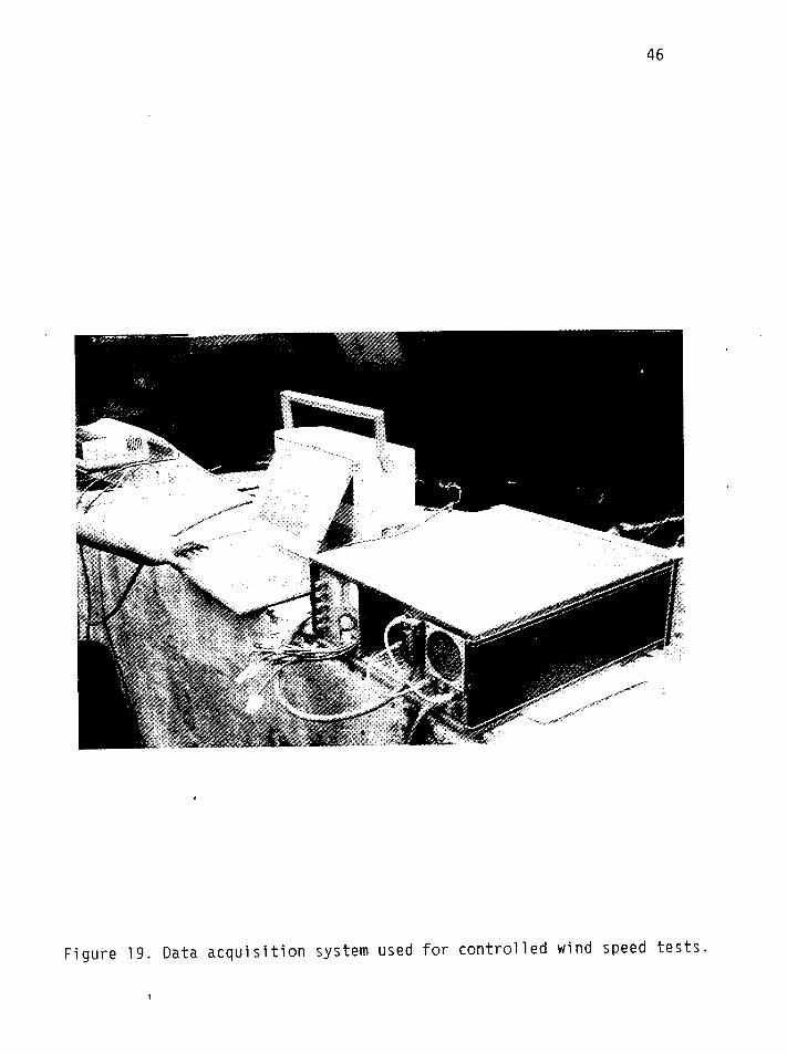
Figure 19. Data acquisition system used for controlled wind speed tests.

47
Figure 20. Equipment and setup used to apply wind loads. Technician is
checking wind speed with a hand–held anemometer.

48
Figure 21. Eighty mile per hour (133.6 kmph)wind load being applied to
traffic signal structure.

49
TABLE 7
Statistics For Controlled Wind Speed Test Data
MaximumStress (t)si)’
Lift Stresses(Top Strain Gage)Wind S~eed (m~h)**
20 -138.440 868.550 1544.560 2252.370 2113.980 2393.9
Lift Stresses(Bottom Strain Gage)Wind St)eed (mt)h)
204050607080
Drag Stresses(West Strain Gage)Wind Speed (mph)
204050607080
Drag Stresses(East Strain Gage)Wind S~eed (mDh)
204050607080
3.3869.21119.32110.21971.92251.8
3117.63982.54093.14801.24945.96783.9
994.31011.41543.51685839.11260.5
MinimumStress (~si)
-2119.9-971.6
-1003.6-720.6-434.2-154.3
-2119.8-1819.8-1570.4-1287.3-1000.8-1145.7
-4101.1-2103.9-2418.8-3268.1-2698.8-1994.2
-3251.8-2526.7-2136.9-1570.8-1425.8-1429.3 ,
AverageStress (psi)
-1210.0-6.3304.5270.1705.8995.7
-1113.2-216.1-17.6-0.6335.0545.2
644.2995.61474.41685.62814.32918.6
-697.2-733.7-421.7
86.9-152.8
-0.3
*To convert stress to MPa, multiply by 6.895 x 10⁻³.**To convert mph to km/hr, multiply by 1.67.
StressRange (psi)
1981.51840.02548.02972.92548.22548.2
2123.12689.02689.73397.52972.83397.5
7218.76086.46511.98069.47644.78778.1
4246.13538.13680.43255.92264.82689.8
Note: Data is for wind applied to a single traffic signal only, not theentire structure.

50
0
-0.2
-0.4
-0.6
~ -0.8
~ -1.2
* .1.4m
-1.6
-1.8
-2
-2.2
CONTROLLED WIND SPEED TESTLift Stresses Due to 20 Mph Wind (Top Gage)
—
—I
o I 100 I 200 I 30060 150 260
Time (see)
Figure 22. Lift stresses at top strain gage due to 20 mph (32.19 km/hr)
controlled wind application.

51
10.90.80.70.60.50.40.3
g 0.2* 0.1
~ -0.2h -0.3
-0.5
-0.6
-0.7
-0.8
-0.9
-1
-1.1
CONTROLLED WIND SPEED TESTLHt Stresses Due to 40 Mph Wind (Top Gage)
L
1 I I !o 100 200 300
50 150 250
Time (see)
Figure 23. Lift stresses at top strain gage due to 40 mph (64.37 km/hr)
controlled wind application.

52
1.8
1.6
1.4
1.2
1
- 0“8
“~ 0.6
- 0.40~ 0.2
0
6-0.2
-0.4
4.6
-0.8
-1
-1.2
CONTROLLED WIND SPEED TESTLift Stresses Due to 50 Mph Wind (’Top Gage)
I
o I 100 I 200 I 30050 150 250
Time (see)
Figure 24. Lift stresses at top strain gage due to 50 mph (80.47 km/hr)
controlled wind application.

53
2.4 —
2.2
2 –
1.8
1.6
1.4
n 1.2
‘~ , -
- 0.80u) ‘“6 ‘g 0.4 -
G 0“2 -0
4.2
-0.4
-0.6
-0.8
-1[
CONTROLLED WIND SPEED TESTLift Stresses Due to 60 Mph VVind(Top Gage)
I
o I 100 I 200 I 30050 150 250
Time (see)
Figure 25. Lift stresses at top strain gage due to 60 mph (96.56 km/hr)
controlled wind application.

54
2.4
2.2
2
1.8
1.6
n 1.4
“z 1.2*
1u)~ 0.8
a)k 0.6
G 0.4
0.2
0
-0.2
-0.4
-0.6
CONTROLLED WIND SPEED TESTLift Stresses Due to 70 Mph Wind (Top Gage)
o I 100 I 200 1’ 30050 150 2s0
Time (see)
Figure 26. Lift stresses at top strain gage due to 70 mph (112.65 km/hr)
controlled wind application.

55
CONTROLLED WIND SPEED TESTLift Stresses Due to 80 Mph Wind (Top Gage)
2’r2.4
t2.2L
- 1“6‘~ 1.4
- 1.2UJ01a)L 0.8
~ 0.6I
0.4t
0.2
0L
-0.2t
4.4 L
o I 100 I 200 I 30050 150 250
Time (see)
Figure 27. Lift stresses at top strain gage due to 80 mph (128.74 km/hr)
, controlled wind application.

56
4
3
2
1
0
-1
-2
-3
-4
-5
CONTROLLED WIND SPEED TESTDrag Stresses Due to 20 Mph Wind (West Gage)
I I I I i I [
o I 100 I 200 I 30050 150 250
Time (see)
Figure 28. Drag stresses at west strain gage (facing wind) due to 20 mph
(32.19 km/hr) controlled wind application.

57
CONTROLLED WIND SPEED TESTDrag Stresses Due to 40 Mph Wind (West Gage)
II I I Io 100 200 300
50 150 250
Time (see)
Figure 29. Drag stresses at west strain gage (facing wind) due to 40 mph
(64.37 km/hr) controlled wind application.

CONTROLLED WIND SPEED TESTDrag Stresses Due to 50 Mph Wind (West Gage)
1
%a)
6°
-1
-2
-3
0 I 100 I 200 I50
300150 250
Time (see)
Figure 30. Drag stresses at west strain gage (facing wind) due to 50 mph
, (80.47 km/hr) controlled wind application.

59
6
5
4
3
nm-
2:
01000
5-1
-2
-3
-4
CONTROLLED WIND SPEED TESTDrag Stresses Due to 60 Mph Wind (West Gage)
o I 100 I 200 I 300
50 150 250
Time (see)
Figure 31. Drag stresses at west strain gage (facing wind) due to 60 mph
(96.56 km/hr) controlled wind application.
6
5
4
3
n●9
2E
(/)1u)(BO
6-1
-2
-3
-4
CONTROLLED WIND SPEED TESTDrag Stresses Due to 70 Mph Wind (West Gage)
o I 100 I 200 I 30050 150 250
Time (see)
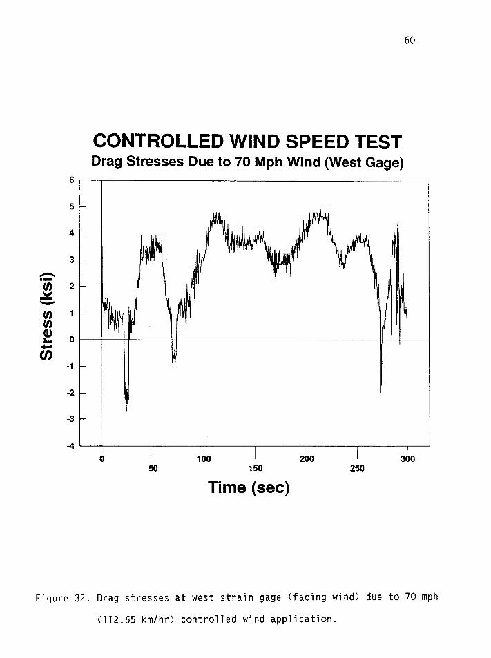
Figure 32. Drag stresses at west strain gage (facing wind) due to 70 mph
(112.65 km/hr) controlled wind application.

n●-
Su)coa)
6
8
7
6
5
4
3
2
1
0
-1
-2
-3
CONTROLLED WINDDrag Stresses Due to 80 Mph
—
o
SPEED TESTWind (West Gage)
vI
50100 I 200
150
I250
300
Time (see)
Figure 33. Drag stresses at west strain gage (facing wind) due to 80 mph
(128.74 km/hr) controlled wind application.

62
0.2
0
-0.2
-0.4
43.6
n
u)(/) -1.2
a)~ -1.4
U)-1.6
-1.8
-2
-2.2
-2.4
CONTROLLED WIND SPEED TESTLift Stresses Due to 20 Mph Wind (Bottom Gage)
I
-1
0 I 100 I 200 I 30050 150 250
Time (see)
Figure 34. Lift stresses at bottom strain gage due to 20 mph (32.19 km/hr)
controlled wind application.

63
1
0.8
0.6
0.4
0.2
no
“j -0.2
w 4.4
CfJ~ -0.6
A -0.8
3 -1
-1.2
-1.4
-1.6
-1.8
-2
CONTROLLED WIND SPEED TESTLiftStresses Due to 40 Mph Wind (Bottom Gage)
—
, I I II
o I50
100 I 200 I 300150 250
Time (see)
Figure 35. Lift stresses at bottom strain gage due to 40 mph (64.37 km/hr)
controlled wind application.

64
1.4
1.2
1
0.8
0.6
0.4
~ 0.2
*O
(/)-0.2
u)0 4“4
k -0.6(/3
-0.8
-1
-1.2
-1.4
-1.6
-1.8
CONTROLLED WIND SPEED TESTLift Stresses Due to 50 Mph Wind (Bottom Gage)
—
—
o I 100 I 200 I 30050 150 250
Time (see)
Figure 36. Lift stresses at bottom strain gage due to 50 mph (80.47 km/hr)
controlled wind application,
65
CONTROLLED WIND SPEED TESTLift Stresses Due to 60 Mph Wind (Bottom Gage)
2.4 —
2.2 –
2 –
1.8
1.6 –
1.4 –
n 1.2
“~ , .
- 0.8u)u) 0“6 –g 0.4 -
3 0“2 -0
-0.2
-0.4
-0.6
-0.8
-1 [I I I I 1
0 I 100 I 200 I 30050 150 250
Time (see)
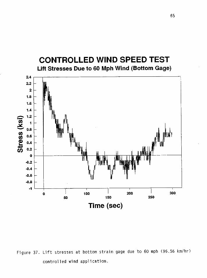
Figure 37. Lift stresses at bottom strain gage due to 60 mph (96.56 km/hr)
controlled wind application.

66
CONTROLLED WIND SPEED TESTLift Stresses Due to 70 Mph Wind (Bottom Gage)
n8-
2
2.2,
2
1.8
1.6
1.4
1.2
1I A
nd
4.2
[
‘1 , L I-0.4 !
-0.6m
‘!
1
-0.8
-1
I m
-1.2 I I I i Io 100 200 300
50 150 250
Time (see)
Figure 38. Lift stresses at bottom strain gage due to 70 mph (112.65 km/hr)
controlled wind application.
.
67
CONTROLLED WIND SPEED TESTLift Stresses Due to 80 Mph Wind (Bottom Gage)
2.6
2.4
2.2
2
1.8[
- 1“6‘ZJ 1.4
- 1.2 [
0.4
0.2
0
-0.2
4.4 I 1 ) I I
o 1“ 100 I 200 I 300
50 150 250
Time (see)
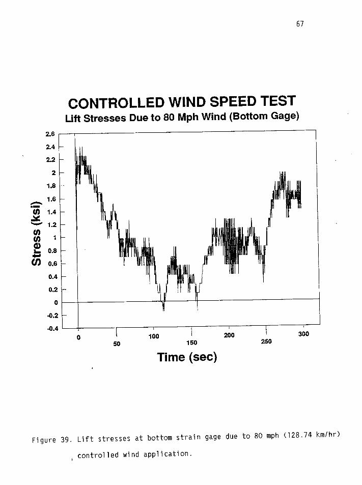
Figure 39. Lift stresses at bottom strain gage due to 80 mph (128.74 km/hr)
, controlled wind application.

68
1.5
1
0.5
0
n
“z -0.5&
(n -1u)a)k -1.5
F)-2
-2.5
4
-3.5
CONTROLLED WIND SPEED TESTDrag Stresses Due to 20 Mph Wind (East Gage)
o 1’ 100 1’ 200 1“ 30050 150 250
Time (see)
Figure 40. Drag stresses at east strain gage due to 20 mph (32.19 km/hr)
controlled wind application.

69
1.5
1
0.5
no
■-
g 4.5
u)g .,
5 -1.5
-2
-2.5
-3
CONTROLLED WIND SPEED TESTDrag Stresses Due to 40 Mph Wind (East Gage)
I
o I 100 I 200 I 300
50 150 250
Time (see)
Figure 41. Drag stresses at east strain gage due to”40 mph (64.37 km/hr)
controlled wind application.

70
2
1.5
1
n0.5
■ -
go
UJ
~ -0.5a)
G -1
-1.5
-2
-2.5
CONTROLLED WIND SPEED TESTDrag Stresses Due to 50 Mph Wind (East Gage)
o I 100 I 200 I 30050 150 250
Time (see)4
Figure 42. Drag stresses at east strain gage due to 50 mph (80.47 km/hr)
, controlled wind application.

71
2
1.5
1
~ 0.5
x
00v)a)
b -0.5m
-1
-1.5
-2
CONTROLLED WIND SPEED TESTDrag Stresses Due to 60 Mph Wind (East Gage)
I I
o I 100 I 200 I 30050 150 250
Time (see)
Figure 43. Drag stresses at east strain gage due to”60 mph (96.56 km/hr)
controlled wind application.

72
1
0.8
0.6
0.4
0.2
nm- 0
2- -0.2
CONTROLLED WIND SPEED TESTDrag Stresses Due to 70 Mph Wind (East Gage)
I
u)(/) -0.4
a)& -0.6
u)-0.8
-1
-1.2
-1.4
-1.6
0 I 100 I 200 I 30050 150 250
Time (see)
Figure 44. Drag stresses at east strain gage due to 70 mph (112.65 km/hr)
controlled wind application.

73
1.4
1.2
1
0.8
0.6
0.4
0.2
0
-0.2
-0.4
-0.6
-0.8
-1
-1.2
-1.4
-1.6
CONTROLLED WIND SPEED TESTDrag Stresses Due to 80 Mph Wind (East Gage)
—
I
—
III
I I I I I Io I 100 I 200 I 300
50 150 250
Time (see)
Figure 45. Drag stresses at east strain gage due to’80 mph (128.74 km/hr)
controlled wind application.

74
TABLE 8
Apparent Drag Coefficient for In-Place Traffic SignalUsing Average Strain Data
Wind Speed Reynolds Apparent Drag(m~h)’ Number Coefficient20 9.3 x 10⁵ 0.8640 1.8 X 10⁶ 0.3350 2.3 X 10⁶ 0.3260 2.8 X 10⁶ 0.2570 3.2 X 10⁶ 0.3180 3.7 x 10⁶ 0.24
*To convert to km/hr, multiply by 1.67.
Closure
(CD)
This chapter presented data collected during the course of this
research project for a common traffic signal structure. The structure was
installed at the Physical Research Laboratory in Springfield, Illinois.
Strain gages were mounted at weld details and inside anchor bolts. Data
collection included stress range-frequency histograms for weld detai’
the mastarm-baseplate connection and the tension dead load anchor bo’
strains due to installation of the mastarm and traffic signals; stra
s at
ts;
ns as
a function of vertical tip deflection; vibration frequency and amplitude
due to wind loads; and weld strains as a function of controlled-velocity
wind loads applied at the mastarm tip traffic signal.
The collected data showed some variability and uncertainty associated
with experimental error, difficult experimental conditions, and
differences between design assumptions and actual response. However, the
strains measured were reasonable. Observation of the data indicates that
welds and anchor bolts experience large numbers of stress cycles. The
analysis of a tapered mastarm using a cantilevered tube of equivalent

75
stiffness produces conservative stress results. Experimental results
revealed that the structure vibrated in synchronization with the first and
second natural transverse modes during wind speeds of 12 - 20 mph
(19.31 - 37. 19 kmph). The structural damping factor was measured to be
0.006, indicating light damping. The application of controlled winds to
the structure showed that even constant wind speeds produce highly
variable strain data. The reduction of the apparent drag coefficient of
an in–place traffic signal as a function of Reynolds number was noted.
The nature of wind speed variability and the variable response of a
wind-loaded structure indicate that the use of simple static analytical
methods for fatigue analysis are subject to much uncertainty. Chapter 5
presents a discussion of fatigue and outlines a fatigue analysis method
which utilizes experimental data.

76
5. DETERMINATION OF FATIGUE DAMAGE TO COMPONENTS
This chapter discusses calculation of fatigue damage. The
histogram-linear damage methodz’ is used to estimate fatigue damage and
expected fatigue life.
Overview of Fatique
Fatigue is a cumulative damage process caused by the repeated
application of loads which results in cracking or rupture of components.
‘ The danger which fatigue presents is that failures can occur at applied
stress levels much lower than the tensile strength of a given material.
Fatigue may be divided into two domains in which failure is probably
produced by different physical mechanisms. One domain, known as low-cycle
fatigue, is characterized by the application of significant plastic
strains during each load cycle. Low-cycle fatigue is associated with
lives of less than about 104 cycles. The other domain is known as
high-cycle fatigue. In this domain, cyclic strains are confined mostly to
the elastic range and result in lives in excess of about 104 cycles.
The fatigue life of a component may also be considered in two
phases. The portion of life which occurs before the appearance of a
visible crack is known as the crack initiation life. The remaining life
from crack initiation to unstable crack growth is known as the propagation
life.,
For practical purposes, especially for nonredundant components and
the types of steels generally used for sign and signal structures, the
crack propagation life of weld details is assumed to be a small fraction
of the total life. This means that the appearance of a crack indicates
that the effective fatigue life is used up. This report concentrates on
high-cycle fatigue, with failure assumed to mean crack initiation.

There are many factors which can affect the fat
component. These factors include 1) material compos
and grain direct
discontinuities,
surface stresses
77
gue life of a
tion, 2) grain size
on, 3) heat treatment, 4) welding, 5) geometrical
6) surface conditions, 7) size effects, 8) residual
9) corrosion, 10) fretting, and 11) mean stress
effects. A discussion of most of these factors is beyond the scope of
this report; however, geometrical discontinuities are discussed in a
subsequent section. Mean stress effects are discussed in Chapter 7.
The various fatigue damage theories in use assume that the
application of any cyclic stress amplitude will result in fatigue damage.
The seriousness of the fatigue damage is related to the number of applied
cycles at that stress amplitude and also to the total number of cycles
needed to produce failure of an undamaged specimen at that stress
amplitude. Fatigue damage is assumed to be permanent. Application of
several different stress amplitudes results in the accumulation of total
damage which is equal to the sum of the damage increments caused by each
applied stress level. Failure is assumed when the total damage reaches a
critical value. Many different fatigue damage theories exist. The first
cumulative damage theory proposed was attributed to Palmgren22
and
Miner, 23 and is still in wide use. This report focuses on use of the
Palmgren-Miner linear damage rule in combination with stress
range-frequency histograms to quantify fatigue damage.
Quantification of Fatique Damaqe
The Palmgren-Miner fatigue damage equation assumes a linear
relationship between number of applied stress cycles and number of stress
cycles to failure at each stress range. The ratio of applied to available
cycles at each stress range quantifies the damage. The total damage is
the sum of the damage fractions at each stress range. Failure is assumed

78
to occur when the total damage reaches unity. The relationship is shown
below in equation form:
?+ni
sri ‘1i=l
(13)
where nsri = number of applied stress cycles at the ith stressrange, ksi or MPa,
Nsri = number of available stress cycles at the ithstress range, ksi or MPa,
Nt = total number of stress ranges applied to component.
In order to determine the amount of fatigue damage suffered by a
fatigue-prone detail, a stress range-frequency histogram must be available
for the ambient stresses applied to that detail. In addition, the number
of available cycles to failure at each stress level must be known. The
American 14elding Society (A14S)publishes conservative stress range versus
frequency (S-N) curves for various categories of welded tubular
connections. 24 This data may also be expressed as a family of N-S
equations, where the number of cycles, N, is the dependent variable
instead of stress range. The equation has the form:
N = C(Sr)m (14)
where N = number of available stress cycles at stress range Sr,c = fatigue strength coefficient,m = fatigue strength exponent,Sr = stress range, ksi.
Table 9 summarizes fatigue strength coefficients and exponents for
various welded tubular steel details using the conservative data of AWS.
Stress range must be in ksi.
Applied stress ranges and frequencies may be calculated analytically
or measured experimentally. The total number of available cycles to
failure at each stress range is calculated by equation (14), and the total
damage is calculated by the Palmgrem-Miner linear damage equation (13).
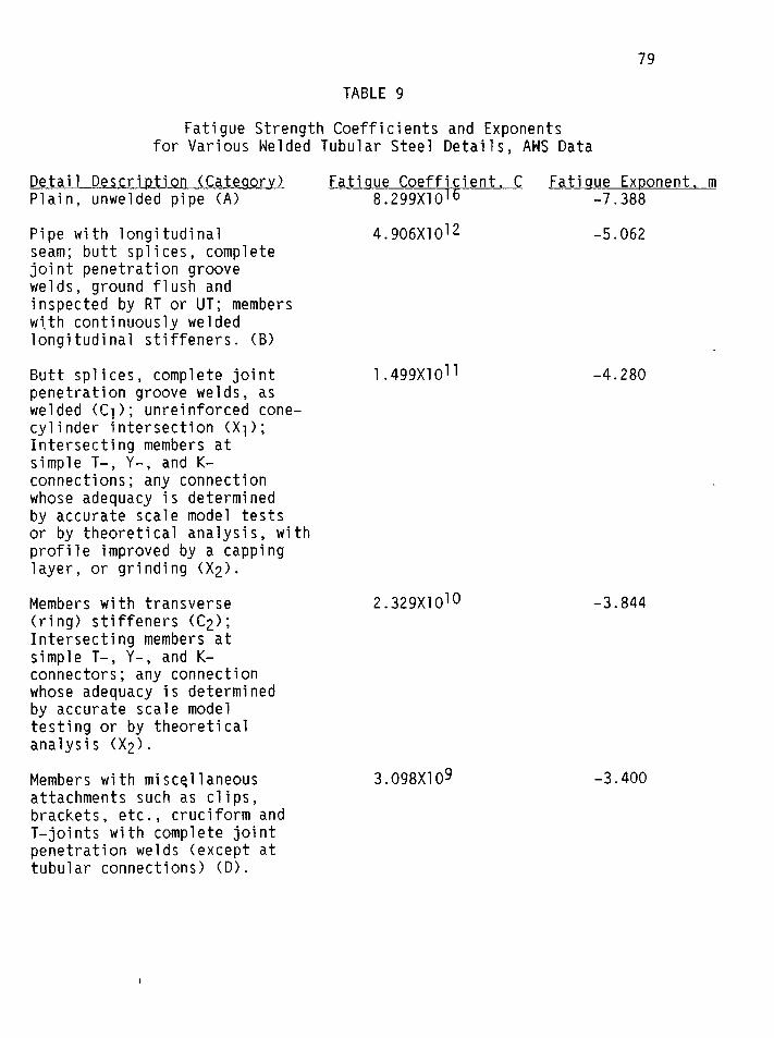
79
TABLE 9
Fatigue Strength Coefficients and Exponentsfor Various Welded Tubular Steel Details, AWS Data
Detail Descri~tion (Cateuory) Fatiuue Coefficient, C Fatique Exponent, mPlain, unwelded pipe (A) 8.299X10¹⁶ -7.388
Pipe with longitudinal 4.906X10¹² -5.062seam; butt splices, completejoint penetration groovewelds, ground flush andinspected by RT or UT; memberswi,th continuously weldedlongitudinal stiffeners. (B)
Butt splices, complete jointpenetration groove welds, aswelded (Cl); unreinforced cone-cylinder intersection (Xl);Intersecting members atsimple T–, Y–, and K-connections; any connectionwhose adequacy is determinedby accurate scale model testsor by theoretical analysis, withprofile improved by a cappinglayer, or grinding (X2).
Members with transverse(ring) stiffeners (C2);Intersecting members atsimple T-, Y–, and K-connectors; any connectionwhose adequacy is determinedby accurate scale modeltesting or by theoreticalanalysis (X2).
Members with miscellaneousattachments such as clips,brackets, etc., cruciform andT-joints with complete jointpenetration welds (except attubular connections) (D).
1.499X10¹¹
2.329X10¹⁰
3.O98X1O9
-4.280
-3.844
-3.400

80
TABLE 9 (Continued)
Detail Descri~ tion (Cateaorv) Fatiaue Coefficient. C Fatiaue Ex~onent, m
Balanced cruciform and T- 1.27OX1O9 -3.254joints with partial jointpenetration groove weldsor fillet welds (except attubular connections);members where doubler wrap,coverplates, longitudinalstiffeners, gusset plates,etc. , terminate (exceptat tubular connections) (E).
End weld of coverplate ordoubler wrap; welds ongusset plates, stiffeners,etc. , cruciform and T-joints,loaded in tension or bending,having filled on partial jointpenetration-groove welds(except at tubular connections) (F).
2.168X10¹³
Connections designed as 9.148X10⁹simple T-, Y-, or k-connections with completejoint penetration groovewelds meeting prequalificationrequirements of AWS D1.1 - 84Figure 10.13.1A (DT).
Simple T-, Y-, and K-connections with partialjoint penetration groovewelds or fillet welds;complex tubular connectionsin which the punching shearcapacity of the main membercannot carry the entire loadand load transfer isaccomplished by overlap,gusset plates, ring stiffeners,etc. (ET).
Simple T-, Y-, or k-connections loaded intension or bending, havingfillet or partial jointpenetrating groover welds(shear stress in welds) (FT).
1.OO3X1O8
-7.050
-4.691
-3.393
2.303X10¹¹ -7.246(stress range less than 5.5 ksi [37.9 MPal)1.468X10⁹ -4.306(stress range greater than 5.5 ksi [37.9MPal)

81TABLE 9 (Continued)
Detail Descri~tion (Cateuorv) Fatigue Coefficient, C Fatiuue Exponent. m
Simple T-, Y-, and k- 2.701X10⁷ -4.281connections in whichthe gamma ratio of mainmember does not exceed 24 (K2).
Same as above with profile 6.276X10⁷ -4.397improved per AWS D1.1-8410.7.5 (Kl).
*For more complete descriptions of these detail categories, see AWS D1.1-84Table 10.7.3.
If the stress range-frequency histogram is calculated or measured for
a year-long period, the expected fatigue life of the detail is simply
calculated by:
L=~ (15)D
Where L = expected fatigue life of detail, years, andD = total damage caused by stress range-frequency
histogram.
One should be aware of the possible variation of wind speeds at a
specific site from year to year. If a five-year histogram were
constructed from local weather station data, the fatigue life estimation
equation would return life (L) as the expected number of five-year loading
blocks.
Anchor Bolts
Anchor bolts may also be analyzed for fatigue using the same basic
N-S equation. Fatigue strength coefficients and exponents vary with
material and type of fatigue test (i.e. notched or unnotched). Steels
commonly used in anchor bolts have similar tensile and physical properties
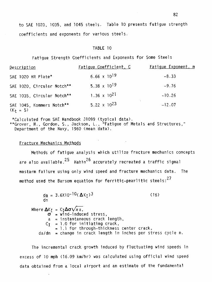
82
to SAE 1020, 1035, and 1045 steels. Table 10 presents fatigue strength
coefficients and exponents for various steels.
TABLE 10
Fatigue Strength Coefficients and Exponents for Some Steels
Description Fatiaue Coefficient. C Fatiaue Ex~onent, m
SAE 1020 HR Plate* 6.66 x 10¹⁹ -8.33
SAE 1020, Circular Notch** 5.38 X 10¹⁹
SAE 1035, Circular Notch** 1.36 X 10²¹
SAE 1045, Kommers Notch** 5.22 X 10²³(Kt = 5)
-9.76
-10.26
-12.07
*Calculated from SAE Handbook J1099 (typical data).**Grover, H., Gordon, S., Jackson, L., “Fatigue of Metals and Structures,”
Department of the Navy, 1960 (mean data).
Fracture Mechanics Methods
Methods of fatigue analysis which utilize fracture mechanics concepts
25are also available. Hahin26 accurately recreated a traffic signal
mastarm failure using only wind speed and fracture mechanics data. The
method used the Barsom equation for ferritic-pearl itic steels:27
a= 3.6X10⁻¹⁰(AK1)3 (16)dn
blhereAKI = cIAcJfio = wind-induced stress,
= instantaneous crack length,c; = 1.0 for initiating crack,
1.1 for through-thickness center crack,da/dn ~ change in crack length in inches per stress cycle n.
The incremental crack growth induced by fluctuating wind speeds in
excess of 10 mph (16.09 km/hr) was
data obtained from a local airport
calculated using official wind speed
and an estimate of the fundamental
83
frequency. The incremental increase, da, was added to the existing crack
length, a, and this new crack length was used in the equation above. A
daily record of the crack length progression was constructed, and fatigue
transition-to-overload was predicted with less
the actual failure history.
The context of this application was a fai
initial and final transition-to-overload (crit
than 12% error compared to
ure analysis. As such, the
cal) crack lengths were
known. The accuracy of fracture mechanics methods depends strongly on
knowledge of initial defect size, and has a weaker dependence on critical
crack size. The initial defect used in Hahin’s analysis was a 2.54-inch
(64.5 mm) long, 0.057-inch (1.45 mm) deep fingernail crack which was
probably popped-in during erection of the structure. The structure failed
catastrophically after five months of service. This rapid failure
reinforces the assumption that most of the fatigue life of a weldment is
taken up by the crack initiation process.
Stress Concentration Effects
The simple formulas used for stress calculations in design are based
on constant or slowly varying member cross sections. When these
conditions are not met, such as in the presence of shoulders, grooves,
holes, threads, and other sharp discontinuities, the simple stress
distributions are modified so that localized high stresses occur. The
localization of high stresses is known as a stress concentration, and is
measured by the stress concentration factor, defined as:
Kt =~max/~nom (17)
Where ~max = maximum stress at region of interest, andOnom s nominal stress in region of interest.

84
The subscript ‘t’ indicates that the stress concentration factor is
obtained from theoretical analysis, usually based on assumptions common in
theory of elasticity (Hooke’s law, homogeneity, etc.). Stress
concentration factors are also obtained experimentally by means such as
photoelasticity and precision strain gages. When experimental work is
sufficiently precise, excellent agreement is obtained with
well-established mathematical results.
The impact of stress concentrations on fatigue analysis is that
nominal section stresses are magnified at sharp section changes by a
factor that can range from 1.10 to about 10 in extreme cases. Because the
histogram linear damage method uses stresses to calculate the number of
available cycles, an underestimation of actual stress at the detail of
interest will result in a higher number of available cycles. This results
in a lower damage fraction for a given number of applied cycles and,
consequently, a longer expected fatigue life.
The most common sites of stress concentration in overhead sign and
signal supports are at welds and anchor bolts. Stress concentration
factors for fillet welds may be estimated by treating the connection as a
stepped round shaft in tension or bending with a certain fillet radius and
by using appropriate published stress concentration curves. Anchor bolts
may be considered as grooved shafts in tension. Several reference books,
such as Peterson,28
are available to quantify stress concentration
factors for various geometries. Figures 46 and 47 show graphs of stress
concentrations for the details mentioned above.
Current design specifications only address the issue of stress
concentrations in the corners of poly-sided tubes. The influence of

85
stress concentrations in weld design is restricted to reference in notes
2, 3, and 4 of Table 10.7.3 in AWS D1.1-84 - Structural Welding Code,
Steel, 1984. The stress concentration effect is predicted by theory and
proven by experiment, and should be explicitly included in both static and
fatigue analysis.
Closure
The discussion in this chapter shows how to quantify fatigue damage
to a structural detail. The histogram-linear damage method is very
straightforward to use and results in a rational fatigue damage analysis.
There are no statistical parameters to evaluate, as.in other fatigue
analysis methods, so no accuracy is lost. The method is based on the
Palmgren-Miner linear fatigue damage theory, with stress ranges and number
of applied stress cycles supplied by a stress-range frequency histogram,
and the number of available stress cycles calculated from published stress
range–cycles to failure data. Individual damage fractions at each stress
range are summed to quantify the total damage. If the histogram data
represents one year of loading, the inverse of the total fatigue damage is
the expected fatigue life of the detail in years. If the histogram data
represents a multi-year load history, the inverse of the total fatigue
damage is the expected fatigue life of the detail in terms of the
multi-year blocks used. The remaining fatigue life is the expected life
minus the number of years in service.
Stress concentration effects were discussed because of their
influence on localization of fatigue damage and on fatigue life. Proper
use of stress concentration factors in both static and fatigue design will
result in an increased accuracy of the design, and also in increased
fatigue life of the structure.
The following chapter uses the fatigue damage methods discussed here
in a sample calculation.

30
86
Figure 46. Stress concentration factor, Kt,for a stepped, round bar with
28 (Stressa shoulder fillet in bending, from Peterson
Concentration Factors, R. E. Peterson,Miley, New york~ 1g74-
Reprinted by permission of John Wiley & Sons,Inc.)

87
Figure 47. Stress concentration factor, Kt, for a grooved shaft in
tension, from Peterson28
(Stress Concentration Factors,
R. E. Peterson, Wiley, New York, 1974. Reprinted by permission
of John Wiley & Sons, Inc.) .

886. SAMPLE FATIGUE DAMAGE ANALYSES USING BOTH STRAIN GAGE
AND ANALYTICAL METHODS
The purpose of this chapter is to use the methods outlined in
Chapters 2 and 5 to es
example overhead traff
example to the reader,
imate the expected fatigue life of a part”
c signal structure. This chapter is prov
and should be considered as such.
cular
ded as an
The structure to be analyzed is a 44 foot long (13.41 m) traffic
signal mastarm, the minimum (tip) diameter is four inches (101.6 mm), the
. maximum (at the weld) diameter is ten inches (254 mm). The detail to be
analyzed is the fillet weld connecting the mastarm to the attachment ‘
plate. The fillet weld is assumed to be AWS category ET. This structure
was shown in Figure 17. The strain gage histogram linear damage method is
used first.
Analysis Usinu Strain Gage Histouram Data
The stress range-frequency data for Gage Two (Table 4a) are
used to estimate the expected fatigue life of the weld detail. Since
data were collected for four months, a reasonable estimated stress
range-frequency histogram for a one year period is made by multiplying
the number of cycles by three (3). The equation relating stress
range to
N=l .003X’
Table 11
available number of cycles for a category ET weld detail is
08(Sr)-3”3g3. Calculat ons and results are given in
TABLE 11Expected Fatigue Damage Calculation for Traffic Signal Mastarm
U~ing Strain Gage Data
Measured Applied Cycles Available DamageStress Range for 1 year cycles Fraction
(ksi)* (nsri)** (Nsri) (nsri/Nsri)
0.5 , 8.103X10⁶ 1.O54X1O9 0.00771.0 9.680X10⁵ 1.OO3X1O8 0.00971.5 1.O9OX1O5 2.534X10⁷ 0.0043

89
TABLE 11 (Continued)
MeasuredStress Range
(ksi)*
0.52.53.03.54.04.55.05.56.06.57.07.58.08.59.09.510.011.014.0
Applied Cyclesfor 1 year
(n~ri)**
8.103X1O61.OI5X1O4
2538420393
92853666332166123
4083363
AvailableCycles(Nsri)
1.O54X1O94.478X1062.412X1061.43OX1O69.O89X1O56.O95X1O54.263X1053.O85X1O52.296X1051.75OX1O51.361X1051.O77X1O58.652X1047.O43X1O45.802X1044.829X1044.O58X1O42.937X1041.296X104
Total Damage (D) =-
DamageFraction(nsri/Nsri)
0.00770.00230.00110.00030.00040.01520.00010.00020.00010.00014X10-55X1O-50.00014X1O-50.00076X10-57X1O-50.00020.0002
0.05066
*To convert to MPa, multiply by 6.895.**Data from Table 4a, Gage 2, multiplied by 3 to approximate one year period.
The expected fatigue life of the detail is calculated by equation
(15): L=l/D=l/O.05066=19.74 years. This correlates with many actual
fatigue failures of light poles and highmast structures using weathering
steel . It is interesting to note that 30% of the fatigue damage is caused
by cycling at the 4.5 ksi (31.03 MPa) stress range. The procedures
outlined above in Table 11 allow a direct, rapid quantification of fatigue
damage for a given weld detail. Because actual measured stress ranges and
frequencies were used in the calculations, the analysis is also as
accurate as possible given the statistical nature of fatigue data. An
estimate of the remaining fatigue life of the detail is obtained by
subtracting the number of years of service from the expected life. This
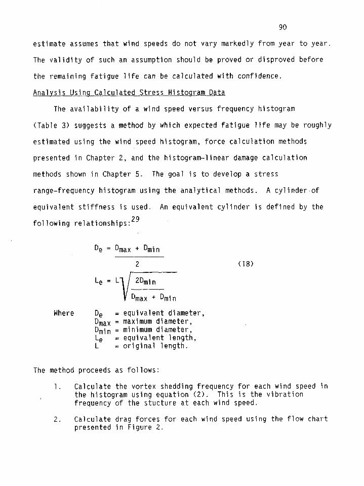
90
estimate assumes that wind speeds do not vary markedly from year to year.
The validity of such an assumption should be proved or disproved before
the remaining fatigue life can be calculated with confidence.
Analysis Usinq Calculated Stress Histoqram Data
The availability of a wind speed versus frequency histogram
(Table 3) suggests a method by which expected fatigue life may be roughly
estimated using the wind speed histogram, force calculation methods
presented in Chapter 2, and the histogram-linear damage calculation
methods shown in Chapter 5. The goal is to develop a stress
range-frequency histogram using the analytical methods. A cylinderof
equivalent stiffness is used. An equivalent cylinder is defined by the
following relationships: 29
De = Dmax + Dmin
2I
(18)
Le=L
v
2Dmin
Dmax + Dmin
Where De =Dmax =Dmin =Le =L =
equivalent diameter,maximum diameter,minimum diameter,equivalent length,original length.
The method proceeds as follows:
1. Calculate the vortex shedding frequency for each wind speed inthe histogram using equation (2). This is the vibrationfrequency of the stucture at each wind speed.
2. Calculate drag forces for each wind speed using the flow chartpresented in Figure 2.

91
3. Using the drag forces, calculate the applied stresses at thedetail(s) of interest. Total force F equals FD x Le foreach windspeed. Applied moment M equals F x Le/2 at theweld. Nominal bending stress at the weld, ~nom equals Me/I.Maximum bending stress aequals Kt xanom.
4. Assume the counts in the histogram to be one-second intervals ofconstant wind speed application; then the histogram frequencyrepresents the total number of seconds of application of aparticular wind speed. Multiply the number of seconds by thevortex shedding frequency to estimate the total number ofapplied cycles at each wind speed for a year.
5. Use the results from steps 3 and 4 to construct a new histogramfor each detail of interest. The result is a stress versus ‘cycles-per-year histogram.
6. Use the histogram developed above in conjunction with themethods outlined in Chapter 5 to calculate the expected fatiguelife of the detail(s) of interest.
Estimates of several parameters are needed in order to estimate the .
expected fatigue life analytically. These estimates are given in Table 12.
The first step in the analysis is to determine the wind speeds at
which synchronization is expected. The results of this calculation are
shown in Table 13. The criteria used for synchronization are 0.6=
fn/fss 1.4 and reduced damping (dr)<64.
Use the reduced damping (dr) from equation (8), the mode factors
(Y) for each transverse vibration mode from Table 2, and the Strouhal
Number (S) to calculate Ay/D for each mode using equation (10).
Amplified drag coefficients are then calculated from equation (4).
One is now ready to calculate drag stresses due to each wind speed
experienced. Results are shown in Table 14.

92
TABLE 12
Parameters Used For Analytical Fatigue Life Estimation
Equivalent pole diameter (De) = 0.583 ft. (0.178 m)Equivalent pole length (Le) = 33.25 ft. (10.13 m)Wall thickness (t) = 0.20 in. (5.08 mm)Elastic Modulus (E) = 30XI06 psi (207 GPa)Moment of Inertia at Weld (I=mR3t) = 24.7 in.4 (5.93X10⁻⁵ mm4)Fluid density (P) = 0.002378 slug/ft3 (9.85X10⁻⁴ kg/m3)Kinematic Viscosity (v) = 1.564X10⁻⁴ ft2/sec. (1.681X10⁻³m2/sec.)Structural Damping (~) = 0.006Mass per unit length (m) = 0.449 slug/ft (21.49 kg/m)Stress concentration factor (Kt) = 2.2First transverse mode fundamental frequency (fn~) = 1.705 HzSecond transverse mode fundamental frequency (fn2) = 10.66 HzThird transverse mode fundamental frequency (fn3) = 29.87 HzDimensionless mode factor (Vi) = 1.305Dimensionless mode factor (V2) = 1.499Dimensionless mode factor (v3) = 1.537Strouhal number (S) = 0.2Reduced Damping (~r) = 34.9
TABLE 1314indSpeeds at 14hich Synchronization is Expected
Wind Speed(mph)*
1234567891011121314151617
Reynolds Vortex SheddingNumber** Frequency (Hz) fnl/fs*** fn2/fs*** fn3/fs***
5.5X1031.1X1041.6X1042.2X1042.7X1043.3X1043.8X1044.4X1044.9X1045.5X1046.0X1046.6X1047.1X1047.7X1048.2X1048.7X1049.3X104
0.51.01.5 1.142.0 0.852.5 0.683.03.54.04.55.05.56.06.57.07.58.08.5
1.331.25

93
TABLE 13 (Continued)
Wind Speed Reynolds Vortex Shedding(mph)* Number” Frequency (Hz)-
18192021222324252627282930313233343536373839404142434445464860
9.8X1041.O4X1O51.O9X1O51.15X1051.2OX1O51.26X1051.31X1051.37X1051.42X1051.48X105I.53X1051.59X1051.64X1051.7OX1O51.75X1051.80X1051.86X1051.91X1051.97X1052.O2X1O52.O8X1O52.13X1052.19X1052.24X1052.3OX1O52.35X1052.41X1052.46X1052.52X1052.62X1053.28X105
9.09.510.010.511.011.512.012.513.013.514.014.5 ,15.015.516.016.517.017.518.018.519.019.520.020.521.021.522.022.523.023.524.0
fnl/fs*** fn2/fS*** fn31fs***
1.181.121.071.020.970.930.890.850.820.790.760.740.710.690.670.65 .0.630.61
1.391.361.331.301.271.24
*To convert to km/hr, multiply by 1.67.**Reynolds number is for the equivalent cylinder.
***Only those frequency ratios contained in the lock-in band are shown.
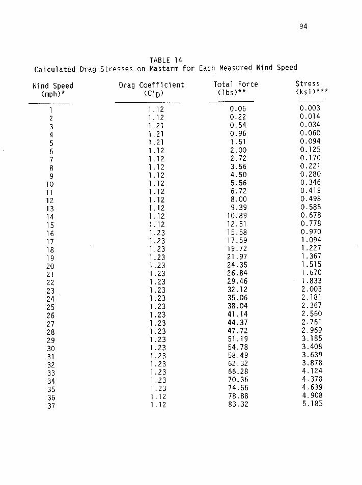
94
TABLE 14Calculated Drag Stresses on Mastarm for Each Measured Wind Speed
Wind Speed(mph)*
Drag Coefficient(c’D)
Total Force(lbs)**
1
2345678910111213141516171819202122232425262728293031323334353637
1.121.121.211.211.211.121.121.121.121.121.121.121.121.121.121.231.231.231.231.231.231.231.231.231.231.231.231.231.231.231.231.231.231.231.231.121.12
0.060.220.540.961.512.002.723.564.505.566.728.009.3910.8912.5115.5817.5919.7221.9724.3526.8429.4632.1235.0638.0441.1444.3747.7251.1954.7858.4962.3266.2870.3674.5678.8883.32
Stress(ksi)***
0.0030.0140.0340.0600.0940.1250.1700.2210.2800.3460.4190.4980.5850.6780.7780.9701.0941.2271.3671.5151.6701.8332.0032.1812.3672.5602.7612.9693.1853.4083.6393.8784.1244.3784.6394.9085.185

95TABLE 14 (Continued)
Wind Speed(mph)*
Drag Coefficient(CD)
Total Force(lbs)*
Stress(ksi)***
3839404142434445464860
1.121.121.121.121.121.231.231.231.231.231.23
87.8992.5797.38102.31107.36112.54117.83123.25128.79140.23219.11
5.4695.7606.0596.3666.6817.0027.3327.6698.0148.72613.634
*To convert to km/hr, multiply by 1.67.**To convert pounds (lbs) to Newtons (N), multiply by 4.45.
***Stress values include estimated Kt = 2.2. To convert to MPa,multiply by 6.895.
The stresses due to each wind speed have now been calculated. Steps
1 through 3 of the analytical method outlined above are complete. Step 4
is concerned with relating the shedding frequency for each wind speed to
the collected wind speed data. Results from Steps 4 through 6 are shown
in Table 15.
TABLE 15Expected Fatigue Damage Estimation Using Measured Wind Speed Data
WindSpeed(mph)*
Stress atWind Speed(ksi)**
Stress CyclesExperienced(nsri)
1
2345678910111213141516171819
0.0030.0140.0340.0600.0940.1250.1700.2210.2800.3460.4190.4980.5850.6780.7780.9701.0941.2271.367
23582.35X1045.O9X1O48.38X1041.14X1051.4OX1O51.52X1051.62X1051.62X1051.54X1051.48X1051.34X1051.19X1051.06X1059.14X1047.87X1046.48X1045.39X1044.42X104
AvailableStress Cycles
(Nsri)
2.25X10162.03X10149.93X10121.41X10123.1OX1O111.19X10114.18X10101.68X101O7.54X1093.67X1091.93X1091.O7X1O96.22X1083.77X1082.35X1081.11X1087.38X1075.O1X1O73.47X107
DamageFraction(nsri/Nsri)
1.1X1O-131.2X1O-105.1X1O-96.0X10-83.7X1O-71.2X1O-63.7X1O-69.7X1O-62.2X1O-54.2X10-57.7X1O-51.3X1O-41.9X1O-42.8X10-43.9X1O-47.1X1O-48.8X1O-41.1X1O-31.3X1O-3
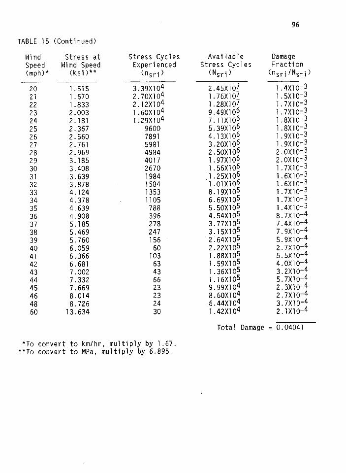
TABLE 15 (Continued)
Wind Stress atSpeed Wind Speed(mph)* (ksi)**
20 1.51521 1.67022 1.83323 2.00324 2.18125 2.36726 2.56027 2.76128 2.96929 3.18530 3.40831 3.63932 3.87833 4.12434 4.37835 4.63936 4.90837 5.18538 5.46939 5.76040 6.05941 6.36642 6.68143 7.00244 7.33245 7.66946 8.01448 8.72660 13.634
Stress CyclesExperienced
(nsri)
3.39X1042.70X1042.12X1041.60X1041.29X104
96007891598149844017267019841584135311057883962782471566010363436623232430
AvailableStress Cycles
(Nsri)
96
DamageFraction(nsri/Nsri)
2.45X1071.76X1071.28XI079.49X1067.11X1065.39X1064.13X1063.20X1062.5OX1O61.97X1061.56X106.I.25X1061.O1X1O68.19X1056.69X1055.5OX1O54.54X1053.77X1053.I5X1052.64X1052.22X1051.88X1051.59X1051.36X1051.16X1059.99X1048.6OX1O46.44X1041.42X104
1.4X1O-31.5X1O-31.7X1O-31.7xlo-31.8X10-31.8X10-31.9XI0-31.9X1O-32.OX1O-32,OX1O-31.7X1O-31.6X10-31.6X10-31.7X1O-31.7X1O-31.4X1O-38.7X10-47.4X1O-47.9X1O-45.9X1O-42.7X10-45.5X1O-44.OX1O-43.2X10-45.7X1O-42.3X10-42.7X10-43.7X1O-42.1X1O-4
Total Damage = 0.04041
*To convert to km/hr, multiply by 1.67.**To convert to MPa, multiply by 6.895.
97
The expected fatigue life is 24.75 years. Note that all of the
significant damage was due to wind speeds between 16 and 27 mph (26.72
and 43.45 km/hr). These winds correspond to the high end of the
subcritical Reynolds number range, and also to synchronized vibration
with the second natural frequency. The amplification of drag
coefficient resu
to failure. The
maximum, were st
ted in higher stresses, and thus lower available cycles
number of stress cycles experienced, while not the
11 on the order of 104 cycles. The combination led
to significant fatigue damage.
Analvsis Using AASHTO Formula
A fatigue analysis method which uses the static pressure equation
(see equation [111) was also investigated. In the AASHTO method, drag
coefficient isa function of Reynolds number, and is a constant in this
example until wind speeds of about 55 mph (91.85 kmph). The gust factor
was not used. The same histogram developed for the wind speed data
(which included synchronization effects) and the same value of Kt
resulted in an expected
to 524 years without us’
shedding effect, and us
fatigue life of 36.1 years. This life increases
ng Kt in the analysis. Neglecting the vortex
ng only the first fundamental frequency to
develop the histogram results in an expected fatigue life of 277.9
years. These results show that static methods overestimate the expected
fatigue life of a given detail by a significant margin.
Closure
Sample calculations of fatigue damage and expected fatigue life
using both collected stress range-frequency data and analytical
estimates of wind–induced stresses were presented in this chapter. The
analytical procedure overestimated the expected fatigue life by about

98
25 percent compared to the strain gage data method. Results from static
force methods were presented. These estimates of expected fatigue life were
much higher (less conservative) than those previously calculated. This an
indication that static methods are unsuitable for fatigue analysis of
overhead sign and signal structures. As stated in the chapter introduction,
the calculations are provided as examples. Other stress analysis methods
are available, the goal of any method used is to derive a reasonable stress
range–frequency histogram for use in the damage calculation procedure.

7.
99
FACTOR OF SAFETY EQUATIONS FOR FATIGUE DESIGN
The purpose of this chapter is to discuss factor of safety
equations for fatigue loaded details. Factor of safety equations are
commonly used in machine design. The purpose for calculating a factor
of safety in the context of fatigue of weldments is to determine
susceptibility to fatigue failure during the design of a welded
structure.
Factor of safety equations relate applied and mean stresses to
material propert
ultimate tensile
into a factor of
es, typically fatigue strength and either yield or
strength. The need to incorporate mean stress effects
safety for welds may be questioned by some researchers
who note that residual stresses at the weld are unpredictable, but are
generally assumed to be at or near material yield strength. Further
loading would not increase local stresses significantly due to the
plastic nature of the stress-strain response after yield.
However, welds are only part of a total structure. Cracks must
generally grow into unwelded parts of a structure in order to produce
rupture. Outside the heat affected zone, fatigue behavior is comparable
to unwelded specimens. Mean stress does affect the fatigue life of
unwelded specimens and, therefore, will influence overall structural
safety.
Factor of Safety Equations
The Goodman, Soderberg or Gerber fatigue failure equations are
commonly used to calculate the safety factor in engineering fatigue and
machine design. 30 The Goodman equation is conservative and is the

100
most widely used. The Gerber equation most accurately represents actual
experimental fatigue data. The Soderberg equation is highly
conservative. The Goodman and Gerber equations are presented below:
Goodman: N= 1
[+] [Y]S+se u
Gerber: N= 1
[ 1[dSa+Squ
Where N =Sa =Sm =se =Su =
(19)
(20)
Safety factor,alternating stress amplitude,mean stressfatigue strength of a given number of cycles, andminimum specified ultimate tensile strength.
Welded structure design codes
various details and stress ranges
amplitudes. Mean stress is a comb
stresses. The Gerber equation may
use a fatigue strength category for .
nstead of alternating stress
nation of live load and dead load
be modified to incorporate the detail
fatigue strength and the applied stress range: 31
(21)
Where SLL = live load stress range,SDL = dead load stress in weld:Fd = fatigue strength of detail at 2X10⁶ or
107 cycles,Su = minimum tensile strength of the steel specified.
In this equation, the live load stress range replaces the
alternating stress amplitude, the detail fatigue strength replaces fatigue
strength, and the mean stress component is replaced by a combination of
dead loa~ and live load stresses. Emphasis is placed on the relationship
between the live load stress range and the detail fatigue strength. The
squared term is
structure, and
101
related to the ambient dead load stress in the
s a measure of the remaining elastic-plastic strain
capacity. The squared term becomes significant when ambient stresses
start to approach code-allowable stresses. The squared term is also
significant when steels with lower notch plasticity such as ASTM A514,
A588, or A572 are used or for lower strength steels like ASTM A36 when
used at lower temperatures.
For design purposes, a safety factor range of 1.40-1.60 is
recommended when using 5(M mean fatigue data. This range takes material
and load variations into account. A safety factor as low as 1.20 may be
used when using the more conservative ANS fatigue category data. In
either case, a calculated factor of safety less than 1.00 indicates
serious potential fatigue problems.
Closure
The use of a factor of safety provides an important, useful tool
for the designer. With it, an estimate of the fatigue susceptibility of
a structural detail may be made during the design process. This allows
a fatigue-prone detail to be modified before it is placed in service.
This capability for explicitly quantifying the factor of safety is
absent from current design codes and specifications. Appropriate use of
a factor of safety for fatigue design will result in improved fatigue
life of overhead sign and signal structures because of the explicit
relationship defined between live load stress range and the fatigue
strength of the detail under consideration.

102
8. SUMMARY
The main purpose of this report was to combine pertinent wind
loading and vibration theory, fatigue damage theory, and experimental
data into a useable fatigue analysis method for overhead sign and signal
structures.
Vibrations and forces induced by vortex shedding were studied
analytically and measured experimentally. The force analysis methods
are complex and approximate because vortex shedding is an aerodynamic
behavior. Drag coefficients, generally assumed to be constants or
simple functions of Reynolds number, actually depend on the amplitude
vortex shedding vibration. This is an outcome of the dynamic
of
interaction of the fluid and the structure. The amplification of drag
coefficients can have a significant effect on resulting forces.
Although the analysis can be complex, it is preferred to static methods
for fatigue analysis purposes because of greater expected accuracy.
Fatigue and the concept of fatigue damage quantification were
discussed. Fatigue was described as a failure mode which results from
cyclic application of stresses which may be much lower than the yield
stress. The failure process, although not completely understood, can be
regarded as having two phases; crack initiation and crack propagation.
For the materials and stresses generally expected
signal structures, the crack initiation phase dom
life. Fatigue damage was quantified using the Pa’
in overhead sign and
nates the fatigue
mgren–Miner linear
damage equation. This equation relates applied stress cycles to
available stress cycles for each stress range encountered by the
detai 1. Applied stress cycles are estimated by creating a stress

103
range-frequency histogram either by analytical process or by strain
gage instrumentation of a detail in question. Available stress cycles
for each applied stress range are calculated by expressing published S-N
fatigue data for welds or anchor bolts as N-S equations, where number of
available cycles ~
range. The total
cycles to availab”
N) is the dependent variable, instead of stress
damage is the sum of the ratios of applied stress
e stress cycles. If the total damage is calculated
for a year, the inverse of the damage is the expected fatigue life in
years. The remaining life of an in-service structure is the difference
between expected life and years in service. The use and limitations of
fracture mechanics methods were discussed. Stress concentrations were
discussed as a vital parameter in fatigue analysis. Methods for
estimating Kt for fillet welds and anchor bolt threads were extracted
from the literature.
Experimental data were collected for a representative traffic
signal structure. This data included stress range and frequency
response for ambient wind loadings, dead load stresses, strain as a
function of vertical tip deflection, vibration frequency and amplitude
due to ambient winds, and strain response due to controlled-speed wind
loads. Strain gages were installed at tube to base plate
circumferential fillet welds and anchor bolts.
Wind speed data was collected at a traffic signal site in
Springfield, Illinois for over a year. Portions of this data were
presented in both histogram and random daily graph formats. Inspection
of this data showed that structures are subjected to variable wind
loadings, and are experiencing fatigue-type loadings.

104
Factor of safety equations were discussed because the use of such
design tools will improve the fatigue life and design of welded
structures.
Sample fatigue life calculations using both strain gage-derived and
analytically estimated stress range–frequency histograms were performed
as an example to the reader. Calculations using static assumptions were
also performed. The results differed significantly from the other
solutions.

105
9. CONCLUSIONS AND RECOMMENDATIONS
Based on the work conducted for this study, the following
conclusions are made:
1. The nature of the forces on a structure due to wind is verycomplex, and is heavily influenced by the vortex shedding process.This complexity excludes the use of simple static methods of stressanalysis for fatigue analysis purposes.
2. blind speeds at a particular site vary continuously. Thisvariation, in conjunction with the vortex shedding process,produces cyclic loading of the structure. This cyclic loadingcauses fatigue damage.
3. Stress range-frequency data collected for a representativestructure indicate that the structure experiences several millionstress cycles per”year.
4. The actual behavior of an in-place structure can vary markedly fromexpected behavior. In particular, the cantilever assumption wasseen to be very conservative for traffic signal mastarms.
5. Controlled-speed wind load testing showed that even constantvelocity winds produce variable behavior.
6. The apparent drag coefficient of an in-place traffic signaldecreases with increasing Reynolds number, similar to the behaviorof a cylinder.
7. The histogram-linear damage method of computing fatigue damage is aquick, straightforward way to estimate expected fatigue life of adetai 1.
8. The analytical methods presented here, when used to build a stressrange-frequency histogram from actual wind speed data, produceestimates of expected fatigue life which compare well to estimatescalculated from experimental stress range-frequency data.
9. A comparison of the expected fatigue lives computed using staticassumptions to the “dynamic methods” shown here indicated that thestatic methods considerably overestimate the expected fatigue lifeof a detail, and are thus non-conservative.
10. Although the examples considered a simple traffic signal structure,the fatigue analysis method is useable for any welded steel detaildefined by AWS D1 .1-84.

106
In addition, the following recommendations are made:
1. Factor of safety euuations should be used by the desiqner to
2
3
4
5.
determine the s~sceptibility of design deta~ls to fatigue damage.
Because of the large difference between initiation life andpropagation life of weld details, non-redundant structures locatedin areas of high winds, and which have working cracks, should berepaired or replaced quickly. Also, extreme care should beexercised during erection of such components in order to avoid“popping in” a crack.
The fatigue analysis methods should mainly be used for structureswhich are subjected to relatively larger proportions of higher windspeeds. Structures with long cantilevers should be analyzedcarefully, since the length of cantilever affects both thevibration characteristics and the applied moment.
Structure Inspectors should pay particularly careful attention .towelds in high stress areas. In welded traffic signal structures,this includes both mastarm to connection plate welds or other welddetails which connect mastarm to standard, and standard to anchorplate welds. For overhead structures, fatigue critical welddetails include welds in the middle one-third of simply supportedspace trusses and any areas which experience cantilever-typebending moments.
Major overhead sign and signal structures should be instrumented inthe future 1) to determine their life span, 2) to identify fatiguesusceptible designs and connections, and 3) to gather wind speeddata for various locations which are remote from airports orweather stations.

107
REFERENCES
1. “Standard Specifications for Structural Supports for Highway Signs,Luminaires, and Traffic Signals”, American Association of State Highwayand Transportation Officials, Washington, D.C., 1985, p. 9.
2. Blevins, R., “Flow-Induced Vibrations”, 2nd edition, Van NostrandReinhold, New York, 1990.
3. Blevins, p. 43.
4. Blevins, p. 45.
5. Blevins, p. 46.
6. Roshko, A., “On the Drag and Vortex Shedding Frequency of Two-DimensionalBluff Bodies”, National Advisory Committee for Aeronautics Report NACA TM3159, 1954.
7. Roshko, A., “Experiments on the Flow Past a Circular Cylinder at Very HighReynolds Number”, Journal of Fluid Mechanics, 10, 1961, pp. 345-356.
8. Griffin, D.M., “Universal Similarity in the Wakes of Stationary andVibrating Bluff Structures”, Journal of Fluids Engineering, 103, 1981,pp. 52-58.
9. Sarpkaya, T., ““Vortex-Induced Oscillations”, Journal of Applied Mechanics,46, 1979, pp. 241-258.
10. Blevins, p. 51.
11. Blevins, p. 54.
12. Blevins, p. 56-58.
13. Blevins, p. 59.
14. Blevins, p. 63.
15. Blevins, p. 63.
16. Blevins, p. 72.
17. “Standard Specifications for Structural Supports for Highway Signs,Luminaires, and Traffic Signals”, p. 10.
18. Blevins, p. 76.
19. “Standard Specifications for Structural Supports for Highway Signs,Luminaries, and Traffic Signals,” p. 9.
20. “Mechanical Engineers’ Handbook,” Wiley, New York, 1968, p. 1525.
21. Hahin, C., South, J., “Accurate and Rapid Determination of Fatigue Damagein Bridge Superstructures,” Physical Research Report Number 106, IllinoisDept. of Transportation, 1992.
108
References (Continued)
22. Palmgren, A., “Durability of Ball Bearings,” 2DVD1, Vol. 68, No. 14, 1924,pp. 339-341 (in German).
23. Miner, M. A., “Cumulative Damage in Fatigue,” Trans. ASME, J. Appl. Mech.,Vol. 67, 1945, pp. A159-A164.
24. “Structural Welding Code - Steel”, 8th edition, American Welding Safety,Inc., Miami, FL., ANSI/AWS D1 .1-84, p. 167.
25. Barsom, J., Rolfe, S., “Fracture and Fatigue Control in Structures,” 2ndedition, Prentice-Hall Inc., Englewood Cliffs, New Jersey, 1987.
26. Hahin, C., “Fatigue of Large Traffic Signal Structures”, IllinoisDepartment of Transportation, 1988, p. 7.
27. Barsom and Rolfe, p. 290.
28. Peterson, R. E., “Stress Concentration Factors,” Wiley, New York, 1974.
29. “Standard Specifications for Structural Supports for Highway Signs,Luminaires, and Traffic Signals,” p. 44.
20. Fuchs, H., Stephens, R., “Metal Fatigue in Engineering,” Wiley, New York,1980, p. 72.
31. Hahin and South, p. 46.
2505i