Fatigue Life Prediction of Composite Adhesive Joints using

15th International LS-DYNA® Users Conference Connections

June 10-12, 2018 1

Fatigue Life Prediction of Composite Adhesive Joints

using LS-DYNA®

Ala Tabiei* and Wenlong Zhang* *Department of Mechanical and Materials Engineering, University of Cincinnati, Cincinnati,

Ohio 45221, USA

Abstract Composite and adhesive joints are used increasingly in the automotive industry and an active research area is the fatigue analysis of adhesive joints. In this paper, a methodology to predict the fatigue life of adhesive joint is proposed and implemented into LS-DYNA with the joint modeled using a user-defined cohesive material. Fatigue crack growth rate is used to obtain the fatigue damage accumulation rate in cohesive zone model. Our method is verified by numerical simulations of two commonly used adhesive joints in the automotive industry: single lap joint and stepped lap joint. The predicted S-N curve fits well with the experimental data.

1. Introduction Adhesive joint can not only be used between composite materials but also be used to connect composite to metal, and metal to metal. It has the advantage of lower weight, lower fabrication cost, eliminating stress concentration, increasing corrosion resistance and more design flexibility. It also increases the overall stiffness of the body because of its continuous nature, thus enabling thinner materials to be used [1]. In structural applications, adhesive joints are primarily designed to carry shear load. Thus the commonly used adhesive joint types are single lap joint, double lap joint, strapped joint, and compound joint [2]. Despite all these advantages of adhesive joints, there remains a concern in the industry that is the long-term service life under cyclic loading conditions. Prediction of fatigue life is especially important for parts near the engine where vibration is intense. Fatigue life prediction is needed so a replacement can be done before that part fails. A Large amount of research has been done in this area [3-7]. Apart from the experimental studies about the influence of various factors like temperature [8], adhesive thickness [9], vibration frequency [10] and load ratio [11], a substantial amount of numerical studies also emerge to predict the fatigue life of adhesive joints [12-15]. Most of them use the cohesive zone model combined with fracture mechanics and damage mechanics to simulate fatigue accumulation. Roe (2003) [12] proposed a damage evolution law to predict fatigue accumulation. By integrating the damage accumulation rate over time, the amount of damage is obtained and used to decrease the cohesive strength. Roe’s damage evolution law provides insight into how damage mechanics can be utilized for fatigue analysis but also suffers from the high computational cost when it is high cyclic loading, because a history of deformation rate is needed for damage calculation. When it comes to high cyclic loading, a commonly used approach is to combine damage accumulation with fracture toughness and fatigue crack growth rate (FCGR), which is often characterized by Paris law [16]. Paris law defines the relationship between crack propagation rate and fracture toughness range, as shown in Equation 1:

𝑑𝑑𝑑𝑑𝑑𝑑𝑑𝑑 = 𝐷𝐷(∆𝐾𝐾)𝐵𝐵, where ∆𝐾𝐾 = 𝐾𝐾𝑚𝑚𝑑𝑑𝑚𝑚 − 𝐾𝐾𝑚𝑚𝑚𝑚𝑚𝑚 (1)

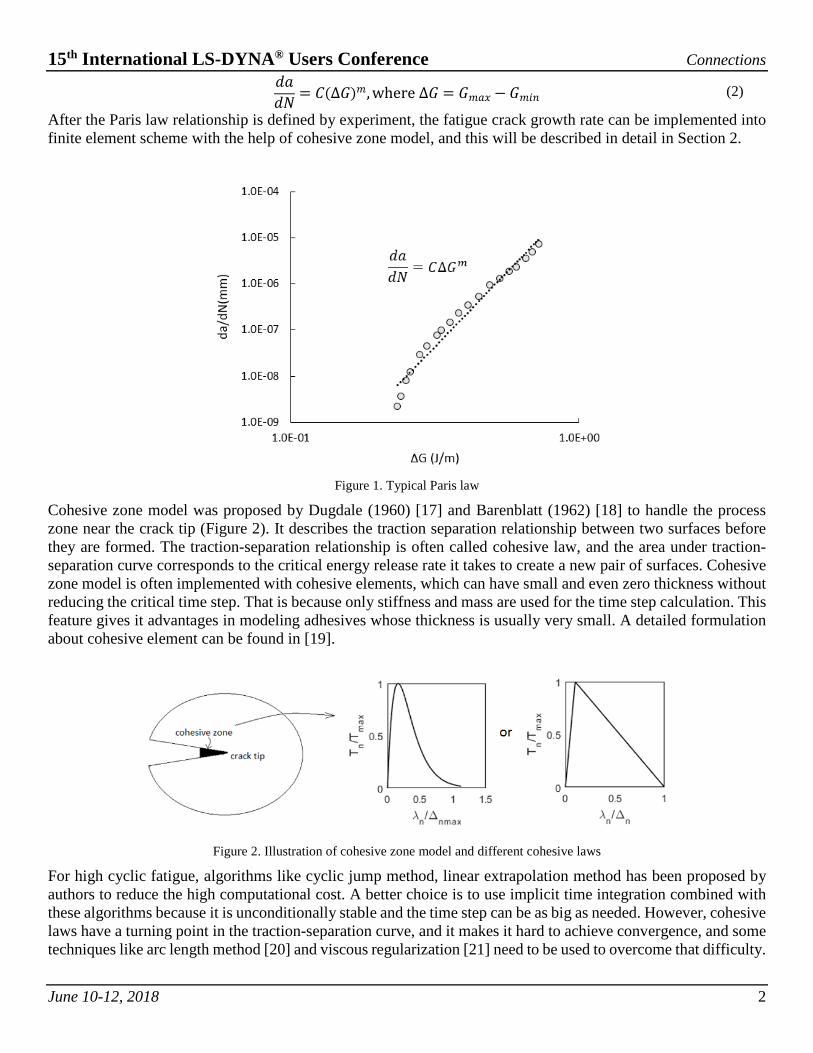
where 𝑑𝑑 is the crack length and 𝑑𝑑 is the number of loading cycles. D and B are curve fitting parameters of experiment data, and they can be considered as material parameters. Since correlation can be found between energy release rate and fracture toughness, Paris law can also be expressed in terms of energy release rate change (Equation 2), as shown in Figure 1.


June 10-12, 2018 2

𝑑𝑑𝑑𝑑𝑑𝑑𝑑𝑑 = 𝐶𝐶(∆𝐺𝐺)𝑚𝑚, where ∆𝐺𝐺 = 𝐺𝐺𝑚𝑚𝑑𝑑𝑚𝑚 − 𝐺𝐺𝑚𝑚𝑚𝑚𝑚𝑚 (2)

After the Paris law relationship is defined by experiment, the fatigue crack growth rate can be implemented into finite element scheme with the help of cohesive zone model, and this will be described in detail in Section 2.

Figure 1. Typical Paris law

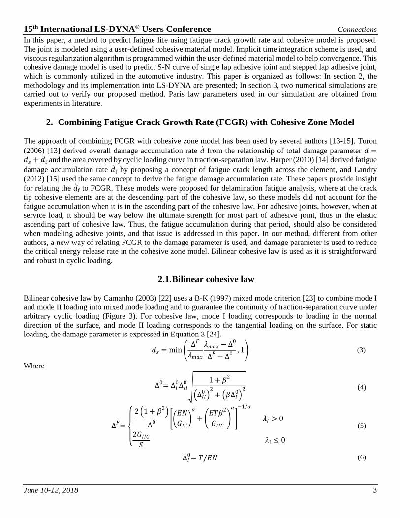
Cohesive zone model was proposed by Dugdale (1960) [17] and Barenblatt (1962) [18] to handle the process zone near the crack tip (Figure 2). It describes the traction separation relationship between two surfaces before they are formed. The traction-separation relationship is often called cohesive law, and the area under traction-separation curve corresponds to the critical energy release rate it takes to create a new pair of surfaces. Cohesive zone model is often implemented with cohesive elements, which can have small and even zero thickness without reducing the critical time step. That is because only stiffness and mass are used for the time step calculation. This feature gives it advantages in modeling adhesives whose thickness is usually very small. A detailed formulation about cohesive element can be found in [19].

Figure 2. Illustration of cohesive zone model and different cohesive laws

For high cyclic fatigue, algorithms like cyclic jump method, linear extrapolation method has been proposed by authors to reduce the high computational cost. A better choice is to use implicit time integration combined with these algorithms because it is unconditionally stable and the time step can be as big as needed. However, cohesive laws have a turning point in the traction-separation curve, and it makes it hard to achieve convergence, and some techniques like arc length method [20] and viscous regularization [21] need to be used to overcome that difficulty.


June 10-12, 2018 3

In this paper, a method to predict fatigue life using fatigue crack growth rate and cohesive model is proposed. The joint is modeled using a user-defined cohesive material model. Implicit time integration scheme is used, and viscous regularization algorithm is programmed within the user-defined material model to help convergence. This cohesive damage model is used to predict S-N curve of single lap adhesive joint and stepped lap adhesive joint, which is commonly utilized in the automotive industry. This paper is organized as follows: In section 2, the methodology and its implementation into LS-DYNA are presented; In section 3, two numerical simulations are carried out to verify our proposed method. Paris law parameters used in our simulation are obtained from experiments in literature.

2. Combining Fatigue Crack Growth Rate (FCGR) with Cohesive Zone Model The approach of combining FCGR with cohesive zone model has been used by several authors [13-15]. Turon (2006) [13] derived overall damage accumulation rate �̇�𝑑 from the relationship of total damage parameter 𝑑𝑑 =𝑑𝑑𝑠𝑠 + 𝑑𝑑f and the area covered by cyclic loading curve in traction-separation law. Harper (2010) [14] derived fatigue damage accumulation rate �̇�𝑑f by proposing a concept of fatigue crack length across the element, and Landry (2012) [15] used the same concept to derive the fatigue damage accumulation rate. These papers provide insight for relating the �̇�𝑑f to FCGR. These models were proposed for delamination fatigue analysis, where at the crack tip cohesive elements are at the descending part of the cohesive law, so these models did not account for the fatigue accumulation when it is in the ascending part of the cohesive law. For adhesive joints, however, when at service load, it should be way below the ultimate strength for most part of adhesive joint, thus in the elastic ascending part of cohesive law. Thus, the fatigue accumulation during that period, should also be considered when modeling adhesive joints, and that issue is addressed in this paper. In our method, different from other authors, a new way of relating FCGR to the damage parameter is used, and damage parameter is used to reduce the critical energy release rate in the cohesive zone model. Bilinear cohesive law is used as it is straightforward and robust in cyclic loading.

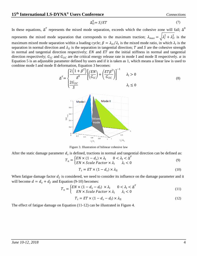
2.1. Bilinear cohesive law Bilinear cohesive law by Camanho (2003) [22] uses a B-K (1997) mixed mode criterion [23] to combine mode I and mode II loading into mixed mode loading and to guarantee the continuity of traction-separation curve under arbitrary cyclic loading (Figure 3). For cohesive law, mode I loading corresponds to loading in the normal direction of the surface, and mode II loading corresponds to the tangential loading on the surface. For static loading, the damage parameter is expressed in Equation 3 [24].

𝑑𝑑𝑠𝑠 = min �∆𝐹𝐹

𝜆𝜆𝑚𝑚𝑑𝑑𝑚𝑚𝜆𝜆𝑚𝑚𝑑𝑑𝑚𝑚 − ∆0

∆𝐹𝐹 − ∆0 , 1� (3)

Where

∆0= ∆𝐼𝐼0∆𝐼𝐼𝐼𝐼0 �1 + 𝛽𝛽2

�∆𝐼𝐼𝐼𝐼0 �2

+ �𝛽𝛽∆𝐼𝐼0�2 (4)

∆𝐹𝐹=

⎩⎪⎨

⎪⎧ 2 �1 + 𝛽𝛽2�

∆0 ��𝐸𝐸𝑑𝑑𝐺𝐺𝐼𝐼𝐶𝐶

�𝛼𝛼

+ �𝐸𝐸𝐸𝐸𝛽𝛽2

𝐺𝐺𝐼𝐼𝐼𝐼𝐶𝐶�𝛼𝛼

�

−1 𝛼𝛼⁄

𝜆𝜆𝐼𝐼 > 0

2𝐺𝐺𝐼𝐼𝐼𝐼𝐶𝐶𝑆𝑆 𝜆𝜆I ≤ 0

(5)

∆𝐼𝐼0= 𝐸𝐸/𝐸𝐸𝑑𝑑 (6)


June 10-12, 2018 4

∆𝐼𝐼𝐼𝐼0 = 𝑆𝑆/𝐸𝐸𝐸𝐸 (7)

In these equations, ∆𝐹𝐹 represents the mixed mode separation, exceeds which the cohesive zone will fail; ∆0

represents the mixed mode separation that corresponds to the maximum traction; 𝜆𝜆𝑚𝑚𝑑𝑑𝑚𝑚 = �𝜆𝜆𝐼𝐼2 + 𝜆𝜆𝐼𝐼𝐼𝐼

2 is the maximum mixed mode separation within a loading cycle; 𝛽𝛽 = 𝜆𝜆𝐼𝐼𝐼𝐼 𝜆𝜆𝐼𝐼⁄ is the mixed mode ratio, in which 𝜆𝜆𝐼𝐼 is the separation in normal direction and 𝜆𝜆𝐼𝐼𝐼𝐼 is the separation in tangential direction; 𝐸𝐸 and 𝑆𝑆 are the cohesive strength in normal and tangential direction respectively; 𝐸𝐸𝑑𝑑 and 𝐸𝐸𝐸𝐸 are the initial stiffness in normal and tangential direction respectively; 𝐺𝐺𝐼𝐼𝐶𝐶 and 𝐺𝐺𝐼𝐼𝐼𝐼𝐶𝐶 are the critical energy release rate in mode I and mode II respectively. 𝛼𝛼 in Equation 5 is an adjustable parameter defined by users and if it is taken as 1, which means a linear law is used to combine mode I and mode II deformation, Equation 3 becomes:

∆𝐹𝐹=

⎩⎪⎨

⎪⎧2 �1 + 𝛽𝛽2�

𝛿𝛿0 ��𝐸𝐸𝑑𝑑𝐺𝐺𝐼𝐼𝐶𝐶

�+ �𝐸𝐸𝐸𝐸𝛽𝛽2

𝐺𝐺𝐼𝐼𝐼𝐼𝐶𝐶��

−1

𝜆𝜆I > 0

2𝐺𝐺𝐼𝐼𝐼𝐼𝐶𝐶𝑆𝑆 𝜆𝜆I ≤ 0

(8)

Figure 3. Illustration of bilinear cohesive law

After the static damage parameter 𝑑𝑑𝑠𝑠 is defined, tractions in normal and tangential direction can be defined as:

𝐸𝐸𝑚𝑚 = �𝐸𝐸𝑑𝑑× (1− 𝑑𝑑𝑠𝑠) × 𝜆𝜆I 0 < 𝜆𝜆I < ∆𝐹𝐹𝐸𝐸𝑑𝑑× 𝑆𝑆𝑆𝑆𝑑𝑑𝑆𝑆𝑆𝑆 𝐹𝐹𝑑𝑑𝑆𝑆𝐹𝐹𝐹𝐹𝐹𝐹× 𝜆𝜆I 𝜆𝜆I < 0

(9)

𝐸𝐸𝐹𝐹 = 𝐸𝐸𝐸𝐸× (1− 𝑑𝑑𝑠𝑠) × 𝜆𝜆II (10)

When fatigue damage factor 𝑑𝑑𝑓𝑓 is considered, we need to consider its influence on the damage parameter and it will become 𝑑𝑑 = 𝑑𝑑𝑠𝑠 + 𝑑𝑑𝑓𝑓 and Equation (9-10) becomes:

𝐸𝐸𝑚𝑚 = �𝐸𝐸𝑑𝑑× (1− 𝑑𝑑𝑠𝑠 − 𝑑𝑑f) × 𝜆𝜆I 0 < 𝜆𝜆I < ∆𝐹𝐹𝐸𝐸𝑑𝑑× 𝑆𝑆𝑆𝑆𝑑𝑑𝑆𝑆𝑆𝑆 𝐹𝐹𝑑𝑑𝑆𝑆𝐹𝐹𝐹𝐹𝐹𝐹× 𝜆𝜆I 𝜆𝜆I < 0

(11)

𝐸𝐸𝐹𝐹 = 𝐸𝐸𝐸𝐸× (1− 𝑑𝑑𝑠𝑠 − 𝑑𝑑f) × 𝜆𝜆II (12)

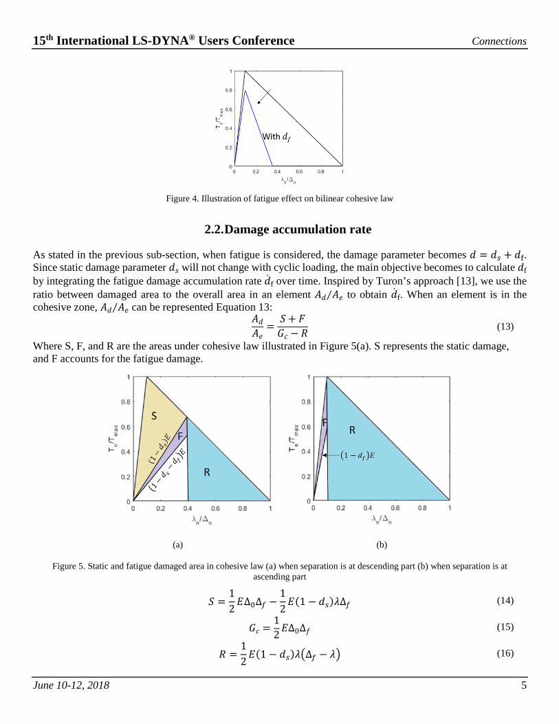
The effect of fatigue damage on Equation (11-12) can be illustrated in Figure 4.


June 10-12, 2018 5

Figure 4. Illustration of fatigue effect on bilinear cohesive law

2.2. Damage accumulation rate

As stated in the previous sub-section, when fatigue is considered, the damage parameter becomes 𝑑𝑑 = 𝑑𝑑𝑠𝑠 + 𝑑𝑑f. Since static damage parameter 𝑑𝑑𝑠𝑠 will not change with cyclic loading, the main objective becomes to calculate 𝑑𝑑f by integrating the fatigue damage accumulation rate �̇�𝑑f over time. Inspired by Turon’s approach [13], we use the ratio between damaged area to the overall area in an element 𝐴𝐴𝑑𝑑 𝐴𝐴𝑆𝑆⁄ to obtain �̇�𝑑f. When an element is in the cohesive zone, 𝐴𝐴𝑑𝑑 𝐴𝐴𝑆𝑆⁄ can be represented Equation 13:

𝐴𝐴𝑑𝑑𝐴𝐴𝑆𝑆

=𝑆𝑆+ 𝐹𝐹𝐺𝐺𝑆𝑆 − 𝑅𝑅 (13)

Where S, F, and R are the areas under cohesive law illustrated in Figure 5(a). S represents the static damage, and F accounts for the fatigue damage.

(a) (b)

Figure 5. Static and fatigue damaged area in cohesive law (a) when separation is at descending part (b) when separation is at ascending part

𝑆𝑆 =12𝐸𝐸∆0∆𝑓𝑓 −

12𝐸𝐸(1 − 𝑑𝑑𝑠𝑠)𝜆𝜆∆𝑓𝑓 (14)

𝐺𝐺𝑆𝑆 =12𝐸𝐸∆0∆𝑓𝑓 (15)

𝑅𝑅 =12𝐸𝐸(1 − 𝑑𝑑𝑠𝑠)𝜆𝜆�∆𝑓𝑓 − 𝜆𝜆� (16)


June 10-12, 2018 6

𝐹𝐹 =12𝐸𝐸(1 − 𝑑𝑑𝑠𝑠)𝜆𝜆2 −

12𝐸𝐸�1 − 𝑑𝑑𝑠𝑠 − 𝑑𝑑𝑓𝑓�𝜆𝜆2 (17)

In Equation (14-17), 𝐸𝐸 represents either 𝐸𝐸𝑑𝑑 or 𝐸𝐸𝐸𝐸, depending on whether it is normal or tangential loading. ∆𝑓𝑓 and ∆0 could also represent the characteristic separations in normal or tangential direction, in which ∆𝑓𝑓 is the maximum allowable separation and ∆0 is the separation at maximum traction. Plug Equation (14-17) back to Equation 13, we will get:


=∆0∆𝑓𝑓 − (1− 𝑑𝑑𝑠𝑠)𝜆𝜆∆𝑓𝑓 + (1− 𝑑𝑑𝑠𝑠)𝜆𝜆2 − �1− 𝑑𝑑𝑠𝑠 − 𝑑𝑑𝑓𝑓�𝜆𝜆

2

∆0∆𝑓𝑓 − (1− 𝑑𝑑𝑠𝑠)𝜆𝜆�∆𝑓𝑓 − 𝜆𝜆� (18)

where 𝜆𝜆 is the separation in mixed mode. By ignoring the influence of fatigue accumulation on static damage parameter, the damage accumulation rate can be expressed as:

𝜕𝜕𝑑𝑑𝜕𝜕𝑑𝑑 =

𝜕𝜕𝑑𝑑𝜕𝜕𝐴𝐴𝑑𝑑

𝜕𝜕𝐴𝐴𝑑𝑑𝜕𝜕𝑑𝑑 =

𝜕𝜕�𝑑𝑑𝑠𝑠 + 𝑑𝑑𝑓𝑓�𝜕𝜕𝐴𝐴𝑑𝑑


𝜕𝜕𝑑𝑑𝑓𝑓𝜕𝜕𝐴𝐴𝑑𝑑


𝜕𝜕𝑑𝑑𝑓𝑓𝜕𝜕𝑑𝑑 (19)

From Equation 18 we can get:


=1𝐴𝐴𝑆𝑆∆0∆𝑓𝑓 − (1− 𝑑𝑑𝑠𝑠)𝜆𝜆�∆𝑓𝑓 − 𝜆𝜆�

𝜆𝜆2 (20)

The increase of the damaged area along a crack front is equal to the sum of the damaged area increase of all the elements ahead of the crack tip. If the modeling of adhesive joint is using a constant element size, and since the damage at the crack front is approximately uniformly distributed through the width, we can assume that the damaged area of elements in cohesive zone is approximately the same, and the fatigue crack growth rate can be written as:

𝜕𝜕𝐴𝐴𝜕𝜕𝑑𝑑 =

𝐴𝐴𝑆𝑆𝑐𝑐𝐴𝐴𝑆𝑆

𝜕𝜕𝐴𝐴𝑑𝑑𝜕𝜕𝑑𝑑 (21)

where 𝐴𝐴𝑆𝑆𝑐𝑐 is the cohesive zone size. For mode I case [25]:

𝐴𝐴𝑆𝑆𝑐𝑐,𝐼𝐼 = 𝑏𝑏9𝜋𝜋32

𝐸𝐸𝐺𝐺𝐼𝐼𝐶𝐶𝐸𝐸2 (22)

Plug Equation (20-22) into Equation 19, we can get:

𝜕𝜕𝑑𝑑𝑓𝑓𝜕𝜕𝑑𝑑 =

32𝐸𝐸2

𝑏𝑏9𝜋𝜋𝐸𝐸𝐺𝐺𝐼𝐼𝐶𝐶 ∆0∆𝑓𝑓 − (1− 𝑑𝑑𝑠𝑠)𝜆𝜆𝐼𝐼�∆𝑓𝑓 − 𝜆𝜆𝐼𝐼�

𝜆𝜆𝐼𝐼2

𝜕𝜕𝐴𝐴𝜕𝜕𝑑𝑑 (23)

Assuming the adhesive joint has the same width across the section, it can be further simplified to:


32𝐸𝐸2

9𝜋𝜋𝐸𝐸𝐺𝐺𝐼𝐼𝐶𝐶 ∆0∆𝑓𝑓 − (1− 𝑑𝑑𝑠𝑠)𝜆𝜆𝐼𝐼�∆𝑓𝑓 − 𝜆𝜆𝐼𝐼�

𝜆𝜆𝐼𝐼2

𝜕𝜕𝑑𝑑𝜕𝜕𝑑𝑑 (24)

where 𝑑𝑑 is the crack length. Similarly, for mode II case the cohesive zone size can be approximated as: [26]

𝐴𝐴𝑆𝑆𝑐𝑐,𝐼𝐼𝐼𝐼 =𝑏𝑏𝐸𝐸𝐺𝐺𝐼𝐼𝐼𝐼𝐶𝐶𝑆𝑆2 (25)

In Mode II case the fatigue damage accumulation rate �̇�𝑑𝑓𝑓 would be:


𝑆𝑆2

𝐸𝐸𝐺𝐺𝐼𝐼𝐼𝐼𝐶𝐶 ∆0∆𝑓𝑓 − (1− 𝑑𝑑𝑠𝑠)𝜆𝜆𝐼𝐼𝐼𝐼�∆𝑓𝑓 − 𝜆𝜆𝐼𝐼𝐼𝐼�

𝜆𝜆𝐼𝐼𝐼𝐼2

𝜕𝜕𝑑𝑑𝜕𝜕𝑑𝑑 (26)

When it is at mixed mode loading case, linear interpolation is used to get the equivalent cohesive zone length:

𝐴𝐴𝑆𝑆𝑐𝑐 = 𝐴𝐴𝑆𝑆𝑐𝑐,𝐼𝐼 + 𝛽𝛽�𝐴𝐴𝑆𝑆𝑐𝑐,𝐼𝐼𝐼𝐼 − 𝐴𝐴𝑆𝑆𝑐𝑐,𝐼𝐼� (27)

where 𝛽𝛽 = 𝜆𝜆𝐼𝐼𝐼𝐼 𝜆𝜆𝐼𝐼⁄ is the mixed mode ratio. Then for mixed mode separation, �̇�𝑑𝑓𝑓 becomes:


𝑏𝑏𝐴𝐴𝑆𝑆𝑐𝑐

∆0∆𝑓𝑓 − (1− 𝑑𝑑𝑠𝑠)𝜆𝜆�∆𝑓𝑓 − 𝜆𝜆�

𝜆𝜆2𝜕𝜕𝑑𝑑𝜕𝜕𝑑𝑑 (28)

where 𝜆𝜆 is the mixed mode separation. Equation 24, 26 and 28 all represent the �̇�𝑑𝑓𝑓 expression when the separation is at the descending part of cohesive law.


June 10-12, 2018 7

For cases where separation is at the ascending part of cohesive zone (0 < 𝜆𝜆 < ∆0), like shown in Figure 5(b), a similar approach is used to obtain �̇�𝑑𝑓𝑓. We have 𝑑𝑑𝑠𝑠 = 0 and


=𝐹𝐹

𝐹𝐹+ 𝑅𝑅 =12𝐸𝐸𝜆𝜆

2 − 12𝐸𝐸�1− 𝑑𝑑𝑓𝑓�𝜆𝜆

2

12𝐸𝐸𝜆𝜆

2= 𝑑𝑑𝑓𝑓 (29)


=1𝐴𝐴𝑆𝑆

(30)

For mode I:


𝑏𝑏𝐴𝐴𝑆𝑆𝑐𝑐,𝐼𝐼


32𝐸𝐸2

9𝜋𝜋𝐸𝐸𝐺𝐺𝐼𝐼𝐶𝐶𝜕𝜕𝑑𝑑𝜕𝜕𝑑𝑑 (31)

For mode II:


𝑏𝑏𝐴𝐴𝑆𝑆𝑐𝑐,𝐼𝐼𝐼𝐼


𝑆𝑆2

𝐸𝐸𝐺𝐺𝐼𝐼𝐼𝐼𝐶𝐶𝜕𝜕𝑑𝑑𝜕𝜕𝑑𝑑 (32)

For mixed mode:


𝑏𝑏𝐴𝐴𝑆𝑆𝑐𝑐

𝜕𝜕𝑑𝑑𝜕𝜕𝑑𝑑 (33)

After the relationship between damage accumulation rate and fatigue crack growth rate is determined, we can relate it to the FCGR:

𝜕𝜕𝑑𝑑𝜕𝜕𝑑𝑑 = 𝐶𝐶(∆𝐺𝐺)𝑚𝑚 (34)

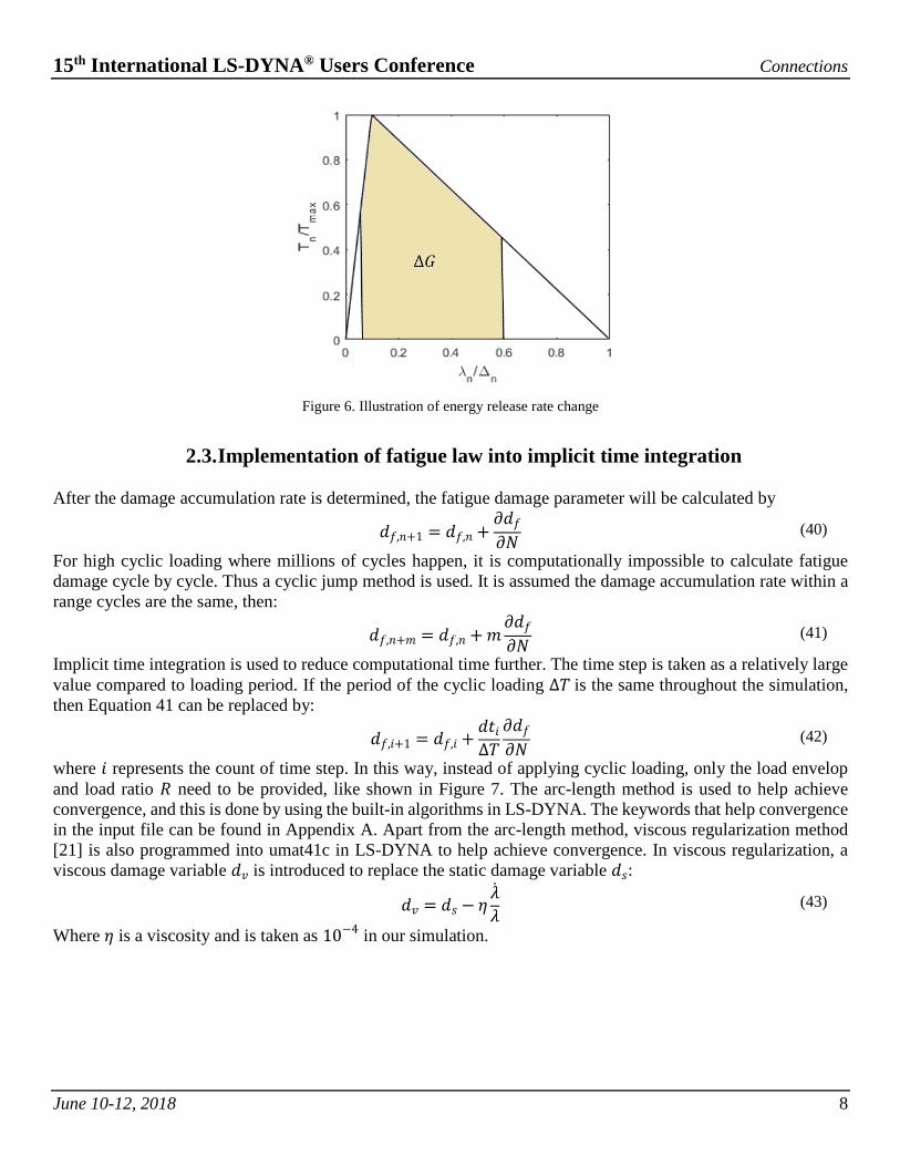
Parameters C and m for mode I and mode II can both be determined through experiment. The right-hand side of the equation is energy release rate change, which corresponds to the area under the traction separation law as shown in Figure 6. If the load ratio is known, the energy release rate can be calculated using Equation 35:

∆𝐺𝐺 =1

2𝐸𝐸(𝐸𝐸𝑚𝑚𝑚𝑚𝑚𝑚2 − 𝐸𝐸𝑚𝑚𝑚𝑚𝑚𝑚2 ) =

𝐸𝐸𝑚𝑚𝑚𝑚𝑚𝑚2

2𝐸𝐸(1 − 𝑅𝑅2) (35)

Regarding separation in normal and tangential direction, Equation 35 can be represented as:

∆𝐺𝐺𝑚𝑚 =𝐸𝐸𝜆𝜆𝑚𝑚2

2(1 − 𝑅𝑅2)(1− 𝑑𝑑𝑠𝑠)�1 − 𝑑𝑑𝑓𝑓� 𝑚𝑚 = 1,2 (36)

where 𝑚𝑚 = 1,2 represents mode I and mode II respectively. Mixed mode energy release rate change is obtained by linear interpolation of mode I and mode II.

∆𝐺𝐺 = ∆𝐺𝐺𝐼𝐼 + 𝛽𝛽(∆𝐺𝐺𝐼𝐼𝐼𝐼 − ∆𝐺𝐺𝐼𝐼) (37)

After that, linear interpolation is used to obtain the mixed mode FCGR parameters:

𝑆𝑆𝑚𝑚(𝐶𝐶) = 𝑆𝑆𝑚𝑚(𝐶𝐶𝐼𝐼𝐼𝐼) + [𝑆𝑆𝑚𝑚(𝐶𝐶𝐼𝐼) − 𝑆𝑆𝑚𝑚(𝐶𝐶𝐼𝐼𝐼𝐼)] �1 −𝐺𝐺𝐼𝐼𝐼𝐼𝐺𝐺𝑇𝑇� (38)

𝑚𝑚 = 𝑚𝑚𝐼𝐼 + (𝑚𝑚𝐼𝐼𝐼𝐼 − 𝑚𝑚𝐼𝐼) �𝐺𝐺𝐼𝐼𝐼𝐼𝐺𝐺𝑇𝑇� (39)

Where 𝐺𝐺𝐸𝐸 = 𝐺𝐺𝐼𝐼 + 𝐺𝐺𝐼𝐼𝐼𝐼.


June 10-12, 2018 8

Figure 6. Illustration of energy release rate change

2.3. Implementation of fatigue law into implicit time integration

After the damage accumulation rate is determined, the fatigue damage parameter will be calculated by

𝑑𝑑𝑓𝑓,𝑚𝑚+1 = 𝑑𝑑𝑓𝑓,𝑚𝑚 +𝜕𝜕𝑑𝑑𝑓𝑓𝜕𝜕𝑑𝑑 (40)

For high cyclic loading where millions of cycles happen, it is computationally impossible to calculate fatigue damage cycle by cycle. Thus a cyclic jump method is used. It is assumed the damage accumulation rate within a range cycles are the same, then:

𝑑𝑑𝑓𝑓,𝑚𝑚+𝑚𝑚 = 𝑑𝑑𝑓𝑓,𝑚𝑚 +𝑚𝑚𝜕𝜕𝑑𝑑𝑓𝑓𝜕𝜕𝑑𝑑 (41)

Implicit time integration is used to reduce computational time further. The time step is taken as a relatively large value compared to loading period. If the period of the cyclic loading ∆𝐸𝐸 is the same throughout the simulation, then Equation 41 can be replaced by:

𝑑𝑑𝑓𝑓,𝑚𝑚+1 = 𝑑𝑑𝑓𝑓,𝑚𝑚 +𝑑𝑑𝐹𝐹𝑚𝑚∆𝐸𝐸

𝜕𝜕𝑑𝑑𝑓𝑓𝜕𝜕𝑑𝑑 (42)

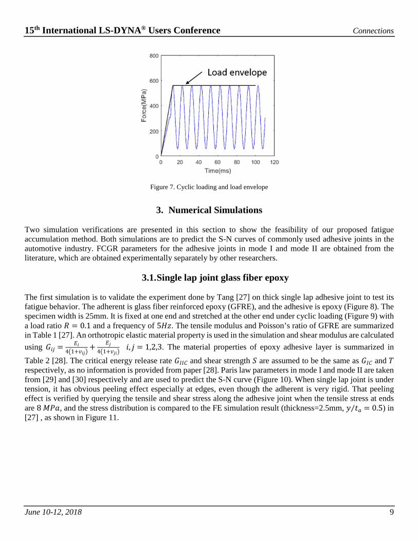
where 𝑚𝑚 represents the count of time step. In this way, instead of applying cyclic loading, only the load envelop and load ratio 𝑅𝑅 need to be provided, like shown in Figure 7. The arc-length method is used to help achieve convergence, and this is done by using the built-in algorithms in LS-DYNA. The keywords that help convergence in the input file can be found in Appendix A. Apart from the arc-length method, viscous regularization method [21] is also programmed into umat41c in LS-DYNA to help achieve convergence. In viscous regularization, a viscous damage variable 𝑑𝑑𝑣𝑣 is introduced to replace the static damage variable 𝑑𝑑𝑠𝑠:

𝑑𝑑𝑣𝑣 = 𝑑𝑑𝑠𝑠 − 𝜂𝜂�̇�𝜆𝜆𝜆 (43)

Where 𝜂𝜂 is a viscosity and is taken as 10−4 in our simulation.


June 10-12, 2018 9

Figure 7. Cyclic loading and load envelope

3. Numerical Simulations

Two simulation verifications are presented in this section to show the feasibility of our proposed fatigue accumulation method. Both simulations are to predict the S-N curves of commonly used adhesive joints in the automotive industry. FCGR parameters for the adhesive joints in mode I and mode II are obtained from the literature, which are obtained experimentally separately by other researchers.

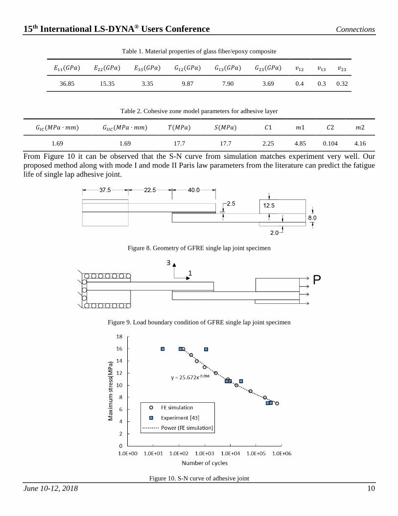
3.1. Single lap joint glass fiber epoxy The first simulation is to validate the experiment done by Tang [27] on thick single lap adhesive joint to test its fatigue behavior. The adherent is glass fiber reinforced epoxy (GFRE), and the adhesive is epoxy (Figure 8). The specimen width is 25mm. It is fixed at one end and stretched at the other end under cyclic loading (Figure 9) with a load ratio 𝑅𝑅 = 0.1 and a frequency of 5𝐻𝐻𝑐𝑐. The tensile modulus and Poisson’s ratio of GFRE are summarized in Table 1 [27]. An orthotropic elastic material property is used in the simulation and shear modulus are calculated using 𝐺𝐺𝑚𝑚𝑖𝑖 = 𝐸𝐸𝑚𝑚

4�1+𝑣𝑣𝑚𝑚𝑖𝑖�+ 𝐸𝐸𝑖𝑖

4�1+𝑣𝑣𝑖𝑖𝑚𝑚� 𝑚𝑚, 𝑖𝑖 = 1,2,3. The material properties of epoxy adhesive layer is summarized in

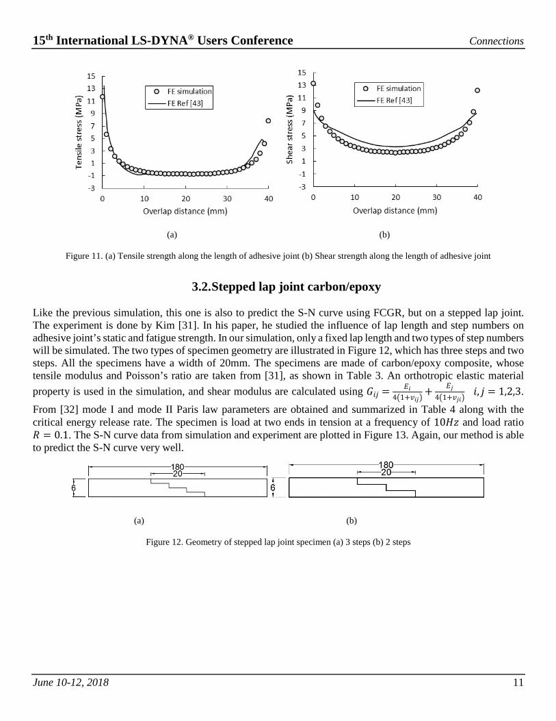
Table 2 [28]. The critical energy release rate 𝐺𝐺𝐼𝐼𝐼𝐼𝐶𝐶 and shear strength 𝑆𝑆 are assumed to be the same as 𝐺𝐺𝐼𝐼𝐶𝐶 and 𝐸𝐸 respectively, as no information is provided from paper [28]. Paris law parameters in mode I and mode II are taken from [29] and [30] respectively and are used to predict the S-N curve (Figure 10). When single lap joint is under tension, it has obvious peeling effect especially at edges, even though the adherent is very rigid. That peeling effect is verified by querying the tensile and shear stress along the adhesive joint when the tensile stress at ends are 8 𝑀𝑀𝑀𝑀𝑑𝑑, and the stress distribution is compared to the FE simulation result (thickness=2.5mm, 𝑦𝑦 𝐹𝐹𝑑𝑑⁄ = 0.5) in [27] , as shown in Figure 11.


June 10-12, 2018 10

Table 1. Material properties of glass fiber/epoxy composite

𝐸𝐸11(𝐺𝐺𝑀𝑀𝑑𝑑) 𝐸𝐸22(𝐺𝐺𝑀𝑀𝑑𝑑) 𝐸𝐸33(𝐺𝐺𝑀𝑀𝑑𝑑) 𝐺𝐺12(𝐺𝐺𝑀𝑀𝑑𝑑) 𝐺𝐺13(𝐺𝐺𝑀𝑀𝑑𝑑) 𝐺𝐺23(𝐺𝐺𝑀𝑀𝑑𝑑) 𝑣𝑣12 𝑣𝑣13 𝑣𝑣23

36.85 15.35 3.35 9.87 7.90 3.69 0.4 0.3 0.32

Table 2. Cohesive zone model parameters for adhesive layer

𝐺𝐺𝐼𝐼𝐼𝐼(𝑀𝑀𝑀𝑀𝑑𝑑 ∙ 𝑚𝑚𝑚𝑚) 𝐺𝐺𝐼𝐼𝐼𝐼𝐼𝐼(𝑀𝑀𝑀𝑀𝑑𝑑 ∙ 𝑚𝑚𝑚𝑚) 𝐸𝐸(𝑀𝑀𝑀𝑀𝑑𝑑) 𝑆𝑆(𝑀𝑀𝑀𝑀𝑑𝑑) 𝐶𝐶1 𝑚𝑚1 𝐶𝐶2 𝑚𝑚2

1.69 1.69 17.7 17.7 2.25 4.85 0.104 4.16

From Figure 10 it can be observed that the S-N curve from simulation matches experiment very well. Our proposed method along with mode I and mode II Paris law parameters from the literature can predict the fatigue life of single lap adhesive joint.

Figure 8. Geometry of GFRE single lap joint specimen

Figure 9. Load boundary condition of GFRE single lap joint specimen

Figure 10. S-N curve of adhesive joint


June 10-12, 2018 11

(a) (b)

Figure 11. (a) Tensile strength along the length of adhesive joint (b) Shear strength along the length of adhesive joint

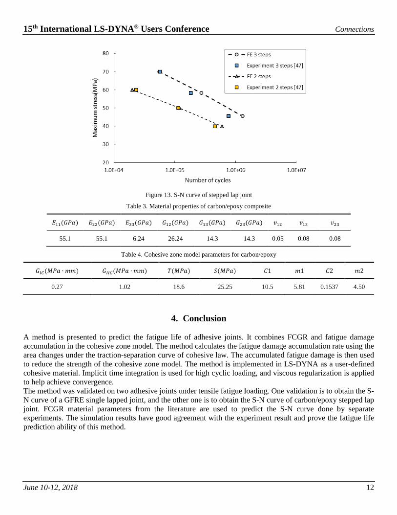
3.2. Stepped lap joint carbon/epoxy

Like the previous simulation, this one is also to predict the S-N curve using FCGR, but on a stepped lap joint. The experiment is done by Kim [31]. In his paper, he studied the influence of lap length and step numbers on adhesive joint’s static and fatigue strength. In our simulation, only a fixed lap length and two types of step numbers will be simulated. The two types of specimen geometry are illustrated in Figure 12, which has three steps and two steps. All the specimens have a width of 20mm. The specimens are made of carbon/epoxy composite, whose tensile modulus and Poisson’s ratio are taken from [31], as shown in Table 3. An orthotropic elastic material property is used in the simulation, and shear modulus are calculated using 𝐺𝐺𝑚𝑚𝑖𝑖 = 𝐸𝐸𝑚𝑚

4�1+𝑣𝑣𝑚𝑚𝑖𝑖�+ 𝐸𝐸𝑖𝑖

4�1+𝑣𝑣𝑖𝑖𝑚𝑚� 𝑚𝑚, 𝑖𝑖 = 1,2,3.

From [32] mode I and mode II Paris law parameters are obtained and summarized in Table 4 along with the critical energy release rate. The specimen is load at two ends in tension at a frequency of 10𝐻𝐻𝑐𝑐 and load ratio 𝑅𝑅 = 0.1. The S-N curve data from simulation and experiment are plotted in Figure 13. Again, our method is able to predict the S-N curve very well.

(a) (b)

Figure 12. Geometry of stepped lap joint specimen (a) 3 steps (b) 2 steps


June 10-12, 2018 12

Figure 13. S-N curve of stepped lap joint

Table 3. Material properties of carbon/epoxy composite

𝐸𝐸11(𝐺𝐺𝑀𝑀𝑑𝑑) 𝐸𝐸22(𝐺𝐺𝑀𝑀𝑑𝑑) 𝐸𝐸33(𝐺𝐺𝑀𝑀𝑑𝑑) 𝐺𝐺12(𝐺𝐺𝑀𝑀𝑑𝑑) 𝐺𝐺13(𝐺𝐺𝑀𝑀𝑑𝑑) 𝐺𝐺23(𝐺𝐺𝑀𝑀𝑑𝑑) 𝑣𝑣12 𝑣𝑣13 𝑣𝑣23

55.1 55.1 6.24 26.24 14.3 14.3 0.05 0.08 0.08

Table 4. Cohesive zone model parameters for carbon/epoxy

𝐺𝐺𝐼𝐼𝐼𝐼(𝑀𝑀𝑀𝑀𝑑𝑑 ∙ 𝑚𝑚𝑚𝑚) 𝐺𝐺𝐼𝐼𝐼𝐼𝐼𝐼(𝑀𝑀𝑀𝑀𝑑𝑑 ∙ 𝑚𝑚𝑚𝑚) 𝐸𝐸(𝑀𝑀𝑀𝑀𝑑𝑑) 𝑆𝑆(𝑀𝑀𝑀𝑀𝑑𝑑) 𝐶𝐶1 𝑚𝑚1 𝐶𝐶2 𝑚𝑚2

0.27 1.02 18.6 25.25 10.5 5.81 0.1537 4.50

4. Conclusion A method is presented to predict the fatigue life of adhesive joints. It combines FCGR and fatigue damage accumulation in the cohesive zone model. The method calculates the fatigue damage accumulation rate using the area changes under the traction-separation curve of cohesive law. The accumulated fatigue damage is then used to reduce the strength of the cohesive zone model. The method is implemented in LS-DYNA as a user-defined cohesive material. Implicit time integration is used for high cyclic loading, and viscous regularization is applied to help achieve convergence. The method was validated on two adhesive joints under tensile fatigue loading. One validation is to obtain the S-N curve of a GFRE single lapped joint, and the other one is to obtain the S-N curve of carbon/epoxy stepped lap joint. FCGR material parameters from the literature are used to predict the S-N curve done by separate experiments. The simulation results have good agreement with the experiment result and prove the fatigue life prediction ability of this method.


June 10-12, 2018 13

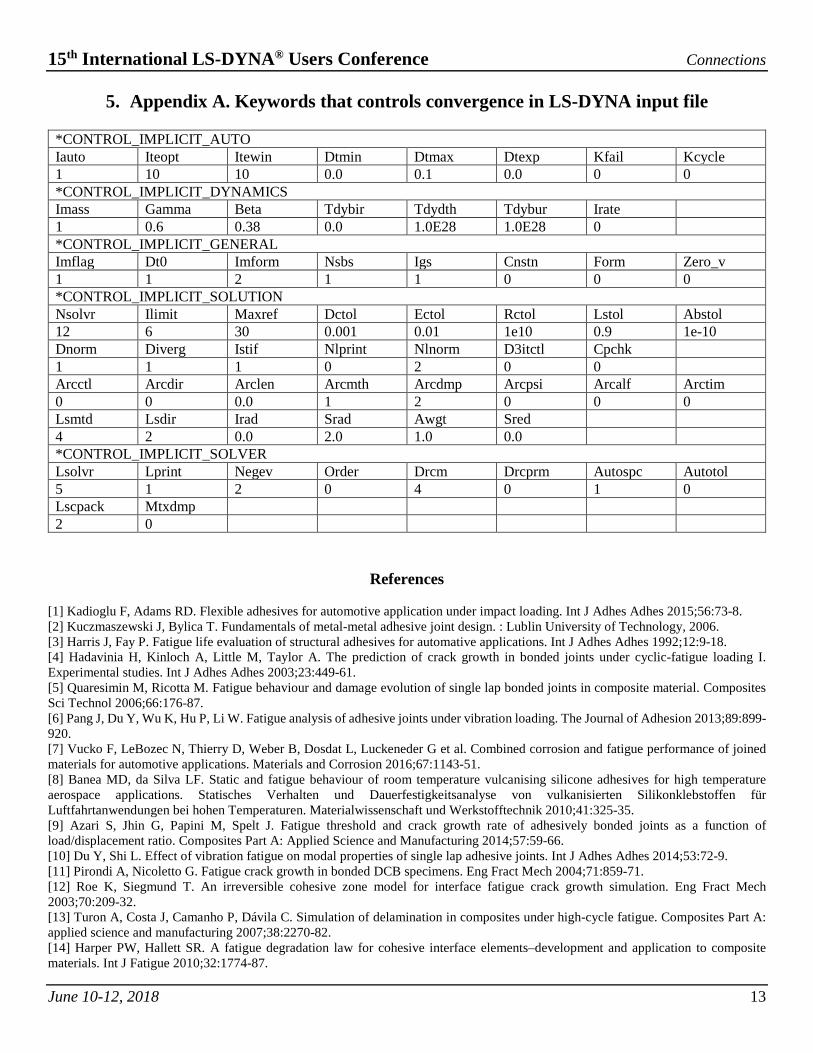
5. Appendix A. Keywords that controls convergence in LS-DYNA input file

*CONTROL_IMPLICIT_AUTO Iauto Iteopt Itewin Dtmin Dtmax Dtexp Kfail Kcycle 1 10 10 0.0 0.1 0.0 0 0 *CONTROL_IMPLICIT_DYNAMICS Imass Gamma Beta Tdybir Tdydth Tdybur Irate 1 0.6 0.38 0.0 1.0E28 1.0E28 0 *CONTROL_IMPLICIT_GENERAL Imflag Dt0 Imform Nsbs Igs Cnstn Form Zero_v 1 1 2 1 1 0 0 0 *CONTROL_IMPLICIT_SOLUTION Nsolvr Ilimit Maxref Dctol Ectol Rctol Lstol Abstol 12 6 30 0.001 0.01 1e10 0.9 1e-10 Dnorm Diverg Istif Nlprint Nlnorm D3itctl Cpchk 1 1 1 0 2 0 0 Arcctl Arcdir Arclen Arcmth Arcdmp Arcpsi Arcalf Arctim 0 0 0.0 1 2 0 0 0 Lsmtd Lsdir Irad Srad Awgt Sred 4 2 0.0 2.0 1.0 0.0 *CONTROL_IMPLICIT_SOLVER Lsolvr Lprint Negev Order Drcm Drcprm Autospc Autotol 5 1 2 0 4 0 1 0 Lscpack Mtxdmp 2 0

References [1] Kadioglu F, Adams RD. Flexible adhesives for automotive application under impact loading. Int J Adhes Adhes 2015;56:73-8. [2] Kuczmaszewski J, Bylica T. Fundamentals of metal-metal adhesive joint design. : Lublin University of Technology, 2006. [3] Harris J, Fay P. Fatigue life evaluation of structural adhesives for automative applications. Int J Adhes Adhes 1992;12:9-18. [4] Hadavinia H, Kinloch A, Little M, Taylor A. The prediction of crack growth in bonded joints under cyclic-fatigue loading I. Experimental studies. Int J Adhes Adhes 2003;23:449-61. [5] Quaresimin M, Ricotta M. Fatigue behaviour and damage evolution of single lap bonded joints in composite material. Composites Sci Technol 2006;66:176-87. [6] Pang J, Du Y, Wu K, Hu P, Li W. Fatigue analysis of adhesive joints under vibration loading. The Journal of Adhesion 2013;89:899-920. [7] Vucko F, LeBozec N, Thierry D, Weber B, Dosdat L, Luckeneder G et al. Combined corrosion and fatigue performance of joined materials for automotive applications. Materials and Corrosion 2016;67:1143-51. [8] Banea MD, da Silva LF. Static and fatigue behaviour of room temperature vulcanising silicone adhesives for high temperature aerospace applications. Statisches Verhalten und Dauerfestigkeitsanalyse von vulkanisierten Silikonklebstoffen für Luftfahrtanwendungen bei hohen Temperaturen. Materialwissenschaft und Werkstofftechnik 2010;41:325-35. [9] Azari S, Jhin G, Papini M, Spelt J. Fatigue threshold and crack growth rate of adhesively bonded joints as a function of load/displacement ratio. Composites Part A: Applied Science and Manufacturing 2014;57:59-66. [10] Du Y, Shi L. Effect of vibration fatigue on modal properties of single lap adhesive joints. Int J Adhes Adhes 2014;53:72-9. [11] Pirondi A, Nicoletto G. Fatigue crack growth in bonded DCB specimens. Eng Fract Mech 2004;71:859-71. [12] Roe K, Siegmund T. An irreversible cohesive zone model for interface fatigue crack growth simulation. Eng Fract Mech 2003;70:209-32. [13] Turon A, Costa J, Camanho P, Dávila C. Simulation of delamination in composites under high-cycle fatigue. Composites Part A: applied science and manufacturing 2007;38:2270-82. [14] Harper PW, Hallett SR. A fatigue degradation law for cohesive interface elements–development and application to composite materials. Int J Fatigue 2010;32:1774-87.


June 10-12, 2018 14

[15] Landry B, LaPlante G. Modeling delamination growth in composites under fatigue loadings of varying amplitudes. Composites Part B: Engineering 2012;43:533-41. [16] Pugno N, Ciavarella M, Cornetti P, Carpinteri A. A generalized Paris’ law for fatigue crack growth. J Mech Phys Solids 2006;54:1333-49. [17] Dugdale D. Yielding of steel sheets containing slits. J Mech Phys Solids 1960;8:100-4. [18] Barenblatt GI. The mathematical theory of equilibrium cracks in brittle fracture. Adv Appl Mech 1962;7:55-129. [19] Camanho PP, Dávila CG. Mixed-mode decohesion finite elements for the simulation of delamination in composite materials. 2002. [20] Crisfield M. An arc‐length method including line searches and accelerations. Int J Numer Methods Eng 1983;19:1269-89. [21] Yu H, Olsen JS, Olden V, Alvaro A, He J, Zhang Z. Viscous regularization for cohesive zone modeling under constant displacement: An application to hydrogen embrittlement simulation. Eng Fract Mech 2016;166:23-42. [22] Camanho PP, Davila C, De Moura M. Numerical simulation of mixed-mode progressive delamination in composite materials. J Composite Mater 2003;37:1415-38. [23] Benzeggagh M, Kenane M. Measurement of mixed-mode delamination fracture toughness of unidirectional glass/epoxy composites with mixed-mode bending apparatus. Composites Sci Technol 1996;56:439-49. [24] Livermore software technology corporation. LS-DYNA keyword user's manual volume II material models. In: Anonymous ; 2013. [25] Turon A, Camanho PP, Costa J, Dávila C. A damage model for the simulation of delamination in advanced composites under variable-mode loading. Mech Mater 2006;38:1072-89. [26] Harper PW, Hallett SR. Cohesive zone length in numerical simulations of composite delamination. Eng Fract Mech 2008;75:4774-92. [27] Tang J, Sridhar I, Srikanth N. Static and fatigue failure analysis of adhesively bonded thick composite single lap joints. Composites Sci Technol 2013;86:18-25. [28] Azari S, Papini M, Schroeder J, Spelt J. The effect of mode ratio and bond interface on the fatigue behavior of a highly-toughened epoxy. Eng Fract Mech 2010;77:395-414. [29] Brown EN, White SR, Sottos NR. Fatigue crack propagation in microcapsule-toughened epoxy. J Mater Sci 2006;41:6266-73. [30] O'Brien TK, Johnston WM, Toland GJ. Mode II interlaminar fracture toughness and fatigue characterization of a graphite epoxy composite material. 2010. [31] Kim J, Park B, Han Y. Evaluation of fatigue characteristics for adhesively-bonded composite stepped lap joint. Composite Structures 2004;66:69-75. [32] Asp LE, Sjögren A, Greenhalgh ES. Delamination growth and thresholds in a carbon/epoxy composite under fatigue loading. Journal of Composites, Technology and Research 2001;23:55-68.

Documents

Fatigue Life Prediction of Composite Adhesive Joints using