Embed Size (px)
Citation preview

USE IT OR LOSE IT:EFFICIENCY GAINS FROM WEALTH TAXATION
Fatih Guvenen Gueorgui Kambourov Burhan KuruscuMinnesota and NBER Toronto Toronto
Sergio Ocampo Daphne ChenMinnesota Econ One
January 17, 2017

The art of taxation consists in so plucking the goose...
...as to get the most feathers with the least hissing.
– Jean Baptiste Colbert, Minister of Finance to Louis XIV
Introduction Model Parameterization Tax Reform Optimal Taxation ROBUSTNESS Conclusions Extra
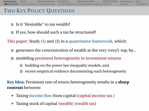
TWO KEY POLICY QUESTIONS
1 Is it “desirable” to tax wealth?
2 If yes, how should such a tax be structured?
This paper: Study (1) and (2) in a quantitative framework, which:
1 generates the concentration of wealth at the very (very!) top, by...
2 modeling persistent heterogeneity in investment returns
1 building on the power law inequality models, and
2 recent empirical evidence documenting such heterogeneity.
Key Idea: Persistent rate of return heterogeneity results in a sharpcontrast between:
œ Taxing income flow from capital (capital income tax )
œ Taxing stock of capital (wealth) (wealth tax)

Simple Example

Introduction Model Parameterization Tax Reform Optimal Taxation ROBUSTNESS Conclusions Extra
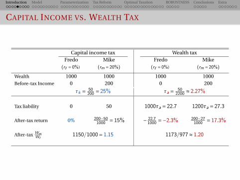
RETURN HETEROGENEITY: SIMPLE EXAMPLE
œ One-period model. Tax collected end of period.
œ Two brothers, Fredo and Mike, each with $1000 of wealth.
œ Key heterogeneity: in investment/entrepreneurial ability
(Fredo) Low ability: earns rf = 0% net return
(Mike) High ability: earns rm = 20% net return.
œ Government taxes to finance G = $50
Introduction Model Parameterization Tax Reform Optimal Taxation ROBUSTNESS Conclusions Extra
CAPITAL INCOME VS. WEALTH TAX
Capital income tax Wealth taxFredo Mike Fredo Mike
(rf = 0%) (rm = 20%) (rf = 0%) (rm = 20%)
Wealth 1000 1000 1000 1000Before-tax Income 0 200 0 200
øk = 50200 = 25% øa = 50
2200 º 2.27%
Tax liability 0 50 1000øa = 22.7 1200øa = 27.3
After-tax return 0% 200°501000 = 15% ° 22.7
1000 =°2.3% 200°271000 = 17.3%
After-tax WmWf
1150/1000= 1.15 1173/977º 1.20
Introduction Model Parameterization Tax Reform Optimal Taxation ROBUSTNESS Conclusions Extra
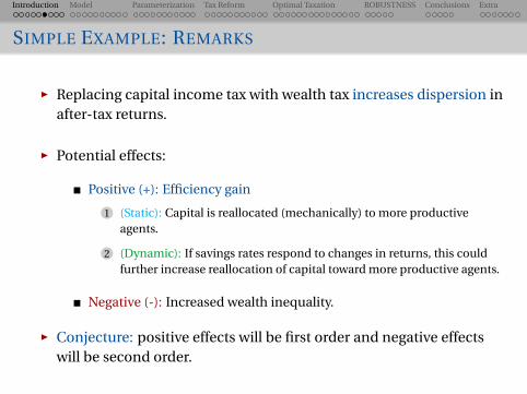
SIMPLE EXAMPLE: REMARKS
œ Replacing capital income tax with wealth tax increases dispersion inafter-tax returns.
œ Potential effects:
Positive (+): Efficiency gain
1 (Static): Capital is reallocated (mechanically) to more productiveagents.
2 (Dynamic): If savings rates respond to changes in returns, this couldfurther increase reallocation of capital toward more productive agents.
Negative (-): Increased wealth inequality.
œ Conjecture: positive effects will be first order and negative effectswill be second order.

Introduction Model Parameterization Tax Reform Optimal Taxation ROBUSTNESS Conclusions Extra
WHY MISALLOCATION IN THE LONG RUN?
œ In this simple example, we assumed that Mike and Fredo had thesame initial wealth.
œ But if this static example is repeated over and over, Mike willeventually hold all the aggregate wealth.
œ If so, maybe the misallocation of wealth to unproductive individualswill be a small problem?

Introduction Model Parameterization Tax Reform Optimal Taxation ROBUSTNESS Conclusions Extra
SOURCES OF MISALLOCATION: VARIATION IN RETURNS
œ Across Generations
Children of very successful entrepreneurs often inherit largeamounts of wealth but may not be able to work it efficiently.
œ Over the Life Cycle
One-hit wonders versus serial entrepreneurs.
Sector-specific shocks.
œ Wealth tax:
alleviates misallocation of capital across entrepreneurs with differentproductivities.
is like pruning: eliminates weak branches, strengthens stronger ones.

Introduction Model Parameterization Tax Reform Optimal Taxation ROBUSTNESS Conclusions Extra
OUTLINE
1 Model
2 Parameterization
3 Tax reform experiment
4 Optimal taxation
5 Robustness
6 Conclusions and current work
MODEL

Introduction Model Parameterization Tax Reform Optimal Taxation ROBUSTNESS Conclusions Extra
HOW DID RICH BECOME RICH?
FIGURE: Precautionary Saving or Higher Returns?

Introduction Model Parameterization Tax Reform Optimal Taxation ROBUSTNESS Conclusions Extra
NEW MODELS OF INEQUALITY
œ First generation models: rely on idiosyncratic income risk andprecautionary savings to generate wealth inequality. BUT:
Empirically measured income risk cannot generate much wealthconcentration at top end (Guvenen, Karahan, Ozkan, Song (2015)).No Pareto tail.
œ New literature: builds power law models of inequality (Benhabib,Bisin, et al (2011–2016), Gabaix, Lasry, Lions, and Moll (2016))
Persistent heterogeneity in returns is key for generating Pareto tailand concentration at top.
œ Fagereng, Guiso, Malacrino, and Pistaferri (2015) document largeheterogeneity and permanent differences in rate of returns(adjusted for risk).

Introduction Model Parameterization Tax Reform Optimal Taxation ROBUSTNESS Conclusions Extra
HOUSEHOLDS
œ OLG demographic structure.
œ Individuals face mortality risk and can live up to H years.
œ Let ¡h be the unconditional probability of survival up to age h,where ¡1 = 1.
œ Each household supplies labor in the market and produces adifferentiated intermediate good using her capital (wealth) andborrowing from the credit market.
œ Households maximize E0°PH
h=1Øh°1¡hu(ch,`h)
¢
œ Accidental bequests are inherited by (newborn) offspring.

Introduction Model Parameterization Tax Reform Optimal Taxation ROBUSTNESS Conclusions Extra
HOUSEHOLD LABOR MARKET EFFICIENCY
œ Labor market efficiency of household i at age h is
logyih = ∑h|{z}life cycle
+ µi|{z}permanent
+ ¥ih|{z}AR(1)
œ Individual-specific labor market efficiency µi is imperfectlyinherited from parents:
µchildi = Ωµµparenti +"µ
Introduction Model Parameterization Tax Reform Optimal Taxation ROBUSTNESS Conclusions Extra
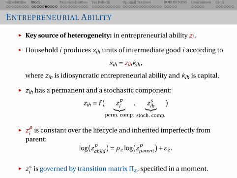
ENTREPRENEURIAL ABILITY
œ Key source of heterogeneity: in entrepreneurial ability zi .
œ Household i produces xih units of intermediate good i according to
xih = zihkih,
where zih is idiosyncratic entrepreneurial ability and kih is capital.
œ zih has a permanent and a stochastic component:
zih = f ( zpi|{z}perm. comp.
, zsih|{z}stoch. comp.
)
œ zpi is constant over the lifecycle and inherited imperfectly fromparent:
log(zpchild
)= Ωz log(zpparent)+"z .
œ zsi is governed by transition matrix¶z , specified in a moment.

Introduction Model Parameterization Tax Reform Optimal Taxation ROBUSTNESS Conclusions Extra
COMPETITIVE FINAL GOOD PRODUCER
œ Final good output is Y =QÆL1°Æ, where
Q =µZ
ixµi di
∂1/µ, µ< 1.
œ Price of intermediate good i is
pi (xi )=Æxµ°1i £QÆ°µL1°Æ.
œ Wage rate (per efficiency unit of labor) is
w = (1°Æ)QÆL°Æ.

Introduction Model Parameterization Tax Reform Optimal Taxation ROBUSTNESS Conclusions Extra
HOUSEHOLD BUDGET
œ Households can borrow up to a limit to finance their production:k ∑#(z)£a
Setting #(z)= 1) HH’s cannot borrow or lend.
Borrowing capacity is nondecreasing in ability: d#(z)/dz ∏ 0
œ Households can lend at interest rate r , determined in equilibrium(zero net supply).
œ Letting p =ÆQÆ°µL1°Æ, without taxes, wealth after-production:
max
k∑#(z)a[(1°±)k +p£ (zk)µ° (1+ r)(k °a)]
= (1+ r)a+º§(a,z)
œ After-tax wealth:
¶(a,z ;øk)=a+ [ra+º§(a,z)](1°øk) under capital income tax
¶(a,z ;øa)= [(1+ r)a+º§(a,z)](1°øa) under wealth tax

Introduction Model Parameterization Tax Reform Optimal Taxation ROBUSTNESS Conclusions Extra
HOUSEHOLD BUDGET
œ During retirement:
(1+øc)c +a0 =¶(a,z ;ø)+yR(µ,¥)
œ During working life:
(1+øc)c +a0 =¶(a,z ;ø)+ (1°ø`)(wyhn)√
and a0 ∏ 0 at all ages.
œ Benchmark: √¥ 1 (flat labor income tax)
œ Without heterogeneity in z and with µ= 1, the two tax systems areequivalent.
Introduction Model Parameterization Tax Reform Optimal Taxation ROBUSTNESS Conclusions Extra
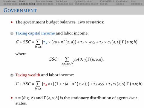
GOVERNMENT
œ The government budget balances. Two scenarios:
1 Taxing capital income and labor income:
G +SSC =X
h,a,s[øk £ (ra+º§
(z ,a))+ø`£wyh+øc £ch(a,s)]°(a,s;h)
whereSSC =
X
a,s,h∏RyR(µ,¥)G(h,a,s).
2 Taxing wealth and labor income:
G +SSC =X
h,a,s[øa£ (((1+ r)a+º§
(z ,a)))+ø`wyh+øcch(a,s)]°(a,s;h)
œ s¥ (µ,¥,z) and °(a,s;h) is the stationary distribution of agents overstates.

Introduction Model Parameterization Tax Reform Optimal Taxation ROBUSTNESS Conclusions Extra
FUNCTIONAL FORMS AND PARAMETERS
œ Preferences:
u(c ,`)=(c∞`1°∞
)
1°æ
1°æ
œ Pension system:
yR(µ,¥)=©(µ,¥)£Y where Y is the average labor income ineconomy, and
©(µ,¥) is a concave replacement rate function taken from SocialSecurity’s OASDI system.

Introduction Model Parameterization Tax Reform Optimal Taxation ROBUSTNESS Conclusions Extra
ENTREPRENEURIAL ABILITY: STOCHASTIC COMPONENT
œ The lifecycle pattern of wealth accumulation for the very richmatters greatly for the effects of wealth taxation:
1 steady accumulation of wealth: the rich today have high expectedreturns tomorrow.
œ Distortion is smaller. But wealthy are also more in favor ofwealth taxation.
2 extremely fast growth followed by stagnation: rich today have lowexpected returns tomorrow.
œ Distortion is big. Wealthy are not supportive of wealth taxes.
œ With fixed productivity, zp , returns fall as wealth increases (sinceµ< 1), but not sufficiently.
œ So, we consider a process that allows for both scenarios.
Introduction Model Parameterization Tax Reform Optimal Taxation ROBUSTNESS Conclusions Extra
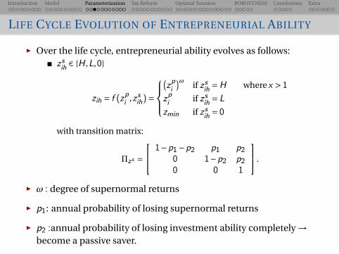
LIFE CYCLE EVOLUTION OF ENTREPRENEURIAL ABILITY
œ Over the life cycle, entrepreneurial ability evolves as follows:zsih 2 {H ,L,0}
zih = f (zpi ,zsih)=
8><
>:
°zpi
¢! if zsih =H wherex > 1zpi if zsih = L
zmin if zsih = 0
with transition matrix:
¶zs =
2
41°p1°p2 p1 p2
0 1°p2 p20 0 1
3
5 .
œ ! : degree of supernormal returns
œ p1: annual probability of losing supernormal returns
œ p2 :annual probability of losing investment ability completely !become a passive saver.

Introduction Model Parameterization Tax Reform Optimal Taxation ROBUSTNESS Conclusions Extra
TWO CALIBRATION TARGETS
œ Baseline:1 match the fraction of Forbes 400 rich that are self-made (54%, we get
50%)2 match the life cycle pattern of wealth accumulation for Forbes 400
(still in progress) FORBES 400 - (CIVALE AND DÍEZ-CATALÁN (2016))
œ Permanent z alone does not create enough self-made Forbes 400rich.
It takes too long (2-3 generations) to get into Forbes 400.
œ We choose: != 5, p1 = 0.05, and p2 = 0.03.
œ We also have robustness analysis with constant productivity: != 1,p1 = 0, and p2 = 0.
Introduction Model Parameterization Tax Reform Optimal Taxation ROBUSTNESS Conclusions Extra
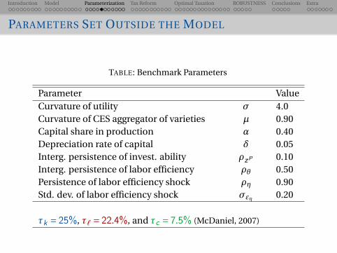
PARAMETERS SET OUTSIDE THE MODEL
TABLE: Benchmark Parameters
Parameter ValueCurvature of utility æ 4.0Curvature of CES aggregator of varieties µ 0.90Capital share in production Æ 0.40Depreciation rate of capital ± 0.05Interg. persistence of invest. ability ΩzP 0.10Interg. persistence of labor efficiency Ωµ 0.50Persistence of labor efficiency shock Ω¥ 0.90Std. dev. of labor efficiency shock æ"¥ 0.20
øk = 25%, ø` = 22.4%, and øc = 7.5% (McDaniel, 2007)

Introduction Model Parameterization Tax Reform Optimal Taxation ROBUSTNESS Conclusions Extra
CALIBRATION TARGETS AND OUTCOMES
œ ΩzP = 0.1 is set based on Fagereng et al (2016) for Norway. (We havealso experimented with values up to 0.5)
œ We calibrate 4 remaining parameters (Ø,∞,æ"zp ,æ"µ) to match 4data moments:
TABLE: Benchmark Parameters Calibrated Jointly in Equilibrium
Parameter Value MomentDiscount factor Ø 00.948 Capital/Output 3.00§
Cons. share in U ∞ 0.46 Avg. Hours 0.40§
æ of entrepr. ability æ"zp 0.072 Top 1% share 0.36§
æ of labor fix. eff. æ"µ 0.305 æ(log(Earn)) 0.80§

Introduction Model Parameterization Tax Reform Optimal Taxation ROBUSTNESS Conclusions Extra
MOMENTS
TABLE: Benchmark vs. Wealth Tax Economy
US Data Benchmark Wealth TaxTop 1% 0.36§ 0.36
Capital/Output 3.00§ 3.00Bequest/Wealth 1–2%00 0 0.99%
æ(log(Earnings)) 0.80§ 0.80Avg. Hours 0.40§ 0.40
œ Calibrated model generates:
total tax revenues: 25% of GDP (29.5% in the data)ratio of capital tax revenue to total tax revenue: 25% (28% in the data)
Introduction Model Parameterization Tax Reform Optimal Taxation ROBUSTNESS Conclusions Extra
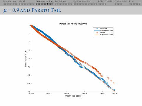
µ= 0.9 AND PARETO TAIL
1e+06 1e+07 1e+08 1e+09 1e+10 5e+10
Wealth (log scale)
-16
-14
-12
-10
-8
-6
-4
-2
0L
og
Co
un
ter-
CD
FPareto Tail Above $1000000
US DataRegression LineModelRegression Line
Quantitative Results
Introduction Model Parameterization Tax Reform Optimal Taxation ROBUSTNESS Conclusions Extra
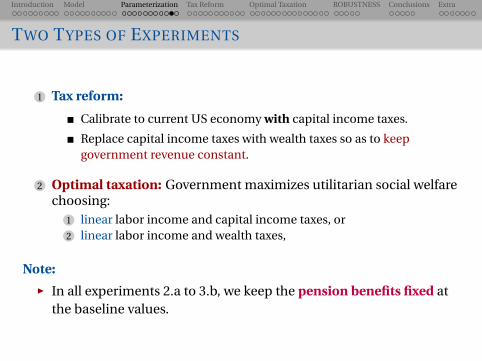
TWO TYPES OF EXPERIMENTS
1 Tax reform:
Calibrate to current US economy with capital income taxes.
Replace capital income taxes with wealth taxes so as to keepgovernment revenue constant.
2 Optimal taxation: Government maximizes utilitarian social welfarechoosing:
1 linear labor income and capital income taxes, or2 linear labor income and wealth taxes,
Note:
œ In all experiments 2.a to 3.b, we keep the pension benefits fixed atthe baseline values.

Introduction Model Parameterization Tax Reform Optimal Taxation ROBUSTNESS Conclusions Extra
PREVIEW OF EXTENSIONS WE HAVE STUDIED
1 Progressive labor income taxes (Reform & Optimal)
2 Progressive wealth taxes–flat tax, single threshold (Optimal)
3 No financial constraints (Reform & Optimal)
4 Unlimited borrowing, with Rborrow ¿Rsave (Optimal)
5 Log utility (Reform and Optimal)
6 zih = zpi at all ages (Reform and Optimal)
7 µ= 0.8 (Reform, Optimal—in progress)
8 Estate taxes, calibrated (Reform and Optimal, both in progress)
9 Consumption taxes (Optimal—in progress).
10 Some more extensions...
Summary: The substantive conclusions presented next are robust toALL these extensions.
1. Tax Reform

Introduction Model Parameterization Tax Reform Optimal Taxation ROBUSTNESS Conclusions Extra
RATE OF RETURN HETEROGENEITY
TABLE: Benchmark vs. Wealth Tax Economy
Percentiles of Return Distribution (%)
P10 P50 P90 P95 P99
Before-tax
Benchmark 2.00 2.00 17.28 22.35 42.36
Wealth tax 1.74 1.74 14.62 19.04 36.91
After-tax
Benchmark 1.50 1.50 12.96 16.76 31.77
Wealth tax 0.59 0.59 13.32 17.69 35.35
Introduction Model Parameterization Tax Reform Optimal Taxation ROBUSTNESS Conclusions Extra
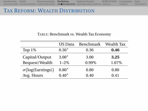
TAX REFORM: WEALTH DISTRIBUTION
TABLE: Benchmark vs. Wealth Tax Economy
US Data Benchmark Wealth TaxTop 1% 0.36§ 0.36 0.46
Capital/Output 3.00§ 3.00 3.25Bequest/Wealth 1–2%00 00.99% 01.07%
æ(log(Earnings)) 0.80§ 0.80 0.80Avg. Hours 0.40§ 0.40 0.41
Introduction Model Parameterization Tax Reform Optimal Taxation ROBUSTNESS Conclusions Extra
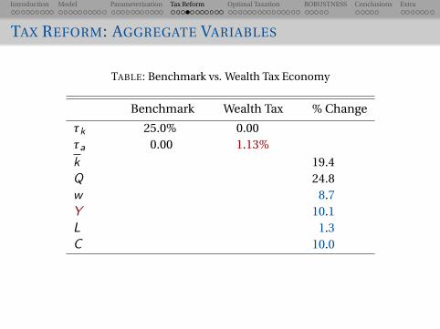
TAX REFORM: AGGREGATE VARIABLES
TABLE: Benchmark vs. Wealth Tax Economy
Benchmark Wealth Tax % Change
øk 0025.0% 000.00øa 0.00 1.13%k 19.4Q 24.8w 8.7Y 10.1L 1.3C 10.0
Introduction Model Parameterization Tax Reform Optimal Taxation ROBUSTNESS Conclusions Extra
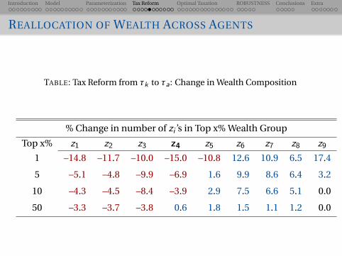
REALLOCATION OF WEALTH ACROSS AGENTS
TABLE: Tax Reform from øk to øa: Change in Wealth Composition
% Change in number of zi ’s in Top x% Wealth Group
Top x% z1 z2 z3 z4 z5 z6 z7 z8 z9
1 –14.8 –11.7 –10.0 –15.0 –10.8 12.6 10.9 6.5 17.4
5 –5.1 –4.8 –9.9 –6.9 1.6 9.9 8.6 6.4 3.2
10 –4.3 –4.5 –8.4 –3.9 2.9 7.5 6.6 5.1 0.0
50 –3.3 –3.7 –3.8 0.6 1.8 1.5 1.1 1.2 0.0

Introduction Model Parameterization Tax Reform Optimal Taxation ROBUSTNESS Conclusions Extra
WELFARE ANALYSIS: TWO MEASURES
Let s0 ¥ (µ,z ,a0), and V0 and V0 be lifetime value function in benchmark(US) and counterfactual economies, respectively.
œ Measure 1: Compute individual specific consumption equivalentwelfare and integrate:
V0((1+CE1(s0))c§US(s0),`§US(s0))=V0(c(s0),`(s0))
CE 1 ¥X
s0°US(s0)£CE (s0)
œ Measure 2: Fixed proportional consumption transfer to allindividuals in the benchmark economy:
X
s0°US(s0)£V0((1+CE 2)c
§US(s0),`§US(s0))=
X
s0°(s0)£V0(c(s0),`(s0)).

Introduction Model Parameterization Tax Reform Optimal Taxation ROBUSTNESS Conclusions Extra
TAX REFORM: WHO GAINS, WHO LOSES?
Productivity group
Age z1 z2 z3 z4 z5 z6 z7 z8 z9
20–25 7.3 7.2 6.8 6.8 7.4 8.8 10.5 11.1 10.7
25–34 7.0 6.9 6.4 6.0 5.9 6.0 5.9 3.7 1.2
35–44 6.1 6.0 5.4 4.9 4.3 3.3 1.4 -1.7 -4.3
45–54 4.6 4.5 4.1 3.5 2.8 1.7 -0.5 -3.1 -5.2
55–64 1.9 1.9 1.6 1.3 0.9 0.0 -1.6 -3.5 -5.3
65–74 -0.3 -0.3 -0.4 -0.5 -0.6 -1.0 -2.1 -3.4 -4.7
75+ -0.1 -0.1 -0.1 -0.1 -0.1 -0.4 -1.0 -1.9 -2.7
Note: Each cell reports the average of CE1(µ,z ,a,h)£100 within each age andproductivity group

Introduction Model Parameterization Tax Reform Optimal Taxation ROBUSTNESS Conclusions Extra
SHARING THE GAINS WITH RETIREES
Productivity group
Age z1 z2 z3 z4 z5 z6 z7 z8 z9
20–25 5.3 5.2 4.8 4.9 5.7 7.4 9.6 10.6 10.4
25–34 5.3 5.1 4.6 4.4 4.5 5.0 5.2 3.2 0.6
35–44 4.9 4.8 4.3 3.8 3.4 2.8 0.9 -2.4 -5.3
45–54 4.8 4.7 4.3 3.8 3.3 2.1 -0.2 -3.1 -5.6
55–64 5.6 5.6 5.3 4.8 4.3 3.1 0.8 -1.9 -4.3
65–74 7.0 7.0 6.8 6.3 5.8 4.7 2.6 0.1 –2.2
75+ 7.7 7.7 7.6 7.4 7.0 6.2 4.5 2.5 0.6
Note: Each cell reports the average of CE1(µ,z ,a,h)£100 within each age andproductivity group

Introduction Model Parameterization Tax Reform Optimal Taxation ROBUSTNESS Conclusions Extra
POLITICAL SUPPORT FOR WEALTH TAXES
Productivity group
Age z1 z2 z3 z4 z5 z6 z7 z8 z9
20–25 0.98 0.98 0.96 0.96 0.97 0.97 0.97 0.97 0.94
25–34 0.99 0.99 0.98 0.97 0.95 0.94 0.89 0.78 0.59
35–44 0.98 0.98 0.97 0.95 0.91 0.84 0.67 0.45 0.34
45–54 0.96 0.96 0.93 0.90 0.84 0.71 0.54 0.41 0.31
55–64 0.77 0.77 0.73 0.70 0.64 0.53 0.42 0.32 0.24
65–74 0.00 0.06 0.06 0.08 0.09 0.08 0.06 0.04 0.03
75+ 0.00 0.12 0.09 0.11 0.10 0.09 0.07 0.05 0.04
Introduction Model Parameterization Tax Reform Optimal Taxation ROBUSTNESS Conclusions Extra
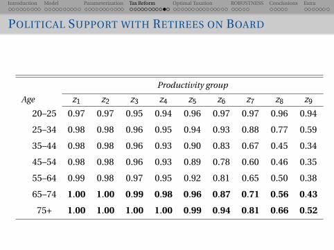
POLITICAL SUPPORT WITH RETIREES ON BOARD
Productivity group
Age z1 z2 z3 z4 z5 z6 z7 z8 z9
20–25 0.97 0.97 0.95 0.94 0.96 0.97 0.97 0.96 0.94
25–34 0.98 0.98 0.96 0.95 0.94 0.93 0.88 0.77 0.59
35–44 0.98 0.98 0.96 0.93 0.90 0.83 0.67 0.45 0.34
45–54 0.98 0.98 0.96 0.93 0.89 0.78 0.60 0.46 0.35
55–64 0.99 0.98 0.97 0.95 0.92 0.81 0.65 0.50 0.38
65–74 1.00 1.00 0.99 0.98 0.96 0.87 0.71 0.56 0.43
75+ 1.00 1.00 1.00 1.00 0.99 0.94 0.81 0.66 0.52
Introduction Model Parameterization Tax Reform Optimal Taxation ROBUSTNESS Conclusions Extra
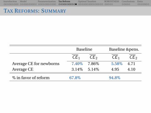
TAX REFORMS: SUMMARY
Baseline Baseline &pens.
CE 1 CE 2 CE 1 CE 2
Average CE for newborns 7.40% 7.86% 5.58% 4.71Average CE 3.14% 5.14% 4.95 4.10
% in favor of reform 67.8% 94.8%

Optimal Taxation
Introduction Model Parameterization Tax Reform Optimal Taxation ROBUSTNESS Conclusions Extra
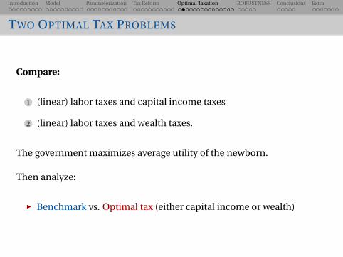
TWO OPTIMAL TAX PROBLEMS
Compare:
1 (linear) labor taxes and capital income taxes
2 (linear) labor taxes and wealth taxes.
The government maximizes average utility of the newborn.
Then analyze:
œ Benchmark vs. Optimal tax (either capital income or wealth)
Introduction Model Parameterization Tax Reform Optimal Taxation ROBUSTNESS Conclusions Extra
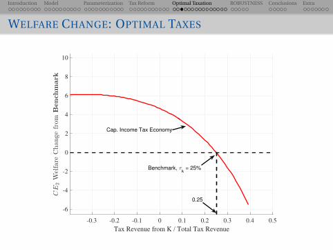
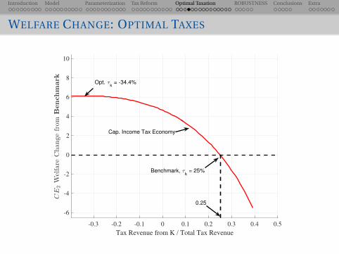
WELFARE CHANGE: OPTIMAL TAXES
-0.3 -0.2 -0.1 0 0.1 0.2 0.3 0.4 0.5
Tax Revenue from K / Total Tax Revenue
-6
-4
-2
0
2
4
6
8
10CE
2Welfare
Changefrom
Benchmark
Cap. Income Tax Economy
Benchmark, τk = 25%
0.25
Introduction Model Parameterization Tax Reform Optimal Taxation ROBUSTNESS Conclusions Extra
WELFARE CHANGE: OPTIMAL TAXES
-0.3 -0.2 -0.1 0 0.1 0.2 0.3 0.4 0.5
Tax Revenue from K / Total Tax Revenue
-6
-4
-2
0
2
4
6
8
10CE
2Welfare
Changefrom
Benchmark
Cap. Income Tax Economy
Benchmark, τk = 25%
0.25
Opt. τk = -34.4%
Opt. τa = 3.06%

Introduction Model Parameterization Tax Reform Optimal Taxation ROBUSTNESS Conclusions Extra
OPTIMAL TAXES: WEALTH DISTRIBUTION
Baseline
øk ø` øa k/Y Top 1%
Benchmark 025% 22.4% – 3.0 0.36
Tax reform – 22.4% 1.13% 3.25 0.46
Opt. øk –34.4% 36.0% – 4.04 0.56
Opt. øa – 14.1% 3.06% 2.90 0.47
Opt. øa – 14.2% 3.30% 2.86 0.47
Threshold ThresholdE
= 25% percent taxed = 63%

Introduction Model Parameterization Tax Reform Optimal Taxation ROBUSTNESS Conclusions Extra
WEALTH TAXES – DISTORTIONS AND MISALLOCATION
-0.3 -0.2 -0.1 0 0.1 0.2 0.3
Tax Revenue from K / Total Tax Revenue
-40
-30
-20
-10
0
10
20
30
40
Pe
rce
nt
Ch
an
ge
k̄, τkk̄, τa
œ Raising revenue through wealth taxes reduces capital stock k lessthan raising through capital income taxes.

Introduction Model Parameterization Tax Reform Optimal Taxation ROBUSTNESS Conclusions Extra
WEALTH TAXES – DISTORTIONS AND MISALLOCATION
-0.3 -0.2 -0.1 0 0.1 0.2 0.3
Tax Revenue from K / Total Tax Revenue
-40
-30
-20
-10
0
10
20
30
40
Pe
rce
nt
Ch
an
ge
k̄, τkk̄, τaQ̄, τkQ̄, τa
œ Quality-adjusted capital, Q , declines less than k under wealth taxes.Opposite is true under capital income taxes.
Introduction Model Parameterization Tax Reform Optimal Taxation ROBUSTNESS Conclusions Extra
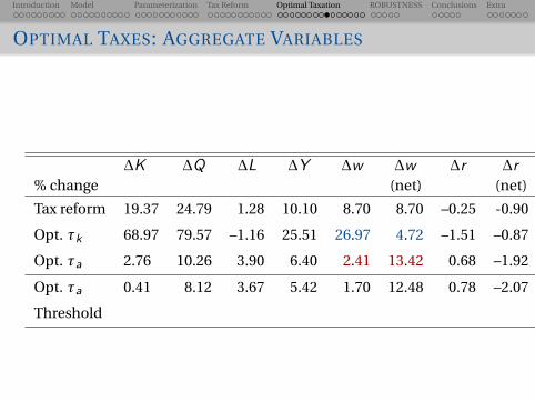
OPTIMAL TAXES: AGGREGATE VARIABLES
¢K ¢Q ¢L ¢Y ¢w ¢w ¢r ¢r% change (net) (net)
Tax reform 19.37 24.79 1.28 10.10 8.70 8.70 –0.25 -0.90
Opt. øk 68.97 79.57 –1.16 25.51 26.97 4.72 –1.51 –0.87
Opt. øa 2.76 10.26 3.90 6.40 2.41 13.42 0.68 –1.92
Opt. øa 0.41 8.12 3.67 5.42 1.70 12.48 0.78 –2.07
Threshold

Introduction Model Parameterization Tax Reform Optimal Taxation ROBUSTNESS Conclusions Extra
OPTIMAL TAXES: WELFARE
Baseline
øk ø` øa CE 2 Vote
(%) (%)
Benchmark 025% 22.4% – – –
Tax reform – 22.4% 1.13% 7.86
Opt. øk –34.4% 36.0% – 6.28
Opt. øa – 14.1% 3.06% 9.61
Opt. øa – 14.2% 3.30% 9.83
Threshold ThresholdE
= 25%
Introduction Model Parameterization Tax Reform Optimal Taxation ROBUSTNESS Conclusions Extra
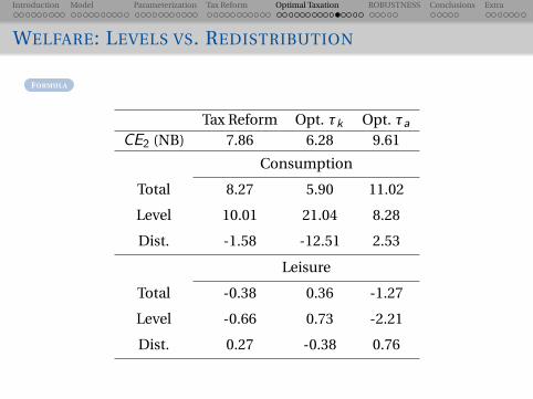
WELFARE: LEVELS VS. REDISTRIBUTION
FORMULA
Tax Reform Opt. øk Opt. øaCE2 (NB) 7.86 6.28 9.61
Consumption
Total 8.27 5.90 11.02
Level 10.01 21.04 8.28
Dist. -1.58 -12.51 2.53
Leisure
Total -0.38 0.36 -1.27
Level -0.66 0.73 -2.21
Dist. 0.27 -0.38 0.76
Introduction Model Parameterization Tax Reform Optimal Taxation ROBUSTNESS Conclusions Extra
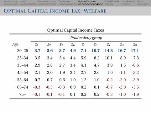
OPTIMAL CAPITAL INCOME TAX: WELFARE
Optimal Capital Income Taxes
Productivity group
Age z1 z2 z3 z4 z5 z6 z7 z8 z9
20–25 3.7 3.6 3.7 4.9 7.1 10.7 14.8 16.7 17.1
25–34 3.5 3.4 3.4 4.4 5.9 8.2 10.1 8.9 7.3
35–44 2.9 2.8 2.7 3.4 4.1 4.7 3.8 1.5 -0.6
45–54 2.1 2.0 1.9 2.4 2.7 2.6 1.0 -1.1 -3.2
55–64 0.7 0.7 0.6 1.0 1.2 1.0 -0.2 -2.0 -3.9
65–74 -0.3 -0.3 -0.3 0.0 0.2 0.1 -0.7 -2.0 -3.5
75+ -0.1 -0.1 -0.1 0.1 0.2 0.2 -0.3 -1.0 -1.9
Introduction Model Parameterization Tax Reform Optimal Taxation ROBUSTNESS Conclusions Extra
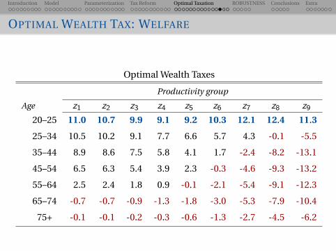
OPTIMAL WEALTH TAX: WELFARE
Optimal Wealth Taxes
Productivity group
Age z1 z2 z3 z4 z5 z6 z7 z8 z9
20–25 11.0 10.7 9.9 9.1 9.2 10.3 12.1 12.4 11.3
25–34 10.5 10.2 9.1 7.7 6.6 5.7 4.3 -0.1 -5.5
35–44 8.9 8.6 7.5 5.8 4.1 1.7 -2.4 -8.2 -13.1
45–54 6.5 6.3 5.4 3.9 2.3 -0.3 -4.6 -9.3 -13.2
55–64 2.5 2.4 1.8 0.9 -0.1 -2.1 -5.4 -9.1 -12.3
65–74 -0.7 -0.7 -0.9 -1.3 -1.8 -3.0 -5.3 -7.9 -10.4
75+ -0.1 -0.1 -0.2 -0.3 -0.6 -1.3 -2.7 -4.5 -6.2

Introduction Model Parameterization Tax Reform Optimal Taxation ROBUSTNESS Conclusions Extra
OPTIMAL WEALTH TAX WITH THRESHOLD: WELFARE
Optimal Wealth Taxes with Threshold
Productivity group
Age z1 z2 z3 z4 z5 z6 z7 z8 z9
20–25 10.5 10.3 9.8 9.3 9.5 10.6 12.4 12.6 11.4
25–34 10.1 9.9 9.0 7.8 6.7 5.7 4.2 -0.5 -6.3
35–44 8.6 8.4 7.4 5.8 4.1 1.5 -2.8 -9.0 -14.2
45–54 6.3 6.2 5.3 3.9 2.2 -0.5 -5.1 -10.0 -14.2
55–64 2.5 2.4 1.9 1.0 0.0 -2.1 -5.7 -9.6 -13.0
65–74 -0.5 -0.5 -0.6 -1.0 -1.5 -2.8 -5.3 -8.2 -10.9
75+ -0.1 -0.1 -0.1 -0.2 -0.4 -1.1 -2.7 -4.7 -6.5

Introduction Model Parameterization Tax Reform Optimal Taxation ROBUSTNESS Conclusions Extra
OPTIMAL TAXES: WELFARE
Baseline
øk ø` øa CE 2 Vote
(%) (%)
Benchmark 025% 22.4% – – –
Tax reform – 22.4% 1.13% 7.86 67.8
Opt. øk –34.4% 36.0% – 6.28 69.7
Opt. øa – 14.1% 3.06% 9.61 60.7
Opt. øa – 14.2% 3.30% 9.83 78.9
Threshold

Robustness

Introduction Model Parameterization Tax Reform Optimal Taxation ROBUSTNESS Conclusions Extra
TAX REFORM: AGGREGATES
% Change Baseline No Shock No Const. Prog. Labour Tax
k 19.37 9.56 6.28 21.27
Q 24.79 22.37 6.28 25.61
w 8.70 7.66 2.10 9.25
Y 10.10 9.54 3.02 10.01
L 1.28 1.75 0.91 0.69
C 10.01 11.25 2.93 10.01

Introduction Model Parameterization Tax Reform Optimal Taxation ROBUSTNESS Conclusions Extra
TAX REFORM: WELFARE
Baseline No Shock No Const. Prog. Labour Tax
Wealth Tax Rate 1.13% 1.23% 1.65% 0.90%
CE1 (All) 3.14 2.29 0.44 2.79
CE1 (NB) 7.40 5.46 1.86 6.48
CE2 (All) 5.14 2.92 0.36 4.68
CE2 (NB) 7.86 5.36 1.43 7.06

Introduction Model Parameterization Tax Reform Optimal Taxation ROBUSTNESS Conclusions Extra
OPTIMAL TAXES
øk ø` øa Top 1% CE 2 (%)
Baseline 25% 22.4% – 0.36
Opt. øk –34.4% 36.0% – 0.56 6.28
Opt. øa – 14.1% 3.06% 0.47 9.61
No Shock
Opt. øk -2.33% 29.0% – 0.47 3.27
Opt. øa – 18.5% 2.21% 0.46 5.80
No Constraint
Opt. øk 13.6% 26.0% – 0.39 0.41
Opt. øa – 22.7% 1.57% 0.42 1.43
Introduction Model Parameterization Tax Reform Optimal Taxation ROBUSTNESS Conclusions Extra
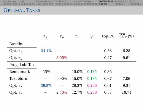
OPTIMAL TAXES
øk øa ø` √ Top 1% CE 2 (%)
Baseline
Opt. øk –34.4% – 0.56 6.28
Opt. øa – 3.06% 0.47 9.61
Prog. Lab. Tax
Benchmark 025% – 15.0% 0.185 0.36 –
Tax reform – 0.90% 15.0% 0.185 0.67 7.06
Opt. øk -38.8% – 29.3% 0.280 0.61 9.31
Opt. øa – 2.40% 12.7% 0.280 0.53 10.71

Introduction Model Parameterization Tax Reform Optimal Taxation ROBUSTNESS Conclusions Extra
COMPARISON TO EARLIER WORK
œ Conesa et al (AER, 2009) study optimal capital income taxes inincomplete markets OLG model
with idiosyncratic labor riskwithout return heterogeneityand find optimal øk = 36%increase in welfare of CE = 1.33%.
œ Why do we find optimal smaller øk or negative (but a large øw )?
In both Conesa et al and in our model, higher øk reduces capitalaccumulation and leads to lower output.However, in our model, higher øk hurts productive agentsdisproportionately, leading to more misallocation, and furtherreductions in output.With wealth tax, the tax burden is shared between productive andunproductive agents, leading to smaller misallocation and lowerdeclines in output with øa.

Introduction Model Parameterization Tax Reform Optimal Taxation ROBUSTNESS Conclusions Extra
CONCLUSIONS AND CURRENT WORK
œ Many countries currently have or have had wealth taxes:
France, Spain, Norway, Switzerland, Italy, Denmark, Germany,Finland, Sweden, among others.
œ However, the rationale for such taxes are often vague:
fairness, reducing inequality, etc...
and not studied formally
œ Here, we are proposing a case for wealth taxes entirely based onefficiency benefits and quantitatively evaluating its impact.

Introduction Model Parameterization Tax Reform Optimal Taxation ROBUSTNESS Conclusions Extra
CONCLUSIONS AND CURRENT WORK
œ Wealth tax has opposite implications of capital income tax.
œ Revenue neutral tax reform from øk to øa:
reallocates capital from less productive wealthy to the moreproductive wealthy.
gives the right incentives to the right people to save.
increases output, consumption, wages, and welfare.
Welfare gains are substantial.
œ Optimal wealth taxes are positive and large. Optimal capital taxesare negative or small.
Welfare gain is substantially larger under wealth taxes.

Introduction Model Parameterization Tax Reform Optimal Taxation ROBUSTNESS Conclusions Extra
CONCLUSIONS AND CURRENT WORK
œ Current work and extensions:
Complete the calibration of the stochastic component ofentrepreneurial productivity.
Optimize over consumption taxes.
Introduce estate taxes and study optimality vs. wealth taxes.
Are global wealth taxes necessary?

Introduction Model Parameterization Tax Reform Optimal Taxation ROBUSTNESS Conclusions Extra
Thanks!

Introduction Model Parameterization Tax Reform Optimal Taxation ROBUSTNESS Conclusions Extra
TABLE: Wealth Concentration by Asset Type
Stocks All stocks Non-equity Housing Net Worth
w/o pensions financial equity
Top 0.5% 41.4 37.0 24.2 10.2 25.6Top 1% 53.2 47.7 32.0 14.8 34.0Top 10% 91.1 86.1 72.1 51.7 68.7Bottom 90% 8.9 13.9 27.9 49.3 31.3
Gini Coefficients
Financial Wealth Net Worth
0.91 0.82
Source: Poterba (2000) and Wolff (2000)
BACK

Introduction Model Parameterization Tax Reform Optimal Taxation ROBUSTNESS Conclusions Extra
25 35 45 55 65 75 85
Year
9
9.5
10
10.5
11
Log10 (Real Net Worth) in $2015
Adelson
Bloomberg
Buffett
Cuban
Dell
Ellison
Gates
Charles Koch
Musk
Page
Paulson
Tepper
Jim Walton
Oprah
Zuckerberg
BACK

Introduction Model Parameterization Tax Reform Optimal Taxation ROBUSTNESS Conclusions Extra
Calendar Year
Name 80s 90s 00s 10s
Warren Buffett 44.37 18.57 0.02 5.81
Michael Dell 87.94 -5.58 2.97
Larry Ellison 54.09 31.31 4.90 8.06
Bill Gates 51.94 48.06 -7.54 5.46
Elon Musk 107.57
Larry Page 69.67 11.96
Mark Zuckerberg 33.81 62.24
BACK

Introduction Model Parameterization Tax Reform Optimal Taxation ROBUSTNESS Conclusions Extra
œ 1+CE = (1+CEC )(1+CEL)
œ CEC is given by
V0((1+CEC (s))c§US(s),`§US(s))= eV0(c(s),`§US(s))
CEC can be decomposed into level CEC and distrubutioncomponent CEæC as
V0((1+CEC (s))c§US(s),`§US(s))= bV0(bc(s),`§US(s))
where bc(s)= c(s) C
C§US
and
bV0 ((1+CEæC) bc(s),`§US(s))= eV0(c(s),`§US(s))
œ CEL is given by
V0((1+CEL(s))c§US(s),`§US(s))= eV0(c§US(s),`(s))
œ Similar decomposition applies to leisure.
BACK

Introduction Model Parameterization Tax Reform Optimal Taxation ROBUSTNESS Conclusions Extra
POLITICAL SUPPORT FOR WEALTH TAXES
Fraction with Positive Welfare Gain-Optimal Capital Inc. Tax
Productivity group
Age z1 z2 z3 z4 z5 z6 z7 z8 z9
20–25 0.96 0.95 0.95 0.98 0.99 0.99 0.99 0.99 0.99
25–34 0.97 0.97 0.96 0.98 0.97 0.96 0.94 0.90 0.85
35–44 0.95 0.94 0.92 0.95 0.93 0.88 0.80 0.68 0.58
45–54 0.88 0.88 0.86 0.89 0.85 0.78 0.66 0.53 0.43
55–64 0.68 0.67 0.68 0.72 0.69 0.62 0.52 0.41 0.31
65–74 0.09 0.05 0.14 0.22 0.22 0.21 0.18 0.15 0.11
75+ 0.12 0.12 0.13 0.15 0.15 0.15 0.13 0.11 0.09

Introduction Model Parameterization Tax Reform Optimal Taxation ROBUSTNESS Conclusions Extra
POLITICAL SUPPORT FOR WEALTH TAXES
Fraction with Positive Welfare Gain-Optimal Wealth Tax
Productivity group
Age z1 z2 z3 z4 z5 z6 z7 z8 z9
20–25 0.97 0.97 0.95 0.93 0.93 0.94 0.93 0.90 0.87
25–34 0.98 0.98 0.96 0.93 0.90 0.86 0.77 0.59 0.43
35–44 0.97 0.97 0.94 0.87 0.80 0.66 0.48 0.35 0.27
45–54 0.93 0.93 0.88 0.79 0.68 0.55 0.42 0.32 0.25
55–64 0.73 0.72 0.67 0.59 0.51 0.41 0.33 0.25 0.19
65–74 0.00 0.02 0.01 0.02 0.01 0.01 0.01 0.00 0.00
75+ 0.00 0.00 0.04 0.03 0.02 0.02 0.01 0.01 0.00
Introduction Model Parameterization Tax Reform Optimal Taxation ROBUSTNESS Conclusions Extra
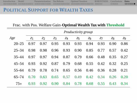
POLITICAL SUPPORT FOR WEALTH TAXES
Frac. with Pos. Welfare Gain-Optimal Wealth Tax with Threshold
Productivity group
Age z1 z2 z3 z4 z5 z6 z7 z8 z9
20–25 0.97 0.97 0.95 0.93 0.93 0.94 0.93 0.90 0.86
25–34 0.98 0.98 0.96 0.93 0.90 0.85 0.77 0.57 0.42
35–44 0.97 0.97 0.94 0.87 0.79 0.66 0.48 0.35 0.27
45–54 0.93 0.92 0.87 0.79 0.68 0.55 0.42 0.32 0.25
55–64 0.79 0.78 0.74 0.65 0.56 0.46 0.36 0.28 0.21
65–74 0.70 0.63 0.65 0.57 0.49 0.42 0.34 0.26 0.20
75+ 0.93 0.92 0.90 0.84 0.78 0.68 0.55 0.43 0.34