Embed Size (px)
Citation preview

Development of Integrated Urban System Models: Population
Life-transitions, Household location, and Vehicle Transaction
Decisions
by
Mahmudur Rahman Fatmi
Submitted in partial fulfillment of the requirements
for the degree of Doctor of Philosophy
at
Dalhousie University
Halifax, Nova Scotia
November 2017
© Copyright by Mahmudur Rahman Fatmi, 2017
ii
DEDICATION
To My Father, Late Md. Wajiur Rahman
&
My Mother, Fatema Rahman
iii
Table of Contents
List of Tables ................................................................................................ viii
List of Figures .................................................................................................. x
Abstract .................................................................................................. xiv
List of Abbreviations Used ............................................................................. xv
Acknowledgements ........................................................................................ xvi
Chapter 1 Introduction ................................................................................. 1
1.1 Background and Motivation .......................................................... 1
1.2 Objectives ....................................................................................... 4
1.3 Significance .................................................................................... 4
1.4 Thesis Outline ................................................................................ 5
Chapter 2 Literature Review ........................................................................ 7
2.1 Introduction ................................................................................... 7
2.2 Typology of Integrated Urban Models .......................................... 8
2.2.1 Economic Activity-based Models ..................................................... 9
2.2.2 Market Principle Models ............................................................... 10
2.2.3 Quasi Market-based Models .......................................................... 13
2.2.4 Hybrid Models of Heuristic, Utility, and Market
Principles ....................................................................................... 15
2.2.5 Emerging Complex System Models .............................................. 18
2.3 Modelling Location Choice, Mode Transition, and Vehicle
Transaction Decisions ................................................................. 21
2.3.1 Modelling Residential Location ..................................................... 21
2.3.2 Modelling Commute Mode Transitions......................................... 23
iv
2.3.3 Modelling Vehicle Transactions .................................................... 26
2.4 Issues in the Existing Integrated Urban Models ....................... 28
2.5 Research Questions and Concluding Remarks .......................... 31
Chapter 3 Conceptual Framework and Data ............................................. 33
3.1 Theoretical Context ..................................................................... 33
3.2 Modelling Framework of the Proposed Integrated Urban
Model ........................................................................................... 35
3.2.1 Baseline Synthesis ......................................................................... 37
3.2.2 Population Life-stage Transition .................................................. 37
3.2.3 Residential Location Transition .................................................... 37
3.2.4 Vehicle Ownership Transition ...................................................... 38
3.2.5 Activity-based Travel ..................................................................... 39
3.2.6 Population and Urban Form Representation ............................... 39
3.3 Data Sources and Description ..................................................... 40
3.3.1 Retrospective Survey Data ............................................................ 40
3.3.2 Secondary Data Sources ................................................................ 43
3.4 Derived Independent Variables .................................................. 46
3.4.1 Life-cycle Events ............................................................................ 46
3.4.2 Accessibility Measures .................................................................. 47
3.4.3 Land Use and Neighbourhood Characteristics ............................ 47
3.4.4 Socio-demographic and Dwelling Characteristics ........................ 48
3.5 Conclusions .................................................................................. 48
Chapter 4 Modelling Residential Location Processes ................................. 50
4.1 Introduction ................................................................................. 50
4.2 Residential Mobility .................................................................... 53
v
4.2.1 Methodology ................................................................................... 53
4.2.2 Discussion of Model Results .......................................................... 57
4.3 Residential Location Choice ........................................................ 61
4.3.1 Methodology ................................................................................... 62
4.3.2 Goodness-of-fit Measures .............................................................. 75
4.3.3 Discussion of Model Results .......................................................... 79
4.4 Modelling Mode Transitions ....................................................... 85
4.4.1 Modelling Methods ........................................................................ 85
4.4.2 Model Results ................................................................................. 89
4.5 Conclusions and Summary of Contributions ............................ 103
Chapter 5 Modelling Vehicle Transactions .............................................. 109
5.1 Introduction ............................................................................... 109
5.2 Modelling Methods .................................................................... 110
5.3 Model Results ............................................................................ 112
5.3.1 Results of the Segment Allocation Model ................................... 116
5.3.2 Discussion of the Latent Segmentation-based Logit
(LSL) Model Results .................................................................... 117
5.4 Conclusions and Summary of Contributions ............................ 123
Chapter 6 Baseline Synthesis and Microsimulation of Life-stage
Transitions .............................................................................. 126
6.1 Introduction ............................................................................... 126
6.2 Implementation of the iTLE Proto-type Model ........................ 127
6.3 Population Synthesis ................................................................. 128
6.3.1 Synthesis Process......................................................................... 128
6.3.2 Synthesis Results ......................................................................... 130

vi
6.4 Vehicle Ownership Level Synthesis .......................................... 134
6.4.1 Model Estimation ......................................................................... 134
6.4.2 Vehicle Ownership Level Synthesis Results .............................. 136
6.5 Population Life-stage Transition Module ................................. 137
6.5.1 Microsimulation Process ............................................................. 137
6.5.2 Validation Results ....................................................................... 139
6.5.3 Microsimulation Results .............................................................. 144
6.6 Conclusions and Summary of Contributions ............................ 145
Chapter 7 Microsimulation of Residential Location Processes ................. 148
7.1 Introduction ............................................................................... 148
7.2 Microsimulation Processes ........................................................ 149
7.2.1 Residential Mobility .................................................................... 149
7.2.2 Residential Location Choice ........................................................ 150
7.3 Validation Results ..................................................................... 151
7.4 Predicted Evolution of the Halifax Population Behaviour ...... 152
7.4.1 Predicted Evolution of Duration of Stay ..................................... 152
7.4.2 Predicted Evolution of the Spatial Distribution of the
Halifax Population ....................................................................... 157
7.4.3 Predicted Demographic Composition of the High
Density Neighbourhoods in Halifax ............................................ 159
7.5 Conclusions and Summary of Contributions ............................ 166
Chapter 8 Microsimulation of Vehicle Transactions ................................ 169
8.1 Introduction ............................................................................... 169
8.2 Microsimulation Processes ........................................................ 170
8.2.1 Vehicle Ownership State ............................................................. 170
vii
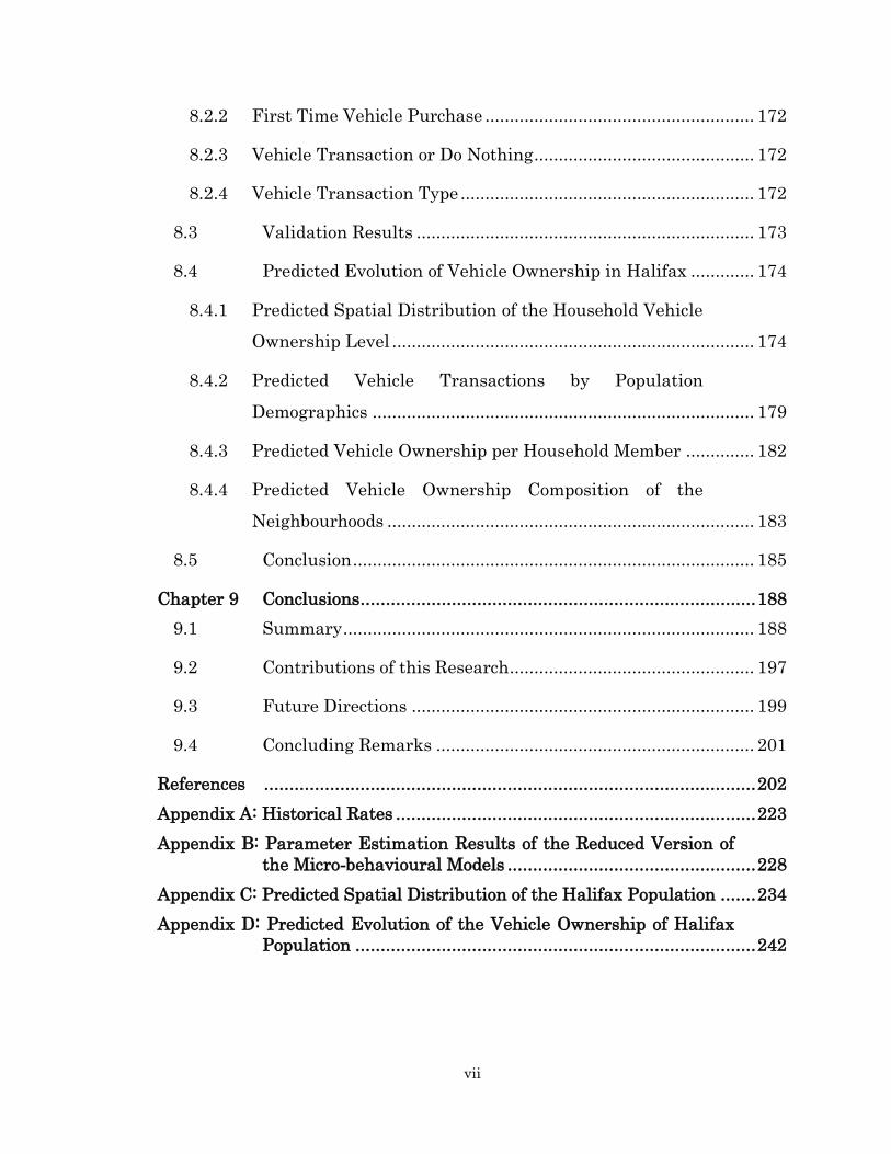
8.2.2 First Time Vehicle Purchase ....................................................... 172
8.2.3 Vehicle Transaction or Do Nothing ............................................. 172
8.2.4 Vehicle Transaction Type ............................................................ 172
8.3 Validation Results ..................................................................... 173
8.4 Predicted Evolution of Vehicle Ownership in Halifax ............. 174
8.4.1 Predicted Spatial Distribution of the Household Vehicle
Ownership Level .......................................................................... 174
8.4.2 Predicted Vehicle Transactions by Population
Demographics .............................................................................. 179
8.4.3 Predicted Vehicle Ownership per Household Member .............. 182
8.4.4 Predicted Vehicle Ownership Composition of the
Neighbourhoods ........................................................................... 183
8.5 Conclusion .................................................................................. 185
Chapter 9 Conclusions .............................................................................. 188
9.1 Summary .................................................................................... 188
9.2 Contributions of this Research .................................................. 197
9.3 Future Directions ...................................................................... 199
9.4 Concluding Remarks ................................................................. 201
References ................................................................................................. 202
Appendix A: Historical Rates ....................................................................... 223
Appendix B: Parameter Estimation Results of the Reduced Version of
the Micro-behavioural Models ................................................. 228
Appendix C: Predicted Spatial Distribution of the Halifax Population ....... 234
Appendix D: Predicted Evolution of the Vehicle Ownership of Halifax
Population ............................................................................... 242
viii
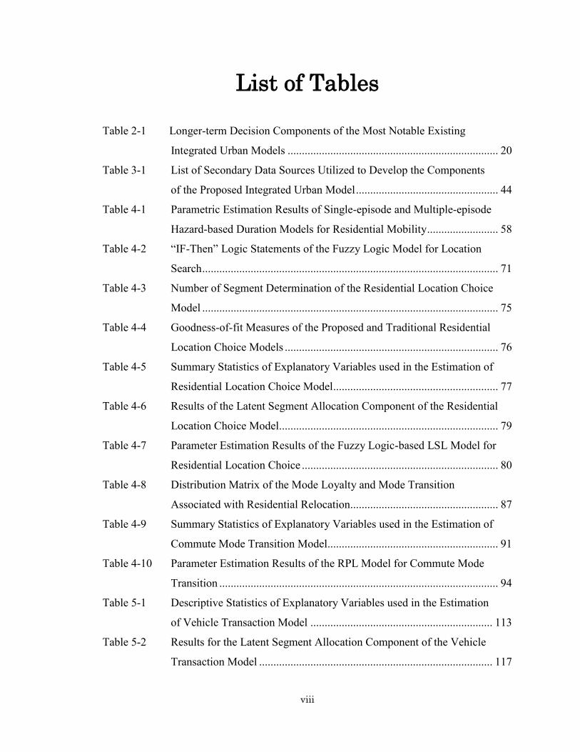
List of Tables
Table 2-1 Longer-term Decision Components of the Most Notable Existing
Integrated Urban Models .......................................................................... 20
Table 3-1 List of Secondary Data Sources Utilized to Develop the Components
of the Proposed Integrated Urban Model .................................................. 44
Table 4-1 Parametric Estimation Results of Single-episode and Multiple-episode
Hazard-based Duration Models for Residential Mobility ......................... 58
Table 4-2 “IF-Then” Logic Statements of the Fuzzy Logic Model for Location
Search ........................................................................................................ 71
Table 4-3 Number of Segment Determination of the Residential Location Choice
Model ........................................................................................................ 75
Table 4-4 Goodness-of-fit Measures of the Proposed and Traditional Residential
Location Choice Models ........................................................................... 76
Table 4-5 Summary Statistics of Explanatory Variables used in the Estimation of
Residential Location Choice Model.......................................................... 77
Table 4-6 Results of the Latent Segment Allocation Component of the Residential
Location Choice Model ............................................................................. 79
Table 4-7 Parameter Estimation Results of the Fuzzy Logic-based LSL Model for
Residential Location Choice ..................................................................... 80
Table 4-8 Distribution Matrix of the Mode Loyalty and Mode Transition
Associated with Residential Relocation.................................................... 87
Table 4-9 Summary Statistics of Explanatory Variables used in the Estimation of
Commute Mode Transition Model............................................................ 91
Table 4-10 Parameter Estimation Results of the RPL Model for Commute Mode
Transition .................................................................................................. 94
Table 5-1 Descriptive Statistics of Explanatory Variables used in the Estimation
of Vehicle Transaction Model ................................................................ 113
Table 5-2 Results for the Latent Segment Allocation Component of the Vehicle
Transaction Model .................................................................................. 117
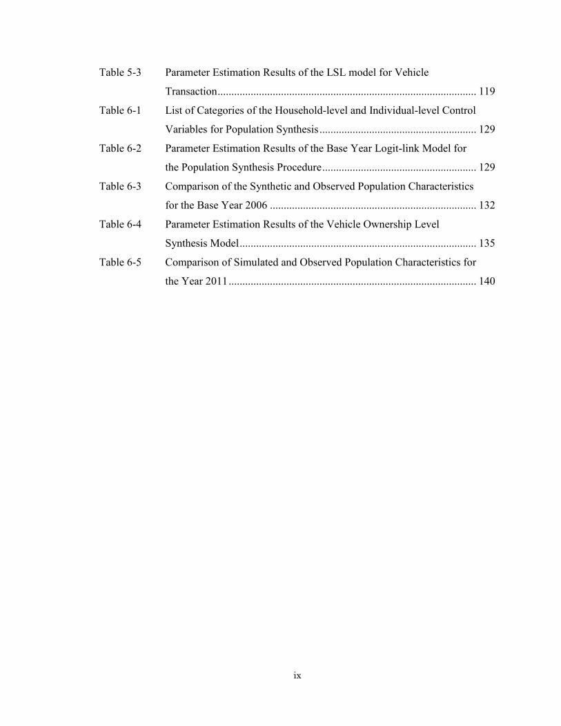
ix
Table 5-3 Parameter Estimation Results of the LSL model for Vehicle
Transaction .............................................................................................. 119
Table 6-1 List of Categories of the Household-level and Individual-level Control
Variables for Population Synthesis ......................................................... 129
Table 6-2 Parameter Estimation Results of the Base Year Logit-link Model for
the Population Synthesis Procedure ........................................................ 129
Table 6-3 Comparison of the Synthetic and Observed Population Characteristics
for the Base Year 2006 ........................................................................... 132
Table 6-4 Parameter Estimation Results of the Vehicle Ownership Level
Synthesis Model ...................................................................................... 135
Table 6-5 Comparison of Simulated and Observed Population Characteristics for
the Year 2011 .......................................................................................... 140
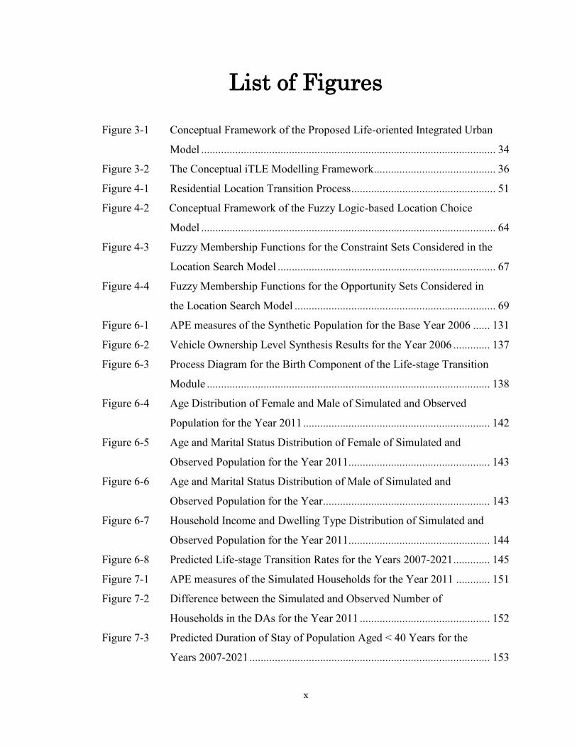
x
List of Figures
Figure 3-1 Conceptual Framework of the Proposed Life-oriented Integrated Urban
Model ........................................................................................................ 34
Figure 3-2 The Conceptual iTLE Modelling Framework........................................... 36
Figure 4-1 Residential Location Transition Process ................................................... 51
Figure 4-2 Conceptual Framework of the Fuzzy Logic-based Location Choice
Model ........................................................................................................ 64
Figure 4-3 Fuzzy Membership Functions for the Constraint Sets Considered in the
Location Search Model ............................................................................. 67
Figure 4-4 Fuzzy Membership Functions for the Opportunity Sets Considered in
the Location Search Model ....................................................................... 69
Figure 6-1 APE measures of the Synthetic Population for the Base Year 2006 ...... 131
Figure 6-2 Vehicle Ownership Level Synthesis Results for the Year 2006 ............. 137
Figure 6-3 Process Diagram for the Birth Component of the Life-stage Transition
Module .................................................................................................... 138
Figure 6-4 Age Distribution of Female and Male of Simulated and Observed
Population for the Year 2011 .................................................................. 142
Figure 6-5 Age and Marital Status Distribution of Female of Simulated and
Observed Population for the Year 2011 .................................................. 143
Figure 6-6 Age and Marital Status Distribution of Male of Simulated and
Observed Population for the Year ........................................................... 143
Figure 6-7 Household Income and Dwelling Type Distribution of Simulated and
Observed Population for the Year 2011 .................................................. 144
Figure 6-8 Predicted Life-stage Transition Rates for the Years 2007-2021 ............. 145
Figure 7-1 APE measures of the Simulated Households for the Year 2011 ............ 151
Figure 7-2 Difference between the Simulated and Observed Number of
Households in the DAs for the Year 2011 .............................................. 152
Figure 7-3 Predicted Duration of Stay of Population Aged < 40 Years for the
Years 2007-2021 ..................................................................................... 153
xi
Figure 7-4 Predicted Duration of Stay of Population Aged 40-54 Years for the
Years 2007-2021 ..................................................................................... 154
Figure 7-5 Predicted Duration of Stay of Population Aged 55-64 Years for the
Years 2007-2021 ..................................................................................... 154
Figure 7-6 Predicted Duration of Stay of Population Aged > 64 Years for the
Years 2007-2021 ..................................................................................... 155
Figure 7-7 Predicted Duration of Stay of Population by Age and Location of the
Residence for the Years 2007-2021 ........................................................ 156
Figure 7-8 Predicted Duration of Stay of Population by Household Income and
Location of Residence for the Years 2007-2021 .................................... 156
Figure 7-9 Predicted Household Density Change from 2006 to 2021...................... 157
Figure 7-10 Predicted Spatial Distribution of the Halifax Population for the Year
2021......................................................................................................... 158
Figure 7-11 Predicted Yearly Avg. Household Density of the High Density DAs in
Halifax for the Years 2007-2021 ............................................................ 159
Figure 7-12 Predicted Yearly Avg. HH Income in Low Income High Density DAs
in Halifax for the Years 2007-2021 ........................................................ 160
Figure 7-13 Predicted Yearly Avg. HH Income in High Income High Density DAs
in Halifax for the Years 2007-2021 ........................................................ 161
Figure 7-14 Predicted Yearly Avg. Age of HH Head in Low Income High Density
DAs in Halifax for the Years 2007-2021 ................................................ 162
Figure 7-15 Predicted Yearly Avg. Age of HH Head in High Income High Density
DAs in Halifax for the Years 2007-2021 ................................................ 162
Figure 7-16 Predicted Distribution of Single Person HH in the High Density
Neighbourhoods of Halifax for the Year 2021 ....................................... 164
Figure 7-17 Predicted Distribution of Couple without Child HH in the High
Density Neighbourhoods of Halifax for the Year 2021 .......................... 164
Figure 7-18 Predicted Distribution of Couple with One Child HH in the High
Density Neighbourhoods of Halifax for the Year 2021 .......................... 165
Figure 7-19 Predicted Distribution of Couple with Two Child HH in the High
Density Neighbourhoods of Halifax for the Year 2021 .......................... 165
xii
Figure 7-20 Predicted Distribution of Couple with more than Two Child HH in the
High Density Neighbourhoods of Halifax for the Year 2021 ................. 166
Figure 8-1 Operational Framework of the Vehicle Transaction Component of
iTLE ........................................................................................................ 171
Figure 8-2 Vehicle Ownership Level Comparison of the Predicted and Observed
Halifax Population for the Year 2016 ..................................................... 174
Figure 8-3 Predicted Distribution of Vehicle Ownership Level by Home Location
for the Year 2007 .................................................................................... 175
Figure 8-4 Predicted Spatial Distribution of Zero Vehicle Ownership Households
in the DA for the Year 2021 ................................................................... 177
Figure 8-5 Predicted Spatial Distribution of One Vehicle Ownership Households
in the DA for the Year 2021 ................................................................... 177
Figure 8-6 Predicted Spatial Distribution of Two Vehicle Ownership Households
in the DA for the Year 2021 ................................................................... 178
Figure 8-7 Predicted Spatial Distribution of Three or More Vehicle Ownership
Households in the DA for the Year 2021 ................................................ 178
Figure 8-8 Predicted Distribution of Age and Income of Households Purchasing
First Vehicle for the Year 2021 .............................................................. 180
Figure 8-9 Predicted Distribution of Age and Income of Households Acquiring
Vehicles for the Year 2021 ..................................................................... 180
Figure 8-10 Predicted Distribution of Age and Income of Households Disposing
Vehicles for the Year 2021 ..................................................................... 181
Figure 8-11 Predicted Distribution of Age and Income of Households Trading
Vehicles for the Year 2021 ..................................................................... 181
Figure 8-12 Predicted Spatial Distribution of Vehicle Ownership per Household
Member by Income for the Year 2021 .................................................... 182
Figure 8-13 Predicted Spatial Distribution of Vehicle Ownership per Household
Member by Age for the Year 2021 ......................................................... 183
Figure 8-14 Predicted 15 Year Evolution of Average Vehicle Ownership per
Household in the DA for the Years 2007-2021 ...................................... 184
xiii
Figure 8-15 Predicted Spatial Distribution of the Avg. Vehicle Ownership per
Household in the DA by Avg. Household Income in the DA for the
Year 2021 ................................................................................................ 185

xiv
Abstract
This research presents the development of a life-oriented, agent-based
integrated transport land use and energy (iTLE) model. A life-oriented theory
and perspective is adopted to accommodate life-trajectory dynamics of key
longer-term household-level decisions within the integrated urban modelling
system. This study develops the following components of the proposed
integrated urban model: population synthesis, vehicle ownership level
synthesis, life-stage transition, residential location, vehicle transaction, and
mode transition. The modelling and computation procedure of the integrated
model addresses evolution of location choice and vehicle transaction over the
life-course of the households in response or anticipation to decisions and
changes at different life-domains. One of the mechanisms adopted to
accommodate the temporal dimension of such multi-way decision interactions
is through introducing lead and lag events. Advanced econometric models are
developed to accommodate the effects of repeated choices during the life-course
of the households, as well as capture unobserved heterogeneity. For example,
a dynamic vehicle transaction model is developed utilizing a latent
segmentation-based logit (LSL) modelling technique. Moreover, residential
location and vehicle transaction are assumed to have an underlying process
orientation. For instance, residential location is conceptualized as a two-stage
process of: 1) mobility, and 2) location choice. Methodologically, the second
stage of location choice is modelled as a two-tier process of location search and
choice, by utilizing a fuzzy logic-based modelling method and LSL modelling
technique. Vehicle transaction is modelled as a process of first time purchase,
acquisition, disposal, and trade. Finally, this research implements a proto-type
version of the iTLE model for Halifax, Canada. The proto-type generates a
synthesis-based population and vehicle ownership level information for the
base year 2006. The model microsimulates life-stage transition, residential
location, and vehicle transaction for a 15-year period of 2007-2021. This
research also presents validation of the iTLE proto-type model results, and
predicts the evolution of life-stage, mobility, location, and vehicle transaction
for the Halifax population. This simulation modelling system would be useful
for analyzing complex, integrated land use and transport policy scenarios.
xv
List of Abbreviations Used
APE Absolute Percent Error
BIC Bayesian Information Criteria
CBD Central Business District
DA Dissemination Area
DMTI Desktop Mapping Technologies Inc.
HMTS Household Mobility and Travel Survey
HRM Halifax Regional Municipality
IPU Iterative Proportional Updating
iTLE integrated Transport Land Use and Energy Model
IUM Integrated Urban Model
LSL Latent Segmentation-based Logit
NovaTRAC Nova Scotia Travel Activity Survey
PUMF Public Use Microdata File
RPL Random-parameters Logit
SRMSE Standard Root Mean Square Error
xvi
Acknowledgements
I am grateful to a number of people for their generous support, advise,
friendship, and encouragement during my tenure as a PhD student. First, I
would like to thank my supervisor, Prof. Dr. Ahsan Habib for giving me the
opportunity to sail for this tremendous journey with him, which has been a
great honour for me. Starting from my masters in 2012, past five years work
experience with Prof. Habib has matured me as a researcher, more
importantly, as a human being. I don’t know whether I would ever be able to
thank you enough for supporting me, for sharing your knowledge, for providing
me a wide array of research opportunities and attend conferences, for endlessly
encouraging me to publish, for offering me teaching opportunity, for being
easily accessible, for your valuable suggestions, for being enthusiastic to my
every crazy research ideas, and for planting in me the confidence that yes I
can. To me, you have been a supervisor, a teacher, a friend, and a guide, who
encourages me to thrive in life. Thanks for believing in me more than I believed
myself.
I would like to thank my doctoral supervisory committee members: Prof.
Nouman Ali, and Prof. William Phillips for your insightful comments and
valuable suggestions at different stages of my research. Your critical reviews
have helped me greatly to improve the thesis. Thanks to Prof. Ali for giving me
the opportunity to instruct a Civil Engineering course, which has been a
fantastic experience in many ways. Thanks to Prof. Phillips for providing me
the opportunity to help you in teaching Engineering Mathematics courses.
Special thanks to my external examiner Prof. Mathew Roorda for offering your
valuable time. Your thoughtful reviews have helped me to improve this
dissertation.

xvii
I would like to thank my colleagues at DalTRAC, including Robin, Jahed, Sara,
Pauline, Claire, Cara, Siobhan, Leen, Stephen, Nikki, Chris, Mateja, Nick,
Stephanie, and Sourov. A big shout-out to Robin and Jahed for being my
younger brothers. I would like to thank DalTRAC programmer Sourov for your
efforts in coding different components of the iTLE model. Thanks to Sara for
always managing time to proofread my papers. A big thanks to my friends in
Halifax, with whom I have shared numerous stimulating conversations at the
Tim Horton’s.
I would like to thank my parents, my siblings (Julie, Rimi, and Akib), niece
(Sinin, Tultul, and Rimjhim), and nephew (Siam) for their love and support.
Last but not the least, I would like to thank my wife, Shamsad Irin, who finally
figured out that I am actually a nerd trying to be flamboyant. Thanks for your
endless support, encouragement, love, and patience. I found you steadfast in
all the ups and downs in our life. Without you, this work would not have been
possible for me to complete.
1
Chapter 1
1 Introduction
1.1 Background and Motivation
The increasing urban sprawl and dependence on private vehicles posit
challenges for planning healthy communities, and promote equitable and
sustainable travel opportunities for people. Since location and travel choices
are inter-dependent decisions, effective integrated transport and land use
policies are required to trigger a shift towards balanced urban growth and
sustainable travel choices for the current population and generations to come.
Integrated urban models facilitate a modelling platform to effectively evaluate
complex land use and transport policies, since large-scale urban models
simulate the essential decision processes of the individuals/households to
represent the evolution of urban form and transport. Therefore, the
development of integrated urban models have emerged from the need to mimic
such two-way interactions between land use and transport.
In addition to the two-way inter-dependency, there exists a multi-way decision
interactions as travel behaviour and location choice evolve in response or
anticipation to decisions and changes at different life-domains. For example,
the decisions of where to live, where to work, how many vehicles to own, and
what mode to choose, interacts with each other. Although the interaction
between land use and transport is well recognized within the existing models,
such as UrbanSim, ILUTE, and PUMA (Waddell 2002, Salvini and Miller 2005,
Ettema et al. 2007); the evolving life-oriented interactions among the multi-
domain decisions have not been well addressed within the integrated urban
modelling literature. Life-history, its evolution, and influence on different
2
essential decision processes need to be addressed within the integrated urban
models as these models simulate individuals’ decisions over a long multi-year
time frame. During this period, individuals’ demographic career evolves, such
as a single person become married, have children, get divorced, and finally
decease. A change in the demographic status influences individuals’ decisions
at different life-domains. For example, birth of a child influences residential
location choices (Strom 2010), as well as vehicle transactions (Oakil et al.
2014). To adequately address the decision dynamics, population life-course and
associated changes are required to evolve within the simulation environment
of the integrated models. Hence, it is imperative for integrated models to
respond to the changes across the agents’ life-stages, starting with the long-
term and medium-term decisions, and life-stage transitions.
Among the several components of an integrated urban model, location choice,
vehicle ownership, and mode choice, are critical elements. Residential location
is a long-term decision (Habib 2009), which predicts the spatial distribution of
an urban region. Location choice decisions have an inherent process
orientation. For instance, residential location is a process of decision to move
(i.e. mobility) and location choice. Following the decision to move, households
chooses a location to move in, which itself can be characterized as a two-tier
process of home search and location choice. In this process, first households
undertake a search process to identify a pool of potential location alternatives
and finally choose a location from the pool. However, the process orientation of
the decisions are rarely accommodated within the operational integrated
urban models. In addition, an important dimension is to examine how a change
in the long-term state such as residential location influences travel activities
such as commute mode choice.
Another critical component of integrated models is medium-term decisions
such as vehicle ownership that directly influences short-term decisions of
travel activity. Vehicles are a major source of greenhouse gas (GHG) emission.
3
In Canada, a quarter of the total GHG emission is from the transportation
sector (Environment Canada 2014). The forecasting of vehicle ownership offers
the opportunity to test the impacts of strategies targeting the promotion of
sustainable travel choices, such as use of fuel efficient vehicles, and use of
alternative/clean fuel vehicles, among others. However, limited of the existing
urban models include vehicle ownership component. Furthermore, vehicle
ownership decisions have an underlying process orientation, since households
add, dispose, and trade vehicles. Hence, it is not only necessary to
microsimulate vehicle ownership within the integrated urban modelling
platform, but also required to address the process orientation of the
phenomenon.
The motivation of this research is to mimic the multi-domain interactions and
process orientation of the household-level decisions within an integrated urban
modelling system. This study presents the development of a proto-type, life-
oriented integrated Transport Land Use and Energy (iTLE) model. The iTLE
is an agent-based model that follows life-course perspectives and theories
(Chatterjee and Scheiner 2015). Life-course perspectives focus on how
transitions along the life-time and interactions among decisions taken at
different domains along the life-course influence individuals’ choices and
behaviour (Chatterjee and Scheiner 2015, Zhang 2017, Zhang 2015). The iTLE
simulates agents’ decisions longitudinally at each simulation time-step along
their life-course. The process orientation and multi-domain interaction among
the decisions are addressed within the micro-modelling structures and
computational procedures of the iTLE. This research addresses the
development of the following core components of iTLE: life-stage transition,
residential location, vehicle transaction, and mode transition. In addition, the
study generates baseline information including, population synthesis, and
vehicle ownership level synthesis. This research also offers predicted spatio-
temporal evolution of the urban population for the Halifax Regional

4
Municipality, in-terms of their demographic distribution, housing pattern,
neighbourhood composition, and vehicle ownership and transaction
configuration.
1.2 Objectives
The goal of this thesis is to develop a state-of-the-art agent-based integrated
urban model that addresses the process orientation and interactions among a
number of decisions along the life-course of the agents within the empirical
and microsimulation environment. To achieve this goal, the specific objectives
of this thesis evolves within the following four dimensions:
1. To develop micro-models of household location processes, including
residential mobility, location choice, and commute mode transition
associated with relocation.
2. To develop econometric models of vehicle transaction processes, such as
first time vehicle purchase, acquisition, disposal, and trade.
3. To generate baseline synthesis, life-stage transition, and proto-type
implementation of household decision processes within a life-oriented
urban systems model.
4. To predict micro-level spatio-temporal evolution of an urban region by
utilizing integrated urban systems model.
1.3 Significance
The contribution of this research encompasses the modelling and
microsimulation paradigms of the integrated urban modelling literature. It has
theoretical as well as applied implications. From a theoretical perspective, this
study adopts a life-oriented approach to investigate how decisions in different
life-domains such as location choice, vehicle ownership, and mode choice

5
interact along the life-course of the individuals/households. The investigation
provides important behavioural insights towards understanding of how
changes along the life-course shapes individuals/households behaviour. The
process orientation of the decisions are addressed within the modelling
framework through utilizing innovative modelling techniques. Developing
such advanced mathematical models that also warrants improved empirical
results significantly contributes to the literature of travel demand modelling
techniques.
In terms of the applied implications, this research is one of the first attempts
to translate the multi-directional interactions and process orientation of the
decisions from the micro-behavioural models to the computational procedure
of integrated urban models. Such multi-way feedback mechanisms within the
simulation environment of an urban model adds the capacity to test the
response of population at different life-stages under alternative land use and
transport policy scenarios. Particularly, this research microsimulates
individuals/households life-stages, residential location, and vehicle transaction
decisions within an agent-based integrated urban modelling system. The
microsimulation results offer insights towards the micro-level spatio-temporal
evolution of an urban region, including demographic distribution, housing
pattern, neighbourhood configuration, and vehicle ownership pattern. Such
information will be useful inputs for the development of a state-of-the-art
activity-based travel model. The findings have important implications towards
making effective integrated land use and transport policies.
1.4 Thesis Outline
This thesis is comprised of nine chapters. Chapter two reviews the relevant
literatures, including a typology of the integrated urban models, followed by
literature review on modelling residential location, mode transition, and
6
vehicle transaction decisions. This chapter concludes with a summary of the
literature review to identify research gaps, and then poses research questions
and concluding remarks.
Chapter three discusses the conceptual framework and data used to develop
an integrated urban model for Halifax. This chapter also provides details on
the independent variables considered during the model estimation processes
of different components of the urban model.
Chapter four describes the methods and results of modelling residential
location processes. Discussions on modelling residential mobility, location
search, location choice, and mode transition decisions are presented in this
chapter.
Chapter five provides the modelling methods and estimation results of the
vehicle transaction model.
Chapter six presents the development of a proto-type version of the iTLE model
for Halifax, Canada. This chapter focuses on the results of microsimulating
life-stages, and generating baseline synthesis information including
population and vehicle ownership level synthesis.
Chapter seven provides the details on microsimulating residential location
within the iTLE model. This chapter discusses the spatial and temporal
evolution of housing pattern and neighbourhood composition of Halifax.
Chapter eight presents the microsimulation results of the vehicle transaction
component of the iTLE model.
Finally, chapter nine summarizes the research findings and list of
contributions, and offers insights towards future research directions.
7
Chapter 2
2 Literature Review
2.1 Introduction
This research attempts to fill some gaps in the existing literature of modelling
and microsimulating residential location and vehicle transaction decisions
within an integrated urban modelling system. Integrated urban models
(alternatively termed as IUM in this study) are large-scale modelling systems
that simulate population’s decisions to predict the evolution of urban form and
transport. The potential of IUMs in enhancing the effective evaluation of
complex land use and transport policies have resulted in the development of
several large-scale models, such as ILUTE, UrbanSim, PUMA, SelfSim, and
SimMobility, among others. The components of IUMs can be categorized into
long-term decision models (e.g. location choice), medium-term decision models
(e.g. vehicle ownership), and short-term decision models (e.g. mode choice).
Long-term and medium-term decisions are critical components of an IUM
which have a dynamic nature, as these decisions interact with each other. For
example, the decision of where to live influences the decision of how many
vehicle to own, and vice-versa (Rashidi and Mohammadian 2011). These
crucial decisions evolve over the life-course as well as interact with life-stage
transitions; for instance, birth of a child influences residential location choices
(Strom 2010). Majority of the IUMs do not tackle such multi-domain
interactions among decisions taken at different life-stages of the population.
Although significant advances is made in developing the short-term models,
also known as the transport component of the IUMs; one of the criticisms of
most of the IUMs has been the lack of behavioural representation for the long-
term and medium-term models. To effectively evaluate land use and transport

8
policies, integrated urban models need to be responsive to the decision
dynamics across the agents’ decision making domains and life-stages. The
empirical settings as well as the computation procedure of the IUMs are
required to accommodate the multi-way feedback mechanism among the
decision processes.
This chapter reviews relevant literatures on integrated urban models and
modelling of essential decision processes to identify the scope for this research.
First, a typology of the existing integrated urban models with a brief
description is presented. Then, a review of modelling longer-term decision
processes including residential location choice followed by mode transition and
vehicle transaction are described. After that a discussion on the modelling
issues of the existing integrated urban models is presented. Finally, some
research questions are formulated, which pegs the scope for the contributions
of this research.
2.2 Typology of Integrated Urban Models
To-date, a number of integrated urban models are developed, starting from the
Lowry model (Lowry 1964) in early 1960s to the recent SelfSim (Zhuge et al.
2016) model. A number of review articles on integrated urban models already
exist (Huang et al. 2014, Iacono et al. 2008, Hunt et al. 2005, Miller 2009,
Wegener 2004, Timmermans 2003). This section reviews the recent
developments and updates on the most noteworthy models that are currently
available. Based on the operating principles, IUMs can be subdivided into the
following five categories: (1) Economic Activity-based Models, (2) Market
Principle Models, (3) Quasi Market-based Models, (4) Hybrid Models of
Heuristic, Utility, and Market Principles, and (5) Emerging Complex System
Models. A brief description of the above mentioned five categories of integrated
urban models are presented below.

9
2.2.1 Economic Activity-based Models
Economic activity-based integrated urban models are developed on the basis of
modelling urban spatial economy using input-output modelling methodology.
Input-output models assume a constant production function where a fixed
proportion of production is allocated for consumption. The model makes an
equilibrium production-consumption assumption. These are aggregate level
zonal models. Such integrated urban models include PECAS (Hunt and
Abraham 2003, 2005), MEPLAN (Echenique et al. 1969, Echenique et al. 1990),
and TRANUS (de la Berra et al. 1984).
One of the widely used operational models in North America is the Production,
Exchange, Consumption Allocation System (PECAS), which was implemented
in different cities all around world including, Sacrament, San Diego,
California, Atlanta, Baltimore, and Calgary, among others. PECAS has two
core modules: space development, and activity allocation (Hunt and Abraham
2003). Space development module follows a logit modelling technique to
represent the aggregate changes of land and floor space. Activity allocation
module follows a make (production of commodities) and use (consumption of
commodities) input-output table that represents the aggregate allocation of
activities within the space and interaction among the activities. The
interaction is the movement of commodities, which generates the flow from
production zone to exchange zone, and from exchange zone to consumption
zone. PECAS operates at a yearly time-step with an equilibrium assumption
between production and consumption.
Another well-known model is the MEPLAN, which operates at the zonal-level
with an input-output model at the core (Echenique et al. 1969). The land use
component of MEPLAN allocates demand into zones based on the random
utility concept. The interaction between production and consumption zones
generate demand for travel, which is converted into traffic for mode choice and
10
route choice models. The output from the economic activity model is fed back
to the land use model. MEPLAN was implemented in Sacramento, and
California, among others. The MEPLAN was also implemented for the
following European cities: Bilbao, (Spain), Dortmund (West Germany) and
Leeds (England) (Echenique et al. 1990). Similar to MEPLAN is TRANUS,
another integrated urban model using input-output matrix for modelling (de
la Berra et al. 1984). TRANUS has a supply model for land and floor space
developers, where price is endogenously determined using static equilibrium
assumption. The supply model was developed using a logit modelling
technique. TRANUS was implemented in Sacramento, Baltimore, Maryland,
and Oregon, USA.
2.2.2 Market Principle Models
The basic of the market principle models is to conceptualize the urban system
as a market/combination of multiple markets where consumers and suppliers
interact and negotiate. Among the existing models, ILUTE (Miller et al. 2004,
Savini and Miller 2005), MUSSA (Martinez 1996, Maritnez and Donoso 2004),
CPHMM (Anas and Arnott 1993, 1994), NYMTC-LUM (Anas 1998), and
SelfSim (Zhuge et al. 2016) follow market principle-based assumptions.
Integrated Land Use, Transportation, and Environment (ILUTE) modelling
system is one of the most notable state-of-the-art integrated urban models,
which is designed to be a fully agent-based microsimulation modelling
platform. It is one of the most comprehensive models as it includes the
simulation of population demographics, location choice, auto ownership, and
travel activities. The decision processes within the system are abstracted as
market interaction between buyers and sellers (Savini and Miller 2005). For
example, the process of residential location choice is conceptualized to take
place in the housing market as a three-stage process of mobility, bid, and
11
location choice. Once a household is determined to become active in the
mobility stage, bid is made on a dwelling, and finally households move to a
location through buying a house. The relocation component follows a random
utility-based discrete choice modelling technique. The demographic updating
component simulates the following demographic processes: birth, death,
marriage, divorce, move out, driver’s licence, education level, and in- and out-
migration. This component follows a rule-based, random utility-based, and
hazard-based modelling methods (Chingcuanco and Miller 2012a). The vehicle
ownership component is conceptualized as a nested structure (Mohammadian
2002). In the upper-level of the nest, vehicle transaction decisions of purchase,
disposal, trade, and do nothing are modelled. In the lower-level, vehicle type
choice decisions are modelled, categorizing vehicles by size and vintage. In a
recent update of the transaction model of ILUTE, the trade decision is
conceptualized to be sensitive to both purchased and disposed vehicle types
(Duivestein 2013). Whereas, in the earlier version of the trade component, only
the purchased vehicle type influenced the disposed vehicle type
(Mohammadian 2002). ILUTE does not assume any system equilibrium for the
market clearing process. The system state of ILUTE moves forward at a yearly
time-step by operating at the dwelling unit level.
MUSSA is an aggregate level urban model, developed by Martinez (1996). At
the core of its framework, there is an auction mechanism based on the theory
of willingness to pay to determine the location of households and firms. The
auction process is performed with an equilibrium solution algorithm using a
bid function. Households bid for multiple dwellings based on the dwelling
attribute and finally chooses the one with the highest utility. The demand and
supply are generated using a rate-based model in accordance to the national
growth.
Another market principle model is the Chicago Proto-type Housing Market
Model (CPHMM), which was initially developed as a land use model (Anas and

12
Arnott 1993, 1994)). Later CPHMM was connected with a travel demand model
developed for the New York region, which is known as the New York
Metropolitan Transit Corporation Land Use Model (NYMTC-LUM) (Anas
1998). The central idea of the CPHMM is based on equilibrium assumption of
labour market, housing market, and commercial space market. The simulation
of each market is operated through the following three sub-modules: “asset bid-
price” sub-module determines the value of housing and land at the beginning,
“stock adjustment” sub-module determines buyers and sellers decision on the
basis of utility and profit, and “market clearing” sub-module clears market
through allocating households into different housing units by adjusting rent
and price to balance demand and supply. The sub-modules were developed
using a logit modelling technique and represent aggregate-level behaviour of
households, housing units, and land owners. The model operates at the zonal
level of traffic analysis zones (TAZ) on a yearly basis.
One of the recent market-based urban model is the SelfSim. It is an agent-
based model, which is currently under development. Conceptually, SelfSim has
six major models: demographic model, travel demand model, accessibility
model, residential location model, activity location model, and transport
development model (Zhuge et al. 2016). At the core, residential location and
real estate price (RLC-REP) models were developed taking a market-based
approach. In the RLC-REP framework, first, active households are identified
heuristically based on their affordability and inducement (i.e. marriage). Then,
a negotiation between households and owners is conducted, where active
households temporarily choose a house on the basis of its utility (i.e. price and
accessibility attributes). The utility function was developed using utility
maximization and prospect theory. Finally, the negotiation is completed as
owners update price and households move to a house. SelfSim simulates at the
aggregate level of road node (where all the houses and activity facilities along
a road are assumed to be a community, and centered at the node of the road)
13
at a yearly time-step. A proto-type of SelfSim, basically the RLC-REP model
was calibrated for the city of Baoding, China. The activity location model and
transport development model are under development (Zhuge et al. 2016).
2.2.3 Quasi Market-based Models
Quasi market-based models partially follow market principle where the
interaction between buyers and sellers takes place in the market; however,
finally the market is cleared heuristically. Such models include: UrbanSim
(Waddel et al. 2003, Waddell 2002, 2010), SimTRAVEL (Pendyala et al. 2012),
UrbanSim and Metropolis integration in Paris (De Palma et al. 2007),
Integrated Land Use and Transport Model of Brussels (Efthymiou et al. 2013),
and ILUMASS (Wagner and Wegener 2007, Moeckel et al 2002).
UrbanSim is one of the most widely implemented integrated urban models
(Waddell 1998, 2002). It has six major components: economic and demographic
transition, mobility, location choice, real estate development, land price, and
travel demand model. The transition and mobility components are heuristic
models, location choice follows multinomial logit modelling technique, real
estate is a semi-log linear regression model, land price is a hedonic price model,
and travel demand follows conventional four-stage modelling technique.
UrbanSim represents the behaviour of households, persons, and firms through
a market clearing process. During the initial development of UrbanSim, the
market was cleared on the basis of willingness to pay theory with the
assumption of market equilibrium. Later, the market clearing process was
updated by undertaking a capacity constrained algorithm using a first come
first serve technique of allocating dwellings to the households. In this
technique, if a house is selected by a household, it is taken out of the market,
making it unavailable for other households even if they bid higher. UrbanSim
simulates at a yearly basis and can be operated at different spatial levels:
14
parcel, grid cell (150m X 150m), traffic analysis zone, and/or other spatial
units. The proto-type was implemented in Eugene-Springfield, Oregon
(Waddell 1998). Later, it was also implemented in the Salt Lake City and
Seattle. UrbanSim has recently adopted an open source licensing for the
software, which was written in the Python programming language and known
as the Open Platform for Urban Simulation (OPUS). UrbanSim takes a
modular-based approach in developing the software architecture, which has
facilitated advancing the experimentation with new methods to improve the
model components, and implement UrbanSim in different cities around the
world. As a result, UrbanSim has been adopted as the land use component of
a number of existing integrated urban models. SimTRAVEL is one of such
initiatives, which integrates UrbanSim with an activity travel demand
(OpenAMOS) model and a traffic assignment (MALTA) model. Under the
SustainCity project, funded by the European Union, UrbanSim is adopted to
develop integrated urban models for Paris (De Palma et al. 2007), Brussels
(Efthymiou et al. 2013), and Zurich (Lochl and Axhausen 2010).
Integrated Land-Use Modelling and Transportation System Simulation
(ILUMASS) is another notable quasi market-based model. ILUMASS was
designed to have three major modules: land use, transport, and environment
(Wagner and Wegener 2007). Each component has multiple sub-modules. For
instance, the sub-modules of the land use component are: population, firm,
residential location, firm location, residential building, and non-residential
building. The residential location choice was modelled as a demand and supply
function between households and landlord in the housing market. The spatial
choice unit in ILUMASS has three-levels of resolutions: micro (100 X 100
meters grid cell), meso (traffic analysis zone), and macro (municipality). The
simulation time-scale is at a yearly-level. ILUMASS was tested for the
metropolitan area of Dortmund in the Ruhr industrial district in Germany.

15
2.2.4 Hybrid Models of Heuristic, Utility, and Market Principles
Hybrid models are developed as a combination of the heuristic, utility, and
market theories. Such models include: PUMA (Ettema et al. 2007, Ettema
2011), CEMUS (Eluru et al. 2008), SimDELTA (Simmonds et al. 2011,
Feldsman et al. 2007), RAMBLAS (Veldhuisen et al. 2000, 2005), SILO
(Moeckel 2016), TRESIS (Hensher and Ton 2002), and LUSDR (Gregor 2007).
Predicting Urbanisation with Multi-Agents (PUMA) is an agent-based
integrated urban model that conceptually includes a variety of land use and
transport components. While operationalizing, a much simpler system was
implemented for the northern part of the Dutch Randstad (Ettema et al. 2007).
The operational system implemented the longer-term decisions, leaving the
travel activity component for future development. The implemented
components include, demographic events, residential location, and work
location choice models. At the center of the system is the residential location
choice component, which was modelled as a three stage process: decision to
search, decision to move, and choice of location. The first two stages were
modelled using a binary logit modelling technique and location choice was
modelled using a multinomial logit modelling approach. Choice of location is
made through interaction between buyers and sellers in the market on the
basis of maximum lifetime utility. In estimating utility, transaction cost for the
movement was incorporated with the utility of the new housing. If derived
utility from the new house is higher, households move, otherwise they return
to their previous house. Recently, a joint model of residential choice and real
estate price was developed based on the perceptions of housing market
probabilities; however it was tested as an experiment only (Ettema 2011). The
demographic events simulated within PUMA includes: ageing, birth, marriage,
divorce, and leave parental home. The temporal resolution of the system is at
a yearly basis and the spatial resolution is 500 X 500 meters grid cell.
16
Comprehensive Econometric Microsimulator for Urban Systems (CEMUS) was
developed with the focus to represent greater behaviour of the household- and
individual-level decisions using state-of-the-art modelling techniques. It has
the following two major components: socio-economic and land use component
known as CEMSELTS (Guo et al. 2005), and activity scheduler known as
CEMDAP (Pinjari et al. 2006). CEMSELTS has two major modules: the
migration module, and the socio-economic evolution module. The migration
module comprises of emigration and immigration models for the households
and individuals. The socio-economic evolution module has three major
components: individual-level demographic update, household formation, and
household-level long-term choice models for residential relocation, automobile
ownership, information and communication technology adoption, and bicycle
ownership. One of the interesting dimensions of CEMUS is to include the
automobile ownership component, which simulates households’ vehicle
ownership level of 0, 1, 2, 3, and 4 or more vehicles. Households’ and
individuals’ behaviour are represented by developing a number of advanced
econometric models, such as binary logit models, multinomial logit models,
ordered-response probit models, heuristic models, and rate-based probability
models. CEMUS operates at the zonal-level at a yearly basis. A proto-type of
CEMUS was tested for the Dallas-Fort Worth region, which focuses on the
validation of the base year population update component (Eluru et al. 2008).
SimDELTA developed by the David Simmonds Consulting Ltd in UK
(Simmonds et al. 2011, Feldsman et al. 2007) is the advanced version of the
earlier integrated urban models, DELTA and MASTER (Mackett 1993).
SimDELTA has the following sub-models: demographic change, household
location, employment location, auto ownership, and transport model. Majority
of the components of SimDELTA are rate-based models using monte-carlo
simulation. Only in the case of auto ownership, an ordered probit modelling
technique is used for probability estimates. A change in the vehicle ownership
17
level is forecasted using a monte-carlo simulation technique. The model
operates at the zonal level with a simulation time-step of one year. SimDELTA
was implemented in South and West Yorkshire, UK.
RAMBLAS is a national-level integrated urban model for the Netherlands.
RAMBLAS is basically a heuristic and rate-based model using national
statistics and housing survey data. It extensively uses monte-carlo simulation
technique for modelling majority of the decision processes. For the residential
location decisions, a logit model was developed for probability estimation; then
monte-carlo simulation is used to match households to available housing
(Veldhuisen et al. 2005). The model operates at the spatial levels of postal code,
municipality, or any other zonal resolutions. The model is implemented in the
North Wing of the Randstad region, which includes Amsterdam and its
surroundings.
Another hybrid model is the Simple Integrated Land-use Orchestrator (SILO),
which was first developed as a proto-type for the Minneapolis-St. Paul,
Minnesota; and currently implemented in Maryland. SILO has four major
components: demographic change, real estate development, household
relocation, and travel demand model (Moeckel 2017). The spatial choice
decisions, such as residential location and housing development are discrete
choice models. Residential location was modelled on the basis of three
constraints: price of a dwelling, the travel time to work, and the monetary
transportation budget. SILO simulates at the zonal-level at a yearly basis. In
addition, hybrid models include Transportation and Environment Strategy
Impact Simulator (TRESIS) for Sydney (Hensher and Ton 2002), Autralia; and
Land Use Scenario DevelopeR (LUSDR) for Oregon, USA (Gregor 2007).
18
2.2.5 Emerging Complex System Models
The emerging complex system models are the new developments in the field of
integrated urban modelling. These models are designed to capture the complex
behaviour of the individuals/households in the urban system through agent-
based microsimulation, and also extend the dimension of integrated urban
models towards emission and energy estimation. The emerging complex
system models include: SimMobility (Lu et al. 2015, Adnan et al. 2016),
SynCity (Keirstead et al. 2010), POLARIS (Auld et al. 2016, Hope et al. 2014),
and iTEAM (Ghauche 2010).
SimMobility is a multi-level, modular-based, mobility-sensitive micro-
simulation platform for urban system. The design of SimMobility comprises of
three simulators: (1) long-term simulator representing house and job
relocation, car ownership; (2) medium-term simulator (known as DYNAMIT)
representing daily activity scheduling, mode, route, destination, and departure
time choice; and (3) short-term simulator (known as MITSIM) representing
lane changing, braking, and acceleration. SimMobility is an event-based
modelling platform; where agents make decisions only after being active,
which is triggered by their perception of an event. For instance, the residential
relocation module operates in the following four stages: (1) ‘awakening’
households to begin the search; (2) eligibility, affordability, and screening
constraints; (3) market bidding; and (4) developer behaviour to construct built
space. In the case of vehicle ownership, the assessment of ownership is
triggered if agents change their residential location. SimMobility was
implemented at the postal code level for Singapore (Adnan et al. 2016).
One of the emerging models with a focus to extend urban modelling towards
urban energy system modelling is SynCity. It utilizes a mathematical
modelling technique to optimize urban energy policies. SynCity consists of four
major components: (1) layout model (Input) for residential and commercial
19
buildings, available transportation infrastructures and modes, and average
activity profiles of the citizens; (2) agent activity model; (3) network model; and
(4) service network model. SynCity was tested at the building-level for a
proposed hypothetical eco-town in UK (Keirstead et al. 2010).
Planning and Operation Language for Agent-based Regional Integrated
Simulation (POLARIS) is an agent-based modelling (ABM) software. It is an
innovative ABM platform, where several separate models can be integrated
into a single system and implemented in a computationally efficient manner.
Auld et al. (2016) utilized the software tool kit to integrate a travel demand
model with a network model. Specifically, a proto-type integration of ADAPTS
with a dynamic traffic assignment model was implemented for the Chicago
Metropolitan Area. However, integration of long-term and medium-term
decisions within the POLARIS platform have not occurred yet.
Another emerging model is the Integrated Transport and Energy Activity-
based Model (iTEAM), which is designed to be a decision support tool to inform
sustainable policies and investments (Ghauche 2010). It is a multi agent-based
microsimulation model with a modular design. iTEAM microsimulates
household and firm behaviour by integrating land use, transportation, and
energy consumption in an urban area. The models were developed using bid-
rent, hedonic price, and random utility-based modelling techniques. The long-
term choice is integrated with the short-term activities through the concept of
life-style stress. Energy is estimated by converting transportation and
equipment usage into resource consumed.
Furthermore, another stream of integrated urban modelling is the cellular
automata (CA) models (Ye and Li 2002, Kii and Doi 2005, Ottensmann 2005,
Levinson and Chen 2005). CA-based models are simpler urban models that
represent an urban region through cells. In such models, cells are the agents,
not the households or individuals. The evolution of urban regions was modelled
20
through the changing states of the cells, which can be dependent on the
observed probability or a function of the states in the adjacent cells. Such
mechanistic approach of modelling does not represent household or individual
behaviour, which is one of the major limitations of the CA models.
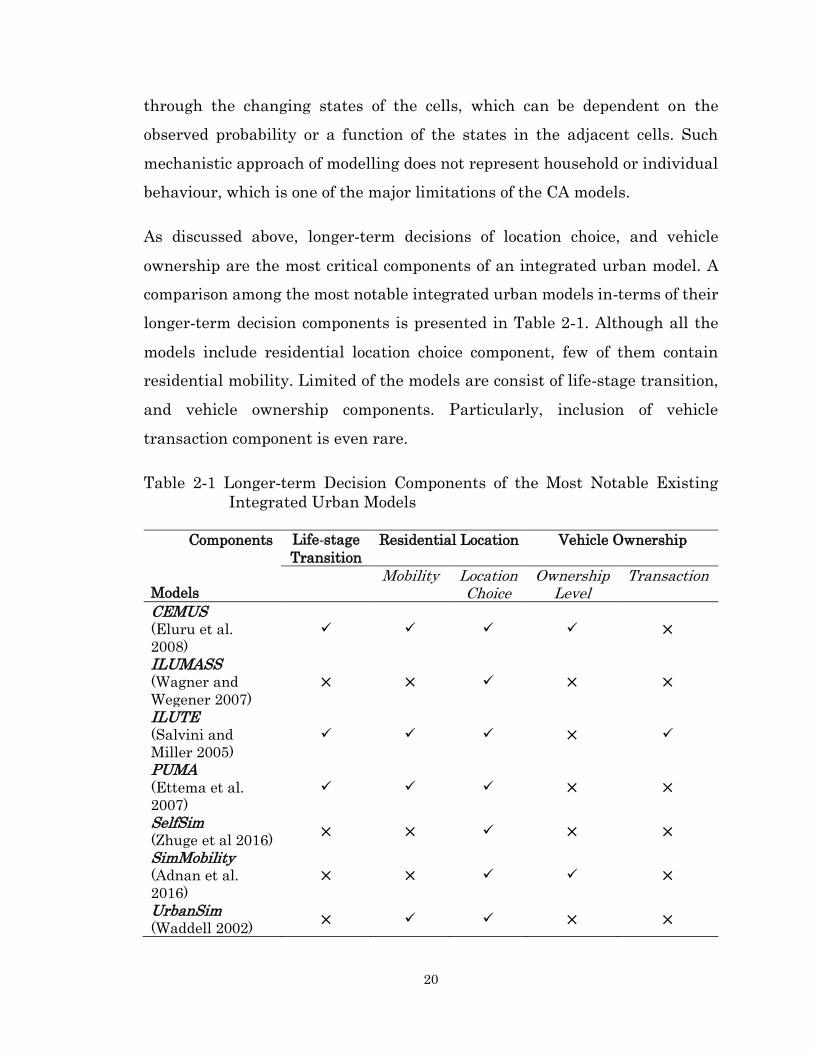
As discussed above, longer-term decisions of location choice, and vehicle
ownership are the most critical components of an integrated urban model. A
comparison among the most notable integrated urban models in-terms of their
longer-term decision components is presented in Table 2-1. Although all the
models include residential location choice component, few of them contain
residential mobility. Limited of the models are consist of life-stage transition,
and vehicle ownership components. Particularly, inclusion of vehicle
transaction component is even rare.
Table 2-1 Longer-term Decision Components of the Most Notable Existing
Integrated Urban Models
Components
Models
Life-stage
Transition
Residential Location Vehicle Ownership
Mobility Location Choice
Ownership Level
Transaction
CEMUS (Eluru et al.
2008)
×
ILUMASS (Wagner and
Wegener 2007) × × × ×
ILUTE (Salvini and
Miller 2005)
×
PUMA (Ettema et al.
2007)
× ×
SelfSim (Zhuge et al 2016)
× × × ×
SimMobility (Adnan et al.
2016) × × ×
UrbanSim (Waddell 2002)
× × ×
21
2.3 Modelling Location Choice, Mode Transition, and
Vehicle Transaction Decisions
Long-term location choice process is the skeletal component of an integrated
urban model, which predicts the spatial configuration of an urban region.
Vehicle ownership is another essential component, since it predicts the vehicle
ownership information of the population that directly feeds into the transport
models to predict the traffic flow as well as test the impacts of strategies
targeting the promotion of sustainable travel choices. Although, generally
commute mode choice is conceptualized as a short-term decision, it has a
longer-term dimension as well. Unless the modelling paradigm of these critical
decision components represent the behaviour adequately, reasonable
understanding and forecasting of the phenomenon might be challenging. A
review of modelling such longer-term decisions is presented in the section
below.
2.3.1 Modelling Residential Location
Residential location decisions have an inherent process orientation in relation
to mobility and determination of location. In the process of relocation,
households first decide to move, then they choose a location. Moreover, the
location component itself is a two-tier process of search and choice of a location.
In this process, households first undertake a search process to identify
potential location alternatives, and finally move to a location. Although a vast
amount of literature exists on modelling location choice decisions, limited
studies have addressed the mobility (Habib and Miller 2008) and search
processes (Rashidi and Mohammadian 2011). Particularly, one of the major
challenges in modelling spatial choice decisions such as residential location is
to address the search process. One approach is to consider all available location
alternatives (e.g., Thill and Horowitz 1991); however, this method is not

22
behaviourally realistic as households do not evaluate all the alternatives
during relocation (Fotheringham 1988). Moreover, the estimation process is
computationally burdensome due to a substantial number of location
alternatives. The most widely used method for reducing computational burden
is to randomly select a subset from the all available alternatives (Ben-Akiva
and Lerman 1985, Guevara 2010). Although the random sampling approach
provides a consistent estimate (McFadden 1978, Guevara and Ben-Akiva
2013), it is merely a statistical method to reduce the number of location
alternatives and ignores behavioural realism of the search process. Another
method is the constrained-based sampling technique, where all the
alternatives within a certain threshold range of a parameter are considered in
the choice set (Zheng and Guo 2008). The underlying deterministic nature of
this technique lacks to capture behavioural realism adequately.
A more plausible approach is to develop behaviourally realistic search model,
where households formulate a pool of potential location alternatives (Habib
and Miller 2007). In this line of research, a number of studies have attempted
to address the search process (Rashidi and Mohammadian 2015, Fatmi et al.
2016). One of the limitations of these studies is to develop the search model on
the basis of single attribute. For instance, Rashidi and Mohammadian (2015)
developed a hazard-based screening model for spatial search based on average
commute distance. Fatmi et al. (2015) considered the influence of prior
locations in generating the potential choice set for the subsequent location on
the basis of distance to the CBD. Advancing the research on residential search,
Bhat (2015) developed a search model that probabilistically generates choice
set using multidimensional housing attributes. One of the most notable
contributions in this paradigm is made by Rashidi et al. (2012), who developed
a hazard-based search model to generate household-specific choice set on the
basis of commute distance and average land value. However, the location
choice model developed using choice set generated from the hazard-based
23
search model did not improve the model fit compared to the random sampling
model (Zolfaghari et al. 2012).
Further, the choice of residential location evolves over the life-time of the
households, as they move from one location to another along the life-course.
Most of the previous researches ignore such dynamics and are static in nature
(Pinjari et al. 2011, Eluru et al. 2010, Gehrke et al. 2014, Lee and Waddell
2010). Few studies have taken a dynamic approach to examine how changes
along the life-time influences location choice. For example, Habib and Miller
(2009) developed a reference dependent mixed logit model to investigate the
role of status quo and response towards gains and losses during location
decisions. Chen and Lin (2011) investigated the effects of historical deposition
on location decisions and argued that the choice of prior locations has an
influence on the choice of the subsequent locations. Strom (2010) tested the
effects of life-cycle events and revealed that the birth of the first child is
associated with the choice of larger-sized dwelling with a higher number of
rooms. Kim et al. (2005) argued that households with young children prefer to
reside in locations on the basis of educational opportunities, residential
facilities, and open spaces. They also revealed that households start to value
job accessibility as children grow older. Recently, some studies have examined
the effects of timing of the life-cycle events on vehicle ownership level (Oakil et
al. 2014), and mode transition decisions (Oakil et al. 2011). It is critical to
address the timing of an event, since households require time to adjust prior
to or after an event in the life-course. Further examination on the life-
trajectory dynamics of residential location choice decisions is necessary.
2.3.2 Modelling Commute Mode Transitions
As residential relocation is a significant decision in the life-time of the
households, a change in location might be directly associated with different

24
decision processes such as mode choice. Mode choice, particularly for commute,
is an important travel decision that has a profound longer-term dimension, as
many change their commute mode over the course of life in response to
changing life circumstances (Oakil et al. 2011). Commuting is the most
frequently made daily trip, as a result individuals become habitual in their
choice of commute mode (Gardner 2009). Since habit persistency is a natural
phenomenon of human behaviour (Bamberg et al. 2010), individuals are
resistant to changes in their commute mode (Kenyon and Lyons 2003).
Commute mode changes are more often the result of key long-term change of
state such as, residential/work location change (Stanbridge et al. 2004, van der
Waerden et al. 2003), change in auto ownership level (Zhang 2006), or
occurrence of life-cycle events, such as household formation, birth of a child, or
residence members moving in or out (Oakil et al. 2011, Verhoeven et al. 2005).
Among the long-term changes, change in residential location considerably
influences a change in commute mode (Dargay and Hanly 2007, Stanbridge et
al. 2004). Stanbridge et al. (2004) demonstrated that a change in residential
location might trigger a change in commute mode choice. Indeed, over one-
quarter (27%) of home movers surveyed changed their commute mode
following relocation (Stanbridge and Lyons 2006). Similarly, Dargay and
Hanly (2007) found that the occurrence of commute mode changes was
associated with residential relocation among the respondents in the British
Household Panel Survey. Clark et al. (2003) developed a probability model to
investigate how one worker and two worker households evaluate commute
distance in choosing their work locations.
The reason for a close association between relocation and mode switch is
attributed by the fact that a change in residential location changes the built
environment, and accessibility characteristics of the home neighbourhood;
which influences the choice of commute mode. For instance, individuals living
in urban areas are more likely to commute by transit/walking/biking, whereas
25
suburban residents tend to be more auto-dependent (Schwanen and
Mokhtarian 2005). Locations with higher mixed land use encourages the use
of transit and active transportation, and discourages the use of car (Cao et al.
2009). Individuals living in urban areas walk more (Coogan et al. 2007) and
choose to take more transit trips (Kitamura et al. 1997). On the other hand,
individuals who prefer single-detached dwellings and single occupancy
vehicles (SOV), live in sub-urban areas (Mae 1997) and own cars (Wachs and
Crawford 1992). Although the relationship between residential location choice
and commute mode choice is evident in the literature, limited studies have
examined how a change in residential location influences a change in commute
mode choice.
Mode transition has been investigated as a longer-term decision by Oakil et al.
(2011), Fatmi and Habib (2017), and as a shorter-term decision by Hess et al.
(2007), among others. Shorter-term mode changes have been examined in
response to temporary incentives (Nurdeen et al. 2007) and acquisition of
specific travel information (Athena et al. 2010). Recently, researchers have
shown interest in analyzing individuals’ mode transition behaviour as a longer-
term decision. For instance, Oakil et al. (2011) developed a panel model to
investigate how individuals’ switch commute mode to and from car. Clark et
al. (2015) developed a logistic regression model to analyze the behaviour of car
commute and transition to and from car, active transportation commute and
transition to and from active transportation. Wang and Chen (2021) developed
a structural equation model of mode switching behaviour between single
occupancy vehicle driving (SOV) and carpooling using data from the Puget
Sound Transportation Panel (PSTP) survey. Idris et al. (2015) used a stated
preference survey to investigate the mode shift behaviour of car drivers. They
focused on the behaviour of continuing with car and shifting from car to transit
and other modes. Although, the importance of understanding mode transition
as a longer-term decision has been identified, a gap nonetheless exists in the
26
literature regarding how mode-specific mode transition occurs along the life-
course of the individuals in response to relocation.
2.3.3 Modelling Vehicle Transactions
Modelling vehicle ownership has emerged from the concern for energy security
and emission reduction. Vehicle ownership is an important medium-term
decision, which interacts with the long-term decisions of where to live, where
to work, as well as short-term decisions of what mode to choose, where to
travel. It is one of the most explored phenomenon in the field of modelling
travel behaviour. A review of literature suggests that a wide-array of
dimensions of the phenomenon is investigated, including vehicle ownership
level (Anowar et al. 2014), vehicle type choice (Garikapati et al. 2014), vehicle
transaction (Mohammadian and Miller 2003), vehicle vintage type (Bhat et al.
2009), and vehicle holding and usage (Bhat and Sen 2006). For example,
Anowar et al. (2014) investigated the vehicle ownership level in four categories:
zero, one, two, and three or more vehicles. Garikapati et al. (2014) estimated a
joint model of vehicle count for the following five vehicle types: car, SUV, van,
pickup, and motorbike. Vehicle transaction was investigated as the transaction
decisions of purchase, disposal, do nothing, and trade of vehicles by
Mohammadian and Miller (2003). Bhat et al. (2009) investigated the choice of
vehicles by the following two categories of vintage types: new vehicles (vehicle
age less or equal to five years), and old vehicles (vehicle age more than five
years). Bhat and Sen (2006) developed a vehicle holding model by examining
households’ usage (annual miles travelled) of different types of vehicles.
Vehicle transaction is a dynamic decision making process which refers to
addition, disposal, and trading of vehicles. Recently, researchers have
attempted to extend the dynamics of the model by accommodating the effects
of life-cycle events on vehicle transaction decisions (Kitamura 2009, Oakil et
27
al. 2014). For example, Yamamoto (2008) investigated vehicle transaction
decisions using longitudinal data from two surveys conducted in France and
Japan. In the case of France, the study developed a competing-risk hazard-
based duration model to examine acquisition, disposal, and replacement
decisions utilizing data from a nationwide panel survey conducted in France.
For Japan, the study developed a multinomial logit model to examine increase,
decrease, and no change in the number of household vehicles using data from
a retrospective component of the person trip survey conducted in Kofu City,
Japan. The study found that life-cycle events, such as residential relocation,
and change in the number of adults in the household significantly affect the
vehicle transaction decisions. Rashidi and Mohammadian (2011) investigated
the interdependencies among residential relocation, employment relocation,
and vehicle transaction utilizing panel data from the Puget Sound
Transportation Study conducted in the Seattle Metropolitan Area, U.S.A. They
formulated a hazard-based system of equations, where residential and
employment relocations are included as endogenous variables in the vehicle
transaction model to predict the timing of vehicle ownership change. They
found that a change in job is more likely to influence a household to make a
vehicle transaction; whereas, a residential relocation was found to show a
lower likelihood to change the household vehicle fleet size. In this line of
research, Oakil et al. (2014) further tested the effects of timing of life-cycle
events on vehicle transactions. They developed a mixed logit model to
investigate vehicle transaction decisions; particularly, focusing on the vehicle
acquisition and disposal decisions. The study revealed that households require
adjustment period before and after a life-cycle event. For example, households
were found to purchase a vehicle in anticipation of the child birth and dispose
of a vehicle after changing a job. However, further investigation is required
regarding developing dynamic models for vehicle transaction decisions.

28
2.4 Issues in the Existing Integrated Urban Models
In summary, long-term, medium-term, and short-term decisions are essential
components of IUMs. There is an inherent inter-dependency among these
decisions. For example, long-term decision of where to live influences medium-
term and short-term decisions of whether or not to own a vehicle, what mode
to choose, and vice versa. Integrated urban models need to be responsive to
these decision dynamics across the agents’ life-stages; starting with residential
location, vehicle transaction, and life-stage transitions. However, such multi-
way feedback mechanism is not well addressed within the existing urban
modelling framework.
It is also required to examine how a change in critical long-term state such as
residential location triggers a change in decisions of other life-domains such as
commute mode choice. In the existing literature, dynamic modelling of
commute mode transition decisions associated with the changes in residential
location over the life-time of the individuals have not occurred to any
significant extent. Moreover, limited studies have considered mode-specific
mode transition among a comprehensive set of modes, such as car, transit, and
active transportation (walk/bike).
An important aspect is addressing the process orientation of the essential
decisions, which is limited in the existing urban modelling literature. For
example, residential location is a two-stage process of mobility and location
choice. Majority of the integrated models focuses on the location choice
decision. Only a few, such as ILUTE, CEMUS, UrbanSim, and ILUMASS have
the mobility component. However, to avoid complexity during implementation,
some of the models, for example, UrbanSim and ILUMASS use historical rates
in-place of behavioural models for the mobility module. Even the location
choice component can be characterized as a two-tier process of home search
and location choice. In the modelling paradigm of residential location, some
29
attempts have been made to address the search process. Such efforts have not
warranted improvements in the empirical estimation of location choice models
(Zolfaghari et al. 2012). Further examination is necessary on how to address
the process orientation of the decisions; particularly, the long-term and
medium decisions of residential location and vehicle transaction.
Although vehicle ownership is an important element for both the land use and
transport components of the IUMs, few of the existing IUMs such as ILUTE,
CEMUS, and SimMobility have this module. Only ILUTE accommodates
vehicle transaction simulation, including acquisition, disposal, and trade.
However, acquisition of a vehicle has an underlying dimension of whether the
household is purchasing the first vehicle in their lifetime or the household is
adding a vehicle to the already existing vehicle fleet. It is critical to identify
the transaction decision of the first time vehicle purchase, since purchasing the
first vehicle is a key event itself in the lifetime of the household which might
trigger a mode shift to car. Therefore, in addition to implementing the vehicle
transaction, such extension towards first vehicle purchase is necessary.
To address the life-trajectory dynamics of different decision processes within
the IUM framework, individuals’ life-stages have to be simulated. A large body
of literature exists on the population demographic microsimulation (Nelissen
1993, Gribble 2000, Orcutt et al. 1976, King et al. 1999); however, integrated
urban models have not sufficiently addressed life-stage transition processes.
In addition, one of the major purposes of integrated urban models is to predict
the evolution of urban form. Limited of the existing models are operational to
report the spatio-temporal evolution of an urban region at the disaggregate-
level of individuals as well as at the micro-spatial resolution.
In terms of modelling techniques, innovative methods need to be developed
that accommodate the life-trajectory dynamics such as the process orientation
of the decisions, and hold the potential to improve the empirical estimation

30
procedure. Models are also required to capture the multi-way decision
dynamics; particularly, interactions among longer-term decisions of residential
location, vehicle transaction, and life-stage transitions. These decisions are
significant events in the life-time of the households, which require considerable
investment of time and money. Hence, households might need adjustment
period prior to or after an event/decision in the life-course. It is important to
accommodate such time dimension of decisions and life-cycle events within the
model estimation technique. Another temporal dimension is the repeated
choices made by the same households along their life-course when panel
observations are considered. For instance, in the case of residential location,
households repeatedly move from one location to another along their housing
career. Due to the repeated location choices, there exists a correlated sequence
of choices, which demands accommodation within the empirical formulation of
the models. Furthermore, models should address the heterogeneity among the
households/individuals during the decision making processes.
Although considerable progress has been made in developing integrated urban
models based on fundamental theories and approaches, such as economic
activity-based models, market principle models, quasi market-based models,
hybrid models, and agent-based complex system models; however, life-oriented
approach is rarely adopted in developing urban models. A life-oriented
perspective and theory is required to address the life-trajectory dynamics of
key household-level decision processes, such as residential location and vehicle
transaction. Life-oriented approach focuses on how transitions along the life-
time and interactions among decisions taken at different life-domains shape
individuals’ choices and behaviour (Chatterjee Scheiner, 2015, Zhang 2017,
Zhang 2015). Life-oriented approach and perspective offers the opportunity to
disentangle a wide-ranging modelling issues such as multi-domain decision
interactions, evolution of life-stages of individuals and households, evolving
31
nature of the decisions along the life-course, and process orientation of the
decisions, among others.
2.5 Research Questions and Concluding Remarks
From the above discussion, it is evident that a wide-ranging theories,
modelling methodologies, and simulation frameworks are developed to address
the evolution of urban systems through integrated urban modelling. However,
representing greater behaviour of the agents during longer-term decision
processes as well as adding the capacity to reasonably predict the spatio-
temporal evolution of the urban region demand further investigation.
Particularly, the following research questions need to be addressed:
1. How to accommodate life-trajectory dynamics within key household-
level longer-term decision models?
2. How to represent process orientation within the micro-modelling
structure as well as computational procedure of an integrated urban
model?
3. How to advance development of integrated urban systems model taking
a life-course perspective and predict the micro-level evolution of the
urban region?
This research attempts to address the above mentioned research questions.
Specifically, this study adopts a life history-oriented approach to develop an
agent-based integrated urban model that encompasses the modelling and
simulation of longer-term decision processes, including life-stage transitions,
residential location, first time vehicle purchase, and vehicle transaction.
Interactions among these decisions are established within the empirical and
computational procedures. The process orientation of the agents’ decisions are
accommodated during developing the modelling methodologies, which is later
translated to the simulation framework. Further in the modelling paradigm,
32
this study investigates how a change in commute mode is associated with a
change in residential location. Innovative modelling techniques are developed
to accommodate the life-trajectory dynamics of the decision processes. The
proto-type integrated urban model developed in this study is capable of
predicting the micro-level spatio-temporal evolution of the population in an
urban region.
33
Chapter 3
3 Conceptual Framework and Data
3.1 Theoretical Context
The need to recognize the multi-directional interactions among the household
decision processes has motivated this research to develop a life-oriented
integrated Transport Land Use and Energy (iTLE) Model. The proposed model
is developed on the basis of solid theoretical foundation, and includes a
comprehensive set of decision components. To address the multi-way
interactions and temporal dimension, the software architecture including the
micro-modelling structures and computational procedures consistently adopts
the concept of life-oriented approaches and theories. Life-oriented approach
focuses on the inter-dependencies among the decisions and changes occurring
at different life-domains of people (Zhang 2017, Zhang 2015). Zhang et al.
(2011) identified nine major life-domains, such as residence, job, education and
learning, health, family life, family budgets, neighbourhood, leisure and
recreation, and travel behaviour; and revealed that interactions exist among
the decisions taken in different life-domains (Zhang 2014). To develop better
empirical and simulation models of household-level decision processes, it is
imperative to examine the interactions among changes in multiple life-
domains, since choices at any domain are part of the extended inter-connected
choices made hierarchically across different domains (Salomono and Ben-
Akiva 1983, Lanzendorf 2003).
A life-oriented approach could take a life-course perspective, also known as life
history-oriented approach. Life history-oriented approach focuses on the
temporal variation of the multi-domain interactions over the life-course.
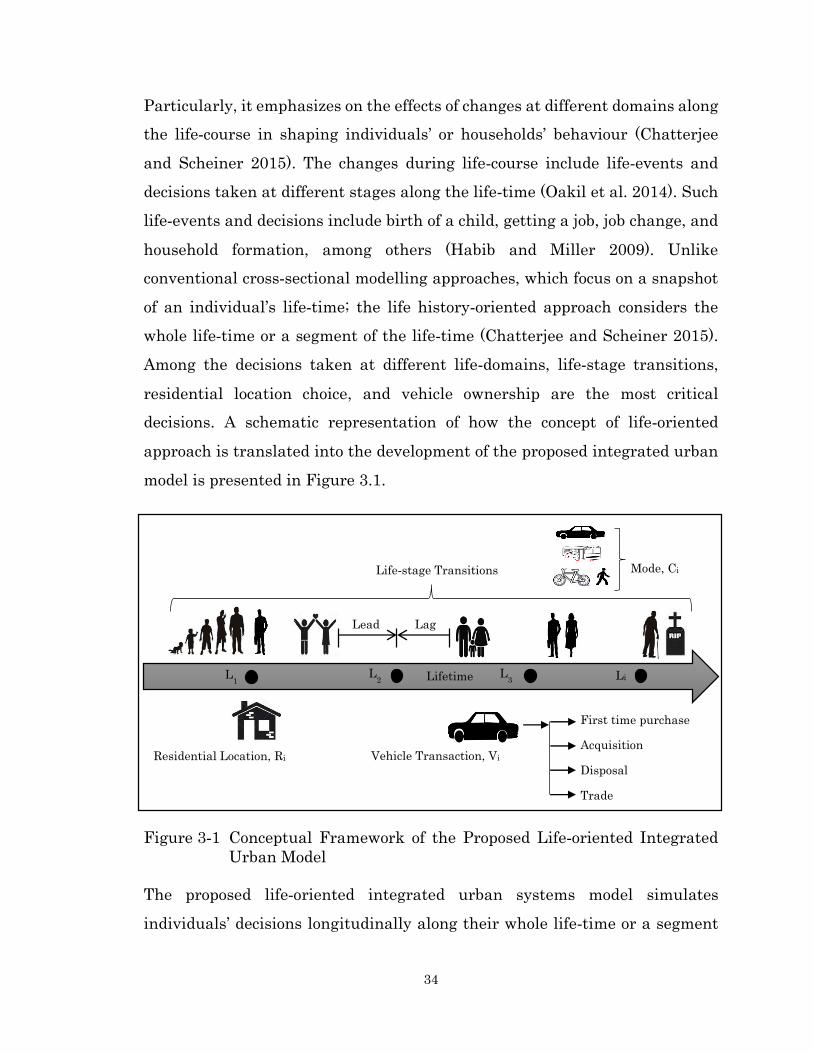
34
Particularly, it emphasizes on the effects of changes at different domains along
the life-course in shaping individuals’ or households’ behaviour (Chatterjee
and Scheiner 2015). The changes during life-course include life-events and
decisions taken at different stages along the life-time (Oakil et al. 2014). Such
life-events and decisions include birth of a child, getting a job, job change, and
household formation, among others (Habib and Miller 2009). Unlike
conventional cross-sectional modelling approaches, which focus on a snapshot
of an individual’s life-time; the life history-oriented approach considers the
whole life-time or a segment of the life-time (Chatterjee and Scheiner 2015).
Among the decisions taken at different life-domains, life-stage transitions,
residential location choice, and vehicle ownership are the most critical
decisions. A schematic representation of how the concept of life-oriented
approach is translated into the development of the proposed integrated urban
model is presented in Figure 3.1.
Figure 3-1 Conceptual Framework of the Proposed Life-oriented Integrated
Urban Model
The proposed life-oriented integrated urban systems model simulates
individuals’ decisions longitudinally along their whole life-time or a segment
Lifetime
L2 L
3
Lead
event
Lag
even
t
Mode, Ci
Li
Residential Location, Ri
L
1
Vehicle Transaction, Vi
First time purchase
Acquisition
Disposal
Trade
Life-stage Transitions
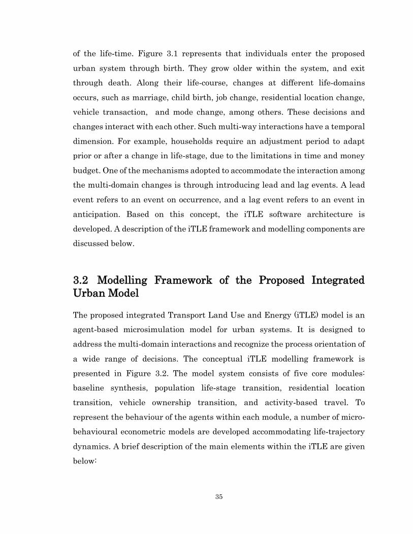
35
of the life-time. Figure 3.1 represents that individuals enter the proposed
urban system through birth. They grow older within the system, and exit
through death. Along their life-course, changes at different life-domains
occurs, such as marriage, child birth, job change, residential location change,
vehicle transaction, and mode change, among others. These decisions and
changes interact with each other. Such multi-way interactions have a temporal
dimension. For example, households require an adjustment period to adapt
prior or after a change in life-stage, due to the limitations in time and money
budget. One of the mechanisms adopted to accommodate the interaction among
the multi-domain changes is through introducing lead and lag events. A lead
event refers to an event on occurrence, and a lag event refers to an event in
anticipation. Based on this concept, the iTLE software architecture is
developed. A description of the iTLE framework and modelling components are
discussed below.
3.2 Modelling Framework of the Proposed Integrated
Urban Model
The proposed integrated Transport Land Use and Energy (iTLE) model is an
agent-based microsimulation model for urban systems. It is designed to
address the multi-domain interactions and recognize the process orientation of
a wide range of decisions. The conceptual iTLE modelling framework is
presented in Figure 3.2. The model system consists of five core modules:
baseline synthesis, population life-stage transition, residential location
transition, vehicle ownership transition, and activity-based travel. To
represent the behaviour of the agents within each module, a number of micro-
behavioural econometric models are developed accommodating life-trajectory
dynamics. A brief description of the main elements within the iTLE are given
below:
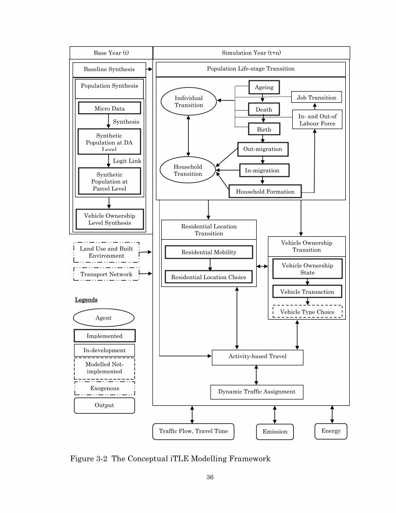
36
Figure 3-2 The Conceptual iTLE Modelling Framework
Death
Birth
Synthetic
Population at
Parcel Level
Synthetic
Population at DA
Level Out-migration
Household
Transition
Individual
Transition Micro Data
Baseline Synthesis
Residential Location
Transition
Residential Mobility
Residential Location Choice
Vehicle Ownership
Transition
Vehicle Ownership
State
Vehicle Type Choice
Vehicle Transaction
Dynamic Traffic Assignment
Activity-based Travel
Traffic Flow, Travel Time Energy Emission
Synthesis
Population Life-stage Transition
Implemented
Modelled Not-
implemented
In-development
Exogenous
Output
Agent
Update
Legends
Household Formation
In-migration
In- and Out-of
Labour Force
Job Transition
Logit Link
Vehicle Ownership
Level Synthesis
Population Synthesis
Base Year (t) Simulation Year (t+n)
Land Use and Built
Environment
Transport Network
Ageing
37
3.2.1 Baseline Synthesis
The baseline synthesis component generates micro-level information of the
population for an entire urban region, which is used as an input for the
microsimulation engine of iTLE. The baseline synthesis involves population
synthesis and vehicle ownership level synthesis for the initial time-step.
Population synthesis for the iTLE is performed as a two-stage process. First, a
synthetic population is generated controlling for both household-level and
individual-level characteristics at the smallest zonal level of dissemination
area (DA). In the second stage, households are allocated into the micro-spatial
unit of parcel. In addition, relevant baseline information, for instance, vehicle
ownership level for the synthetic population is generated.
3.2.2 Population Life-stage Transition
Population life-stage transition module focuses on the evolution of the
demographic career of the agents. Relevant life-stage transitions along the life-
course of the individuals and households are simulated. This process includes
simulation of eight transitions: ageing, death, birth, out-migration, in-
migration, household formation, in- and out-of labour force, and job transition.
3.2.3 Residential Location Transition
Residential location transition module follows the theory of residential stress
(Rossi 1955), which postulates that households decision to move or stay at a
location is triggered by the residential stress developed at that location. Stress
is generated by the experienced or desired changes in life-stages (Miller 2005),
dwelling characteristics (Van Ham and Feijten 2008), and neighbourhood
attributes (Van Ham and Clark 2009), among others. Such stress arises from
38
the discrepancies between the desired and current situation of a household. As
a result, households’ relocate to a new location that minimizes the stress.
Residential location transition is conceptualized as a two-stage process:
residential mobility, and residential location choice. In the first stage of
mobility, households are assigned to move or stay at a particular location.
Households who are assigned to move in this stage, are considered in the
second stage. The second stage of location choice is assumed as a two-tier
process of location search and choice. In this stage, households first search for
locations, and then choose a location. The search process is conceptualized as
a stress releasing mechanism, where households generate a pool of location
alternatives, which has the potential to minimize the stress. Finally,
households are allocated to one of the locations from the pool of alternative
locations. In addition, the location transition module includes a commute mode
transition component. Following a relocation, individuals are conceptualized
to reassess their commute mode. After reassessing, individuals either continue
with the same mode, or make a transition to a new mode. A description of the
micro-behavioural models and microsimulation results of the residential
location transition process are presented in Chapter 4 and Chapter 6
respectively.
3.2.4 Vehicle Ownership Transition
Vehicle ownership transition module is conceptualized as a three stage process:
vehicle ownership state, vehicle transaction, and vehicle type choice. The first
stage of vehicle ownership state has two components: no vehicle ownership
state, and transient ownership state, as conceptualized by Khan and Habib
(2016). Households not having a transaction history in their lifetime are
assumed to be in the no vehicle ownership state. Households having a
transaction history in their lifetime are assumed to be in the transient

39
ownership state. The second stage of vehicle transaction focuses on the
transaction decisions of the households. This component involves the following
four transaction elements: first time vehicle purchase, acquisition, disposal,
and trade. In the third stage, vehicle type choice behaviour is simulated for the
households making the decisions of first vehicle purchase, acquisition, and
trade in the earlier stage. In this stage, the simulation determines the choice
among six vehicle types: sub-compact, compact, mid-size, luxury, SUV, and
van. The micro-behavioural models and microsimulation results for the vehicle
transaction component is reported in Chapter 5 and Chapter 7 respectively.
The vehicle type choice model is developed by Khan and Habib (2016), and will
be implemented later.
3.2.5 Activity-based Travel
This module simulates the travel activities of the individuals, following an
activity-based modelling technique. Microsimulation of activity generation,
scheduling, and mode choice behaviour are included in this module. Finally,
the travel patterns/trips of the individuals are simulated on the transport
network using a dynamic traffic assignment method. This module is currently
under development, and beyond the scope of this study.
3.2.6 Population and Urban Form Representation
The efficiency and accuracy of an urban systems simulation model largely
relies on how closely it replicates individuals’ behaviour, and relationships
with built environment. In terms of representing individuals’ behaviour, agent-
based microsimulation modelling is necessary to effectively abstract a complex
and dynamic system like an urban region. Therefore, the iTLE represents
population at the most disaggregate-level, assuming individuals and
households as the agents.

40
Urban form is represented at the most micro geographic unit of parcel, since
residential location component is conceptualized to be modelled considering
parcels as the spatial unit of analysis. The micro-scale spatial resolution
improves the capability of the model to represent better individual behaviour
and effectively analyze micro-scale land use policies. Each parcel acts as a
property object, which is characterized by its location (centroid of a parcel),
size, type, and accessibility to major activity points and service destinations.
The parcel database also maintains the characteristics of more aggregate
spatial information, such as dissemination area (DA) based on its location.
Maintaining the relationship between parcels and corresponding DAs assists
in generating numerous statistics and maps at different aggregation levels for
further analysis of the simulation results.
3.3 Data Sources and Description
Development of a life-oriented agent-based microsimulation model for urban
system like iTLE requires a tremendous amount of data. Particularly, the focus
of iTLE is to address interactions among different decisions along the life-
course of the agents as well as process orientation of the decisions. To
accommodate such dynamics within the empirical settings, data from
conventional cross-sectional surveys are not adequate. Longitudinal survey
data are required, which provides information about the life history of
respondents. Therefore, this research utilizes retrospective survey data to
develop the micro-behavioural components of the iTLE model. A description of
the retrospective survey data is presented below.
3.3.1 Retrospective Survey Data
The data source for developing the micro-behavioural models is a retrospective
Household Mobility and Travel Survey (HMTS). The HMTS was administered
41
from September 2012 to April 2013 in Halifax (Peterlin and Habib 2013,
Heffernan and Habib 2013). The design of the HMTS was in accordance with
previous retrospective surveys, including Residential Mobility Survey I and II
(Haroun and Miller 2004), and Residential Search Survey, which were
conducted in Toronto, Canada (Habib and Miller 2009). The HMTS collected
life-history information across the life-domains of the households, including
housing history, vehicle ownership history, compositional change, and
employment record, among others. A brief description of these components are
given below:
1. Housing history: The housing history component collected information
regarding the three most recent residential episodes of the respondents.
For each residential episode, respondents were asked to provide the
following information:
Location information including civic address and postal code.
Year and month of relocation.
Primary reasons for relocation. The reasons are thematically
aggregated into the following four major categories: (1) to live in
proximity to work or key activity locations, such as school, shopping
center, entertainment, and transit stop; (2) to live in desirable
neighbourhood or dwelling; (3) due to life-cycle events such as change
in household size and formation of a new household; and (4) other
reasons.
Socio-economic and demographic configuration of the household,
including household income, household size, number of children,
number of vehicles, number of driver’s licence, number of bicycles,
and monthly transit pass ownership, among others.
Dwelling characteristics, which includes dwelling type, tenure type,
number of rooms, and number of bedrooms, among others.
42
Choice of primary commute mode, which can be broadly categorized
into the following options: car, transit, and active transportation
(walk/bike).
2. Vehicle ownership history: This component collected information
regarding households’ vehicle ownership history up to four current and
four previous vehicle ownerships. The following information of the
vehicles are collected: make, model, manufacturing year, purchase year,
new or used, purchased or leased, and purchase price, among others.
3. Household compositional change: Household compositional change
refers to the change in size of the household and number of employed
household members. This component includes the following
information:
Year of a change in the household size as a result of birth, death, a
member moving out, or a new member moving in.
Year of a change in the employment size as a result of addition of a
job, loss of a job, retirement, withdrawal from the labour force, or a
return to school.
4. Employment records: The employment career component collected
information of the three most recent employments, including
employment location, employment type, employment starting and
ending year and month.
5. Attitudinal and other information: The survey contained 33 statements
concerning attitudes. The respondents were asked attitudinal questions
on a three point agree-disagree likert scale to specify their level of
43
agreement or disagreement. In addition, travel time and travel mode of
a number of major travel activities are collected.
The HMTS provided a total response from 475 households. The proportion of
men and women in the sample is almost equal. In the case of age distribution,
54% of the respondents’ age are below 35 years, and 16% of the respondents
are above 54 years. 33% respondents earn a household income of above
$100,000 (CAD), and 31% earn a household income of below $50,000 (CAD).
Around 38% of the respondents represent two-person households, and 9%
represent five or more person households. Around 50% of the respondents
reside within the regional centers, and 38% lives in suburban areas. The
HMTS sample was compared with the Statistics Canada Census for Halifax
Regional Municipality (HRM) by Salloum and Habib (2015). They found that
majority of the stratums of household and individual characteristics are within
a 3% variability of the 2011 Census information. Hence, the HMTS can be
considered as a representative sample. Further detail of the validation and
exploratory analysis of the survey can be found in Salloum and Habib (2015).
3.3.2 Secondary Data Sources
This study utilizes information from a number of secondary data sources
during the model estimation and simulation procedures. A list of these
secondary data sources are presented in Table 3-1. A brief description of the
data is presented below.

44
Table 3-1 List of Secondary Data Sources Utilized to Develop the
Components of the Proposed Integrated Urban Model
Data Items Data Sources Data Descriptions Model Components
Micro sample of
the population
PUMF Individual- and household-level
socio-economic characteristics of
a random micro sample
Zonal-level
Population
Synthesis
Target total of
the population
at the zonal level
of DA
Census Distribution of the population
falling under different categories
of socio-economic characteristics
at the DA-level
Zonal-level
Population
Synthesis,
Validation
Parcel
information
Nova Scotia
Property
Database
Parcel location, size, and type Logit link, Search,
Location Choice
Historical rates Census Historical rates of different
demographic events
Life-stage
Transition
Activity point
location
DMTI** Location of schools, central
business district (CBD), business
parks, health services, park
areas, and shopping centers
MM*
Transport
service location
DMTI** Location of bus stops MM*
Neighbourhood
characteristics
Census Socio-economic and demographic
characteristics at the DA-level
MM*
DA boundaries Census DA boundary file in the GIS
platform
Zonal-level
Population
Synthesis and MM*
Road network HRM*** Road network layer in the GIS
platform
MM*
Land use
information
HRM*** Polygon file of different land uses
at the DA-level in the GIS
platform
MM*
*MM refers to all developed micro-models of the iTLE system, which includes residential mobility, search,
location choice, mode transition, vehicle transaction, logit link, and vehicle ownership level synthesis.
**DMTI refers to Desktop Mapping Technologies Inc.
***HRM refers to Halifax Regional Municipality
45
3.3.2.1 Census Data
The data used for generating the population synthesis includes: 2006 Public
Use Microdata File (PUMF), and 2006 Census information at the
dissemination area (DA) level. The PUMF data is used as the micro sample
and the Census data is used as the control total for the population synthesis.
The 2006 PUMF data includes micro-level information of the population in
Atlantic Canada. The sample size is 20,954 individuals and 8,907 households.
The sample size of the 2006 Census data for Halifax is 372,679 individuals and
155,060 households. The spatial resolution of the collected census data is at
the smallest zonal-level of dissemination area (DA). The Halifax region
includes a total of 572 DAs. For validation purposes of the iTLE, 2011 Census
information are collected. The 2011 Census includes 390,325 individuals,
165,155 households, and 594 DAs. This data is also utilized to represent the
neighbourhood characteristics at the DA-level.
3.3.2.2 Land Use Data
To represent the urban form, parcel-level data is collected from the Nova Scotia
Property Database 2013. This parcel database provides information regarding
parcel attributes, including location, size, and type, among others, of all the
parcels in the Province of Nova Scotia. Following the cleaning process, a total
of 110,995 parcels for Halifax are derived. Additional data sources include
location of different activity points, such as location of schools, central business
district (CBD), business parks, health services, park areas, and shopping
centers; which are collected from the Desktop Mapping Technologies Inc.
(DMTI). Location of transportation services such as transit stop locations are
collected from the DMTI. Land use data referring to the percentage of different
land uses at the DA level are collected from the Halifax Regional Municipality
(HRM). Road network is collected from the HRM as well.
46
3.4 Derived Independent Variables
The micro-behavioural models for residential location, vehicle transaction, and
mode transition, developed in this study, accommodate the effects of a wide
range of independent variables, such as, life-cycle events, socio-demographics,
dwelling characteristics, parcel characteristics, accessibility measures, and
neighbourhood characteristics, among others. A brief description of the
variables derived from the above discussed data sources are presented below.
3.4.1 Life-cycle Events
One of the unique features of this study is to develop micro-models that are
capable of exploring the priori hypotheses regarding the interactions among
multi-domain longer-term changes. These longer-term changes along the life-
course of the individuals and households are termed as life-cycle events. Life-
cycle events include, birth of a child, death of a member, move-in of a member,
move-out of a member, household formation, residential relocation, addition of
a job, loss of a job, job change, retirement, and vehicle transaction, among
others. Vehicle transaction decision includes the decision of vehicle acquisition
and purchase of the first vehicle. “Vehicle acquisition” refers to the addition of
a vehicle to the existing vehicle fleet of the household. “Purchase of the first
vehicle” refers to the purchase of the first vehicle in the life-time of the
household. “Job change” is defined as getting a job following the loss of a job
within the same month of the same year. “Addition of a job” refers to getting
the first job or getting a new job after one month of losing the previous job.
“Loss of a job” refers to losing a job and failing to secure another job within the
same month. Households require adjustment period before/after a life-cycle
event. The adjustment period is accommodated within the models by
considering the events as lead and lag events. Lead events refer to the effects
of an event on occurrence, and lag events refer to the effects of an event in

47
anticipation. Hence, a lead event indicates to a lagged effect, and a lag event
indicates to a lead effect. The micro-models consider lead and lag events for the
following periods: same year, one-year lead, two-year lead, three-year lead,
one-year lag, two-year lag, and three-year lag. “Same-year” refers that two
events occurred in the same calendar year. “1 year lead” refers that an event
occurred one to two calendar years before another event. Two-year lead and
three-year lead can be described similarly. “One-year lag” indicates that an
event occurred one to two calendar years after another event. Similarly, two-
year lag and three-year lag can be described. The variables representing life-
cycle events are derived from the HMTS data.
3.4.2 Accessibility Measures
Accessibility characteristics refer to the distance from home location to
different activity points. The location of activity points and transportation
services are utilized to determine the accessibility measures. The accessibility
measures are generated on the basis of the road network distances using the
Network Analyst tool in ArcGIS. The accessibility measures include commute
distance, distance to the CBD, and closest distance to the following locations:
transit stop, business center, school, health service, park area, and shopping
center, among others.
3.4.3 Land Use and Neighbourhood Characteristics
Land use information refers percentages of different land uses measured using
the ArcGIS platform at the DA-level. The data includes land use measures in
the following categories: residential, commercial, open space, park, industrial,
government, and water body. The land-use information is utilized to determine
land-use mix index, which follows the measures proposed in Bhat and Gossen
48
(2004)1. The index value ranges from 0 to 1, where a value of 0 indicates perfect
homogeneity and 1 indicates perfect heterogeneity. Micro-level land use
characteristics, such as parcel size information is derived for estimating the
location choice model. In addition, neighbourhoood characteristics are derived
at the DA-level, which include population density, dwelling density,
percentage of owned dwellings, percentage of rented dwellings, percentage of
single-detached dwellings, average property value, labour force participation
rate, employment rate, percentage of household share of shelter cost to income
less than 30%, and percentage of non-movers, among others.
3.4.4 Socio-demographic and Dwelling Characteristics
The models test a number of socio-demographic characteristics, such as gender,
age, and education level of the head of the household, household size,
household income, presence of children, and number of vehicle ownership.
Dwelling characteristics include, number of rooms in the dwelling unit,
dwelling type, and tenure type, among others.
3.5 Conclusions
This chapter proposes the development of a life-oriented agent-based
integrated urban modelling system, and discusses the conceptual framework
and data utilized to address the multi-dimensional interactions among
different decision processes within the proposed urban systems model. The
theoretical context of the proposed model is discussed in this chapter.
Particular emphasis is given on how life-oriented theory and perspective is
1 Land − use mix index = 1 − {|𝑅
𝑇−
1
3|+|
𝐶
𝑇−
1
3|+|
𝑂
𝑇−
1
3|
4
3
}, where, R = residential land use, C = commercial or
industrial land use, O = other land use, and T = total land use. All land use measures are in acres.
49
mapped within an integrated modelling framework. Conceptualizing on this
approach, the essential components of an urban model are identified, which
includes: baseline synthesis, population life-stage transition, residential
location transition, and vehicle ownership transition. To develop a
comprehensive multi-domain feedback-based microsimulation model, the
requirement for a tremendous amount of data is discussed. Data is collected
from a number of sources and through undertaking specialized surveys. The
primary data source to develop the micro-behavioural models for different core
components of the iTLE is a retrospective survey, known as the HMTS. To
develop the population synthesis module, PUMF and Census data are used.
Description of these data are provided in this chapter. Finally, priori
hypotheses are presented by discussing the independent variables considered
to develop the micro-models. The mechanism to test multi-way interaction
through lead and lag effects of a number of life-cycle events are described. The
next two chapters (Chapter 4 and 5) presents the empirical estimation results
of residential location transition, mode transition, and vehicle transaction
components. The results of baseline synthesis and population life-stage
transition module are presented in Chapter 6. The microsimulation results of
residential location and vehicle transaction are reported in Chapter 7 and 8,
respectively.
50
Chapter 4
4 Modelling Residential Location
Processes
4.1 Introduction
This chapter focuses on modelling the residential location transition processes
of the iTLE model. This study also investigates how a change in residential
location influences a change in commute mode choice. This research
disentangles the following key issues in modelling location choice: 1)
accommodating the process orientation of the phenomenon by modelling
location decision as a two-stage process of mobility and location choice, 2)
addressing the location search process during modelling location choice and
examining whether the incorporation of search process improves the empirical
estimation of the location choice, 3) investigating the effects of multi-domain
decision interactions through introducing life-cycle events as lead and lag
events, and 4) testing how a long-term change such as residential relocation
influences individuals to reassess their commute mode.
As discussed earlier, the residential location process adopts the theory of
residential stress (Rossi 1955). Households’ are conceptualized to relocate due
to the continual generation of residential stress along their life-time.
This chapter is largely derived from the following journal papers:
Fatmi, M.R., Chowdhury, S., and Habib, M.A. (2017). Life History-Oriented
Residential Location Choice Model: A Stress-Based Two-Tier Panel Modelling
Approach. Transportation Research Part A: Policy and Practice, 104, 293-307. Fatmi, M.R., and Habib, M.A. (2015). Spatial Transferability of a Micro Residential
Mobility Model in the Integrated Land Use, Transportation and Environment
Modelling System. Transportation Research Record: Journal of Transportation Research Board, 2494(2), 29-36.
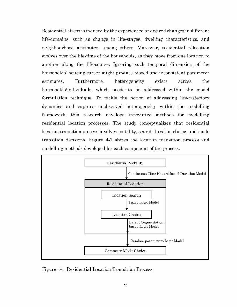
51
Residential stress is induced by the experienced or desired changes in different
life-domains, such as change in life-stages, dwelling characteristics, and
neighbourhood attributes, among others. Moreover, residential relocation
evolves over the life-time of the households, as they move from one location to
another along the life-course. Ignoring such temporal dimension of the
households’ housing career might produce biased and inconsistent parameter
estimates. Furthermore, heterogeneity exists across the
households/individuals, which needs to be addressed within the model
formulation technique. To tackle the notion of addressing life-trajectory
dynamics and capture unobserved heterogeneity within the modelling
framework, this research develops innovative methods for modelling
residential location processes. The study conceptualizes that residential
location transition process involves mobility, search, location choice, and mode
transition decisions. Figure 4-1 shows the location transition process and
modelling methods developed for each component of the process.
Figure 4-1 Residential Location Transition Process
Residential Mobility
Location Choice
Commute Mode Choice
Continuous Time Hazard-based Duration Model
Fuzzy Logic Model
Latent Segmentation-
based Logit Model
Random-parameters Logit Model
Location Search
Residential Location
52
Residential mobility decision is modelled utilizing a continuous time hazard-
based duration modelling technique. Duration refers to the length of stay at a
particular location. Traditional single-episode duration model is extended to a
multiple episode shared frailty framework to accommodate the effects of
repeated durations along the housing career of the households. Both sets of
models are estimated for a number of distributions including lognormal, log
logistic, and Weibull. In the case of residential search, the model is developed
using a fuzzy logic-based modelling method. The model conceptualizes on the
theory of residential stress, and accommodates the inter-dependencies between
push and pull factors. Constraints regarding households’ affordability are imposed
by introducing household income and property value within the fuzzy framework.
The location choice model is developed utilizing a latent segmentation-based logit
(LSL) modelling technique. The LSL model accommodates correlated sequence of
repeated choices through introducing joint probability of choice sequence.
Unobserved heterogeneity in the decision making process is captured by
formulating a flexible latent segment allocation model within the LSL framework.
Finally, the commute mode transition model adopts a random-parameters logit
(RPL) modelling technique. Similar to the LSL framework, the RPL model
formulation accommodates the joint probability of choice sequence. The model
captures unobserved heterogeneity by allowing parameters to vary across the
individuals.
The organization of the rest of the chapter is as follows: section 4.2 discusses
the modelling of residential mobility, particularly, the mathematical
formulation of the model and discussion of the parameter estimation results.
Section 4.3 describes the methods and results of the location search and
location choice model. Section 4.4 presents discussion on the mode transition
behaviour, including the mathematical model formulation and estimation
results. Finally, section 4.5 concludes with a summary of contributions.
53
4.2 Residential Mobility
The first stage of residential location decision is mobility, which refers to the
decision to move or stay at a particular location. The mobility model is
developed utilizing a continuous time hazard-based duration modelling
technique. Duration modelling is widely used in medical sciences, economics
and urban economics (Haurin and Gill 2002, Jenkins and García-Serrano
2004); for example, analyzing the duration of unemployment (Jenkins and
García-Serrano 2004). However, in the residential mobility literature, few
studies have adopted this approach (Decoster et al. 2005, Habib and Miller
2008). This method offers the opportunity to test the influence of life-stages,
dwelling characteristics, land use, accessibility, and neighbourhood
characteristics on the length of stay at a particular location. To address the
life-trajectory dynamics, a household’s housing career is characterized as the
sequence of duration (i.e. episodes/spells) in different dwellings during their
lifetime. The conventional duration model is extended to a multiple episode
shared frailty model. This research also examines whether the multiple
episode shared frailty extension of the model improves the model fit or not.
4.2.1 Methodology
The residential mobility model is developed utilizing a continuous time hazard-
based duration modelling technique. In the formulation of the hazard-based
duration model, duration is specified as the period that a household will
remain in a specific residence and the failure (termination) event is a move to
a different location. Hence, the hazard model considers duration at a particular
residential location as the dependent variable. The data for the model is
extracted from the HMTS survey that contains 475 households with 762
episodes representing duration at a particular residential location, including
censored spells. The data is right censored in April, 2013. The average duration

54
is 2170.924 days (5.96 years) with a minimum of 23 days and a maximum of
15462 days (42.45 years). The duration spells are considered to be continuous
time-periods. This model examines time constant covariates only, meaning
covariates that are constant or can be assumed to be time-independent for the
entire duration of the episode. Examples of these covariates include: birth year
of the head of the household, gender of the head of the household, and land use
and accessibility measures, among others.
In developing the hazard-based duration model, assume T is the duration at a
particular location, which is a non-negative random covariate. The probability
density function f(t), considered as an unconditional distribution of durations
T can be expressed as:
𝑓(𝑡) = lim∆𝑡→0
𝑃(𝑇≤𝑡+∆𝑡)
∆𝑡 (1)
Here, t represents a short interval, within which a household decides to
move at or after a particular time t while the household is still passive until
time t. Therefore, the cumulative probability of a household’s mobility decision
before time t is:
𝐹(𝑡) = 𝑃(𝑇 < 𝑡) = ∫ 𝑓(𝑡)𝑑𝑡𝑡
0 (2)
Now, f(t) can be explained as the first derivative of F(t) with respect to time.
The probability of a household being passive until time t can be expressed as
the survivor function S(t).
𝑆(𝑡) = 1 − 𝐹(𝑡) = 𝑃(𝑇 ≥ 𝑡) = ∫ 𝑓(𝑡)𝑑𝑡−∝
𝑡 (3)
Essentially, the hazard function h(t) can be written as:
ℎ(𝑡) = lim∆𝑡→0
𝑃 (𝑡≤𝑇<𝑡+∆𝑡|𝑇≥𝑡)
∆𝑡=
𝑓(𝑡)
𝑠(𝑡) (4)
55
The hazard function can take different forms, such as: monotonically
increasing, monotonically decreasing, constant, or U-shaped (Kalbfeisch and
Prentice 2002, Lawless 1982), which depends on the distribution assumptions
of the probability density function f(t). This study employs Weibull, log logistic,
and lognormal distributions, which are given below:
Weibull distribution: ℎ(𝑡) = 𝜔𝛾(𝛾𝑡)𝜔−1 𝜔, 𝛾 > 0 (5)
Log logistic distribution: ℎ(𝑡) = 𝜔𝛾(𝛾𝑡)𝜔−1
1+(𝛾𝑡)𝜔 (6)
Lognormal distribution: ℎ(𝑡) =
1
(2𝜋)1/2𝜎𝑡 exp [0.5 (
log 𝑡−𝜇
𝜎)
2]
1−∫1
(2𝜋)12
𝑒−
𝜇2
2 𝑑𝑢(log 𝑡−𝜇
𝜎)
𝑡−∝
(7)
Where, 𝛾 is a scale parameter and 𝜔 is a shape parameter.
This research employs a parametric hazard modelling approach instead of non-
parametric or semi-parametric models since clear identification of the baseline
hazard is necessary for predicting timing of residential moves in the micro
simulation-based urban modelling system. It considers the effects of different
types of covariates (such as life-cycle events, socio-demographics, dwelling,
neighbourhood, land use and accessibility measures) in addition to the effects
of duration in the model estimation process. Hence, the underlying hazard
model can be expressed as:
ℎ(𝑡, 𝑥) = ℎ0(𝑡) exp(𝑥(𝑡)) (8)
Here, 𝑥(𝑡) is the observed vector covariates, and ℎ0(𝑡) is the baseline hazard.
For the purpose of ease in interpretation, the model follows an accelerated
failure time assumption, which can be expressed as the following log-linear
form:
𝑙𝑛(𝑇) = 𝛽𝑖𝑥 + 𝛼𝜖 (9)

56
Here, 𝛽𝑖 is the coefficient of the time independent covariate x and 𝜖 is a
stochastic error term with type-I extreme value distribution scaled by 𝛼.
Finally, the hazard function of the accelerated failure time model can be
expressed as:
ℎ(𝑡, 𝑥) = ℎ0(𝑡 exp(−𝛽𝑥))exp (−𝛽𝑥) (10)
At first, parameters are estimated for the single spell duration of a household
using the full information maximum likelihood estimation method (Kalbfeisch
and Prentice 2002), which can be expressed as:
𝐿 = ∏ [ℎ(𝑡𝑗 , 𝑥𝑗)]𝛿𝑗[𝑆(𝑡𝑗 , 𝑥𝑗)]𝑛𝑗 (11)
Here, 𝛿𝑗 is the censoring parameter, taking the value “zero” if duration of case
j is not terminated (censored). It takes the value of “one” if duration of case j is
terminated (not censored).
However, as explained earlier, a single spell model assumes the independence
of spells even if multiple episodes are reported for the same household. Failure
to account for this repeatability might violate the independence assumption on
the occurrence of events taken in single-spell models. Since repeated events
are evident in the retrospective HMTS survey, this study proposes shared
frailty models of multiple episodes that accounts for the group heterogeneity
across households due to repeated choices. In effect, the shared frailty models
assume a stochastic variation across the parameters that are common among
households. The hazard rate for shared frailty model is given below:
ℎ(𝑡𝑗𝑖) = ℎ0(𝑡)exp (𝛽′𝑥𝑗𝑖)𝜏𝑗 (12)
Here, j represents a household that has multiple episodes i, 𝜏𝑗 represents group
specific heterogeneity. 𝜏𝑗 is distributed across households with repeated
57
episodes according to the distribution function G(𝜏𝑗). The likelihood function
for the shared frailty model can be written as:
𝐿 = ∏ ∫ (∏ [ℎ(𝑡𝑗𝑖 , 𝑥𝑗𝑖)]𝛿𝑗𝑖[𝑆(𝑡𝑗𝑖 , 𝑥𝑗𝑖)]𝑛𝑗
𝑖=1)𝑑𝐺(𝜏𝑗)
∝
0𝑘𝑗=1 (13)
This likelihood function is maximized using expectation-maximization (EM)
algorithm to estimate the parameters and the likelihood ratio test is used to
assess the requirement of the frailty component 𝜏𝑗. The goodness-of-fit of the
models are compared on the basis of adjusted pseudo r-squared2 and Bayesian
Information Criteria (BIC)3.
4.2.2 Discussion of Model Results
The first set of the residential mobility models are estimated as single episode
models, considering each spell as a separate observation. These models
consider lognormal, log logistic, and Weibull distributions for the baseline
hazard. In addition, multiple episode shared frailty models are estimated. The
multiple episode models assume a gamma frailty distribution. The parameter
estimation results of the models are reported in Table 4-1.
The goodness-of-fit measures suggest that the Weibull shared frailty model
with gamma distribution provides a higher adjusted pseudo r-squared and
lower BIC values than that of other models. Therefore, it is considered as the
final model. The model considers an accelerated failure time assumption, so a
positive coefficient means an increase in the duration with the increase in the
parametric value.
2 Adjusted Pseudo R − squared = 1 −
LLconvergence
LLconstant
3 BIC = (−2(LLconvergence) + K ∗ ln (N)), where, n= sample size, and k = number of parameters to
be estimated.
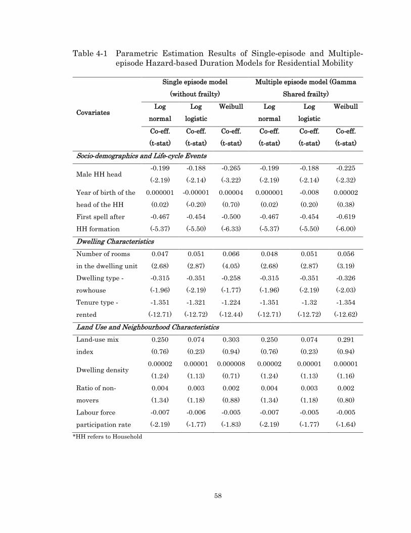
58
Table 4-1 Parametric Estimation Results of Single-episode and Multiple-
episode Hazard-based Duration Models for Residential Mobility
Covariates
Single episode model
(without frailty)
Multiple episode model (Gamma
Shared frailty)
Log
normal
Log
logistic
Weibull Log
normal
Log
logistic
Weibull
Co-eff.
(t-stat)
Co-eff.
(t-stat)
Co-eff.
(t-stat)
Co-eff.
(t-stat)
Co-eff.
(t-stat)
Co-eff.
(t-stat)
Socio-demographics and Life-cycle Events
Male HH head -0.199
(-2.19)
-0.188
(-2.14)
-0.265
(-3.22)
-0.199
(-2.19)
-0.188
(-2.14)
-0.225
(-2.32)
Year of birth of the
head of the HH
0.000001
(0.02)
-0.00001
(-0.20)
0.00004
(0.70)
0.000001
(0.02)
-0.008
(0.20)
0.00002
(0.38)
First spell after
HH formation
-0.467
(-5.37)
-0.454
(-5.50)
-0.500
(-6.33)
-0.467
(-5.37)
-0.454
(-5.50)
-0.619
(-6.00)
Dwelling Characteristics
Number of rooms
in the dwelling unit
0.047
(2.68)
0.051
(2.87)
0.066
(4.05)
0.048
(2.68)
0.051
(2.87)
0.056
(3.19)
Dwelling type -
rowhouse
-0.315
(-1.96)
-0.351
(-2.19)
-0.258
(-1.77)
-0.315
(-1.96)
-0.351
(-2.19)
-0.326
(-2.03)
Tenure type -
rented
-1.351
(-12.71)
-1.321
(-12.72)
-1.224
(-12.44)
-1.351
(-12.71)
-1.32
(-12.72)
-1.354
(-12.62)
Land Use and Neighbourhood Characteristics
Land-use mix
index
0.250
(0.76)
0.074
(0.23)
0.303
(0.94)
0.250
(0.76)
0.074
(0.23)
0.291
(0.94)
Dwelling density 0.00002
(1.24)
0.00001
(1.13)
0.000008
(0.71)
0.00002
(1.24)
0.00001
(1.13)
0.00001
(1.16)
Ratio of non-
movers
0.004
(1.34)
0.003
(1.18)
0.002
(0.88)
0.004
(1.34)
0.003
(1.18)
0.002
(0.80)
Labour force
participation rate
-0.007
(-2.19)
-0.006
(-1.77)
-0.005
(-1.83)
-0.007
(-2.19)
-0.005
(-1.77)
-0.005
(-1.64)
*HH refers to Household
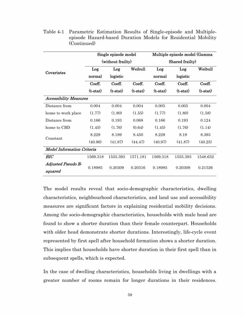
59
Table 4-1 Parametric Estimation Results of Single-episode and Multiple-
episode Hazard-based Duration Models for Residential Mobility
(Continued)
Covariates
Single episode model
(without frailty)
Multiple episode model (Gamma
Shared frailty)
Log
normal
Log
logistic
Weibull Log
normal
Log
logistic
Weibull
Coeff.
(t-stat)
Coeff.
(t-stat)
Coeff.
(t-stat)
Coeff.
(t-stat)
Coeff.
(t-stat)
Coeff.
(t-stat)
Accessibility Measures
Distance from
home to work place
0.004
(1.77)
0.004
(1.80)
0.004
(1.55)
0.005
(1.77)
0.005
(1.80)
0.004
(1.58)
Distance from
home to CBD
0.166
(1.45)
0.193
(1.76)
0.068
(0.64)
0.166
(1.45)
0.193
(1.76)
0.124
(1.14)
Constant 8.229
(40.96)
8.189
(41.87)
8.450
(44.47)
8.229
(40.97)
8.19
(41.87)
8.393
(40.25)
Model Information Criteria
BIC 1569.318 1555.393 1571.181 1569.318 1555.393 1548.632
Adjusted Pseudo R-
squared 0.18985 0.20309 0.20316 0.18985 0.20309 0.21526
The model results reveal that socio-demographic characteristics, dwelling
characteristics, neighbourhood characteristics, and land use and accessibility
measures are significant factors in explaining residential mobility decisions.
Among the socio-demographic characteristics, households with male head are
found to show a shorter duration than their female counterpart. Households
with older head demonstrate shorter durations. Interestingly, life-cycle event
represented by first spell after household formation shows a shorter duration.
This implies that households have shorter duration in their first spell than in
subsequent spells, which is expected.
In the case of dwelling characteristics, households living in dwellings with a
greater number of rooms remain for longer durations in their residences.
60
Arguably, this suggests that households with larger residences might stay for
longer duration in owned properties. Individuals living in row houses exhibit
a shorter duration. Perhaps, row houses cater to low income student groups,
who might change residential location more frequently. As anticipated, renters
are found to be more active than home owners. As renters have lower locational
capital and lesser cost of moving than owners, they are likely to move more
frequently.
Among the land use and neighbourhood characteristics, households living in
neighbourhoods with higher land-use mix index exhibit longer duration, since
neighbourhoods with greater land-use mix offer nearby services and facilities
that encourage residents to stay for a longer duration. Households living in
higher dwelling density neighbourhoods exhibit longer durations. This may be
explained by the fact that neighbourhoods with higher dwelling density have
better facilities for inhabitants, which encourage them to live there for longer
periods. Households living in stable neighbourhoods with high ratios of non-
movers stay for longer durations, as expected. Interestingly, households
exhibit shorter duration in neighbourhoods with a high labour force
participation rate.
In the case of the accessibility measures, commute distance is found to be a
significant factor for the mobility decisions. Households residing farther from
their workplace, possibly in suburban areas, demonstrate longer durations as
they generally own the property in a stable neighbourhood. Distance from
home to the CBD reveals a positive relationship. This implies that households
living nearby to the CBD are likely to relocate more frequently than
households residing in suburban areas. Thus, suburban inhabitants tend to be
more stable at a particular location after purchasing their dwellings.
In addition, a number of variables are tested during the model estimation
process. For instance, distance from home to the closest school, shopping
61
center, and transit stop, average household income in the neighbourhood, and
percentage of immigrant in the neighbourhood, among others. These variables
did not confirm priori hypotheses, as well as did not yield reasonable statistical
significance. As a result, these variables are not retained in the final model.
4.3 Residential Location Choice
Following the decision to move in the mobility stage, the next step is the
location choice. The choice of location itself has an underlying process
orientation in relation to location search and determination of location. In this
process, households first undertake a search process to identify potential
location alternatives and finally move to a location. Therefore, residential
location choice is modelled as a two-tier process of location search and location
choice. The search model assumes that households search for locations on the
basis of the residential stress. The residential stress acts as a push factor and
the characteristics of the location that holds the potential to minimize the
stress acts as a pull factor. The search model assumes that households’ search
process is constrained by their affordability. Hence, constraints regarding
household income and property value are imposed in the search model. The
proposed search model follows a fuzzy logic-based modelling method, which
offers a mechanism to recognize the release of stress by minimizing
discrepancies between the current and aspiration level. The modelling process
of fuzzy logic accommodates the stress-driven theoretical framework by
addressing the inter-dependencies between push and pull factors. The push
and pull factors continuously evolve with the changing stress of households
over their life-course.
In the final stage of location choice, households choose a location from the pool
of alternatives generated in the search process. The model follows a random
utility-based discrete choice modelling technique. To address the repeated
62
choices made by the same households during their housing career, the
conventional logit modelling methods are extended to more advanced latent
segmentation-based logit (LSL) modelling technique. The LSL model assumes
that repeated choices made by the households along their life-course are
correlated. The model captures unobserved heterogeneity by implicitly
allocating the households into discrete latent segments using a flexible
segment allocation model within the LSL framework. The inter-dependencies
between location choice and life-cycle events are explored by testing a number
of hypotheses. For example, how the plan to buy a car influences residential
location choice? does the acquisition of a car in the existing vehicle fleet and
the first time vehicle purchase have the same influence? how a change in job
affects residential location choice? and does a change in job and addition of a
job have the same influence? To explore the influence of timing of critical
events, the effect of adjustment period required to adapt prior or after an event
is tested as the lead and lagged effects. The major hypotheses regarding the
effects of adjustment period includes, how the effects of an event in anticipation
and an event on occurrence differs? and how the adjustment period varies for
different events? In addition, the study examines whether the influence of life-
cycle events varies by population segments or not? Such influence of life-
history is tested in interaction with the attributes of the location, including
parcel, accessibility, and neighbourhood characteristics. The unit of analysis
for the location model is at the parcel-level.
4.3.1 Methodology
Figure 4-2 presents a conceptual framework of the fuzzy logic-based location
search model developed in this study. The first step in the stress-based fuzzy
logic model is fuzzification that generates constraint sets for the push factors
and opportunity sets for the pull factors. The constraint sets represent input

63
sets and the opportunity sets represent output sets in the fuzzy logic modelling
framework.
Four major reasons for relocation derived from the HMTS data are considered
the push factors: to live in proximity to work/key activity locations (14.29%), to
live in desirable neighbourhood/dwelling (46.75%), due to life-cycle events
(21.56%), and other reasons (17.40%). Since households’ choices of residential
locations are strongly influenced by their affordability, such as income (Guo
and Bhat 2007) and average value of the property (Rashidi et al. 2012), this
study makes a priori assumption that each push factor is constrained by these
two parameters. Therefore, in the fuzzification stage, constraint sets in
relation to household income and average value of the property for each push
factor are generated.
The pull factors are the characteristics of locations that attract households to
consider a location to relocate. This study conceptualizes that an inter-
dependent relationship exists between the push and pull factors. For example,
households relocating to live closer to work locations are expected to search for
locations that are closer to their work place on the basis of their income and
average value of the property. Hence, the push factor “to live in proximity to
work/key activity locations” is assumed to correspond to the pull factor
“distance to work location”. In the case of households relocating to live in a
desirable neighbourhood/dwelling, households are assumed to search for
locations that have a higher percentage of non-movers in the neighbourhood.
Generally, desirable neighbourhoods refer to the neighbourhoods with reputed
schools and open spaces (i.e. park areas) in close proximity, and lower crime
rates, among others (Latkin and Curry 2003, Guo and Bhat 2002). Population
residing in such quality neighbourhoods are expected to move less frequently.
Hence, the push factor “to live in desirable neighbourhood/dwelling” is
assumed to correspond to the pull factor “percentages of non-movers in the
neighbourhood”.
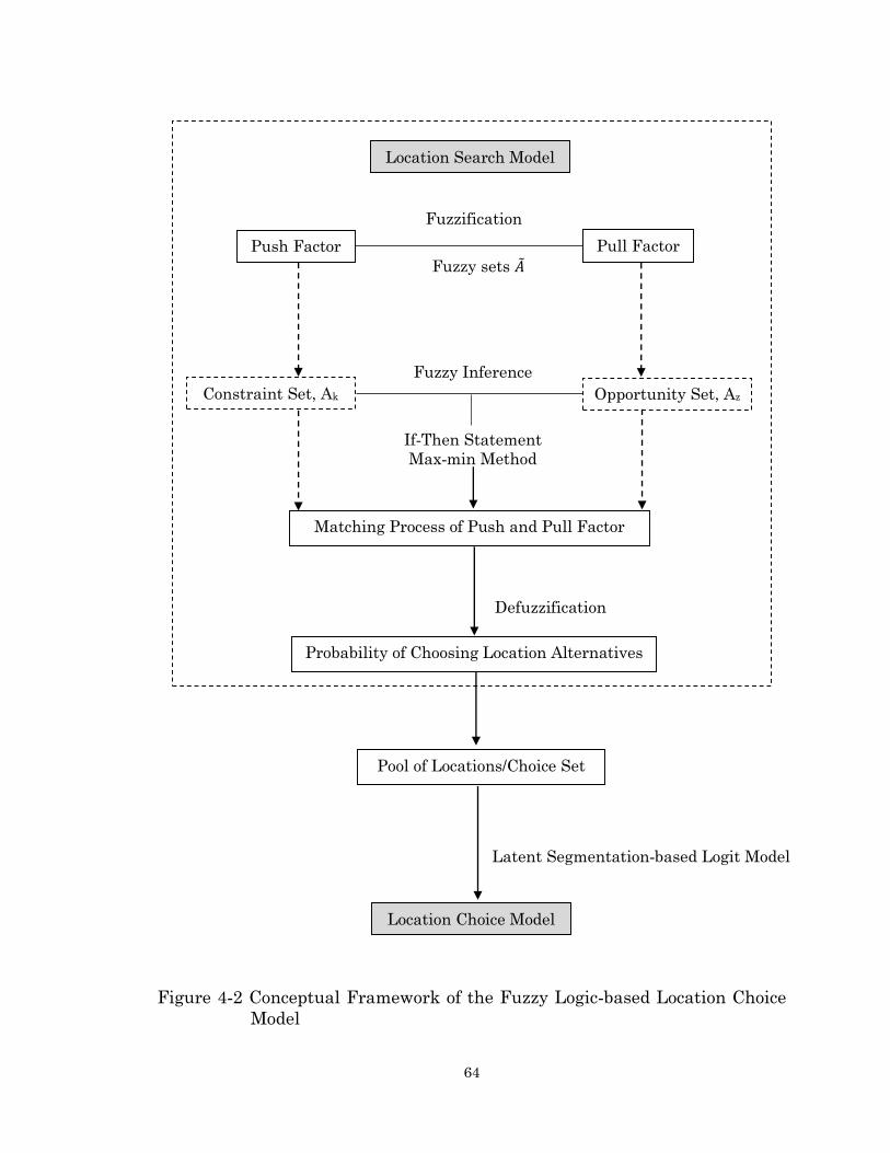
64
Figure 4-2 Conceptual Framework of the Fuzzy Logic-based Location Choice
Model
Location Search Model
Push Factor Pull Factor
Constraint Set, Ak
Opportunity Set, Az
Matching Process of Push and Pull Factor
Probability of Choosing Location Alternatives
Pool of Locations/Choice Set
Location Choice Model
Latent Segmentation-based Logit Model
Defuzzification
If-Then Statement
Max-min Method
Fuzzy sets �̃�
Fuzzification
Fuzzy Inference

65
Households relocating due to the life-cycle events are assumed to search for
locations based on the distance from CBD. Life-cycle events such as household
formation (due to marriage/living common-law) and change in household size
(due to birth of a child/death of a member/move-in or -out of members)
influence households’ decisions to live in urban or suburban/rural
neighbourhoods. For example, households with children prefer suburban
areas, since they value accessing open space, cleaner air and water (Cummins
and Jackson 2001). On the other hand, households without children prefer
urban areas, as they prioritize commuting and convenient access to different
amenities (Van Ommeren et al. 1999). In general, one of the most common
proxies used to represent urban and suburban/rural neighbourhoods is
distance to the CBD (Habib and Miller 2008). Therefore, the push factor “due
to life-cycle events” is assumed to correspond to the pull factor “distance to
CBD”. In the case of households with “other reasons”, behavioural information
regarding their reason for relocation is not available. Hence, their location
alternatives are generated using traditional method of random sampling. Since
pull factors are the attractors of a location, the fuzzy sets generated for each of
the three pull factors are termed as the opportunity sets in this study.
In the second stage, fuzzy inference, a matching process of the push and pull
factors is performed on the basis of “If-Then” statements. The most commonly
used methods to conduct fuzzy inferences are max-min and sugeno methods
(Guney and Sarikaya 2009). Sugeno method is popular in optimization
problems. In contrast, max-min is widely used for decision support modelling
due to its intuitive and interpretable nature. Moreover, max-min method offers
the flexibility of validating the scales of fuzzy membership functions using
known fuzzy rules (Teodorovic 1999, Verkuilen 2005). Therefore, this study
uses max-min method for fuzzy inferences. The third stage is defuzzification,
where household-specific probability of choosing a parcel is determined by
using the center of gravity method. The next step is to generate a pool of
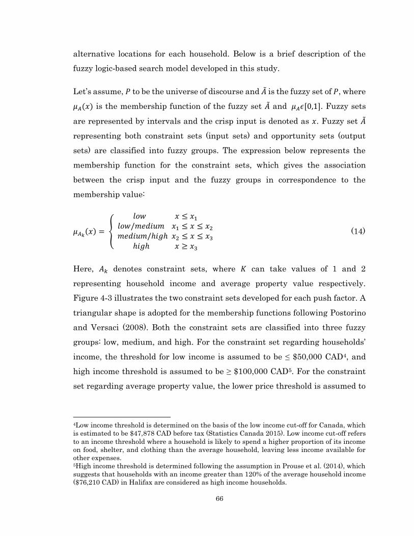
66
alternative locations for each household. Below is a brief description of the
fuzzy logic-based search model developed in this study.
Let’s assume, 𝑃 to be the universe of discourse and �̃� is the fuzzy set of 𝑃, where
𝜇𝐴(𝑥) is the membership function of the fuzzy set �̃� and 𝜇𝐴𝜖[0,1]. Fuzzy sets
are represented by intervals and the crisp input is denoted as 𝑥. Fuzzy set �̃�
representing both constraint sets (input sets) and opportunity sets (output
sets) are classified into fuzzy groups. The expression below represents the
membership function for the constraint sets, which gives the association
between the crisp input and the fuzzy groups in correspondence to the
membership value:
𝜇𝐴𝑘(𝑥) = {
𝑙𝑜𝑤 𝑥 ≤ 𝑥1
𝑙𝑜𝑤/𝑚𝑒𝑑𝑖𝑢𝑚 𝑥1 ≤ 𝑥 ≤ 𝑥2
𝑚𝑒𝑑𝑖𝑢𝑚/ℎ𝑖𝑔ℎ 𝑥2 ≤ 𝑥 ≤ 𝑥3 ℎ𝑖𝑔ℎ 𝑥 ≥ 𝑥3
(14)
Here, 𝐴𝑘 denotes constraint sets, where 𝐾 can take values of 1 and 2
representing household income and average property value respectively.
Figure 4-3 illustrates the two constraint sets developed for each push factor. A
triangular shape is adopted for the membership functions following Postorino
and Versaci (2008). Both the constraint sets are classified into three fuzzy
groups: low, medium, and high. For the constraint set regarding households’
income, the threshold for low income is assumed to be ≤ $50,000 CAD4, and
high income threshold is assumed to be ≥ $100,000 CAD5. For the constraint
set regarding average property value, the lower price threshold is assumed to
4Low income threshold is determined on the basis of the low income cut-off for Canada, which
is estimated to be $47,878 CAD before tax (Statistics Canada 2015). Low income cut-off refers
to an income threshold where a household is likely to spend a higher proportion of its income
on food, shelter, and clothing than the average household, leaving less income available for
other expenses. 5High income threshold is determined following the assumption in Prouse et al. (2014), which
suggests that households with an income greater than 120% of the average household income
($76,210 CAD) in Halifax are considered as high income households.
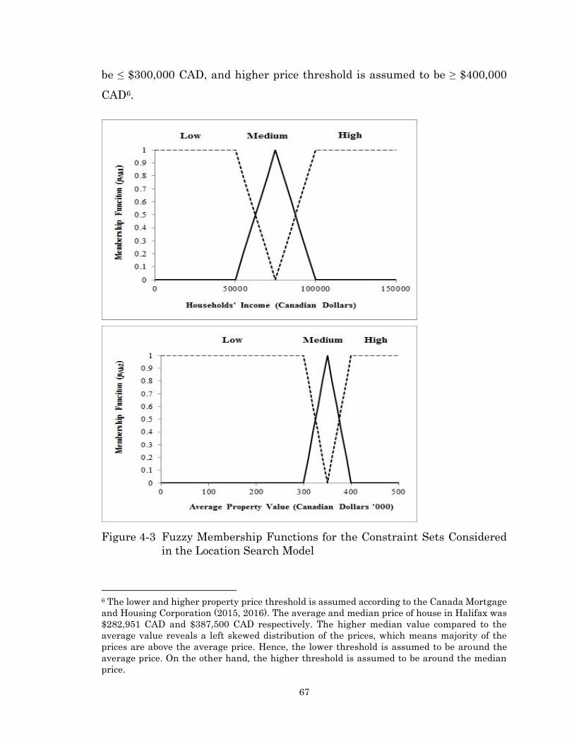
67
be ≤ $300,000 CAD, and higher price threshold is assumed to be ≥ $400,000
CAD6.
Figure 4-3 Fuzzy Membership Functions for the Constraint Sets Considered
in the Location Search Model
6 The lower and higher property price threshold is assumed according to the Canada Mortgage
and Housing Corporation (2015, 2016). The average and median price of house in Halifax was
$282,951 CAD and $387,500 CAD respectively. The higher median value compared to the
average value reveals a left skewed distribution of the prices, which means majority of the
prices are above the average price. Hence, the lower threshold is assumed to be around the
average price. On the other hand, the higher threshold is assumed to be around the median
price.

68
Assuming 𝐴𝑧 is the opportunity set and 𝜇𝐴𝑘𝑧(𝑥) is the corresponding
membership function. Here, 𝑧 can take values of 1, 2, and 3; which represent
distance to work location, percentages of non-movers in the neighbourhood,
and distance to CBD, respectively. The value of 𝑧 is conditional on the push
factor. For the push factor “to live in proximity to work/key activity locations”,
an example of the expression for the opportunity set “distance to work” can be
given as:
𝜇𝐴𝑘1(𝑥) = {
𝑔𝑜𝑜𝑑 𝑥 ≤ 0.45𝑔𝑜𝑜𝑑/𝑝𝑜𝑜𝑟 0.45 ≤ 𝑥 ≤ 0.54
𝑝𝑜𝑜𝑟 𝑥 ≥ 0.54 (15)
Similar expressions are constructed for the opportunity sets “distance to CBD”,
and “percentages of non-movers in the neighbourhood”. Figure 4-4 shows the
opportunity sets of the pull factors. Similar to the constraint sets, a triangular
shape is adopted. Each of the opportunity sets are classified into two fuzzy
groups. Opportunity set, “distance to work location” is categorized into “good”
(< 10km from the work location) and “poor” (≥ 10km from the work location)
accessibility to work place7. “Percentages of non-movers in the neighbourhood”
is classified into “not stable” (< 50% non-movers in the neighbourhood) and
“stable” (≥ 50% non-movers in the neighbourhood) neighbourhoods8. “Distance
to CBD” is categorized into “urban” (< 10km from the CBD) and “suburban and
rural” (≥ 10km from the CBD) areas9.
7 The threshold for the distance between work place and home is assumed to be 10km, since
the average commute distance in Halifax is 10.50km (Tang 2011). 8 The threshold for the percentage of non-movers in the neighbourhood is considered at the
50% point. This study assumes a neighbourhood to be stable if it has more non-movers than
movers’ population. On the other hand, if a neighbourhood has more movers than non-movers,
it is considered as a not stable neighbourhood. 9 In the context of Halifax, neighbourhoods within 10km (approximately) from the CBD that
encompasses peninsula Halifax and Dartmouth, are collectively known as “regional center” in
the Regional Planning Strategy (Halifax Regional Municipality, 2014). Hence, 10km distance
from the CBD is considered as the threshold to define urban and suburban areas.
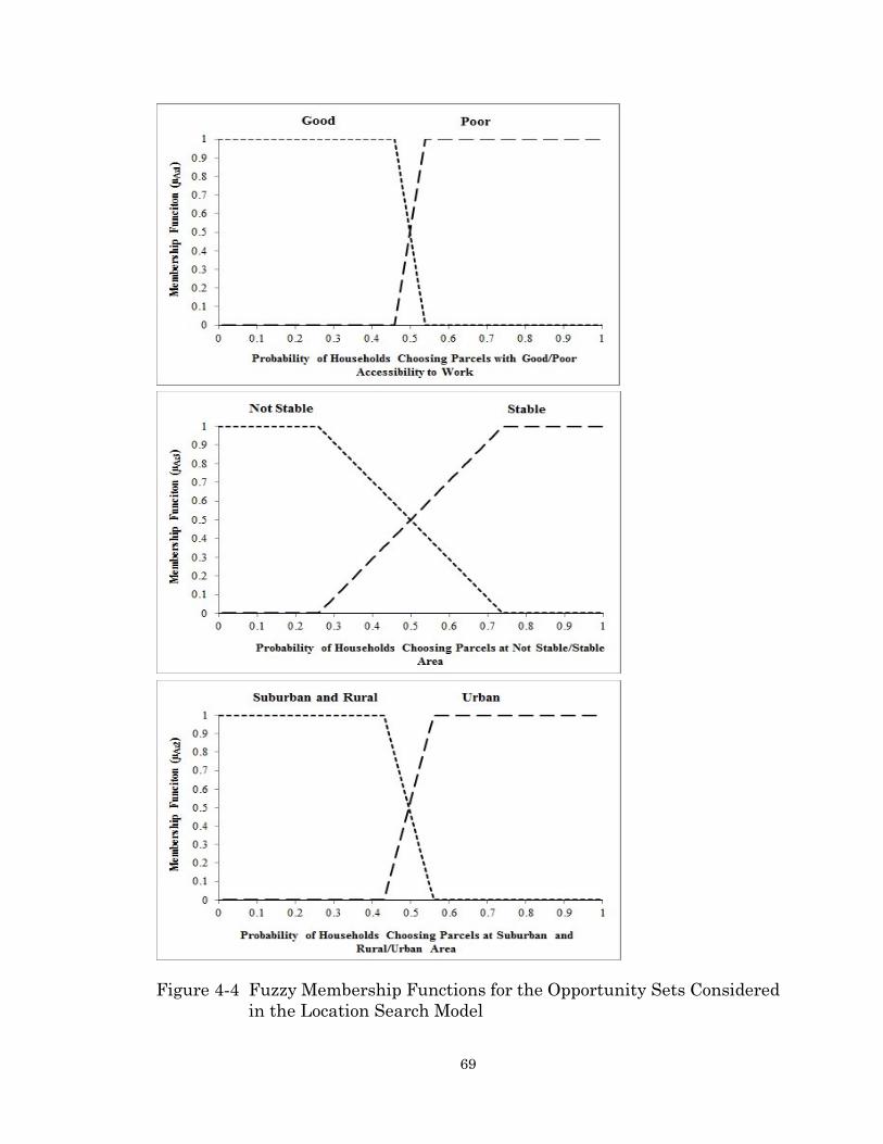
69
Figure 4-4 Fuzzy Membership Functions for the Opportunity Sets Considered
in the Location Search Model
70
Following the fuzzification stage, the matching process between a push factor
and the corresponding pull factor is conducted in the fuzzy inference stage.
Particularly, fuzzy inferences handle the degree of match between the
constraint set (If) and the opportunity set (Then) by using “If-Then” logic
statements (Andrade et al. 2006). The logic statements are derived from
observing the general trend of the data. A total of twelve logic statements are
developed for the “push-pull” combination of “to live in proximity to work/key
activity locations - distance to work location”. A typical format of the logic
statements is as follows:
IF household’s income is [HIGH] and average value of the property is [HIGH],
THEN the household chooses residential location with [GOOD] accessibility to
work place
A total of twelve and ten logic statements are developed for the “push-pull”
combinations of “to live in desirable neighbourhood/dwelling - percentages of
non-movers in the neighbourhood” and “due to life-cycle events - distance to
CBD” respectively. The logic statements developed for the “push-pull”
combinations are presented in Table 4-2.
In the fuzzy inference stage, the constraint set determines the boundaries of
the search process which results in the probability of the selection of a parcel
in the pool of alternative locations. As indicated earlier, the max-min method
is used to conduct the inferences, which can be expressed as the following
equation,
𝜇𝐴(𝑥) = 𝑚𝑎𝑥{𝑚𝑖𝑛[𝜇1(𝑥), 𝜇2(𝑥), … … 𝜇𝑛(𝑥)]} (16)
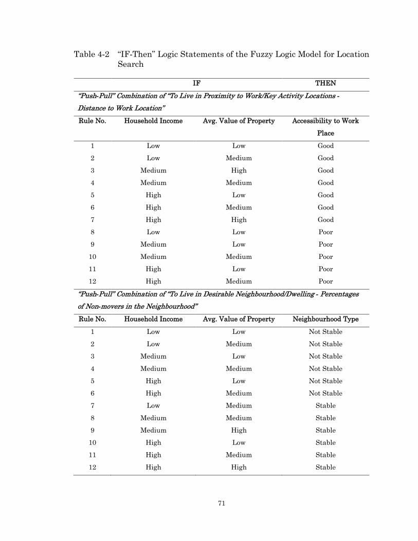
71
Table 4-2 “IF-Then” Logic Statements of the Fuzzy Logic Model for Location
Search
IF THEN
“Push-Pull” Combination of “To Live in Proximity to Work/Key Activity Locations -
Distance to Work Location”
Rule No. Household Income Avg. Value of Property Accessibility to Work
Place
1 Low Low Good
2 Low Medium Good
3 Medium High Good
4 Medium Medium Good
5 High Low Good
6 High Medium Good
7 High High Good
8 Low Low Poor
9 Medium Low Poor
10 Medium Medium Poor
11 High Low Poor
12 High Medium Poor
“Push-Pull” Combination of “To Live in Desirable Neighbourhood/Dwelling - Percentages
of Non-movers in the Neighbourhood”
Rule No. Household Income Avg. Value of Property Neighbourhood Type
1 Low Low Not Stable
2 Low Medium Not Stable
3 Medium Low Not Stable
4 Medium Medium Not Stable
5 High Low Not Stable
6 High Medium Not Stable
7 Low Medium Stable
8 Medium Medium Stable
9 Medium High Stable
10 High Low Stable
11 High Medium Stable
12 High High Stable
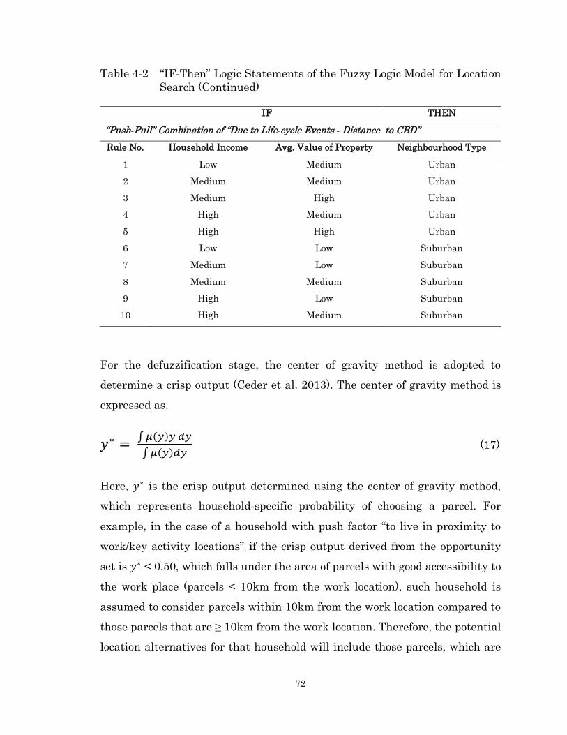
72
Table 4-2 “IF-Then” Logic Statements of the Fuzzy Logic Model for Location
Search (Continued)
IF THEN
“Push-Pull” Combination of “Due to Life-cycle Events - Distance to CBD”
Rule No. Household Income Avg. Value of Property Neighbourhood Type
1 Low Medium Urban
2 Medium Medium Urban
3 Medium High Urban
4 High Medium Urban
5 High High Urban
6 Low Low Suburban
7 Medium Low Suburban
8 Medium Medium Suburban
9 High Low Suburban
10 High Medium Suburban
For the defuzzification stage, the center of gravity method is adopted to
determine a crisp output (Ceder et al. 2013). The center of gravity method is
expressed as,
𝑦∗ = ∫ 𝜇(𝑦)𝑦 𝑑𝑦
∫ 𝜇(𝑦)𝑑𝑦 (17)
Here, 𝑦∗ is the crisp output determined using the center of gravity method,
which represents household-specific probability of choosing a parcel. For
example, in the case of a household with push factor “to live in proximity to
work/key activity locations”, if the crisp output derived from the opportunity
set is 𝑦∗ < 0.50, which falls under the area of parcels with good accessibility to
the work place (parcels < 10km from the work location), such household is
assumed to consider parcels within 10km from the work location compared to
those parcels that are ≥ 10km from the work location. Therefore, the potential
location alternatives for that household will include those parcels, which are
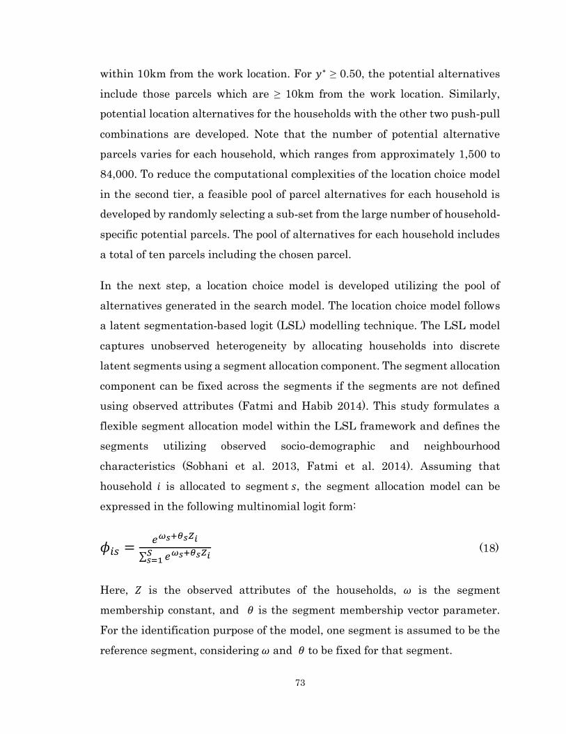
73
within 10km from the work location. For 𝑦∗ ≥ 0.50, the potential alternatives
include those parcels which are ≥ 10km from the work location. Similarly,
potential location alternatives for the households with the other two push-pull
combinations are developed. Note that the number of potential alternative
parcels varies for each household, which ranges from approximately 1,500 to
84,000. To reduce the computational complexities of the location choice model
in the second tier, a feasible pool of parcel alternatives for each household is
developed by randomly selecting a sub-set from the large number of household-
specific potential parcels. The pool of alternatives for each household includes
a total of ten parcels including the chosen parcel.
In the next step, a location choice model is developed utilizing the pool of
alternatives generated in the search model. The location choice model follows
a latent segmentation-based logit (LSL) modelling technique. The LSL model
captures unobserved heterogeneity by allocating households into discrete
latent segments using a segment allocation component. The segment allocation
component can be fixed across the segments if the segments are not defined
using observed attributes (Fatmi and Habib 2014). This study formulates a
flexible segment allocation model within the LSL framework and defines the
segments utilizing observed socio-demographic and neighbourhood
characteristics (Sobhani et al. 2013, Fatmi et al. 2014). Assuming that
household 𝑖 is allocated to segment 𝑠, the segment allocation model can be
expressed in the following multinomial logit form:
𝜙𝑖𝑠 =𝑒𝜔𝑠+𝜃𝑠𝑍𝑖
∑ 𝑒𝜔𝑠+𝜃𝑠𝑍𝑖𝑆𝑠=1
(18)
Here, 𝑍 is the observed attributes of the households, 𝜔 is the segment
membership constant, and 𝜃 is the segment membership vector parameter.
For the identification purpose of the model, one segment is assumed to be the
reference segment, considering 𝜔 and 𝜃 to be fixed for that segment.
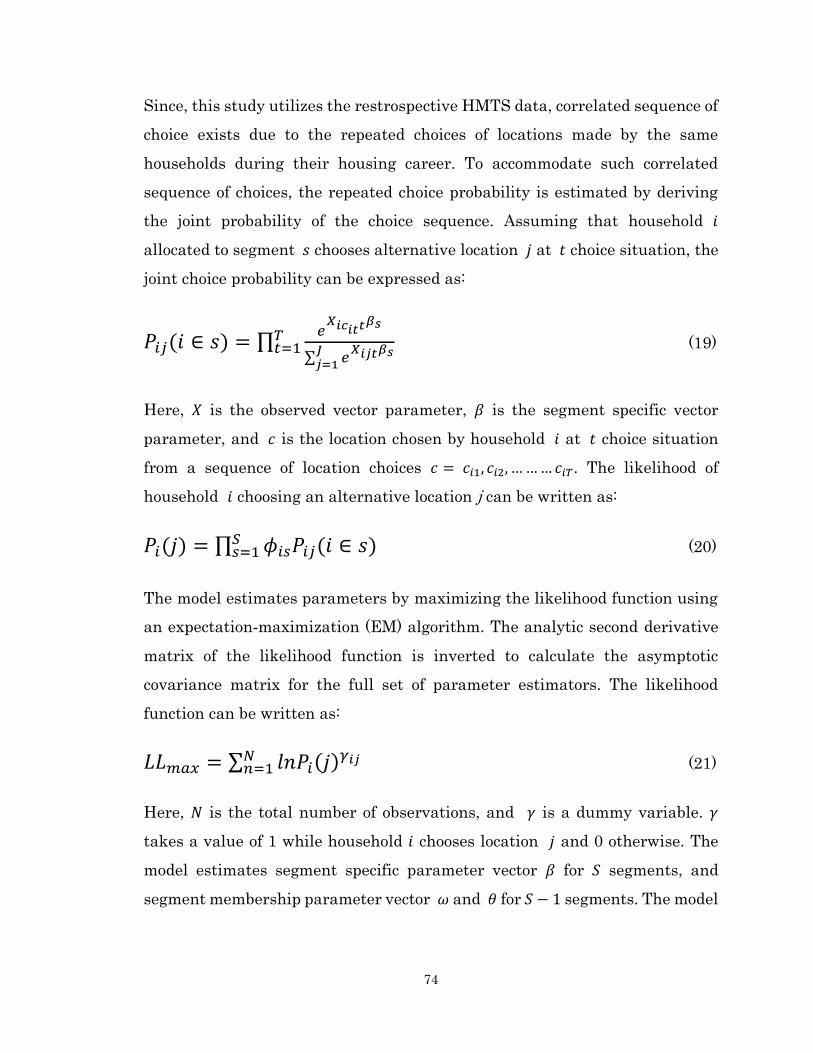
74
Since, this study utilizes the restrospective HMTS data, correlated sequence of
choice exists due to the repeated choices of locations made by the same
households during their housing career. To accommodate such correlated
sequence of choices, the repeated choice probability is estimated by deriving
the joint probability of the choice sequence. Assuming that household 𝑖
allocated to segment 𝑠 chooses alternative location 𝑗 at 𝑡 choice situation, the
joint choice probability can be expressed as:
𝑃𝑖𝑗(𝑖 ∈ 𝑠) = ∏𝑒
𝑋𝑖𝑐𝑖𝑡𝑡𝛽𝑠
∑ 𝑒𝑋𝑖𝑗𝑡𝛽𝑠𝐽
𝑗=1
𝑇𝑡=1 (19)
Here, 𝑋 is the observed vector parameter, 𝛽 is the segment specific vector
parameter, and 𝑐 is the location chosen by household 𝑖 at 𝑡 choice situation
from a sequence of location choices 𝑐 = 𝑐𝑖1, 𝑐𝑖2, … … … 𝑐𝑖𝑇. The likelihood of
household 𝑖 choosing an alternative location j can be written as:
𝑃𝑖(𝑗) = ∏ 𝜙𝑖𝑠𝑃𝑖𝑗(𝑖 ∈ 𝑠)𝑆𝑠=1 (20)
The model estimates parameters by maximizing the likelihood function using
an expectation-maximization (EM) algorithm. The analytic second derivative
matrix of the likelihood function is inverted to calculate the asymptotic
covariance matrix for the full set of parameter estimators. The likelihood
function can be written as:
𝐿𝐿𝑚𝑎𝑥 = ∑ 𝑙𝑛𝑃𝑖(𝑗)𝛾𝑖𝑗𝑁𝑛=1 (21)
Here, 𝑁 is the total number of observations, and 𝛾 is a dummy variable. 𝛾
takes a value of 1 while household 𝑖 chooses location 𝑗 and 0 otherwise. The
model estimates segment specific parameter vector 𝛽 for 𝑆 segments, and
segment membership parameter vector 𝜔 and 𝜃 for 𝑆 − 1 segments. The model
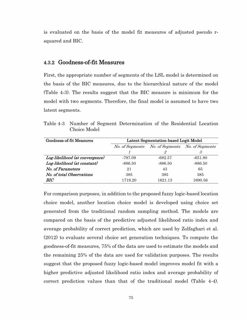
75
is evaluated on the basis of the model fit measures of adjusted pseudo r-
squared and BIC.
4.3.2 Goodness-of-fit Measures
First, the appropriate number of segments of the LSL model is determined on
the basis of the BIC measures, due to the hierarchical nature of the model
(Table 4-3). The results suggest that the BIC measure is minimum for the
model with two segments. Therefore, the final model is assumed to have two
latent segments.
Table 4-3 Number of Segment Determination of the Residential Location
Choice Model
Goodness-of-fit Measures Latent Segmentation-based Logit Model
No. of Segments
1
No. of Segments
2
No. of Segments
3
Log-likelihood (at convergence) -797.09 -682.57 -651.80
Log-likelihood (at constant) -886.50 -886.50 -886.50
No. of Parameters 21 43 65
No. of total Observations 385 385 385
BIC 1719.20 1621.13 1690.56
For comparison purposes, in addition to the proposed fuzzy logic-based location
choice model, another location choice model is developed using choice set
generated from the traditional random sampling method. The models are
compared on the basis of the predictive adjusted likelihood ratio index and
average probability of correct prediction, which are used by Zolfaghari et al.
(2012) to evaluate several choice set generation techniques. To compute the
goodness-of-fit measures, 75% of the data are used to estimate the models and
the remaining 25% of the data are used for validation purposes. The results
suggest that the proposed fuzzy logic-based model improves model fit with a
higher predictive adjusted likelihood ratio index and average probability of
correct prediction values than that of the traditional model (Table 4-4).
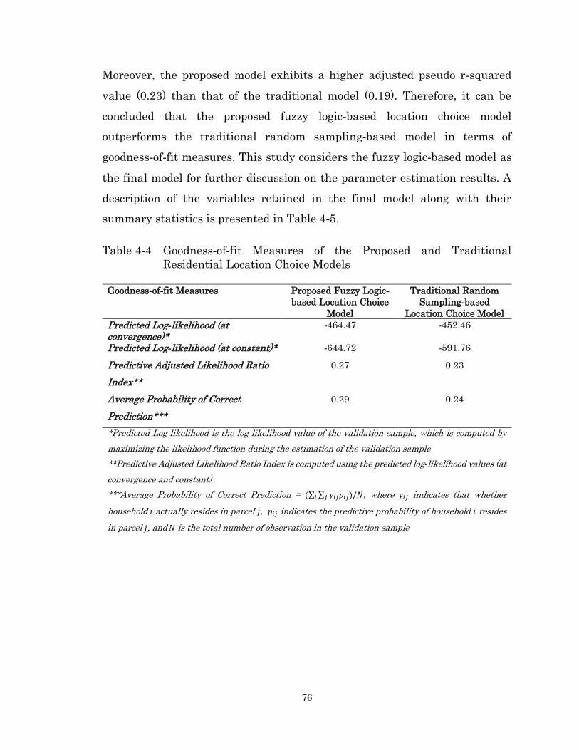
76
Moreover, the proposed model exhibits a higher adjusted pseudo r-squared
value (0.23) than that of the traditional model (0.19). Therefore, it can be
concluded that the proposed fuzzy logic-based location choice model
outperforms the traditional random sampling-based model in terms of
goodness-of-fit measures. This study considers the fuzzy logic-based model as
the final model for further discussion on the parameter estimation results. A
description of the variables retained in the final model along with their
summary statistics is presented in Table 4-5.
Table 4-4 Goodness-of-fit Measures of the Proposed and Traditional
Residential Location Choice Models
Goodness-of-fit Measures Proposed Fuzzy Logic-
based Location Choice
Model
Traditional Random
Sampling-based
Location Choice Model
Predicted Log-likelihood (at convergence)*
-464.47 -452.46
Predicted Log-likelihood (at constant)* -644.72 -591.76
Predictive Adjusted Likelihood Ratio
Index**
0.27 0.23
Average Probability of Correct
Prediction***
0.29 0.24
*Predicted Log-likelihood is the log-likelihood value of the validation sample, which is computed by
maximizing the likelihood function during the estimation of the validation sample
**Predictive Adjusted Likelihood Ratio Index is computed using the predicted log-likelihood values (at
convergence and constant)
***Average Probability of Correct Prediction = (∑ ∑ 𝑦𝑖𝑗𝑝𝑖𝑗𝑗𝑖 )/𝑁, where 𝑦𝑖𝑗 indicates that whether
household 𝑖 actually resides in parcel 𝑗, 𝑝𝑖𝑗 indicates the predictive probability of household 𝑖 resides
in parcel 𝑗, and 𝑁 is the total number of observation in the validation sample
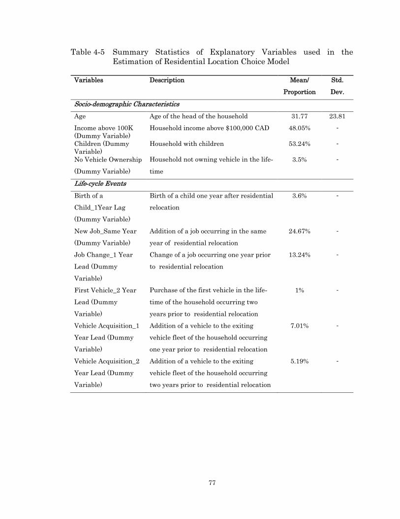
77
Table 4-5 Summary Statistics of Explanatory Variables used in the
Estimation of Residential Location Choice Model
Variables Description Mean/
Proportion
Std.
Dev.
Socio-demographic Characteristics
Age Age of the head of the household 31.77 23.81
Income above 100K
(Dummy Variable)
Household income above $100,000 CAD 48.05% -
Children (Dummy
Variable)
Household with children 53.24% -
No Vehicle Ownership
(Dummy Variable)
Household not owning vehicle in the life-
time
3.5% -
Life-cycle Events
Birth of a
Child_1Year Lag
(Dummy Variable)
Birth of a child one year after residential
relocation
3.6% -
New Job_Same Year
(Dummy Variable)
Addition of a job occurring in the same
year of residential relocation
24.67% -
Job Change_1 Year
Lead (Dummy
Variable)
Change of a job occurring one year prior
to residential relocation
13.24% -
First Vehicle_2 Year
Lead (Dummy
Variable)
Purchase of the first vehicle in the life-
time of the household occurring two
years prior to residential relocation
1% -
Vehicle Acquisition_1
Year Lead (Dummy
Variable)
Addition of a vehicle to the exiting
vehicle fleet of the household occurring
one year prior to residential relocation
7.01% -
Vehicle Acquisition_2
Year Lead (Dummy
Variable)
Addition of a vehicle to the exiting
vehicle fleet of the household occurring
two years prior to residential relocation
5.19% -
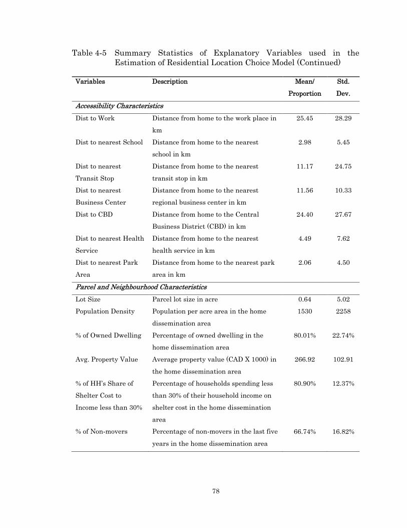
78
Table 4-5 Summary Statistics of Explanatory Variables used in the
Estimation of Residential Location Choice Model (Continued)
Variables Description Mean/
Proportion
Std.
Dev.
Accessibility Characteristics
Dist to Work Distance from home to the work place in
km
25.45 28.29
Dist to nearest School Distance from home to the nearest
school in km
2.98 5.45
Dist to nearest
Transit Stop
Distance from home to the nearest
transit stop in km
11.17 24.75
Dist to nearest
Business Center
Distance from home to the nearest
regional business center in km
11.56 10.33
Dist to CBD Distance from home to the Central
Business District (CBD) in km
24.40 27.67
Dist to nearest Health
Service
Distance from home to the nearest
health service in km
4.49 7.62
Dist to nearest Park
Area
Distance from home to the nearest park
area in km
2.06 4.50
Parcel and Neighbourhood Characteristics
Lot Size Parcel lot size in acre 0.64 5.02
Population Density Population per acre area in the home
dissemination area
1530 2258
% of Owned Dwelling Percentage of owned dwelling in the
home dissemination area
80.01% 22.74%
Avg. Property Value Average property value (CAD X 1000) in
the home dissemination area
266.92 102.91
% of HH’s Share of
Shelter Cost to
Income less than 30%
Percentage of households spending less
than 30% of their household income on
shelter cost in the home dissemination
area
80.90% 12.37%
% of Non-movers Percentage of non-movers in the last five
years in the home dissemination area
66.74% 16.82%
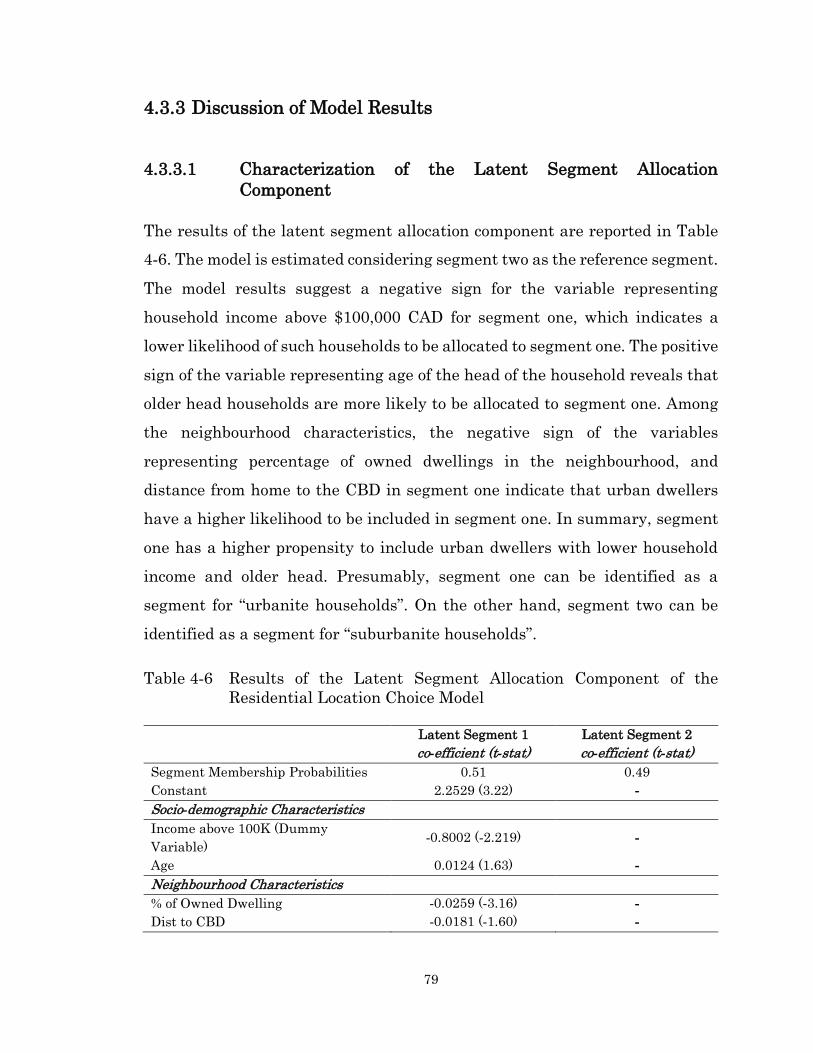
79
4.3.3 Discussion of Model Results
4.3.3.1 Characterization of the Latent Segment Allocation
Component
The results of the latent segment allocation component are reported in Table
4-6. The model is estimated considering segment two as the reference segment.
The model results suggest a negative sign for the variable representing
household income above $100,000 CAD for segment one, which indicates a
lower likelihood of such households to be allocated to segment one. The positive
sign of the variable representing age of the head of the household reveals that
older head households are more likely to be allocated to segment one. Among
the neighbourhood characteristics, the negative sign of the variables
representing percentage of owned dwellings in the neighbourhood, and
distance from home to the CBD in segment one indicate that urban dwellers
have a higher likelihood to be included in segment one. In summary, segment
one has a higher propensity to include urban dwellers with lower household
income and older head. Presumably, segment one can be identified as a
segment for “urbanite households”. On the other hand, segment two can be
identified as a segment for “suburbanite households”.
Table 4-6 Results of the Latent Segment Allocation Component of the
Residential Location Choice Model
Latent Segment 1 Latent Segment 2
co-efficient (t-stat) co-efficient (t-stat)
Segment Membership Probabilities 0.51 0.49
Constant 2.2529 (3.22) -
Socio-demographic Characteristics
Income above 100K (Dummy
Variable) -0.8002 (-2.219) -
Age 0.0124 (1.63) -
Neighbourhood Characteristics
% of Owned Dwelling -0.0259 (-3.16) -
Dist to CBD -0.0181 (-1.60) -

80
Table 4-7 Parameter Estimation Results of the Fuzzy Logic-based LSL Model
for Residential Location Choice
Variables
Latent Segmentation-based Logit Model
Latent Segment 1 Latent Segment 2
co-efficient (t-stat) co-efficient (t-stat)
Parcel Characteristics and Interaction with Life-cycle Events
Lot Size -0.1134 (-1.03) 0.1605 (2.13)
Lot Size × Birth of a Child_1Year Lag 1.2932 (1.00) 1.4578 (1.34)
Lot Size × Job Change_1 Year Lead -4.6300 (-1.00) 2.3653 (2.49)
Lot Size × New Job_Same Year 0.0979 (0.3) 0.3033 (2.10)
Accessibility Characteristics and Interaction with Life-cycle Events and Socio-demographics
Dist to Work -0.0462 (-3.23) -0.0462 (-3.23)
Dist to Work × Vehicle Acquisition_1
Year Lead 0.0049 (0.20) 0.0263 (0.44)
Dist to Work × First Vehicle_2 Year
Lead 0.0953 (1.35) 0.0953 (1.35)
Dist to Work × Children 0.0331 (1.93) -0.4197 (-8.21)
Dist to nearest School 0.4117 (2.72) -0.291 (-0.23)
Dist to nearest School × Children -0.4296 (-2.28) 0.3026 (1.86)
Dist to nearest Transit Stop -0.0081 (-0.60) -0.0081 (-0.60)
Dist to nearest Transit Stop × No Car
Ownership
-3.8791 (-1.60) -3.8791 (-1.60)
Dist to nearest Business Center 0.0230 (1.00) 0.0403 (2.08)
Dist to nearest Business Center ×
Vehicle Acquisition_2 Year Lead
0.0215 (0.23) 0.1221 (1.00)
Dist to nearest Health Service -0.0485 (-1.00) -0.4231 (-4.83)
Dist to nearest Park Area -0.3763 (-2.08) 0.2815 (1.78)
Dist to nearest Park Area × Children 0.3331 (1.40) -0.6954 (-2.20)
Neighbourhood Characteristics
Population Density 0.0001 (1.94) 0.0001 (4.77)
Avg. Property Value 0.0022 (2.18) 0.0018 (2.82)
% of HH’s Share of Shelter Cost to
Income less than 30%
0.0130 (1.32) 0.0219 (3.41)
% of Non-movers 0.1065 (10.41) -0.0266 (-4.89)
81
4.3.3.2 Discussion of the Latent Segmentation-based Logit (LSL)
Model Results
Parameter estimation results of the fuzzy logic-based LSL model are reported
in Table 4-7. A brief discussion of the model results are presented below.
4.3.3.2.1 Parcel Characteristics and Interaction with Life-cycle Events
The model results suggest that location choice is significantly influenced by
parcel characteristics. For instance, the variable representing lot size reveals
a positive relationship in segment two. Segment two is identified to include
suburbanite households who are higher income suburban dwellers.
Essentially, suburbanite households prefer larger dwellings (i.e. parcel size),
potentially in the suburban areas. In contrast, urbanite households in segment
one show a negative relationship. Interestingly, while a life-cycle event
represented by birth of a child is interacted with the lot size, a positive
relationship is found for urbanite and suburbanite households in both
segments. An increase in the household size due to the birth of a child might
trigger the requirement of a larger dwelling. Therefore, households prefer
larger-sized lots, which is consistent with the findings of Strom (2010). The
model confirms a one-year lead effect of this life-cycle event. Life-cycle event
represented by job change shows a heterogeneous behaviour as evident in
parametric values in the two segments. Households in segment two exhibit a
positive relationship. Suburbanite households in segment two belong to the
high-income group and arguably a change in job might be associated with
further increase in income. Thus, such households reveal preference for larger
dwellings following a job change. In the case of addition of a job, urbanite and
suburbanite households reveal a higher likelihood for larger-sized lots.
Addition of a job refers to increased affordability, which is expected to
positively influence the choice of larger dwellings. The model confirms a longer
adjustment period for a job change (one-year lagged effect) than that of the
82
addition of a new job (same year effect). The increased affordability associated
with the addition of a job might influence households to relocate to larger-sized
lots within a much shorter time from the occurrence of the event.
4.3.3.2.2 Accessibility Characteristics and Interaction with Life-cycle Events and Socio-demographics
In general, households are found to be more likely to reside closer to their work
place, which reflect their preferences for shorter commute distance. To
examine how vehicle transaction decisions influence location choice, the
following two variables are interacted with commute distance: vehicle
acquisition, and purchase of the first vehicle. Urbanite and suburbanite
households reveal a positive relationship for both the variables. Interestingly,
a longer adjustment period is observed for the first time vehicle purchase (two-
year lagged effect) compared to a vehicle acquisition (one-year lagged effect).
First time vehicle purchase is a key event in the life-time of the household. Due
to the limitation in time and money budgets, a longer adjustment period is
expected between two large investments of purchasing a house and first car.
When the presence of children is interacted with commute distance, a variation
in relationship is found in two segments. Suburbanite households (i.e. segment
two) who have children show a higher likelihood to reside closer to work place,
which might offer them the flexibility of trip chaining to day care centers or
schools on the way to and from work. On the other hand, urbanite households
with low income (i.e. segment one) show a higher probability to compromise
with the longer commute. Locations closer to work place might be expensive
and they might be trading off longer commute with the opportunity to reside
in proximity to other potential amenities for their children. One such amenity
might be the location of school, as argued by Kim et al. (2005). Furthermore,
when the presence of children in the household is interacted with distance to
83
the closest school, urbanite households show a higher likelihood to reside closer
to school.
Distance to the closest transit stop reveals a negative relationship.
Interestingly, when this variable is interacted with a dummy variable
representing households not owning a vehicle in their life-time, the negative
effect substantially increases. This reflects the fact that households prefer to
live closer to transit stop; however, the propensity to reside closer to transit
stop increases for households without vehicle ownership. Distance to the
nearest regional business center shows a positive relationship. Since,
households prefer locations farther away from regional business centers, which
is characterized as big-box retails in the case of Halifax. A similar positive
relationship is found while distance to the nearest regional business center is
interacted with vehicle acquisition. This result reflects that addition of a
vehicle might offer added freedom and convenience for longer trips.
Households exhibit a higher probability to choose locations closer to the health
care services, since locations closer to health services offer easier access to daily
and periodic medical services. Distance to the closest park area exhibits
heterogeneous relationship in the two segments. Urbanite households are
found to be extremely sensitive to distance to the nearest park area and prefer
to live closer to park area. Locations closer to park areas are preferable due to
the convenient access to open space, which can serve as a regular recreational
place for the household members. In contrast, households in segment two
reveal a positive relationship. Interestingly, while distance to the closest park
area is interacted with presence of children in the household, suburbanite
households exhibit a strong preference for locations closer to park areas. In
summary, the model results reflect that the effects of accessibility
characteristics in choosing home locations are substantially dictated by life-
cycle events.

84
4.3.3.2.3 Neighbourhood Characteristics
Regarding the neighbourhood characteristics, households have a higher
probability to live in neighbourhoods with higher population density. Average
property value in the neighbourhood shows a positive relationship, since
higher average property value indicates high income neighbourhoods with
better housing and access to diversified amenities (Guo and Bhat 2002), which
are expected to be desirable. The variable representing percentage of
households with a shelter cost to income share of less than 30% reflects high
income neighbourhoods with more disposable income after housing related
payments. This variable exhibits a strong positive relationship, which extends
the fact that locations with more disposable income are more attractive.
Interestingly, stable neighbourhoods represented by percentage of non-movers
show significant variations between the two segments. Urbanite households
prefer stable neighbourhoods and suburbanite households show affinity to
evolving neighbourhoods in Halifax. This result is a deviation from an earlier
Toronto study (Habib and Miller 2009), in which households generally
preferred stable neighbourhoods. This may reflect a unique continual growth
of new subdivisions in Halifax, which has become an interesting feature of the
city as documented in Brewer and Grant (2015).
In addition to the above discussed variables, the model tests a number of
variables such as, death of a member, member move out, loss of a job, distance
to the nearest shopping center, average household income, employment rate,
percentage of immigrant, and land-use mix index. These variables could not be
included in the final model due to discrepancies in the hypothesis confirmation
along with reasonable statistical significance. The model also could not confirm
statistically significant effects of how neighbourhood characteristics varies by
life-cycle events. One of the possible attributing factors might be the
unavailability of historical records for changes in urban form.
85
4.4 Modelling Mode Transitions
This research offers insights towards how a change in one life-domain is
associated with a change in another domain. Particularly, this study
investigates how residential relocation decisions influence individuals to
change their commute mode. The study conceptualizes that individuals
reassess their commute mode when they relocate to a new location. Following
reappraisal, they either continue using the same mode, which is considered
mode loyalty, or make a transition to a new mode, which is considered mode
transition. In this study, the mode transition scenario is developed by
comparing the choice of commute mode between two distinct temporal points
of consecutive residential locations, which offers the opportunity to examine
how changes in socio-demographic and accessibility characteristics between
these two temporal points affect the decision. These transitional variables are
generated by comparing household characteristics between two subsequent
residential locations. In addition, the effects of life-cycle events are tested. To
account for the correlated sequence of repeated choices of the same individuals
over their life-time, a random-parameters logit (RPL) model is developed. The
model also captures unobserved heterogeneity.
4.4.1 Modelling Methods
This study utilizes the retrospective HMTS data to generate the mode
transition scenarios. A sample of 288 households are utilized from the HMTS
data, who have reported at least two consecutive housing records. The dataset
yields a total sample of 453 mode loyalty and transition instances. The mode
loyalty and transitions are determined by comparing the choice of commute
This section is largely derived from the following journal paper:
Fatmi, M.R., and Habib, M.A. (2016). Life-Oriented Approach of Modelling of Commute
Mode Loyalty and Transition Behaviour. Transportation Research Record: Journal of Transportation Research Board, 2565(1), 37-47.
86
mode in two consecutive residential locations. The results reveal that 67.10%
respondents are loyal to the commute mode used at their previous location and
continue with the same one at the subsequent location. On the other hand,
32.90% of the respondents make a transition in commute mode when moving
to a new location. To understand mode-specific transition and loyalty, this
study considers the following nine choice scenarios as the dependent variable:
1. Loyal to Car: respondent’s primary commute mode is car in their prior and
subsequent location
2. Loyal to Transit: respondent’s primary commute mode is transit in their
prior and subsequent location
3. Loyal to Active Transportation: respondent’s primary commute mode is
active transportation (walk/bike) in their prior and subsequent location
4. Transition from Car to Transit: respondent makes a transition in primary
commute mode from car in prior location to transit in subsequent location
5. Transition from Car to Active Transportation: respondent makes a
transition in primary commute mode from car in prior location to active
transportation in subsequent location
6. Transition from Transit to Car: respondent makes a transition in primary
commute mode from transit in prior location to car in subsequent location
7. Transition from Transit to Active Transportation: respondent makes a
transition in primary commute mode from transit in prior location to active
transportation in subsequent location
8. Transition from Active Transportation to Car: respondent makes a
transition in primary commute mode from active transportation in prior
location to car in subsequent location
9. Transition from Active Transportation to Transit: respondent makes a
transition in primary commute mode from active transportation in prior
location to transit in subsequent location
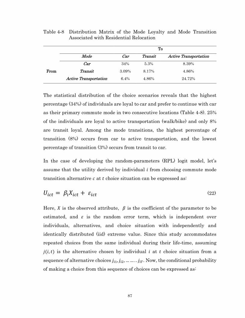
87
Table 4-8 Distribution Matrix of the Mode Loyalty and Mode Transition
Associated with Residential Relocation
To
Mode Car Transit Active Transportation
From
Car 34% 5.3% 8.39%
Transit 3.09% 8.17% 4.86%
Active Transportation 6.4% 4.86% 24.72%
The statistical distribution of the choice scenarios reveals that the highest
percentage (34%) of individuals are loyal to car and prefer to continue with car
as their primary commute mode in two consecutive locations (Table 4-8). 25%
of the individuals are loyal to active transportation (walk/bike) and only 8%
are transit loyal. Among the mode transitions, the highest percentage of
transition (8%) occurs from car to active transportation, and the lowest
percentage of transition (3%) occurs from transit to car.
In the case of developing the random-parameters (RPL) logit model, let’s
assume that the utility derived by individual 𝑖 from choosing commute mode
transition alternative 𝑐 at 𝑡 choice situation can be expressed as:
𝑈𝑖𝑐𝑡 = 𝛽i𝑋𝑖𝑐𝑡 + 휀𝑖𝑐𝑡 (22)
Here, 𝑋 is the observed attribute, 𝛽 is the coefficient of the parameter to be
estimated, and 휀 is the random error term, which is independent over
individuals, alternatives, and choice situation with independently and
identically distributed (iid) extreme value. Since this study accommodates
repeated choices from the same individual during their life-time, assuming
𝑗(𝑖, 𝑡) is the alternative chosen by individual 𝑖 at 𝑡 choice situation from a
sequence of alternative choices 𝑗𝑖1, 𝑗𝑖2, … … . . 𝑗𝑖𝑇. Now, the conditional probability
of making a choice from this sequence of choices can be expressed as:
88
𝑃𝑖(𝛽i) = ∏𝑒
𝛽i 𝑋𝑖𝑗(𝑖,𝑡)𝑡
∑ 𝑒𝛽i𝑋𝑖𝑐𝑡𝑚
𝑇𝑡=1 (23)
Here, 𝑚 is the total number of alternatives. This choice probability is
conditional on 𝛽. Interestingly, the analyst observes 𝑋 and does not observe 𝛽.
Therefore, the choice probability cannot be conditional on 𝛽, and the
unconditional choice probability is derived by integrating conditional
probability over all possible values of 𝛽. The unconditional choice probability
can be written as following:
𝑃𝑖 = ∫ ∏𝑒
𝛽i 𝑋𝑖𝑗(𝑖,𝑡)𝑡
∑ 𝑒𝛽i𝑋𝑖𝑐𝑡𝑚
𝑇𝑡=1 𝑓(𝛽i|𝜇, 𝜗)𝑑𝛽i (24)
Here, 𝛽 is distributed over each individual with a density function of 𝑓(𝛽i|𝜇, 𝜗),
where, 𝜇 and 𝜗 are the mean and standard deviation of the function. This study
assumes a normal distribution of the density function, following a similar
assumption by Revelt and Train (1998). 𝛽 is an individual specific parameter,
representing individual’s taste and other associated unobserved factors.
Individual’s taste and unobserved factors might vary among the sample
population, which could be captured by estimating the parameters (𝜇, 𝜗) of the
density function. One approach for estimating the choice probability is by
maximizing the likelihood function: 𝐿𝐿 = ∑ 𝑙𝑛 𝑃𝑖𝐼𝑖=1 . This likelihood function
cannot be maximized analytically, since it is a multivariate integral. Therefore,
the probabilities are estimated through simulation. In this process, a value of
𝛽 is drawn from the density function 𝑓(𝛽i|𝜇, 𝜗) and considered as the first draw.
Using this draw, the corresponding choice probability is estimated. Similarly,
several draws of 𝛽 are taken and corresponding choice probabilities are
estimated. Finally, the average of the choice probabilities from several draws
is estimated in order to approximate the choice probability, which can be
expressed as:
89
𝑃�̅� =1
𝑅 ∑ 𝑃𝑖(βi
r)𝑅𝑟=1 (25)
Here, 𝑃�̅� is the average of the simulated choice probability, which is an unbiased
estimator of the unconditional choice probability 𝑃𝑖, 𝑅 is the total number of
draws, and βir is the rth draw from 𝑓(𝛽i|𝜇, 𝜗). The variance of 𝑃�̅� decreases as 𝑅
increases. 𝑃�̅� is smooth (twice differentiable) and facilitates the numerical
search for the maximum likelihood function. The simulated log likelihood
function is developed using the average of the simulated probabilities and can
be expressed as:
𝑆𝐿 = ∑ ln 𝑃�̅�𝐼𝑖=1 = ∑ ln
1
𝑅 ∑ 𝑃𝑖(βi
r)𝑅𝑟=1
𝐼𝑖=1 (26)
Here, 𝐼 is the total number of observations. This simulated log likelihood is
maximized for 500 Halton draws using a Monte-Carlo simulation approach.
Monte-Carlo simulation approach generates a faster convergence rate
compared to other methods (Train 2003.). Moreover, the use of Halton draws
improves the performance of Monte-Carlo simulation compared to random
draws (Bhat 2003). The model estimates coefficient parameter 𝛽, and 𝜇 and 𝜗
of the density function. For comparison purposes, a conventional multinomial
logit model (MNL) is developed. The models are compared on the basis of
goodness-of-fit measures of adjusted pseudo r-squared, and likelihood ratio
test.
4.4.2 Model Results
This study examines the effects of life-cycle events. One of the key features of
the study is to test the effects of life-oriented socio-demographic and
accessibility related transitional variables. The dynamic nature of the mode
transition phenomenon offers the opportunity to derive life-oriented socio-
demographic transitional variables by comparing socio-demographic

90
information between two subsequent residential locations. Such transitional
variables refer to the change in individuals’ socio-demographic and dwelling
characteristics in the current residential location compared to the previous
location. Socio-demographic transitional variables include increase and
decrease in household income, car ownership, and number of bedroom, as well
as transition from rented to owned dwelling and vice versa. Similarly,
transitional variables for accessibility measures to different activity points and
transportation services are estimated; which include moving closer to or
farther away from work location, transit station, or central business district
(CBD), as well as other accessibility-related transitional variables. In addition,
socio-demographic, accessibility, land use, and neighbourhood characteristics
are considered during the model estimation process. Table 4-9 presents the
summary statistics of the variables retained in the final model.
For comparison purposes, a multinomial logit (MNL) model is developed in
addition to the RPL model. The goodness-of-fit measures suggest that the RPL
model performs better with a higher adjusted pseudo r-squared value
compared to the MNL model. In addition, the RPL model outperforms the MNL
model with a chi-squared statistic of 388.49 (critical value of chi-square 106.32
with 75 degrees of freedom) at the 1% significance level. Therefore, the RPL
model is considered as the final model. The model estimation results of the
RPL model is presented in Table 4-10.
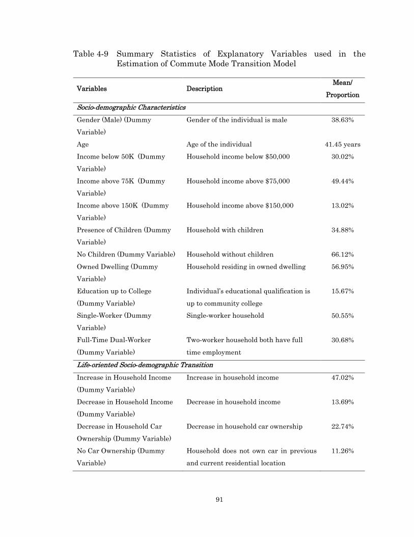
91
Table 4-9 Summary Statistics of Explanatory Variables used in the
Estimation of Commute Mode Transition Model
Variables Description Mean/
Proportion
Socio-demographic Characteristics
Gender (Male) (Dummy
Variable)
Gender of the individual is male 38.63%
Age Age of the individual 41.45 years
Income below 50K (Dummy
Variable)
Household income below $50,000 30.02%
Income above 75K (Dummy
Variable)
Household income above $75,000 49.44%
Income above 150K (Dummy
Variable)
Household income above $150,000 13.02%
Presence of Children (Dummy
Variable)
Household with children 34.88%
No Children (Dummy Variable) Household without children 66.12%
Owned Dwelling (Dummy
Variable)
Household residing in owned dwelling 56.95%
Education up to College
(Dummy Variable)
Individual’s educational qualification is
up to community college
15.67%
Single-Worker (Dummy
Variable)
Single-worker household 50.55%
Full-Time Dual-Worker
(Dummy Variable)
Two-worker household both have full
time employment
30.68%
Life-oriented Socio-demographic Transition
Increase in Household Income
(Dummy Variable)
Increase in household income 47.02%
Decrease in Household Income
(Dummy Variable)
Decrease in household income 13.69%
Decrease in Household Car
Ownership (Dummy Variable)
Decrease in household car ownership 22.74%
No Car Ownership (Dummy
Variable)
Household does not own car in previous
and current residential location
11.26%

92
Table 4-9 Summary Statistics of Explanatory Variables used in the
Estimation of Commute Mode Transition Model (Continued)
Variables Description Mean/
Proportion
Life-oriented Socio-demographic Transition (Continued)
Increase in Number of
Bedrooms (Dummy Variable)
Increase in number of bedrooms 39.96%
Decrease in Number of Rooms
(Dummy Variable)
Decrease in number of rooms 30.02%
Moved from Rented to Owned
(Dummy Variable)
Individual relocating from rented to
owned dwelling
26.27%
Moved from Owned to Rented
(Dummy Variable)
Individual relocating from owned to
rented dwelling
10.15%
Life-cycle Events
Birth of a Child_1 Year Lead
(Dummy Variable)
Birth of a child 1 year prior to commute
mode transition
11.04%
New Household Formation
(Dummy Variable)
Reason for residential relocation is the
formation of new household
10.38%
Addition of a Job_1 Year Lead
(Dummy Variable)
Addition of a job 1 year prior to commute
mode transition
16.56%
Addition of a Job_2 Year Lead
(Dummy Variable)
Addition of a job 2 year prior to commute
mode transition
12.58%
Lost Job_1 Year Lead (Dummy
Variable)
Lost job 1 year prior to commute mode
transition
9.71%
Lost Job_2 Year Lead (Dummy
Variable)
Lost job 2 year prior to commute mode
transition
6.62%
Addition of Car_Same Year
(Dummy Variable)
Addition of a car to the household vehicle
fleet in the same year of commute mode
transition
19.42%
Traded Car_Same Year
(Dummy Variable)
Household traded car in the same year of
commute mode transition
18.98%
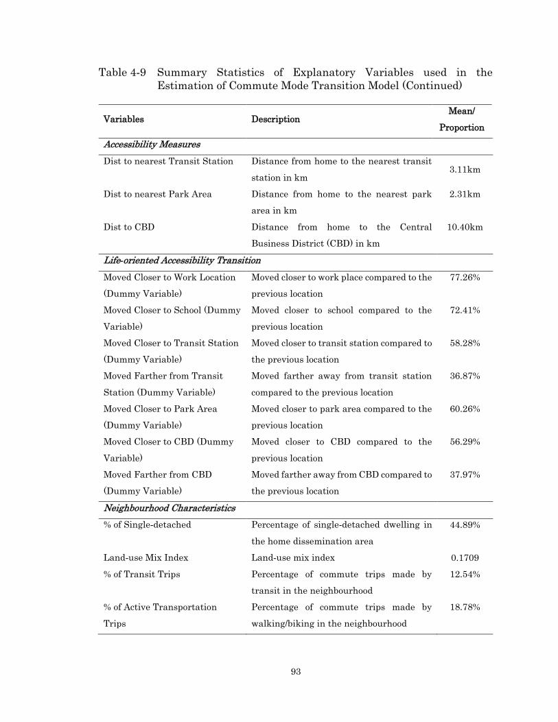
93
Table 4-9 Summary Statistics of Explanatory Variables used in the
Estimation of Commute Mode Transition Model (Continued)
Variables Description Mean/
Proportion
Accessibility Measures
Dist to nearest Transit Station Distance from home to the nearest transit
station in km 3.11km
Dist to nearest Park Area Distance from home to the nearest park
area in km
2.31km
Dist to CBD Distance from home to the Central
Business District (CBD) in km
10.40km
Life-oriented Accessibility Transition
Moved Closer to Work Location
(Dummy Variable)
Moved closer to work place compared to the
previous location
77.26%
Moved Closer to School (Dummy
Variable)
Moved closer to school compared to the
previous location
72.41%
Moved Closer to Transit Station
(Dummy Variable)
Moved closer to transit station compared to
the previous location
58.28%
Moved Farther from Transit
Station (Dummy Variable)
Moved farther away from transit station
compared to the previous location
36.87%
Moved Closer to Park Area
(Dummy Variable)
Moved closer to park area compared to the
previous location
60.26%
Moved Closer to CBD (Dummy
Variable)
Moved closer to CBD compared to the
previous location
56.29%
Moved Farther from CBD
(Dummy Variable)
Moved farther away from CBD compared to
the previous location
37.97%
Neighbourhood Characteristics
% of Single-detached Percentage of single-detached dwelling in
the home dissemination area
44.89%
Land-use Mix Index Land-use mix index 0.1709
% of Transit Trips Percentage of commute trips made by
transit in the neighbourhood
12.54%
% of Active Transportation
Trips
Percentage of commute trips made by
walking/biking in the neighbourhood
18.78%
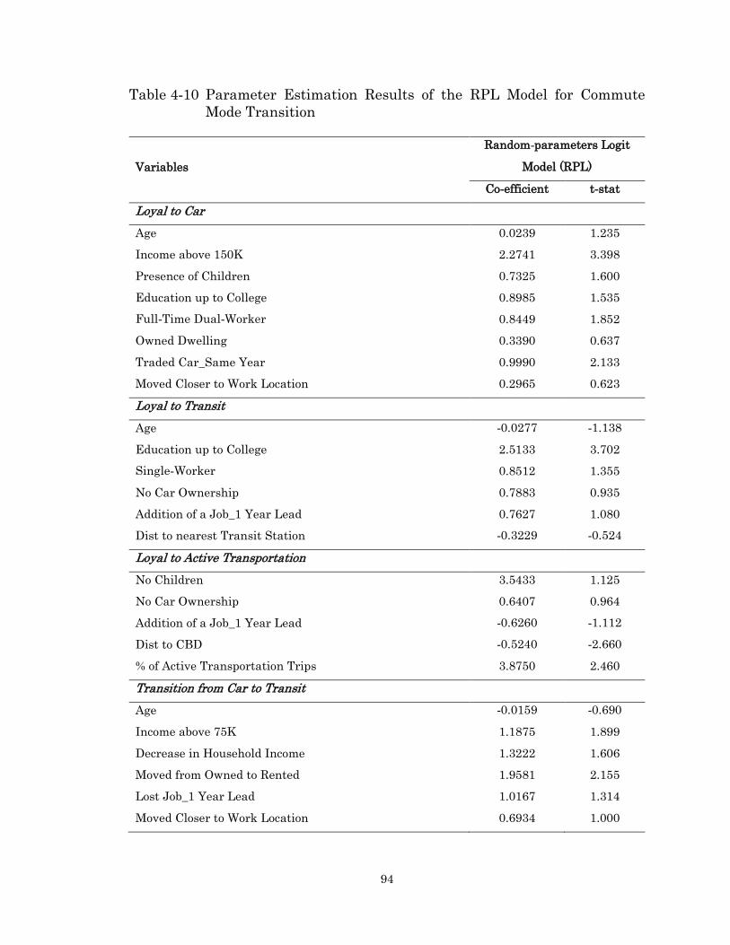
94
Table 4-10 Parameter Estimation Results of the RPL Model for Commute
Mode Transition
Variables
Random-parameters Logit
Model (RPL)
Co-efficient t-stat
Loyal to Car
Age 0.0239 1.235
Income above 150K 2.2741 3.398
Presence of Children 0.7325 1.600
Education up to College 0.8985 1.535
Full-Time Dual-Worker 0.8449 1.852
Owned Dwelling 0.3390 0.637
Traded Car_Same Year 0.9990 2.133
Moved Closer to Work Location 0.2965 0.623
Loyal to Transit
Age -0.0277 -1.138
Education up to College 2.5133 3.702
Single-Worker 0.8512 1.355
No Car Ownership 0.7883 0.935
Addition of a Job_1 Year Lead 0.7627 1.080
Dist to nearest Transit Station -0.3229 -0.524
Loyal to Active Transportation
No Children 3.5433 1.125
No Car Ownership 0.6407 0.964
Addition of a Job_1 Year Lead -0.6260 -1.112
Dist to CBD -0.5240 -2.660
% of Active Transportation Trips 3.8750 2.460
Transition from Car to Transit
Age -0.0159 -0.690
Income above 75K 1.1875 1.899
Decrease in Household Income 1.3222 1.606
Moved from Owned to Rented 1.9581 2.155
Lost Job_1 Year Lead 1.0167 1.314
Moved Closer to Work Location 0.6934 1.000
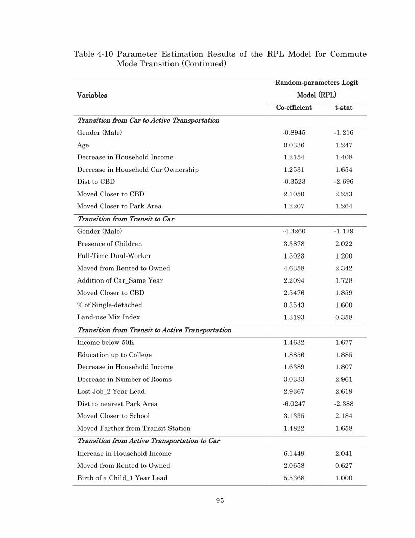
95
Table 4-10 Parameter Estimation Results of the RPL Model for Commute
Mode Transition (Continued)
Variables
Random-parameters Logit
Model (RPL)
Co-efficient t-stat
Transition from Car to Active Transportation
Gender (Male) -0.8945 -1.216
Age 0.0336 1.247
Decrease in Household Income 1.2154 1.408
Decrease in Household Car Ownership 1.2531 1.654
Dist to CBD -0.3523 -2.696
Moved Closer to CBD 2.1050 2.253
Moved Closer to Park Area 1.2207 1.264
Transition from Transit to Car
Gender (Male) -4.3260 -1.179
Presence of Children 3.3878 2.022
Full-Time Dual-Worker 1.5023 1.200
Moved from Rented to Owned 4.6358 2.342
Addition of Car_Same Year 2.2094 1.728
Moved Closer to CBD 2.5476 1.859
% of Single-detached 0.3543 1.600
Land-use Mix Index 1.3193 0.358
Transition from Transit to Active Transportation
Income below 50K 1.4632 1.677
Education up to College 1.8856 1.885
Decrease in Household Income 1.6389 1.807
Decrease in Number of Rooms 3.0333 2.961
Lost Job_2 Year Lead 2.9367 2.619
Dist to nearest Park Area -6.0247 -2.388
Moved Closer to School 3.1335 2.184
Moved Farther from Transit Station 1.4822 1.658
Transition from Active Transportation to Car
Increase in Household Income 6.1449 2.041
Moved from Rented to Owned 2.0658 0.627
Birth of a Child_1 Year Lead 5.5368 1.000
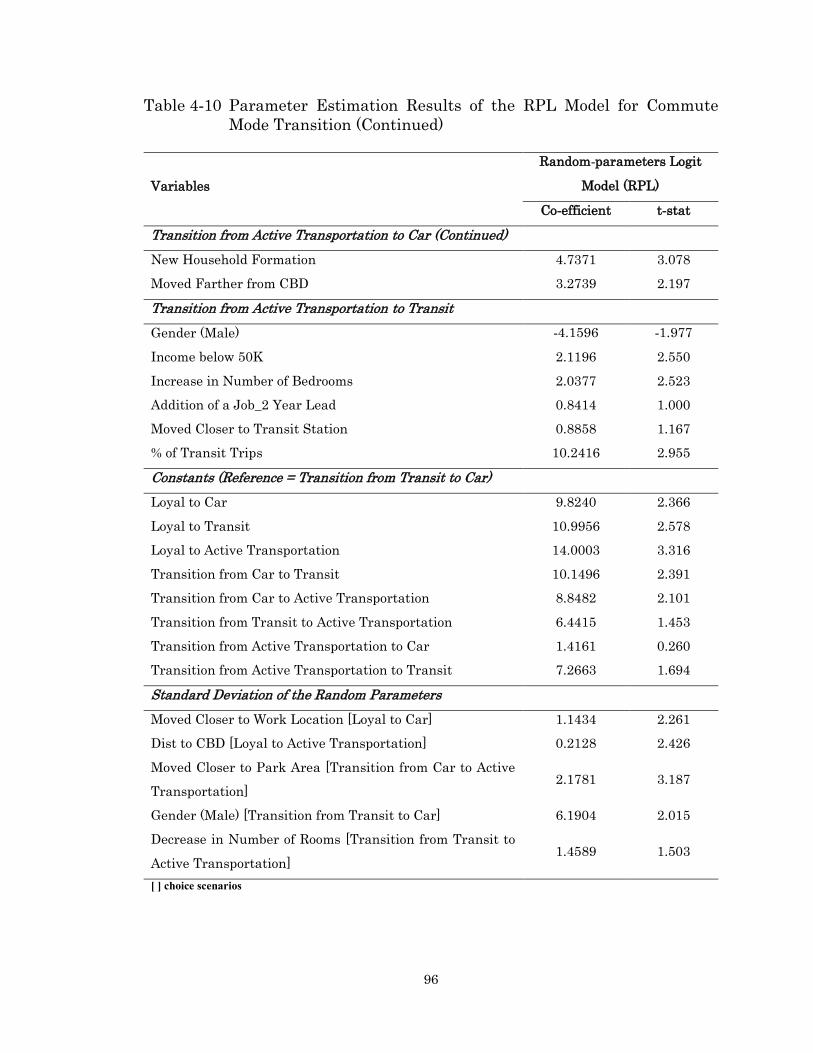
96
Table 4-10 Parameter Estimation Results of the RPL Model for Commute
Mode Transition (Continued)
Variables
Random-parameters Logit
Model (RPL)
Co-efficient t-stat
Transition from Active Transportation to Car (Continued)
New Household Formation 4.7371 3.078
Moved Farther from CBD 3.2739 2.197
Transition from Active Transportation to Transit
Gender (Male) -4.1596 -1.977
Income below 50K 2.1196 2.550
Increase in Number of Bedrooms 2.0377 2.523
Addition of a Job_2 Year Lead 0.8414 1.000
Moved Closer to Transit Station 0.8858 1.167
% of Transit Trips 10.2416 2.955
Constants (Reference = Transition from Transit to Car)
Loyal to Car 9.8240 2.366
Loyal to Transit 10.9956 2.578
Loyal to Active Transportation 14.0003 3.316
Transition from Car to Transit 10.1496 2.391
Transition from Car to Active Transportation 8.8482 2.101
Transition from Transit to Active Transportation 6.4415 1.453
Transition from Active Transportation to Car 1.4161 0.260
Transition from Active Transportation to Transit 7.2663 1.694
Standard Deviation of the Random Parameters
Moved Closer to Work Location [Loyal to Car] 1.1434 2.261
Dist to CBD [Loyal to Active Transportation] 0.2128 2.426
Moved Closer to Park Area [Transition from Car to Active
Transportation] 2.1781 3.187
Gender (Male) [Transition from Transit to Car] 6.1904 2.015
Decrease in Number of Rooms [Transition from Transit to
Active Transportation] 1.4589 1.503
[ ] choice scenarios

97
Table 4-10 Parameter Estimation Results of the RPL Model for Commute
Mode Transition (Continued)
Variables
Random-parameters Logit
Model (RPL)
Co-efficient t-stat
Standard Deviation of the Random Parameters (Continued)
Moved Farther from Transit Station [Transition from
Transit to Active Transportation] 1.3034 1.635
Moved from Rented to Owned [Transition from Active
Transportation to Car] 5.8190 2.160
Gender (Male) [Transition from Active Transportation to
Transit] 3.2471 2.450
Goodness-of-fit Measures
Log-likelihood (at Convergence) -354.4494
Log-likelihood (at Constant) -548.6948
Adjusted Pseudo R-squared 0.3540
[ ] choice scenarios
4.4.2.1 Discussion of the Random-parameters Logit (RPL) Model
Results
4.4.2.1.1 Loyal to Car
Model results suggest that older individuals are more likely to be car loyal, as
probability of remaining loyal to car increases with age. Similarly, the high
income group, characterized by household income above $150000, two-worker
household both having full time job status, and individual residing in an owned
dwelling, prefers to be car loyal for commuting. Presence of children in the
household is positively associated with car loyalty, since individuals might
require a car to travel with children, for example, trip chain to day care
centers/schools on their way to work. Trading (i.e., changing) car and
residential relocation occurring in the same year is associated with a higher
likelihood of continuing to commute by car. This result might relate to high
98
income individuals’ self-selecting car as their commute mode following
residential relocation, or it may represent a reverse causality. Surprisingly,
relocating to a location closer to the workplace than the previous location
reveals a higher probability to continue commuting with car. However, this
variable yields a statistically significant standard deviation, with a mean and
standard deviation of 0.2965 and 1.1434, respectively. This large standard
deviation suggests that a sizable variation exists among the individuals in
being car loyal if their commute distance is shortened. Therefore, shortening
commute distance does not necessarily trigger a change in mode, arguably from
car to alternative modes. Many external attributes may influence this
relationship. For instance, the characteristics of the transit system and the
active transportation infrastructure in the home and workplace locations
might have considerable influence on the choice of commute mode.
4.4.2.1.2 Loyal to Transit
Younger individuals are more likely to be transit loyal for commuting, as are
single-worker households. Both of these findings likely reflect the fact that
lower income might restrict the choice of mode. Similarly, individuals with
education up to community college show a positive parametric value.
Individuals with no car ownership over their life-time also remain transit loyal,
as expected. Interestingly, addition of a new job in the household is associated
with a higher probability to continue with transit as commute mode, despite
assuming the variable as a one-year lead event. Potentially, transit riders
might find it challenging to make a transition to another mode (i.e., car) due to
budgetary constraints, and therefore continue using transit. The model results
also suggest that the shorter the distance to the nearest transit station in the
new location, the higher the probability of continued transit use.
99
4.4.2.1.3 Loyal to Active Transportation
Individuals with no children in the household are loyal to active transportation
(walk/bike) for commuting, likely because they do not need to accommodate the
additional travel demand of children. Individuals not owning a car over their
life-time, prefers to commute by walking/biking. The same variable represents
a stronger positive relationship in the choice occasion “loyal to transit”, which
indicates that individuals who do not own a car over their life-time have a
higher probability of being transit loyal compared to walk/bike loyal. Addition
of a job in the household increases the affordability and reveals a decreased
probability of active transportation loyalty. The same variable exhibits a
positive relationship for the choice occasion “loyal to transit”, such that those
individuals are less likely to be loyal to active transportation and more likely
to be loyal to transit with an increase in affordability. This variable exhibits a
one-year lagged effect in both cases. Individuals residing closer to the CBD
exhibit a higher propensity to continue with walking/biking as their commute
mode. Since, the majority of the employment opportunities are located close to
the CBD and individuals residing in such urban areas might have shorter
commute distance, which is suitable for the use of active transportation. This
variable demonstrates heterogeneity with a statistically significant standard
deviation. Moreover, individuals residing in walk/bike-supportive
neighbourhoods, characterized as neighbourhoods with a higher percentage of
trips made by active transportation, exhibit a significantly higher probability
of being loyal to active transportation for commuting.
4.4.2.1.4 Transition from Car to Transit
Younger individuals have a higher probability of making a transition in
commute mode from car to transit; arguably many younger adults of this
generation are environmentally concerned, and would choose sustainable
100
modes of transportation (Schoettle and Sivak 2014). Reduced affordability,
represented by decrease in household income, a move from owned to rented
dwelling, positively influences the likelihood of such transition. The loss of a
job is also associated with a higher propensity of transition from car to transit,
which is not surprising considering the budgetary consequences of such life-
event. The model confirms a one-year lagged effect of this life-cycle event.
Shortening of commute distance (i.e., relocating to a location closer to work) is
associated with a transition from car to transit. Indeed, this variable reveals a
two times stronger positive relationship for this transition (coefficient value
0.6934) compared to the choice occasion of “loyal to car” (coefficient value
0.2965).
4.4.2.1.5 Transition from Car to Active Transportation
Male individuals exhibit a lower preference for making a transition in
commute mode from car to active transportation (walk/bike). Older individuals
have a higher probability of making a transition from car to walk/bike, which
might represent either their preference for healthier lifestyle or that their age
is restricting them from using a car. Reduced affordability, represented by
decrease in household income and decrease in household car ownership, is also
associated with transition in commute mode from car to walk/bike. Individuals
living closer to the CBD are more likely to make a transition from car to
walk/bike, most likely due to the shorter commute distance. This hypothesis is
further supported by the positive relationship of another variable,
representing relocating closer to the CBD compared to the previous location.
Locations closer to park area are considered as walk/bike supportive
neighbourhoods; therefore, relocating closer to park area is positively
associated with a transition from car to walk/bike. This variable is assumed to
be a random parameter with a mean and standard deviation of 1.22047 and
2.1781, respectively. The large value of the standard deviation reveals that
101
individuals relocating closer to park area exhibit significant heterogeneous
behaviour, such that some are less likely than others to make this transition.
4.4.2.1.6 Transition from Transit to Car
The model results suggest that female individuals have a higher probability to
make a transition in commute mode from transit to car compared to their male
counterparts. The large standard deviation of this random parameter indicates
that females might not prefer this transition in certain cases. The presence of
children exhibits a higher probability of triggering a transition to car as the
commute mode. The high income group, characterized by two-worker
household both having full time job status, has a higher probability of making
a transition from transit to car. Increased affordability, represented by
relocating from a rented to an owned dwelling, addition of a car to the
household’s vehicle fleet, reveals a higher propensity for transition from transit
to car. The relationship associated with increased size of the household vehicle
fleet might reflect self-selection of car as commute mode. Interestingly,
individuals relocating closer to the CBD are more likely to make a transition
from transit to car. Presumably, housing prices are higher in the peninsula
Halifax (i.e., locations closer to the CBD), where higher income individuals are
likely relocating. Therefore, a transition from transit to car as commute mode
is observed.
4.4.2.1.7 Transition from Transit to Active Transportation
The low income group, represented by household income below $50,000 and
educational qualification up to community college, exhibits a higher
probability of making a transition in commute mode from transit to active
transportation (walk/bike). Reduced affordability, represented by a decrease in
household income, and a decrease in number of rooms in the new dwelling, is
102
associated with a transition from transit to walk/bike as commute mode. A
decrease in number of rooms in the new dwelling is assumed to be a random
parameter. The model reveals that loss of a job triggers a transition from
transit to walk/bike mode. In this case, a two-year lagged effect is observed.
Locations closer to park areas show a positive influence on triggering a
transition to walk/bike. Interestingly, moving closer to school shows a higher
probability of making a transition from transit to walk/bike. Relocating farther
away from transit stations also asserts a positive influence on the transition
from transit to walk/bike. Perhaps individuals self-select their residences for
commuting by active transportation.
4.4.2.1.8 Transition from Active Transportation to Car
Increased affordability, represented by an increase in household income, and
relocating from a rented to an owned dwelling, is associated with a higher
probability of triggering a transition from walk/bike to car as commute mode.
The variable related to relocating from rented to owned dwelling is assumed
as a random parameter. The large standard deviation of the variable indicates
that significant heterogeneity exists among the sample individuals, such that
some individuals might not prefer this transition. Life-cycle events such as, an
one-year lagged effect of birth of a child and relocating due to new household
formation, exhibit a positive influence on the probability of making a transition
to car. Both of these life-cycle events involve an increase in household size,
which might generate additional travel demand in the household necessitating
a transition to car for commuting. Relocating farther from the CBD compared
to the previous location reveals a strong positive effect on the probability of
making a transition to car. Arguably, neighbourhoods farther away from CBD
are low density areas and individuals might be self-selecting to use a car as the
primary mode of transportation upon relocation.
103
4.4.2.1.9 Transition from Active Transportation to Transit
Males are less likely to make a commute mode transition from walk/bike to
transit. However, significant heterogeneity exists, as revealed by the standard
deviation of this random parameter. Addition of a new job in the household is
associated with an increased probability of making a transition from walk/bike
to transit. The model confirms a two-year lagged effect of this life-cycle event.
Transitional variable represented by relocating to a larger dwelling with a
higher number of bedrooms positively influences the transition from walk/bike
to transit. Relocating closer to transit stations compared to previous location
indicates shorter and more convenient access to transit services, and triggers
a transition of commute mode to transit. Moreover, transit-oriented
neighbourhood, represented by a higher percentage of transit trips, has a
positive influence on the probability of transitioning to transit as commute
mode.
In addition, this study examines a number of variables, such as job change,
distance to the nearest school, and distance to the work place, among others.
However, these variables could not be included in the final model due to
discrepancies in prior hypothesis and poor statistical significance.
4.5 Conclusions and Summary of Contributions
This research presents the modelling of residential location choice processes,
as well as investigates commute mode choice decisions after relocation.
Residential location is modelled as a two-stage process of mobility and location
choice. The second stage of location choice is conceptualized to have an
underlying process orientation, which is a two-tier process of location search
and location choice. This two-tier process of modelling location choice improves
the empirical estimation of the model compared to traditional techniques. In
addition, this study tests how a change in commute mode is associated with a
104
change in residential location. Advanced econometric models are developed to
accommodate the correlated sequence of repeated choices of the households
and address unobserved heterogeneity. The models accommodate inter-
dependencies among different decisions by testing lead and lagged effects of
the life-cycle events occurring at different domains and stages of the life-
course.
The first stage of residential location decision is residential mobility, which is
defined as the decision to move or stay at a particular location. The mobility
model follows a continuous time hazard-based duration modelling technique.
In the hazard setting, duration is specified as the period that a household
remain in a specific residence, and the failure event is a move to a different
location. Two sets of hazard models are estimated for lognormal, log logistic,
and Weibull distributions. The first set of models are single episode models,
which are estimated considering each duration as an independent observation.
The next model set includes multiple episode shared frailty models, which
accounts for the effects of the repeated duration along the housing career of
the same household. The goodness-of-fit measures suggest that the multiple
episode shared frailty model outperforms the single episode model. The model
examines how the characteristics of life-stages, dwelling, land use,
accessibility, and neighbourhood affect the termination or continuation of stay
at a residential location. The model results suggest that households show a
shorter duration in the case of first spell after household formation. Renters
have shorter duration and move more frequently. Households residing in areas
with higher land-use mix index exhibit longer duration. Households having
longer commute show longer duration. Households living nearby to the CBD
are likely to relocate more frequently. Longer duration is found for households
residing in neighbourhoods with higher dwelling density as well as higher ratio
of non-movers.

105
In the second stage, location choice is conceptualized as a two-tier process of
location search and choice. In the first-tier of location search, households
search for locations to identify potential location alternatives. Following the
search, households move to one of the potential locations. The location search
model is developed adopting a fuzzy logic-based modelling method. The model
accommodates inter-dependencies between the stress-driven push and pull
factors. The search model generates pool of alternative locations for each
household on the basis of constraint and opportunity sets identified in the fuzzy
logic-based model. The constraint for households’ affordability is imposed by
introducing constraint sets of household income and property value within the
fuzzy framework. The location alternatives generated in the search model,
feeds the location choice model as choice set.
The location choice model is developed adopting a latent segmentation-based
logit (LSL) modelling technique. The LSL model assumes that correlated
sequence of repeated choices exists due to the households housing career. The
unobserved heterogeneity is addressed through formulating a flexible latent
segment allocation model within the LSL framework. Households’ allocation
to different discrete latent segments is defined by the following variables:
household income, age of the household head, percentage of owned dwelling in
the neighbourhood, and distance to the CBD. The model results suggest that
life-cycle events, parcel characteristics, and accessibility measures
significantly influence the choice of residential locations. For instance, most
households prefer larger lots. Households in general are found to prefer
locations closer to work place, transit stop, and health service. Life-cycle events
are found to significantly affect location preferences. For instance, birth of a
child magnifies the need of larger lots. Vehicle transaction represented by
vehicle acquisition, and purchase of the first vehicle in the life-time of the
household show a higher propensity to choose locations farther away from work
place. The adjustment period is found to be longer for the first time vehicle
106
purchase than that of a vehicle acquisition. The model results suggest
considerable variation in location choice behaviour by the life-cycle events in
the two latent segments. For example, suburbanite households in segment two
show a higher likelihood to choose larger lots following the life-cycle event of a
job change. On the other hand, urbanite households in segment one show a
negative relationship. Interestingly, addition of a new job positively influence
urbanite and suburbanite households to choose larger lots. The adjustment
period for a job change is found to be longer than that of addition of a new job.
Suburbanite households with children prefer to reside closer to work place.
Urbanite households with children are more likely to live closer to school.
Households without ownership of car in their life-time have a higher likelihood
to choose locations closer to the transit stops.
For comparison purposes, another location choice model is developed utilizing
choice set generated from traditional random sampling-based method. The
fuzzy logic and random sampling models are compared on the basis of the
predictive adjusted likelihood ratio index and average probability of correct
prediction. In-terms of the above-mentioned goodness-of-fit measures, the
proposed fuzzy logic-based search and location choice modelling process is
found to outperform the traditional random sampling-based model.
In the case of the mode transition, this study conceptualizes that individuals
reassess their commute mode when they relocate to a new residential location.
Following reappraisal, they either continue using the same mode, which is
considered mode loyalty, or make a transition to a new mode, which is
considered mode transition. During the estimation process of mode transition,
the following nine dynamic mode specific choice scenarios are considered: (1)
loyal to car, (2) loyal to transit, (3) loyal to active transportation (walk/bike),
(4) transition from car to transit, (5) transition from car to active
transportation, (6) transition from transit to car, (7) transition from transit to
active transportation, (8) transition from active transportation to car, and (9)
107
transition from active transportation to transit. This study develops a random-
parameters logit (RPL) model, which accounts for the correlated sequence of
repeated choices and unobserved heterogeneity. The model tests the influence
of life-cycle events, socio-demographic transitions, and accessibility
transitions. The model results suggest that moving closer to the workplace
positively influences car loyalty. The large value of the standard deviation of
this parameter reveals that significant heterogeneity exists among the
individuals. Individuals residing closer to the transit station and those with no
car ownership over the life-time exhibit a higher propensity to be transit loyal.
Individuals with no children in the household and residing in neighbourhoods
with a higher percentage of walk/bike trips show loyalty to active
transportation. In the case of mode transitions, a decrease in household income
and the loss of a job positively influence a transition from car to transit. Tenure
transition from rental to owned dwelling and an increase in household vehicle
fleet by addition of a car trigger a transition from transit to car. An increase in
household income is associated with a higher propensity for transition from
active transportation to car. Birth of a child and new household formation are
positively associated with a transition from active transportation to car.
Individuals relocating from rental to owned dwelling have a higher probability
of making a transition from active transportation to car. The large standard
deviation of this parameter suggests that significant heterogeneity exists
among the individuals.
This study has certain limitations. For instance, this study could not capture
the effects of historical evolution of land-use and urban form due to the
unavailability of such information. Moreover, this study could not consider the
historical evolution of the transportation system measures, which includes
travel time, travel cost, and transit level of service (LOS), among others.
Future research should focus on building a GIS database to maintain historical
record of urban form and transportation system measures. Another limitation
108
is the use of a small sample size as longitudinal surveys are challenging and
expensive. Particularly, in the case of the mode transition model, a LSL model
could not be developed due to the small sample size, since analyzing different
domains of contrasts with respect to multiple choice dimensions and latent
segmentation are challenging with a small sample size. For the mobility model,
the effects of time-varying covariates were not included in the model. Testing
time-varying covariates within the duration model formulation will be an
interesting future work. In the case of modelling mode transition, this study
could not impose availability of car as a constraint. Future research should
focus on accommodating car ownership constraint within the model estimation
process.
Nevertheless, the proposed modelling framework significantly contributes to
the dynamic modelling of location choice processes and commute mode
transitions. The development of the two-tier fuzzy logic-based residential
location model is a methodological contribution to the literature of travel
demand modelling technique. The adoption of life history-oriented approach
offers important behavioural insights towards understanding what triggers
households’ relocation and mode change decisions, which is critical for
transportation and urban planning. It will also be interesting to implement
such life-trajectory dynamics of the location choice decision processes within
the iTLE simulation environment.
109
Chapter 5
5 Modelling Vehicle Transactions
5.1 Introduction
This chapter focuses to model the vehicle transaction component of vehicle
ownership transition module of the iTLE. The contribution of this research is
four-fold: 1) investigating the transaction decisions as a process of first time
vehicle purchase, vehicle acquisition, vehicle disposal, and vehicle trade, 2)
examining the multi-domain decision interaction, 3) developing econometric
model to accommodate the temporal dimension of the households life-time and
address latent heterogeneity, and 4) accommodating the influence of
adjustment period among decisions as lead and lag events. The inclusion of
first vehicle purchase of the households during their lifetime is a crucial
dimension, as it might be associated with a mode shift to car.
In terms of modelling methods, literature suggests that a number of
methodologies are applied for vehicle ownership modelling including,
unordered models ranging from conventional multinomial logit models (Bhat
and Pulugurta 1998) to latent segmentation-based logit models (Anowar et al.
2014), hazard-based duration models ranging from single duration models (De
Jong 1996) to competing risk models (Mohammadian and Rashidi 2007), and
ordered models (Kim and Kim 2004), among others. To accommodate the life-
trajectory dynamics, this study develops a latent segmentation-based logit
This chapter is largely derived from the following journal paper: Fatmi, M.R., and Habib, M.A. (2016). Longitudinal Vehicle Transaction Model:
Assessment of Lead and Lagged Effects of Longer-Term Changes and Life-cycle
Events. Transportation Research Record: Journal of Transportation Research Board, 2566(2), 11-21.
110
(LSL) model. The model accommodates repeated transaction decisions by
addressing the correlated sequence of repeated choices. A flexible segment
allocation component is formulated within the LSL framework to capture the
unobserved heterogeneity. A life-oriented approach is taken to examine how
vehicle transaction decisions are influenced by life-cycle events such as, birth
of a child, death of a member, residential relocation, job relocation, addition of
a job, and loss of a job, among others. The effects of adjustment period between
events is accommodated as the lead and lag events. In addition, the model
accommodates the effects of socio-demographic, accessibility measure, and
neighbourhood characteristics.
The organization of this chapter is as follows: section 5.2 describes the
modelling methods and the descriptions of vehicle transaction scenarios
considered as dependent variables. Section 5.3 discusses the model estimation
results. Finally, section 5.4 summarizes the contributions and limitations of
this research and directions for future works.
5.2 Modelling Methods
The vehicle transaction model is developed utilizing data from the HMTS. The
vehicle ownership history component of the HMTS provides information up to
four current and four previous vehicle ownerships. Following the cleaning
process, this study considers a total of 613 vehicle transaction instances. Out
of the 613 transaction instances, 62.65% are acquisition of a vehicle, 9.13% are
disposal of a vehicle, and 28.22% are trading of a vehicle. The retrospective
nature of the survey enables this study to identify the first time vehicle
purchase decisions from the total acquisition instances. Out of the 62.65% of
acquisition instances, 17.46% are first time purchases and the remaining
45.19% are adding a vehicle to the existing vehicle fleet. This study

111
investigates households’ vehicle transaction decisions by considering the
following four transaction scenarios as the dependent variables:
1. First Time Vehicle Purchase: purchase of the first vehicle in the lifetime of
the household
2. Vehicle Acquisition: addition of a vehicle to the existing vehicle fleet of the
household
3. Vehicle Disposal: reduction of a vehicle from the existing vehicle fleet of the
household
4. Vehicle Trade: disposal decision followed by a purchase decision within the
same calendar year
A latent segmentation-based logit (LSL) model is formulated for modelling the
vehicle transaction decisions, which is similar to the location choice model
developed in chapter 4. Assume that household 𝑖 belonging to latent segment
𝑠 makes a transaction decision 𝑗 at 𝑡 choice occasion. The utility derived from
the transaction can be expressed as:
𝑈𝑖𝑗𝑡(𝑖 ∈ 𝑠) = 𝑋𝑖𝑗𝑡𝛽𝑠 + 휀𝑖𝑗𝑡 (1)
Here, 𝑋 is the observed attributes, 𝛽 is the segment specific vector parameter,
and 휀 is the random error term. 휀 is assumed to have a type I extreme value
distribution and is independently and identically distributed. Due to the
existence of repeated choice, the joint probability of the choice sequence can be
written as following:
𝑃𝑖𝑗(𝑖 ∈ 𝑠) = ∏𝑒
𝑋𝑖𝑐𝑖𝑡𝑡𝛽𝑠
∑ 𝑒𝑋𝑖𝑗𝑡𝛽𝑠𝐽
𝑗=1
𝑇𝑡=1 (2)
112
Here, 𝑐 is the transaction made at 𝑡 choice occasion from a sequence of
transaction choices 𝑐 = 𝑐𝑖1, 𝑐𝑖2, … … . . 𝑐𝑖𝑇. The latent segment allocation model
takes the following form:
𝜙𝑖𝑠 =𝑒𝜔𝑠+𝜃𝑠𝑍𝑖
∑ 𝑒𝜔𝑠+𝜃𝑠𝑍𝑖𝑆𝑠=1
(3)
Here, 𝑍 is the observed attributes, 𝜔 is the segment membership constant, and
𝜃 is the segment membership vector parameter. The maximum log likelihood
can be written as:
𝐿𝐿𝑚𝑎𝑥 = ∑ 𝑙𝑛{∏ 𝜙𝑖𝑠𝑃𝑖𝑗(𝑖 ∈ 𝑠)𝑆𝑠=1 }
𝛾𝑖𝑗𝑁𝑛=1 (4)
Here, 𝑁 is the total number of observations, and 𝛾 is a dummy variable. 𝛾
takes a value of 1 while household 𝑖 makes transaction 𝑗 and 0 otherwise. The
parameters are estimated by maximizing the log likelihood function using
expectation-maximization (EM) algorithm. Asymptotic covariance matrix for
the full set of parameter estimators are determined by inverting the analytic
second derivative matrix of the log likelihood function. Additionally, a MNL
model is estimated for comparison purposes. The models are compared on the
basis of adjusted pseudo r-squared, and Bayesian Information Criteria (BIC)
measures.
5.3 Model Results
The LSL model is estimated for several number of segments. The model with
the appropriate number of segments that best fits the data is determined on
the basis of BIC measure. The model results suggest that the BIC value for two
latent segments is 1420.47, which increases to 1594.69 for three latent
segments. The lower BIC measure of the two segments indicate a better model
fit. Therefore, this study assumes two segments for the final LSL model.

113
Table 5-1 Descriptive Statistics of Explanatory Variables used in the
Estimation of Vehicle Transaction Model
Variables Definition Mean/
Proportion
Std.
Deviation
Socio-Demographic Characteristics
Gender (Male) (Dummy
Variable)
Gender of the head of the
household is male
53% -
Age Age of the head of the household
in years
46.84 12.25
Education Minimum Under
Graduation (Dummy
Variable)
Educational qualification of the
head of the household is
minimum under graduation
74% -
Income above 100K
(Dummy Variable)
Household income above
$100,000
44% -
Household Size Number of members in the
household
2.87 1.18
Life-cycle Events
Birth of a Child/Member
Move in _Same Year
(Dummy Variable)
Birth of a child or member move
in occurring in the same year of
vehicle transaction
55% -
Birth of a Child/Member
Move in _1 Year Lead
(Dummy Variable)
Birth of a child or member move
in 1 year prior to vehicle
transaction
3% -
Birth of a Child/Member
Move in _2 Year Lead
(Dummy Variable)
Birth of a child or member move
in 2 years prior to vehicle
transaction
4% -
Birth of a Child_1 Year
Lead (Dummy Variable)
Birth of a child 1 year prior to
vehicle transaction
2% -
Birth of a Child_2 Year
Lead (Dummy Variable)
Birth of a child 2 year prior to
vehicle transaction
3% -
Death/Move out of a
Member _Same Year
(Dummy Variable)
Death or move out of a member
occurring in the same year of
vehicle transaction
69% -
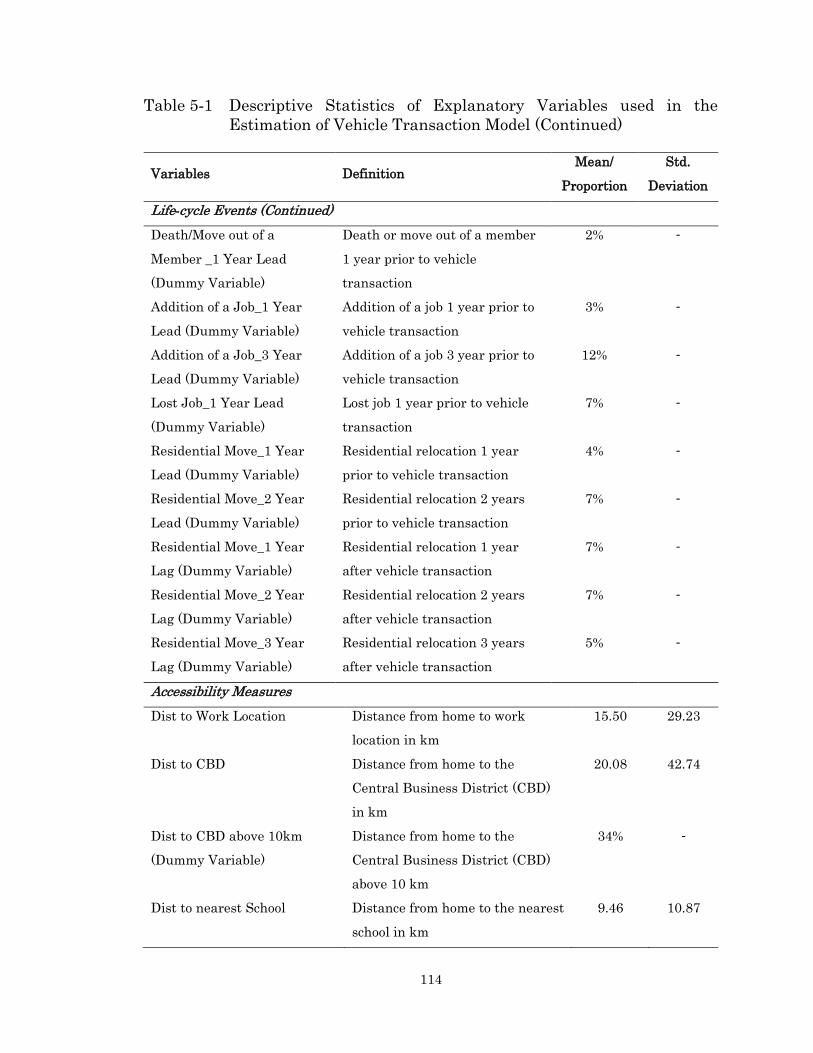
114
Table 5-1 Descriptive Statistics of Explanatory Variables used in the
Estimation of Vehicle Transaction Model (Continued)
Variables Definition Mean/
Proportion
Std.
Deviation
Life-cycle Events (Continued)
Death/Move out of a
Member _1 Year Lead
(Dummy Variable)
Death or move out of a member
1 year prior to vehicle
transaction
2% -
Addition of a Job_1 Year
Lead (Dummy Variable)
Addition of a job 1 year prior to
vehicle transaction
3% -
Addition of a Job_3 Year
Lead (Dummy Variable)
Addition of a job 3 year prior to
vehicle transaction
12% -
Lost Job_1 Year Lead
(Dummy Variable)
Lost job 1 year prior to vehicle
transaction
7% -
Residential Move_1 Year
Lead (Dummy Variable)
Residential relocation 1 year
prior to vehicle transaction
4% -
Residential Move_2 Year
Lead (Dummy Variable)
Residential relocation 2 years
prior to vehicle transaction
7% -
Residential Move_1 Year
Lag (Dummy Variable)
Residential relocation 1 year
after vehicle transaction
7% -
Residential Move_2 Year
Lag (Dummy Variable)
Residential relocation 2 years
after vehicle transaction
7% -
Residential Move_3 Year
Lag (Dummy Variable)
Residential relocation 3 years
after vehicle transaction
5% -
Accessibility Measures
Dist to Work Location Distance from home to work
location in km
15.50 29.23
Dist to CBD Distance from home to the
Central Business District (CBD)
in km
20.08 42.74
Dist to CBD above 10km
(Dummy Variable)
Distance from home to the
Central Business District (CBD)
above 10 km
34% -
Dist to nearest School Distance from home to the nearest
school in km
9.46 10.87

115
Table 5-1 Descriptive Statistics of Explanatory Variables used in the
Estimation of Vehicle Transaction Model (Continued)
Variables Definition Mean/
Proportion
Std.
Deviation
Accessibility Measures (Continued)
Dist to nearest Health Service Distance from home to the nearest
health service in km
6.30 10.82
Dist to nearest Park Area Distance from home to the nearest
park area in km
5.68 29.70
Dist to nearest Park Area
below 1km (Dummy Variable)
Distance from home to the nearest
park area below 1km
87% -
Dist to nearest Shopping
Center
Distance from home to the nearest
shopping center in km
15.07 41.51
Neighbourhood Characteristics
Dwelling Density Dwelling per acre area in the
home dissemination area
1341.43 1802.92
% of Owned Dwelling Percentage of owned dwelling in
the home dissemination area
70.08% 28.81%
% of Single-detached Percentage of single-detached
dwelling in the home
dissemination area
57.86% 33.25%
Avg. Property Value Average property value (CAD) in
the home dissemination area
295242 115095
Employment Rate Employment rate in the home
dissemination area
64.97% 10.64%
In addition to the LSL model, this study develops a multinomial logit (MNL)
model for comparison purposes. The model results suggest that the LSL model
improves the goodness-of-fit measures, as evident in the higher adjusted
pseudo r-squared value (0.26) in comparison to that of the MNL model (0.10).
In terms of log likelihood ratio test, the LSL model yields a chi-squared
statistics of 325.32 (critical value 112.33 with 80 degrees of freedom), which
confirms that the LSL model outperforms the MNL model at the 1%

116
significance level. Hence, this study considers the LSL model as the final
model. The descriptive statistics of the variables retained in the final LSL
model are presented in Table 5-1.
5.3.1 Results of the Segment Allocation Model
The model results of the segment allocation component of the LSL model is
presented in Table 5-2. The results suggest that the segment membership
probabilities for segment one and two are 0.54 and 0.46 respectively. Segment
membership probability is the average probability over the sample households
belonging to each segment.
The segment allocation model is estimated using several socio-demographics
and neighbourhood characteristics. The final segment allocation model retains
the following variables: household income above $100,000, household size,
dwelling density, and percentage of owned dwellings in the neighbourhood
(Table 5-2). The model is estimated assuming segment two as the reference
segment. The model results reveal a negative sign for household size in
segment one, which refers to smaller-sized households. Moreover, membership
of segment one is positively influenced by household income above $100,000.
Among the neighbourhood characteristics, the positive sign for dwelling
density and negative sign for owned dwellings in segment one indicates urban
dwellers. Therefore, segment one can be identified as a segment for smaller-
sized urban dwellers with income above $100,000. On the other hand, segment
two can be identified as a segment for larger-sized suburban dwellers with
income below $100,000.
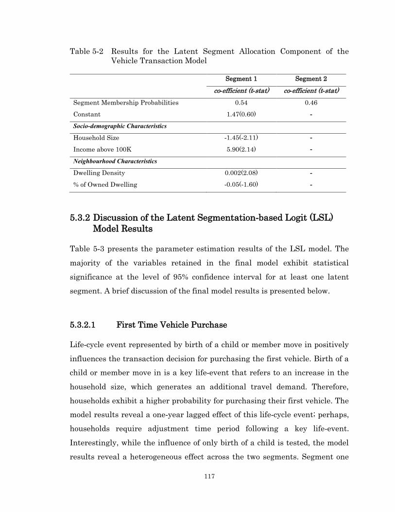
117
Table 5-2 Results for the Latent Segment Allocation Component of the
Vehicle Transaction Model
Segment 1 Segment 2
co-efficient (t-stat) co-efficient (t-stat)
Segment Membership Probabilities 0.54 0.46
Constant 1.47(0.60) -
Socio-demographic Characteristics
Household Size -1.45(-2.11) -
Income above 100K 5.90(2.14) -
Neighbourhood Characteristics
Dwelling Density 0.002(2.08) -
% of Owned Dwelling -0.05(-1.60) -
5.3.2 Discussion of the Latent Segmentation-based Logit (LSL)
Model Results
Table 5-3 presents the parameter estimation results of the LSL model. The
majority of the variables retained in the final model exhibit statistical
significance at the level of 95% confidence interval for at least one latent
segment. A brief discussion of the final model results is presented below.
5.3.2.1 First Time Vehicle Purchase
Life-cycle event represented by birth of a child or member move in positively
influences the transaction decision for purchasing the first vehicle. Birth of a
child or member move in is a key life-event that refers to an increase in the
household size, which generates an additional travel demand. Therefore,
households exhibit a higher probability for purchasing their first vehicle. The
model results reveal a one-year lagged effect of this life-cycle event; perhaps,
households require adjustment time period following a key life-event.
Interestingly, while the influence of only birth of a child is tested, the model
results reveal a heterogeneous effect across the two segments. Segment one

118
identified to include smaller-sized urban dwellers with income above $100,000,
exhibits a higher probability for purchasing the first vehicle. In contrast,
households in segment two reveal a negative relationship. The model confirms
a two-year lagged effect of this variable. Death or move out of a member
referring to a decrease in household size, exhibits a lower probability for
purchasing the first vehicle. Another life-cycle event represented by addition
of a job in the household refers to increased affordability and reveals a
heterogeneous effect across the two segments. Households in segment two
identified as larger-sized suburban dwellers with income below $100,000, show
a higher probability for purchasing their first vehicle. The added budgetary
flexibility due to addition of a job might provide the freedom for purchasing the
first vehicle to these larger-sized suburban dwellers in segment two. In
contrast, households in segment one exhibit a negative relationship. The model
confirms a three-year lagged effect of this variable. Residential relocation
decision reveals a positive relationship in segment two, which is identified to
include larger-sized suburban dwellers with income below $100,000.
Residential relocation might imply a decreased accessibility to activity
locations and transportation services for these larger-sized suburban dwellers,
which triggers the purchase of their first vehicle. On the other hand,
households in segment one reveal a lower probability for purchasing their first
vehicle. The model confirms a one-year lead and a one-year lagged effect of
residential relocation decision.
Among the accessibility and neighbourhood characteristics, households
residing farther away from the closest school locations have a higher
probability for purchasing their first vehicle. A negative relationship is found
for the accessibility measures representing distance to the CBD and distance
to the nearest health services.
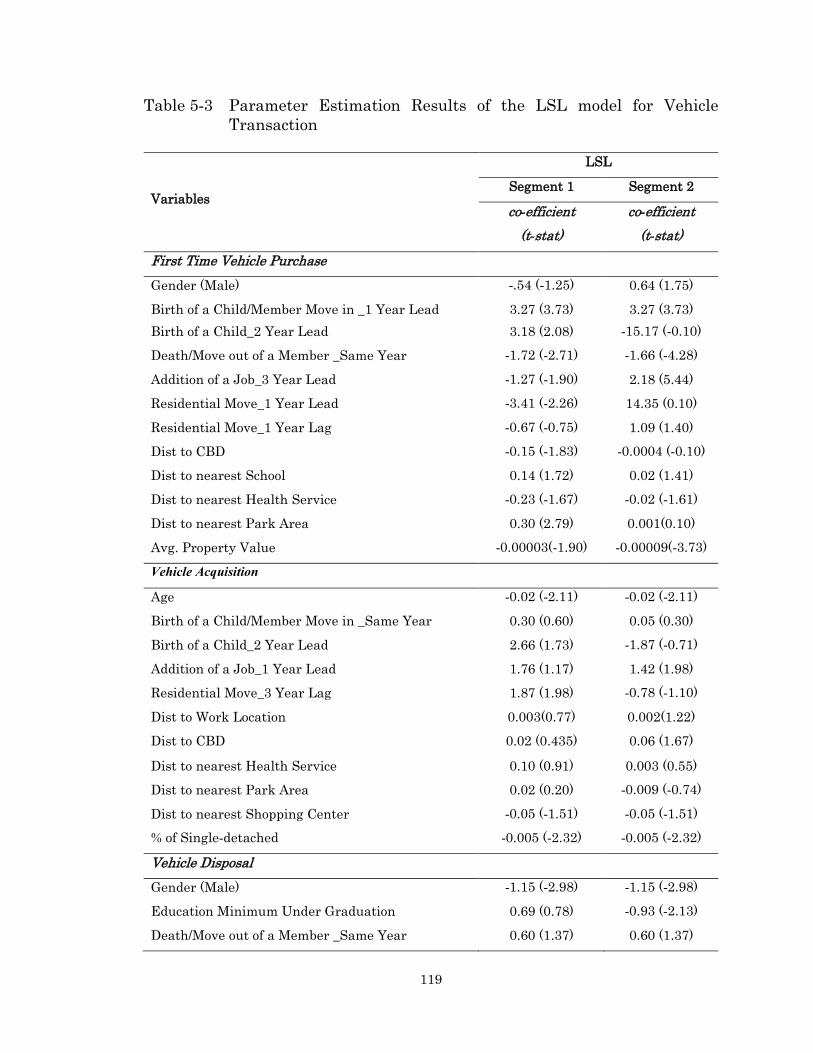
119
Table 5-3 Parameter Estimation Results of the LSL model for Vehicle
Transaction
Variables
LSL
Segment 1 Segment 2
co-efficient
(t-stat)
co-efficient
(t-stat)
First Time Vehicle Purchase
Gender (Male) -.54 (-1.25) 0.64 (1.75)
Birth of a Child/Member Move in _1 Year Lead 3.27 (3.73) 3.27 (3.73)
Birth of a Child_2 Year Lead 3.18 (2.08) -15.17 (-0.10)
Death/Move out of a Member _Same Year -1.72 (-2.71) -1.66 (-4.28)
Addition of a Job_3 Year Lead -1.27 (-1.90) 2.18 (5.44)
Residential Move_1 Year Lead -3.41 (-2.26) 14.35 (0.10)
Residential Move_1 Year Lag -0.67 (-0.75) 1.09 (1.40)
Dist to CBD -0.15 (-1.83) -0.0004 (-0.10)
Dist to nearest School 0.14 (1.72) 0.02 (1.41)
Dist to nearest Health Service -0.23 (-1.67) -0.02 (-1.61)
Dist to nearest Park Area 0.30 (2.79) 0.001(0.10)
Avg. Property Value -0.00003(-1.90) -0.00009(-3.73)
Vehicle Acquisition
Age -0.02 (-2.11) -0.02 (-2.11)
Birth of a Child/Member Move in _Same Year 0.30 (0.60) 0.05 (0.30)
Birth of a Child_2 Year Lead 2.66 (1.73) -1.87 (-0.71)
Addition of a Job_1 Year Lead 1.76 (1.17) 1.42 (1.98)
Residential Move_3 Year Lag 1.87 (1.98) -0.78 (-1.10)
Dist to Work Location 0.003(0.77) 0.002(1.22)
Dist to CBD 0.02 (0.435) 0.06 (1.67)
Dist to nearest Health Service 0.10 (0.91) 0.003 (0.55)
Dist to nearest Park Area 0.02 (0.20) -0.009 (-0.74)
Dist to nearest Shopping Center -0.05 (-1.51) -0.05 (-1.51)
% of Single-detached -0.005 (-2.32) -0.005 (-2.32)
Vehicle Disposal
Gender (Male) -1.15 (-2.98) -1.15 (-2.98)
Education Minimum Under Graduation 0.69 (0.78) -0.93 (-2.13)
Death/Move out of a Member _Same Year 0.60 (1.37) 0.60 (1.37)

120
Table 5-3 Parameter Estimation Results of the LSL model for Vehicle
Transaction (Continued)
Variables
LSL
Segment 1 Segment 2
co-efficient
(t-stat)
co-efficient
(t-stat)
Vehicle Disposal (Continued)
Lost Job_1 Year Lead 0.81 (0.67) 0.84 (1.43)
Residential Move_2 Year Lead 1.27 (2.71) 1.27 (2.71)
Dist to Work Location 0.001 (0.70) 0.001 (0.70)
Dist to nearest Shopping Center 0.06 (1.00) 0.008 (2.23)
% of Single-detached -0.002 (-0.44) -0.002 (-0.44)
Vehicle Trade
Education Minimum Under Graduation 2.80 (2.47) 0.62 (2.04)
Birth of a Child/Member Move in _2 Year Lead 0.94 (1.16) 0.94 (1.16)
Birth of a Child_1 Year Lead 3.93 (2.54) 3.93 (2.54)
Death/Move out of a Member _1 Year Lead 2.86 (1.96) -0.05 (-0.10)
Residential Move_1 Year Lead -3.20 (-1.32) 12.98 (0.10)
Residential Move_2 Year Lag 2.34 (2.14) -11.56 (-0.10)
Dist to CBD above 10km -1.12 (-1.43) 1.55 (5.05)
Dist to nearest Park Area below 1km -0.77 (-0.65) 0.71 (1.99)
Employment Rate 0.04 (2.18) -0.004 (-2.16)
Constants (Reference = Vehicle Disposal)
First Time Vehicle Purchase 5.97 (4.00) 2.47 (2.56)
Vehicle Acquisition 3.10 (2.65) 2.17 (2.69)
Vehicle Trade -2.43 (-1.00) -0.96 (-1.26)
Goodness-of-fit Measures
Log Likelihood (at convergence) -453.50
Log Likelihood (at constant) -616.16
Adjusted Pseudo R-squared 0.26
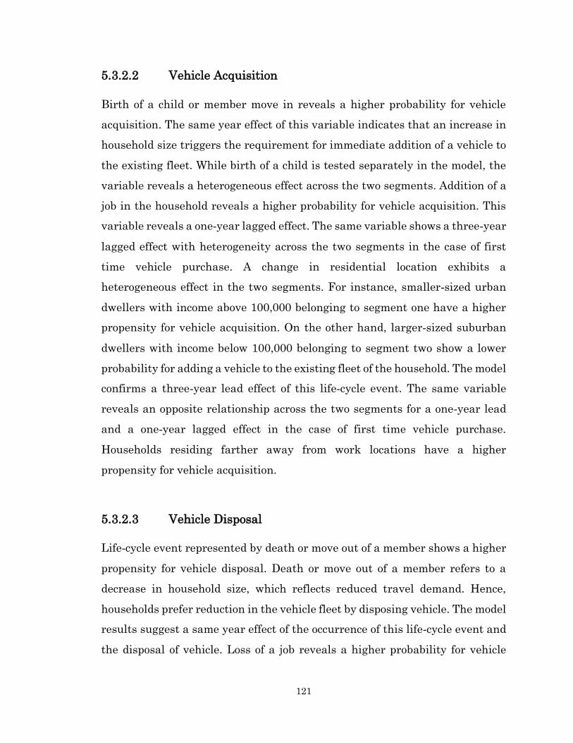
121
5.3.2.2 Vehicle Acquisition
Birth of a child or member move in reveals a higher probability for vehicle
acquisition. The same year effect of this variable indicates that an increase in
household size triggers the requirement for immediate addition of a vehicle to
the existing fleet. While birth of a child is tested separately in the model, the
variable reveals a heterogeneous effect across the two segments. Addition of a
job in the household reveals a higher probability for vehicle acquisition. This
variable reveals a one-year lagged effect. The same variable shows a three-year
lagged effect with heterogeneity across the two segments in the case of first
time vehicle purchase. A change in residential location exhibits a
heterogeneous effect in the two segments. For instance, smaller-sized urban
dwellers with income above 100,000 belonging to segment one have a higher
propensity for vehicle acquisition. On the other hand, larger-sized suburban
dwellers with income below 100,000 belonging to segment two show a lower
probability for adding a vehicle to the existing fleet of the household. The model
confirms a three-year lead effect of this life-cycle event. The same variable
reveals an opposite relationship across the two segments for a one-year lead
and a one-year lagged effect in the case of first time vehicle purchase.
Households residing farther away from work locations have a higher
propensity for vehicle acquisition.
5.3.2.3 Vehicle Disposal
Life-cycle event represented by death or move out of a member shows a higher
propensity for vehicle disposal. Death or move out of a member refers to a
decrease in household size, which reflects reduced travel demand. Hence,
households prefer reduction in the vehicle fleet by disposing vehicle. The model
results suggest a same year effect of the occurrence of this life-cycle event and
the disposal of vehicle. Loss of a job reveals a higher probability for vehicle
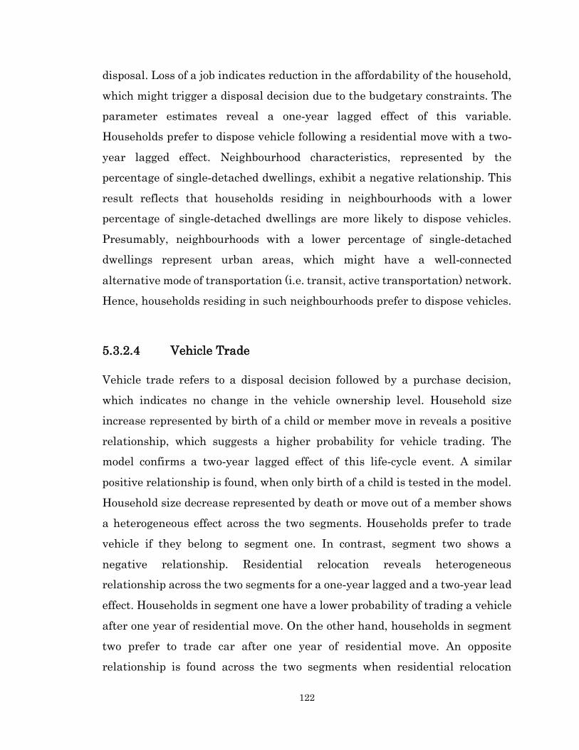
122
disposal. Loss of a job indicates reduction in the affordability of the household,
which might trigger a disposal decision due to the budgetary constraints. The
parameter estimates reveal a one-year lagged effect of this variable.
Households prefer to dispose vehicle following a residential move with a two-
year lagged effect. Neighbourhood characteristics, represented by the
percentage of single-detached dwellings, exhibit a negative relationship. This
result reflects that households residing in neighbourhoods with a lower
percentage of single-detached dwellings are more likely to dispose vehicles.
Presumably, neighbourhoods with a lower percentage of single-detached
dwellings represent urban areas, which might have a well-connected
alternative mode of transportation (i.e. transit, active transportation) network.
Hence, households residing in such neighbourhoods prefer to dispose vehicles.
5.3.2.4 Vehicle Trade
Vehicle trade refers to a disposal decision followed by a purchase decision,
which indicates no change in the vehicle ownership level. Household size
increase represented by birth of a child or member move in reveals a positive
relationship, which suggests a higher probability for vehicle trading. The
model confirms a two-year lagged effect of this life-cycle event. A similar
positive relationship is found, when only birth of a child is tested in the model.
Household size decrease represented by death or move out of a member shows
a heterogeneous effect across the two segments. Households prefer to trade
vehicle if they belong to segment one. In contrast, segment two shows a
negative relationship. Residential relocation reveals heterogeneous
relationship across the two segments for a one-year lagged and a two-year lead
effect. Households in segment one have a lower probability of trading a vehicle
after one year of residential move. On the other hand, households in segment
two prefer to trade car after one year of residential move. An opposite
relationship is found across the two segments when residential relocation
123
decision is examined for a two-year lead effect. Accessibility measures
represented by distance to the CBD above 10km and distance to the nearest
park area below 1km indicate heterogeneous relationships across the two
segments.
In addition to the above mentioned variables retained in the final model, this
study tests a number of variables during the model estimation process. For
instance, the study tests the effects of retirement, job move, distance from
home to the nearest transit station, dwelling type, and percentage of different
land uses in the neighbourhood, among others. Moreover, the study tests a
number of variables to estimate the latent segment allocation model, such as
presence of children, percentage of rented dwellings in the neighbourhood, and
land-use mix index, among others. However, the above mentioned variables
could not be included in the final model due to discrepancies in the hypotheses
confirmation along with poor statistical significance. Additionally, the final
model includes some variables below the level of 95% confidence interval as
they offer important behavioural insights and have significant policy
implications. These variables are retained with an assumption that they might
show statistical significance if a larger dataset were available.
5.4 Conclusions and Summary of Contributions
This research presents the findings of a dynamic household-level vehicle
transaction model. A latent segmentation-based logit (LSL) model is developed
to investigate four types of transaction decisions, including first time vehicle
purchase, vehicle acquisition, vehicle disposal, and vehicle trade. One of the
unique features of this study is to identify the transaction decision of the first
time vehicle purchase. The LSL model captures repeated transactions of the
same households during their life-course. A segment allocation model is
formulated within the LSL framework to address latent heterogeneity. The
124
allocation of households into different latent segments is estimated on the
basis of household income, household size, dwelling density of the
neighbourhood, and percentage of owned dwelling in the neighbourhood. This
study tests the lead and lagged effects of life-cycle events. The model results
suggest that considerable heterogeneity exists, as evident in the parametric
values of two latent segments. For instance, addition of a job could trigger first
time vehicle purchase in one segment and deter in another segment. Similar
heterogeneous effect is found for the variable representing birth of a child for
vehicle acquisition. The effect of historical deposition is also confirmed on
vehicle transaction decisions. For example, birth of a child confirms a two-year
lagged effect on vehicle acquisition. Interestingly, the first time vehicle
purchase behaviour is found to be considerably different than vehicle
acquisition decisions (addition of a vehicle to the existing vehicle fleet). For
instance, addition of a job reveals significant heterogeneity across the two
segments in the case of first time vehicle purchase. The model confirms that
households require three years of adjustment period after getting a job to
purchase their first vehicle. The same variable exhibits a higher probability for
vehicle acquisition in both segments, and confirms a smaller adjustment period
of one year. Additionally, the model confirms a one-year lead and a one-year
lagged effect of residential move for first time vehicle purchase decisions,
which exhibit heterogeneity across the two segments. On the other hand, the
same variable shows an opposite relationship across the two segments for
vehicle acquisition decision with a three-year lead effect.
One of the limitations of this study is that it could not consider the historical
evolution of the transportation system. As a result, the effects of certain
variables including transit availability, transit level of service (LOS), travel
time, and travel cost, among others could not be addressed in the model. A
travel demand forecasting model for Halifax is currently under development,
which is expected to provide better information regarding travel time, transit
125
LOS, and other relevant information for further modelling. Another limitation
is the use of a small sample size. Particularly, analyzing different domains of
contrasts with respect to multiple choice dimensions and latent segmentation
are challenging with a small sample size. If larger sample becomes available,
one interesting future direction could be testing genearational effects and other
influences of time-varying factors. One of the future directions in the domain
of model development is to consider car availability constraints during choice
set formulation for the transaction instances, which might improve the model
estimation results. In addition, future studies should focus on developing a
latent segmentation-based nested logit modelling framework to capture
endogeneity within the decision process.
In summary, this study contributes significantly towards the vehicle
ownership literature by developing a life-oriented vehicle transaction model.
The model disentangles a crucial behaviour regarding first time vehicle
purchase decisions of the households. The study examines lead and lagged
effects of life-cycle events. The historical deposition effects of the key life-events
found in this study offer important behavioural insights in understanding
vehicle transaction decisions. It will be interesting to microsimulate this
dynamic vehicle transaction model within the iTLE framework.
126
Chapter 6
6 Baseline Synthesis and
Microsimulation of Life-stage
Transitions
6.1 Introduction
This chapter presents the implementation of the baseline synthesis and life-
stage transition modules of the life-oriented integrated Transport Land Use
and Energy (iTLE) model. Baseline synthesis involves the generation of
relevant baseline information of the agents such as demographic and vehicle
ownership information. Life-stage transition includes the simulation of the
demographic career of the agents. The contributions of this research is three-
fold: 1) performing population synthesis at the micro-spatial resolution of
parcel, 2) synthesizing vehicle ownership level, and 3) microsimulating the life-
stages of the agents. A full-scale validation of the baseline synthesis and life-
stage transition simulation results are also performed.
This chapter is organized as follows: section 6.2 discusses the implementation
of the iTLE model. Section 6.3 presents population synthesis process and
results. Section 6.4 describes the vehicle ownership level synthesis. Section 6.5
discusses the implementation of the life-stage transition module, including the
microsimulation processes, validation, and simulation results. The chapter
concludes with a summary of contributions in section 6.6.
The following journal paper is an earlier version of this chapter:
Fatmi, M.R., and Habib, M.A. (2017). Baseline Synthesis and Microsimulation of Life-
stage Transitions within an Agent-based Integrated Urban Model. Procedia Computer Science, 109, 608-315.
127
6.2 Implementation of the iTLE Proto-type Model
A proto-type version of the iTLE model is operationalized for Halifax, Canada.
The proto-type version implements the following modules: baseline synthesis,
life-stage transition, residential location transition, and vehicle ownership
transition. The program code is written using C# dotNET programming
language. The iTLE proto-type contains a total of approximately 1700 lines of
code. The proto-type version generates baseline synthetic information for the
year 2006, and runs simulation for a 15-year period from 2007 to 2021 at a
yearly time-step. The run-time of the model for each simulation year is around
23 hours on a computer with Core i7-4770 processor and 16 GB of RAM,
running on a 64-bit Windows 7 operating system.
The proto-type iTLE simulates agents’ decisions longitudinally at each
simulation year. The simulation starts with a sample of baseline population,
and the relationships among the agents in the population are maintained
throughout the simulation period. An agent can enter the population through
birth or in-migration and exit through death or out-migration. The system
state of iTLE does not hold the equilibrium assumption, rather it is always in
a dynamic dis-equilibrium state. iTLE is designed as a modular-based
modelling system, which allows the application of each module and subsequent
micro-models in isolation and offers the opportunity to improve any component
without affecting the whole simulation framework. All urban form elements
are considered as exogenous in the current version of iTLE software. Following
the simulation at each time-step, the system output is stored at the individual
agent- and object-level; which can be used to generate numerous statistics and
maps at different aggregation levels. This chapter presents the results of
population synthesis, vehicle ownership level synthesis, and life-stage
transition components of the iTLE model.

128
6.3 Population Synthesis
6.3.1 Synthesis Process
The population for the base year is generated in the following two-stages: (1)
generation of synthetic population at the zonal-level, and (2) allocation of the
synthetic population at the micro-spatial unit of parcel. The first stage involves
synthesizing the population at the zonal-level of dissemination area (DA). A
100% synthetic population is generated following an Iterative Proportional
Updating (IPU) technique (Ye et al., 2009) for the base year 2006. In the IPU
technique, control for both household-level and individual-level characteristics
is maintained by adjusting weights iteratively among the attribute types of the
households until attribute types at the household- and individual-level are
matched. The synthesis is performed using an open source population
synthesizer, PopGen. For the synthesis, the household-level control variables
include, household income, household size, tenure type, and dwelling type; and
the individual-level control variables include, age, sex, marital status, and
employment status. A list of categories for the household-level and individual-
level control variables are presented in Table 6-1.
The iTLE model is designed to operate at the finest disaggregate spatial unit
of parcel. Hence, the second stage involves allocation of the households into the
parcels using a logit link model. To control the allocation of the households into
parcels of the DA it belongs (according to stage one), a constraint is introduced
in the logit link model. This constraint generates household-specific choice set,
which only includes the parcels of the specific DA that the household is
allocated through synthesis. A multinomial logit model (MNL) is developed to
generate the initial parcel-level residential locations (Table 6-2). The allocation
of households into the parcels is determined based on parcel characteristics
and its interaction with households’ socio-economic characteristics.
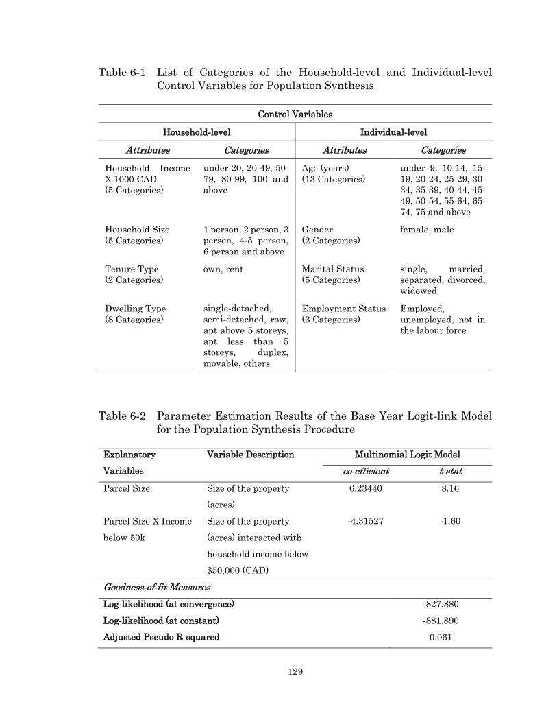
129
Table 6-1 List of Categories of the Household-level and Individual-level
Control Variables for Population Synthesis
Control Variables
Household-level Individual-level
Attributes Categories Attributes Categories
Household Income
X 1000 CAD
(5 Categories)
under 20, 20-49, 50-
79, 80-99, 100 and
above
Age (years)
(13 Categories)
under 9, 10-14, 15-
19, 20-24, 25-29, 30-
34, 35-39, 40-44, 45-
49, 50-54, 55-64, 65-
74, 75 and above
Household Size
(5 Categories)
1 person, 2 person, 3
person, 4-5 person,
6 person and above
Gender
(2 Categories)
female, male
Tenure Type
(2 Categories)
own, rent Marital Status
(5 Categories)
single, married,
separated, divorced,
widowed
Dwelling Type
(8 Categories)
single-detached,
semi-detached, row,
apt above 5 storeys,
apt less than 5
storeys, duplex,
movable, others
Employment Status
(3 Categories)
Employed,
unemployed, not in
the labour force
Table 6-2 Parameter Estimation Results of the Base Year Logit-link Model
for the Population Synthesis Procedure
Explanatory
Variables
Variable Description Multinomial Logit Model
co-efficient t-stat
Parcel Size Size of the property
(acres)
6.23440 8.16
Parcel Size X Income
below 50k
Size of the property
(acres) interacted with
household income below
$50,000 (CAD)
-4.31527 -1.60
Goodness-of-fit Measures
Log-likelihood (at convergence) -827.880
Log-likelihood (at constant) -881.890
Adjusted Pseudo R-squared 0.061
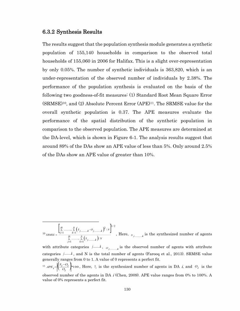
130
6.3.2 Synthesis Results
The results suggest that the population synthesis module generates a synthetic
population of 155,140 households in comparison to the observed total
households of 155,060 in 2006 for Halifax. This is a slight over-representation
by only 0.05%. The number of synthetic individuals is 363,820, which is an
under-representation of the observed number of individuals by 2.38%. The
performance of the population synthesis is evaluated on the basis of the
following two goodness-of-fit measures: (1) Standard Root Mean Square Error
(SRMSE)10, and (2) Absolute Percent Error (APE)11. The SRMSE value for the
overall synthetic population is 0.37. The APE measures evaluate the
performance of the spatial distribution of the synthetic population in
comparison to the observed population. The APE measures are determined at
the DA-level, which is shown in Figure 6-1. The analysis results suggest that
around 89% of the DAs show an APE value of less than 5%. Only around 2.5%
of the DAs show an APE value of greater than 10%.
10
2/1
1 1
/..........
............
1 1
/2
................................
m
j
n
k
Nkj
S
m
j
n
k
Nkj
Okj
S
SRMSE , Here, kjS ..........
is the synthesized number of agents
with attribute categories kj.......... , kjO ..........
is the observed number of agents with attribute
categories kj.......... , and N is the total number of agents (Farooq et al., 2013). SRMSE value
generally ranges from 0 to 1. A value of 0 represents a perfect fit.
11 100*
iO
iO
iS
iAPE
, Here, iS is the synthesized number of agents in DA i, and iO is the
observed number of the agents in DA i (Chen, 2009). APE value ranges from 0% to 100%. A
value of 0% represents a perfect fit.
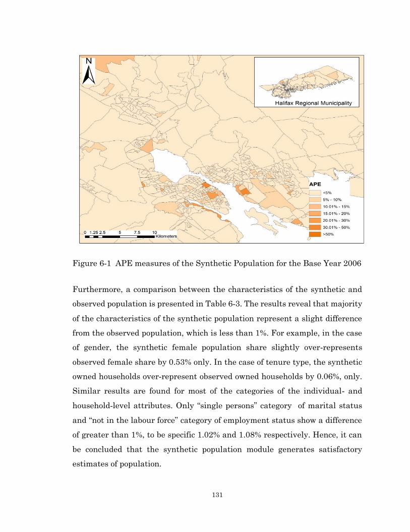
131
Figure 6-1 APE measures of the Synthetic Population for the Base Year 2006
Furthermore, a comparison between the characteristics of the synthetic and
observed population is presented in Table 6-3. The results reveal that majority
of the characteristics of the synthetic population represent a slight difference
from the observed population, which is less than 1%. For example, in the case
of gender, the synthetic female population share slightly over-represents
observed female share by 0.53% only. In the case of tenure type, the synthetic
owned households over-represent observed owned households by 0.06%, only.
Similar results are found for most of the categories of the individual- and
household-level attributes. Only “single persons” category of marital status
and “not in the labour force” category of employment status show a difference
of greater than 1%, to be specific 1.02% and 1.08% respectively. Hence, it can
be concluded that the synthetic population module generates satisfactory
estimates of population.
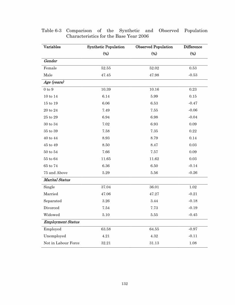
132
Table 6-3 Comparison of the Synthetic and Observed Population
Characteristics for the Base Year 2006
Variables Synthetic Population
(%)
Observed Population
(%)
Difference
(%)
Gender
Female 52.55 52.02 0.53
Male 47.45 47.98 -0.53
Age (years)
0 to 9 10.39 10.16 0.23
10 to 14 6.14 5.99 0.15
15 to 19 6.06 6.53 -0.47
20 to 24 7.49 7.55 -0.06
25 to 29 6.94 6.98 -0.04
30 to 34 7.02 6.93 0.09
35 to 39 7.58 7.35 0.22
40 to 44 8.93 8.79 0.14
45 to 49 8.50 8.47 0.03
50 to 54 7.66 7.57 0.09
55 to 64 11.65 11.62 0.03
65 to 74 6.36 6.50 -0.14
75 and Above 5.29 5.56 -0.26
Marital Status
Single 37.04 36.01 1.02
Married 47.06 47.27 -0.21
Separated 3.26 3.44 -0.18
Divorced 7.54 7.73 -0.19
Widowed 5.10 5.55 -0.45
Employment Status
Employed 63.58 64.55 -0.97
Unemployed 4.21 4.32 -0.11
Not in Labour Force 32.21 31.13 1.08

133
Table 6-3 Comparison of the Synthetic and Observed Population
Characteristics for the Base Year 2006 (Continued)
Variables Synthetic
Population (%)
Observed
Population (%)
Difference
(%)
Household Size
1 person 27.76 27.74 0.03
2 person 35.57 35.56 0.00
3 person 16.67 16.65 0.02
4-5 person 18.54 18.51 0.03
6 person and Above 1.46 1.54 -0.07
Household Income (1000 $CAD)
Under 20 15.31 15.36 -0.04
20 to 49 30.90 30.96 -0.06
50 to 79 24.11 24.06 0.05
80 to 99 10.89 10.97 -0.08
100 and Above 18.79 18.65 0.14
Tenure Type
Own 64.07 64.01 0.06
Rent 35.93 35.99 -0.06
Dwelling Type
Single-detached 51.52 51.57 -0.05
Semi-detached 6.74 6.81 -0.07
Row House 3.51 3.51 0.00
Apartment with 5 and Above
Storey 9.59 9.53 0.06
Apartment with Less than 5
Storey 22.15 22.09 0.06
Duplex Apartment 4.04 4.04 0.01
Movable 2.26 2.28 -0.02
Other 0.19 0.19 0.01
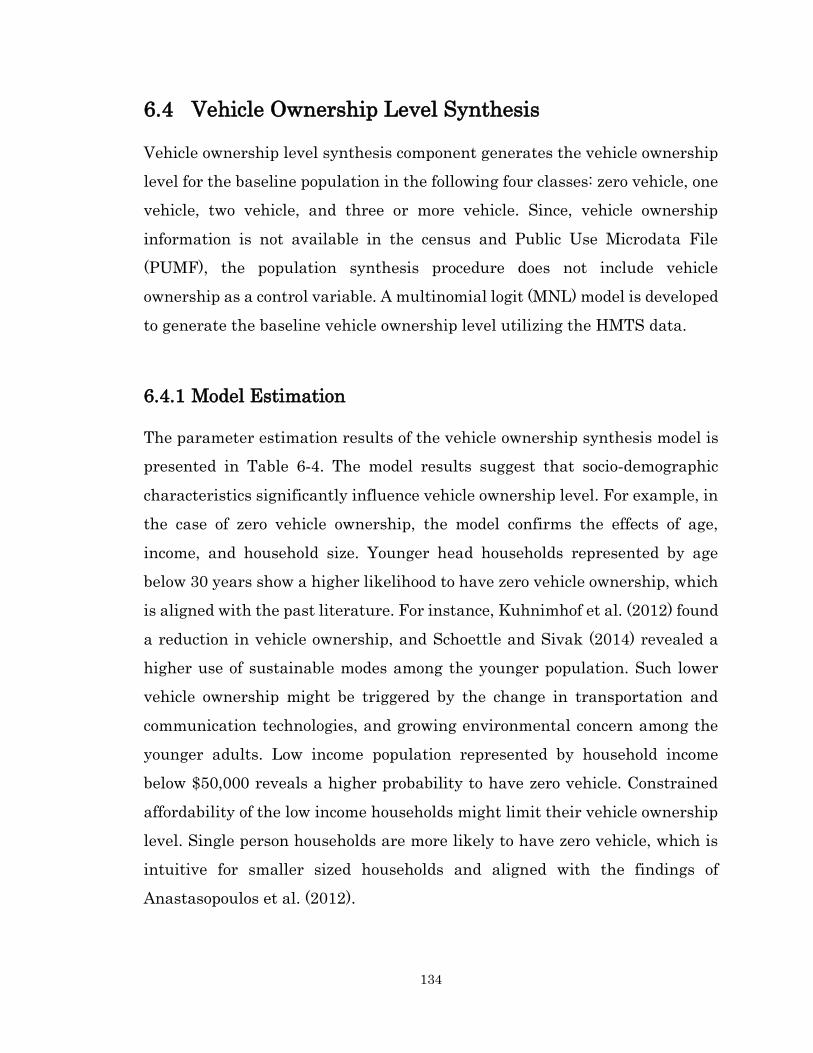
134
6.4 Vehicle Ownership Level Synthesis
Vehicle ownership level synthesis component generates the vehicle ownership
level for the baseline population in the following four classes: zero vehicle, one
vehicle, two vehicle, and three or more vehicle. Since, vehicle ownership
information is not available in the census and Public Use Microdata File
(PUMF), the population synthesis procedure does not include vehicle
ownership as a control variable. A multinomial logit (MNL) model is developed
to generate the baseline vehicle ownership level utilizing the HMTS data.
6.4.1 Model Estimation
The parameter estimation results of the vehicle ownership synthesis model is
presented in Table 6-4. The model results suggest that socio-demographic
characteristics significantly influence vehicle ownership level. For example, in
the case of zero vehicle ownership, the model confirms the effects of age,
income, and household size. Younger head households represented by age
below 30 years show a higher likelihood to have zero vehicle ownership, which
is aligned with the past literature. For instance, Kuhnimhof et al. (2012) found
a reduction in vehicle ownership, and Schoettle and Sivak (2014) revealed a
higher use of sustainable modes among the younger population. Such lower
vehicle ownership might be triggered by the change in transportation and
communication technologies, and growing environmental concern among the
younger adults. Low income population represented by household income
below $50,000 reveals a higher probability to have zero vehicle. Constrained
affordability of the low income households might limit their vehicle ownership
level. Single person households are more likely to have zero vehicle, which is
intuitive for smaller sized households and aligned with the findings of
Anastasopoulos et al. (2012).
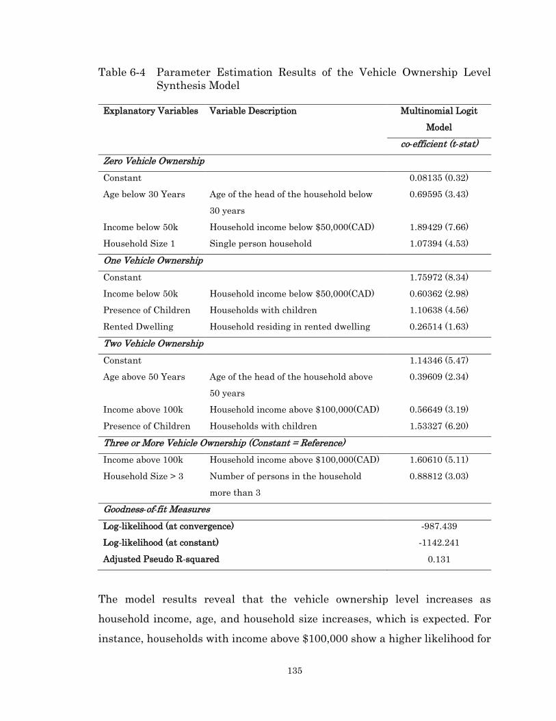
135
Table 6-4 Parameter Estimation Results of the Vehicle Ownership Level
Synthesis Model
Explanatory Variables Variable Description Multinomial Logit
Model
co-efficient (t-stat)
Zero Vehicle Ownership
Constant 0.08135 (0.32)
Age below 30 Years
Age of the head of the household below
30 years
0.69595 (3.43)
Income below 50k Household income below $50,000(CAD) 1.89429 (7.66)
Household Size 1 Single person household 1.07394 (4.53)
One Vehicle Ownership
Constant 1.75972 (8.34)
Income below 50k Household income below $50,000(CAD) 0.60362 (2.98)
Presence of Children Households with children 1.10638 (4.56)
Rented Dwelling Household residing in rented dwelling 0.26514 (1.63)
Two Vehicle Ownership
Constant 1.14346 (5.47)
Age above 50 Years
Age of the head of the household above
50 years
0.39609 (2.34)
Income above 100k Household income above $100,000(CAD) 0.56649 (3.19)
Presence of Children Households with children 1.53327 (6.20)
Three or More Vehicle Ownership (Constant = Reference)
Income above 100k Household income above $100,000(CAD) 1.60610 (5.11)
Household Size > 3 Number of persons in the household
more than 3
0.88812 (3.03)
Goodness-of-fit Measures
Log-likelihood (at convergence) -987.439
Log-likelihood (at constant) -1142.241
Adjusted Pseudo R-squared 0.131
The model results reveal that the vehicle ownership level increases as
household income, age, and household size increases, which is expected. For
instance, households with income above $100,000 show a higher likelihood for

136
two vehicle ownership. In the case of three or more vehicles, the effect of the
same variable representing income above $100,000 increases by 3 times. Older
head households with age above 50 years show a positive association with two
vehicle ownership; since, older population of this generation are more
dependent on cars and prefer higher vehicle ownership (Hjorthol et al., 2010).
Interestingly, presence of children in the household show a positive
relationship for one vehicle ownership and two vehicle ownership. Arguably,
individuals with children might require to trip chain to day care
centers/schools on their way to work, and require car for convenience. This
variable shows a 1.5 times stronger relationship for two vehicle ownership than
one, which is expected as multiple vehicles might offer added flexibility to both
the parents or other members of the household to travel with children. All the
variables retained in the final model exhibit statistical significance at the level
of 95% confidence interval.
6.4.2 Vehicle Ownership Level Synthesis Results
The MNL model described above is utilized to determine the probability of a
household to own zero, one, two, and three or more vehicles. Households are
assigned to a vehicle ownership level following the order of probability
estimation. The distribution of the generated baseline vehicle ownership level
for 2006 is illustrated in Figure 6-2. The results suggest that 22.55% of the
households do not own a vehicle, 37.40% own one vehicle, 32.16% own two
vehicles, and 7.89% own three or more vehicles. Due to the unavailability of
the actual vehicle ownership information in 2006 for Halifax, the results could
not be validated.

137
Figure 6-2 Vehicle Ownership Level Synthesis Results for the Year 2006
6.5 Population Life-stage Transition Module
6.5.1 Microsimulation Process
The current version of iTLE simulates the following six life-stage transitions:
ageing, death, birth, out-migration, in-migration, and household formation.
The proto-type implements this module at a yearly time-step for the simulation
years 2007 to 2021. A 10% sample of the synthesized Halifax population is used
for the simulation.
The life-stage transitions are simulated as binary probabilities of a transition
to occur or not. This module follows a heuristic modelling approaches, where
average of the historical rates (Appendix A) are used to determine the rate of
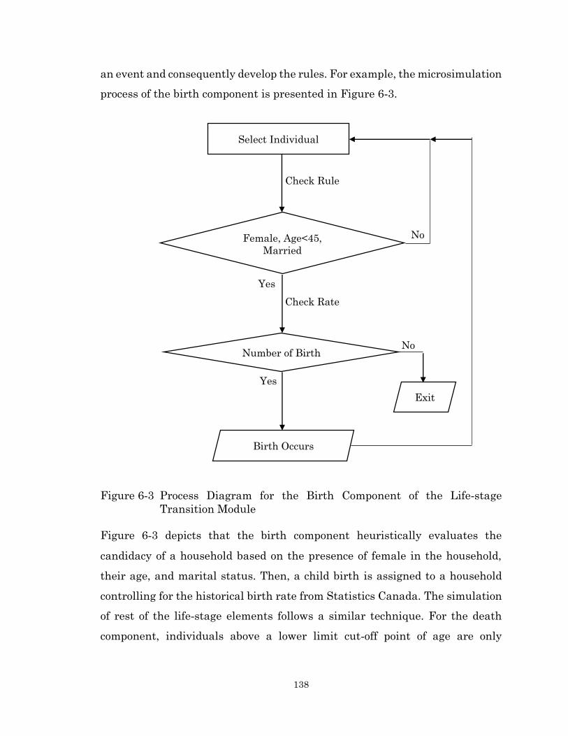
138
an event and consequently develop the rules. For example, the microsimulation
process of the birth component is presented in Figure 6-3.
Figure 6-3 Process Diagram for the Birth Component of the Life-stage
Transition Module
Figure 6-3 depicts that the birth component heuristically evaluates the
candidacy of a household based on the presence of female in the household,
their age, and marital status. Then, a child birth is assigned to a household
controlling for the historical birth rate from Statistics Canada. The simulation
of rest of the life-stage elements follows a similar technique. For the death
component, individuals above a lower limit cut-off point of age are only
Select Individual
Female, Age<45,
Married
Number of Birth
Birth Occurs
Exit
Check Rule
Check Rate
No
Yes
Yes
No
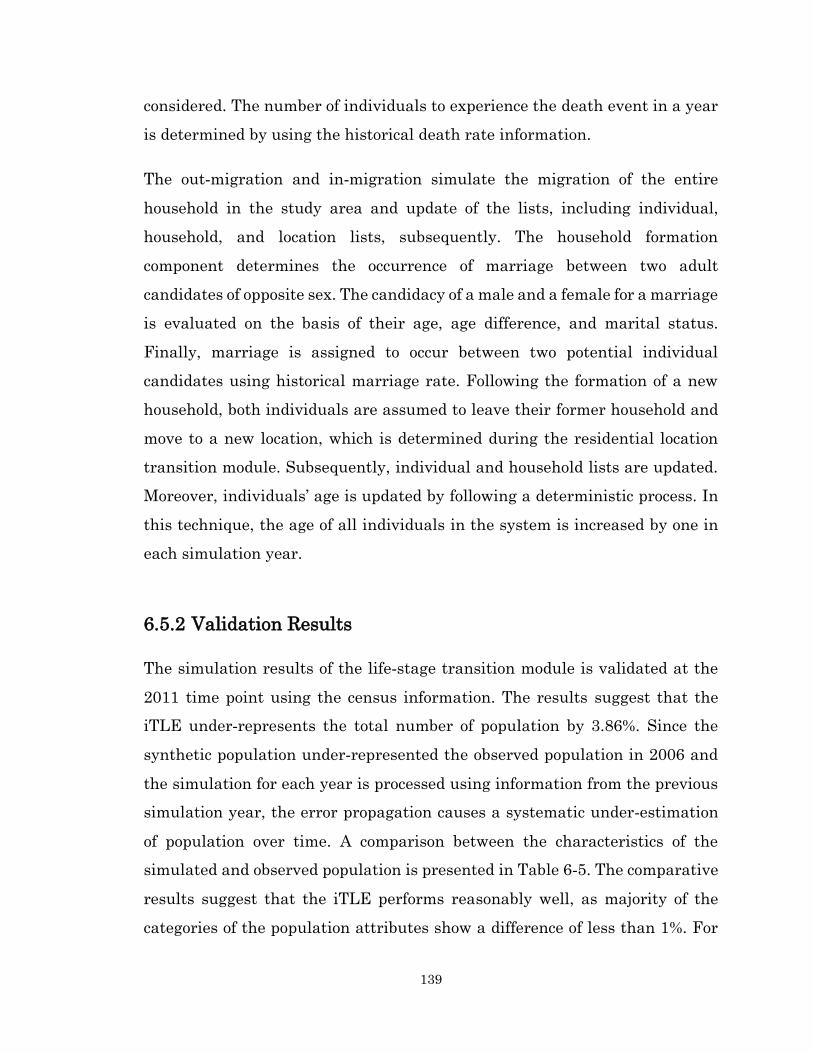
139
considered. The number of individuals to experience the death event in a year
is determined by using the historical death rate information.
The out-migration and in-migration simulate the migration of the entire
household in the study area and update of the lists, including individual,
household, and location lists, subsequently. The household formation
component determines the occurrence of marriage between two adult
candidates of opposite sex. The candidacy of a male and a female for a marriage
is evaluated on the basis of their age, age difference, and marital status.
Finally, marriage is assigned to occur between two potential individual
candidates using historical marriage rate. Following the formation of a new
household, both individuals are assumed to leave their former household and
move to a new location, which is determined during the residential location
transition module. Subsequently, individual and household lists are updated.
Moreover, individuals’ age is updated by following a deterministic process. In
this technique, the age of all individuals in the system is increased by one in
each simulation year.
6.5.2 Validation Results
The simulation results of the life-stage transition module is validated at the
2011 time point using the census information. The results suggest that the
iTLE under-represents the total number of population by 3.86%. Since the
synthetic population under-represented the observed population in 2006 and
the simulation for each year is processed using information from the previous
simulation year, the error propagation causes a systematic under-estimation
of population over time. A comparison between the characteristics of the
simulated and observed population is presented in Table 6-5. The comparative
results suggest that the iTLE performs reasonably well, as majority of the
categories of the population attributes show a difference of less than 1%. For

140
example, in the case of marital status, the simulated single population share
slightly under-represents observed single population by 0.40% only.
Table 6-5 Comparison of Simulated and Observed Population Characteristics
for the Year 2011
Variables Simulated Population (%) Observed Population (%) Difference (%)
Gender
Female 52.77 51.65 1.12
Male 47.23 48.35 -1.12
Age (years)
0 to 9 5.51 10.03 -4.52
10 to 14 10.24 5.25 4.99
15 to 19 5.90 6.11 -0.21
20 to 24 5.63 8.01 -2.38
25 to 29 7.50 7.29 0.21
30 to 34 7.37 6.68 0.69
35 to 39 7.10 6.79 0.31
40 to 44 7.18 7.14 0.04
45 to 49 8.68 8.49 0.19
50 to 54 7.87 8.11 -0.24
55 to 64 6.68 13.14 -6.46
65 to 74 10.27 7.30 2.97
75 and Above 10.06 5.64 4.42
Marital Status
Single 39.92 40.32 -0.40
Married 45.77 45.95 -0.18
Separated 2.98 2.83 0.15
Divorced 6.95 5.91 1.04
Widowed 4.39 5.00 -0.61
Household Size
1 person 29.19 28.56 0.63
2 person 34.26 36.50 -2.24
3 person 15.61 16.35 -0.74
4-5 person 18.25 17.06 1.19
6 person and Above 2.70 1.54 1.16
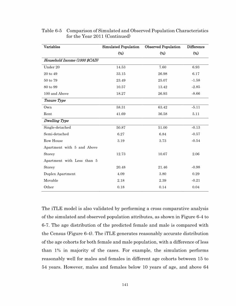
141
Table 6-5 Comparison of Simulated and Observed Population Characteristics
for the Year 2011 (Continued)
Variables Simulated Population
(%)
Observed Population
(%)
Difference
(%)
Household Income (1000 $CAD)
Under 20 14.53 7.60 6.93
20 to 49 33.15 26.98 6.17
50 to 79 23.49 25.07 -1.58
80 to 99 10.57 13.42 -2.85
100 and Above 18.27 26.93 -8.66
Tenure Type
Own 58.31 63.42 -5.11
Rent 41.69 36.58 5.11
Dwelling Type
Single-detached 50.87 51.00 -0.13
Semi-detached 6.27 6.84 -0.57
Row House 3.19 3.73 -0.54
Apartment with 5 and Above
Storey 12.73 10.67 2.06
Apartment with Less than 5
Storey 20.48 21.46 -0.98
Duplex Apartment 4.09 3.80 0.29
Movable 2.18 2.39 -0.21
Other 0.18 0.14 0.04
The iTLE model is also validated by performing a cross comparative analysis
of the simulated and observed population attributes, as shown in Figure 6-4 to
6-7. The age distribution of the predicted female and male is compared with
the Census (Figure 6-4). The iTLE generates reasonably accurate distribution
of the age cohorts for both female and male population, with a difference of less
than 1% in majority of the cases. For example, the simulation performs
reasonably well for males and females in different age cohorts between 15 to
54 years. However, males and females below 10 years of age, and above 64
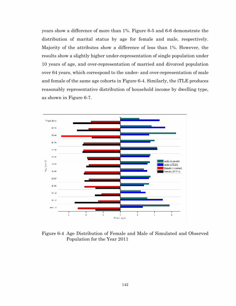
142
years show a difference of more than 1%. Figure 6-5 and 6-6 demonstrate the
distribution of marital status by age for female and male, respectively.
Majority of the attributes show a difference of less than 1%. However, the
results show a slightly higher under-representation of single population under
10 years of age, and over-representation of married and divorced population
over 64 years, which correspond to the under- and over-representation of male
and female of the same age cohorts in Figure 6-4. Similarly, the iTLE produces
reasonably representative distribution of household income by dwelling type,
as shown in Figure 6-7.
Figure 6-4 Age Distribution of Female and Male of Simulated and Observed
Population for the Year 2011
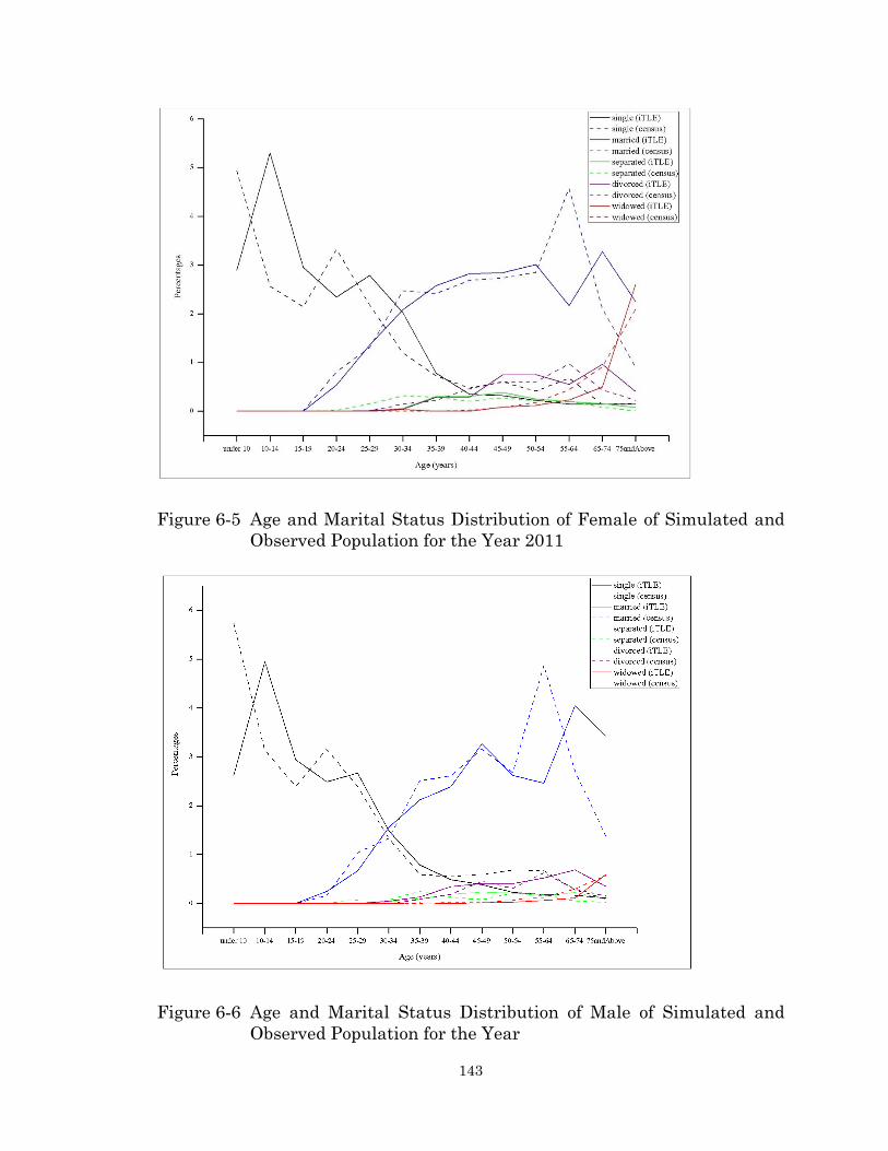
143
Figure 6-5 Age and Marital Status Distribution of Female of Simulated and
Observed Population for the Year 2011
Figure 6-6 Age and Marital Status Distribution of Male of Simulated and
Observed Population for the Year
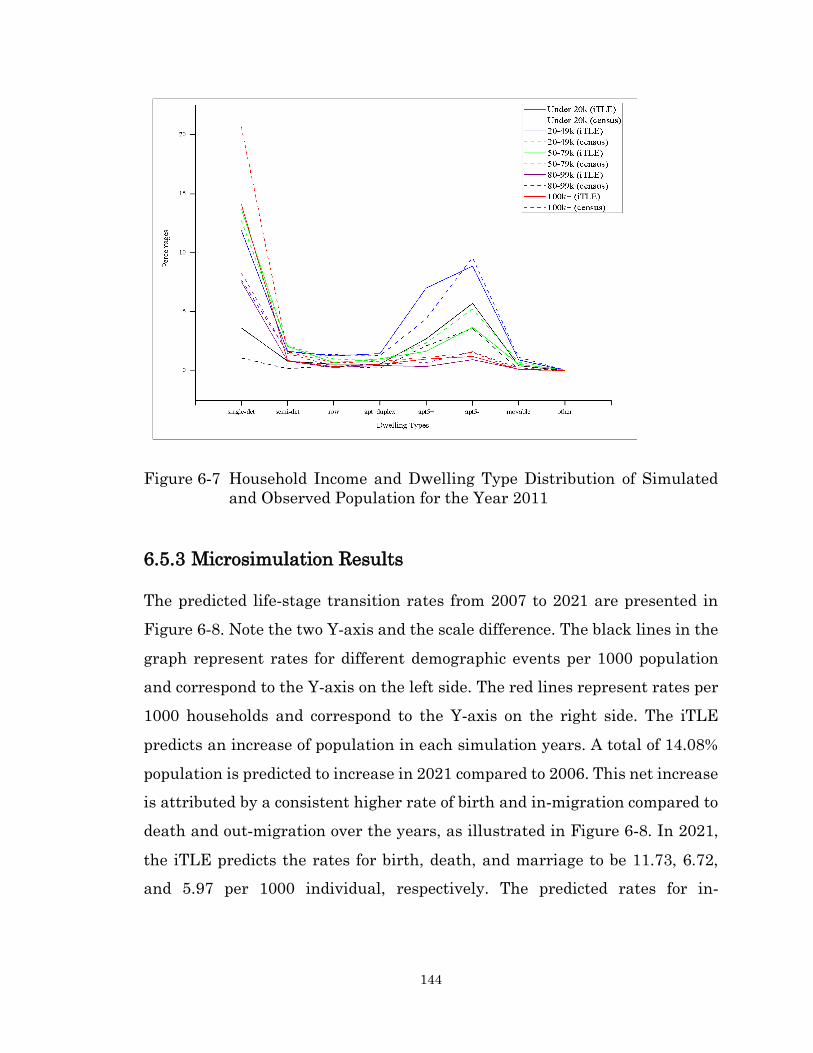
144
Figure 6-7 Household Income and Dwelling Type Distribution of Simulated
and Observed Population for the Year 2011
6.5.3 Microsimulation Results
The predicted life-stage transition rates from 2007 to 2021 are presented in
Figure 6-8. Note the two Y-axis and the scale difference. The black lines in the
graph represent rates for different demographic events per 1000 population
and correspond to the Y-axis on the left side. The red lines represent rates per
1000 households and correspond to the Y-axis on the right side. The iTLE
predicts an increase of population in each simulation years. A total of 14.08%
population is predicted to increase in 2021 compared to 2006. This net increase
is attributed by a consistent higher rate of birth and in-migration compared to
death and out-migration over the years, as illustrated in Figure 6-8. In 2021,
the iTLE predicts the rates for birth, death, and marriage to be 11.73, 6.72,
and 5.97 per 1000 individual, respectively. The predicted rates for in-
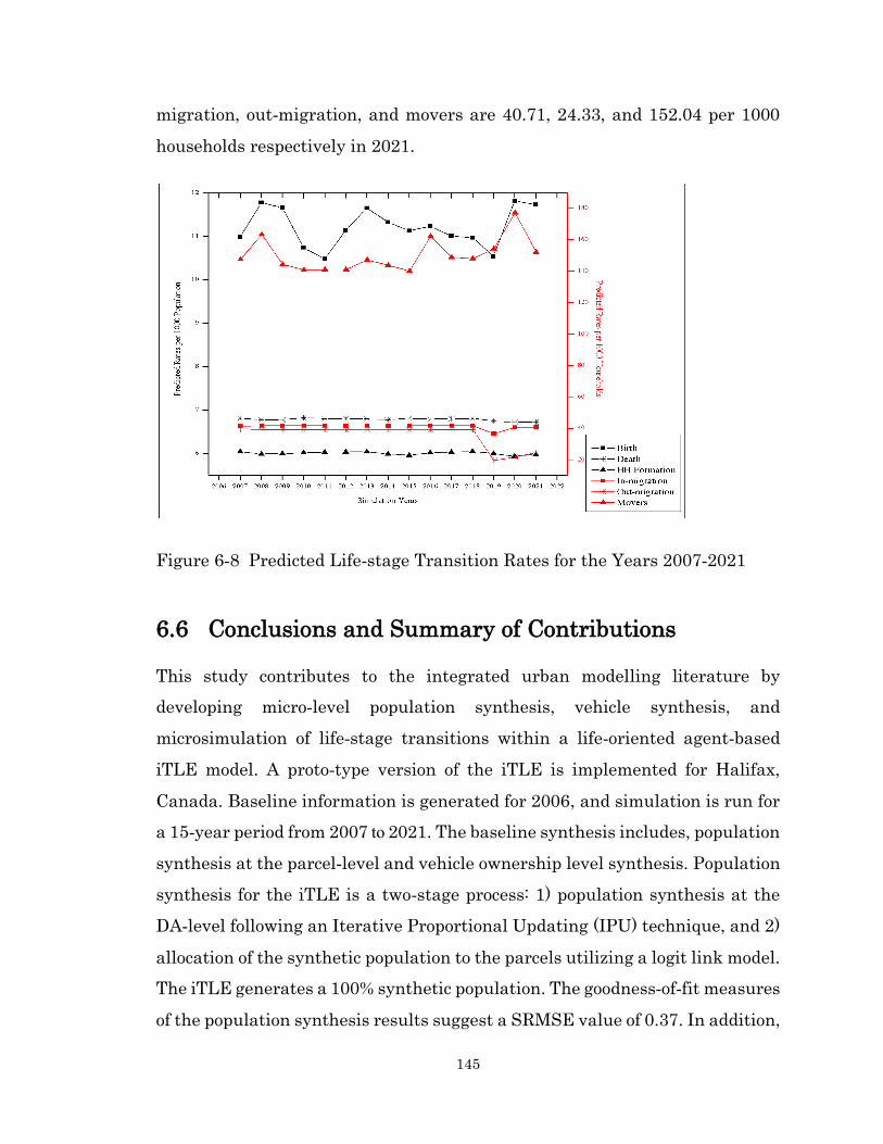
145
migration, out-migration, and movers are 40.71, 24.33, and 152.04 per 1000
households respectively in 2021.
Figure 6-8 Predicted Life-stage Transition Rates for the Years 2007-2021
6.6 Conclusions and Summary of Contributions
This study contributes to the integrated urban modelling literature by
developing micro-level population synthesis, vehicle synthesis, and
microsimulation of life-stage transitions within a life-oriented agent-based
iTLE model. A proto-type version of the iTLE is implemented for Halifax,
Canada. Baseline information is generated for 2006, and simulation is run for
a 15-year period from 2007 to 2021. The baseline synthesis includes, population
synthesis at the parcel-level and vehicle ownership level synthesis. Population
synthesis for the iTLE is a two-stage process: 1) population synthesis at the
DA-level following an Iterative Proportional Updating (IPU) technique, and 2)
allocation of the synthetic population to the parcels utilizing a logit link model.
The iTLE generates a 100% synthetic population. The goodness-of-fit measures
of the population synthesis results suggest a SRMSE value of 0.37. In addition,
146
around 89% of the DAs are found to show an APE measure of less than 5%. In
the case of vehicle ownership level synthesis, a MNL model is developed to
generate vehicle ownership in the following four levels: zero, one, two, and
three or more vehicle. The synthesis results suggest that 22.55%, 37.40%,
32.16%, and 7.859% of the households own zero, one, two, and three or more
vehicles, respectively.
The population life-stage transition module simulates a number of life-stages,
such as ageing, birth, death, in-migration, out-migration, and household
formation. Population life-stages are simulated following a heuristic modelling
approaches. In this process, historical rates and rules are developed to
determine the occurrence of an event for an individual/household in a
particular simulation year. The life-stage transition module is validated with
the Census 2011 information. A cross comparative analysis of the simulated
and observed population attributes is performed. The cross comparative
validation results suggest that majority of the categories of the population
socio-demographic attributes show a difference of less than 1%. In the case of
forecasting, the iTLE predicts an increase of 14.08% population in 2021
compared to 2006. The results suggest that the iTLE generates reasonably
satisfactory population estimates for further model development and
implementation.
In summary, the baseline synthesis and life-stage transition module developed
in this study resolve some key issues in integrated urban modelling, which will
assist in implementing state-of-the-art residential location and vehicle
transaction decision components within the iTLE framework. For example, the
life-stage transition component will assist in maintaining the multi-domain
decision interactions along the life-course of the agents. In addition, population
synthesis at the micro-spatial level enables iTLE to simulate agents decisions
and changes at the disaggregate spatial-level. Finally, the vehicle ownership
147
synthesis adds the capacity to the iTLE to perform vehicle ownership
simulation.

148
Chapter 7
7 Microsimulation of Residential
Location Processes
7.1 Introduction
This chapter presents the microsimulation of residential location transition
module of the iTLE model. The residential location module is implemented by
utilizing the micro-behavioural models developed in Chapter 4. This research
contributes to the mircosimulation paradigm of residential location in the
following three dimensions: 1) addressing the multi-domain interactions and
life-course dynamics during the simulation procedure, 2) accommodating the
process orientation of the phenomenon by implementing location decision as a
two-stage process of mobility and location choice, and 3) predicting the spatio-
temporal evolution of the population and demographic configuration of the
neighbourhoods. This study also offers a validation of the residential location
simulation results.
The organization of this chapter is as follows: section 7.2 discusses the
microsimulation processes of the mobility and location choice components of
the location transition module. Section 7.3 provides the validation results of
the module. Section 7.4 presents the microsimulation results, particularly,
prediction of the evolution of urban population. Finally, section 7.5 concludes
with a summary and potential use of the model.
The following paper is an earlier version of this chapter:
Fatmi, M.R., and Habib, M.A. (2017). Development of a Proto-type Integrated Urban
Model: Microsimulation of Life-stage Transitions and Residential Location
Transitions. Published in the peer-reviewed proceedings of the 96th Annual Meeting of
Transportation Research Board, Washington DC, USA, January 8-12.
149
7.2 Microsimulation Processes
The residential location transition module determines the choice of location as
a process of mobility and location choice. To reduce the computational
complexity, more compatible and simplified versions of the micro-behavioural
models developed in Chapter 4 are considered for the implementation within
the iTLE proto-type model system (Appendix B). The models maintain the
basic principle of the life-course perspective through accommodating the
effects of life-cycle events as lead and lag events. A description of the
microsimulation processes is provided below.
7.2.1 Residential Mobility
The household-level residential mobility decision is simulated in each year by
implementing a discrete time binomial logit model (Appendix B). The purpose
for developing this discrete time binomial logit model is that it is more
compatible for implementing within the discrete time simulation framework of
the iTLE than the continuous time duration model developed in Chapter 4. The
mobility model determines the probability of move of a household at a
particular simulation year. The predictors’ equation for the mobility model is
written below:
𝑌𝑖 = 𝑐 + 𝛼𝑋𝑖 + 휀 (1)
Here, 𝑖 is household, 𝑋 is the predictor, 𝑐 is the constant term, 휀 is the random
error term, and 𝛼 is the coefficient of the parameter to be estimated. Now the
probability equation can be written as:
𝑃(𝑌𝑖) =𝑒𝑐+𝛼𝑋𝑖
1+𝑒𝑐+𝛼𝑋𝑖 (2)
Households are assigned to move or stay list by comparing the estimated
probability of the move against a randomly generated probability using Monte
150
Carlo Simulation technique. If the estimated probability is higher than the
random probability, then households are assigned to move list and enter the
location choice process. In contrary, households are assigned to stay list and
exit the location transition module.
7.2.2 Residential Location Choice
The location choice of the households is simulated by using a multinomial logit
(MNL) model (Appendix B), which is a simplified version of the model
developed in Chapter 4. The spatial unit of simulation is at the parcel-level.
The utility function for the location choice model can be written as:
𝑉𝑖𝑗 = 𝛼𝑗𝑋𝑗 + 𝛼𝑗𝑖𝑋𝑗𝑋𝑖 + 휀 (3)
Here, 𝑖 is household, 𝑗 is parcel, 𝑋 is the predictor, 𝜖 is the random error term,
and 𝛼 is the coefficient of the parameter to be estimated. The term 𝑋𝑗𝑋𝑖
represents interaction variables. The probability function can be written in the
following logit form:
𝑃𝑖𝑗 = 𝛼𝑗𝑋𝑗+𝛼𝑗𝑖𝑋𝑗𝑋𝑖
∑ 𝛼𝑗𝑋𝑗+𝛼𝑗𝑖𝑋𝑗𝑋𝑖𝑗 (4)
This location choice model determines the probability of choosing a location
from a pool of randomly generated alternative locations. Based on the
probability estimation, households are either assigned to move to the new
location or stay at their current location. The allocation of a parcel to a
household is sequential and follows the order of probability estimation. If a
parcel is allocated to a household, it is made unavailable for other households.
Based on the choice of new location, household, individual, and parcel lists are
updated accordingly. The current version of the model only estimates location
choice of the home owners’. Renters’ location are simulated using a simplified
heuristic process.
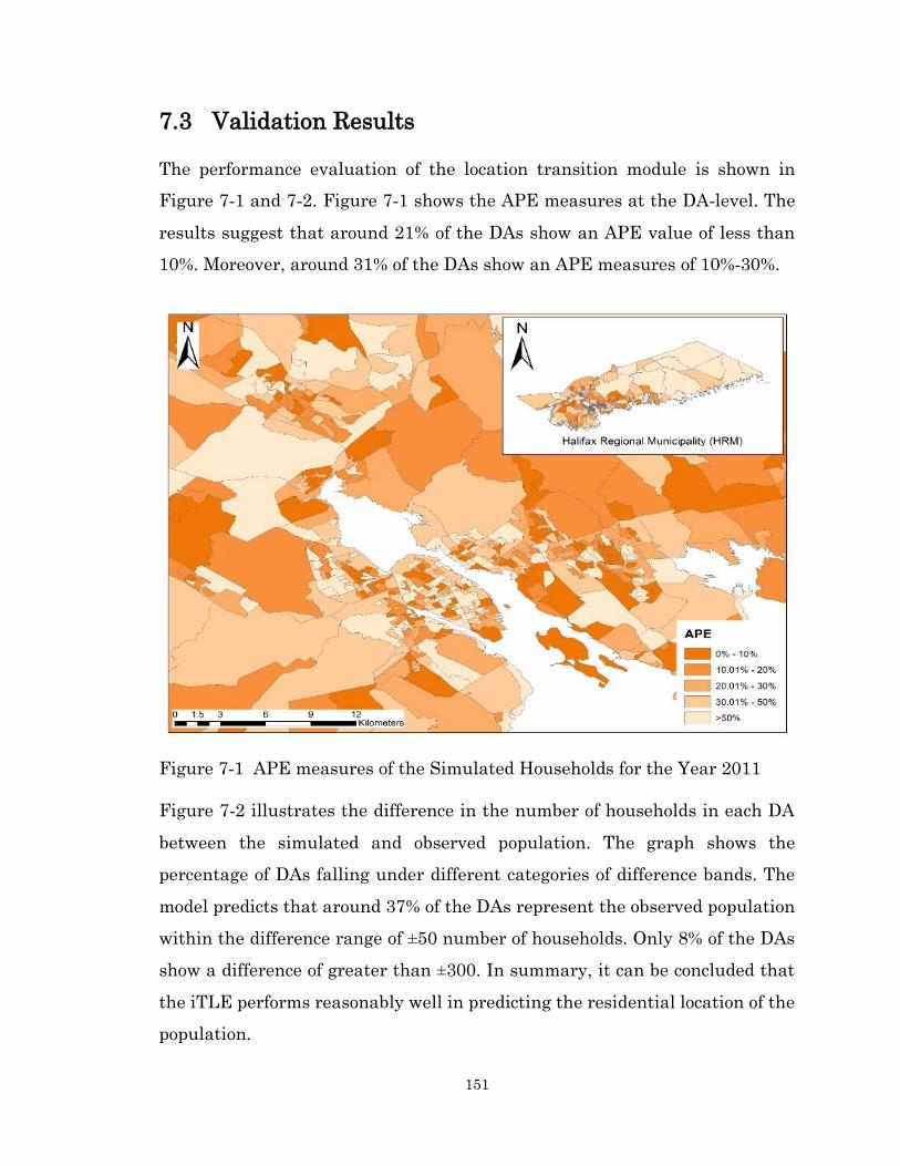
151
7.3 Validation Results
The performance evaluation of the location transition module is shown in
Figure 7-1 and 7-2. Figure 7-1 shows the APE measures at the DA-level. The
results suggest that around 21% of the DAs show an APE value of less than
10%. Moreover, around 31% of the DAs show an APE measures of 10%-30%.
Figure 7-1 APE measures of the Simulated Households for the Year 2011
Figure 7-2 illustrates the difference in the number of households in each DA
between the simulated and observed population. The graph shows the
percentage of DAs falling under different categories of difference bands. The
model predicts that around 37% of the DAs represent the observed population
within the difference range of ±50 number of households. Only 8% of the DAs
show a difference of greater than ±300. In summary, it can be concluded that
the iTLE performs reasonably well in predicting the residential location of the
population.
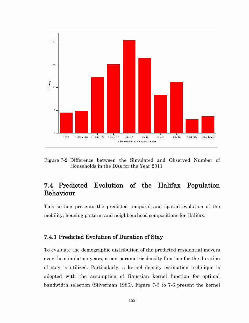
152
Figure 7-2 Difference between the Simulated and Observed Number of
Households in the DAs for the Year 2011
7.4 Predicted Evolution of the Halifax Population
Behaviour
This section presents the predicted temporal and spatial evolution of the
mobility, housing pattern, and neighbourhood compositions for Halifax.
7.4.1 Predicted Evolution of Duration of Stay
To evaluate the demographic distribution of the predicted residential movers
over the simulation years, a non-parametric density function for the duration
of stay is utilized. Particularly, a kernel density estimation technique is
adopted with the assumption of Gaussian kernel function for optimal
bandwidth selection (Silverman 1986). Figure 7-3 to 7-6 present the kernel

153
density plots of the predicted duration of stay for different age groups. Here,
age represents the age of the head of the household. The results suggest that
the density is skewed to the left for households with younger head. The density
is skewed to the right and is more variable as age increases. This implies that
younger head households are predicted to be more frequent movers than their
older counterpart. The mean of the duration for population with age <40, 40-
54, 55-64, and 65 and above are predicted to be 3.53, 6.05, 6.60, and 7.24 years
respectively.
Figure 7-3 Predicted Duration of Stay of Population Aged < 40 Years for the
Years 2007-2021

154
Figure 7-4 Predicted Duration of Stay of Population Aged 40-54 Years for the
Years 2007-2021
Figure 7-5 Predicted Duration of Stay of Population Aged 55-64 Years for the
Years 2007-2021

155
Figure 7-6 Predicted Duration of Stay of Population Aged > 64 Years for the
Years 2007-2021
To evaluate the predicted spatial evolution of duration of stay by
demographics, duration plot by location distance from CBD and age is
demonstrated in Figure 7-7. Location distance from CBD refers to the distance
of home parcel to the CBD, and age refers to the age of the head of the
household. Duration is predicted to increase as age and location distance from
CBD increases. This implies that younger head households residing closer to
the CBD are predicted to be more frequent movers than older head households
residing farther away from the CBD. As illustrated, duration is predicted to be
substantially high to the right of 45 years and above 10 km from the CBD,
revealing middle aged to older population residing in the suburban and rural
neighbourhoods are predicted to be less frequent movers. Similarly, the plot of
duration by location distance from CBD and household income in Figure 7-8
suggests that duration increases with household income and distance from
CBD. This implies that low income households residing closer to the CBD are
more frequent movers than their high income suburban and rural counterpart.
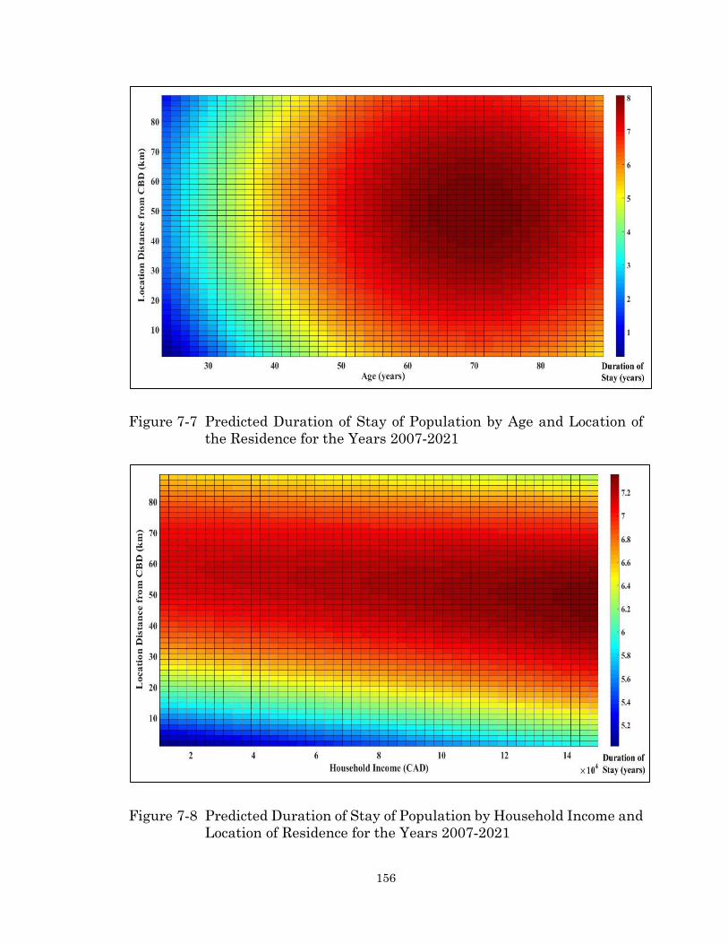
156
Figure 7-7 Predicted Duration of Stay of Population by Age and Location of
the Residence for the Years 2007-2021
Figure 7-8 Predicted Duration of Stay of Population by Household Income and
Location of Residence for the Years 2007-2021

157
7.4.2 Predicted Evolution of the Spatial Distribution of the
Halifax Population
Figure 7-9 illustrates population density change at the DA-level from 2006 to
2021. A higher increase in density is predicted in the high density urban core
(i.e. Halifax and Dartmouth urban core) and close by suburban areas (i.e.
Clayton Park, Bedford, and Sackville). Interestingly, a higher density increase
is predicted in the North End neighbourhoods of the Halifax Peninsula, which
is documented by Roth, (2013) as neighbourhoods experiencing gentrification.
Figure 7-9 Predicted Household Density Change from 2006 to 2021
The spatial distribution of the Halifax population in 2021 is presented in
Figure 7-10. The plot depicts the density of the households based on the
location (parcel) distance from the CBD. A higher proportion of the households

158
is predicted in the locations within 25km from the CBD. Similar findings can
be observed for the years 2007-2020, as reported in Appendix C. In the context
of Halifax, these are the high density urban core and nearby suburban
neighbourhoods, which corresponds to the high density areas in Figure 7-9.
The proportion of the population residing in these high density neighbourhoods
has increased over the 15 year periods. For example, 68% of the total
households were predicted in these high density areas in 2007, which increased
to 71% in 2021. The predicted evolution of the demographic composition of the
high density neighbourhoods is discussed in the next section.
Figure 7-10 Predicted Spatial Distribution of the Halifax Population for the
Year 2021

159
7.4.3 Predicted Demographic Composition of the High Density
Neighbourhoods in Halifax
The predicted average density of the high density12 neighbourhoods over the
simulation years is presented in Figure 7-11. The plot shows the yearly average
of the household density in each DA that falls under the high density category.
As illustrated, average household density is predicted to increase in the high
density DAs; to be specific, an average increase by around 632 household/sqkm
in 2021 compared to 2007.
Figure 7-11 Predicted Yearly Avg. Household Density of the High Density
DAs in Halifax for the Years 2007-2021
The distribution of the predicted average household income and average age
in the high density DAs from 2007-2021 is shown in Figure 7-12 to 7-15. The
12 High density neighbourhoods refer to the DAs with greater than 600 households per square
km.
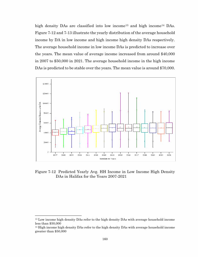
160
high density DAs are classified into low income13 and high income14 DAs.
Figure 7-12 and 7-13 illustrate the yearly distribution of the average household
income by DA in low income and high income high density DAs respectively.
The average household income in low income DAs is predicted to increase over
the years. The mean value of average income increased from around $40,000
in 2007 to $50,000 in 2021. The average household income in the high income
DAs is predicted to be stable over the years. The mean value is around $70,000.
Figure 7-12 Predicted Yearly Avg. HH Income in Low Income High Density
DAs in Halifax for the Years 2007-2021
13 Low income high density DAs refer to the high density DAs with average household income
less than $50,000 14 High income high density DAs refer to the high density DAs with average household income
greater than $50,000

161
Figure 7-13 Predicted Yearly Avg. HH Income in High Income High Density
DAs in Halifax for the Years 2007-2021
Figure 7-14 and 7-15 portray the yearly distribution of the average age by DA
in low income and high income high density DAs respectively. Note that age
refers to the age of the head of the household. Average age of the head of the
household is predicted to increase in both the low and high income DAs. In the
case of the low income DAs, the mean value of average age increased from
around 50 years in 2007 to 58 years in 2021. For high income DAs, the mean
value increased from around 52 years in 2007 to 61 years in 2021.
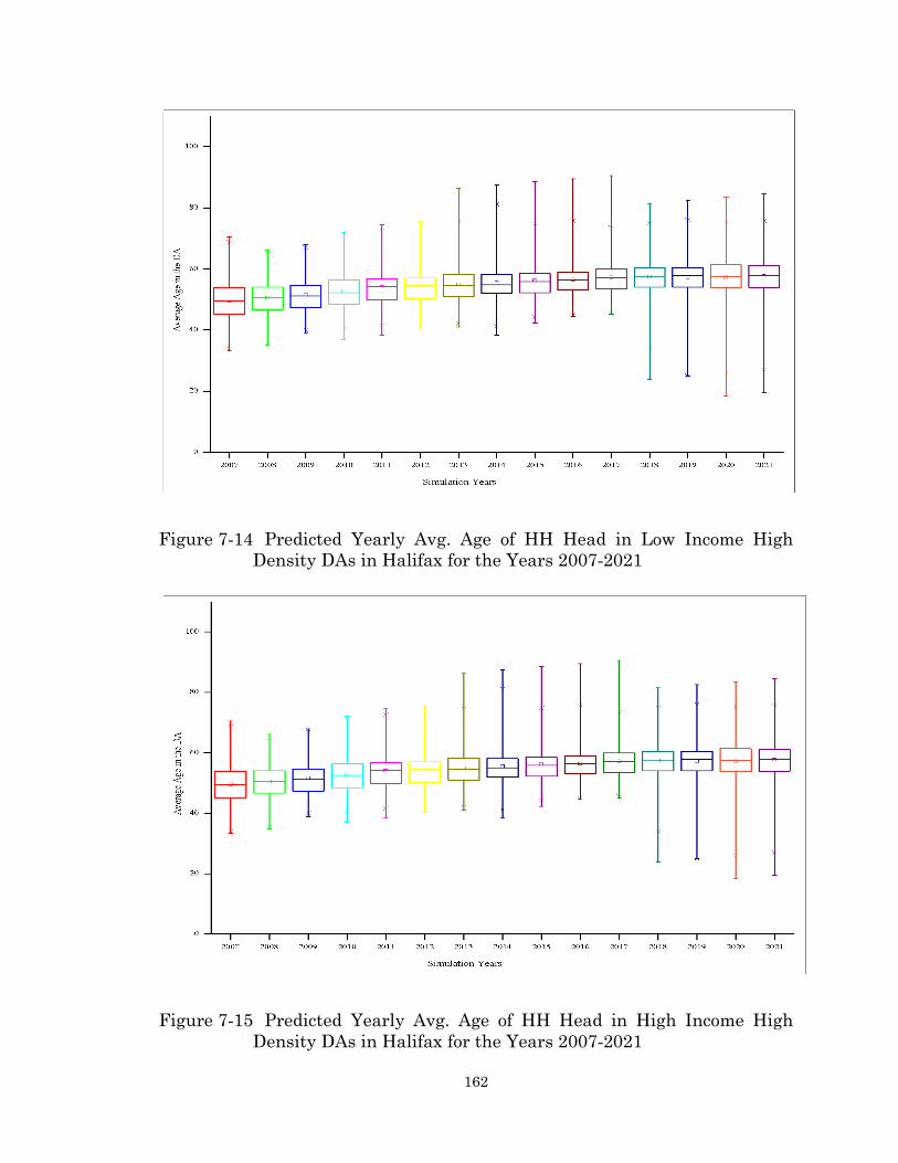
162
Figure 7-14 Predicted Yearly Avg. Age of HH Head in Low Income High
Density DAs in Halifax for the Years 2007-2021
Figure 7-15 Predicted Yearly Avg. Age of HH Head in High Income High
Density DAs in Halifax for the Years 2007-2021
163
The configuration of the high density neighbourhoods in terms of its
population’s demographics and household composition in 2021 is illustrated in
Figure 7-16 to 7-20. Kernel density is plotted against the home location (parcel)
distance from CBD for population with different household composition. In
each figure from 7-16 to 7-20, three kernel density are estimated for low
income15, medium income16, and high income17 households. The kernel density
estimation assumes a Gaussian kernel function for optimal bandwidth
selection. Fig 7-16 depicts that the density is skewed towards the left of 5km
for single person households. Interestingly, the density is predicted to be more
variable and skewed towards the right of 5km as household composition
changes through life-events (i.e. marriage, having children), as shown in Fig 7-
17 to 7-20. For example, a secondary peak in the density is predicted for couple
without children for locations within 10-15km. Locations within 10-15km from
the CBD in Halifax refer to suburban neighbourhoods. This implies that as
household composition changes through marriage and birth of a child,
households’ density is skewed towards the suburban neighbourhoods. In the
case of variation by household income, the density of high income households
is skewed to the left of 5km and within 10-15km. For low and medium income
households, density is skewed to the left of 10km. Interestingly, for couple with
more than two children, the variation by income is predicted to be relatively
small. Similar observations can be made for other simulation years as well.
15 Low income refers to household income less than $50,000 16 Medium income refers to household income between $50,000 and $100,000 17 High income refers to household income above $100,000

164
Figure 7-16 Predicted Distribution of Single Person HH in the High Density
Neighbourhoods of Halifax for the Year 2021
Figure 7-17 Predicted Distribution of Couple without Child HH in the High
Density Neighbourhoods of Halifax for the Year 2021
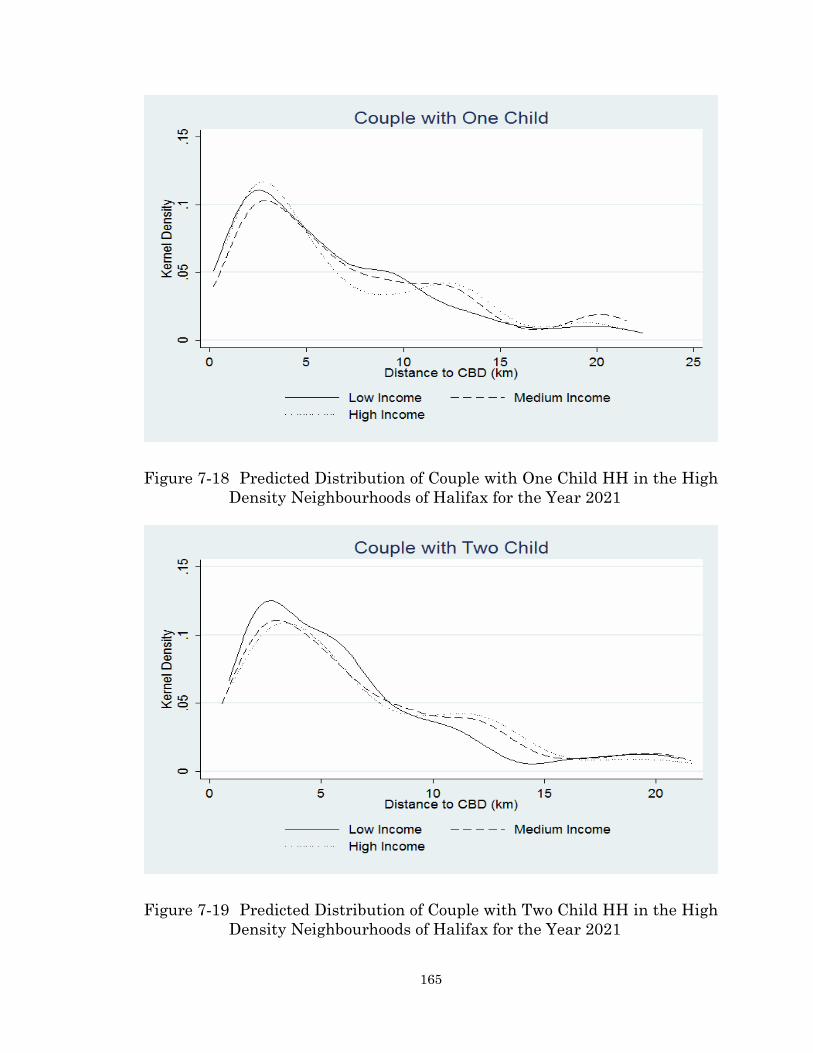
165
Figure 7-18 Predicted Distribution of Couple with One Child HH in the High
Density Neighbourhoods of Halifax for the Year 2021
Figure 7-19 Predicted Distribution of Couple with Two Child HH in the High
Density Neighbourhoods of Halifax for the Year 2021
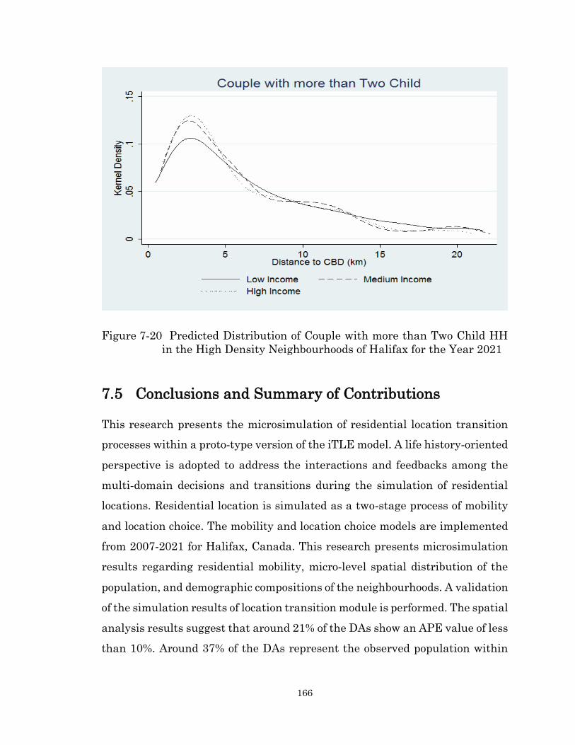
166
Figure 7-20 Predicted Distribution of Couple with more than Two Child HH
in the High Density Neighbourhoods of Halifax for the Year 2021
7.5 Conclusions and Summary of Contributions
This research presents the microsimulation of residential location transition
processes within a proto-type version of the iTLE model. A life history-oriented
perspective is adopted to address the interactions and feedbacks among the
multi-domain decisions and transitions during the simulation of residential
locations. Residential location is simulated as a two-stage process of mobility
and location choice. The mobility and location choice models are implemented
from 2007-2021 for Halifax, Canada. This research presents microsimulation
results regarding residential mobility, micro-level spatial distribution of the
population, and demographic compositions of the neighbourhoods. A validation
of the simulation results of location transition module is performed. The spatial
analysis results suggest that around 21% of the DAs show an APE value of less
than 10%. Around 37% of the DAs represent the observed population within
167
the difference range ±50 number of households. Hence, the simulation results
are considered as satisfactory.
Further microsimulation results provide interesting insights towards the
micro-level spatio-temporal evolution of population mobility, housing pattern,
and household compositions of the neighbourhoods. The mobility results
suggest that younger head households are more frequent movers than their
older counterpart. The mean duration of stay of the population with age <40,
40-54, 55-64, and 65 and above are predicted to be 3.53, 6.05, 6.60, and 7.24
years, respectively. Particularly, younger head households residing closer to
the CBD are predicted to be more frequent movers than older head households
residing farther away from the CBD. The spatial distribution suggests that a
higher density of the households is consistently predicted in the locations
within 25km from the CBD over the simulation years of 2007-2021. The
proportion of total households is predicted to increase from 68% in 2007 to 71%
in 2021 in these high density neighbourhoods. In terms of the DA-level
demographics and household compositional configuration of the high density
neighbourhoods, higher density of single person households are predicted in
the urban core. As household composition changes through marriage and
having child, the density is predicted to be more variable and skewed towards
the suburban neighbourhoods.
The capacity of iTLE to generate micro-level spatial distribution of the
population will be useful for testing alternative land use and transport policies.
It will also feed important information to develop state-of-the-art activity-
based travel models. For instance, the micro-level prediction of the spatio-
temporal evolution of population demographics will be useful for destination
choice procedure. It will assist in addressing the variation in activity
generation and scheduling procedure for population at different life-stages
residing in different locations. Moreover, the iTLE will support substantial

168
intra-household interactions during the simulation of travel activities, such as
scheduling, vehicle allocation, and mode choice.
169
Chapter 8
8 Microsimulation of Vehicle
Transactions
8.1 Introduction
This chapter presents the microsimulation of vehicle transaction component of
the iTLE model. The contributions of this research is three-fold: 1)
microsimulating vehicle transaction decisions, 2) addressing the process
orientation of the phenomenon through simulating first time purchase,
transaction or do nothing, acquisition, trade, and disposal decisions, and 3)
accommodating the multi-way interaction of various life-cycle events and
decisions during the simulation procedure. This research presents the
validation results and offers insights towards how vehicle transaction as well
as ownership is spatio-temporally evolving by population demographics.
This chapter is organized as follows: section 8.2 discusses the microsimulation
processes of the vehicle transaction component within the iTLE. Section 8.3
describes the simulation results including validation and predicted evolution
of vehicle ownership for the Halifax population. Finally, section 8.4 concludes
with a summary of key findings.
The following paper is an earlier version of this chapter:
Fatmi, M.R., and Habib, M.A. (2017). Microsimulation of Vehicle Transaction
Decisions within an Integrated Urban Modeling Framework. Published in the peer-
reviewed proceedings of the 96th Annual Meeting of Transportation Research Board,
Washington DC, USA, January 8-12.
170
8.2 Microsimulation Processes
The operational framework of the vehicle transaction component within the
iTLE model is presented in Figure 8-1. The process starts with a vehicle
ownership synthesis component to generate baseline vehicle ownership
information. Description of this component is provided in Chapter 6. Following
the generation of baseline vehicle information, vehicle transaction component
operates as a sequential process of vehicle ownership state and transaction.
The first step in this process is to assign households into the following two
categories of vehicle ownership state: no vehicle ownership state, and transient
ownership state. The next step is to determine the following vehicle transaction
decisions: first time purchase, transaction or do nothing, acquisition, disposal,
and trade. Simplified version of the model developed in Chapter 5 are
implemented within the iTLE proto-type. Discussion on the microsimulation
processes and methods are provided below.
8.2.1 Vehicle Ownership State
In this stage, the vehicle ownership state of each household is determined in
each simulation year. Households are heuristically assigned into one of the
following two categories of vehicle ownership state: no vehicle ownership state,
and transient ownership state. Households without a vehicle transaction
history in their life-time are assigned to the list of no vehicle ownership state,
and households with a transaction history are assigned to the list of transient
ownership state.
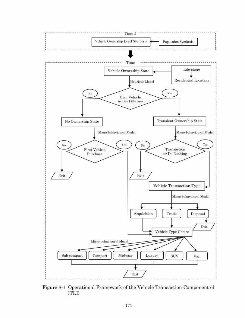
171
Vehicle Ownership State
Own Vehicle
in the Lifetime
No Ownership State
First Vehicle
Purchase
Transient Ownership State
Transaction
or Do Nothing
Acquisition Disposal Trade
Vehicle Type Choice
Vehicle Transaction Type
Sub-compact Compact Mid-size Luxury SUV Van
Exit Exit
Exit
No Yes
Exit
Heuristic Model
Micro-behavioural Model Micro-behavioural Model
Micro-behavioural Model
Micro-behavioural Model
Vehicle Ownership Level Synthesis
Time t
Population Synthesis
Life-stage
Residential Location
No Yes No Yes
Time
t+n
Figure 8-1 Operational Framework of the Vehicle Transaction Component of
iTLE
171
172
8.2.2 First Time Vehicle Purchase
In each simulation year, the first time vehicle purchase decision is simulated
for the households in the no vehicle ownership state list, since they never
owned a vehicle in their life-time. For the first vehicle purchase, a discrete time
binomial logit model is developed utilizing the HMTS data (Appendix B).
Households are identified to purchase the first vehicle or not by comparing the
estimated probability with a randomly generated probability using Monte
Carlo Simulation technique. If the estimated probability is higher, households
are assigned to the list of first vehicle purchase and enter vehicle type choice
component. Otherwise, households exit the vehicle ownership transition
module.
8.2.3 Vehicle Transaction or Do Nothing
In the case of the households in the list of transient ownership state, their
transaction or do nothing decisions are simulated. A discrete time binomial
logit modelling technique (similar method to the first vehicle purchase model)
is utilized to determine the probability of a household to make a transaction
(Appendix B). The estimated probability is compared with a random
probability to identify whether households make a transaction or not in a year.
Households assigned to the list of transaction, enter vehicle transaction type
component. Households assigned to the list of no transaction, exit the module.
8.2.4 Vehicle Transaction Type
Vehicle transaction type component involves the simulation of acquisition,
disposal, and trade. Transaction type model is developed utilizing a
multinomial logit modelling technique (Appendix B). The model determines
the probability of a household to make one of the three transactions following
173
the order of probability estimation. Households assigned to acquire or trade
enter vehicle type choice component. Households assigned to make a disposal
exit the module. Subsequently, the vehicle ownership level of the households
making a transaction is updated accordingly.
The next step is to simulate vehicle type choice. In this stage, the simulation
determines the choice among the following six vehicle types: sub-compact,
compact, mid-size, luxury, SUV, and van. The micro-behavioural model of the
vehicle type choice component is recently developed (Khan and Habib 2016),
and will be implemented later.
8.3 Validation Results
The iTLE proto-type runs vehicle transaction simulation from 2007 to 2021.
The simulation results of the vehicle transaction component are validated for
the 2016 simulation year using the NovaTRAC18 2016 survey data. A
comparison of the vehicle ownership level between the predicted and observed
population is presented in Figure 8-2. The comparative analysis suggests that
the iTLE under-represents zero vehicle ownership by 1%. Two, and three or
more vehicle ownerships are over-represented by 2%, and 3% respectively. The
largest difference is found for one vehicle ownership, which is an under-
representation of 4%, only. Therefore, the validation results reveal that the
performance of the vehicle transaction component can be considered
reasonably satisfactory.
18 NovaTRAC is a travel activity survey conducted in the Province of Nova Scotia. The survey
collected vehicle ownership information as well as travel activities of the population.
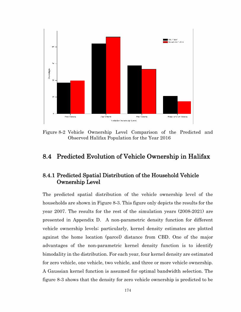
174
Figure 8-2 Vehicle Ownership Level Comparison of the Predicted and
Observed Halifax Population for the Year 2016
8.4 Predicted Evolution of Vehicle Ownership in Halifax
8.4.1 Predicted Spatial Distribution of the Household Vehicle
Ownership Level
The predicted spatial distribution of the vehicle ownership level of the
households are shown in Figure 8-3. This figure only depicts the results for the
year 2007. The results for the rest of the simulation years (2008-2021) are
presented in Appendix D. A non-parametric density function for different
vehicle ownership levels; particularly, kernel density estimates are plotted
against the home location (parcel) distance from CBD. One of the major
advantages of the non-parametric kernel density function is to identify
bimodality in the distribution. For each year, four kernel density are estimated
for zero vehicle, one vehicle, two vehicle, and three or more vehicle ownership.
A Gaussian kernel function is assumed for optimal bandwidth selection. The
figure 8-3 shows that the density for zero vehicle ownership is predicted to be

175
skewed to the left of 10km over the years, which are urban core neighbourhoods
in Halifax. The density is predicted to be more variable as households’ vehicle
ownership level goes higher. For example, two, and three or more vehicle
ownership are predicted to be more variable and skewed to the left of 25km. In
the context of Halifax, parcels within 25km of the CBD represent both urban
and suburban neighbourhoods. This implies that households with higher
vehicle ownership are not only distributed in the suburban neighbourhoods, a
reasonable share is distributed in the urban core as well. Interestingly, the
density of households with three or more vehicle ownership is predicted to
increase to the left of 10km over the years. This increase of three or more
vehicle ownership in the Halifax urban core over the years might be attributed
by the positive relationship of the variable “distance from home to CBD less
than 10km”, retained in the vehicle acquisition choice scenario of the
transaction type model (see Appendix B).
Figure 8-3 Predicted Distribution of Vehicle Ownership Level by Home
Location for the Year 2007
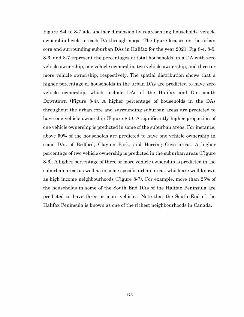
176
Figure 8-4 to 8-7 add another dimension by representing households’ vehicle
ownership levels in each DA through maps. The figure focuses on the urban
core and surrounding suburban DAs in Halifax for the year 2021. Fig 8-4, 8-5,
8-6, and 8-7 represent the percentages of total households’ in a DA with zero
vehicle ownership, one vehicle ownership, two vehicle ownership, and three or
more vehicle ownership, respectively. The spatial distribution shows that a
higher percentage of households in the urban DAs are predicted to have zero
vehicle ownership, which include DAs of the Halifax and Dartmouth
Downtown (Figure 8-4). A higher percentage of households in the DAs
throughout the urban core and surrounding suburban areas are predicted to
have one vehicle ownership (Figure 8-5). A significantly higher proportion of
one vehicle ownership is predicted in some of the suburban areas. For instance,
above 50% of the households are predicted to have one vehicle ownership in
some DAs of Bedford, Clayton Park, and Herring Cove areas. A higher
percentage of two vehicle ownership is predicted in the suburban areas (Figure
8-6). A higher percentage of three or more vehicle ownership is predicted in the
suburban areas as well as in some specific urban areas, which are well known
as high income neighbourhoods (Figure 8-7). For example, more than 25% of
the households in some of the South End DAs of the Halifax Peninsula are
predicted to have three or more vehicles. Note that the South End of the
Halifax Peninsula is known as one of the richest neighbourhoods in Canada.
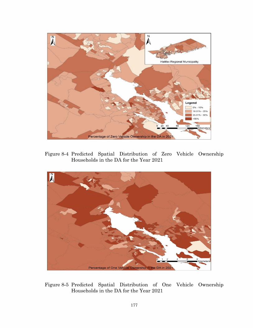
177
Figure 8-4 Predicted Spatial Distribution of Zero Vehicle Ownership
Households in the DA for the Year 2021
Figure 8-5 Predicted Spatial Distribution of One Vehicle Ownership
Households in the DA for the Year 2021

178
Figure 8-6 Predicted Spatial Distribution of Two Vehicle Ownership
Households in the DA for the Year 2021
Figure 8-7 Predicted Spatial Distribution of Three or More Vehicle Ownership
Households in the DA for the Year 2021

179
8.4.2 Predicted Vehicle Transactions by Population Demographics
A 2-dimensional kernel density is estimated to evaluate the predicted vehicle
transaction types by population demographics. Similar to the above kernel
estimates, a Gaussian kernel function for optimal bandwidth selection is
assumed. Figure 8-8 to 8-11 illustrate the 2-dimensional kernel estimates for
different transaction types for the year 2021. The kernel plots for the first
purchase, acquisition, disposal, and trade are shown in Figure 8-8, 8-9, 8-10,
and 8-11, respectively. In each figure, x-axis represents age of the head of the
household, y-axis represents household income, and z-axis is the color bar
representing kernel density. For the first vehicle purchase, density is skewed
to the left of 45 years and household income of less than $80,000 (Figure 8-8).
This implies that higher proportion of the first vehicle purchase is made by
younger head households with lower and middle income. The average age and
household income for first vehicle purchase is 39 years and $33,000
respectively, which further indicates a higher share of lower income younger
groups. In the case of vehicle acquisition, the density is predicted to be more
variable than first purchase. The density is skewed within the age range of 35-
65 years and income of less than $120,000 (Figure 8-9). This reflects that
population with a wider range of demographics are predicted to be involved in
vehicle acquisition. The average age and household income for acquisition is
49 years and $47,000 respectively. For disposal, density is skewed within 35-
65 years and $30,000-$110,000 (Figure 8-10). The average age is 53 years and
household income is $73,000. In the case of trade, density is skewed within 40-
80 years and within the income range of $130,000-$170,000 (Figure 8-11). This
implies that older head high income households are predicted to make a higher
proportion of vehicle trade. The average age is 60 years and household income
is $80,000 for the trade. The average income of $80,000 is lower than the
skewed range of $130,000-$170,000. This can be explained by the secondary
peaks in the kernel estimates for the same age range but lower income range.
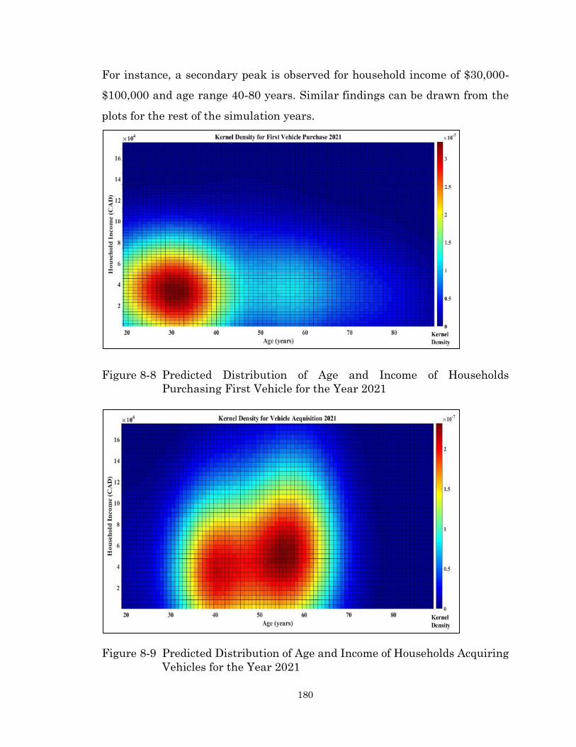
180
For instance, a secondary peak is observed for household income of $30,000-
$100,000 and age range 40-80 years. Similar findings can be drawn from the
plots for the rest of the simulation years.
Figure 8-8 Predicted Distribution of Age and Income of Households
Purchasing First Vehicle for the Year 2021
Figure 8-9 Predicted Distribution of Age and Income of Households Acquiring
Vehicles for the Year 2021
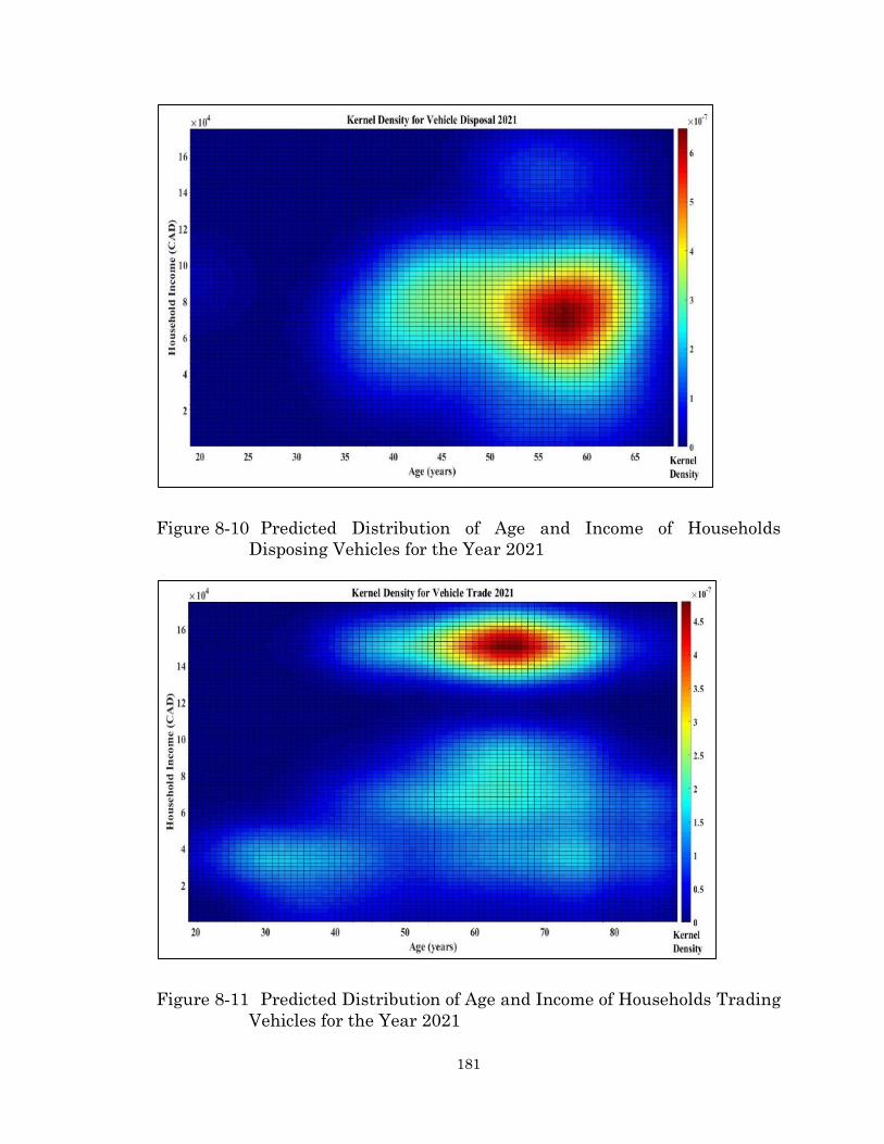
181
Figure 8-10 Predicted Distribution of Age and Income of Households
Disposing Vehicles for the Year 2021
Figure 8-11 Predicted Distribution of Age and Income of Households Trading
Vehicles for the Year 2021
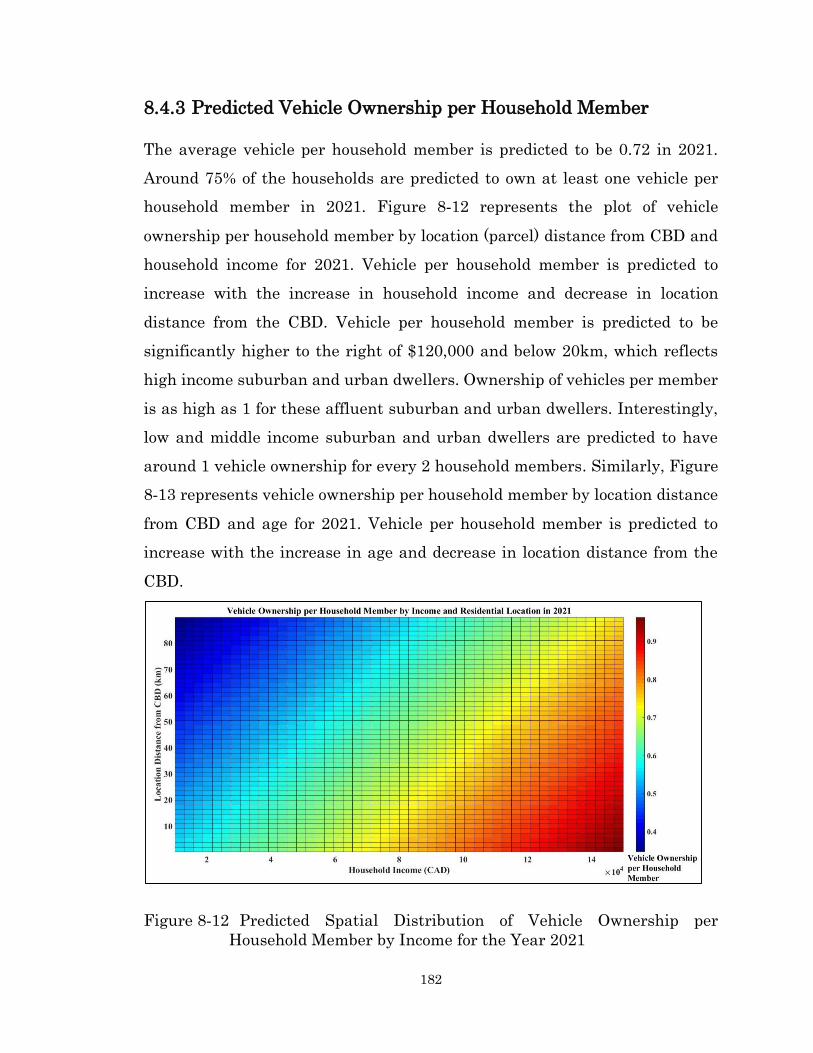
182
8.4.3 Predicted Vehicle Ownership per Household Member
The average vehicle per household member is predicted to be 0.72 in 2021.
Around 75% of the households are predicted to own at least one vehicle per
household member in 2021. Figure 8-12 represents the plot of vehicle
ownership per household member by location (parcel) distance from CBD and
household income for 2021. Vehicle per household member is predicted to
increase with the increase in household income and decrease in location
distance from the CBD. Vehicle per household member is predicted to be
significantly higher to the right of $120,000 and below 20km, which reflects
high income suburban and urban dwellers. Ownership of vehicles per member
is as high as 1 for these affluent suburban and urban dwellers. Interestingly,
low and middle income suburban and urban dwellers are predicted to have
around 1 vehicle ownership for every 2 household members. Similarly, Figure
8-13 represents vehicle ownership per household member by location distance
from CBD and age for 2021. Vehicle per household member is predicted to
increase with the increase in age and decrease in location distance from the
CBD.
Figure 8-12 Predicted Spatial Distribution of Vehicle Ownership per
Household Member by Income for the Year 2021
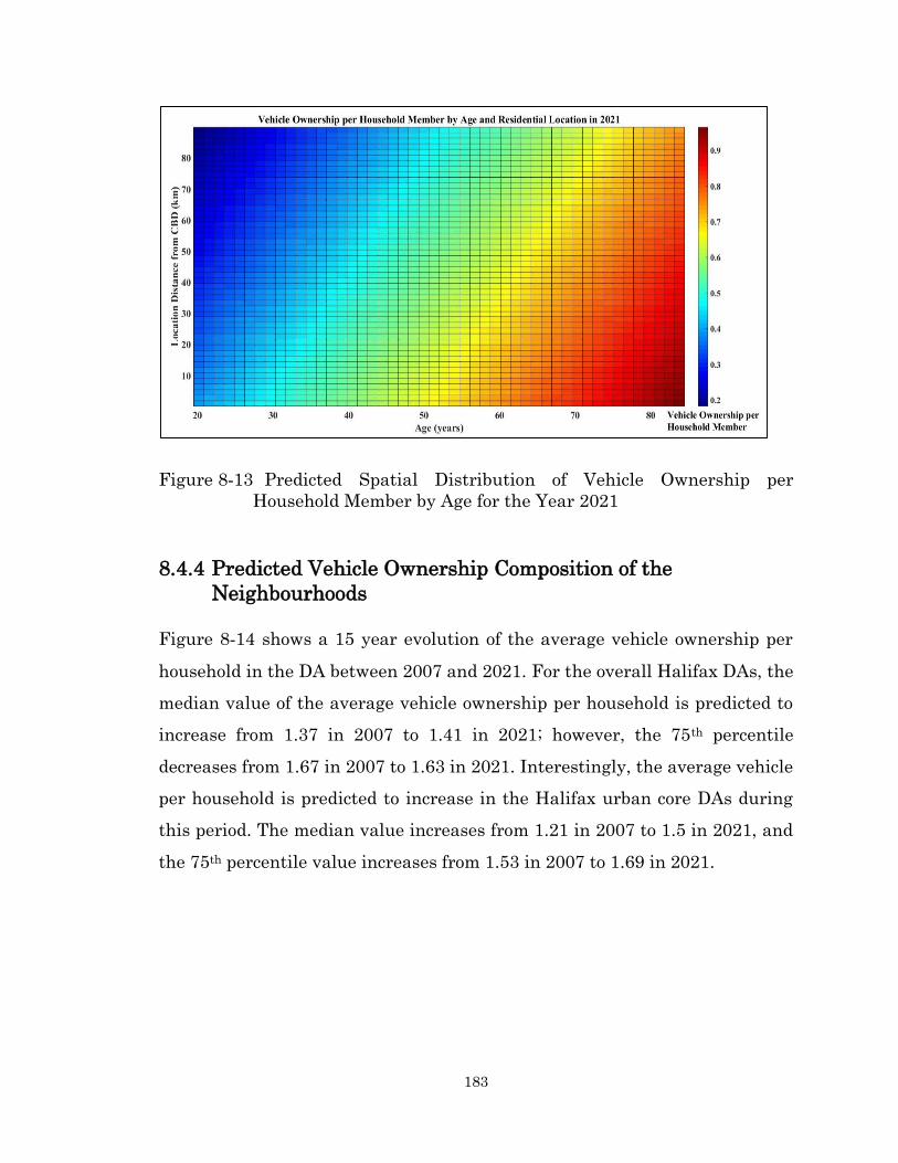
183
Figure 8-13 Predicted Spatial Distribution of Vehicle Ownership per
Household Member by Age for the Year 2021
8.4.4 Predicted Vehicle Ownership Composition of the
Neighbourhoods
Figure 8-14 shows a 15 year evolution of the average vehicle ownership per
household in the DA between 2007 and 2021. For the overall Halifax DAs, the
median value of the average vehicle ownership per household is predicted to
increase from 1.37 in 2007 to 1.41 in 2021; however, the 75th percentile
decreases from 1.67 in 2007 to 1.63 in 2021. Interestingly, the average vehicle
per household is predicted to increase in the Halifax urban core DAs during
this period. The median value increases from 1.21 in 2007 to 1.5 in 2021, and
the 75th percentile value increases from 1.53 in 2007 to 1.69 in 2021.
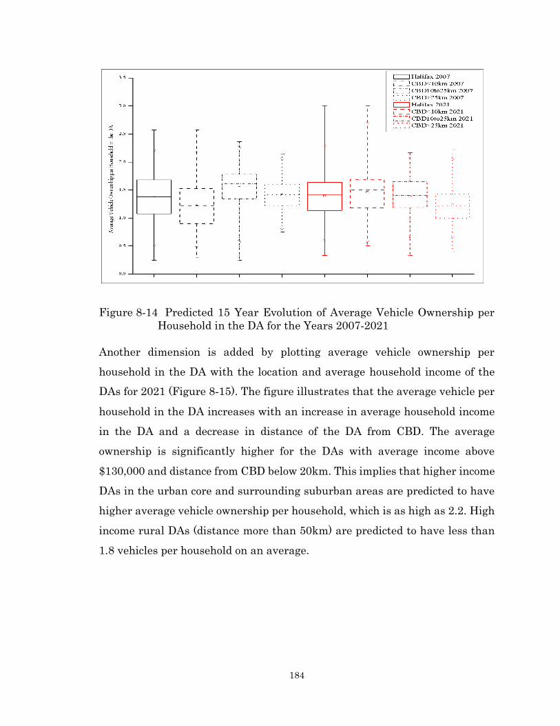
184
Figure 8-14 Predicted 15 Year Evolution of Average Vehicle Ownership per
Household in the DA for the Years 2007-2021
Another dimension is added by plotting average vehicle ownership per
household in the DA with the location and average household income of the
DAs for 2021 (Figure 8-15). The figure illustrates that the average vehicle per
household in the DA increases with an increase in average household income
in the DA and a decrease in distance of the DA from CBD. The average
ownership is significantly higher for the DAs with average income above
$130,000 and distance from CBD below 20km. This implies that higher income
DAs in the urban core and surrounding suburban areas are predicted to have
higher average vehicle ownership per household, which is as high as 2.2. High
income rural DAs (distance more than 50km) are predicted to have less than
1.8 vehicles per household on an average.

185
Figure 8-15 Predicted Spatial Distribution of the Avg. Vehicle Ownership per
Household in the DA by Avg. Household Income in the DA for the
Year 2021
8.5 Conclusion
This research presents the findings of the microsimulation of vehicle
transaction component within the iTLE proto-type model. The process
orientation of vehicle transaction is addressed by microsimulating first time
purchase, transaction or do nothing, acquisition, trade, and disposal decisions.
The effects of multi-domain decision interactions and life-stage transitions on
vehicle transaction decisions is accommodated within the simulation
framework.
The iTLE proto-type simulates vehicle transactions for 2007-2021 for Halifax.
The validation results at the 2016 time point suggests that majority of the
categories of the predicted vehicle ownership levels lie within a few percentage
186
point of the observed ownership level. For example, zero vehicle ownership is
under represented by 1%, only. Therefore, it can be concluded that the iTLE
generates reasonably representative vehicle ownership estimates for the
population.
This research also presents simulation results regarding the spatio-temporal
distribution of vehicle ownership for the Halifax population. A yearly spatial
variation of different vehicle ownership levels is presented by kernel density
estimates. It is found that higher proportion of the households with zero vehicle
ownership is predicted in the Halifax urban core. The density is predicted to
be more variable and distributed in the suburban areas as well as urban areas
with the increase in vehicle ownership level. One of the interesting findings is
that an increase in density of three or more vehicle ownership households is
predicted in the urban core areas over the years. Similar distribution is found
while the percentage of different vehicle ownership level in the DAs is
represented through maps for the year 2021. The map shows that a higher
percentage of three or more vehicle ownership is predicted in some specific
urban areas, which are well known as high income neighbourhoods. The
demographic distribution of the vehicle transaction types suggests that higher
proportion of the first vehicle purchase involves younger head (average age 39
years) lower income (average household income $33,000) households. The
distribution of acquisition suggests that population with a wider range of
demographics are involved in acquisition, such as age range of 35-65 years and
income of less than $120,000. The average vehicle per household member is
predicted to be 0.72 in 2021 and around 75% of the households are predicted
to own at least one vehicle per household member in 2021. High income urban
dwellers are predicted to have a higher number of vehicles per member, which
is as high as 1 in 2021. The vehicle ownership level composition analysis of the
neighbourhoods (DA-level) suggests that the higher income DAs in the urban
187
core and surrounding suburban areas are predicted to have higher average
vehicle ownership per household, which is as high as 2.2 in 2021.
In summary, this study contributes significantly to the literature by
simulating vehicle transaction decisions as a process of first time purchase,
acquisition, disposal, trade, and transaction or do nothing decisions, within an
integrated urban modelling platform. Multi-way decision dynamics are
accommodated within the simulation procedure. The simulation results of
vehicle transaction decisions are reasonably satisfactory and offers promising
insights towards the spatio-temporal evolution of vehicle ownership in an
urban region. Future research should focus on the implementation of vehicle
type choice model. Finally, the implementation of vehicle transaction decisions
promises to improve the prediction of travel activities and facilitates the
opportunity to extend iTLE into the prediction of emission and energy use
under different policy scenarios.
188
Chapter 9
9 Conclusions
9.1 Summary
The development of integrated urban models have emerged from the need to
predict the evolution of urban region, and test alternative land use and
transport policy scenarios. Integrated urban models simulate a wide range of
household- and individual-level decision processes. Residential location and
vehicle ownership are two most critical components of integrated urban
models, since these are crucial household-level long-term and medium-term
decisions. One of the major limitations of the existing urban models is their
lack of behavioural representation during the modelling and simulation of
essential decision components. Unless the behaviour of the
individuals/households are reasonably addressed, the purpose for developing
integrated urban models will be challenging to achieve. This research
contributes to the modelling and microsimulation paradigms of integrated
urban models by representing greater behaviour of the population.
Particularly, this study presents the development and implementation of the
residential location and vehicle transaction components within an integrated
Transport Land Use and Energy (iTLE) modelling system. This study also
presents the implementation of population synthesis, vehicle ownership level
synthesis, and life-stage transition components within the iTLE model.
The research gaps in integrated urban modelling are identified through a
review of the literature. The literature review suggests that the existing
integrated urban models lack in addressing the multi-way interactions among
different decision components such as residential location and vehicle

189
transaction. These longer-term decisions have a time dimension as they evolve
over the life-course of the population, which is not well addressed in the
literature. To microsimulate the decision interactions along the life-time,
population life-stages are required to be simulated. Microsimulation of
demographic career of the population is rare in the current integrated urban
modelling literature. Further, there is a process orientation of the longer-term
decisions like residential location and vehicle transaction. Accommodating the
process orientation within the integrated modelling framework is also limited
in the existing literature. Moreover, investigation of how a change in long-term
state such as residential location influences a change in decision in another
life-domain such as mode choice has not occurred to any significant extent.
Modelling and predicting vehicle transaction demands further investigation as
limited of the existing urban models include this component. Nonetheless,
advanced econometric models need to be developed that are capable of
accommodating the life-trajectory dynamics of the decision processes.
Based on the needs and gaps identified in the literature review, this research
proposes a life-oriented agent-based integrated urban model, known as
integrated Transport Land Use and Energy (iTLE) model. The proposed model
adopts the theory of life-course perspectives to accommodate the multi-way
feedback mechanism among decisions along the life-time of the agents. The
model is conceptualized to microsimulate agents’ life-stages and associated
changes and decisions longitudinally at each simulation time-step. The core
components of the model includes: baseline synthesis, life-stage transition,
residential location transition, and vehicle transaction. Baseline synthesis
involves the generation of population synthesis and vehicle ownership level
synthesis. Life-stage transition module addresses the evolution of demographic
career of the agents. Household location is conceptualized as a two-stage
process of mobility and location choice. The second stage of location choice is
assumed as a two-tier process of location search and choice. This study tests

190
how a relocation influences commute model choice decisions. Vehicle
transaction is assumed as a process of first time vehicle purchase, vehicle
acquisition, disposal, and trade decisions. One of the mechanisms adopted to
address multi-way decision interactions is through introducing lead and lag
events.
The development of a life-oriented urban system simulation platform such as
the iTLE is a data intensive effort. The primary data source for developing the
micro-models of residential location, vehicle transaction and mode transition
is a retrospective Household Mobility and Travel Survey (HMTS) conducted in
Halifax, Canada. The survey collected life-history information of the
respondents, including housing history, vehicle ownership history,
employment records, household and employment compositional change, and
socio-demographics, among others. The HMTS data provides information on
the life-cycle events including, birth of a child, death of a member, move-in of
a member, move-out of a member, household formation, residential relocation,
addition of a job, loss of a job, job change, retirement, and vehicle transaction,
among others. In addition, secondary data includes parcel information from
the Nova Scotia Property Database 2013, location of different activity points
and transportation services from the Desktop Mapping Technologies Inc.
(DMTI), land use information from the Halifax Regional Municipality (HRM),
and neighbourhood characteristics from the 2011 Census tabulations.
Independent variables such as life-cycle events, accessibility measures,
neighbourhood, and land use characteristics are derived from the above
mentioned data, and tested during the model estimation process. In addition,
2006 Public Use Microdata File (PUMF), and 2006 Census information are
utilized to develop the population synthesis component.
The residential location decision is modelled as a two-stage process: 1)
residential mobility, and 2) residential location choice. The first stage of
mobility refers to the decision to move or stay at a particular location. The
191
mobility model is developed utilizing a continuous time hazard-based duration
modelling technique. According to the hazard formulation, duration is
considered to be the continuous time-period a household has spent at a location
and the termination is the event where a household moves to a new location.
Single episode models are extended towards multiple episode models to
accommodate the repeated duration along the housing career of the same
households. Multiple episode shared frailty models are estimated for different
distributions. The goodness-of-fit-measures suggest that the multiple episode
shared frailty model outperforms the single episode model. Particularly,
multiple episode gamma shared frailty model with Weibull distribution is
considered as the final model. The model results suggest that life-stages,
dwelling, land use, accessibility, and neighbourhood characteristics
significantly affect mobility decisions. For example, households in their first
spell after formation show a shorter duration. Households residing in higher
mixed land use areas have a longer duration. Households having longer
commute show a longer duration. Households residing closer to the CBD reveal
a shorter duration.
The second stage of location choice is modelled as a two-tier process of: 1)
location search, and 2) location choice. Based on this concept, following a
decision to move in the mobility stage, households first undertake a search
process to generate a pool of potential alternative locations and finally move to
a location from the pool. The search model is developed utilizing a fuzzy logic-
based modelling technique that accommodates the stress-driven push and pull
factors. The search model assumes that households’ search process is
constrained by their affordability. Hence, constraints regarding household
income and property value are imposed within the fuzzy framework. The pool
of locations generated in the search process are used as the choice set for the
location choice model in the second tier. The model is developed at the micro-
spatial resolution of parcel. For comparison purposes, a traditional location
192
choice model is developed utilizing choice set generated from a random
sampling technique. The goodness-of-fit measures suggest that the proposed
fuzzy logic-based search and location choice modelling process outperforms the
traditional model.
The location choice model utilizes a latent segmentation-based logit (LSL)
modelling technique. The LSL model accommodates the correlated sequence of
repeated choices of the households during their housing career. The model
captures latent heterogeneity by allocating households into flexible discrete
latent segments. The segment allocation model is defined on the basis of
household income, age of the household head, percentage of owned dwelling in
the neighbourhood, and distance to the CBD. The LSL model results suggest
that life-cycle events, parcel characteristics, and accessibility measures
significantly influence the location choice decisions. For instance, birth of a
child magnifies the need of larger lots. The influence of vehicle transaction is
tested by considering vehicle acquisition, and purchase of the first vehicle in
the life-time of the household. Both the variables reveal a higher propensity to
choose locations farther away from work place. In the case of first vehicle
purchase, a longer adjustment period is found than that of a vehicle
acquisition. The model results suggest significant variation in location choice
by life-history attributes. For example, suburbanite households in segment two
exhibit a higher probability to choose larger lots following a job change. In
contrast, urbanite households in segment one show a negative relationship.
Interestingly, addition of a new job positively influence the choice for larger
lots. Households are found to require longer adjustment period following a job
change than that of addition of a new job. Moreover, most households are found
to prefer larger lots. Households in general show a higher likelihood to choose
locations closer to work place, transit stop, and health service.
This study examines how a change in residential location influences the choice
of commute mode. It is conceptualized that individuals reassess their commute
193
mode following a long-term change of state such as residential location.
Following the reappraisal, continuation with the same mode is considered as
mode loyalty; whereas, a change is considered as mode transition. This study
investigates mode specific mode transition and loyalty decisions by comparing
the choice of commute mode between two distinct temporal points of
consecutive residential locations. The following nine dynamic choice scenarios
are considered: (1) loyal to car, (2) loyal to transit, (3) loyal to active
transportation (walk/bike), (4) transition from car to transit, (5) transition from
car to active transportation, (6) transition from transit to car, (7) transition
from transit to active transportation, (8) transition from active transportation
to car, and (9) transition from active transportation to transit. A random-
parameters logit (RPL) model is developed to account for the correlated
sequence of repeated choices and unobserved heterogeneity. The model results
suggest that life-cycle events significantly affect commute mode choice
decisions. For instance, birth of a child, and new household formation are found
to positively influence a transition from active transportation to car. Loss of a
job is associated with a transition from car to transit. One of the key features
of this study is to examine the effects of temporal changes in socio-demographic
and accessibility as households change their location. For instance, a decrease
in household income positively influence a transition from car to transit.
Tenure transition from rental to owned dwelling trigger a transition from
transit to car. The model results suggest that considerable heterogeneity exists
among the sample individuals. For example, moving closer to the workplace is
positively associated with car loyalty. A large value of the standard deviation
of this parameter reveals the existence of significant heterogeneity among the
individuals.
In the case of vehicle transaction, a dynamic model is developed to investigate
the following four types of transactions: first time vehicle purchase, vehicle
acquisition, vehicle disposal, and vehicle trade. One of the key features of this
194
study is to examine the first time vehicle purchase decisions of the households
during their lifetime. The purchase of the first vehicle might be associated with
a mode shift to car; therefore, it is important to examine the first time vehicle
purchase decisions. A latent segmentation-based logit (LSL) model is
developed to investigate the vehicle transaction decisions. The model
addresses repeated transactions of the same households during their life-
course, as well as accommodates latent heterogeneity through allocating
households into flexible discrete latent segments. The households are allocated
to different segments based on household income, household size, dwelling
density of the neighbourhood, and percentage of owned dwelling in the
neighbourhood. The model results suggest that life-cycle events, accessibility
measures, neighbourhoods, and socio-demographic characteristics
considerably influence vehicle transaction decisions. Significant heterogeneity
is found across the two latent segments. For example, birth of a child or
member move in positively influences vehicle acquisition in segment two and
deter in segment one. The temporal dynamics of the inter-dependencies among
decisions is confirmed through lead and lagged effects of the life-cycle events.
For instance, birth of a child confirms a two-year lagged effect on vehicle
acquisition. The model results suggest that first vehicle purchase behaviour is
significantly different than vehicle acquisition. For example, addition of a job
exhibits heterogeneous relationship in the two segments for first time vehicle
purchase with an adjustment period of three years. The same variable exhibits
a positive relationship for vehicle acquisition in both segments with a smaller
adjustment period of one year.
In the case of developing the integrated Transport Land Use and Energy
(iTLE) modelling system, a proto-type version of the iTLE model is
implemented for Halifax, Canada. The program code is written using C#
dotNET programming language. The iTLE proto-type starts with generating
the baseline information for 2006, and runs simulation for a 15-year period
195
from 2007 to 2021 at a yearly time-step. The baseline synthesis includes,
population synthesis and vehicle ownership level synthesis. Population
synthesis is performed in the following two-stages: 1) population synthesis at
the zonal level of dissemination area (DA) following an Iterative Proportional
Updating (IPU) technique, and 2) allocation of the synthetic population to the
micro-spatial level of parcels utilizing a logit link model. The population
synthesis engine generates a 100% synthetic population for Halifax. The
goodness-of-fit measures suggest a SRMSE value of 0.37. In terms of the
spatial distribution, around 89% of the DAs show an APE measure of less 5%.
The vehicle ownership synthesis is performed utilizing a MNL model. The
synthesis results suggest the following baseline distribution for zero, one, two,
and three or more vehicle ownership: 22.55%, 37.40%, 32.16%, and 7.859%. In
the case of microsimulating population demographic career, the iTLE
simulates the following life-stages: ageing, birth, death, in-migration, out-
migration, and household formation. This module follows a heuristic modelling
approach that utilizes historical rates and rules to determine the occurrence of
an event for an individual/household in a simulation year. The life-stage
transition module is validated with the 2011 Census information. For example,
a cross comparative analysis results suggest that majority of the simulated
population attribute categories show a difference of less than 1% with the
observed population. Therefore, it can be concluded that the iTLE generates
reasonably satisfactory population estimates for further model development
and implementation. In the case of microsimulation results, the iTLE predicts
an increase of 14.08% population in 2021 compared to 2006.
This study presents the microsimulation results of residential mobility and
location choice models within the iTLE proto-type. The models are
implemented for a 15-year simulation run, starting from 2007 to 2021. The
location choice simulation results are validated for the 2011 time point. The
validation results suggest that around 21% of the DAs show an APE value of
196
less than 10%. Around 37% of the DAs represent the observed population
within the difference range of ±50 number of households. The validation
results suggest that the iTLE generates reasonably satisfactory spatial
distribution of the population. Furthermore, this study presents a 15-year
prediction results regarding residential mobility, housing pattern of the
population, and demographic composition of the neighbourhoods. The mobility
results suggest that younger head households are more frequent movers than
their older counterpart. The mean duration of stay of the population with age
<40, 40-54, 55-64, and 65 and above are predicted to be 3.53, 6.05, 6.60, and
7.24 years, respectively. Adding a spatial dimension to the mobility analysis
suggests that younger head households residing closer to the CBD are
predicted to be more frequent movers than older head households residing
farther away from the CBD. The spatial distribution of the population from
2007-2021 suggests that a higher density of the households is consistently
predicted in the locations within 25km from the CBD. The proportion of total
households in these high density neighbourhoods is predicted to increase from
68% in 2007 to 71% in 2021. In terms of the DA-level demographics and
household compositional configuration of the high density neighbourhoods,
higher density of single person households are predicted to live in the urban
core. As household composition changes through marriage and having child,
the density is predicted to be more variable and skewed towards suburban
neighbourhoods.
Finally, vehicle transaction is simulated within the iTLE proto-type as a
process of first time purchase, transaction or do nothing, acquisition, trade,
and disposal decisions. The iTLE proto-type generates a 15-year vehicle
transaction simulation results, starting from 2007 to 2021. The model is
validated at the 2016 time point. The validation results suggest that majority
categories of the predicted vehicle ownership levels lie within a few percentage
points of the observed population. For instance, zero vehicle ownership shows
197
a deviation of 1%, only. This research also discusses the spatio-temporal
distribution of vehicle ownership for the Halifax population. The results
suggest that a higher proportion of zero vehicle ownership households is
predicted in the Halifax urban core. The density is predicted to be more
variable and distributed in the suburban areas with the increase in vehicle
ownership level. The demographic distribution of the vehicle transaction
suggests that the first vehicle purchase involves a higher proportion of younger
head (average age 39 years) and lower income (average household income
$33,000) households. The results reveal that the average vehicle per household
member will be 0.72 in 2021 and around 75% of the households will own at
least one vehicle per household member. The vehicle ownership level
composition analysis at the DA-level suggests that the higher income DAs in
the urban core and surrounding suburban areas are predicted to have higher
average vehicle ownership per household, which is as high as 2.2 in 2021.
9.2 Contributions of this Research
The contributions of this research encompass the modelling and
microsimulation paradigms of integrated urban modelling literature. Overall,
this study tackles the notion to accommodate life-trajectory dynamics of
longer-term decision processes within the empirical and computational
procedure of an integrated Transport Land Use and Energy (iTLE) modelling
system. Innovative and advanced econometric modelling methods are
developed to disentangle the interactions among decisions in different life-
domains along the life-course of the population, as well as address the process
orientation of the decisions. The computational procedure of the iTLE is
developed to microsimulate agents’ longer-term decisions longitudinally along
their life-course. The major contributions of this research are briefly discussed
below:

198
1. Develops new method for process-oriented location modelling. An
innovative fuzzy logic-based modelling method is developed for the
location search process. The search model accounts for households’
continual stress at different life-domains by addressing
interdependencies between push and pull factors within the fuzzy logic
modelling process. Constraint regarding household affordability is
imposed through introducing constraint sets of household income and
average property value within the fuzzy model.
2. Offers new behavioural insights regarding lead and lagged effects. This
study confirms hypothesis regarding the effects of life-cycle events on
longer-term decisions. For example, residential location model results
suggest the effects of first time vehicle purchase as a 2-year lead event,
and vehicle acquisition as a 1-year lead event. This result reveals that
households require longer adjustment period to relocate following first
time vehicle purchase than that of a vehicle acquisition. Similarly, for
vehicle transactions, households require a longer adjustment period to
purchase first vehicle than making a vehicle acquisition following an
addition of job in the household.
3. Develops advanced econometric models to address the correlated
sequence of repeated choices, and capture unobserved heterogeneity
among the sample households. In the case of vehicle transaction, a LSL
model is developed to capture unobserved heterogeneity that allocates
households into flexible discrete latent segments. The model results
reveal that vehicle transaction varies by life-history attributes among
households in different segments. For example, addition of a job could
trigger first time vehicle purchase for larger-sized suburban dwellers in
one segment and deter for smaller-sized urban dwellers in another
segment.
4. Implements a new longer-term decision simulator, known as the iTLE.
The simulator includes following components: population synthesis,
199
vehicle ownership level synthesis, life-stage transition, residential
location, and vehicle transaction. The model micrsimulates for a 15-year
period at a yearly time-step, starting from the base year 2006 to 2021.
A validation of the iTLE model results is performed. In addition,
microsimulation results regarding the predicted spatio-temporal
evolution of an urban region, including demographic distribution of the
population, housing pattern, neighbourhood configuration, and vehicle
ownership and transaction pattern are presented.
9.3 Future Directions
This research presents the development of a state-of-the-art life-oriented
proto-type integrated Transport, Land Use, and Energy (iTLE) model.
Particularly, this study focuses on modelling and microsimulating long-term
and medium-term decisions such as residential location, vehicle transaction,
and mode transition. The 15-year simulation results provide promising
insights towards the long-range evolution of population in the Halifax region
at the micro-level. However, the simulation results are validated for a single
year. One of the immediate future researches should focus on performing a
historical validation. For example, as the 2016 census information becomes
available, a validation of the results should be in the agenda. Another future
direction should be the development of the other longer-term components of
the iTLE model, which are not implemented in this study. For instance,
implementation of the job transition element. Job transition is conceptualized
as an important longer-term component of iTLE as it updates employment
status of the individuals. Future research should also focus to implement the
longer-term commute mode transition model, which will add another layer of
validation for the mode choice model within the travel activity module. The
incorporation of the mode transition model will be beneficial to further advance
the iTLE towards a dynamic, longitudinal, and evolutionary-based integrated

200
urban modelling system. A parallel research agenda should be the
implementation of vehicle type choice component. Further, this study develops
a novel two-tier modelling process for location search and location choice.
However, the stress-based search model is not implemented within the iTLE
simulation model, since microsimulating stress/reasons for relocation is
challenging. Future research should emphasize on developing methods to
accommodate such stress and process orientation within the simulation
environment of the iTLE, which holds the potential to improve the forecasting
accuracy.
This research presents the microsimulation results within a proto-type version
of the iTLE model, which deals with 10% population of the Halifax region.
Future effort should focus on the simulation of 100% population. One of the
reasons for the proto-type implementation is the long run time of the model.
Further research is required to update the programming code through
incorporating parallel computing. In this proto-type iTLE, some simpler
version of the advanced econometric models are implemented. Further effort
is necessary to investigate how the developed state-of-the-art empirical models
such as latent segmentation-based logit model can be implemented within the
iTLE framework. The current version of the life-stage module follows heuristic
modelling methods. One of the important areas to contribute is to develop
micro-behavioural models for advancing the life-stage transition module.
In terms of modelling residential location, vehicle transaction, and mode
transition, the historical evolution of transportation system could not be
accommodated. As a result, the effects of certain variables including transit
availability, transit level of service (LOS), travel time, and travel cost, among
others could not be addressed in the model. Future research should focus on
developing and maintaining multi-year travel models, which offer information
regarding the historical evolution of transportation system measures.
Additionally, a GIS database needs to be built to maintain historical record of
201
urban form. The location choice model only includes owner households.
Further investigation should focus to investigate renters’ location choice. One
of the major challenges during the model estimation process was the small
sample size. In fact, the mode specific mode transition model could not employ
a LSL modelling technique due to the small sample size hindrance. Since
analyzing different domains of contrasts with respect to multiple choice
dimensions and latent segmentation are challenging with a small sample size.
Hence, more effort is required to collect larger datasets with longitudinal
information.
9.4 Concluding Remarks
Integrated urban models are complex large-scale modelling systems, involving
the influence of a wide array of decisions of the population. The major challenge
in integrated urban modelling is the balance of how much complexity is
practical and comprehensive enough for valid implementation. This research
advances the integrated urban modelling literature towards a dynamic,
longitudinal, and evolutionary-based modelling framework. The iTLE model
developed in this study represents greater behaviour by accommodating multi-
domain feedback mechanism among a wide range of decisions along the life-
course of the population, and offers insights towards the evolution of the urban
population by providing micro-scale demographic distribution, housing
pattern, neighbourhood configuration, and vehicle ownership pattern. The
micro-level land use and vehicle information generated in this study will
directly feed the activity-based travel model, and enhance its capacity to
support substantial intra-household interactions, and improve activity
generation, scheduling, and destination choice procedures. Finally, this study
is a significant step forward towards adding the capacity in integrated urban
models to test the response of population at different life-stages under
alternative land use and transport scenarios.
202
References
Adnan, M., Pereira, F. C., Lima Azevedo, C. M., Basak, K., Lovric, M., Raveau,
S., Zhu, Y., Ferreira, J., Zegras, C., and Ben-Akiva, M. E. (2016)
SimMobility: A Multi-scale Integrated Agent-Based Simulation
Platform. Proceedings of the 95th Annual Meeting of the Transportation
Research Board, Washington, D.C., USA. (No. 16-2691).
Anas, A. (1998) NYMTC Transportation Models and Data Initiative: The
NYMTC Land Use Model. Williamsville, NY: Alex Anas & Associates.
Anas, A., and Arnott, R. J. (1993) Development and Testing of the Chicago
Prototype Housing Market Model. Journal of Housing Research, 4(1),
73.
Anas, A., and Arnott, R. J. (1994). The Chicago Prototype Housing Market
Model with Tenure Choice and its Policy Applications. Journal of
Housing Research, 5(1), 23.
Anastasopoulos, P., Karlaftis, M., Haddock, J., Mannering, F. (2012)
Household Automobile and Motorcycle Ownership Analyzed with
Random Parameters Bivariate Ordered Probit Model. Transportation
Research Record: Journal of the Transportation Research Board, 2279,
12-20.
Andrade, K., Uchida, K., and Kagaya, S. (2006) Development of Transport
Mode Choice Model by using Adaptive Neuro-fuzzy Inference System.
Transportation Research Record: Journal of the Transportation
Research Board, 1977(1), 8-16.
Anowar, S., Yasmin, S., Eluru, N., and Miranda-Moreno, L. F. (2014)
Analyzing Car Ownership in Quebec City: A Comparison of Traditional
and Latent Class Ordered and Unordered Models. Transportation,
41(5), 1013-1039.
203
Athena, T., Amalia, P., and Constantinos, A (2010) Development of a Latent
Variable Model to Capture the Impact of Risk Aversion on Travelers'
Switching Behavior. Journal of Choice Modelling, 3(1), 127-148.
Auld, J., Hope, M., Ley, H., Sokolov, V., Xu, B., and Zhang, K. (2016).
POLARIS: Agent-based Modeling Framework Development and
Implementation for Integrated Travel Demand and Network and
Operations Simulations. Transportation Research Part C: Emerging
Technologies, 64, 101-116.
Bamberg, S., Ajzen, I., and Schmidt, P. (2010) Choice of Travel Mode in the
Theory of Planned Behavior: The Roles of Past Behavior, Habit, and
Reasoned Action. Basic and Applied Social Psychology, 25(3), 175-187.
Ben-Akiva, M., and Lerman, S.R. (1985) Discrete Choice Analysis. Theory and
Application to Travel Demand. MIT Press, Cambridge.
Bhat, C. R. (2015) A Comprehensive Dwelling Unit Choice Model
Accommodating Psychological Constructs within a Search Strategy for
Consideration Set Formation. Technical paper, Department of Civil,
Architectural and Environmental Engineering, The University of Texas
at Austin.
Bhat, C. R. (2003) Simulation Estimation of Mixed Discrete Choice Models
using Randomized and Scrambled Halton Sequences. Transportation
Research Part B, 37 (9), 837– 855.
Bhat, C. R., and Gossen, R. (2004) A Mixed Multinomial Logit Model Analysis
of Weekend Recreational Episode Type Choice. Transportation Research
Part B, 38(9), 767-787.
Bhat, C. R., and Pulugurta, V. (1998). A Comparison of Two Alternative
Behavioral Choice Mechanisms for Household Auto Ownership
Decisions. Transportation Research Part B, 32 (1), 61-75.
Bhat, C. R., and Sen, S. (2006). Household vehicle type holdings and usage: an
application of the multiple discrete-continuous extreme value (MDCEV)
model. Transportation Research Part B: Methodological, 40 (1), 35-53.
204
Bhat, C. R., Sen, S., and Eluru, N. (2009) The Impact of Demographics, Built
Environment Attributes, Vehicle Characteristics, and Gasoline Prices
on Household Vehicle Holdings and Use. Transportation Research Part
B, 43(1), 1-18.
Brewer, K., and Grant, J. L. (2015) Seeking Density and Mix in the Suburbs:
Challenges for Mid-Sized Cities. Planning Theory & Practice, 16(2), 151-
168.
Canada Mortgage and Housing Corporation. (2015) Housing Market
Information: Housing Now Tables, Halifax CMA. https://www.cmhc-
schl.gc.ca/odpub/esub/64155/64155_2015_ M11 .pdf?lang=en. Accessed
October 24, 2016.
Canada Mortgage and Housing Corporation. (2016) Housing Market
Information: Housing Market Outlook, Halifax CMA.
https://www.cmhc-schl.gc.ca/odpub/esub/64267/64267_2016_ B01.pdf.
Accessed October 24, 2016.
Cao. X., Mokhtarian, P.L., and Handy, S.L. (2009) The Relationship between
the Built Environment and Non Work Travel: A Case Study of Northern
California. Transportation Research Part A, 43(5), 548–559.
Ceder, A., Chowdhury, S., Taghipouran, N., and Olsen, J. (2013) Modelling
Public-transport Users' Behaviour at Connection Point. Transport
Policy, 27, 112-122.
Chatterjee, K., and Scheiner, J. (2015) Understanding Changing Travel
Behaviour over the Life Course: Contributions from Biographical
Research. A resource paper for the Workshop “Life-Oriented Approach
for Transportation Studies” at the 14th International Conference on
Travel Behaviour Research, Windsor, UK, July 19-23.
Chen, G. (2009).Validation and Evaluation of Integrated Urban Models.
Master’s Thesis, McMaster University.
Chen, C., and Lin, H. (2011) Decomposing Residential Self-Selection via a Life-
Course Perspective. Environment and Planning A, 43(11), 2608 – 2625.
205
Chingcuanco, F., and Miller, E.J. (2012) A Demographic Microsimulation
Model for the Integrated Land Use, Transportation, Environment
(ILUTE) Model System. Proceedings of the 92nd Annual Meeting of the
Transportation Research Board, Washington, D.C., USA.
Clark, B., Chatterjee, K., and Melia, S. (2015) Changes to Commute Mode: The
Role of Life Events, Spatial Context and Environmental Attitude.
Proceedings of the 94th Annual Meeting of the Transportation Research
Board, Washington, D.C., USA.
Clark, W. A. V., Huang, Y., and Withers, S. (2003) Does Commuting Distance
Matter?: Commuting Tolerance and Residential Change. Regional
Science and Urban Economics, 33(2), 199-221.
Coogan, M.A., Karash, K.H., Adler, T., and Sallis, J. (2007) The Role of
Personal Values, Urban Form and Auto Availability in the Analysis of
Walking for Transportation. American Journal of Health Promotion,
21(4), 363-370.
Cummins, S., and Jackson, R. (2001) The Built Environment and Children’s
Health. Pediatric Clinics of North America, 48(5), 12–41.
Dargay, J., and Hanly, M. (2007) Volatility of Car Ownership, Commuting
Mode and Time in the UK. Transportation Research Part A, 41(1), 934-
948.
De Jong, G. (1996). A Disaggregate Model System of Vehicle Holding Duration,
Type Choice and Use. Transportation Research Part B, 30 (4), 263-276.
de la Berra, T., Perez, B., and Vera, N. (1984) TRANUS-J: Putting Large Scale
Models into Small Computers. Environment and Planning B, 11(1), 87-
101.
de Palma, A., Picard, N., and Waddell, P. (2007) Discrete Choice Models with
Capacity Constraints: An Empirical Analysis of the Housing Market of
the Greater Paris Region. Journal of Urban Economics, 62(2), 204–230.
Decoster, A., Capéau, B., and Swerdt, K. D. (2005) Residential Mobility in
Belgium: A Duration Analysis. Working Paper.

206
Duivestein, J. (2013) Household Vehicle Fleet Decision-making for an
Integrated Land Use, Transportation and Environment Model. Doctoral
Thesis, University of Toronto.
Echenique, M.H., Crowther, D., and Lindsay, W. (1969) A Spatial Model of
Urban Stock and Activity. Regional Studies, 3(3), 281-312.
Echenique, M.H., Flowerdew, A.D., Hunt, J. D., Mayo, T. R., Skidmore, I. J.,
and Simmonds, D. C. (1990) The MEPLAN Models of Bilbao, Leeds and
Dordmund. Transport Reviews, 10(4), 309-322.
Efthymiou, D., Hurtubia, R., Bierlaire, M., and Antoniou, C. (2013) The
Integrated Land-Use and Transport Model of Brussels. Presented at the
Swiss Transport Research Conference, Ascona, Switzerland.
Eluru, N., Bhat, C. R., Pendyala, R. M., and Konduri, K. C. (2010) A Joint
Flexible Econometric Model System of Household Residential Location
and Vehicle Fleet Composition/Usage Choices. Transportation, 37(4),
603-626.
Eluru, N., Pinjari, A., Guo, J., Sener, I., Srinivasan, S., Copperman, R., and
Bhat, C. (2008) Population Updating System Structures and Models
Embedded in the Comprehensive Econometric Microsimulator for
Urban Systems. Transportation Research Record: Journal of the
Transportation Research Board, 2076, 171-182.
Environment Canada. (2014) Canada’s Emission Trends. Cat. No.: En81-
18/2014E-PDF, ISSN: 2291-9392. https://ec.gc.ca/ges-ghg/E0533893-
A985-4640-B3A2-008D8083D17D/ETR_E%202014.pdf. Accessed July
24, 2016.
Ettema, D. (2011) A Multi-Agent Model of Urban Processes: Modelling
Relocation Processes And Price Setting In Housing Markets.
Computers, Environment and Urban Systems, 35(1), 1–11.
Ettema, D., de Jong, K., Timmermans, H. and Bakema, A. (2007) PUMA:
Multi-Agent Modelling of Urban Systems. Modelling Land-use Change,
237-258.

207
Farooq, B., Bierlaire, M., Hurtubia, R., and Flötteröd, G. (2013) Simulation
Based Population Synthesis. Transportation Research Part B:
Methodological, 58, 243-263.
Fatmi, M. R., and Habib, M. A. (2017) Modelling Mode Switch Associated With
The Change Of Residential Location. Travel Behaviour and Society, 9,
21-28.
Fatmi, M. R., and Habib, M. A. (2014) Travel Behavior of Car Share Members
in Halifax, Canada: Modeling Trip Purpose in Case of the Use of Car
Share Services and Mode Choice in Absence of the Service. Proceedings
of the 93rd Annual Meeting of the Transportation Research Board,
Washington, D.C., USA. (No. 14-5644).
Fatmi, M. R., Chowdhury, S., and Habib, M. A. (2016) A Two-Stage Panel
Model of Residential Search and Location Choice Decisions. Proceedings
of the 95th Annual Meeting of the Transportation Research Board,
Washington, D.C., USA. (No. 16-1153).
Fatmi, M. R., Habib, M. A., and Salloum, S. (2014) Modeling Mobility Tool
Ownership of Youth in Toronto, Ontario, Canada. Transportation
Research Record: Journal of the Transportation Research Board, 2413,
92-100.
Feldman, O., Simmonds, D., Zachariadis, V., Mackett, R., Bosredon, M.,
Richmond, E., and Nicoll, J. (2007) SIMDELTA - A Microsimulation
Approach to Household Location Modelling. Presented at the World
Conference on Transport Research, June 24-28, University of California,
Berkeley.
Fotheringham, A. S. (1988) Consumer Store Choice and Choice Set Definition.
Marketing Science, 7(3), 299-310.
Gardner, B. (2009) Modelling Motivation and Habit in Stable Travel Mode
Contexts. Transportation Research Part F: Traffic Psychology and
Behaviour, 12(1), 68-76.

208
Garikapati, V., Sidharthan, R., Pendyala, R., and Bhat, C. (2014)
Characterizing Household Vehicle Fleet Composition and Count by
Type in Integrated Modeling Framework. Transportation Research
Record: Journal of the Transportation Research Board, 2429, 129-137.
Gehrke, S. R., Currans, K. M., and Clifton, K. J. (2014) The Impact of
Residential Location Decisions on Miles Traveled, Trip Frequency, and
Automobile Ownership for Households in the Portland Metropolitan
Region. Proceedings of the 93rd Annual Meeting of the Transportation
Research Board, Washington, D.C., USA. (No. 14-5027).
Ghauche A. (2010) Integrated Transportation and Energy Activity-Based
Model. Master’s Thesis, Massachusetts Institute of Technology.
Gregor, B. (2007) Land Use Scenario Developer: Practical Land Use Model
Using a Stochastic Microsimulation Framework. Transportation
Research Record: Journal of the Transportation Research Board, 2003,
93-102.
Gribble, S. (2000) Lifepaths: A Longitudinal Microsimulation Model Using A
Synthetic Approach. Contributions to Economic Analysis, 247, 383-394.
Guevara, C. A., and Ben-Akiva, M. E. (2013) Sampling Of Alternatives in
Multivariate Extreme Value (MEV) Models. Transportation Research
Part B: Methodological, 48, 31-52.
Guevara, C.A. (2010) Endogeneity and Sampling of Alternatives in Spatial
Choice Models. Doctoral Thesis, Massachusetts Institute of Technology,
2009.
Guney, K., and Sarikaya, N. (2009) Comparison of Mamdani and Sugeno Fuzzy
Inference System Models for Resonant Frequency Calculation of
Rectangular Microstrip Antennas. Progress in Electromagnetics
Research B, 12, 81-104.
209
Guo, J. Y., and Bhat, C. R. (2002) Residential Location Choice Modeling:
Accommodating Sociodemographic, School Quality and Accessibility
Effects. Technical Report, Department of Civil Engineering, University
of Texas at Austin.
Guo, J. Y., Srinivasan, S., Eluru, N., Pinjari, A., Copperman, R., and Bhat, C.
R. (2005) Activity-Based Travel-Demand Analysis for Metropolitan
Areas in Texas: CEMSELTS Model Estimations and Prediction
Procedures, 4874 Zone System CEMDAP Model Estimations and
Procedures, and the SPG Software Details. Report 4080-7, Center for
Transportation Research, The University of Texas at Austin.
Habib, M. A. (2009) Microsimulating Residential Mobility and Location Choice
Processes within an Integrated Land-use and Transportation Modelling
System. Doctoral Thesis, University of Toronto.
Habib, M. A., and Miller, E. J. (2009) Reference-dependent Residential
Location Choice Model within a Relocation Context. Transportation
Research Record: Journal of the Transportation Research Board,
2133(1), 92-99.
Habib, M.A. and Miller, E.J. (2007) Modeling Residential and Spatial Search
Behaviour: Evidence from the Greater Toronto Area. Presented at 6th
Triennial Symposium On Transportation Analysis, Phuket Island,
Thailand, June 10-15.
Habib, M.A., and Miller, E. J. (2008) Microsimulating Residential Mobility and
Spatial Search Behavior: Estimation of Continuous-Time Hazard and
Discrete-Time Panel Logit Models for Residential Mobility. Proceedings
of the 87th Annual Meeting of the Transportation Research Board,
Washington, D.C., USA. (No. 08-1298).
Halifax Regional Municipality. (2014) Regional Municipal Planning Strategy.
http://www.halifax.ca/regionalplanning/documents/RegionalMunicipal
PlanningStrategy.pdf. Accessed November 2, 2016.
210
Haroun, A., and Miller, E. J. (2004) Retrospective Surveys in Support of
Dynamic Model-Building. Presented at International Conference on
Travel Survey Methods, Costa Rica.
Haurin D.R., and Gill, L. H. (2002) The Impact of Transaction Costs and the
Expected Length of Stay on Home Ownership. Journal of Urban
Economics, 51(3), 563-584.
Heffernan, S. and Habib, M.A. (2013). Investigating the Influence of Long-term
Decisions on Transportation Choices and Travel Behaviour in the
Halifax Regional Municipality. Technical Report, Clean Nova Scotia
Foundation, Halifax.
Hensher, D. A., and Ton, T. (2002) TRESIS: A Transportation, Land Use and
Environmental Strategy Impact Simulator for Urban Areas.
Transportation, 29(4), 439-457.
Hess, S., Polak, J. W., Daly, A., and Hyman, G. (2007) Flexible Substitution
Patterns in Models of Mode and Time of Day Choice: New evidence from
the UK and the Netherlands, Transportation, 34(2), 213-238.
Hjorthol, R. J., Levin, L., Sirén, A. (2010) Mobility in Different Generations of
Older Persons: The Development of Daily Travel in Different Cohorts in
Denmark, Norway and Sweden. Journal of Transport Geography, 18(5),
624–633.
Hope, M. J. Auld, H. Ley, V. Sokolov, B. Xu, and K. Zhang (2014). POLARIS:
Advanced Computational Methodologies for Real-Time Transportation
Simulation. Presented at the 5th Conference on Innovations in Travel
Modeling, Baltimore, USA.
Huang, Q., Parker, D. C., Filatova, T., and Sun, S. (2014) A Review of Urban
Residential Choice Models Using Agent-Based Modelling. Environment
and Planning B: Planning and Design, 41(4), 661-689.

211
Hunt, J. D., and Abraham, J. E. (2003) Design and Application of The PECAS
Land Use Modelling System. Presented at the 8th International
Conference on Computers in Urban Planning and Urban Management,
Sendai, Japan.
Hunt, J. D., and Abraham, J. E. (2005) Design and Implementation of PECAS:
A Generalised System for Allocating Economic Production, Exchange
and Consumption Quantities. Integrated Land-Use and Transportation
Models: Behavioural Foundations (253-273). Emerald Group Publishing
Limited.
Hunt, J. D., Kriger, D. S., & Miller, E. J. (2005) Current Operational Urban
Land‐Use–Transport Modelling Frameworks: A Review. Transport
Reviews, 25(3), 329-376.
Iacono, M., Levinson, D., and El-Geneidy, A. (2008) Models of Transportation
and Land Use Change: A Guide To The Territory. CPL bibliography,
22(4), 323-340.
Idris, A. O., Habib, K. M. N., and Shalaby, A. (2015) Evaluating Transit
Ridership Overestimation in Mode Shift Modeling. Proceedings of the
94th Annual Meeting of Transportation Research Board, Washington,
D.C., USA. (No. 15-1746).
Jenkins S.P., and García-Serrano, C. (2004) The Relationship between
Unemployment Benefits And Re-Employment Probabilities: Evidence
from Spain. Oxford Bulletin of Economics and Statistics, 66(2), 239-260.
Kalbfeisch, J. D., and Prentice, R. L. (2002) The Statistical Analysis of Failure
Time Data. Second edition, John Wiley and Sons, Inc., New York.
Keirstead, J., Samsatli, N., and Shah, N. (2010) Syncity: An Integrated Tool
Kit for Urban Energy Systems Modelling. Energy efficient cities:
Assessment tools and benchmarking practices, 21-42.
212
Kenyon, S., and G. Lyons. (2003) The Value of Integrated Multimodal Traveler
Information and its Potential Contribution to Modal Change.
Transportation Research Part F: Traffic Psychology and Behaviour,
6(1), 1-21.
Khan, N. A. and Habib, M. A., (2016) Life Course-oriented Approach of
Modeling Vehicle Ownership State and Vehicle Type Choice Using
Panel Data. Proceedings of the 95th Annual Meeting of the
Transportation Research Board, Washington, D. C., USA. (No. 16-2832)
Kii, M, and Kenji, D. (2005) Multiagent Land-Use and Transport Model for the
Policy Evaluation of a Compact City. Environment & Planning B:
Planning and Design 32(4): 485-504.
Kim, T. K., Horner, M. W., and Marans, R. W. (2005) Life Cycle and
Environmental Factors in Selecting Residential and Job Locations.
Housing Studies, 20(3), 457-473.
Kim, H. S., and Kim, E. (2004). Effects of Public Transit on Automobile
Ownership and Use in Households of the USA. Review of Urban &
Regional Development Studies, 16 (3), 245-262.
King A., Baekgaard, H., and Robinson, M. (1999) DYNAMOD-2: An Overview.
Technical Paper No. 19, National Centre for Social and Economic
Modelling (NATSEM), University of Canberra, Australia.
Kitamura, R. (2009) A Dynamic Model System of Household Car Ownership,
Trip Generation, and Modal Split: Model Development and Simulation
Experiment. Transportation, 36(6), 711-732.
Kitamura, R., Mokhtarian, P., and Laidet, L. (1997) A Micro-Analysis of Land
Use And Travel in Five Neighborhoods in The San Francisco Bay Area.
Transportation, 24(2), 125–158.
Kuhnimhof, T., Buehler, R., Wirtz, M., Kalinowska, D. (2012) Travel Trends
among Young Adults in Germany: Increasing Multimodality and
Declining Car Use for Men. Journal of Transport Geography, 24, 443-
450.
213
Lanzendorf, M. (2003) Mobility Biographies. A New Perspective for
Understanding Travel Behaviour. Presented at the 10th International
Conference on Travel Behaviour Research, Lucerne, Switzerland,
August 10-15.
Latkin, C. A., and Curry, A. D. (2003) Stressful Neighborhoods and Depression:
A Prospective Study of the Impact of Neighborhood Disorder. Journal of
Health and Social Behavior, 44 (1), 34-44.
Lawless, J. F. (1982) Statistical Models and Methods for Lifetime Data. John
Wiley & Sons, New York.
Lee, B. H., and Waddell, P. (2010) Residential Mobility and Location Choice: A
Nested Logit Model with Sampling of Alternatives. Transportation,
37(4), 587-601.
Levinson, D. M., and Chen, W. (2005) Paving New Ground: A Markov Chain
Model of the Change in Transportation Networks and Land Use. 243-
66. Amsterdam: Elsevier Science Publishers.
Lochl, M., and Axhausen, K. W. (2010). Modelling Hedonic Residential Rents
for Land Use and Transport Simulation while Considering Spatial
Effects. Journal of Transport and Land Use, 3 (2).
Lowry, I.S. (1964). A Model of Metropolis. Rand Corporation, Santa Monica.
Lu, Y., Basak, K., Carrion, C., Loganathan, H., Adnan, M., Pereira, F. C.,
Saber, V. H., and Ben-Akiva, M. E. (2015). SimMobility Mid-Term
Simulator: A State of the Art Integrated Agent Based Demand and
Supply Model. Proceedings of the 94rd Annual Meeting of the
Transportation Research Board, Washington, D.C., USA. (No. 15-3937)
Mackett, R. (1993). Micro Simulation Modelling of Travel and Locational
Processes: Results. Report to the Transport and Road Research
Laboratory, UK, May.
Mae, F. (1997). National Housing Survey, Washington, DC.

214
Martinez, F. (1996). MUSSA: land use model for Santiago city. Transportation
Research Record: Journal of the Transportation Research Board, (1552),
126-134.
Martínez, F., and Donoso, P. (2004). MUSSA: A Behavioural Land Use
Equilibrium Model with Location Externalities, Planning Regulations
and Pricing Policies. Working paper. University of Chile-SECTRA.
McFadden, D. (1978). Modeling the Choice of Residential Location. In A.
Karlqvist et al. (eds.), Spatial Interaction Theory and Planning Models,
Amsterdam: North Holland Publishers, 72-77.
Miller, E. J. (2005) An integrated framework for modelling short- and long-run
household decision-making. In H. J. P. Timmermans (Ed.), Progress in
Activity-Based Analysis, 175-201, Oxford, UK, Elsevier.
Miller, E. J., Hunt, J. D., Abraham, J. E., and Salvini, P. A. (2004).
Microsimulating Urban Systems. Computers, environment and urban
systems, 28(1), 9-44.
Miller, E. J. (2009). Integrated Urban Models: Theoretical Prospects. In The
Expanding Sphere of Travel Behavior Research, Selected Papers from
the 11th International Conference on Travel Behavior Research. 351-
384.
Moeckel, R. (2016). Constraints in household relocation: Modeling Land-
Use/Transport Interactions that Respect Time and Monetary Budgets.
Journal of Transport and Land Use, 10(2), 1-18.
Moeckel, R., Schürmann, C., and Wegener, M. (2002). Microsimulation of
Urban Land Use. In 42nd European Congress of the Regional Science
Association, Dortmund, 27-31.
Mohammadian, A. (2002). Dynamic Modelling of Household Automobile
Transactions Within a Microsimulation Framework. Doctoral Thesis,
University of Toronto.
215
Mohammadian, A., and Miller, E. (2003) Dynamic Modeling of Household
Automobile Transactions. Transportation Research Record: Journal of
the Transportation Research Board, 1831, 98-105.
Mohammadian, A., and Rashidi, T. (2007) Modeling Household Vehicle
Transaction Behavior, Competing Risk Duration Approach.
Transportation Research Record: Journal of the Transportation
Research Board, 2014, 9-16.
Nelissen, J. H. (1993). Labour Market, Income Formation and Social Security
in the Microsimulation Model NEDYMAS. Economic Modelling, 10(3),
225-272.
Nurdeen, A., R.A.O.K. Rahmat, and A. Ismail. (2007) Modeling of
Transportation Behavior for Coercive Measures for Car Driving in
Kualalampur. ARPN Journal of Engineering and Applied Sciences, 2(2),
18-23.
Oakil, A. T. M., D. Ettema, T. Arentze, and H.J.P. Timmermans. (2014).
Changing Household Car Ownership Level and Life Cycle Events: An
Action in Anticipation or an Action on Occurrence. Transportation,
41(4), 889-904.
Oakil, A., Ettema, D., Arentze, T. A., and Timmermans, H. J. P. (2011) A
Longitudinal Analysis of the Dependence of the Commute Mode
Switching Decision on Mobility Decisions and Life Cycle Events. In
Transport dynamics: Proceedings of 16th International Conference of
Hong Kong Society for Transportation Studies (HKSTS), Hong Kong,
December 17-20.
Orcutt, G., Caldwell, S., Wertheimer, R., Franklin, S., Hendricks, G., Peabody,
G., Smith, J., and Zedlewski, S. (1976) Policy Exploration Through
Microanalytic Simulation. Washington DC: The Urban Institute.
216
Ottensmann, J. R. (2005). Accessibility in the Luci2 Urban Simulation model
and the importance of accessibility for urban development. In Access to
destinations, ed. David M. Levinson and Kevin J. Krizek, 297-324.
Amsterdam: Elsevier.
Pendyala, R., Konduri, K., Chiu, Y. C., Hickman, M., Noh, H., Waddell, P.
Wang, L., You, D., and Gardner, B. (2012). Integrated Land Use-
Transport Model System with Dynamic Time-Dependent Activity-
Travel Microsimulation. Transportation Research Record: Journal of
the Transportation Research Board, 2303, 19-27.
Peterlin, M. and Habib, M.A. (2013). Examining the Effects of Attitudes and
Lifestyle Choices on Travel Behaviour in the Halifax Regional
Municipality. Technical Report, Clean Nova Scotia Foundation, Halifax.
Pinjari, A. R., Eluru, N., Copperman, R. B., Sener, I. N., Guo, J.Y., Srinivasan,
S., and Bhat, C. R. (2006). Activity-Based Travel-Demand Analysis for
Metropolitan Areas in Texas: CEMDAP Models, Framework, Software
Architecture and Application Results. Report 4080-8, Center for
Transportation Research, The University of Texas at Austin.
Pinjari, A. R., Pendyala, R. M., Bhat, C. R., and Waddell, P. A. (2011) Modeling
the Choice Continuum: An Integrated Model of Residential Location,
Auto Ownership, Bicycle Ownership, and Commute Tour Mode Choice
Decisions. Transportation, 38(6), 933-958.
Postorino, M. N., and Versaci, M. (2008) A Neuro-fuzzy Approach to Simulate
the User Mode Choice Behaviour in a Travel Decision Framework.
International Journal of Modelling and Simulation, 28 (1), 64-71.
Prouse, V., Grant, J.L., Radice, M., Ramos, H., Shakotko, P., Shookner, M.,
Tota, K. and Witherbee, S. (2014) Neighbourhood Change in Halifax
Regional Municipality, 1970 to 2010: Applying the “Three Cities” Model.
Technical Report, School of Planning, Dalhousie University, Canada.
217
Rashidi, T. H., and Mohammadian, A. (2015). Behavioral housing search choice
set formation: A spatial hazard-based screening model. International
Regional Science Review, 38 (2), 151-170.
Rashidi, T. H., and A. K. Mohammadian. (2011). A Dynamic Hazard-Based
System of Equations of Vehicle Ownership with Endogenous Long-Term
Decision Factors Incorporating Group Decision Making. Journal of
Transport Geography, 6(19), 1072-1080.
Rashidi, T. H., Auld, J., and Mohammadian, A. K. (2012) A Behavioral Housing
Search Model: Two-stage Hazard-based and Multinomial Logit
Approach to Choice-set Formation and Location Selection.
Transportation Research Part A: Policy and Practice, 46(7), 1097-1107.
Revelt, D., and Train, K. (1998) Mixed Logit with Repeated Choices:
Households' Choices of Appliance Efficiency Level. Review of economics
and statistics, 80(4), 647-657.
Rossi, P.H. (1955) Why Families Move: A Study in the Social Psychology of
Urban Residential Mobility. Glencoe: Free Press.
Roth, N. (2013), North End Halifax in Transition: A Current Examination of
Change and Redevelopment on Gottingen Street. Technical paper,
School of Planning, Dalhousie University.
Salloum, S., and Habib, M. A. (2015) Mobility, Accessibility, and Travel
Behaviour: Analysis of Halifax Household Mobility and Travel Survey.
Technical Report, Dalhousie Transportation Collaboratory.
Salomon, I. and Ben-Akiva, M. (1983) The Use of the Life-style Concept in
Travel Demand Models. Environment and Planning A, 15, 623-638.
Salvini, P., and E.J. Miller. (2005). ILUTE: An Operational Prototype of a
Comprehensive Microsimulation Model of Urban Systems. Networks
and Spatial Economics, 5(2), 217-234.
Schoettle, B., and M. Sivak. (2014). The Reasons for the Recent Decline in
Young Driver Licensing in the United States. Traffic injury prevention,
15(1), 6-9.
218
Schwanen, T., and P.L. Mokhtarian. (2005). What Affects Commute Mode
Choice: Neighborhood Physical Structure or Preferences toward
Neighborhoods? Journal of Transport Geography, 13(1), 83-99.
Silverman, B.W. (1986) Density Estimation for Statistics and Data Analysis.
Chapman and Hall, London.
Simmonds, D. C., Christodoulou, A., Feldman, O., and McDonald, M. (2011).
Latest Developments in the SIMDELTA Model: Investigation of
Stochastic Variation and Development of a Disaggregate Car Ownership
Model. Presented at the 12th International Conference on Computers in
Urban Planning and Urban Management (CUPUM), Lake Louise,
Alberta, July 5-8.
Sobhani, A., Eluru, N., and Faghih-Imani, A. (2013) A Latent Segmentation
Based Multiple Discrete Continuous Extreme Value Model.
Transportation Research Part B: Methodological, 58, 154-169.
Stanbridge, K. and G. Lyons. (2006). Travel Behaviour Considerations during
the Process of Residential Relocation. Presented at 11th International
Conference on Travel Behaviour Research, Kyoto, Japan.
Stanbridge, K., G. Lyons, and S. Farthing. (2004). Travel Behaviour Change
and Residential Relocation. Presented at 3rd International Conference of
Traffic and Transport Psychology, Nottingham, UK.
Statistics Canada. (2015) Low Income Lines, 2013-2014.
http://www.statcan.gc.ca/pub/ 75f0002m/75f0002m2015001-eng.pdf.
Accessed August 25, 2016.
Strom, S. (2010). Housing and First Births in Sweden, 1972–2005. Housing
Studies, 25(4), 509-26.
Tang, Z. (2011) Modeling Commuting Behaviour in Canadian Metropolitan
Areas: Investigation of Factors and Methods with Micro Data. MASc
Thesis, University of Windsor.
219
Teodorovic, D. (1999) Fuzzy Logic Systems for Transportation Engineering:
The State of the Art. Transportation Research Part A: Policy and
Practice, 33 (5), 337-364.
Thill, J.C., and Horowitz, J.L. (1991). Estimating a Destination-Choice Model
From a Choice-Based Sample With Limited Information. Geographical
Analysis, 23(4), 298–315.
Timmermans, H.J.P. (2003). The Saga of Integrated Land Use-Transport
Modelling: How Many More Dreams Before We Wake Up? Conference
keynote paper, 10th International Conference on Travel Behaviour
Research, Lucerne, August 10-14.
Train, K. (2003) Discrete Choice Methods with Simulation, Cambridge
University Press, Cambridge, United Kingdom.
van der Waerden, P.J.H.J., A.W.J. Borgers, and H.J.P. Timmermans., (2003)
Key Events and Critical Incidents Influencing Transport Mode Choice
Switching Behavior: An Exploratory Study. Proceedings of 82nd Annual
Meeting of the Transportation Research Board, Washington, D.C.
Van Ham, M. and Feijten, P. (2008) Who Wants to Leave the Neighbourhood?
The Effect of being Different from the Neighbourhood Population on
Wishes to Move. Environment and Planning A, 40(5), 1151–1170.
Van Ham, M., and Clark, W. A. V. (2009) Neighborhood Mobility in Context:
Household Moves and Changing Neighborhoods in the Netherlands.
Environment and Planning A, 41 (6), 1442–1459.
Van Ommeren, J., Reitveld, P. and Nijkamp, P. (1999) Job Moving, Residential
Moving, and Commuting: A Search Perspective, Journal of Urban
Economics, 46, 230–253.
Veldhuisen, J., Timmermans, H., and Kapoen, L. (2000). RAMBLAS: A
Regional Planning Model Based on the Microsimulation of Daily
Activity Travel Patterns. Environment and Planning A, 32(3), 427-443.
220
Veldhuisen, K. J., Timmermans, H. J., and Kapoen, L. L. (2005). Simulating
the Effects of Urban Development on Activity—Travel Patterns: An
Application of Ramblas to the Randstad North Wing. Environment and
Planning B: Planning and Design, 32(4), 567-580.
Verhoeven, M., T.A. Arentze, H.J.P. Timmermans, and P.J.H.J. van der
Waerden. (2005) Modeling the Impact of Key Events on Long-Term
Transport Mode Choice Decisions: Decision Network Approach using
Event History Data. Transportation Research Record: Journal of the
Transportation Research Board, 1926, 106–114.
Verkuilen, J. (2005). Assigning Membership in a Fuzzy Set Analysis.
Sociological Methods & Research, 33 (4), 462-496.
Wachs, M. and M. Crawford. (1992). The Car And The City: The Auto Mobile,
The Built Environment And Daily Urban Life. Ann Arbor: University of
Michigan Press.
Waddell, P. (1998). An Urban Simulation Model for Integrated Policy Analysis
and Planning: Residential Location and Housing Market Components of
UrbanSim. Presented at 8th World Conference on Transport Research,
Antwerp, Belgium.
Waddell, P. (2002). UrbanSim: Modeling Urban Development for Land Use,
Transportation, and Environmental Planning. Journal of the American
Planning Association, 68(3): 297-314.
Waddell, P. (2010). Modeling residential location in UrbanSim. Residential
Location Choice, 165-180.
Waddell, P., Borning, A., Noth, M., Freier, N., Becke, M., and Ulfarsson, G.
(2003). Microsimulation of Urban Development and Location Choices:
Design and Implementation of Urbansim. Networks and Spatial
Economics, 3(1), 43-67.
Wagner, P., and Wegener, M. (2007). Urban Land Use, Transport and
Environment Models: Experiences with an Integrated Microscopic
Approach. disP-The Planning Review, 43(170), 45-56.

221
Wang, T., and Chen, C. (2012). Attitudes, Mode Switching Behavior, and the
Built Environment: A Longitudinal Study in the Puget Sound Region.
Transportation Research Part A: Policy and Practice, 46(10), 1594-1607.
Wegener, M. (2004). Overview of land use transport models. In Handbook of
transport geography and spatial systems, 127-146. Emerald Group
Publishing Limited.
Yamamoto, T. (2008). The Impact of Life-Course Events on Vehicle Ownership
Dynamics: The Cases of France and Japan. IATSS Research, 32(2), 34-
43.
Ye, X., Konduri, K., Pendyala, R. M., Sana, B. and Waddell, P. A (2009)
Methodology to Match Distributions of Both Household and Person
Attributes in the Generation of Synthetic Populations. Proceedings of
the 88th Annual Meeting of the Transportation Research Board,
Washington, D.C.
Yeh, A. G. O., and Li. X. (2002) A Cellular Automata Model to Simulate
Development Density for Urban Planning. Environment & Planning B:
Planning and Design, 29(3), 431-50.
Zhang, J. (2014) Revisiting residential self-selection issues: A life-oriented
approach. The Journal of Transport and Land Use. 7 (3), 29-45.
Zhang, J. (2015) The Life-oriented Approach and Travel Behavior Research. A
Resource Paper for the Workshop “Life-Oriented Approach for
Transportation Studies” at the 14th International Conference on Travel
Behaviour Research, Windsor, UK, July 19-23
Zhang, J. (2017) Life-Oriented Behavioral Research for Urban Policy. Springer
Japan (doi: 10.1007/978-4-431-56472-0)
Zhang, J., Tsuchiya, Y., Fujiwara, A., Chikaraishi, M. (2011) Citizens' Life
Decisions and Behavior Survey: Proposal and Application to the
Evaluation of Quality of Life. Proceedings of Infrastructure Planning,
CD-ROM. (in Japanese).

222
Zhang, M. (2006) Travel Choice with No Alternative Can Land Use Reduce
Automobile Dependence? Journal of Planning Education and Research,
25(3), 311-326.
Zheng, J. and J. Guo. (2008) Destination Choice Model Incorporating Choice
Set Formation. Proceedings of the 87th Annual Meeting of the
Transportation Research Board, Washington, D.C.
Zhuge, C., Shao, C., Gao, J., Dong, C. and Zhang, H. (2016) Agent-Based Joint
Model of Residential Location Choice and Real Estate Price for Land
Use and Transport Model. Computers, Environment and Urban
Systems, 57, 93-105.
Zolfaghari, A., Sivakumar, A., and Polak, J. W. (2012) Choice Set Pruning in
Residential Location Choice Modelling: A Comparison of Sampling and
Choice Set Generation Approaches in Greater London. Transportation
Planning and Technology, 35(1), 87-106.

223
Appendix A: Historical Rates
Table A-1: Historical Birth Rates
Year Birth Rate*
1997 13.58083
1998 11.89293
1999 11.78685
2000 11.68171
2001 11.57751
2002 11.45662
2003 10.77708
2004 10.68095
2005 10.58568
2006 10.49126
2007 10.47819
2008 10.27037
2009 10.17876
2010 10.08797
2011 9.99799
*Number of birth per 1000 population
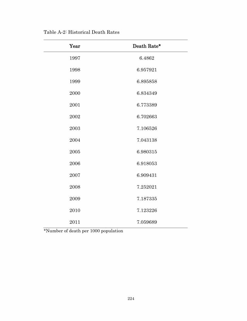
224
Table A-2: Historical Death Rates
Year Death Rate*
1997 6.4862
1998 6.957921
1999 6.895858
2000 6.834349
2001 6.773389
2002 6.702663
2003 7.106526
2004 7.043138
2005 6.980315
2006 6.918053
2007 6.909431
2008 7.252021
2009 7.187335
2010 7.123226
2011 7.059689
*Number of death per 1000 population

225
Table A-3: Historical Marriage Rates
Year Marriage Rate*
1981 7.8
1986 7.2
1991 6.4
1996 5.8
2001 5.3
2006 5.1
*Number of marriage per 1000 population

226
Table A-4: Historical In-migration Rates
Year In-migration Rate*
2001 42.43813
2002 42.0596
2003 41.68444
2004 41.31262
2005 40.94412
2006 42.65065
2007 42.27021
2008 41.89318
2009 41.5195
2010 41.14916
2011 40.74638
*Number of in-migration per 1000 households
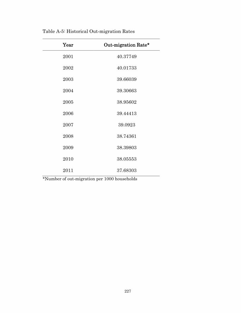
227
Table A-5: Historical Out-migration Rates
Year Out-migration Rate*
2001 40.37749
2002 40.01733
2003 39.66039
2004 39.30663
2005 38.95602
2006 39.44413
2007 39.0923
2008 38.74361
2009 38.39803
2010 38.05553
2011 37.68303
*Number of out-migration per 1000 households
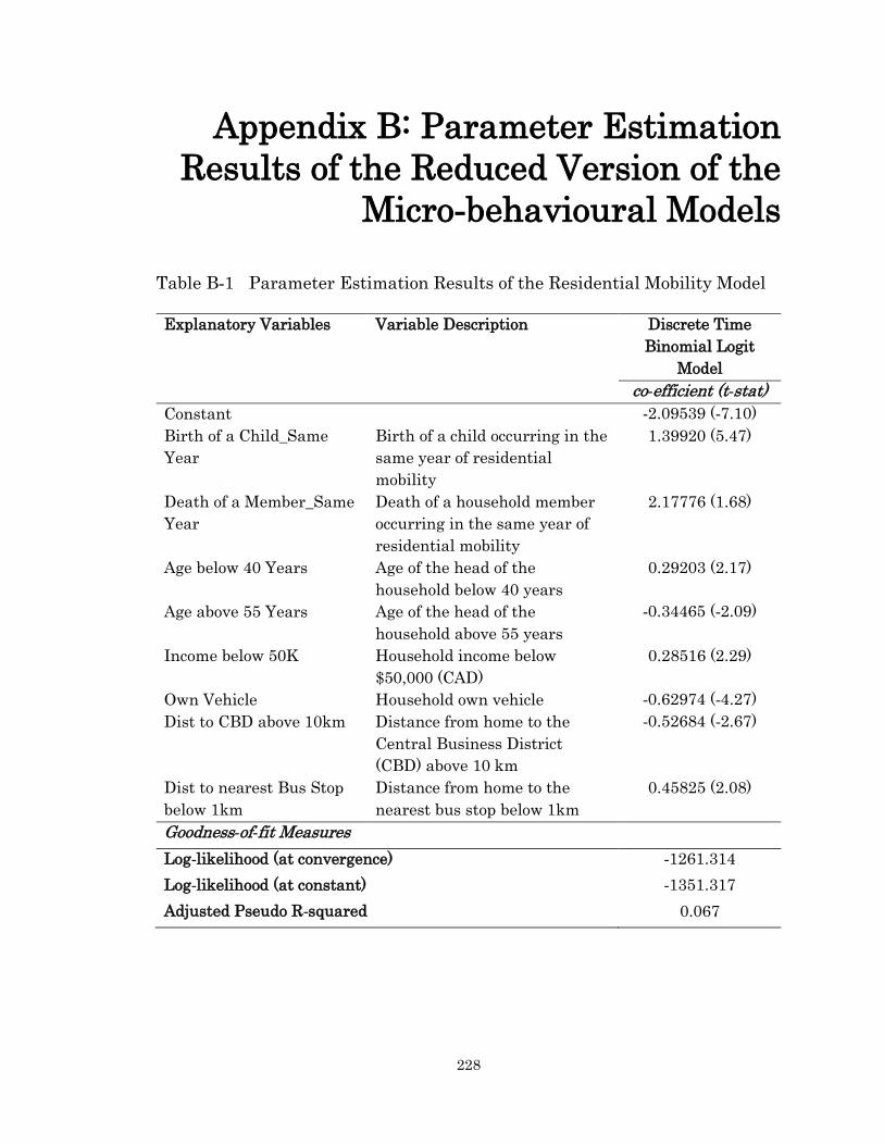
228
Appendix B: Parameter Estimation
Results of the Reduced Version of the
Micro-behavioural Models
Table B-1 Parameter Estimation Results of the Residential Mobility Model
Explanatory Variables Variable Description Discrete Time
Binomial Logit
Model
co-efficient (t-stat)
Constant -2.09539 (-7.10)
Birth of a Child_Same
Year
Birth of a child occurring in the
same year of residential
mobility
1.39920 (5.47)
Death of a Member_Same
Year
Death of a household member
occurring in the same year of
residential mobility
2.17776 (1.68)
Age below 40 Years Age of the head of the
household below 40 years
0.29203 (2.17)
Age above 55 Years Age of the head of the
household above 55 years
-0.34465 (-2.09)
Income below 50K Household income below
$50,000 (CAD)
0.28516 (2.29)
Own Vehicle Household own vehicle -0.62974 (-4.27)
Dist to CBD above 10km Distance from home to the
Central Business District
(CBD) above 10 km
-0.52684 (-2.67)
Dist to nearest Bus Stop
below 1km
Distance from home to the
nearest bus stop below 1km
0.45825 (2.08)
Goodness-of-fit Measures
Log-likelihood (at convergence) -1261.314
Log-likelihood (at constant) -1351.317
Adjusted Pseudo R-squared 0.067

229
Table B-2 Parameter Estimation Results of the Residential Location Choice
Model
Explanatory Variables Variable Description Multinomial Logit
Model
co-efficient (t-stat)
Parcel Size x Birth of a
Child_Same Year
Size of the property (acres)
interacted with birth of a child
occurring at the same year of
residential relocation
0.07882 (1.93)
Dist to CBD x Birth of a
Child_Same Year
Distance from home to the
Central Business District
(CBD) in km interacted with
birth of a child occurring at the
same year of residential
relocation
-0.02511 (-2.38)
Dist to CBD x No Car
Ownership
Distance from home to the
Central Business District
(CBD) in km interacted with
household not owning vehicle
-0.17151 (-2.34)
Dist to nearest Business
Center
Distance from home to the
nearest regional business
center in km
-0.13655 (-3.64)
Dist to nearest Business
Center x Single-detached
Distance from home to the
nearest regional business
center in km interacted with
household residing in single-
detached dwelling
0.16206 (4.14)
Dist to nearest School x
Presence of Children
Distance from home to the
nearest school in km interacted
with presence of children in the
household
-0.11315 (-1.90)
Dist to nearest Bus Stop Distance from home to the
nearest bus stop in km
-0.02395 (-2.07)
Dist to nearest Park Area Distance from home to the
nearest park area in km
-0.10128 (-1.47)
Population Density Population per acre area in the
home dissemination area
0.00013 (5.34)
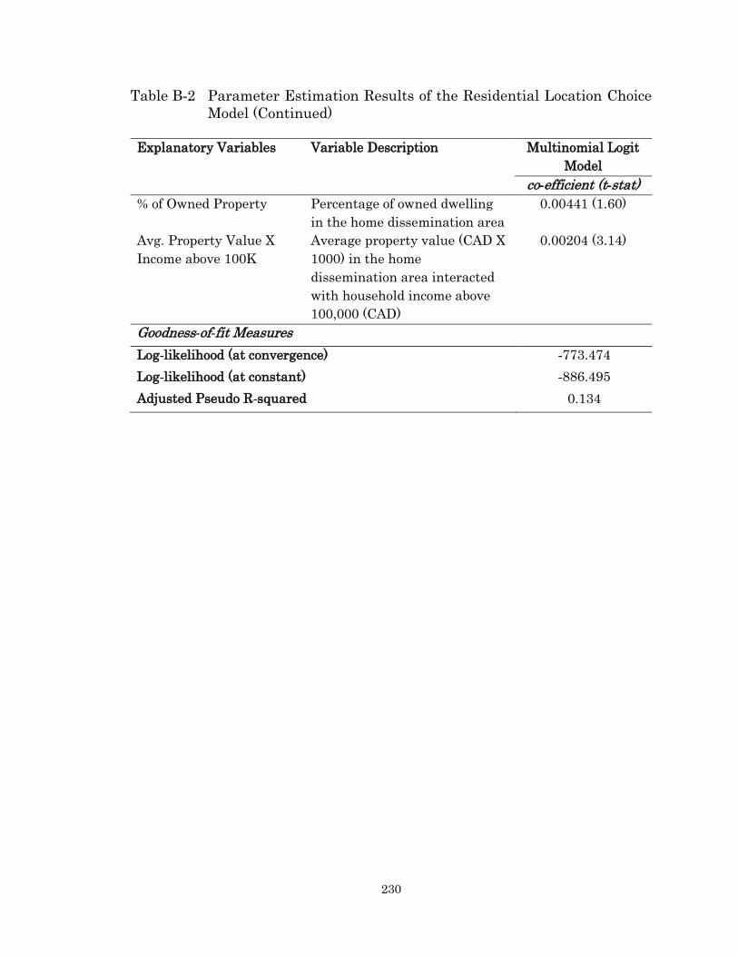
230
Table B-2 Parameter Estimation Results of the Residential Location Choice
Model (Continued)
Explanatory Variables Variable Description Multinomial Logit
Model
co-efficient (t-stat)
% of Owned Property Percentage of owned dwelling
in the home dissemination area
0.00441 (1.60)
Avg. Property Value X
Income above 100K
Average property value (CAD X
1000) in the home
dissemination area interacted
with household income above
100,000 (CAD)
0.00204 (3.14)
Goodness-of-fit Measures
Log-likelihood (at convergence) -773.474
Log-likelihood (at constant) -886.495
Adjusted Pseudo R-squared 0.134

231
Table B-3 Parameter Estimation Results of the First Time Vehicle Purchase
Model
Explanatory Variables Variable Description Discrete Time
Binomial Logit
Model
co-efficient (t-stat)
Constant Constant -3.44912 (-8.71)
Household
Formation_Same Year
First time vehicle purchase and
household formation occurring
in the same calendar year
-1.43051 (-1.31)
Residential Move_Same
Year
First time vehicle purchase and
residential relocation occurring
in the same calendar year
0.29572 (1.00)
Age below 30 Years Age of the head of the
household below 30 years
1.09653 (3.09)
Age between 30 to 40
Years
Age of the head of the
household between 30 to 40
years
1.10918 (3.33)
Income above 100k Household income above
$100,000(CAD)
0.72391 (3.12)
Household Size less than
4
Number of persons in the
household less than 4
0.65059 (2.60)
Owned Dwelling Household residing in owned
dwelling
0.98089 (2.96)
Single-detached Dwelling Household residing in single-
detached dwelling
-0.92243 (-3.40)
Goodness-of-fit Measures
Log-likelihood (at convergence) -348.908
Log-likelihood (at constant) -367.336
Adjusted Pseudo R-squared 0.050

232
Table B-4 Parameter Estimation Results of the Transaction or Do Nothing
Model
Explanatory Variables Variable Description Discrete Time Binomial
Logit Model
co-efficient (t-stat)
Constant Constant -1.97879 (-9.96)
Household
Formation_Same Year
Vehicle transaction and
household formation
occurring in the same
calendar year
-1.19280 (-1.60)
Residential Move_Same
Year
Vehicle transaction and
residential relocation
occurring in the same
calendar year
0.23221 (1.20)
Age below 30 Years Age of the head of the
household below 30 years
0.18306 (1.74)
Age above 50 Years Age of the head of the
household above 50 years
0.33636 (1.61)
Income above 100k Household income above
$100,000(CAD)
0.34737 (3.31)
Household Size less than
4
Number of persons in the
household less than 4
0.25415 (2.33)
Dist to nearest Bus Stop
less than 1km
Distance from home to
the nearest bus stop less
than 1 Km
0.21895 (1.91)
Dist to nearest School
less than 3 km
Distance from home to
the nearest school less
than 3 km
-0.34588 (-1.86)
Goodness-of-fit Measures
Log-likelihood (at convergence) -1445.404
Log-likelihood (at constant) -1460.900
Adjusted Pseudo R-squared 0.011
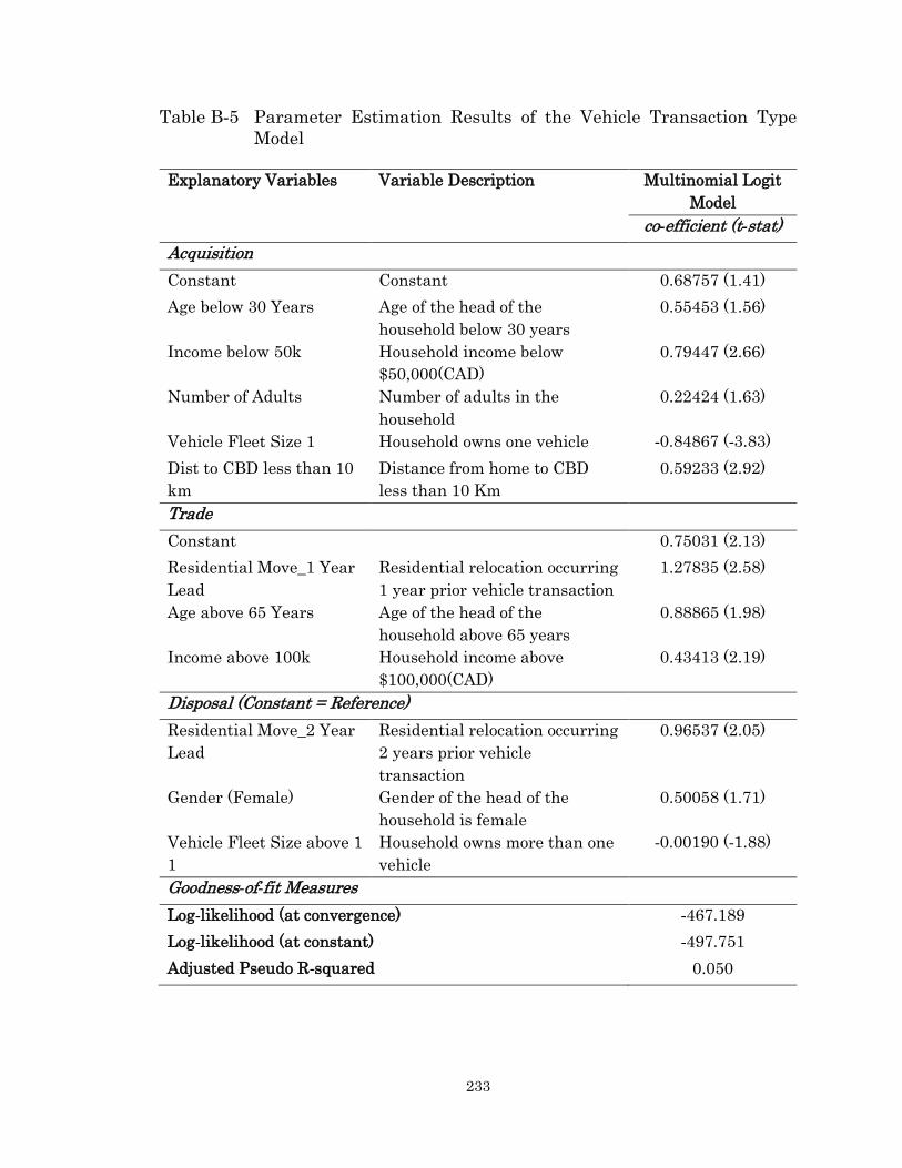
233
Table B-5 Parameter Estimation Results of the Vehicle Transaction Type
Model
Explanatory Variables Variable Description Multinomial Logit
Model
co-efficient (t-stat)
Acquisition
Constant Constant 0.68757 (1.41)
Age below 30 Years Age of the head of the
household below 30 years
0.55453 (1.56)
Income below 50k Household income below
$50,000(CAD)
0.79447 (2.66)
Number of Adults Number of adults in the
household
0.22424 (1.63)
Vehicle Fleet Size 1 Household owns one vehicle -0.84867 (-3.83)
Dist to CBD less than 10
km
Distance from home to CBD
less than 10 Km
0.59233 (2.92)
Trade
Constant 0.75031 (2.13)
Residential Move_1 Year
Lead
Residential relocation occurring
1 year prior vehicle transaction
1.27835 (2.58)
Age above 65 Years Age of the head of the
household above 65 years
0.88865 (1.98)
Income above 100k Household income above
$100,000(CAD)
0.43413 (2.19)
Disposal (Constant = Reference)
Residential Move_2 Year
Lead
Residential relocation occurring
2 years prior vehicle
transaction
0.96537 (2.05)
Gender (Female) Gender of the head of the
household is female
0.50058 (1.71)
Vehicle Fleet Size above 1
1
Household owns more than one
vehicle
-0.00190 (-1.88)
Goodness-of-fit Measures
Log-likelihood (at convergence) -467.189
Log-likelihood (at constant) -497.751
Adjusted Pseudo R-squared 0.050
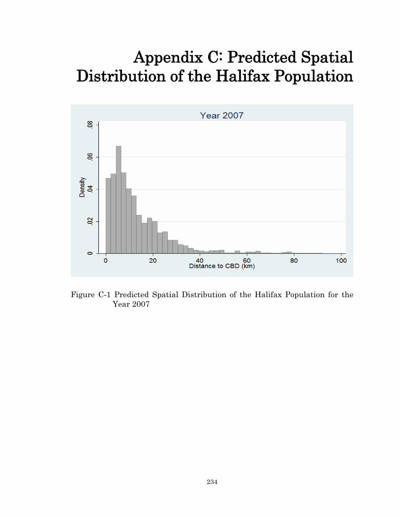
234
Appendix C: Predicted Spatial
Distribution of the Halifax Population
Figure C-1 Predicted Spatial Distribution of the Halifax Population for the
Year 2007

235
Figure C-2 Predicted Spatial Distribution of the Halifax Population for the
Year 2008
Figure C-3 Predicted Spatial Distribution of the Halifax Population for the
Year 2009
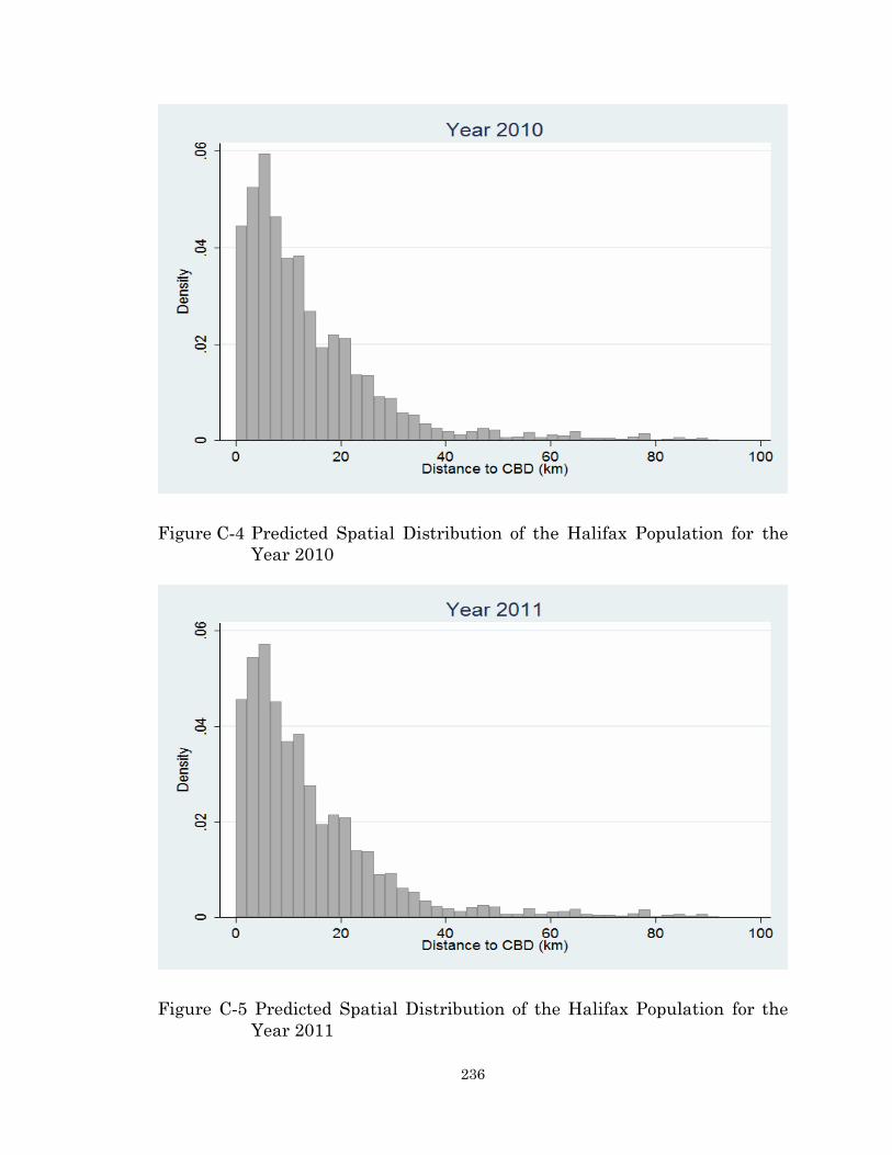
236
Figure C-4 Predicted Spatial Distribution of the Halifax Population for the
Year 2010
Figure C-5 Predicted Spatial Distribution of the Halifax Population for the
Year 2011
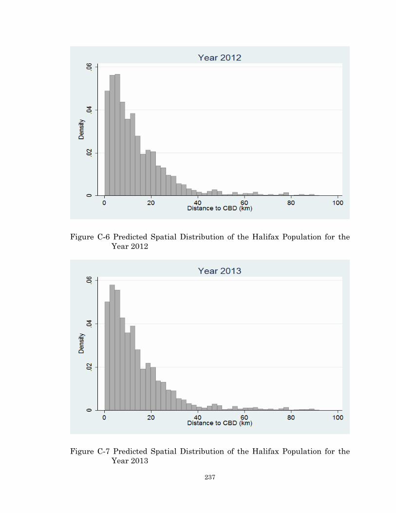
237
Figure C-6 Predicted Spatial Distribution of the Halifax Population for the
Year 2012
Figure C-7 Predicted Spatial Distribution of the Halifax Population for the
Year 2013
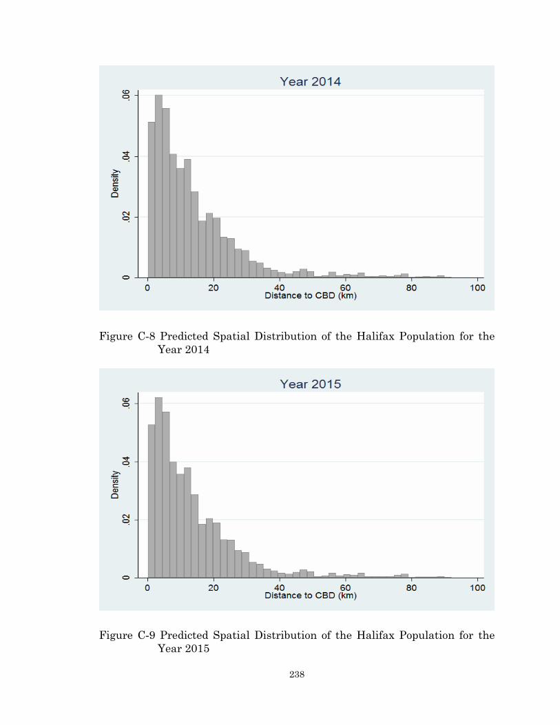
238
Figure C-8 Predicted Spatial Distribution of the Halifax Population for the
Year 2014
Figure C-9 Predicted Spatial Distribution of the Halifax Population for the
Year 2015
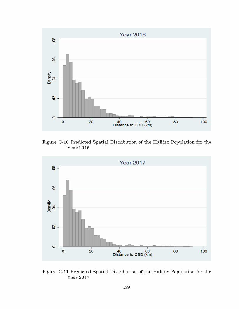
239
Figure C-10 Predicted Spatial Distribution of the Halifax Population for the
Year 2016
Figure C-11 Predicted Spatial Distribution of the Halifax Population for the
Year 2017

240
Figure C-12 Predicted Spatial Distribution of the Halifax Population for the
Year 2018
Figure C-13 Predicted Spatial Distribution of the Halifax Population for the
Year 2019
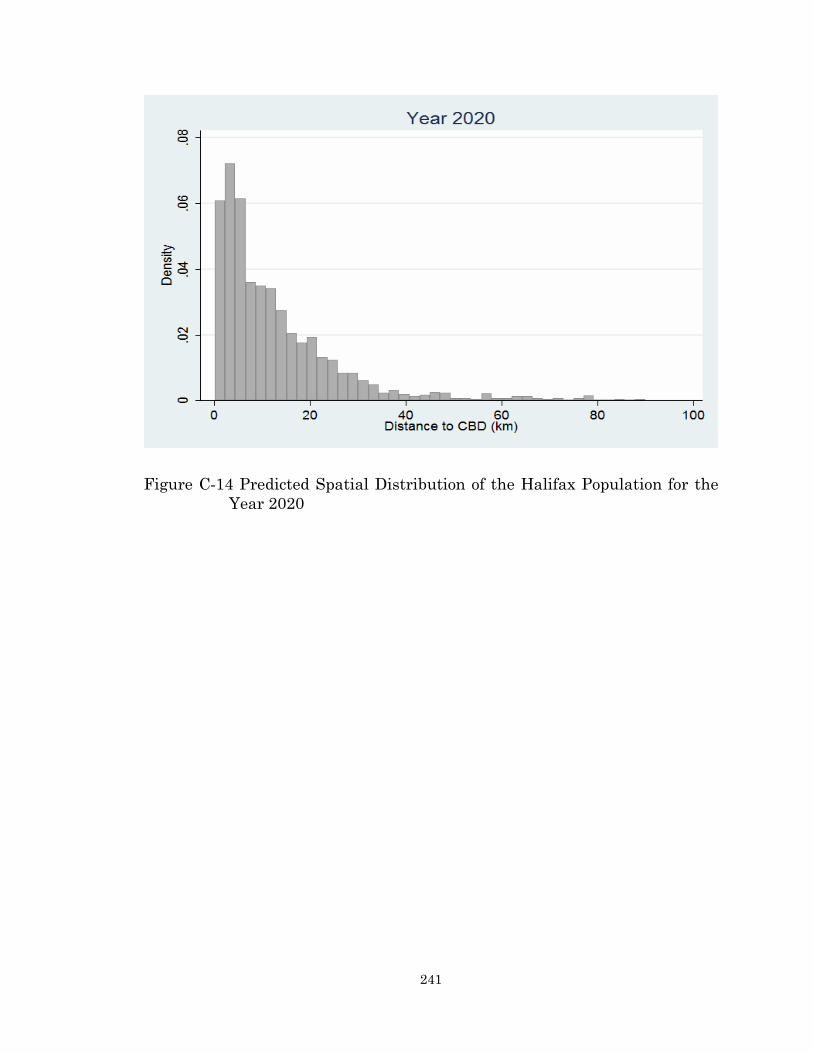
241
Figure C-14 Predicted Spatial Distribution of the Halifax Population for the
Year 2020
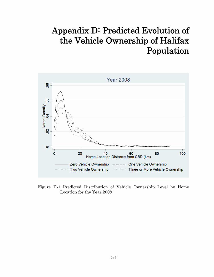
242
Appendix D: Predicted Evolution of
the Vehicle Ownership of Halifax
Population
Figure D-1 Predicted Distribution of Vehicle Ownership Level by Home
Location for the Year 2008

243
Figure D-2 Predicted Distribution of Vehicle Ownership Level by Home
Location for the Year 2009
Figure D-3 Predicted Distribution of Vehicle Ownership Level by Home
Location for the Year 2010
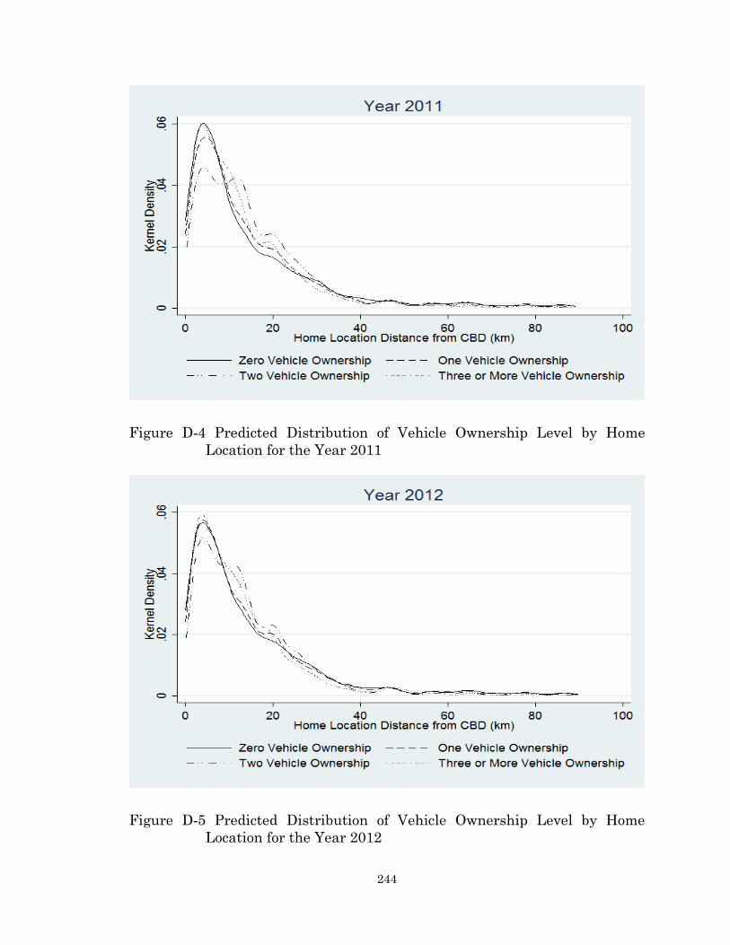
244
Figure D-4 Predicted Distribution of Vehicle Ownership Level by Home
Location for the Year 2011
Figure D-5 Predicted Distribution of Vehicle Ownership Level by Home
Location for the Year 2012

245
Figure D-6 Predicted Distribution of Vehicle Ownership Level by Home
Location for the Year 2013
Figure D-7 Predicted Distribution of Vehicle Ownership Level by Home
Location for the Year 2014
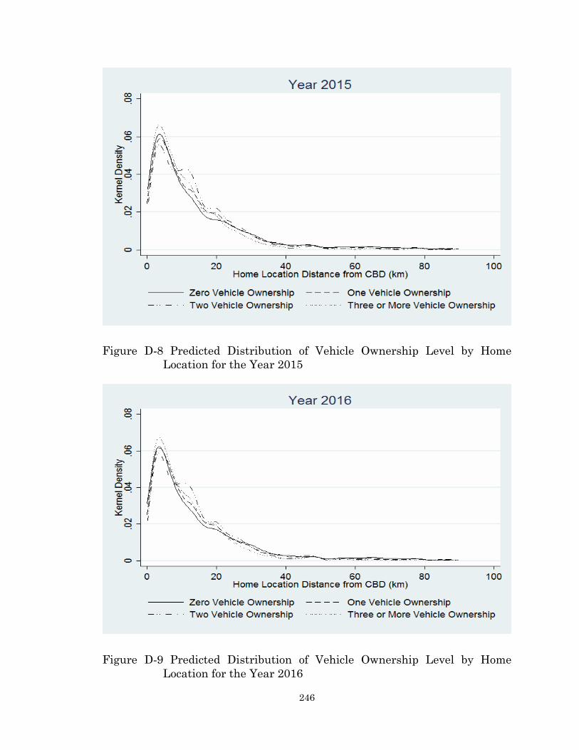
246
Figure D-8 Predicted Distribution of Vehicle Ownership Level by Home
Location for the Year 2015
Figure D-9 Predicted Distribution of Vehicle Ownership Level by Home
Location for the Year 2016
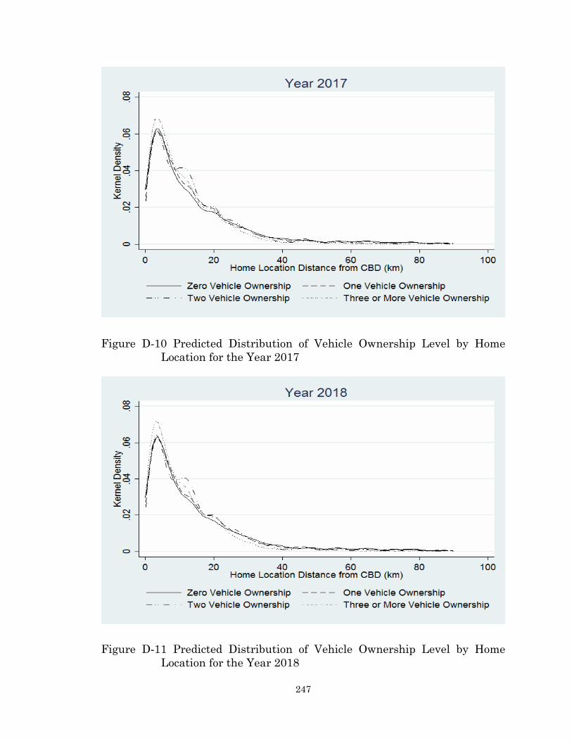
247
Figure D-10 Predicted Distribution of Vehicle Ownership Level by Home
Location for the Year 2017
Figure D-11 Predicted Distribution of Vehicle Ownership Level by Home
Location for the Year 2018
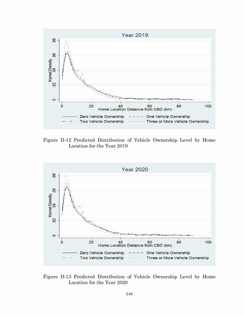
248
Figure D-12 Predicted Distribution of Vehicle Ownership Level by Home
Location for the Year 2019
Figure D-13 Predicted Distribution of Vehicle Ownership Level by Home
Location for the Year 2020

249
Figure D-14 Predicted Distribution of Vehicle Ownership Level by Home
Location for the Year 2021