Fault Classification of Power Distribution Cables by

2016 IEEE TRANSACTIONS ON INSTRUMENTATION AND MEASUREMENT, VOL. 69, NO. 5, MAY 2020

Fault Classification of Power Distribution Cablesby Detecting Decaying DC Components

With Magnetic SensingKe Zhu and Philip W. T. Pong

Abstract— Fault classification of power distribution cables isessential for tripping relays, pinpointing fault location, andrepairing failures of a distribution network in the power system.However, existing fault-classification techniques are not totallysatisfactory because they may: 1) require the precalibration ofresponding threshold for each network; 2) fail to identify thethree-phase short-circuit faults. since some electrical parameters(e.g., phase angle) are still symmetrical even in abnormal status;and 3) be invulnerable of electromagnetic interferences. In thispaper, a fault-classification technique by detecting decayingdc components of currents in faulted phases through magneticsensing is proposed to overcome the shortcomings mentionedabove. First, the three-phase currents are reconstructed bymagnetic sensing with a stochastic optimization algorithm, whichavoids the waveform distortion in the measurement by currenttransformers that incurred by the dc bias. Then, the dc compo-nent is extracted by mathematical morphology (MM) in phasecurrents to identify the fault type together with the polarity ofdc components. This method was verified successfully for variousfault types on a 22-kV power distribution cable in simulationand also a scaled power distribution network experimentally.The proposed method can enhance the reliability of the powerdistribution network and contribute to smart grid development.

Index Terms— DC component, fault classification, magneticsensing, power distribution cable, smart grid.

I. INTRODUCTION

ARELIABLE power distribution system is crucial forensuring the reliability and stability of electricity deliv-

ery to customers [1], [2]. Power distribution cables aretypically deployed underground instead of being overheadbecause this layout makes them less susceptible to outagesunder harsh weather conditions (e.g., high wind thunder-storms, heavy snow, and ice storms) and for the sake ofaesthetic purpose [3]. However, short-circuit faults still occur

Manuscript received January 18, 2019; revised May 18, 2019; acceptedMay 30, 2019. Date of publication June 12, 2019; date of current versionApril 7, 2020. This work was supported by the Seed Funding Program forBasic Research, Seed Funding Program for Applied Research and SmallProject Funding Program from the University of Hong Kong, ITF Tier 3funding under Grant ITS/203/14, Grant ITS/104/13, and Grant ITS/214/14,in part by RGC-GRF under Grant HKU 17210014 and Grant HKU 17204617,and in part by the University Grants Committee of Hong Kong under ContractAoE/P-04/08. The Associate Editor coordinating the review process wasGuglielmo Frigo. (Corresponding author: Philip W. T. Pong.)

The authors are with the Department of Electrical and Electronic Engi-neering, The University of Hong Kong, Hong Kong (e-mail: [email protected];[email protected]).

Color versions of one or more of the figures in this article are availableonline at http://ieeexplore.ieee.org.

Digital Object Identifier 10.1109/TIM.2019.2922514

on power distribution networks due to internal insulationbreakdown or external damage. For example, a screeningfault is an insulation breakdown that results in the physicalcontact between phase conductors and the screen [4]. As thescreen is grounded, a phase-to-ground fault occurs. The insu-lation between conductors can breakdown due to corrosion,leading to a phase-to-phase short-circuit fault. It would be aphase-phase-to-ground short-circuit fault if the screening isalso involved. An accidental excavation on the undergroundpower cable can lead to a three-phase short-circuit fault andan explosion as well [5]. The consequence of short-circuitfaults can be very serious. First, the excessive heating of thecables can result in fire and explosion. Moreover, a cascadetripping or shutdown can happen in a power system. As such,the short-circuit fault should be cleared up by relays withinthe shortest time to reduce the adverse effects.

To trip relays properly, a very critical step after detectingthe short-circuit fault is to classify its type [6], [7]. Thisis because the corresponding protection scheme should beexecuted immediately to clear the fault, minimize the effects,and recover the system. For example, a single-phase reclosingis executed to trip and reclose the faulted phase for extin-guishing the arcs and recovering the systems, rather than totrip irrelevant phases. The short-circuit fault type can also beused to infer the cause of faults. Therefore, an accurate andreliable fault classification for clearing and analyzing the faultsin the power system is significant.

Though a series of fault-classification techniques has beenproposed so far, these methods [8]–[12] suffer some problemsas summarized in Table I. First, most of the techniques requireprecalibration for responding threshold, which accounts for30% of the total capital cost of the workforce on settingrelay thresholds [13], [14]. For example, the threshold is setas a larger number (e.g., 1.5 times) as the steady currentin the overcurrent method [15], [16]. This cost is becomingincreasingly daunting when the electricity consumption andpower distribution network are drastically expanding overthe world [17]. Moreover, some of these techniques may bevulnerable to electromagnetic interference (EMI) from thebackground. This may lead to the erroneous fault classificationthat is attributable to the electromagnetic coupling between thefaulted and healthy phases [18]. This problem can becomeeven more severe with a larger number of high-frequencyelectronic devices used nearby nowadays. Besides, the

0018-9456 © 2019 IEEE. Personal use is permitted, but republication/redistribution requires IEEE permission.See https://www.ieee.org/publications/rights/index.html for more information.

Authorized licensed use limited to: The University of Hong Kong Libraries. Downloaded on November 25,2020 at 09:44:18 UTC from IEEE Xplore. Restrictions apply.

https://orcid.org/0000-0002-0157-8969

https://orcid.org/0000-0002-5554-8386

ZHU AND PONG: FAULT CLASSIFICATION OF POWER DISTRIBUTION CABLES 2017

TABLE I

ANALYSIS OF EXISTING FAULT-CLASSIFICATION METHODS

accuracy of fault classification needs improvement for iden-tifying the three-phase short-circuit fault. Some techniquesin Table I fail to identify such fault, because some electricalparameters (e.g., phase angle) in three-phase short-circuit faultremain symmetrical even in abnormal status. Therefore, a newfault-classification technique is necessary to overcome theseproblems [19], [20].

In this paper, a fault-classification technique by detectingdecaying dc components in fault currents with magnetic sens-ing is proposed, which overcomes the problems mentionedabove. In Section II, the analysis of dc component in powerdistribution networks and the process of extracting dc compo-nents from phase currents based on the magnetic sensing arepresented. The method is verified by simulation in Section III,and also by experiment in Section IV. The conclusion andfuture work are drawn in Section V.

II. METHODOLOGY

The dc component arises in the faulty phase when the short-circuit fault occurs. The analysis of dc components for thepower distribution network and the process of extracting thedc components of phase current from magnetic sensing arepresent as follows.

A. DC Component in Fault Currents

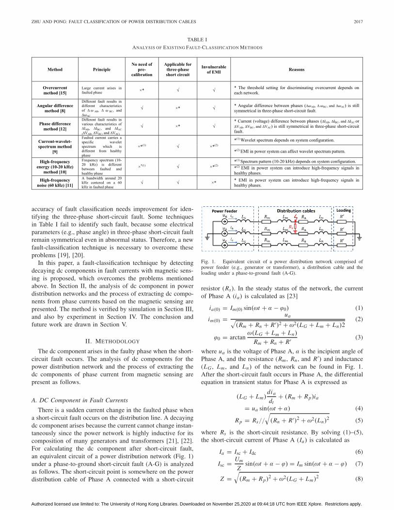
There is a sudden current change in the faulted phase whena short-circuit fault occurs on the distribution line. A decayingdc component arises because the current cannot change instan-taneously since the power network is highly inductive for itscomposition of many generators and transformers [21], [22].For calculating the dc component after short-circuit fault,an equivalent circuit of a power distribution network (Fig. 1)under a phase-to-ground short-circuit fault (A-G) is analyzedas follows. The short-circuit point is somewhere on the powerdistribution cable of Phase A connected with a short-circuit

Fig. 1. Equivalent circuit of a power distribution network comprised ofpower feeder (e.g., generator or transformer), a distribution cable and theloading under a phase-to-ground fault (A-G).

resistor (Rs). In the steady status of the network, the currentof Phase A (ia) is calculated as [23]

ia(0) = Im(0) sin(ωt + α − ϕ0) (1)

im(0) = ua√(Rm + Rn + R�)2 + ω2(LG + Lm + Ln)2

(2)

ϕ0 = arctanω(LG + Lm + Ln)

Rm + Rn + R� (3)

where ua is the voltage of Phase A, α is the incipient angle ofPhase A, and the resistance (Rm , Rn , and R�) and inductance(LG , Lm , and Ln) of the network can be found in Fig. 1.After the short-circuit fault occurs in Phase A, the differentialequation in transient status for Phase A is expressed as

(LG + Lm)dia

dt+ (Rm + Rp)ia

= ua sin(ωt + α) (4)

Rp = Rs//

√(Rn + R�)2 + ω2(Ln)2 (5)

where Rs is the short-circuit resistance. By solving (1)–(5),the short-circuit current of Phase A (Ia) is calculated as

Ia = Isc + Idc (6)

Isc = Um

Zsin(ωt + α − ϕ) = Im sin(ωt + α − ϕ) (7)

Z =√

(Rm + Rp)2 + ω2(LG + Lm)2 (8)



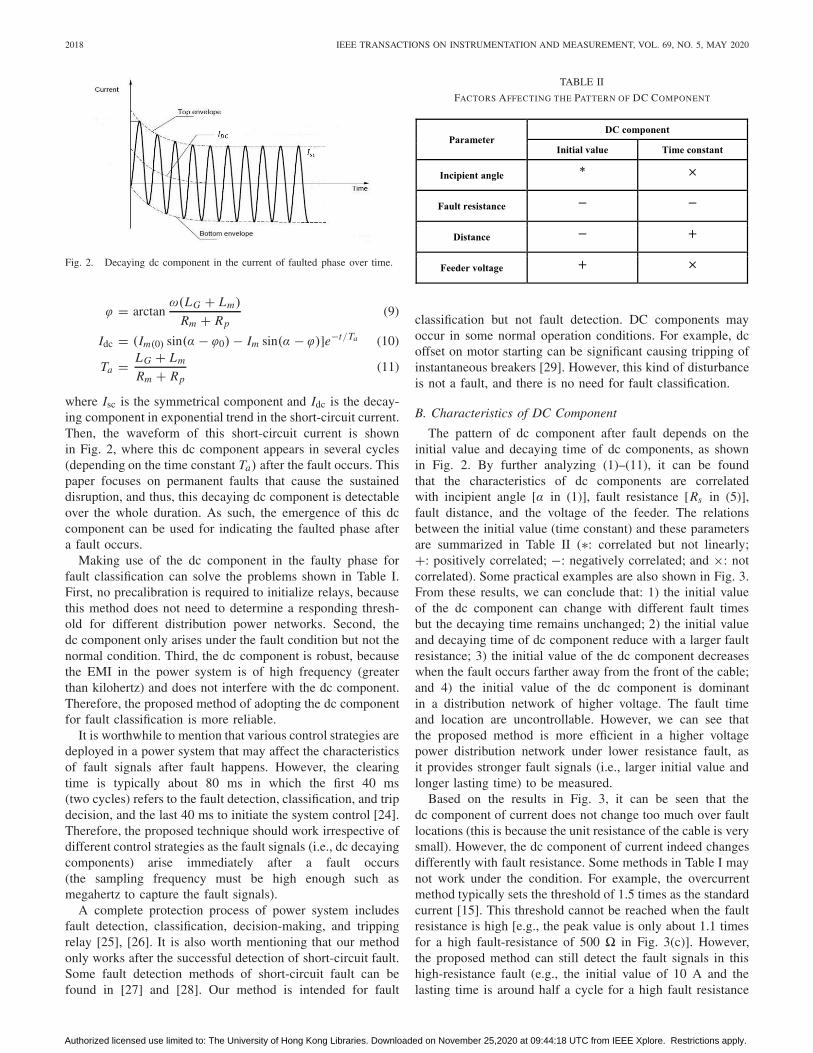
Fig. 2. Decaying dc component in the current of faulted phase over time.

ϕ = arctanω(LG + Lm)

Rm + Rp(9)

Idc = (Im(0) sin(α − ϕ0) − Im sin(α − ϕ)]e−t/Ta (10)

Ta = LG + Lm

Rm + Rp(11)

where Isc is the symmetrical component and Idc is the decay-ing component in exponential trend in the short-circuit current.Then, the waveform of this short-circuit current is shownin Fig. 2, where this dc component appears in several cycles(depending on the time constant Ta) after the fault occurs. Thispaper focuses on permanent faults that cause the sustaineddisruption, and thus, this decaying dc component is detectableover the whole duration. As such, the emergence of this dccomponent can be used for indicating the faulted phase aftera fault occurs.

Making use of the dc component in the faulty phase forfault classification can solve the problems shown in Table I.First, no precalibration is required to initialize relays, becausethis method does not need to determine a responding thresh-old for different distribution power networks. Second, thedc component only arises under the fault condition but not thenormal condition. Third, the dc component is robust, becausethe EMI in the power system is of high frequency (greaterthan kilohertz) and does not interfere with the dc component.Therefore, the proposed method of adopting the dc componentfor fault classification is more reliable.

It is worthwhile to mention that various control strategies aredeployed in a power system that may affect the characteristicsof fault signals after fault happens. However, the clearingtime is typically about 80 ms in which the first 40 ms(two cycles) refers to the fault detection, classification, and tripdecision, and the last 40 ms to initiate the system control [24].Therefore, the proposed technique should work irrespective ofdifferent control strategies as the fault signals (i.e., dc decayingcomponents) arise immediately after a fault occurs(the sampling frequency must be high enough such asmegahertz to capture the fault signals).

A complete protection process of power system includesfault detection, classification, decision-making, and trippingrelay [25], [26]. It is also worth mentioning that our methodonly works after the successful detection of short-circuit fault.Some fault detection methods of short-circuit fault can befound in [27] and [28]. Our method is intended for fault

TABLE II

FACTORS AFFECTING THE PATTERN OF DC COMPONENT

classification but not fault detection. DC components mayoccur in some normal operation conditions. For example, dcoffset on motor starting can be significant causing tripping ofinstantaneous breakers [29]. However, this kind of disturbanceis not a fault, and there is no need for fault classification.

B. Characteristics of DC Component

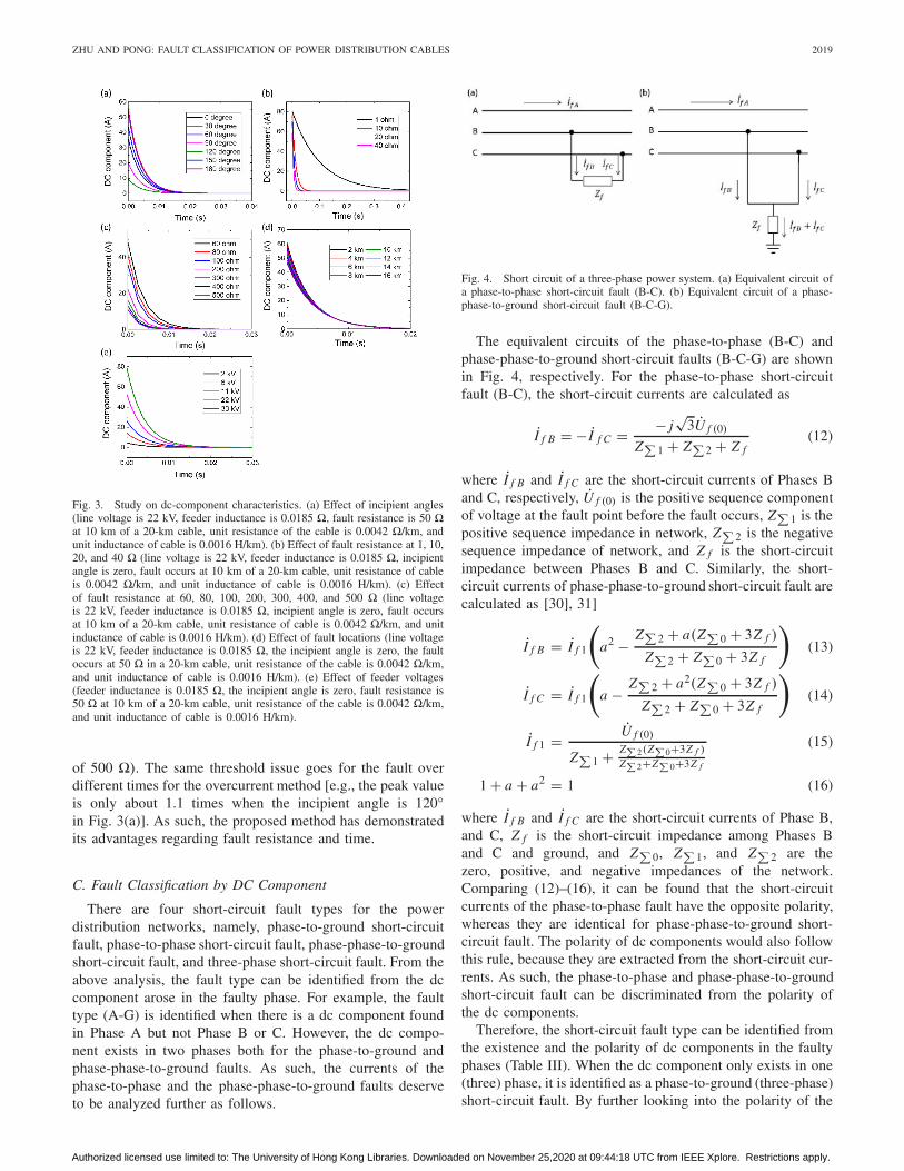
The pattern of dc component after fault depends on theinitial value and decaying time of dc components, as shownin Fig. 2. By further analyzing (1)–(11), it can be foundthat the characteristics of dc components are correlatedwith incipient angle [α in (1)], fault resistance [Rs in (5)],fault distance, and the voltage of the feeder. The relationsbetween the initial value (time constant) and these parametersare summarized in Table II (∗: correlated but not linearly;+: positively correlated; −: negatively correlated; and ×: notcorrelated). Some practical examples are also shown in Fig. 3.From these results, we can conclude that: 1) the initial valueof the dc component can change with different fault timesbut the decaying time remains unchanged; 2) the initial valueand decaying time of dc component reduce with a larger faultresistance; 3) the initial value of the dc component decreaseswhen the fault occurs farther away from the front of the cable;and 4) the initial value of the dc component is dominantin a distribution network of higher voltage. The fault timeand location are uncontrollable. However, we can see thatthe proposed method is more efficient in a higher voltagepower distribution network under lower resistance fault, asit provides stronger fault signals (i.e., larger initial value andlonger lasting time) to be measured.

Based on the results in Fig. 3, it can be seen that thedc component of current does not change too much over faultlocations (this is because the unit resistance of the cable is verysmall). However, the dc component of current indeed changesdifferently with fault resistance. Some methods in Table I maynot work under the condition. For example, the overcurrentmethod typically sets the threshold of 1.5 times as the standardcurrent [15]. This threshold cannot be reached when the faultresistance is high [e.g., the peak value is only about 1.1 timesfor a high fault-resistance of 500 � in Fig. 3(c)]. However,the proposed method can still detect the fault signals in thishigh-resistance fault (e.g., the initial value of 10 A and thelasting time is around half a cycle for a high fault resistance



Fig. 3. Study on dc-component characteristics. (a) Effect of incipient angles(line voltage is 22 kV, feeder inductance is 0.0185 �, fault resistance is 50 �at 10 km of a 20-km cable, unit resistance of the cable is 0.0042 �/km, andunit inductance of cable is 0.0016 H/km). (b) Effect of fault resistance at 1, 10,20, and 40 � (line voltage is 22 kV, feeder inductance is 0.0185 �, incipientangle is zero, fault occurs at 10 km of a 20-km cable, unit resistance of cableis 0.0042 �/km, and unit inductance of cable is 0.0016 H/km). (c) Effectof fault resistance at 60, 80, 100, 200, 300, 400, and 500 � (line voltageis 22 kV, feeder inductance is 0.0185 �, incipient angle is zero, fault occursat 10 km of a 20-km cable, unit resistance of cable is 0.0042 �/km, and unitinductance of cable is 0.0016 H/km). (d) Effect of fault locations (line voltageis 22 kV, feeder inductance is 0.0185 �, the incipient angle is zero, the faultoccurs at 50 � in a 20-km cable, unit resistance of the cable is 0.0042 �/km,and unit inductance of cable is 0.0016 H/km). (e) Effect of feeder voltages(feeder inductance is 0.0185 �, the incipient angle is zero, fault resistance is50 � at 10 km of a 20-km cable, unit resistance of the cable is 0.0042 �/km,and unit inductance of cable is 0.0016 H/km).

of 500 �). The same threshold issue goes for the fault overdifferent times for the overcurrent method [e.g., the peak valueis only about 1.1 times when the incipient angle is 120◦in Fig. 3(a)]. As such, the proposed method has demonstratedits advantages regarding fault resistance and time.

C. Fault Classification by DC Component

There are four short-circuit fault types for the powerdistribution networks, namely, phase-to-ground short-circuitfault, phase-to-phase short-circuit fault, phase-phase-to-groundshort-circuit fault, and three-phase short-circuit fault. From theabove analysis, the fault type can be identified from the dccomponent arose in the faulty phase. For example, the faulttype (A-G) is identified when there is a dc component foundin Phase A but not Phase B or C. However, the dc compo-nent exists in two phases both for the phase-to-ground andphase-phase-to-ground faults. As such, the currents of thephase-to-phase and the phase-phase-to-ground faults deserveto be analyzed further as follows.

Fig. 4. Short circuit of a three-phase power system. (a) Equivalent circuit ofa phase-to-phase short-circuit fault (B-C). (b) Equivalent circuit of a phase-phase-to-ground short-circuit fault (B-C-G).

The equivalent circuits of the phase-to-phase (B-C) andphase-phase-to-ground short-circuit faults (B-C-G) are shownin Fig. 4, respectively. For the phase-to-phase short-circuitfault (B-C), the short-circuit currents are calculated as

I f B = − I f C = − j√

3U f (0)

Z∑1 + Z∑

2 + Z f(12)

where I f B and I f C are the short-circuit currents of Phases Band C, respectively, U f (0) is the positive sequence componentof voltage at the fault point before the fault occurs, Z∑

1 is thepositive sequence impedance in network, Z∑

2 is the negativesequence impedance of network, and Z f is the short-circuitimpedance between Phases B and C. Similarly, the short-circuit currents of phase-phase-to-ground short-circuit fault arecalculated as [30], 31]

I f B = I f 1

(a2 − Z∑

2 + a(Z∑0 + 3Z f )

Z∑2 + Z∑

0 + 3Z f

)(13)

I f C = I f 1

(a − Z∑

2 + a2(Z∑0 + 3Z f )

Z∑2 + Z∑

0 + 3Z f

)(14)

I f 1 = U f (0)

Z∑1 + Z∑

2(Z∑0+3Z f )

Z∑2+Z∑

0+3Z f

(15)

1 + a + a2 = 1 (16)

where I f B and I f C are the short-circuit currents of Phase B,and C, Z f is the short-circuit impedance among Phases Band C and ground, and Z∑

0, Z∑1, and Z∑

2 are thezero, positive, and negative impedances of the network.Comparing (12)–(16), it can be found that the short-circuitcurrents of the phase-to-phase fault have the opposite polarity,whereas they are identical for phase-phase-to-ground short-circuit fault. The polarity of dc components would also followthis rule, because they are extracted from the short-circuit cur-rents. As such, the phase-to-phase and phase-phase-to-groundshort-circuit fault can be discriminated from the polarity ofthe dc components.

Therefore, the short-circuit fault type can be identified fromthe existence and the polarity of dc components in the faultyphases (Table III). When the dc component only exists in one(three) phase, it is identified as a phase-to-ground (three-phase)short-circuit fault. By further looking into the polarity of the



TABLE III

FAULT CLASSIFICATION BASED ON DC COMPONENTSIN SHORT-CIRCUIT CURRENTS

dc components, the phase-to-phase and phase-phase-to-groundshort-circuit fault can be discriminated.

D. Current Reconstruction From Magnetic Sensing

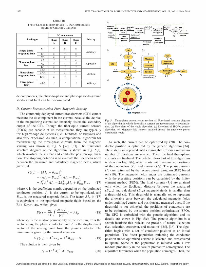
The commonly deployed current transformers (CTs) cannotmeasure the dc component in the current, because the dc biasin the magnetizing current can inversely distort the secondaryoutput of the CTs. Though the fiber-optic current sensors(FOCS) are capable of dc measurement, they are typicallyfor high-voltage dc systems (i.e., hundreds of kilovolt) andalso very expensive. As such, a computational algorithm forreconstructing the three-phase currents from the magneticsensing was shown in Fig. 5 [32], [33]. The functionalstructure diagram of the algorithm is shown in Fig. 5(a),which involves the current and conductor position optimiza-tion. The stopping criterion is to evaluate the Euclidean normbetween the measured and calculated magnetic fields, whichgives [34]

f (Ip) = �AIp − Bmea�2

= (AIp − Bmea)T (AIp − Bmea)

= I Tp AT AIp − 2BT

mea AIp + BTmea Bmea (17)

where A is the coefficient matrix depending on the optimizedconductor position, Ip is the current to be optimized, andBmea is the measured magnetic fields. The factor AIp in (17)is equivalent to the optimized magnetic fields based on theBiot–Savart law, which gives

B(r) = μr

4π

∫dl × r �

|r �|3 I = AIp (18)

where μr is the relative permeability of the medium, dl is thevector along the phase conductor, and r � is the displacementvector of the sensing point from the phase conductor. Theminimum is given by the normal equation

∇ f (Ip) = AT AIp − AT Bmea = 0. (19)

The solution is then given by

Ip = (AT A)−1

AT Bmea. (20)

Fig. 5. Three-phase current reconstruction. (a) Functional structure diagramof the algorithm in which three-phase currents are reconstructed via optimiza-tion. (b) Flow chart of the whole algorithm. (c) Flowchart of SPO by geneticalgorithm. (d) Magnetic-field sensors installed around the three-core powerdistribution cable.

As such, the current can be optimized by (20). The con-ductor position is optimized by the genetic algorithm [34].These steps are repeated until a reasonable error or a maximumnumber of iterations are reached. Then, the final three-phasecurrents are finalized. The detailed flowchart of this algorithmis shown in Fig. 5(b), which starts with preassumed positionsof the conductors (P0) and currents (I0). The phase currents(Ip) are optimized by the inverse current program (ICP) basedon (19). The magnetic fields under the optimized currentswith the presetting positions can be calculated by the finite-element method (FEM). The final currents (I f ) are attainedonly when the Euclidean distance between the measured(Bmea) and calculated (Bcal) magnetic fields is smaller thana threshold (ε). This threshold is manually set to representthe allowable error between the calculated magnetic fieldsunder optimized current and position and measured ones. If thethreshold is not achieved, the positions of conductors areto be optimized by the source position optimization (SPO).The SPO is embedded with the genetic algorithm, and itsdetails are shown in Fig. 5(c). The genetic algorithm is asearch heuristic that reflects the process of natural selection(i.e., selection, crossover, and mutation) [35], [36]. The algo-rithm begins with a set of conductor position as an initialpopulation. The fittest population reflecting the conductorposition under optimized current is selected and crossoveredto update. Some of the population is mutated with a lowrandom probability in the case of premature convergence. Thealgorithm terminates when the population converges. Then, the



fittest phase conductor is chosen for ICP to repeat the processuntil the threshold (ε) is satisfied. Finally, the three-phasecurrents are reconstructed from the magnetic fields.

The positions of phase conductors and phase currents needto be tuned in our program. The initial values are criticalfor achieving the best solutions in the iteration process [35].Regarding the initial position of three-phase conductors (P0),their phase differences are recommended to be set with120◦ differences, and be located in the middle between thecable center and the boundary. The initial currents (I0) areset around the rated value of the cable. The crossover rateis set large (e.g., >0.9) and the mutation rate must be low(e.g., <0.05) in SPO [35]. Moreover, the accuracy of thereconstructed result relies on the magnetic-field measure-ment [34]. The accuracy can be improved by increasing thenumber of sensing points [34]. In reality, the magnetic sensorsare installed circularly around the cable surface [Fig. 5(d)].Since magnetic sensors (e.g., low-cost magnetoresistive sen-sors) can operate from dc to over 1 MHz, the dc componentsof the three-phase currents can be preserved by this currentreconstruction method.

It is worthwhile to mention that the stochastic optimizationalgorithm only needs to operate when the phase currentsand conductor positions are unknown. After determining thepositions of phase conductors, the phase currents can bedirectly solved from the magnetic fields without runningthe stochastic program again. This step will not induce anyartificial dc components in the restored currents unless themagnetic sensors measure asymmetrical magnetic fields dueto the actual dc currents.

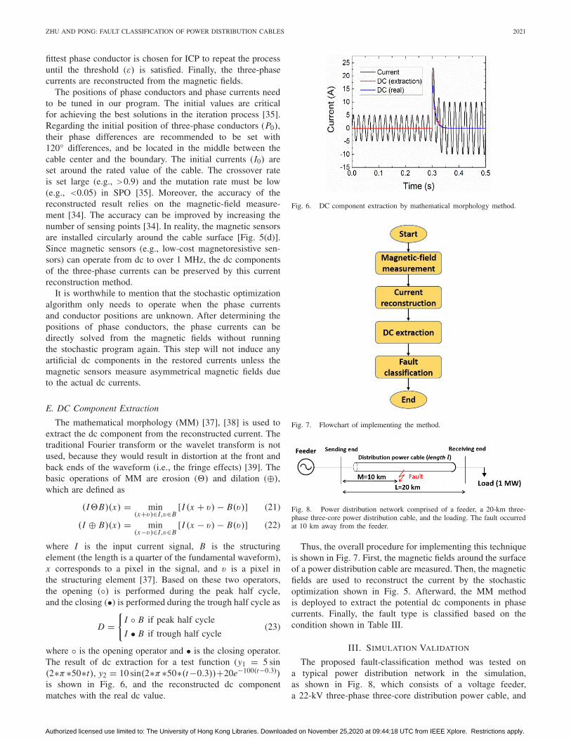
E. DC Component Extraction

The mathematical morphology (MM) [37], [38] is used toextract the dc component from the reconstructed current. Thetraditional Fourier transform or the wavelet transform is notused, because they would result in distortion at the front andback ends of the waveform (i.e., the fringe effects) [39]. Thebasic operations of MM are erosion (�) and dilation (⊕),which are defined as

(I�B)(x) = min(x+v)∈I,v∈B

[I (x + v) − B(v)] (21)

(I ⊕ B)(x) = min(x−v)∈I,v∈B

[I (x − v) − B(v)] (22)

where I is the input current signal, B is the structuringelement (the length is a quarter of the fundamental waveform),x corresponds to a pixel in the signal, and v is a pixel inthe structuring element [37]. Based on these two operators,the opening (◦) is performed during the peak half cycle,and the closing (•) is performed during the trough half cycle as

D ={

I ◦ B if peak half cycle

I • B if trough half cycle(23)

where ◦ is the opening operator and • is the closing operator.The result of dc extraction for a test function (y1 = 5 sin(2∗π∗50∗t), y2 = 10 sin(2∗π∗50∗(t−0.3))+20e−100(t−0.3))is shown in Fig. 6, and the reconstructed dc componentmatches with the real dc value.

Fig. 6. DC component extraction by mathematical morphology method.

Fig. 7. Flowchart of implementing the method.

Fig. 8. Power distribution network comprised of a feeder, a 20-km three-phase three-core power distribution cable, and the loading. The fault occurredat 10 km away from the feeder.

Thus, the overall procedure for implementing this techniqueis shown in Fig. 7. First, the magnetic fields around the surfaceof a power distribution cable are measured. Then, the magneticfields are used to reconstruct the current by the stochasticoptimization shown in Fig. 5. Afterward, the MM methodis deployed to extract the potential dc components in phasecurrents. Finally, the fault type is classified based on thecondition shown in Table III.

III. SIMULATION VALIDATION

The proposed fault-classification method was tested ona typical power distribution network in the simulation,as shown in Fig. 8, which consists of a voltage feeder,a 22-kV three-phase three-core distribution power cable, and



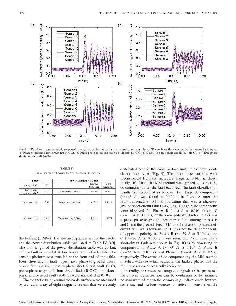
Fig. 9. Resultant magnetic fields measured around the cable surface by the magnetic sensors placed 60 mm from the cable center in various fault types.(a) Phase-to-ground short-circuit fault (A-G). (b) Phase-phase-to-ground short-circuit fault (B-C-G). (c) Phase-to-phase short-circuit fault (B-C). (d) Three-phaseshort-circuits fault (A-B-C).

TABLE IV

PARAMETER OF POWER DISTRIBUTION NETWORK

the loading (1 MW). The electrical parameters for the feederand the power distribution cable are listed in Table IV [40].The total length of the power distribution cable was 20 km,and the fault occurred at 10 km away from the feeder side. Thesensing platform was installed at the front end of the cable.Four short-circuit fault types, i.e., phase-to-ground short-circuit fault (A-G), phase-to-phase short-circuit fault (B-C),phase-phase-to-ground short-circuit fault (B-C-G), and three-phase short-circuit fault (A-B-C) were simulated at 0.10 s.

The magnetic fields around the cable surface were measuredby a circular array of eight magnetic sensors that were evenly

distributed around the cable surface under these four short-circuit fault types (Fig. 9). The three-phase currents werereconstructed from the measured magnetic fields, as shownin Fig. 10. Then, the MM method was applied to extract thedc component after the fault occurred. The fault-classificationresults are elaborated as follows: 1) a large dc component(∼+63 A) was found at 0.109 s in Phase A after thefault happened at 0.10 s, indicating this was a phase-to-ground short-circuit fault (A-G) [Fig. 10(a)]; 2) dc componentswere observed for Phases B (−46 A at 0.105 s) and C(∼−10 A at 0.102 s) of the same polarity, disclosing this wasa phase-phase-to-ground short-circuit fault among Phases Band C and the ground [Fig. 10(b)]; 3) the phase-to-phase short-circuit fault was shown in Fig. 10(c) since the dc componentsof opposite polarity in Phases B (∼−29 A at 0.104 s) andC (∼+26 A at 0.103 s) were seen; and 4) a three-phaseshort-circuit fault was shown in Fig. 10(d) by observing dccomponents in Phase A (∼+69 A at 0.109 s), Phase B(∼−64 A at 0.105 s), and Phase C (∼−20 A at 0.102 s),respectively. The extracted dc component by the MM methodmatched with the actual values in the faulted phases and thefault types were successfully indicated.

In reality, the measured magnetic signals to be processedfor current reconstruction can be contaminated by intrinsicnoises/errors of magnetic sensors (e.g., offset error, hystere-sis error, and various sources of noise in sensor) or the



Fig. 10. Reconstructed three-phase currents with the extracted and realdc component in various fault types. (a) Phase-to-ground short-circuit fault(A-G). (b) Phase-phase-to-ground short-circuit fault (B-C-G). (c) Phase-to-phase short-circuit fault (B-C). (d) Three-phase short-circuit fault (A-B-C).

Fig. 11. Influence of noise on current reconstruction. (a) Phase currentreconstructed from noisy magnetic-field measurement at SNR = 25. (b) Phasecurrent reconstructed from noisy magnetic-field measurement at SNR = 10.(c) Phase current reconstructed from noisy magnetic-field measurement atSNR = 5. (d) DC component extracted from the reconstructed phase currentbased on noisy magnetic-field measurement (SNR = 25, 10, and 5 dB).

background electromagnetic noises. To investigate the influ-ence of noises, signal-to-noise ratios at different levels(25–40-dB SNR represent very good signals, 15–25-dB SNRgood signals, 10–15-dB SNR low signals, and 5–10-dB SNRbad signals [41]) were added into the magnetic-field measure-ment in the steady status of the system configuration in Fig. 8.A cycle of phase current reconstructed from magnetic-fieldmeasurement under several noise levels (SNR = 25, 10,and 5 dB) is shown in Fig. 11. It can be seen that thereconstructed currents became more fluctuated as the noiselevel increased [Fig. 11(a)–(c)]. The extracted dc compo-nents also became stronger accordingly (0.43, 0.58, and 3.55,respectively), as shown in Fig. 11(d), because the asymmetry

Fig. 12. Experimental setup for validating the proposed fault-classificationmethod. (a) Schematic of the testing platform comprised of a programmablepower source, a power distribution cable, loadings, and a sensing platform.(b) Hardware of the testing platform.

Fig. 13. Magnetic field measurement. (a) Array of 16 magnetic sen-sors around the cable surface to measure y- and z-axes magnetic fields.(b) Hardware of sensing platform comprised of magnetic sensors, reset circuit,and magnetic shielding.

of current increased due to the noise. This will introducea dc component in the steady status of system operation,which can confuse the proposed method. Therefore, it isnecessary to eliminate the background magnetic disturbances(e.g., installing a magnetic shielding).

IV. EXPERIMENTAL VALIDATION AND DISCUSSION

The experiment was conducted in the lab to verify thepractical feasibility of the proposed method for the faultclassification of power distribution cables. The schematic ofthe experimental setup comprised of a power supply, a powerdistribution cable, a sensing platform, and the loadings isshown in Fig. 12(a). The power distribution cable was ener-gized by a programmable power source (61704, Chroma) andconnected with resistive loadings [Fig. 12(b)]. The voltage



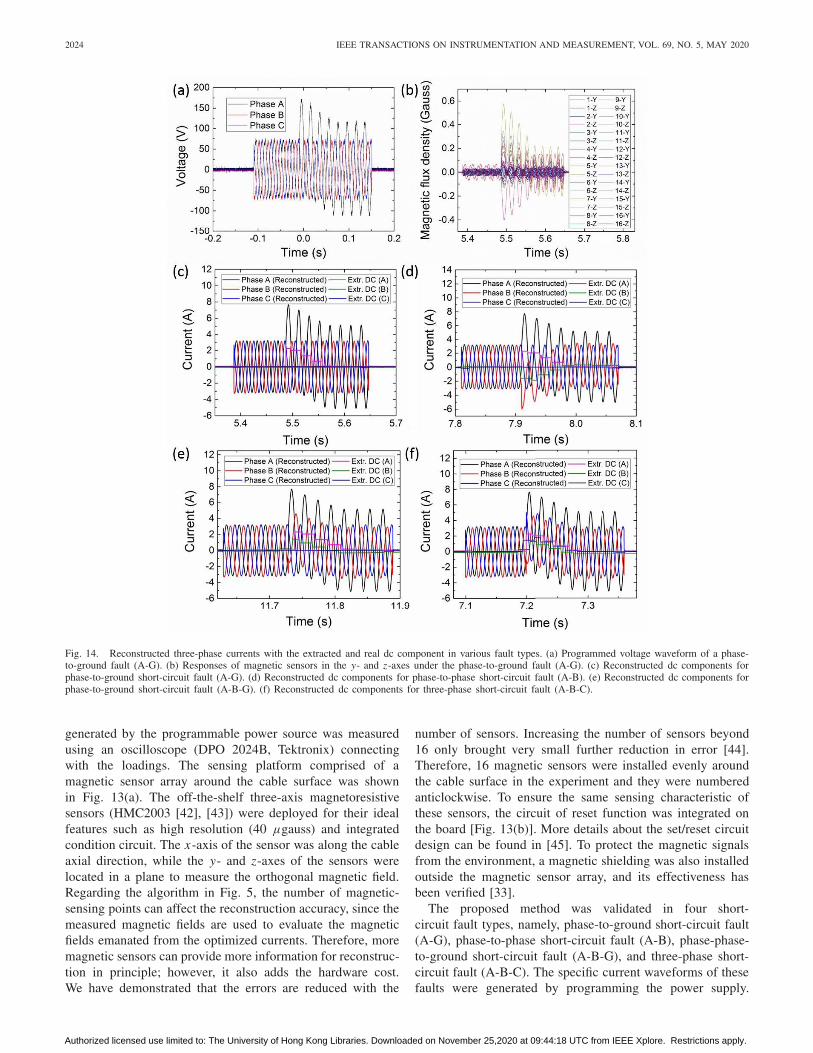
Fig. 14. Reconstructed three-phase currents with the extracted and real dc component in various fault types. (a) Programmed voltage waveform of a phase-to-ground fault (A-G). (b) Responses of magnetic sensors in the y- and z-axes under the phase-to-ground fault (A-G). (c) Reconstructed dc components forphase-to-ground short-circuit fault (A-G). (d) Reconstructed dc components for phase-to-phase short-circuit fault (A-B). (e) Reconstructed dc components forphase-to-ground short-circuit fault (A-B-G). (f) Reconstructed dc components for three-phase short-circuit fault (A-B-C).

generated by the programmable power source was measuredusing an oscilloscope (DPO 2024B, Tektronix) connectingwith the loadings. The sensing platform comprised of amagnetic sensor array around the cable surface was shownin Fig. 13(a). The off-the-shelf three-axis magnetoresistivesensors (HMC2003 [42], [43]) were deployed for their idealfeatures such as high resolution (40 μgauss) and integratedcondition circuit. The x-axis of the sensor was along the cableaxial direction, while the y- and z-axes of the sensors werelocated in a plane to measure the orthogonal magnetic field.Regarding the algorithm in Fig. 5, the number of magnetic-sensing points can affect the reconstruction accuracy, since themeasured magnetic fields are used to evaluate the magneticfields emanated from the optimized currents. Therefore, moremagnetic sensors can provide more information for reconstruc-tion in principle; however, it also adds the hardware cost.We have demonstrated that the errors are reduced with the

number of sensors. Increasing the number of sensors beyond16 only brought very small further reduction in error [44].Therefore, 16 magnetic sensors were installed evenly aroundthe cable surface in the experiment and they were numberedanticlockwise. To ensure the same sensing characteristic ofthese sensors, the circuit of reset function was integrated onthe board [Fig. 13(b)]. More details about the set/reset circuitdesign can be found in [45]. To protect the magnetic signalsfrom the environment, a magnetic shielding was also installedoutside the magnetic sensor array, and its effectiveness hasbeen verified [33].

The proposed method was validated in four short-circuit fault types, namely, phase-to-ground short-circuit fault(A-G), phase-to-phase short-circuit fault (A-B), phase-phase-to-ground short-circuit fault (A-B-G), and three-phase short-circuit fault (A-B-C). The specific current waveforms of thesefaults were generated by programming the power supply.



For example, the voltage waveform of a phase-to-ground fault(A-G) was shown in Fig. 14(a), wherein the voltage of PhaseA increased to a large extent after fault while the other phasesremained almost unchanged. This results in the same patternof current waveform in the circuit under the resistive loadings.The responses of magnetic sensors in the y- and z-axes underthis phase-to-ground fault are shown in Fig. 14(b). Withthe measured magnetic fields, the three-phase currents werereconstructed and the MM method was adopted to extract thedc components for each phase. The result in Fig. 14(c) showsthat a large dc component existed in Phase A (∼+2.2 A), whileit almost could not be found for Phases B (∼+0.003 A) and C(∼+0.027 A). As such, it was identified as a phase-to-groundfault successfully. Similarly, dc components were found forPhases A (∼+2.3 A) and B (∼−1.5 A) of the opposite polarityafter the fault in Fig. 14(d), disclosing this is a phase-to-phase short-circuit fault between Phases A and B. The phase-phase-to-ground fault was shown in Fig. 14(e), since the dccomponents of identical polarity in Phases A (∼+2.3 A) andB (∼+1.3 A) were observed. A three-phase short-circuit faultwas shown in Fig. 14(f) by observing dc components in PhaseA (∼+2.2 A), Phase B (∼+1.3 A), and Phase C (∼−1.4 A),respectively. These extracted dc components in faulted phasessuccessfully indicated the fault types, verifying the practicalfeasibility of the proposed method.

To demonstrate the advantage of the proposed method,the experimental results (Fig. 14) were also analyzed andcompared with some existing methods in Table I.

1) Comparing With the Overcurrent Method: The overcur-rent threshold is set 1.5 times (according to [15]) asthe steady current (3.0 A), namely, 4.5 A. The phase-to-ground fault (A-G) can be recognized, since onlyPhase A (peak of Phase A is 7.66 A after fault) islarger than the threshold. This method can still recognizethe phase-to-ground short-circuit fault (A-B-G) sinceboth Phases A and B are larger than the threshold(peak of Phase A is 7.54 A, Phase B is −6.01 A, andPhase C is −3.08 A after fault). However, it fails toidentify the phase-to-ground short-circuit fault (A-B-G)since Phase B cannot reach the threshold (the peak ofPhase B is 4.37 A, which is below 4.5 A). It mayalso malfunction in the three-phase short-circuit fault(A-B-C) because Phase B is lower than the threshold(the peak of Phase B is 4.45 A, which is smaller thanthe threshold 4.50 A. This result demonstrated that theovercurrent method is not effective due to the subjectivethreshold setting.

2) Comparing With the Angular Difference Method andPhase Difference Method: Since the angular dif-ferences are symmetrical in both normal operationstatus and three-phase short-circuit fault (ωAB, ωBC,ωAC ≈ 120

◦) as the normal status, the three-phase

short-circuit fault cannot be identified by the angulardifference method or the phase difference method.

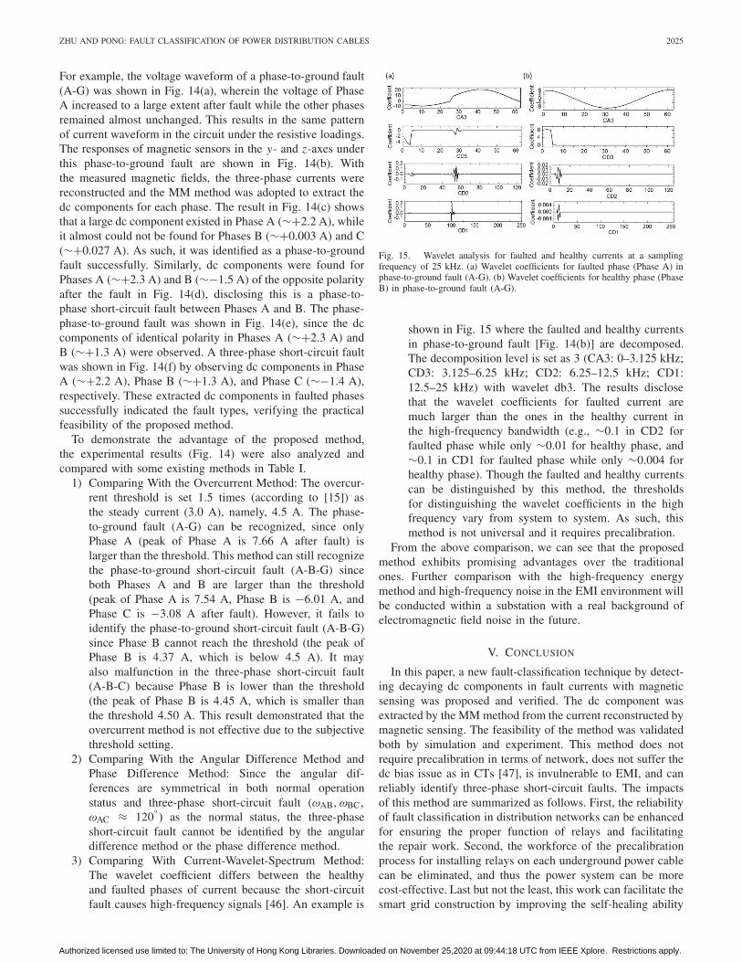
3) Comparing With Current-Wavelet-Spectrum Method:The wavelet coefficient differs between the healthyand faulted phases of current because the short-circuitfault causes high-frequency signals [46]. An example is

Fig. 15. Wavelet analysis for faulted and healthy currents at a samplingfrequency of 25 kHz. (a) Wavelet coefficients for faulted phase (Phase A) inphase-to-ground fault (A-G). (b) Wavelet coefficients for healthy phase (PhaseB) in phase-to-ground fault (A-G).

shown in Fig. 15 where the faulted and healthy currentsin phase-to-ground fault [Fig. 14(b)] are decomposed.The decomposition level is set as 3 (CA3: 0–3.125 kHz;CD3: 3.125–6.25 kHz; CD2: 6.25–12.5 kHz; CD1:12.5–25 kHz) with wavelet db3. The results disclosethat the wavelet coefficients for faulted current aremuch larger than the ones in the healthy current inthe high-frequency bandwidth (e.g., ∼0.1 in CD2 forfaulted phase while only ∼0.01 for healthy phase, and∼0.1 in CD1 for faulted phase while only ∼0.004 forhealthy phase). Though the faulted and healthy currentscan be distinguished by this method, the thresholdsfor distinguishing the wavelet coefficients in the highfrequency vary from system to system. As such, thismethod is not universal and it requires precalibration.

From the above comparison, we can see that the proposedmethod exhibits promising advantages over the traditionalones. Further comparison with the high-frequency energymethod and high-frequency noise in the EMI environment willbe conducted within a substation with a real background ofelectromagnetic field noise in the future.

V. CONCLUSION

In this paper, a new fault-classification technique by detect-ing decaying dc components in fault currents with magneticsensing was proposed and verified. The dc component wasextracted by the MM method from the current reconstructed bymagnetic sensing. The feasibility of the method was validatedboth by simulation and experiment. This method does notrequire precalibration in terms of network, does not suffer thedc bias issue as in CTs [47], is invulnerable to EMI, and canreliably identify three-phase short-circuit faults. The impactsof this method are summarized as follows. First, the reliabilityof fault classification in distribution networks can be enhancedfor ensuring the proper function of relays and facilitatingthe repair work. Second, the workforce of the precalibrationprocess for installing relays on each underground power cablecan be eliminated, and thus the power system can be morecost-effective. Last but not the least, this work can facilitate thesmart grid construction by improving the self-healing ability



in distribution systems and boost the smart city developmentby safeguarding the continuity of power supply [48], [49].

The technique will be tested under different conditions(e.g., different fault times, fault distances, and locations, andnetwork voltage) in a real on-site environment of a powersystem to validate its practical effectiveness in the future work.

REFERENCES

[1] L. S. Czarnecki and Z. Staroszczyk, “On-line measurement of equivalentparameters for harmonic frequencies of a power distribution systemand load,” IEEE Trans. Instrum. Meas., vol. 45, no. 2, pp. 467–472,Apr. 1996.

[2] T. Gönen, Electric Power Distribution System Engineering. New York,NY, USA: McGraw-Hill, 1986.

[3] K. Zhu, W. K. Lee, and P. W. T. Pong, “Non-contact voltage monitoringof HVDC transmission lines based on electromagnetic fields,” IEEESensors J., vol. 19, no. 8, pp. 3121–3129, Apr. 2019.

[4] S. C. Chu, “Screening factor of pipe-type cable systems,” IEEE Trans.Power App. Syst., vol. PAS-88, no. 5, pp. 522–528, May 1969.

[5] O. Quiroga, J. Meléndez, and S. Herraiz, “Fault causes analysis infeeders of power distribution networks,” in Proc. Int. Conf. RenewablesEnergies Qual. Power, 2011, p. 9.

[6] K. Zhu, W. K. Lee, and P. W. T. Pong, “Fault-line identification ofHVDC transmission lines by frequency-spectrum correlation based oncapacitive coupling and magnetic field sensing,” IEEE Trans. Magn.,vol. 54, no. 11, pp. 1–5, Nov. 2018.

[7] P. K. Dash, S. R. Samantaray, and G. Panda, “Fault classification andsection identification of an advanced series-compensated transmissionline using support vector machine,” IEEE Trans. Power Del., vol. 22,no. 1, pp. 67–73, Jan. 2007.

[8] A. de Souza Gomes, M. A. Costa, T. G. A. de Faria, andW. M. Caminhas, “Detection and classification of faults in power trans-mission lines using functional analysis and computational intelligence,”IEEE Trans. Power Del., vol. 28, no. 3, pp. 1402–1413, Jul. 2013.

[9] V. S. Kale, S. R. Bhide, and P. P. Bedekar, “Faulted phase selectionon double circuit transmission line using wavelet transform and neuralnetwork,” in Proc. Int. Conf. Power Syst., Dec. 2009, pp. 1–6.

[10] H. Shu, Q. Wu, X. Wang, and X. Tian, “Fault phase selection anddistance location based on ANN and S-transform for transmission linein triangle network,” in Proc. 3rd Int. Conf. Image Signal Process.,Oct. 2010, pp. 3217–3219.

[11] Z. Q. Bo, R. K. Aggarwal, A. T. Johns, H. Y. Li, and Y. H. Song,“A new approach to phase selection using fault generated high frequencynoise and neural networks,” IEEE Trans. Power Del., vol. 12, no. 1,pp. 106–115, Jan. 1997.

[12] W. M. Al-hassawi, N. H. Abbasi, and M. M. Mansour, “A neural-network-based approach for fault classification and faulted phase selec-tion,” in Proc. Can. Conf. Elect. Comput. Eng., May 1996, pp. 384–387.

[13] P. Gill, Electrical Power Equipment Maintenance and Testing.Boca Raton, FL, USA: CRC Press, 2008.

[14] F. B. Costa, B. A. Souza, and N. S. D. Brito, “A wavelet-based methodfor detection and classification of single and crosscountry faults intransmission lines,” in Proc. Int. Conf. Power Syst. Transients, Jun. 2009,pp. 1–8.

[15] NPTEL. (2019). Overcurrent Protection. Accessed: Mar. 13, 2019.[Online]. Available: https://nptel.ac.in/courses/108101039/download/Lecture-15.pdf

[16] J. Faiz, S. Lotfi-fard, and S. H. Shahri, “Prony-based optimal Bayesfault classification of overcurrent protection,” IEEE Trans. Power Del.,vol. 22, no. 3, pp. 1326–1334, Jul. 2007.

[17] A. Ferrero and G. Superti-Furga, “A new approach to the definitionof power components in three-phase systems under nonsinusoidal con-ditions,” IEEE Trans. Instrum. Meas., vol. 40, no. 3, pp. 568–577,Jun. 1991.

[18] D. Middleton, “Statistical-physical models of electromagnetic inter-ference,” IEEE Trans. Electromagn. Compat., vol. EMC-19, no. 3,pp. 106–127, Aug. 1977.

[19] T. Adu, “An accurate fault classification technique for power sys-tem monitoring devices,” IEEE Trans. Power Del., vol. 17, no. 3,pp. 684–690, Jul. 2002.

[20] C. Zheng et al., “Magnetoresistive sensor development roadmap (non-recording applications),” IEEE Trans. Magn., vol. 55, no. 4, pp. 1–30,Apr. 2019.

[21] Y. S. Cho, C. K. Lee, G. Jang, and H. J. Lee, “An innovative decayingDC component estimation algorithm for digital relaying,” IEEE Trans.Power Del., vol. 24, no. 1, pp. 73–78, Jan. 2009.

[22] J. Machowski, J. Bialek, and J. Bumby, Power System Dynamics:Stability and Control. Hoboken, NJ, USA: Wiley, 2011.

[23] J. Arrillaga and N. R. Watson, Power System Harmonics. Hoboken, NJ,USA:Wiley, 2004.

[24] M. Eremia and M. Shahidehpour, Handbook of Electrical Power SystemDynamics: Modeling, Stability, and Control, vol. 92. Hoboken, NJ, USA:Wiley, 2013.

[25] K. M. Silva, B. A. Souza, and N. S. D. Brito, “Fault detection and clas-sification in transmission lines based on wavelet transform and ANN,”IEEE Trans. Power Del., vol. 21, no. 4, pp. 2058–2063, Oct. 2006.

[26] A. Bernieri, G. Betta, and C. Liguori, “On-line fault detection anddiagnosis obtained by implementing neural algorithms on a digital signalprocessor,” IEEE Trans. Instrum. Meas., vol. 45, no. 5, pp. 894–899,Oct. 1996.

[27] R. Isermann, Fault-Diagnosis Systems: An Introduction From FaultDetection to Fault Tolerance. New York, NY, USA: Springer, 2006.

[28] M. N. Alam, R. H. Bhuiyan, R. A. Dougal, and M. Ali, “Design andapplication of surface wave sensors for nonintrusive power line faultdetection,” IEEE Sensors J., vol. 13, no. 1, pp. 339–347, Jan. 2013.

[29] M. J. Devaney and L. Eren, “Detecting motor bearing faults,” IEEEInstrum. Meas. Mag., vol. 7, no. 4, pp. 30–50, Dec. 2004.

[30] M. Silva, M. Oleskovicz, and D. V. Coury, “A fault locator for trans-mission lines using traveling waves and wavelet transform theory,” inProc. 8th IEE Int. Conf. Develop. Power Syst. Protection, Apr. 2004,pp. 212–215.

[31] P. Dutta, A. Esmaeilian, and M. Kezunovic, “Transmission-line faultanalysis using synchronized sampling,” IEEE Trans. Power Del., vol. 29,no. 2, pp. 942–950, Apr. 2014.

[32] K. Zhu, W. K. Lee, and P. W. T. Pong, “Non-contact capacitive-coupling-based and magnetic-field-sensing-assisted technique for monitoring volt-age of overhead power transmission lines,” IEEE Sensors J., vol. 17,no. 4, pp. 1069–1083, Feb. 2017.

[33] K. Zhu, W. Han, W. K. Lee, and P. W. T. Pong, “On-site non-invasive current monitoring of multi-core underground power cableswith a magnetic-field sensing platform at a substation,” IEEE Sensors J.,vol. 17, no. 6, pp. 1837–1848, Mar. 2017.

[34] A. Canova, F. Freschi, M. Repetto, and M. Tartaglia, “Description ofpower lines by equivalent source system,” Int. J. Comput. Math. Elect.Electron. Eng., vol. 24, no. 3, pp. 893–905, 2005.

[35] L. Davis, Handbook of Genetic Algorithms. Amsterdam,The Netherlands: Elsevier, 1991.

[36] K. Iba, “Reactive power optimization by genetic algorithm,” IEEE Trans.Power Syst., vol. 9, no. 2, pp. 685–692, May 1994.

[37] J. Buse, D. Y. Shi, T. Y. Ji, and Q. H. Wu, “Decaying DC offset removaloperator using mathematical morphology for phasor measurement,” inProc. IEEE PES Innov. Smart Grid Technol. Conf. Eur., Oct. 2010,pp. 1–6.

[38] J. Serra, “Introduction to mathematical morphology,” Comput. Vis.,Graph., Image Process., vol. 35, pp. 283–305, Sep. 1986.

[39] P. Duhamel and M. Vetterli, “Fast Fourier transforms: A tutorial reviewand a state of the art,” Signal Process., vol. 19, no. 4, pp. 259–299,1990.

[40] A. A. bin M. Zin, J. Tavalaei, and M. H. bin Habibuddin, “Sim-ulation of distance relay operation on fault condition in MATLABsoftware/simulink,” Proc. Elect. Eng. Comput. Sci. Inform., vol. 1, no. 1,pp. 355–360, 2014.

[41] J. Park, A. John Park, and S. Mackay, Practical Data Acquisition forInstrumentation and Control Systems. Boston, MA, USA: Newnes, 2003.

[42] K. J. O’Donovan, R. Kamnik, D. T. O’Keeffe, and G. M. Lyons,“An inertial and magnetic sensor based technique for joint angle mea-surement,” J. Biomech., vol. 40, no. 12, pp. 2604–2611, 2007.

[43] Honeywell. (2011). 3-Axis Magnetic Sensor Hybrid HMC2003.Accessed: 19. Jul, 2018 [Online]. Available: https://neurophysics.ucsd.edu/Manuals/Honeywell/HMC_2003.pdf

[44] K. Zhu, X. Liu, and P. W. T. Pong, “On-site real-time current monitor-ing of three-phase three-core power distribution cables with magneticsensing,” in Proc. IEEE Sensors, Oct. 2018, pp. 1–4.

[45] Honeywell. (2018). SET/RESET Pulse Circuits for Magnetic Sen-sors. Accessed: 19. Jul, 2018. [Online]. Available: https://neurophysics.ucsd.edu/Manuals/Honeywell/AN-201.pdf

[46] A. W. Galli and O. M. Nielsen, “Wavelet analysis for power systemtransients,” IEEE Comput. Appl. Power, vol. 12, no. 1, pp. 16–25,Jan. 1999.



[47] M. S. Ballal, M. G. Wath, and H. M. Suryawanshi, “A novel approachfor the error correction of CT in the presence of harmonic distortion,”IEEE Trans. Instrum. Meas., to be published.

[48] X. Liu et al., “Overview of Spintronic sensors, Internet of things,and smart living,” 2016, arXiv:1611.00317. [Online]. Available:https://arxiv.org/abs/1611.00317

[49] A. Cocchia, “Smart and digital city: A systematic literature review,” inSmart City. New York, NY, USA: Springer, 2014, pp. 13–43.

Ke Zhu was born in Yichang, China, in 1990. Hereceived the B.Eng. degree in electrical engineer-ing from China Three Gorges University (CTGU),Yichang, in 2013, the Ph.D. degree in electricaland electronic engineering from the University ofHong Kong (HKU), Hong Kong, in 2018.

He is currently a Post-Doctoral Researcher withHKU. His current research interests include com-putational electromagnetics, electric power transmis-sion monitoring, and application of magnetoresistive(MR) sensors in the smart grid.

Dr. Zhu is a member of the IEEE Magnetics Society (Hong Kong Chapter).

Philip W. T. Pong received the B.Eng. degree(First Class Hons.) in electrical and electronicengineering from the University of Hong Kong(HKU), Hong Kong, in 2002, and the Ph.D. degreein engineering from the University of Cambridge,Cambridge, U.K., in 2005.

He was a Post-Doctoral Researcher at the Mag-netic Materials Group, National Institute of Stan-dards and Technology (NIST), Gaithersburg, MD,USA. In 2008, he joined the Department of Elec-trical and Electronic Engineering, HKU, where he

is currently an Associate Professor and involved in the development ofmagnetoresistive (MR) sensors, and the applications of MR sensors in smartgrid and smart living.

Dr. Pong serves as a fellow of the Institution of Engineering and Technology,the Institute of Materials, Minerals and Mining, and the NANOSMAT Society,and a corporate member of Hong Kong Institution of Engineers (HKIE)in Electrical Division, Electronics Division and Energy Division. He was arecipient of the HKIE Young Engineer of the Year Award in 2016. He isserving on the Administrative Committee of the IEEE Magnetics Society.He is a Chartered Physicist, a Chartered Energy Engineer, and a RegisteredProfessional Engineer. He serves as an Editorial Board Member for three SCIjournals.


Documents

Fault Classification of Power Distribution Cables by