Fault Detection in State Variable Filter Circuit Using ... papers/MIDEM_46(2016)4p209.pdf · Fault Detection in State Variable Filter Circuit Using Kernel Extreme Learning Machine

209

Original scientific paper

MIDEM Society

Fault Detection in State Variable Filter Circuit Using Kernel Extreme Learning Machine (KELM) AlgorithmM. Shanthi1, M. C. Bhuvaneswari2

1Associate Professor Department of Electronics and Communication Engineering, Kumaraguru College of Technology, Tamil Nadu, India2Associate Professor Department of Electrical and Electronics Engineering, Tamil Nadu, India

Abstract: Electronic applications have become important in industry, science, and everyday life. Modern applications demand greater complexity and smaller packaging, which makes testing more critical. Testing of analog circuit contributes major cost in IC manufacturing. This paper proposes a new method for fault classification in analog circuits using Extreme Learning Machine (ELM) and Kernel ELM algorithms.ELM is a single hidden layer feed forward neural network (SLFN) which chooses the input weight randomly and computes the output weight analytically. The features of the benchmark circuit are extracted by simulating the transfer function of the circuit. The fault dictionary constructed from the features of the circuit is used as the inputs to the ELM and KELM algorithm. Simulation results show that KELM algorithm has better performance at faster learning speed than the ELM algorithm. KELM algorithm outperforms BP-NN-based and ELM-based approaches significantly with effective classification.

Keywords: Analog circuits; Neural network; fault detection; Extreme learning machine

Iskanje napak v filtru na osnovi spremenljivk stanja z algoritmom ekstremnega strojnega učenja na osnovi jedrne funkcije (KELM)Izvleček: Elektronske naprave so postale pomembne tako v industriji kot v vsakdanjem življenju. Moderne naprave zahtevajo večjo kompleksnost in manjše ohišje, kar otežuje njihovo testiranje. Testiranje analognih vezij predstavlja največji strošek proizvajalcev integriranih vezij. Članek predlaga novo metodo klasifikacije napak v analognih vezjih s pomočjo ekstremnega strojnega učenja (ELM) in ELM algoritma na osnovi jedrne funkcije. ELM je skrita enonivojska naprej usmerjena nevronska mreža (SLFN), ki vhodno utež izbere naključno in analitično izračuna izhodno utež. Lastnosti ocenjevalnega vezja so izluščeni s pomočjo simulacij prenosne funkcije vezja. Nabor napak na osnovi lastnosti vezja predstavlja vhod ELM in KELM algoritmu. Simulacije nakazujejo, da ima KELM algoritem boljše lastnosti in izkazuje hitrejše učenje kot ELM algoritem. KELM algoritem močno presega BP-NN in ELM pristope z učinkovito klasifikacijo.

Ključne besede: Analogna vezja; nevronske mreže; odkrivanje napak; ekstremno strojno učenje

* Corresponding Author’s e-mail: [email protected]

Journal of Microelectronics, Electronic Components and MaterialsVol. 46, No. 4(2016), 209 – 218

1 Introduction

The System-on-chip (SOC) technology has raised the importance of analog circuitry, moving it more into mainstream integrated circuit (IC) design. The advance-ments in IC technology and co-existence of analog and digital signals make testing, a challenging task. There-fore, electronic tests are system dependent and there

are different fault diagnosis methods based on the signal nature[1].There are very limited number of test-ing tools available for analog and mixed signal circuits. Analog and mixed signal IC’s have complex functions in which traditional functional testing methods cannot be applied. Analog fault diagnosis is complex and chal-lenging because of the absence of efficient fault mod-

210

els, component tolerance, and non-linearity [2]. The fault diagnosis of analog circuits is generally classified into Simulation After Test (SAT) and Simulation Before Test (SBT). SBT is suitable for recent research work and is the most preferred [3]. Fault in analog circuits is clas-sified into hard faults and soft faults. Among the vari-ous approaches, the approximation methodology can be used for modeling the dynamic system and its fail-ure. Some important approximation models are spline, radial bias function, Artificial Neural Network (ANN), and adaptive fuzzy system. ANN has gained more im-portance recently in soft fault diagnosis as it has high learning capability [4].

Analog testing includes two parts: Test pattern genera-tion and fault diagnosis. There are many researches in both the parts of the analog testing Pan and Cheng (1999) proposed a novel and cost effective technique for Linear Time Invariant (LTI) analog circuits by deriv-ing hyperplanes in the multidimensional space formed by CUT’s parameters. This method has superior classifi-cation performance, but has an inadequate testing ac-curacy [5]. Test generation algorithm based on Support Vector Machine (SVM) is proposed by Long et.al which is used for classification [6]. Balivada et.al method of test generation is based on deriving amplitude and phase error from the steady state sinusoidal waveform which is used for fault detection [7]. Hamida et.al pro-posed and developed software for sensitive testing and generation of test patterns for soft and hard faults [8]. Devanarayanadurg and Soma developed a dynamic programming method based on minmax formulation which is used to construct, test waveforms for on-chip test scheme and this method requires high time cost for large circuits [9]. Long et al proposed a Simulation Before Test (SBT) based method on analog circuits in 2011[10].Yang et.al proposed a method based on the heuristic graph selection approach for the selection of test points to construct fault dictionary [11].Yang et al proposed a continuous fault model using the com-ponent connection model (CCM). CCM can find fault location, but the size of CCM increases as the circuit becomes complex [12]. Li and Xie proposed a fault di-agnosis method based on Kalman filter. This method is used for diagnosing both parametric and catastrophic faults [13].

Nowadays fault diagnosis based on the machine learn-ing is used for analog circuits. Support Vector Machines (SVM) are widely used as a fault classifier in analog cir-cuits [14-20]. The SVM algorithm maps the lower-di-mensional non-linear space into high dimensional fea-ture space for effective classification and provides high accuracy. However, this algorithm involves higher com-plex computation and time consumption. To solve the

above problems, a new fault detection model based on machine learning called Extreme Learning Machine (ELM) [21-25] with lower time consumption and simple process has been proposed in this paper. The accuracy of classification is not sensitive to trade-off parameters and so has good classification performance without optimization of trade-off parameters in compressing the sampled space. ELM provides better generalization performance at a faster learning speed with less hu-man intervention.

The main contributions of this paper are summarized as follows:(1) The Kernel ELM classifier is proposed to detect

faults in analog circuit in an efficient and effective way.

(2) The proposed diagnostic system has achieved excellent classification results compared with the existing methods in previous studies.

The organization of the paper is as follows. Section 2 deals with a brief review of the system description. Section 3 provides a basic description of ELM method. Section 4 describes the Kernel based ELM algorithm and the fault classification by ELM and KELM algorithm. Section 5 discusses simulation results. Section 6 pre-sents the conclusion of the paper.

2 System description

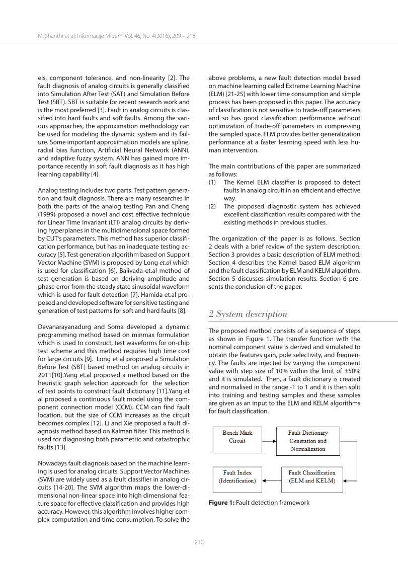
The proposed method consists of a sequence of steps as shown in Figure 1. The transfer function with the nominal component value is derived and simulated to obtain the features gain, pole selectivity, and frequen-cy. The faults are injected by varying the component value with step size of 10% within the limit of ±50% and it is simulated. Then, a fault dictionary is created and normalised in the range -1 to 1 and it is then split into training and testing samples and these samples are given as an input to the ELM and KELM algorithms for fault classification.

Figure 1: Fault detection framework

M. Shanthi et al; Informacije Midem, Vol. 46, No. 4(2016), 209 – 218

211

2.1 State Variable Filter

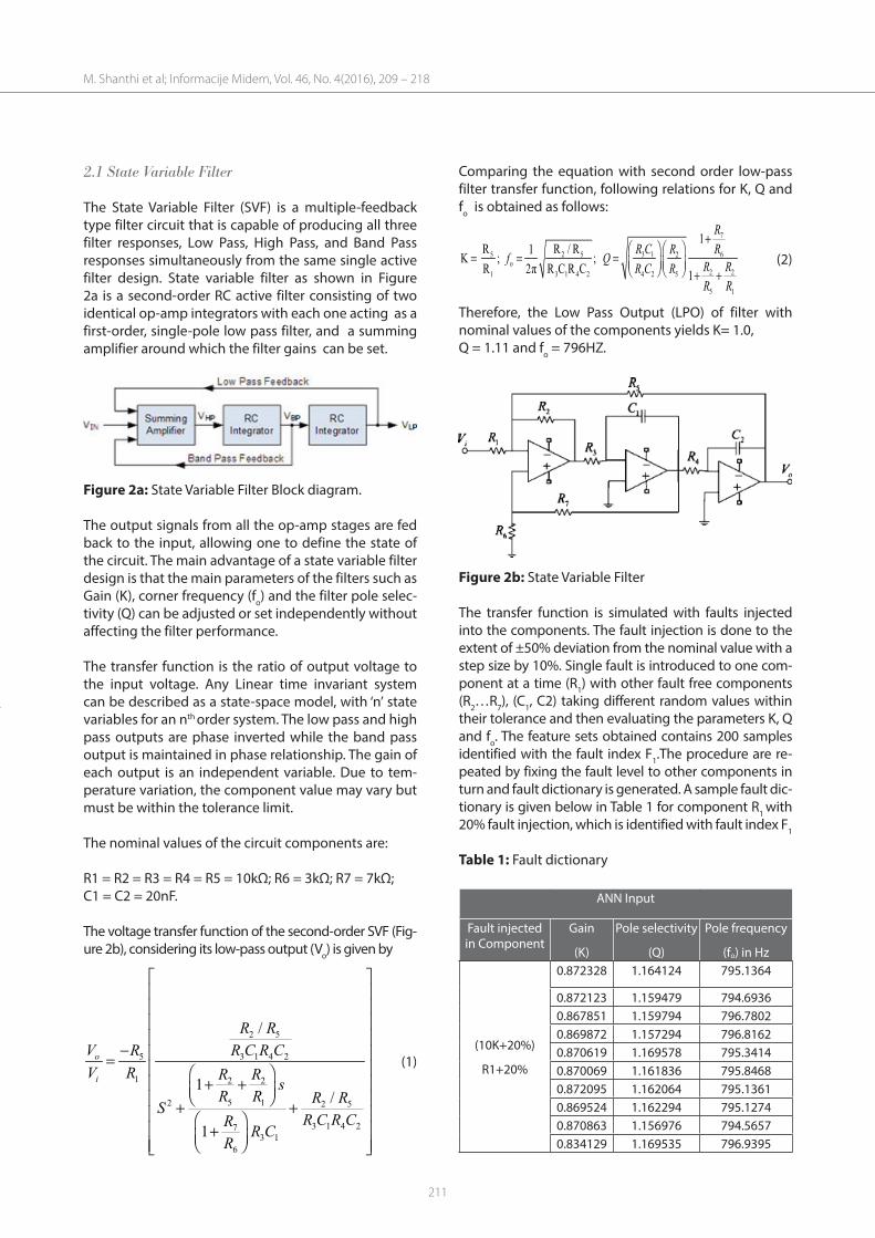
The State Variable Filter (SVF) is a multiple-feedback type filter circuit that is capable of producing all three filter responses, Low Pass, High Pass, and Band Pass responses simultaneously from the same single active filter design. State variable filter as shown in Figure 2a is a second-order RC active filter consisting of two identical op-amp integrators with each one acting as a first-order, single-pole low pass filter, and a summing amplifier around which the filter gains can be set.

Figure 2a: State Variable Filter Block diagram.

The output signals from all the op-amp stages are fed back to the input, allowing one to define the state of the circuit. The main advantage of a state variable filter design is that the main parameters of the filters such as Gain (K), corner frequency (fo) and the filter pole selec-tivity (Q) can be adjusted or set independently without affecting the filter performance.

The transfer function is the ratio of output voltage to the input voltage. Any Linear time invariant system can be described as a state-space model, with ‘n’ state variables for an nth order system. The low pass and high pass outputs are phase inverted while the band pass output is maintained in phase relationship. The gain of each output is an independent variable. Due to tem-perature variation, the component value may vary but must be within the tolerance limit.

The nominal values of the circuit components are:

R1 = R2 = R3 = R4 = R5 = 10kΩ; R6 = 3kΩ; R7 = 7kΩ; C1 = C2 = 20nF.

The voltage transfer function of the second-order SVF (Fig-ure 2b), considering its low-pass output (Vo) is given by

2 5

5 3 1 4 2

1 2 2

5 12 2 5

3 1 4 273 1

6

/

1/

1

o

i

R RV R R C R CV R R R s

R R R RSR C R CR R C

R

− = + + + + +

(1)

Comparing the equation with second order low-pass filter transfer function, following relations for K, Q and fo is obtained as follows: 7

5 2 5 3 1 62o

2 21 3 1 4 2 4 2 5

5 1

1R R / R1K ; ; R 2π R C R C 1

RR C RRf Q R RR C R

R R

+

= = = + + (2)

Therefore, the Low Pass Output (LPO) of filter with nominal values of the components yields K= 1.0, Q = 1.11 and fo = 796HZ.

Figure 2b: State Variable Filter

The transfer function is simulated with faults injected into the components. The fault injection is done to the extent of ±50% deviation from the nominal value with a step size by 10%. Single fault is introduced to one com-ponent at a time (R1) with other fault free components (R2…R7), (C1, C2) taking different random values within their tolerance and then evaluating the parameters K, Q and fo. The feature sets obtained contains 200 samples identified with the fault index F1.The procedure are re-peated by fixing the fault level to other components in turn and fault dictionary is generated. A sample fault dic-tionary is given below in Table 1 for component R1 with 20% fault injection, which is identified with fault index F1

Table 1: Fault dictionary

ANN Input

Fault injected in Component

Gain

(K)

Pole selectivity

(Q)

Pole frequency

(fo) in Hz

(10K+20%)

R1+20%

0.872328 1.164124 795.1364

0.872123 1.159479 794.69360.867851 1.159794 796.78020.869872 1.157294 796.81620.870619 1.169578 795.34140.870069 1.161836 795.84680.872095 1.162064 795.13610.869524 1.162294 795.12740.870863 1.156976 794.56570.834129 1.169535 796.9395


212

There are totally nine components in the circuit, so that the total fault index is nine for a single fault. The features correspond to component values, gain, pole selectivity, and frequency. The data set obtained con-tains 1403 samples for training and 450 samples for testing with four features and nine fault indexes for nine components. The fault dictionary sample for R1+20% includes features of gain, pole selectivity and pole frequency and their corresponding sample values are 0.872328, 1.159479 and 794.6936 respectively. A similar procedure is followed to all the components for assigning fault index corresponding to the faulty com-ponent and creating a fault dictionary.

3 Extreme Learning Machine (ELM)

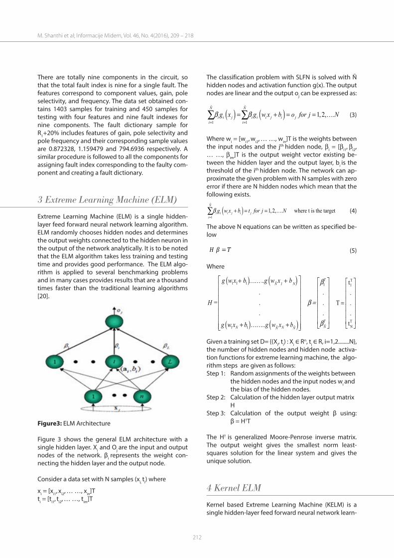
Extreme Learning Machine (ELM) is a single hidden-layer feed forward neural network learning algorithm. ELM randomly chooses hidden nodes and determines the output weights connected to the hidden neuron in the output of the network analytically. It is to be noted that the ELM algorithm takes less training and testing time and provides good performance. The ELM algo-rithm is applied to several benchmarking problems and in many cases provides results that are a thousand times faster than the traditional learning algorithms [20].

Figure3: ELM Architecture

Figure 3 shows the general ELM architecture with a single hidden layer. Xi and Oj are the input and output nodes of the network. βi represents the weight con-necting the hidden layer and the output node.

Consider a data set with N samples (xi, ti) where

xi = [xi1, xi2, … …, xin]Tti = [ti1, ti2, … …, tim]T

The classification problem with SLFN is solved with Ñ hidden nodes and activation function g(x). The output nodes are linear and the output oj can be expressed as:

( ) ( )

1 1 1, 2, .

N N

i i j i i i j i ji i

g x g w x b o for j Nβ β= =

= + = = …∑ ∑

(3)

Where wi = [wi1, wi2, … …, win]T is the weights between the input nodes and the jth hidden node, bi = [bi1, bi2, … …, bim]T is the output weight vector existing be-tween the hidden layer and the output layer, bi is the threshold of the ith hidden node. The network can ap-proximate the given problem with N samples with zero error if there are N hidden nodes which mean that the following exists.

( )1

1, 2, . where t is the target N

i i i j i ji

g w x b t for j Nβ=

+ = = …∑

(4)

The above N equations can be written as specified be-low

= (5)

Where

( ) ( )

( ) ( )

1 1 1 1

1 1

... .

. .. .

..

TN 1 N

TNN NN N

g w x b g w x b

H =

g w x b g w x b

β

β =

β

+ …… +

+ …… +

T1

TN

t.

T ..

t

=

Given a training set D= (Xi, ti) : Xi ∈ Rn, ti ∈ R, i=1,2........N, the number of hidden nodes and hidden node activa-tion functions for extreme learning machine, the algo-rithm steps are given as follows:Step 1: Random assignments of the weights between the hidden nodes and the input nodes wi and the bias of the hidden nodes. Step 2: Calculation of the hidden layer output matrix

H Step 3: Calculation of the output weight β using:

β = H†T

The H† is generalized Moore-Penrose inverse matrix. The output weight gives the smallest norm least-squares solution for the linear system and gives the unique solution.

4 Kernel ELM

Kernel based Extreme Learning Machine (KELM) is a single hidden-layer feed forward neural network learn-


213

ing algorithm. In KELM, the numbers of hidden nodes are not chosen; it is arbitrarily determined by the al-gorithm based on the application. The ELM algorithm determines the initial parameters of input weights and biases randomly with simple kernel function. The stability and generalization performance of the KELM algorithm is determined by these input parameters. KELM improves the stability and performance by elimi-nating feature mapping of hidden neurons and with the group of activation functions. KELM has kernel parameters which are optimized to improve the gen-eralization performance. KELM is used to overcome the drawbacks of ELM algorithm.

The KELM algorithm with fast learning speed and good generalization performance is widely used in many fields. In KELM, the initial parameters of the hidden lay-er need not be tuned and all nonlinear piecewise con-tinuous functions can be used as the hidden neurons. Considering the N arbitrary distinct samples (xi, ti) | xi ∈ Rn, ti ∈ Rm, i=1,2,......,N the output function in KELM with L hidden neurons is

( ) ( ) ( )1

L

L i ii

f x h x h xβ β=

= =∑ (6)

β= [β1, β2,......, βL] is the vector of output weights be-tween the hidden layer of L neurons and the output neuron and h(x) =[ h1(x),h2(x),......, hL(x)] is the output vector of the hidden layer with respect to the input x and it maps the data from input space to the ELM’s fea-ture space.

In order to improvise the generalization performance and to decrease the training error the output weight and training error should be minimized at the same time.

Minimize Hβ T , β− (7)

Where ||Hβ-T|| is the training error and ||β|| is the output weight.

The least square solution based on Karush-Kuhn-Tuker theorems (KKT) conditions the output weight β which can be written as

11T TH HH TC

− β = +

(8)

where H is the hidden layer output matrix, C is the regularization coefficient and T is the expected output matrix of the input samples.

The output function of the KELM learning algorithm is

( ) ( )

11T Tf x h x H HH TC

− = +

(9)

If the feature mapping of h(x) is unknown and the ker-nel matrix based on Mercer’s conditions is defined as

( ) ( ) ( ): , Tij i j i jM HH m h x h x k x x= = = (10)

The output function of KELM can be defined as

( ) ( ) ( )1

11 [ , , , , ] Nf x k x x k x x M TC

− = …… +

(11)

Where M=HHT and k(x, y) is the kernel function of the hidden neurons of a single hidden layer feed-forward neural networks.

There are many kernel functions such as linear kernel, polynomial kernel, Gaussian kernel, and exponential kernel which satisfy the Mercer condition available from the existing literature. It is observed that different types of kernel activation functions have great influ-ence on the performance of KELM. In this kernel-based ELM, the hidden layer feature mapping ℎ (𝑥) need not to be known to the user. In addition, the number of hid-den nodes 𝐿 need not be specified.

RBF kernels can be randomly generated instead of be-ing tuned. This allows the centers and impact widths of RBF kernels to randomly generate and analytically calculate the output weights instead of iterative tun-ing. The kernel function of ELM can be any nonlinear bounded integral function which is almost continuous anywhere.

4.1 Fault detection and classification using ELM and KELM

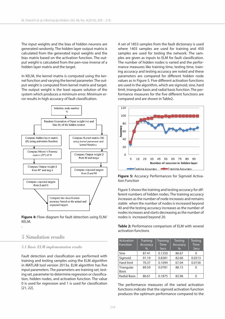
The flow diagram of the proposed ELM and KELM al-gorithm is shown in Figure 4.The training and testing samples are obtained from the fault dictionary. Sev-enty five percentages of data are chosen for training and twenty five percentages of data is chosen for test-ing. The testing and training data are chosen randomly and are normalized in the range -1 to 1.The normalized training and testing data are given as an input to the al-gorithm. As described earlier, the four dimensional fea-ture vectors consisting of component value, gain, pole selectivity, and frequency are taken as an input for ELM to classify faults. Twenty hidden nodes with various ac-tivation functions are used for the ELM. ELM has five input parameters such as training data, testing data, number of hidden nodes, activation function and a pa-rameter to determine regression or classification. The output of the algorithm implementation is the correct detection of the fault index as per the target defined.


214

The input weights and the bias of hidden neurons are generated randomly. The hidden layer output matrix is calculated from the generated input weights and the bias matrix based on the activation function. The out-put weight is calculated from the pen-rose inverse of a hidden layer matrix and the target.

In KELM, the kernel matrix is computed using the ker-nel function and varying the kernel parameter. The out-put weight is computed from kernel matrix and target. The output weight is the least square solution of the system which produces a minimum error. Minimum er-ror results in high accuracy of fault classification.

Figure 4: Flow diagram for fault detection using ELM/KELM. .

5 Simulation results

5.1 Basic ELM implementation results

Fault detection and classification are performed with training and testing samples using the ELM algorithm in MATLAB tool version 2013a. ELM algorithm has five input parameters. The parameters are training set, test-ing set, parameter to determine regression or classifica-tion, hidden nodes, and activation function. The value 0 is used for regression and 1 is used for classification [21, 22].

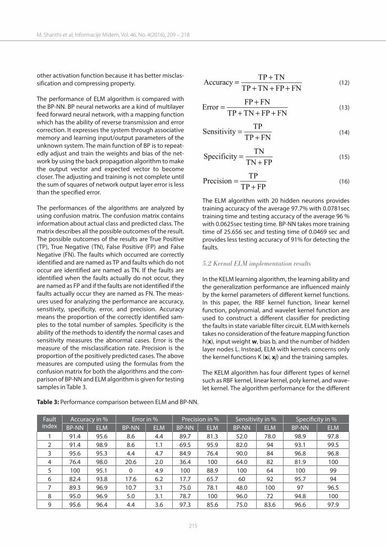
A set of 1853 samples from the fault dictionary is used where 1403 samples are used for training and 450 samples are used for testing the network. The sam-ples are given as inputs to ELM for fault classification. The number of hidden nodes is varied and the perfor-mance measures like training time, testing time, train-ing accuracy and testing accuracy are noted and these parameters are compared for different hidden node values as in Figure 5. Five different activation functions are used in the algorithm, which are sigmoid, sine, hard limit, triangular basis and radial basis function. The per-formance measures for the five different functions are compared and are shown in Table2.

Figure 5: Accuracy Performances for Sigmoid Activa-tion Function

Figure 5 shows the training and testing accuracy for dif-ferent numbers of hidden nodes. The training accuracy increases as the number of node increases and remains stable when the number of nodes is increased beyond 40 and the testing accuracy increases as the number of nodes increases and starts decreasing as the number of nodes is increased beyond 20.

Table 2: Performance comparison of ELM with several activation functions

Activation Function

Training Accuracy

%

Training TimeSecs

Testing Accuracy

%

Testing Time Secs

Sine 87.41 0.1250 86.67 0Sigmoid 91.19 0.8281 82.66 0.0313Hard limit 70.37 0.1094 67.04 0.0156Triangular Basis

89.59 0.0781 88.15 0

Radial Basis 86.61 0.1875 82.96 0

The performance measures of the varied activation functions indicate that the sigmoid activation function produces the optimum performance compared to the


215

other activation function because it has better misclas-sification and compressing property. The performance of ELM algorithm is compared with the BP-NN. BP neural networks are a kind of multilayer feed forward neural network, with a mapping function which has the ability of reverse transmission and error correction. It expresses the system through associative memory and learning input/output parameters of the unknown system. The main function of BP is to repeat-edly adjust and train the weights and bias of the net-work by using the back propagation algorithm to make the output vector and expected vector to become closer. The adjusting and training is not complete until the sum of squares of network output layer error is less than the specified error.

The performances of the algorithms are analyzed by using confusion matrix. The confusion matrix contains information about actual class and predicted class. The matrix describes all the possible outcomes of the result. The possible outcomes of the results are True Positive (TP), True Negative (TN), False Positive (FP) and False Negative (FN). The faults which occurred are correctly identified and are named as TP and faults which do not occur are identified are named as TN. If the faults are identified when the faults actually do not occur, they are named as FP and if the faults are not identified if the faults actually occur they are named as FN. The meas-ures used for analyzing the performance are accuracy, sensitivity, specificity, error, and precision. Accuracy means the proportion of the correctly identified sam-ples to the total number of samples. Specificity is the ability of the methods to identify the normal cases and sensitivity measures the abnormal cases. Error is the measure of the misclassification rate. Precision is the proportion of the positively predicted cases. The above measures are computed using the formulas from the confusion matrix for both the algorithms and the com-parison of BP-NN and ELM algorithm is given for testing samples in Table 3.

TP TNAccuracy TP TN FP FN

+=+ + +

(12)

FP FN Error TP TN FP FN

+=+ + +

(13)

TP Sensitivity TP FN

=+

(14)

TN Specificity TN FP

=+

(15)

TP Precision TP FP

=+

(16)

The ELM algorithm with 20 hidden neurons provides training accuracy of the average 97.7% with 0.0781sec training time and testing accuracy of the average 96 % with 0.0625sec testing time. BP-NN takes more training time of 25.656 sec and testing time of 0.0469 sec and provides less testing accuracy of 91% for detecting the faults.

5.2 Kernal ELM implementation results

In the KELM learning algorithm, the learning ability and the generalization performance are influenced mainly by the kernel parameters of different kernel functions. In this paper, the RBF kernel function, linear kernel function, polynomial, and wavelet kernel function are used to construct a different classifier for predicting the faults in state variable filter circuit. ELM with kernels takes no consideration of the feature mapping function h(x), input weight w, bias b, and the number of hidden layer nodes L. Instead, ELM with kernels concerns only the kernel functions K (xi, xj) and the training samples.

The KELM algorithm has four different types of kernel such as RBF kernel, linear kernel, poly kernel, and wave-let kernel. The algorithm performance for the different

Table 3: Performance comparison between ELM and BP-NN.

Fault index

Accuracy in % Error in % Precision in % Sensitivity in % Specificity in %BP-NN ELM BP-NN ELM BP-NN ELM BP-NN ELM BP-NN ELM

1 91.4 95.6 8.6 4.4 89.7 81.3 52.0 78.0 98.9 97.82 91.4 98.9 8.6 1.1 69.5 95.9 82.0 94 93.1 99.53 95.6 95.3 4.4 4.7 84.9 76.4 90.0 84 96.8 96.84 76.4 98.0 20.6 2.0 36.4 100 64.0 82 81.9 1005 100 95.1 0 4.9 100 88.9 100 64 100 996 82.4 93.8 17.6 6.2 17.7 65.7 60 92 95.7 947 89.3 96.9 10.7 3.1 75.0 78.1 48.0 100 97 96.58 95.0 96.9 5.0 3.1 78.7 100 96.0 72 94.8 1009 95.6 96.4 4.4 3.6 97.3 85.6 75.0 83.6 96.6 97.9


216

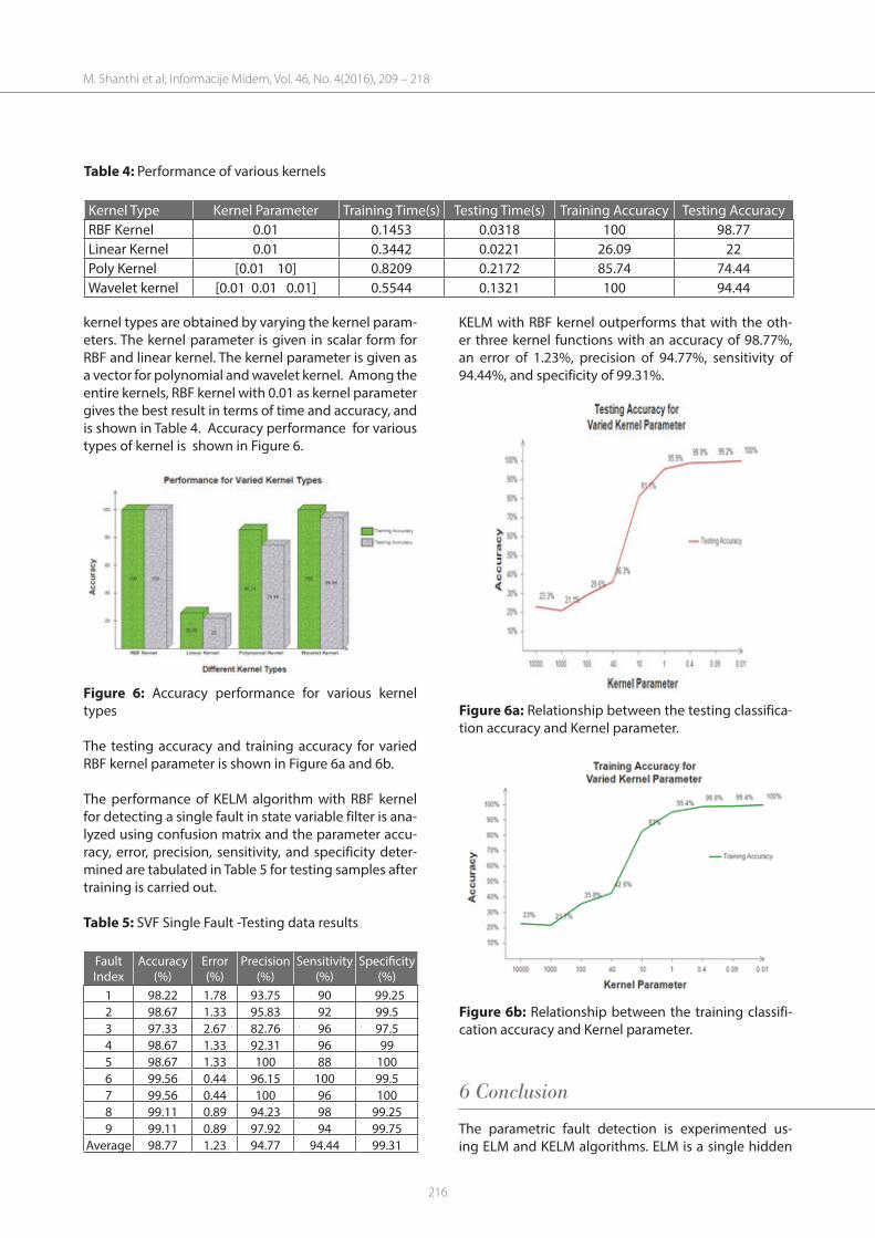
kernel types are obtained by varying the kernel param-eters. The kernel parameter is given in scalar form for RBF and linear kernel. The kernel parameter is given as a vector for polynomial and wavelet kernel. Among the entire kernels, RBF kernel with 0.01 as kernel parameter gives the best result in terms of time and accuracy, and is shown in Table 4. Accuracy performance for various types of kernel is shown in Figure 6.

Figure 6: Accuracy performance for various kernel types

The testing accuracy and training accuracy for varied RBF kernel parameter is shown in Figure 6a and 6b. The performance of KELM algorithm with RBF kernel for detecting a single fault in state variable filter is ana-lyzed using confusion matrix and the parameter accu-racy, error, precision, sensitivity, and specificity deter-mined are tabulated in Table 5 for testing samples after training is carried out.

Table 5: SVF Single Fault -Testing data results

Fault Index

Accuracy (%)

Error (%)

Precision (%)

Sensitivity (%)

Specificity (%)

1 98.22 1.78 93.75 90 99.252 98.67 1.33 95.83 92 99.53 97.33 2.67 82.76 96 97.54 98.67 1.33 92.31 96 995 98.67 1.33 100 88 1006 99.56 0.44 96.15 100 99.57 99.56 0.44 100 96 1008 99.11 0.89 94.23 98 99.259 99.11 0.89 97.92 94 99.75

Average 98.77 1.23 94.77 94.44 99.31

KELM with RBF kernel outperforms that with the oth-er three kernel functions with an accuracy of 98.77%, an error of 1.23%, precision of 94.77%, sensitivity of 94.44%, and specificity of 99.31%.

Table 4: Performance of various kernels

Kernel Type Kernel Parameter Training Time(s) Testing Time(s) Training Accuracy Testing AccuracyRBF Kernel 0.01 0.1453 0.0318 100 98.77Linear Kernel 0.01 0.3442 0.0221 26.09 22Poly Kernel [0.01 10] 0.8209 0.2172 85.74 74.44Wavelet kernel [0.01 0.01 0.01] 0.5544 0.1321 100 94.44

Figure 6b: Relationship between the training classifi-cation accuracy and Kernel parameter.

Figure 6a: Relationship between the testing classifica-tion accuracy and Kernel parameter.


6 Conclusion

The parametric fault detection is experimented us-ing ELM and KELM algorithms. ELM is a single hidden

217

layer feed forward neural network (SLFN) and itera-tive tuning is not needed for the hidden layer. The al-gorithm randomly chooses the input weight and the bias matrix. The hidden layer output is calculated from the activation function and the randomly generated input matrices. The hidden layer output is used in the computation of the output weight which is used in the calculation of training and testing accuracy. The com-parison shows that the sigmoid activation function and twenty hidden neurons of ELM algorithm provides 97.7% training accuracy with 0.0781sec training time and testing accuracy of 96% with a 0.0625 sec testing time. This algorithm saves time efficiently. The result is compared with the BP–NN single layer architecture with the same twenty neurons for the same state vari-able filter. The training time obtained is 25.656 seconds and the testing time of 0.0469 seconds with testing ac-curacy of 91%.The results indicate that ELM provides better scalability and generalization performance at faster learning speed. The comparison between ELM and KELM is carried out which shows that KELM pro-vides 100% training accuracy and 98.77% testing ac-curacy with RBF kernel. The results indicate that KELM achieves higher accuracy performance.

7 References

1. Zhou, J., Tian, S., Yang, C., & Ren, X. (2014). Test gen-eration algorithm for fault detection of analog cir-cuits based on extreme learning machine. Com-putational intelligence and neuroscience, 2014, 55.

2. Nagi, N., & Abraham, J. A. (1992, April). Hierarchi-cal fault modeling for analog and mixed-signal circuits. In VLSI Test Symposium, 1992.’10th An-niversary. Design, Test and Application: ASICs and Systems-on-a-Chip’, Digest of Papers, 1992 IEEE (pp. 96-101). IEEE.

3. Bandler, J. W., & Salama, A. E. (1985). Fault diagno-sis of analog circuits. Proceedings of the IEEE, 73(8), 1279-1325.

4. Yuan, L., He, Y., Huang, J., & Sun, Y. (2010). A new neural-network-based fault diagnosis approach for analog circuits by using kurtosis and entropy as a preprocessor. IEEE Transactions on Instrumen-tation and Measurement, 59(3), 586-595.

5. Pan, C. Y., & Cheng, K. T. (1999). Test generation for linear time-invariant analog circuits. IEEE Transac-tions on Circuits and Systems II: Analog and Digital Signal Processing, 46(5), 554-564.

6. Long, T., Wang, H., & Long, B. (2011). Test genera-tion algorithm for analog systems based on sup-port vector machine. Signal, Image and Video Pro-cessing, 5(4), 527-533.

7. Balivada, A., Chen, J., & Abraham, J. A. (1996). Analog testing with time response parameters. IEEE Design & Test, 13(2), 18-25.

8. Hamida, N. B., Saab, K., Marche, D., Kaminska, B., & Quesnel, G. (1996, October). LIMSoft: Automated tool for design and test integration of analog cir-cuits. In Test Conference, 1996. Proceedings. Inter-national (pp. 571-580). IEEE.

9. Devarayanadurg, G., & Soma, M. (1995, Novem-ber). Dynamic test signal design for analog ICs. In Computer-Aided Design, 1995. ICCAD-95. Digest of Technical Papers. 1995 IEEE/ACM International Con-ference on (pp. 627-630). IEEE.

10. Long, T., Wang, H., & Long, B. (2011). A classical pa-rameter identification method and a modern test generation algorithm. Circuits, Systems, and Signal Processing, 30(2), 391-412.

11. Yang, C., Tian, S., & Long, B. (2009). Application of heuristic graph search to test-point selection for analog fault dictionary techniques. IEEE Transac-tions on Instrumentation and Measurement, 58(7), 2145-2158.

12. Yang, C., Tian, S., & Long, B. (2009). Test points selection for analog fault dictionary techniques. Journal of Electronic Testing, 25(2-3), 157-168.

13. Li, X., Xie, Y., Bi, D., & Ao, Y. (2013). Kalman filter based method for fault diagnosis of analog cir-cuits. Metrology and Measurement Systems, 20(2), 307-322.

14. Long, B., Tian, S., & Wang, H. (2012). Diagnostics of filtered analog circuits with tolerance based on LS-SVM using frequency features. Journal of Elec-tronic Testing, 28(3), 291-300.

15. Long, B., Tian, S., & Wang, H. (2012). Feature vector selection method using Mahalanobis distance for diagnostics of analog circuits based on LS-SVM. Journal of Electronic Testing, 28(5), 745-755.

16. Vasan, A. S. S., Long, B., & Pecht, M. (2013). Diag-nostics and prognostics method for analog elec-tronic circuits. IEEE Transactions on Industrial Elec-tronics, 60(11), 5277-5291.

17. Cui, J., & Wang, Y. (2011). A novel approach of ana-log circuit fault diagnosis using support vector machines classifier. Measurement, 44(1), 281-289.

18. Mao, X., Wang, L., & Li, C. (2008, December). SVM classifier for analog fault diagnosis using fractal features. In Intelligent Information Technology Ap-plication, 2008. IITA’08. Second International Sym-posium on (Vol. 2, pp. 553-557). IEEE.

19. Tang, J., Lin, T., & Chen, Y. (2010, August). Analog circuit fault diagnosis based on fuzzy support vector machine and kernel density estimation. In 2010 3rd International Conference on Advanced Computer Theory and Engineering (ICACTE) (Vol. 4, pp. V4-544). IEEE.


218

20. Lei, Z., Ligang, H., Wang, Z., & Wuchen, W. (2010, March). Applying wavelet support vector ma-chine to analog circuit fault diagnosis. In 2010 Second International Workshop on Education Tech-nology and Computer Science..

21. Huang, G. B., Zhu, Q. Y., & Siew, C. K. (2006). Ex-treme learning machine: theory and applications. Neurocomputing, 70(1), 489-501.

22. Huang, G. B., & Chen, L. (2007). Convex incremen-tal extreme learning machine. Neurocomputing, 70(16), 3056-3062.

23. Huang, G. B., Zhou, H., Ding, X., & Zhang, R. (2012). Extreme learning machine for regression and multiclass classification. IEEE Transactions on Sys-tems, Man, and Cybernetics, Part B (Cybernetics), 42(2), 513-529.

24. Huang, G. B., Ding, X., & Zhou, H. (2010). Optimiza-tion method based extreme learning machine for classification. Neurocomputing, 74(1), 155-163.

25. Ding, S., Zhang, Y., Xu, X., & Bao, L. (2013). A novel extreme learning machine based on hybrid kernel function. Journal of Computers, 8(8), 2110-2117.

Arrived: 15. 04. 2016Accepted: 22. 11. 2016


Documents

Fault Detection in State Variable Filter Circuit Using ... papers/MIDEM_46(2016)4p209.pdf · Fault Detection in State Variable Filter Circuit Using Kernel Extreme Learning Machine