Embed Size (px)
Citation preview

Graduate Theses, Dissertations, and Problem Reports
2015
Fault Tolerance Analysis of L1 Adaptive Control System for Fault Tolerance Analysis of L1 Adaptive Control System for
Unmanned Aerial Vehicles Unmanned Aerial Vehicles
Kiruthika Krishnamoorthy
Follow this and additional works at: https://researchrepository.wvu.edu/etd
Recommended Citation Recommended Citation Krishnamoorthy, Kiruthika, "Fault Tolerance Analysis of L1 Adaptive Control System for Unmanned Aerial Vehicles" (2015). Graduate Theses, Dissertations, and Problem Reports. 6015. https://researchrepository.wvu.edu/etd/6015
This Thesis is protected by copyright and/or related rights. It has been brought to you by the The Research Repository @ WVU with permission from the rights-holder(s). You are free to use this Thesis in any way that is permitted by the copyright and related rights legislation that applies to your use. For other uses you must obtain permission from the rights-holder(s) directly, unless additional rights are indicated by a Creative Commons license in the record and/ or on the work itself. This Thesis has been accepted for inclusion in WVU Graduate Theses, Dissertations, and Problem Reports collection by an authorized administrator of The Research Repository @ WVU. For more information, please contact [email protected].

Fault Tolerance Analysis of L1 Adaptive Control System for Unmanned Aerial Vehicles
Kiruthika Krishnamoorthy
Thesis submitted to the
Benjamin M. Statler College of Engineering and Mineral Resources
at West Virginia University
in partial fulfillment of the requirements
for the degree of
Master of Science
in
Aerospace Engineering
Larry E. Banta, Ph.D.,
Mridul Gautam, Ph.D.,
Mario G. Perhinschi, Ph.D., Chair
Jennifer Wilburn, Ph.D.,
Department of Mechanical and Aerospace Engineering
Morgantown, West Virginia
2015
Keywords: fault tolerant control laws, L1 adaptive control, UAV

ii
ABSTRACT
Fault Tolerance Analysis Using L1 Adaptive Control System for Unmanned Aerial
Vehicles
Kiruthika Krishnamoorthy
Trajectory tracking is a critical element for the better functionality of autonomous vehicles. The
main objective of this research study was to implement and analyze L1 adaptive control laws for
autonomous flight under normal and upset flight conditions. The West Virginia University (WVU)
Unmanned Aerial Vehicle flight simulation environment was used for this purpose. A comparison
study between the L1 adaptive controller and a baseline conventional controller, which relies on
position, proportional, and integral compensation, has been performed for a reduced size jet
aircraft, the WVU YF-22. Special attention was given to the performance of the proposed control
laws in the presence of abnormal conditions. The abnormal conditions considered are locked
actuators (stabilator, aileron, and rudder) and excessive turbulence. Several levels of abnormal
condition severity have been considered. The performance of the control laws was assessed over
different-shape commanded trajectories. A set of comprehensive evaluation metrics was defined
and used to analyze the performance of autonomous flight control laws in terms of control activity
and trajectory tracking errors. The developed L1 adaptive control laws are supported by theoretical
stability guarantees. The simulation results show that L1 adaptive output feedback controller
achieves better trajectory tracking with lower level of control actuation as compared to the baseline
linear controller under nominal and abnormal conditions.

iii
ACKNOWLEDGEMENT
I would like to extend my sincere thanks to my Professor Mario Perhinschi for his patient guidance.
His continual feedback, suggestions have driven me achieve and learn things better.
I would like to thank Dr. Larry Banta, Dr. Jennifer Wilburn and Dr. Mridul Gautam for their
valuable suggestions. I would like to thank Dr. Hever Moncayo for his support.
I would extend my thanks to my team mate Brenton Wilburn for his great suggestions and help. I
would like to thank my parents and sister for their moral support.

iv
TABLE OF CONTENTS
Abstract ...................................................................................................................................... ii
Acknowledgement ..................................................................................................................... iii
Table of Contents ...................................................................................................................... iv
List of Figures ........................................................................................................................... vi
List of Tables ............................................................................................................................. ix
List of Symbols and Acronyms ................................................................................................. xi
1. Introduction ....................................................................................................................... 1
1.1 Why Unmanned Aircraft? ......................................................................................... 1
1.2 Failure Statistics of Manned and Unmanned Aircraft ............................................... 2
1.3 Control Laws for Autonomous Flight ....................................................................... 5
1.4 Research Objectives .................................................................................................. 5
2 Literature Review ............................................................................................................. 7
2.1 History of UAV ......................................................................................................... 7
2.2 Types of UAV ........................................................................................................... 8
2.3 UAV Sub-system Failures ......................................................................................... 9
2.4 Controllers ............................................................................................................... 10
2.4.1 Conventional Controllers .................................................................................... 11
2.4.2 Adaptive Controllers ........................................................................................... 12
3 WVU UAV Simulation Environment ............................................................................. 17
3.1 Graphical User Interface (GUI) for Simulation Setup ............................................. 17
3.2 Simulink Block Control ........................................................................................... 21
3.3 Flight Path Visualization ......................................................................................... 23

v
4 Problem Formulation ...................................................................................................... 25
4.1 Geometry of the Trajectory Tracking Problem ....................................................... 25
4.2 Outer Loop Controller ............................................................................................. 27
4.3 Inner Loop Controller .............................................................................................. 28
4.3.1 Proportional Integral Derivative Controller ........................................................ 28
4.3.2 Architecture of L1 Adaptive Feedback Controller .............................................. 28
5 Implementation of L1 Adaptive Controller .................................................................... 33
6 Performance Analysis ..................................................................................................... 36
6.1 Experimental Design for Control Laws Performance Analysis .............................. 36
6.2 Performance Evaluation Metrics ............................................................................. 40
6.2.1 Trajectory Tracking Indices ................................................................................ 40
6.2.2 Control Activity Indices ...................................................................................... 41
6.2.3 Total Performance Index (PI) .............................................................................. 42
6.3 Results ..................................................................................................................... 44
7 Conclusion and Future Work .......................................................................................... 65
Bibliography ............................................................................................................................. 66
Appendix A .............................................................................................................................. 77
Appendix B .............................................................................................................................. 84
Appendix C .............................................................................................................................. 91
Appendix D .............................................................................................................................. 98
vi
LIST OF FIGURES
Figure 1. Manned Aircraft Accident Cause Distribution ................................................................ 3
Figure 2. UAV Accident Cause Distribution .................................................................................. 4
Figure 3. Average Sources of System Failures for IAI UA Fleet ................................................... 9
Figure 4. General Structure of Adaptive Controller ..................................................................... 13
Figure 5. General Structure of MRAC .......................................................................................... 14
Figure 6. General Structure of L1 Adaptive Controller ................................................................ 15
Figure 7. Number of Vehicles GUI............................................................................................... 18
Figure 8. General GUI .................................................................................................................. 19
Figure 9. Aircraft Specific GUI for the WVU YF-22 ................................................................... 20
Figure 10. Aircraft Specific Failure GUI for the WVU YF-22 .................................................... 20
Figure 11. Simulink Model for the WVU YF-22 Aircraft ............................................................ 21
Figure 12. Selection of On-line Visualization of Main Parameters Variation .............................. 22
Figure 13. Selection Menu for Post-Simulation Data Analysis .................................................... 23
Figure 14. Flight Gear Screenshot ................................................................................................ 24
Figure 15. UAV Dashboard Screenshot........................................................................................ 24
Figure 16. General Architecture of Control Laws ........................................................................ 25
Figure 17. Trajectory Tracking Flight Geometry [55] .................................................................. 26
Figure 18. Architecture of L1 Adaptive Output Feedback Controller .......................................... 31
Figure 19. General Architecture of Control Laws ........................................................................ 33
Figure 20. Implementation of PPID .............................................................................................. 34
Figure 21. Implementation of Longitudinal Channel L1 Adaptive Output Feedback Controller 34
Figure 22. Implementation of L1 Adaptive Output Feedback Controller-State Predictor ........... 35
Figure 23. Implementation of L1 Adaptive Output Feedback Controller-Control Law ............... 35
Figure 24. Implementation of L1 Adaptive Output Feedback Controller-Adaptive Law ............ 35
Figure 25. Figure 8 Path................................................................................................................ 37
Figure 26. Oval Path ..................................................................................................................... 38
Figure 27. Obstacle Avoidance Path ............................................................................................. 38
Figure 28. 3D S-Turns Path .......................................................................................................... 39

vii
Figure 29. Trajectory Tracking Performance Index of PPID and L1 Adaptive Controller for Figure
8 Path ............................................................................................................................................ 49
Figure 30. Trajectory Tracking Performance Index of PPID and L1 Adaptive Controller for Oval
Path ............................................................................................................................................... 49
Figure 31. Trajectory Tracking Performance Index of PPID and L1 Adaptive Controller for OA
Path ............................................................................................................................................... 50
Figure 32. Trajectory Tracking Performance Index of PPID and L1 Adaptive Controller for 3D S
Turns Path ..................................................................................................................................... 50
Figure 33. Controller Activity Performance Index of PPID and L1 Adaptive Controller for Figure
8 Path ............................................................................................................................................ 52
Figure 34. Controller Activity Performance Index of PPID and L1 Adaptive Controller for Oval
Path ............................................................................................................................................... 52
Figure 35. Controller Activity Performance Index of PPID and L1 Adaptive Controller for OA
Path ............................................................................................................................................... 53
Figure 36. Controller Activity Performance Index of PPID and L1 Adaptive Controller for 3D S
Turns Path ..................................................................................................................................... 53
Figure 37. Total Performance Index of PPID and L1 Adaptive Controller for Figure 8 Path ...... 55
Figure 38. Total Performance Index of PPID and L1 Adaptive Controller for Oval Path ........... 55
Figure 39. Total Performance Index of PPID and L1 Adaptive Controller for OA Path ............. 56
Figure 40. Total Performance Index of PPID and L1 Adaptive Controller for 3D S-Turns Path 56
Figure 41. Total Performance Index of PPID and L1 Adaptive Controller for Aileron Failures . 57
Figure 42. Total Performance Index of PPID and L1 Adaptive Controller for Stabilator Failures
....................................................................................................................................................... 58
Figure 43. Total Performance Index of PPID and L1 Adaptive Controller for Rudder Failures . 58
Figure 44. Total Performance Index of PPID andL1 Adaptive Controller under Turbulence
Conditions ..................................................................................................................................... 59
Figure 45. Performance Indices per Type Failure of PPID and L1 Adaptive Controller ............. 60
Figure 46. Average Trajectory Tracking Performance Index of Four Paths for PPID and L1
Adaptive Controller ...................................................................................................................... 61
Figure 47. Average Controller Activity Performance Index of Four Paths for PPID and L1
Adaptive Controller ...................................................................................................................... 62

viii
Figure 48. Average Total Performance Index of Four Paths for PPID and L1 Adaptive Controller
....................................................................................................................................................... 64
Figure 49. Percentage Total PI Increase of L1 Adaptive Controller over PPID ........................... 64

ix
LIST OF TABLES
Table 1. Experimental Design Factors and Levels ....................................................................... 36
Table 2. Description of Abnormal Condition Severities .............................................................. 39
Table 3. Performance Index Weights and Normalization Cut-offs .............................................. 43
Table 4. Percentage Increase of TTI for all Four Paths ................................................................ 48
Table 5. Percentage Increase of CAI for all Four Paths ............................................................... 51
Table 6. Percentage Increase of PI for all Four Paths ................................................................... 54
Table 7. Average Trajectory Tracking Performance Index of Four Paths for PPID and L1 Adaptive
Controller ...................................................................................................................................... 61
Table 8. Average Controller Activity Performance Index of Four Paths for PPID and L1 Adaptive
Controller ...................................................................................................................................... 62
Table 9. Average Total Performance Index of Four Paths for PPID and L1 Adaptive Controller63
Table A1. Maximum Tracking Errors of PPID and L1 Adaptive Controller for Figure 8
Path………………………………………………………………………………………………67
Table A2. Mean Tracking Errors of PPID and L1 Adaptive Controller for Figure 8 Path……...68
Table A3. Standard Deviation of Tracking Errors of PPID and L1 Adaptive Controller for Figure
8 Path…………………………………………………………………………………………….69
Table A4. Integral of Control Surface Deflection Rate of PPID and L1 Adaptive Controller for
Figure 8 Path……………………………………………………………………………………..70
Table A5. Saturation Index of PPID and L1 Adaptive Controller for Figure 8 Path…………….71
Table A6. Performance Indices of PPID and L1 Adaptive Controller for Figure 8 Path………..72
Table B1. Maximum Tracking Errors of PPID and L1 Adaptive Controller for Oval Path……..74
Table B2. Mean Tracking Errors of PPID and L1 Adaptive Controller for Oval Path…………..75
Table B3. Standard Deviation of Tracking Errors of PPID andL1 Adaptive Controller for Oval
Path………………………………………………………………………………………………76

x
Table B4. Integral of Control Surface Deflection Rate of PPID and L1 Adaptive Controller for
Oval Path…………………………………………………………………………………………77
Table B5. Saturation Index of PPID and L1 Adaptive Controller for Oval Path…………………78
Table B6. Performance Indices of PPID and L1 Adaptive Controller for Oval Path……............79
Table C1. Maximum Tracking Errors of PPID and L1 Adaptive Controller for OA Path............81
Table C2. Mean Tracking Errors of PPID and L1 Adaptive Controller for OA Path……............82
Table C3. Standard Deviation of Tracking Errors of PPID and L1 Adaptive Controller for OA
Path………………………………………………………………………………………………83
Table C4. Integral of Control Surface Deflection Rate of PPID and L1 Adaptive Controller for OA
Path………………………………………………………………………………………………84
Table C5. Saturation Index of PPID and L1 Adaptive Controller for OA Path………………….85
Table C6. Performance Indices of PPID and L1 Adaptive Controller for OA Path……………..86
Table D1. Maximum Tracking Errors of PPID and L1 Adaptive Controller for 3D S-
Turns……………………………………………………………………………………………..88
Table D2. Mean Tracking Errors of PPID and L1 Adaptive Controller for 3D S Turns…………..89
Table D3. Standard Deviation of Tracking Errors of PPID and L1 Adaptive Controller for 3D S
Turns……………………………………………………………………………………………..90
Table D4. Integral of Control Surface Deflection Rate of PPID and L1 Adaptive Controller for 3D
S Turns…………………………………………………………………………………………...91
Table D5. Saturation Index of PPID and L1 Adaptive Controller for 3D S Turns………………...92
Table D6. Performance Indices of PPID and L1 Adaptive Controller for 3D S Turns……………93

xi
LIST OF SYMBOLS AND ACRONYMS
A State-Space System Matrix
B State-Space Control Matrix
C State-Space Output Matrix
P Roll Rate deg/s
q Pitch Rate deg/s
r Yaw Rate deg/s
u Vector of Inputs
V Velocity m/s
X Vector of State Variables
𝑥𝑟 Vector of State Variables of the Reference Model
y Vector of Output Variables
Greek Letters
α Angle of Attack deg
β Sideslip Angle deg
γ Slope Angle deg
𝛿𝑎 Deflection of the Aileron Surfaces deg
𝛿𝑒 Deflection of the Elevator Surfaces deg
𝛿𝑟 Deflection of the Rudder Surfaces deg
θ Pitch Angle deg
ϕ Roll Angle deg
ψ Yaw Angle deg

xii
Acronyms
DOD Department Of Defense
FAA Federal Aviation Administration
FTCL Fault Tolerant Control Laws
GUI Graphical User Interface
IAI International Association for Identification
ILC Inner Loop Controller
LAT Lateral-Directional Dynamics
LON Longitudinal Dynamics
LQR Linear Quadratic Regulator
MRAC Model Reference Adaptive Control
OLC Outer Loop Controller
PPID Position Proportional Integral and Derivative control
RAND Research ANd Development
UA Unmanned Aircraft
UAS Unmanned Aerial Systems
UAV Unmanned Aerial Vehicle
WVU West Virginia University

1
1. INTRODUCTION
The unmanned aerial vehicle (UAV) can either be remotely controlled outside the visual field by
a pilot at a ground station or it can fly autonomously driven by an advanced auto pilot system [1].
Adequate trajectories reaching targets and avoiding obstacles and interdiction zones must be pre-
computed or established on-line during operation. UAVs have become prominent in a variety of
civilian and military applications. Civilian UAVs are used in a wide variety of situations such as:
pipeline monitoring, oil and gas infrastructure security, wildfire detection and management, law
enforcement, TV broadcast relay, pollution monitoring, public event security, traffic monitoring,
disaster relief, fisheries management, meteorology phenomena(storm) tracking, remote aerial
mapping and transmission line inspection [2] [3] [4] [5]. The military applications of UAVs are
equally diverse and include, without being limited to, search and rescue, hostile activity
monitoring, weapon impact assessment and management, telecommunications, equipment and
munitions delivery, combat, security and control, aerial reconnaissance and surveillance, aerial
traffic coordination, battlefield management, chemical, biological, radiological and nuclear
conditions management [6] [7] [8] [9].
The Federal Aviation Administration (FAA) uses the concept of Unmanned Aerial System (UAS)
in reference to advanced complex systems of multiple agents that include the ground stations,
communication systems, human operators, and potentially numerous vehicles in the air, on the
surface, and/or under the sea with different levels of intelligence and autonomy [1]. A large number
of research efforts have been recently directed towards increasing the performance, robustness,
safety, and reliability of UAVs and UASs [10]. The main objective of this thesis is to implement
and analyze an efficient fault tolerant control system that can provide good UAV trajectory
tracking under normal and abnormal operational conditions.
1.1 Why Unmanned Aircraft?
In general, unmanned aircraft are used in "dull or dirty or dangerous missions" where the operation
of manned aircraft may be undesirable, inefficient, expensive, or limited [10]. Long duration
operations that are low workload and intensity are best suited for UAVs. Such tasks can be
automated with minimum human supervision resulting in significant savings. For example, in
2
1999, the B-2 flight with two pilots took 30hours to make a round trip from Missouri to Serbia
[11]. The post-Kosovo RAND (Research ANd Development) assessment recommended doubling
the number of pilots for such missions, which results in doubling the need for resources associated
with training and operation. UAVs can provide an inexpensive alternative for such missions.
Operation in contaminated environment such as collecting radioactive samples after nuclear tests
or explosions is another example when UAV use proves extremely beneficial. In 1948, Air force
and Navy used manned aircraft to collect radioactive samples immediately after nuclear tests with
two crew wearing 60-pound lead suits [12]. Unfortunately the crew died because of the long term
exposure to radiation. UAV is also used for airborne sampling or observation mission related to
chemical, biological, radiological, and nuclear defense.
UAV scan also be used effectively in dangerous military missions such as operations involving
reconnaissance over enemy territory or combat, which often may result in loss of human lives. A
Predator UAV launched Hellfire missile, which destroyed a vehicle carrying suspected terrorists
in Yemen in November 2002 [12]. This mission was completed without putting American lives at
risk.
UAVs are also used frequently by fire brigades for detecting and monitoring fires in inaccessible
locations or when smoke and flames would make the presence of humans too dangerous [10].
Other examples of UAV include rescue missions, support of littoral maneuver, range of electronic
warfare tasks, and air to air refueling tanker [13][14].
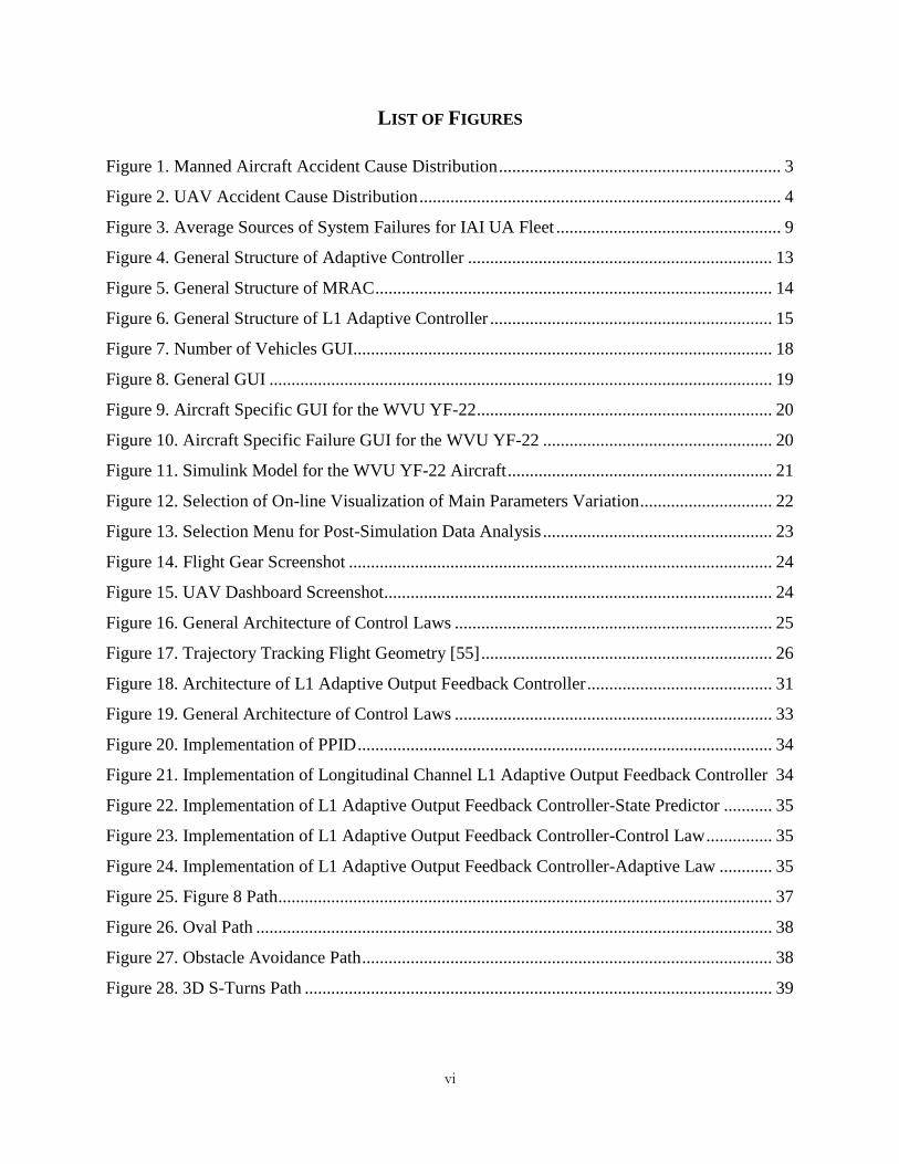
1.2 Failure Statistics of Manned and Unmanned Aircraft
According to FAA, the main threats to aircraft safety are human errors, sensor failures, mechanical
and structural failures, subsystem failures, and adverse weather conditions [15]. FAA has a set of
codes of regulations that is mandatory for all manned aircraft. The FAA certification process
ensures the adequate level for aircraft design and operation safety [16]. As a consequence, the rate
of failure has decreased in recent times for manned aircraft. In the case of UAV, there is no specific
code of regulations and the rate of failure for these systems is one hundred times higher than that
of manned aircraft. The estimated UAV failure rate is one in every one thousand flight hours. This
high failure rate is primarily due to the flexible design methods and low system reliability [17]. To
3
improve the system reliability, significant efforts have been directed towards the development of
fault tolerant control laws in recent years[17].
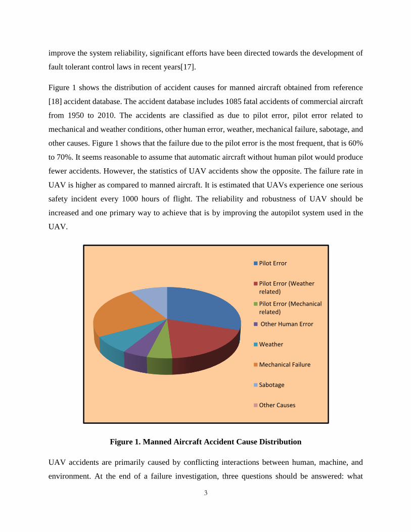
Figure 1 shows the distribution of accident causes for manned aircraft obtained from reference
[18] accident database. The accident database includes 1085 fatal accidents of commercial aircraft
from 1950 to 2010. The accidents are classified as due to pilot error, pilot error related to
mechanical and weather conditions, other human error, weather, mechanical failure, sabotage, and
other causes. Figure 1 shows that the failure due to the pilot error is the most frequent, that is 60%
to 70%. It seems reasonable to assume that automatic aircraft without human pilot would produce
fewer accidents. However, the statistics of UAV accidents show the opposite. The failure rate in
UAV is higher as compared to manned aircraft. It is estimated that UAVs experience one serious
safety incident every 1000 hours of flight. The reliability and robustness of UAV should be
increased and one primary way to achieve that is by improving the autopilot system used in the
UAV.
Figure 1. Manned Aircraft Accident Cause Distribution
UAV accidents are primarily caused by conflicting interactions between human, machine, and
environment. At the end of a failure investigation, three questions should be answered: what
Pilot Error
Pilot Error (Weatherrelated)
Pilot Error (Mechanicalrelated)
Other Human Error
Weather
Mechanical Failure
Sabotage
Other Causes
4
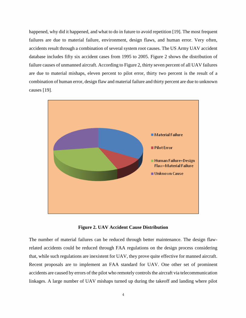
happened, why did it happened, and what to do in future to avoid repetition [19]. The most frequent
failures are due to material failure, environment, design flaws, and human error. Very often,
accidents result through a combination of several system root causes. The US Army UAV accident
database includes fifty six accident cases from 1995 to 2005. Figure 2 shows the distribution of
failure causes of unmanned aircraft. According to Figure 2, thirty seven percent of all UAV failures
are due to material mishaps, eleven percent to pilot error, thirty two percent is the result of a
combination of human error, design flaw and material failure and thirty percent are due to unknown
causes [19].
Figure 2. UAV Accident Cause Distribution
The number of material failures can be reduced through better maintenance. The design flaw-
related accidents could be reduced through FAA regulations on the design process considering
that, while such regulations are inexistent for UAV, they prove quite effective for manned aircraft.
Recent proposals are to implement an FAA standard for UAV. One other set of prominent
accidents are caused by errors of the pilot who remotely controls the aircraft via telecommunication
linkages. A large number of UAV mishaps turned up during the takeoff and landing where pilot
5
commands are directly and critically involved. Alternatively, increasing the autonomy of UAV
through the development and implementation of advanced fault tolerant control laws is expected
to significantly improve the operational safety.
1.3 Control Laws for Autonomous Flight
A critical element for the good performance of UAVs in all their applications consists of following
the required trajectory with good accuracy. Designing trajectory tracking control laws with good
performance and robustness represents a challenging, but critical task. There are two large
categories of controllers: conventional controllers and adaptive controllers. Conventional
controllers use fixed structure and parameters. They are typically designed for limited operational
conditions and rely on intrinsic robustness for adequate operation outside design ranges. Strong
mathematical backgrounds have been developed for this category of control laws that provide
certain levels of guarantees in terms of stability and performance. Adaptive controllers have the
capability to modify their structure and/or the values of their internal parameters according to
changes in the environment. In particular, significant progress has been recorded recently in the
development of control laws that modify the values of their internal gains in response to changes
in the flight conditions, thus featuring a type of dynamic robustness that is very promising ensuring
good performance over the entire flight envelope at both normal and abnormal conditions. The
adaptive controllers are expected to be more robust and reliable; however, a solid theoretical
background is still under construction and consistent certification procedures are still to be
developed and accepted, which currently prevents the adaptive control technologies from being
used in commercial applications.
1.4 Research Objectives
The objective of this research effort is to implement autonomous flight L1 adaptive control laws
in the WVU UAV flight simulation environment and to perform a comparison study between the
L1 adaptive controller and the baseline conventional controller, which relies on position
proportional and integral compensation. Special attention is given to the performance of the
proposed control laws in the presence of abnormal conditions. The abnormal conditions considered
are locked actuators (stabilator, aileron, and rudder) and excessive turbulence. A set of
comprehensive evaluation metrics is used to analyze the performance of autonomous flight control
6
laws in terms of control activity and trajectory tracking errors. It should be noted that the effects
of various factors on the performance of the baseline controller and the adaptive augmentation are
analyzed in order to identify if they have an impact on the relative ranking of the two sets of control
laws. The implementation is performed using MATLAB/Simulink within the WVU UAV
simulation environment [20] [21].
The thesis is organized as follows: Chapter II presents a literature review of current fault tolerant
control laws in manned and unmanned aircraft. This chapter includes a brief introduction to
different controllers and outlines the advantages of the L1 approach over other controllers. Chapter
III describes the architecture of the WVU UAV simulation environment and the integration of L1
within the environment. Chapter IV describes the development of the L1 control laws. This chapter
refers to the mathematical proofs of the L1 controller in the Appendix A. The implementation of
L1 adaptive controller is described in Chapter V. Chapter VI presents the analysis of the
performance of the adaptive control laws. This chapter includes the experimental design, definition
of evaluation metrics, testing, numerical results, and analysis of the performance of L1 versus a
conventional baseline controller. Chapter VII summarizes the conclusions of this research effort
and provides some suggestions for future work involving the L1 adaptive controller.

7
2 LITERATURE REVIEW
2.1 History of UAV
The history of UAV is vast and diverse from the early years of aviation to the current days. The
first UAV can be considered to be the balloon loaded with explosives that flew over Venice in
1849 [22]. In 1916, the first heavier than air UAV, the Hewitt-Sperry Automatic Airplane was
demonstrated. It was named right after the inventors, Hewitt and Sperry [22]. This aircraft become
a reality with the previous work of Sperry on gyroscopic devices that were required to provide
flight stabilization [22]. Other remarkable early UAVs are Curtiss-Sperry Aerial Torpedo and
Liberty Eagle Aerial Torpedo [23].
In Britain, the experiments with UAV begin with RAE Target, in 1921 [23]. The British Royal
Navy used basic radio controlled UAVs, Queen Bee, in 1930. Queen Bee could be landed and
reused and could reach speeds of up to 160 km/h [24]. Queen Bee is the modified version of the
DeHavilland Tiger Moth biplane [22].
Remote operation of aerial vehicles, required the perfection of radio control, which was
proposed in 1895 by Tesla [24]. The private industry “Reginald Denny Hobby Shops” started selling
radio controlled airplanes in 1934. A few years later the US Army developed a successful target
drone which was extensively used during World War II. The SD-1, known as the MQM-57
Falconer, was developed in 1950 [25]. MQM-57 Falconer was remotely operated, carried a camera,
and after a 30 minute flight returned to base and it was recovered using a parachute [25].
The drones for reconnaissance missions by US over China, Vietnam, and other countries in the
1960s and 70s [24] were based on the Ryan Model 147. The Ryan Model 147, also known as the
Lightning Bug, was the first unmanned aircraft that could withstand today’s definition of a UA.
In the meantime, the US Navy acquired a helicopter drone called the QH-50 DASH [23] which
was preferred because it could be launched from smaller vessels. QH-50 DASH was used to launch
antisubmarine torpedoes, to perform surveillance, for cargo transport, and for other applications.
QH-50 DASH was reliable, but still it had issues with its electrical system that led to large number
of losses [25].

8
The Soviet Air Force developed its own reconnaissance drones. A first drone was TBR-1. TBR-1,
was followed by the DBR-1 that allowed for higher range and capabilities [25]. The DBR-1 was
less used because of the operational costs.
In Europe, the unmanned system CL-89 Midge was designed to follow a pre-programmed course,
take photographs and return to base to be recovered by parachute [25]. In the late 1970, the CL-
289 was developed for better performance [25].
Israeli Aircraft Industries developed the Scout and Mastiff [25] in the 70’s. Pioneer, Predator, and
Shadow UAS [26] are based on these designs.
In more recent years, the RQ-4 Global Hawk was designed as a large, high altitude, long endurance
system. The MQ-9 Reaper was specifically designed as a combat UAV or a “hunter killer” and
has been extensively used on battlefields. The DRS-RQ-15 Neptune is a reconnaissance UAV
designed to operate over water. In Britain, the BAE Phoenix is used for combat surveillance, while
the French-built SPERWER supports a number of other European armed forces [26]. In the
Russian Federation, there are several companies involved with UAS development. Although
numerous Unmanned Combat Aircraft Systems (UCAS) are in experimental stages, there are
several that are operational, besides the ones mentioned. They includes the Neuron, the Barracuda,
the Italian Sky-X, the MiG Skat, the General Atomics Avenger, the BAE Mantis, and the Northrop
Grumman X-47 system. UAS based on rotary wing aircraft include the A-160 Hummingbird, the
APID55, the Schiebel S-100, and the MQ-8 Fire scout [26]. A large number of long endurance
systems are also used for civilian applications. For example, NASA employs Helios, Altair, and
Ikhana.
2.2 Types of UAV
There are different types of UAV: target and decoy, reconnaissance, combat, research and
development, civil and commercial. The target and decoy involve the unmanned vehicle used on
earth and in air to destroy the foe vessels. Reconnaissance UAVs are used to gather intelligence,
perform mapping, or assess status after events such as earthquakes or hurricanes. The unmanned
combat air vehicle is used for the high risk missions on the battlefield. The civil and commercial
UAV are uniquely designed for commercial purposes, such as product delivery or advertising. The

9
research and development UAVs provide inexpensive but flexible platforms for design and testing
of new technologies [27].
2.3 UAV Sub-system Failures
Figure 3 shows the source distribution of system failures causing major UAV safety incidents
provided by the International Association for Identification for a RQ-1A/Predator fleet over
100,000 hours of operation in 2002 [28]. The primary sources of catastrophic UAV failures are:
propulsion system, flight controls, human error, and communication system and link.
Figure 3. Average Sources of System Failures for IAI UA Fleet
The most frequent cause for UAV accidents is power or propulsion failure, which occurs due to
mishaps in the engine, provision of power, transmission, propeller, electrical system, generators,
or other secondary devices. From Figure 3, it is estimated that thirty two percent of the total number
of failures are propulsion failures. For example, the solar powered Helios crashed during a test
flight in 2003. The test was carried out at night to ensure that the solar powered wing can manage
to deliver the power without any interruption. The planned flight was about forty hours but the
Helios crashed into the Pacific Ocean near the island of Kauai [29]. An MQ-1B Predator collapsed
on Aug 22, 2012 in Afghanistan. According to [30] report mishap was due to failure of dual
alternator.

10
The second frequent failure affects the flight control system. The flight control devices include
avionics, air data system, servo-actuators, control surfaces, on-board software, navigation
instrumentation, and other associated accessories. For example, the experimental X-51A crashed
into the Pacific Ocean on 14 August, 2012 due to a failure of the control fin. After sixteen seconds
into the flight, sensors detected the malfunction of the control fin, which prevented the crew from
maintaining control of the aircraft [31]. Actuator failures may include locked control surface,
missing or damaged control surface, free floating surface, reduced control effectiveness, or
combinations of them. Actuator failures affect primarily the linkage system and the aerodynamic
control surfaces. They can occur due to a variety of causes ranging from collision with an external
object to acute structural failures with calamitous separation of elements. The RQ-4A Global
Hawk UAV crashed on June 11, 2012 near the Naval Air Station Patuxent River in Maryland
during flight training. The accident occurred because of the failure of the right ruddervator actuator
[32]. Sometimes the source of the actuator malfunction may reside with the ground station. The P-
175 Polecat UAV crashed during a Nevada test in December 2006 [33]. During the flight, the
primary console PPO-1 locked up and it was necessary to switch to the back-up console PPO-2.
When switching between two consoles, the control configurations of the two consoles should
match. It didn’t happen that day, resulting in a fuel cut off position that lead to the accident [33].
A drone crashed during a trip to Panama because of human error, the next category of most
frequent UAV accident causes. The crew set the drone to 'fly-by-wire' instead of 'receiver failsafe'.
As soon as the UAV flew out of radio range, control was lost and the aircraft collapsed within
seconds [33].
The fourth most common cause of UAV incidents is the malfunction of the communication link
between UAV and the ground station. For example, an MQ-1B Predator crashed on September 18,
2012 due to failure of the satellite data link [30].
Several other miscellaneous sources such as operating and scheduling problems, non-technical
factors, or weather are also reported to produce major incidents and accidents [34].
2.4 Controllers
Autopilots or automatic pilots are devices for controlling the vehicles without constant human
intervention [35]. These control systems are typically categorized as conventional or fixed-

11
parameter controllers and adaptive controllers. A typical commonly used architecture for trajectory
tracking consists of an inner/outer loop structure [36] [37]. The inputs to the outer loop are
trajectory-defining variables such as waypoints and desirable vehicle velocity. Kinematic
equations are used to obtain necessary attitude angles and rates, which are the inputs to the inner
loop. These are then converted into deflections of the aircraft aerodynamic control surfaces.
2.4.1 Conventional Controllers
Conventional controllers play a vital role in the industry because of their transparent structure,
simplicity, and adequate performance. Extensive theoretical background and design
methodologies are typically available for a variety of different approaches [38], such as pole
placement, linear quadratic optimal regulator controller and proportional, integral, and derivative
(PID) [39].
The pole placement or pole assignment technique is a linear approach based on locating the poles
of the closed loop system such that the desirable dynamic response is ensured. It is applicable to
systems that are completely observable and controllable. A dynamic feedback linear controller
using pole placement and Kalman filtering is used to control a UAV in [40]. In many problems,
exact pole placement is not necessary, it is sufficient to locate the pole of the closed loop system
in a sub-region of the complex left half plane [41].
Linear quadratic control approaches have been widely used for both fixed wing [42] and rotary
wing UAVs [43]. The linear quadratic regulator (LQR) has been demonstrated to be effective in
numerous UAV applications [44]. In [45] a gain-scheduled LQR controller is developed for an
autonomous airship. The augmentation of LQR control laws with Kalman filtering has been shown
to improve disturbance rejection and the overall effectiveness of the control system [46].
Due to their simplicity, effectiveness, and solid theoretical background, PID controllers are a very
popular solution for UAV applications [47] [48], including fixed wing [49], rotary wing [50],
quadrotors [51] [52] [53], and lighter-than-air UAVs [54]. Both inner and outer loop can be
designed based on PID compensation [49]. A simple approach uses altitude and heading as inputs;
however, better tracking performance can be achieved with waypoint inputs [55].

12
Kinematic and dynamic aircraft models can be used to obtain the required states and controls given
desired position and velocity, through a model inversion process [56]. Typically, inversion is used
for the outer loop, while other control design methods are used for the inner loop [57] [58] [59].
However, improved performance can be obtained if the inversion approach is extended to the inner
loop as well [60].
2.4.2 Adaptive Controllers
An adaptive controller has the capability to modify its structure and/or parameters (gains)
depending on current operational conditions. While modifying the structure of the controller is
possible, most design methodologies for adaptive control systems consider only the variation of
the gains. Aircraft operate over wide ranges of speed and altitude and their dynamics are time
varying and non-linear. This makes them primary candidates to benefit from adaptive control laws.
Control system design in linear domain requires that, for a given aircraft speed and altitude, the
complex dynamic equations are approximated by a linear model. For example, at operating point
i, the equations of motion are:
�̇�(𝑡) = 𝐴𝑖𝑥(𝑡) + 𝐵𝑖𝑢(𝑡), 𝑥(0) = 𝑥0, (1)
𝑦(𝑡) = 𝐶𝑖𝑇𝑥(𝑡) + 𝐷𝑖𝑢(𝑡) (2)
where 𝐴𝑖,𝐵𝑖,𝐶𝑖,𝐷𝑖 are state space constant matrices at operating point. As the aircraft flies to a
different operating point, these matrices change. The control system designed for one operating
point may not be adequate at a different operating point. Therefore, the parameters of the control
laws must be adjusted depending on current operational conditions. Figure 4 shows the feedback
controller with adjustable gains and the plant. A variety of methodologies can be used to achieve
the variation of the controller gains in response to variations in the plant and external conditions
[61].

13
Figure 4. General Structure of Adaptive Controller
Gain scheduling [62] [63] can be considered as the simplest adaptive technique. It consists of
selection and use of appropriate gains from a set of gain values that has been pre-computed. By
selecting suitable gain values depending on the operating point, the performance of the controller
may be greatly improved. The previously designed linear controllers may each satisfy strict
robustness and performance criteria at a given operating point. The advantage of gain scheduling
resides in the potential of achieving optimal operation at the design operating points. One
significant disadvantage of the approach is the need for, possibly, frequent and rapid changes of
controller gains, which may deteriorate performance in the transition and even lead to instability.
One other limitation is the high design and implementation costs, which increase rapidly with the
number of operating points.
One of the most popular methods for aircraft control system design is feedback linearization. The
non-linear dynamic inversion (NLDI) [64] calculates the non-linear control signal using an inverse
transformation. For a high fidelity plant model, the cancellation of non-linearity is achieved
through the transformation. However, for high-performance practical applications, modeling
uncertainties and errors must be compensated for by using adaptation mechanisms. Artificial
neural networks [65] have been used to augment NLDI control laws [66]. The artificial neuron is
a simple computational unit inspired by the biological neuron. In a similar manner as its biological
counterpart, the artificial neural network possesses significant capabilities for distributed
information processing and parallel computing [67]. It can accurately approximate complicated
multi-dimensional non-linear functions by “learning” the input/output relationships of large sets
of experimental data. Therefore, it can model and predict complex dynamics and provide adequate
Strategy for Adjusting
Controller Gains
Plant Controller
𝐼𝑛𝑝𝑢𝑡 𝑐𝑜𝑚𝑚𝑎𝑛𝑑
𝑢(𝑡) 𝑦(𝑡)
14
adaptive control compensation when the controlled system changes due to external or internal
conditions [68].
Fuzzy logic [69] has been used for aircraft adaptive control including UAV. As opposed to binary
logic where a statement can only be true or false, within fuzzy logic, a statement can be true, false,
or anything in between. This allows the transfer of human operator control experience formulated
through common language as “IF-THEN” conditional propositions. Fuzzy logic has been applied
to nonlinear systems [70], which lack complete analytical models. The dynamics of a system can
be constructed from knowledge of similar systems using fuzzy logic arguments, and a fuzzy
controller can be constructed via conditional proposition decisions [71] [72].
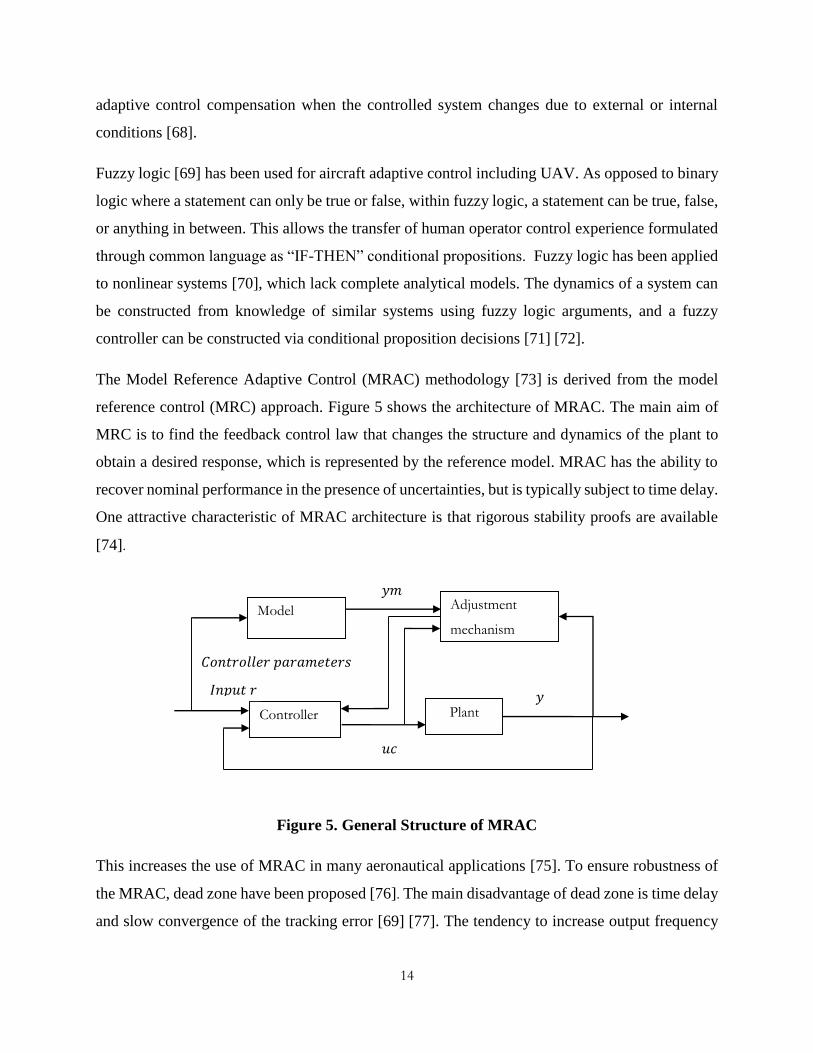
The Model Reference Adaptive Control (MRAC) methodology [73] is derived from the model
reference control (MRC) approach. Figure 5 shows the architecture of MRAC. The main aim of
MRC is to find the feedback control law that changes the structure and dynamics of the plant to
obtain a desired response, which is represented by the reference model. MRAC has the ability to
recover nominal performance in the presence of uncertainties, but is typically subject to time delay.
One attractive characteristic of MRAC architecture is that rigorous stability proofs are available
[74].
Figure 5. General Structure of MRAC
This increases the use of MRAC in many aeronautical applications [75]. To ensure robustness of
the MRAC, dead zone have been proposed [76]. The main disadvantage of dead zone is time delay
and slow convergence of the tracking error [69] [77]. The tendency to increase output frequency
Model Adjustment
mechanism
Plant Controller
𝑦 𝐼𝑛𝑝𝑢𝑡 𝑟
𝐶𝑜𝑛𝑡𝑟𝑜𝑙𝑙𝑒𝑟 𝑝𝑎𝑟𝑎𝑚𝑒𝑡𝑒𝑟𝑠
𝑦𝑚
𝑢𝑐

15
of the control unit increases the adaptation rate. As a consequence, the speed of convergence
decreases [78]. To mitigate these issues, a filtered version of MRAC has been proposed known as
L1 adaptive controllers [79] [80] [81]. Figure 6 shows the architecture of L1 adaptive controller.
The low pass filter used in L1 ensures a bandwidth limited control signal and high adaptation rate
[82] [83]. The main advantage of L1 adaptive controller over MRAC is that L1 clearly separates
performance, robustness, and high adaptation rate [84]. The L1 architecture permits robustness of
the system in the presence of fast adaptation. L1 adaptive control has three distinct components.
First, a state predictor law models the system’s desired performance. Second, an adaption law
ensures the plant and state estimates are same. Finally, a control law utilizes a low pass linear filter
to eliminate high frequency in the control channel. This allows the use of high gains without the
adverse effect on robustness.
Figure 6. General Structure of L1 Adaptive Controller
L1 control could be implemented to obtain faster response compared with the conventional
methods. The design of L1 adaptive controller reduces tuning of gains to achieve desired
characteristics in presence of failures. The techniques used for the convergence are Lyapunov or
passivity techniques and averaging theory [85] [86] [87] [88]. The Lyapunov method of developing
adaptive laws is based on the direct method of Lyapunov and its relationship with positive real
functions [89] [90] [91] [92]. In this method, the problem of designing an adaptive law is
approached as a stability problem where the differential equation of the adaptive law is chosen
such that certain stability conditions based on Lyapunov theory are satisfied. In addition, some
Model Adjustment
mechanism
Plant Controller+
LP Filter
𝑦 𝐼𝑛𝑝𝑢𝑡 𝑟
𝐶𝑜𝑛𝑡𝑟𝑜𝑙𝑙𝑒𝑟 𝑝𝑎𝑟𝑎𝑚𝑒𝑡𝑒𝑟𝑠
𝑦𝑚
𝑢𝑐

16
studies suggest that the Lyapunov-based adaptive control schemes achieve higher performance
than MIT rule-based schemes [93] [94] [95] [96] [97] [98].
L1 has been successfully demonstrated on drilling systems [99], wing rock compensation [100],
and other flight control systems [55]. Additionally, adaptive control has been successful tested on
NASA’s AirSTAR test vehicle [101]. On June 2nd 2010, a test flight of the AirSTAR was
performed with an all-adaptive flight control system in Fort Pickett, VA. The adaptive controller
guaranteed safe operation of the vehicle during the flight, and the pilot satisfactorily flew the
specified tasks.

17
3 WVU UAV SIMULATION ENVIRONMENT
The WVU UAV simulation environment is developed in MATLAB and Simulink to provide
maximum flexibility and portability and allow for easy updating, extension, and implementation
of new algorithms. The simulation environment is interfaced with Flight Gear [102] software
package for visualization and with a C# customized map generator and visual feedback
environment referred to as UAV dashboard [103] .
The WVU UAV Simulation environment currently includes five aircraft models. Each aircraft
model is connected within a specific Simulink model. Nonlinear equations of motion and
aerodynamic models are implemented. The Simulink block of each aircraft accepts pilot control
commands such as elevator, aileron, rudder, and throttle and inputs from the outside environment
like steady wind, gusts, and turbulence. A variety of sensor, actuator, and propulsion system
failures, as well as structural damages can be simulated. Extensive on-line data visualization and
recording for later analysis are available. The simulation environment is a valuable tool for UAV
control system design, verification, analysis, and comparison. Path planning and trajectory
tracking are critical parts of the simulation environment. Several path planning algorithms are
implemented ranging from simple grid-based approaches 3-dimensional Dubins and clothoid-
based methods. Several trajectory tracking algorithms included in the simulation environment are
designed to possess fault tolerant capabilities in the presence of abnormal conditions. Both fixed-
parameter or conventional algorithms and variable-parameter or adaptive algorithms are
implemented.
3.1 Graphical User Interface (GUI) for Simulation Setup
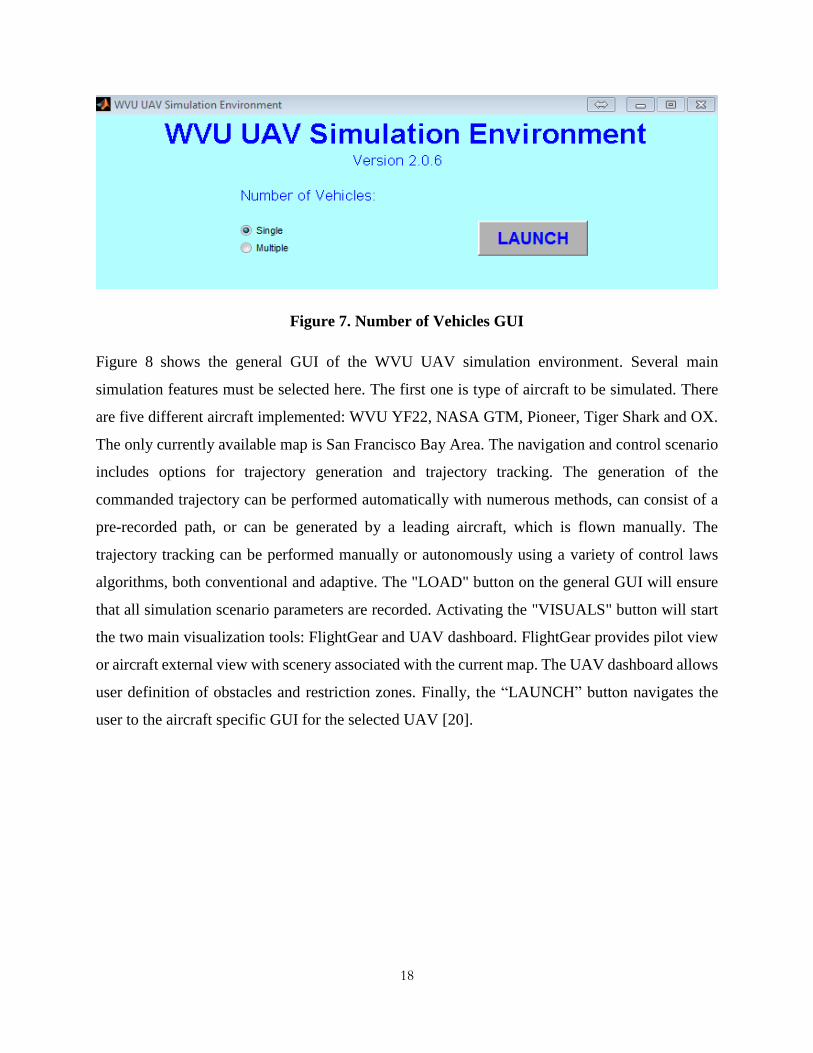
The first step in operating the WVU UAV simulation environment is to setup the simulation
scenario and initialize all the necessary variables. The Matlab script "WVUUAV.m" is executed
first. It prepares the Matlab work space and opens the first interactive menu for the selection of a
single or multiple vehicle simulation session. This menu is presented in Figure 7. It directs to the
general GUI, where the user can select the other necessary parameters to run the simulation. The
user is required to provide input on the general GUI for each of the vehicles involved in the
simulation.
18
Figure 7. Number of Vehicles GUI
Figure 8 shows the general GUI of the WVU UAV simulation environment. Several main
simulation features must be selected here. The first one is type of aircraft to be simulated. There
are five different aircraft implemented: WVU YF22, NASA GTM, Pioneer, Tiger Shark and OX.
The only currently available map is San Francisco Bay Area. The navigation and control scenario
includes options for trajectory generation and trajectory tracking. The generation of the
commanded trajectory can be performed automatically with numerous methods, can consist of a
pre-recorded path, or can be generated by a leading aircraft, which is flown manually. The
trajectory tracking can be performed manually or autonomously using a variety of control laws
algorithms, both conventional and adaptive. The "LOAD" button on the general GUI will ensure
that all simulation scenario parameters are recorded. Activating the "VISUALS" button will start
the two main visualization tools: FlightGear and UAV dashboard. FlightGear provides pilot view
or aircraft external view with scenery associated with the current map. The UAV dashboard allows
user definition of obstacles and restriction zones. Finally, the “LAUNCH” button navigates the
user to the aircraft specific GUI for the selected UAV [20].

19
Figure 8. General GUI
The model of WVU YF-22 will be used within this research effort. This aircraft is a small UAV
powered by a miniature jet engine with limited fuel capacity allowing about 12 minutes of flight
[21]. The WVU YF-22 research UAV was designed based on the prototype of the U.S Air
Lockheed/Boeing F-22 fighter aircraft. The aim of designing the WVU UAV was mainly for
testing various fault tolerant control algorithms in flight.
Several path planning algorithms are included in the WVU UAV Simulation environment. Some
allow for risk zone avoidance, while others ensure that desired points of interest are reached. A
variety of different approaches are implemented ranging from grid, Voronoi, and potential field
methods to 2- and 3-dimensional Dubins and clothoid-based methods. For more information about
20
these algorithms, refer to [104]. In this research, different 2-D and 3-D recorded paths were
considered [105].
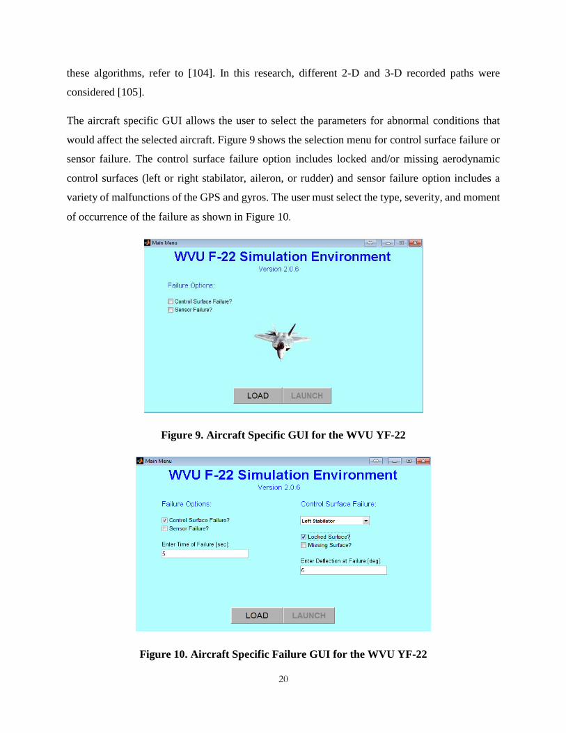
The aircraft specific GUI allows the user to select the parameters for abnormal conditions that
would affect the selected aircraft. Figure 9 shows the selection menu for control surface failure or
sensor failure. The control surface failure option includes locked and/or missing aerodynamic
control surfaces (left or right stabilator, aileron, or rudder) and sensor failure option includes a
variety of malfunctions of the GPS and gyros. The user must select the type, severity, and moment
of occurrence of the failure as shown in Figure 10.
Figure 9. Aircraft Specific GUI for the WVU YF-22
Figure 10. Aircraft Specific Failure GUI for the WVU YF-22
21
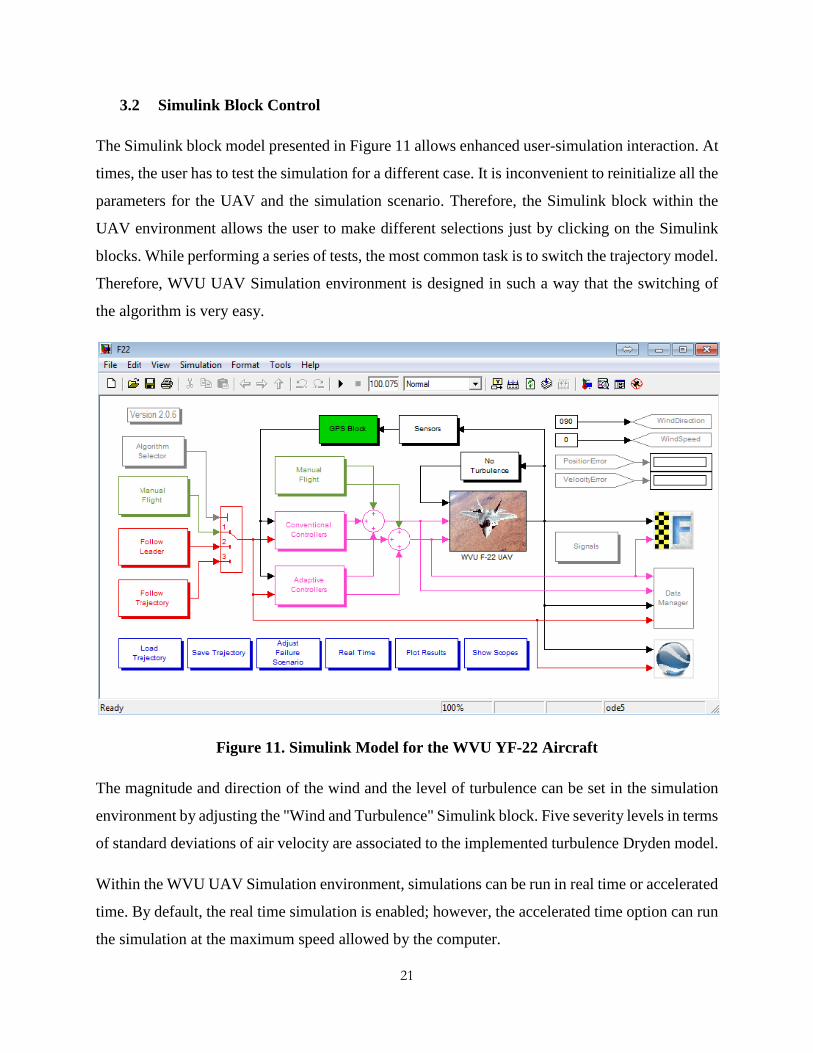
3.2 Simulink Block Control
The Simulink block model presented in Figure 11 allows enhanced user-simulation interaction. At
times, the user has to test the simulation for a different case. It is inconvenient to reinitialize all the
parameters for the UAV and the simulation scenario. Therefore, the Simulink block within the
UAV environment allows the user to make different selections just by clicking on the Simulink
blocks. While performing a series of tests, the most common task is to switch the trajectory model.
Therefore, WVU UAV Simulation environment is designed in such a way that the switching of
the algorithm is very easy.
Figure 11. Simulink Model for the WVU YF-22 Aircraft
The magnitude and direction of the wind and the level of turbulence can be set in the simulation
environment by adjusting the "Wind and Turbulence" Simulink block. Five severity levels in terms
of standard deviations of air velocity are associated to the implemented turbulence Dryden model.
Within the WVU UAV Simulation environment, simulations can be run in real time or accelerated
time. By default, the real time simulation is enabled; however, the accelerated time option can run
the simulation at the maximum speed allowed by the computer.

22
Simulink on-line scopes can be used to visualize certain parameters and their variations in real
time. As shown in Figure 12, there are 22 scopes that are used to visualize a variety of state,
controlled, and control variables. In addition to this, after the simulation, several plots can be
generated allowing for the investigation of particular parameters. Figure 13 presents the selection
menu for post-simulation data presentation and analysis. Time histories are generated for significant
variables such as the 2-D and 3-D trajectory, controller errors, aircraft states, and pilot commands.
Within the data manager block all these variables, are also saved to disk for later use and analysis.
Figure 12. Selection of On-line Visualization of Main Parameters Variation
At times, it is very useful to manually fly a certain trajectory and save it for consequent evaluation
of trajectory tracking algorithms. The trajectory generated in this way can be saved and used later
as a commanded trajectory. Pre recorded paths generated manually or analytically are stored in a
library and can be used for trajectory tracking algorithm testing. The interactive windows for
FlightGear and UAV Dashboard can be opened from the Simulink model without going through
the GUI setup process.

23
Figure 13. Selection Menu for Post-Simulation Data Analysis
3.3 Flight Path Visualization
Within the WVU UAV simulation environment, the flight path visualization is performed using
Flight-Gear and UAV Dashboard. The Flight-Gear software package is used to visualize the 3-D
motion of the UAV in a high quality visual environment. Figure 14 presents an example of external
visual cues provided by Flight-Gear. Figure 15 shows the UAV dashboard utility, which generates
the flight map, allows the user to locate obstacles and risk zones, and displays both the commanded
and the actual 2-dimensional aircraft trajectory. Obstacle configurations can be saved and re-used
for repeated tests under modified conditions. The UAV Dashboard shows the position and
orientation of the moving UAVs with respect to the risk zones allowing the user to qualitatively
evaluate the performance of the controllers.

24
Figure 14. Flight Gear Screenshot
Figure 15. UAV Dashboard Screenshot

25
4 PROBLEM FORMULATION
The main challenge of autonomous flight consists of accurately tracking the trajectory under
normal and adverse conditions. In this thesis, L1 adaptive control laws have been implemented
and analyzed within the WVU UAV simulation environment. The L1 adaptive components
augment a conventional position proportional integral and derivative (PPID) baseline controller
and a performance comparison is performed between the baseline and the augmented set of control
laws. The proposed adaptive control laws are based on inner-outer loop control architecture as
presented in Figure 16. The three main components (trajectory geometry, outer loop, and inner
loop) are described next.
Figure 16. General Architecture of Control Laws
4.1 Geometry of the Trajectory Tracking Problem
The trajectory variable calculation can be separated into two problems: a horizontal-plane tracking
problem and a vertical-plane tracking problem, as shown in Figure 17. The forward distance error
f and lateral distance error l can be calculated from position and velocity using the following
relationships:
𝑙 =
𝑉𝐿𝑦(𝑥𝐿 − 𝑥𝑤) − 𝑉𝐿𝑥(𝑦𝐿 − 𝑦𝑤)
𝑉𝐿𝑥𝑦− 𝑙𝑐 (3)
𝑓 =
𝑉𝐿𝑥 (𝑥𝐿 − 𝑥𝑤) + 𝑉𝐿𝑦 (𝑦𝐿 − 𝑦𝑤 )
𝑉𝐿𝑥𝑦− 𝑓𝑐 (4)
Trajectory Variable Calculation
Outer-loop Controller
Inner-loop Controller
𝑥𝑑
𝑦𝑑
𝑧𝑑
ℎ, ℎ̇
𝐼, 𝐼 ̇
𝑓, 𝑓̇
𝜃𝑑
∅𝑑
𝛿𝑒
𝛿𝑎
𝛿𝑟
𝛿𝑇
Aircraft
Dynamics

26
where 𝑉𝐿𝑥𝑦 = √𝑉𝐿𝑥2 + 𝑉𝐿𝑦
2 is the projection of desired trajectory velocity onto x-y plane 𝑉𝐿𝑥 , 𝑉𝐿𝑦
are the projections of reference trajectory along x and y axes of Earth fixed frame; 𝑙𝑐 and 𝑓𝑐, are
clearance parameters. The clearance parameters will be zero for the purpose of this study.
Figure 17. Trajectory Tracking Flight Geometry [88]
Therefore, the lateral distance error l and the forward distance error f can further be expressed as:
[𝑙𝑓] = [
𝑠𝑖𝑛 (𝜒𝐿) −𝑐𝑜𝑠 (𝜒𝐿)𝑐𝑜𝑠 (𝜒𝐿) 𝑠𝑖𝑛 (𝜒𝐿)
] [𝑥𝐿 − 𝑥𝑦𝐿 − 𝑦] (5)
where 𝜒𝑉 is given by:
𝑐𝑜𝑠(𝜒𝑉) =𝑉𝐿𝑥
√𝑉𝐿𝑥2+𝑉𝐿𝑦
2 and 𝑠𝑖𝑛(𝜒𝑉) =
𝑉𝐿𝑦
√𝑉𝐿𝑥2+𝑉𝐿𝑦
2 (6)
The relative forward and lateral speeds of aircraft are obtained from time derivatives of the forward
and lateral distance, respectively:

27
𝑙̇ =
𝑉𝐿𝑥𝑉𝑤𝑦 − 𝑉𝐿𝑦𝑉𝑤𝑦
𝑉𝐿𝑥𝑦+ 𝛺𝐿𝑓 (7)
𝑓̇ = 𝑉𝐿𝑥𝑦 −
𝑉𝐿𝑥 𝑉𝐿 − 𝑉𝐿𝑤 𝑉𝑤
𝑉𝐿𝑥𝑦+ 𝛺𝐿𝑙 (8)
where 𝛺𝐿 =(𝑞𝐿 sin𝜙𝐿+𝑟𝐿 cos𝜙𝐿)
cos 𝜃𝐿 is the trajectory projected angular velocity in the x-y plane, which
is assumed to be zero. Equations (7) and (8) can be written as:
[𝑙̇
𝑓̇] = [𝑉𝑥𝑦 sin(𝜒 − 𝜒𝑉)
𝑉𝑉𝑥𝑦− 𝑉𝑥𝑦 cos(𝜒 − 𝜒𝑉)
] + 𝛺𝐿 [𝑓−𝑙
] (9)
For the vertical geometry, the vertical distance error h and vertical speed h can be calculated as:
ℎ = 𝑧𝐿 − 𝑧𝑤 (10)
ℎ̇ = 𝑉𝐿𝑥 − 𝑉𝑤𝑥 (11)
4.2 Outer Loop Controller
The outer loop controller used is the positional proportional integral and derivative controller. The
PPID gains have been optimized with an evolutionary algorithm [86] using as optimization
criterion a combined performance index based on tracking errors and control activity. The outer
loop controller is expected to convert position commands on the three channels (longitudinal,
lateral, and vertical) into required throttle, bank angle, and pitch angle, respectively. Proportional
and integral relationships are used for this purpose. Equation (12), Equation (13) and Equation
(14) represents the generation of the desired bank angle, throttle command and pitch angle.
𝜙𝑑 = 𝐾𝑙̇𝑙̇ + 𝐾𝑙𝑙 (12)
𝛿𝑇 = 𝐾�̇��̇� + 𝐾𝑓𝑓 (13)
𝜃𝑑 = 𝐾ℎ̇ℎ̇ + 𝐾ℎℎ (14)
28
4.3 Inner Loop Controller
The inner loop is expected to generate the aerodynamic control surface deflections necessary to
achieve the commanded bank and pitch angles produced by the outer loop. Two different
approaches for the inner loop are involved in this study: PPID [55], and L1 adaptive feedback [87]
[79] [80]. The implemented L1 adaptive controller in WVU UAV Simulation environment is
different from the previous implementations in terms of the design and parameters of the L1 filter
as well as additional compensation on the yaw channel.
4.3.1 Proportional Integral Derivative Controller
The desired aileron, rudder and elevator deflections are obtained using primarily the desired bank
angle, yaw rate, and desired pitch angle, respectively.
The lateral controller generates aileron and rudder deflection using equations (15) and (16).
𝛿𝑎 = 𝐾𝑝𝑝 + 𝐾𝜙(𝜙 − 𝜙𝑑) (15)
𝛿𝑟 = 𝐾𝑟𝑟 (16)
Equation (17) provides the elevator deflection using the desired pitch angle and pitch rate.
𝛿𝑒 = 𝐾𝑞𝑞 + 𝐾𝜃(𝜃 − 𝜃𝑑) (17)
where p, q, r, ϕ are the actual roll rate, pitch rate, yaw rate and bank angle respectively, 𝜙𝑑 and 𝜃𝑑
are the desired bank and pitch angles.
4.3.2 Architecture of L1 Adaptive Feedback Controller
The first step in the development of L1 adaptive control laws is the creation of a linear model of
the UAV [87] [79] [80]. The desired natural frequency and damping ratio of the longitudinal and
lateral channels are found, in order to create the reference system.
L1 adaptive controller can be designed following the assumption of decoupled longitudinal and
the lateral-directional aircraft dynamics. This implies that the dynamics of the vehicle can be
expressed by two different decoupled linear systems shown below:

29
𝑥𝑙𝑜𝑛̇ (𝑡) = 𝐴𝑙𝑜𝑛𝑥𝑙𝑜𝑛(𝑡) + 𝐵𝑙𝑜𝑛𝑢𝑙𝑜𝑛(𝑡) (18)
𝑥𝑙𝑎𝑡̇ (𝑡) = 𝐴𝑙𝑎𝑡𝑥𝑙𝑎𝑡(𝑡) + 𝐵𝑙𝑎𝑡𝑢𝑙𝑎𝑡(𝑡) (19)
The longitudinal and lateral systems are independent. The states and the control input vectors of
the longitudinal dynamics are given below
𝑥𝑙𝑜𝑛 = [𝑣 𝛼 𝑞 𝛳]𝑇 (20)
𝑢𝑙𝑜𝑛 = 𝛿𝑒 (21)
where the states are velocity, angle of attack, pitch rate, and pitch attitude angle. The control 𝛿𝑒 is
the deflection of the elevator.
The states and the control input vectors of the lateral-directional dynamics are given below:
𝑥𝑙𝑎𝑡 = [𝛽 𝑝 𝑟 𝜙]𝑇 (22)
𝑢𝑙𝑎𝑡 = [𝛿𝑎𝛿𝑟]𝑇 (23)
where the states are sideslip angle, roll rate, yaw rate, and roll attitude angle and the inputs are
𝛿𝑎, deflection of the aileron and 𝛿𝑟, the deflection of the rudder.
The state space equations of the aircraft (WVU YF-22) are obtained from reference [88]. The
linear model is obtained at a steady state and level flight with V= 42 m/s H=120m at trim
conditions 𝛼 = 𝛳 = 3𝑜 with 𝛿𝑒=-1°, 𝛿𝑎=𝛿𝑟=0 and thrust force along x axis T=54.62N. Since the
inner loop does not process the turbulence, the created reference model uses the actuator
deflections as input.
The resultant continuous time longitudinal and lateral-directional linear models are:
[
�̇��̇��̇�
�̇�
] = [
−0.2835 −23.09590 −4.1172 0 −33.88360 0
0 −0.1711 0.7781 0
−3.5729 01 0
] [
𝑣𝛼𝑞𝛳
]
+ [
20.16810.5435
−39.08470
] 𝛿𝑒
(24)

30
[ �̇��̇��̇��̇�]
= [
0.4299 0.0938−67.3341 −7.948520.5333 −0.6553
0 1
−1.0300 0.23665.6402 0
−1.9955 00 0
] [
𝛽𝑝𝑟𝜙
] + [
0.2724 −0.7713−101.8446 33.4738−6.2609 −24.3627
0 0
] [𝛿𝑎
𝛿𝑟] (25)
From this, the necessary natural frequency and damping ratio of the longitudinal and lateral
channels are the following: 𝜔𝑞 = 4.5, 𝜁𝑞 = 0.7 𝜔𝑟 = 4.2, 𝜁𝑟=0.4
The reference models 𝑀𝑞(𝑠) and 𝑀𝑟(𝑠) are designed such that desired dynamic response is
achieved.
𝑀𝑞 =
𝜔𝑞2
𝑠2 + 2𝜁𝑞𝜔𝑞 + 𝜔𝑞2 (26)
𝑀𝑟 =
𝜔𝑟2
𝑠2 + 2𝜁𝑟𝜔𝑟 + 𝜔𝑟2 (27)
The architecture of the L1 adaptive controller is described in Figure 18 . L1 adaptive controller
consists of three blocks: control law, state predictor, and adaptive law.
The state predictor estimates the system output. Consider that the desired output of the system is
expressed as:
𝜃(𝑠) = 𝑀𝑞(𝑠)(𝜃𝑎𝑑(𝑠) + 𝜎𝑞(𝑠)) (28)
where 𝜎𝑞(𝑠) includes the uncertainty of the plant and its departure from the desired response and
𝜃𝑎𝑑(𝑡) is the compensation produced by the control law.

31
Figure 18. Architecture of L1 Adaptive Output Feedback Controller
The state space system of equations is given as:
�̇�(𝑡) = Amq𝑥(𝑡) + Bmq
(𝜃𝑎𝑑(𝑡) − 𝜎𝑞𝑥(𝑡)) (29)
𝜃(𝑡) = Cmq
𝑇𝑥(𝑡) (30)
The state predictor is formulated as:
�̂̇�(𝑡) = Amq�̂�(𝑡) + Bmq
𝜃𝑎𝑑(𝑡) + �̂�𝑞(𝑡) (31)
𝜃(t) = Cmq
𝑇�̂�(𝑡) (32)

32
where �̂�𝑞(t) ϵ R*R is the result of the adaptation. Note also that, Amq, Bmq
, Cmq
𝑇 are the minimal
realization of 𝑀𝑞(𝑠) in controllable canonical form. The adaptive law estimates �̂�𝑞(𝑡) are given
as:
�̂�𝑞(𝑖𝑇) = −(∫ 𝑒𝛬𝑞Amq𝛬𝑞
−1(𝑇−𝜏)𝛬𝑞𝑑𝜏
𝑇
0
)−1(𝑒𝛬𝑞Amq𝛬𝑞−1(𝑇−𝜏)
𝐼1�̃�(𝑖𝑇)) (33)
where 𝐼1 = [0 1], 𝛬𝑞 = [𝐶𝑚𝑞
𝑇
𝐷𝑞√𝑝𝑞
], i is the sample index and the estimation error is �̃�(𝑡) = 𝜃(t) −
θ(t), while T is signal sampling time interval. 𝑝𝑞 is the solution to the algebraic Lyapunov equation
Amq
𝑇𝑝𝑞 + 𝑝𝑞Amq= −Qq, where Qq = |
1 00 0
|. The obtained 𝑝𝑞 should satisfy the condition:
𝑝𝑞 = √𝑝𝑞𝑇√𝑝𝑞. 𝐷𝑞 is the nullspace of 𝐶𝑚𝑞
𝑇(√𝑝𝑞)−1, that is 𝐷𝑞(𝐶𝑚𝑞
𝑇(√𝑝𝑞)−1)𝑇 = 0.
The control law generates θad and is given as:
θad(s) = Cq(s)rq(s) −
Cq(s)
Mq(s)cmqT (sI − Amq
)−1
�̂�𝑞(s) (34)
where rq(t) is a bounded reference signal with bounded first and second order derivatives. cq(s)
is a strictly proper low pass filter with Cq(0)=1 such that Cq(s)
Mq(s)Cmq
T (sI − Amq)−1
is a proper
transfer function. A low pass filter offers easy passage to low frequency signal and attenuates high
frequency signal components. The low pass filter eliminates external or internal disturbances
faster. The effect of adding the low pass filter consists in limiting the bandwidth of the control
signal. Larger gains and hence faster adaptation and response are possible, without penalty on
robustness.

33
5 IMPLEMENTATION OF L1 ADAPTIVE CONTROLLER
The Simulink implementation of the L1 adaptive control laws is organized in three main blocks:
trajectory variable calculation, outer loop controller and inner loop controller. Figure 19 represents
the general implementation of the control laws. The aircraft actual states and the commanded path
are used as input to the trajectory variables calculation. The outer loop calculates the required bank
angle, pitch angle, and the throttle command. The inner loop controller generates the deflections
of lateral and longitudinal aerodynamic control surfaces.
Figure 19. General Architecture of Control Laws
The first implementation is the inner loop PPID followed by the implementation of L1 adaptive
output feedback controller. Figure 20 represents the implementation of PPID. The pitch angle and
bank angle are used to generate deflections of elevator, rudder, and aileron. Figure 21 represents
the implementation of L1 adaptive output feedback controller on the longitudinal channel. The
architecture of the lateral channel implementation is the same.

34
Figure 20. Implementation of PPID
Figure 21. Implementation of Longitudinal Channel L1 Adaptive Output Feedback
Controller
The implementations of the state predictor, control law and adaptive law are shown in

35
Figure 22, Figure 23, and Figure 24, respectively. From these figures, it can be clearly seen that
the L1 output feedback adaptive controller uses the pitch angle in the feedback loop.
Figure 22. Implementation of L1 Adaptive Output Feedback Controller-State Predictor
Figure 23. Implementation of L1 Adaptive Output Feedback Controller-Control Law
Figure 24. Implementation of L1 Adaptive Output Feedback Controller-Adaptive Law
36
6 PERFORMANCE ANALYSIS
In order to assess the impact of the L1 adaptive control laws and their fault tolerance capabilities,
the L1 adaptive controller and the PPID control laws were tested at nominal conditions and under
a variety of abnormal conditions. The performance evaluation metrics used are expected to be
comprehensive with respect to critical elements of autonomous flight performance, such as
trajectory tracking and control activity. The use of weighting factors may introduce some
subjectivity; however, this is mitigated by considering component performance indices in on
conjunction with global ones. The experimental design has considered 4 different paths with
different levels of complexity and locked actuator failures on all control channels as well as
turbulence. The abnormal conditions were evaluated at three different levels of severity.
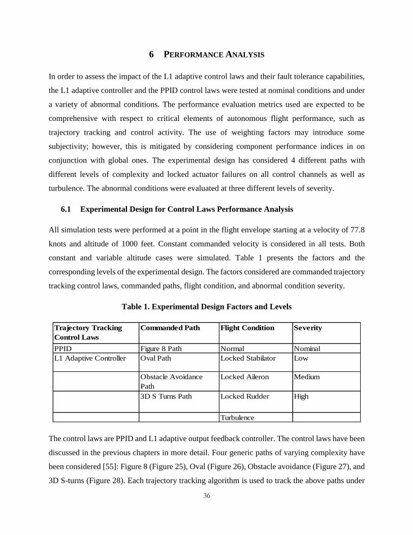
6.1 Experimental Design for Control Laws Performance Analysis
All simulation tests were performed at a point in the flight envelope starting at a velocity of 77.8
knots and altitude of 1000 feet. Constant commanded velocity is considered in all tests. Both
constant and variable altitude cases were simulated. Table 1 presents the factors and the
corresponding levels of the experimental design. The factors considered are commanded trajectory
tracking control laws, commanded paths, flight condition, and abnormal condition severity.
Table 1. Experimental Design Factors and Levels
The control laws are PPID and L1 adaptive output feedback controller. The control laws have been
discussed in the previous chapters in more detail. Four generic paths of varying complexity have
been considered [55]: Figure 8 (Figure 25), Oval (Figure 26), Obstacle avoidance (Figure 27), and
3D S-turns (Figure 28). Each trajectory tracking algorithm is used to track the above paths under
Trajectory Tracking
Control Laws
Commanded Path Flight Condition Severity
PPID Figure 8 Path Normal Nominal
L1 Adaptive Controller Oval Path Locked Stabilator Low
Obstacle Avoidance
Path
Locked Aileron Medium
3D S Turns Path Locked Rudder High
Turbulence

37
normal and abnormal conditions. The flight conditions include nominal, locked aerodynamic
surface (stabilator, aileron, or rudder) and atmospheric turbulence. Since the aircraft is symmetric
about the vertical plane of the body axes, locked right aerodynamic surface is assumed equivalent
to locked left surface. In this thesis, only the locked right surface case is considered, without any
loss of generality.
Figure 25. Figure 8 Path [55]

38
Figure 26. Oval Path [55]
Figure 27. Obstacle Avoidance Path [55]

39
Figure 28. 3D S-Turns Path [55]
The lockage of the aerodynamic surface occurs after 5 seconds into the simulation. The
performance of the controller was evaluated at three different levels of severity of the abnormal
conditions as presented in Table 2. The severity levels of the failure are low, medium, and high.
The corresponding deflection values vary from 2 degrees to 8 degrees. The standard deviation of
relative air velocity due to turbulence varies between 5 and 15 ft/sec.
Table 2. Description of Abnormal Condition Severities
The outcomes of the experiments include all system states and inputs necessary to calculate the
performance evaluation metrics as described in Section 6.2.
Stabilator Aileron Rudder Turbulence
(degrees) (degrees) (degrees) (ft/sec)
Low 2 2 2 5
Medium 5 5 5 10
Severe 8 8 8 15
Severity

40
6.2 Performance Evaluation Metrics
The overall performance of a controller is defined using two primary performance criteria [55].
The first criterion is based on the trajectory tracking accuracy with minimum errors on individual
axes and globally. The second criterion is based on the amount of control actuation. The control
activity indices assess performance in terms of the controller’s ability to keep track of the trajectory
with minimum control surface excursions and without reaching saturation.
6.2.1 Trajectory Tracking Indices
The trajectory tracking performance is evaluated using maximum, mean, and standard deviation
of the trajectory tracking errors in the horizontal XY plane, along the vertical Z-axis, and in the 3-
D physical space. This results in a total of 9 indices. Let x(t), y(t), and z(t) be the commanded
trajectory point at time t and 𝑥𝑎(𝑡), 𝑦𝑎(𝑡), and 𝑧𝑎(𝑡) the actual aircraft position at the same time.
First, the three tracking errors are defined as:
𝑥𝑦𝑒𝑟𝑟𝑜𝑟 = √[𝑥𝑎(𝑡) − 𝑥(𝑡)]2 + [𝑦𝑎(𝑡) − 𝑦(𝑡)]2 (35)
𝑧𝑒𝑟𝑟𝑜𝑟 = √[𝑧𝑎(𝑡) − 𝑧(𝑡)]2 (36)
𝑥𝑦𝑧𝑒𝑟𝑟𝑜𝑟 = √[𝑥𝑎(𝑡) − 𝑥(𝑡)]2 + [𝑦𝑎(𝑡) − 𝑦(𝑡)]2 + [𝑧𝑎(𝑡) − 𝑧(𝑡)]2 (37)
Then, for the total simulation time or for a pre-defined length of time, all the nine trajectory
tracking indices can be defined as follows.
The maximum tracking error is:
𝑥𝑦𝑚𝑎𝑥 𝑒𝑟𝑟𝑜𝑟 = 𝑚𝑎𝑥 (|𝑥𝑦𝑒𝑟𝑟𝑜𝑟|) (38)
𝑧𝑚𝑎𝑥𝑒𝑟𝑟𝑜𝑟 = 𝑚𝑎𝑥 (|𝑧𝑒𝑟𝑟𝑜𝑟|) (39)
𝑥𝑦𝑧𝑚𝑎𝑥 𝑒𝑟𝑟𝑜𝑟 = 𝑚𝑎𝑥 (|𝑥𝑦𝑧𝑒𝑟𝑟𝑜𝑟|) (40)
The average tracking error is:
𝑥𝑦𝐴𝑣𝑒𝑒𝑟𝑟𝑜𝑟 = 𝑚𝑒𝑎𝑛 (|𝑥𝑦𝑒𝑟𝑟𝑜𝑟|) (41)

41
𝑧𝐴𝑣𝑒𝑒𝑟𝑟𝑜𝑟 = 𝑚𝑒𝑎𝑛 (|𝑧𝑒𝑟𝑟𝑜𝑟|) (42)
𝑥𝑦𝑧𝐴𝑣𝑒𝑒𝑟𝑟𝑜𝑟 = 𝑚𝑒𝑎𝑛 (|𝑥𝑦𝑧𝑒𝑟𝑟𝑜𝑟|) (43)
The standard deviation of the tracking error is:
𝑥𝑦𝑒𝑟𝑟𝑜𝑟𝑆𝑡𝑑 = 𝑠𝑡𝑑(𝑥𝑦𝑒𝑟𝑟𝑜𝑟) (44)
𝑧𝑒𝑟𝑟𝑜𝑟𝑆𝑡𝑑 = 𝑠𝑡𝑑(𝑧𝑒𝑟𝑟𝑜𝑟) (45)
𝑥𝑦𝑧𝑒𝑟𝑟𝑜𝑟𝑆𝑡𝑑 = 𝑠𝑡𝑑(𝑥𝑦𝑧𝑒𝑟𝑟𝑜𝑟) (46)
6.2.2 Control Activity Indices
The control activity indices are defined using two important parameters: the integral of the absolute
value of the rate of change of actuator deflection, and the actuator saturation percentage. Therefore,
a total of 8 indices result for the 4 actuators considered: stabilator, aileron, rudder, and throttle.
Let 𝛿𝑎, 𝛿𝑒, 𝛿𝑟, and 𝛿𝑡 be the actual deflections of the stabilator, aileron, rudder, and throttle,
respectively; then the control activity indices are defined as follows [55].
Denoting the total test duration by T, the integral of aileron, stabilator, rudder deflection and
throttle rate of change is:
𝐼�̇�𝑎
= 1
𝑇∫ |�̇�𝑎(𝑡)|
𝑇
0
𝑑𝑡 (47)
𝐼�̇�𝑒
= 1
𝑇∫ |�̇�𝑒(𝑡)|
𝑇
0
𝑑𝑡 (48)
𝐼�̇�𝒓
= 1
𝑇∫ |�̇�𝑟(𝑡)|
𝑇
0
𝑑𝑡 (49)
𝐼�̇�𝑡
= 1
𝑇∫ |�̇�𝑡(𝑡)|
𝑇
0
𝑑𝑡 (50)
The stabilator saturation index assuming non-symmetric positive and negative extreme deflections
is defined as:

42
𝑆𝛿𝑒 =
100
𝑇∫ (𝛿𝑒1(𝑡)
𝑇
0
+ 𝛿𝑒2(𝑡))𝑑𝑡 (51)
where 𝛿𝑒1 = {0 𝑓𝑜𝑟𝛿𝑒 < 𝛿𝑒𝑚𝑎𝑥
1 𝑓𝑜𝑟𝛿𝑒 ≥ 𝛿𝑒𝑚𝑎𝑥 𝛿𝑒2 = {
0 𝑓𝑜𝑟𝛿𝑒 > 𝛿𝑒𝑚𝑖𝑛
1 𝑓𝑜𝑟𝛿𝑒 ≤ 𝛿𝑒𝑚𝑖𝑛
The aileron saturation index with symmetric extreme deflections is defined as:
𝑆𝛿𝑎 =
100
𝑇∫ 𝛿𝑎(𝑡)𝑑𝑡
𝑇
0
(52)
where 𝛿𝑎 = {0 𝑓𝑜𝑟|𝛿𝑎| < 𝛿𝑎𝑚𝑎𝑥
1 𝑓𝑜𝑟|𝛿𝑎| ≥ 𝛿𝑎𝑚𝑎𝑥
The rudder saturation index is defined as:
𝑆𝛿𝑟 =
100
𝑇∫ 𝛿𝑟(𝑡)𝑑𝑡
𝑇
0
(53)
where 𝛿𝑟 = {0 𝑓𝑜𝑟|𝛿𝑟| < 𝛿𝑟𝑚𝑎𝑥
1 𝑓𝑜𝑟|𝛿𝑟| ≥ 𝛿𝑟𝑚𝑎𝑥
The throttle saturation index is defined as:
𝑆𝛿𝑡 =
100
𝑇∫ 𝛿𝑡(𝑡)𝑑𝑡
𝑇
0
(54)
where 𝛿𝑡 = {0 𝑓𝑜𝑟𝛿𝑡 < 𝛿𝑡𝑚𝑎𝑥
1 𝑓𝑜𝑟𝛿𝑡 ≥ 𝛿𝑡𝑚𝑎𝑥
6.2.3 Total Performance Index (PI)
To analyze the performance of the different controllers, all trajectory tracking indices and control
activity indices are considered. A normalization and weighted sum process applied to the 17
individual indices is used to obtain one overall PI. The normalization values for each of the 17
indices were chosen based on the performance of all the controllers, while the weights of each
index were chosen based on the importance of that index towards the total performance index
(Table 3).

43
Table 3. Performance Index Weights and Normalization Cut-offs [55]
A total trajectory tracking index (TTI) is computed based on the 9 individual indices pertinent to
trajectory tracking performance. TTI takes values between 1 and 0. TTI values close to 1 indicate
the trajectory tracking is achieved with minimal error, whereas TTI close to 0 indicates that the
controller produces large tracking errors leading to loss of control and/or crash. A similar approach
is applied to the total control activity index (CAI), which is obtained as a weighted sum of the 8
individual indices pertinent to control usage. CAI values close to 1 indicate that the controller is
achieving the task with a small amount of control actuator activity without reaching the extreme
deflections, whereas values close to 0 indicate that the controller is commanding large control
activity, possibly with saturation. The total performance index (PI) was calculated using the
constant weight method for the total length of the path. A set of constant weights was selected to
sum the overall trajectory tracking and the overall control activity index into the total performance
index. The set of weights used were 0.7 for the trajectory tracking index and 0.3 for the control
activity index, which is considered to be a typical distribution adequate for numerous tasks and
missions [55]. For the given weights, PI above 0.6 generally provides “good” tracking with little
deviation from the commanded path and limited control actuation. Performance indices in the
range of 0.3 to 0.6 typically provide worse tracking with intensive control actuation and some
saturation. Performance indices below 0.3 are generally obtained when the tracking errors are very
large despite excessive control activity. In many of these situations, the aircraft cannot complete
the entire mission.
Global PI Weight
XY Z XYZ XY Z XYZ XY Z XYZ
Normalization Cut-off 50 50 50 10 10 10 5 5 5
0.06 0.08 0.06 0.12 0.16 0.12 0.12 0.16 0.12
0.7
Elevator Aileron Rudder Throttle Elevator Aileron Rudder Throttle
Normalization Cut-off 0.5 0.5 0.5 20 100 100 100 100
0.1 0.1 0.1 0.2 0.1 0.1 0.1 0.2
0.3
Surface Activation Index Saturation Index
Max Mean Standard Deviation
Control Activity Performance
Trajectory Tracking Performance
TTw
TTw
CAw
CAw

44
6.3 Results
Extensive flight simulation tests have been performed for all four paths and the results obtained
are discussed in this section. Complete result tables are included in Appendices A, B, C, and D for
figure 8 path, 3D s-turns, oval path, and OA path, respectively.
Tables A1, B1, C1, and D1 present the maximum tracking error values achieved with the PPID
control laws and the PPID augmented with the L1 adaptive output feedback controller for all four
paths, respectively. Tracking error values are computed along the vertical axis Z, in the horizontal
plane XY, and in three dimensions, XYZ, under nominal conditions, aileron failures, stabilator
failures, and rudder failures. Results under turbulence of different intensity are also included.
For figure 8 path, in all cases considered, the L1 augmentation consistently reduces the values of
the maximum tracking errors. The relative reduction is more significant on the vertical channel. It
should be noted that the L1 augmentation can handle the more demanding cases when PPID alone
cannot provide adequate compensation, such as the locked aileron and rudder at 8 degrees. In
particular, under rudder failure, the maximum tracking error with PPID is 478 m, while the error
with L1 is 14.3 m, which is close to the value of 13.8 m recorded for nominal flight. It can be
noticed that in terms of maximum tracking error, the L1 control laws are more robust with respect
to abnormal conditions maintaining the values reached under nominal conditions.
The superior robustness of the L1 control laws as compared to PPID can be noticed for the 3-D s-
turns as well. However, at nominal conditions and under mild failure conditions, the non-adaptive
control laws achieve lower maximum tracking errors. For example, for the PPID control laws, the
maximum tracking error is 26.6. m at nominal conditions, 28.9 for aileron stuck at 2 degrees, 35.7
m for aileron stuck at 5 degrees, and 849 m for aileron stuck at 8 degrees. The L1 control laws
maintain a value of 35.4 m for all these cases. This makes the 3-D s-turns path the most demanding
in terms of this performance parameter.
The same trends observed for the figure 8 path are present for the oval path, with the exception of
stabilator failure cases, where the values of the maximum tracking errors for the two sets of control
laws are very close to each other. It should be noted that the oval path appears to be less demanding
and the values of the maximum error vary less with the severity of the abnormal condition.
45
However, a maximum error of 49 m is reached by the PPID under aileron failure, while the L1
controller maintains a value of 16 m.
The OA path is the second most demanding task. L1 control laws achieve a maximum tracking
error around 20 m for all cases considered exhibiting the same robustness with respect to abnormal
conditions as previously noted. Control is lost with PPID under aileron stuck at 8 degrees;
however, with L1 the tracking performance is maintained close to nominal conditions.
Tables A2, B2, C2, and D2 present the mean of the tracking error values achieved with the PPID
control laws and the PPID augmented with the L1 adaptive output feedback controller for all four
paths, respectively. Tracking error values are computed along the vertical axis Z, in the horizontal
plane XY, and in three dimensions, XYZ, under nominal conditions, aileron failures, stabilator
failures, and rudder failures. Results under turbulence of different intensity are also included.
Tables A3, B3, C3, and D3 present corresponding values of the standard deviation of the tracking
errors.
For all four paths, the trends recorded for the maximum tracking errors are also present for the
mean and the standard deviation of the tracking errors. The ranking of the four paths with respect
to the mean tracking errors is preserved, with the 3-D s-turns being the most demanding, followed
in order by the OA, oval, and figure 8 paths. In terms of standard deviation, the largest values are
recorded for the 3-D s-turns, followed by the oval, OA, and figure 8 paths.
The controller activity index is comprised of two parameters: integral of control surface deflection
rate and saturation index. These two parameters should be minimum in order to attend the
maximum controller activity index. It should be noted that the maximum controller activity can be
simply achieved by not activating any of the control surfaces, which might result in very poor
tracking or even the crash of the aircraft. Therefore, these metrics should be considered in
conjunction with the tracking performance such that better trajectory tracking is achieved with
limited and gradual changes in the control surface deflections.
Tables A4, B4, C4, and D4 present the integral of control actuation rate achieved with the PPID
control laws and the PPID augmented with the L1 adaptive output feedback controller for all four
paths, respectively. These tables include the integrals of control surface deflection rates for
stabilator, aileron, and rudder as well as the integral of throttle rate. From the tables, it can be

46
noticed that the deflection rates of stabilator and aileron for L1 adaptive controller are not as
gradual as the PPID controller, whereas the deflection rates of rudder and throttle for L1 adaptive
controller are more gradual than the PPID controller under nominal and all abnormal conditions.
The result of high aileron and stabilator deflection rates of L1 adaptive controller is the superior
trajectory tracking. L1 adaptive controller tracks better than PPID with a slight increase in the
deflection rates. The same trends observed for the figure 8 path are present for the oval path and
OA path. The most demanding case is 3D S Turns. The deflection rates of L1 adaptive controller
show more gradual changes than the PPID. The PPID poorly tracks the trajectory with great strain
in the control activity.
The values of the saturation index for the four actuators over the four paths are presented in Tables
A5, B5, C5, and D5, respectively. The aileron saturation index of L1 adaptive over the figure 8
path is slightly larger than the PPID controller for all levels of aileron failures, medium stabilator
failures, severe stabilator failures, and severe rudder failures. The throttle saturation index for
severe aileron and rudder failures of PPID controller is slightly larger than the L1 adaptive
controller. The same trends observed for the figure 8 path are present for the oval path with the
exception of throttle saturation index, which is zero for both sets of control laws. The results for
the OA path have similar trends as for the oval path. The L1 can handle better throttle saturation
for severe aileron failure than the PPID controller. The performance of L1 adaptive controller is
dominant in the 3D S Turns path. The L1 adaptive controller performs better than the PPID
controller in terms of this metric for all aileron and rudder failures, as well as under turbulence
conditions.
The values of the composite TTI, CAI, and PI are listed in Tables A6, B6, C6, and D6, for the four
paths, respectively.
The results for figure 8 shown in Table A6, lead to the conclusion that the L1 adaptive controller
handles better the trajectory tracking than PPID controller under all conditions and the
performance of L1 adaptive controller is dominant for the severe aileron and rudder failures. The
controller activity performance of L1 adaptive controller is almost equal or slightly less than PPID
controller for all conditions except for the values of severe rudder failure. Therefore, the L1
adaptive controller performs better trajectory tracking with less controller activity as compared to
47
the PPID controller for all abnormal conditions. The L1 adaptive controller performance index is
twice the PPID index for the severe aileron and rudder failures.
The trends for figure 8 path are the same as for the oval and OA path. The only difference is that
the PPID controller loses control for severe aileron failures. The most demanding path is 3D S
Turns. The L1 adaptive controller tracks better the trajectory with minimal controller activity for
all cases. The PPID performance is poor for the severe aileron failure.
Table 4 shows the percentage increase of the TTI of L1 adaptive controller over PPID controller
for all four paths. The percentage increase is calculated using the formula:
% 𝑖𝑛𝑐𝑟𝑒𝑎𝑠𝑒 = 𝑇𝑇𝐼 𝑜𝑓 𝐿1 𝑎𝑑𝑎𝑝𝑡𝑖𝑣𝑒 𝑐𝑜𝑛𝑡𝑟𝑜𝑙𝑙𝑒𝑟 − 𝑇𝑇𝐼 𝑜𝑓 𝑃𝑃𝐼𝐷 𝑐𝑜𝑛𝑡𝑟𝑜𝑙𝑙𝑒𝑟
𝑇𝑇𝐼 𝑜𝑓 𝑃𝑃𝐼𝐷 𝑐𝑜𝑛𝑡𝑟𝑜𝑙𝑙𝑒𝑟𝑥100
Figure 29, Figure 30, Figure 31 and Figure 32 present the TTI of PPID and the L1 adaptive
controller for figure 8 path, oval path, OA path and 3D S-Turns path, respectively. From the Figure
29, the L1 adaptive controller has a better trajectory tracking performance index than PPID under
nominal and all abnormal failures. It is observed that in all cases, the percentage increase of TTI
of L1 adaptive controller over PPID is 1 to 3 %. In particular, the percentage increase of L1
adaptive controller over PPID for severe aileron and severe rudder failure is 125% and 115%
respectively. Figure 30, Figure 31 show similar trends with drastic percentage increase of 57.197%
and 113.990% respectively for severe aileron failures. Figure 32 presents the L1 adaptive
controller having a better trajectory tracking performance index than PPID under severe aileron
and rudder failures. It is also observed that the L1 adaptive controller performs better in adverse
conditions while PPID performs better in nominal condition. The percentage increase of L1 over
PPID under severe aileron and rudder failures are 81% and 12% respectively.

48
Table 4. Percentage Increase of TTI for all Four Paths
TTI
Percentage increase of L1 adaptive controller over PPID
Figure 8 Oval OA 3D S Turns
Nominal 1.529 1.467 1.728 -11.31
Aileron stuck at 2 deg 2.370 1.467 2.101 -8.587
Aileron stuck at 5 deg 3.721 1.096 2.481 -1.049
Aileron stuck at 8 deg 125.0 57.20 114.0 81.04
Stab stuck at 2 deg 2.387 1.220 2.112 1.389
Stab stuck at 5 deg 3.281 1.225 2.125 2.028
Stab stuck at 8 deg 4.461 1.111 3.042 12.35
Rudder stuck at 2 deg 0.815 1.605 1.487 -12.20
Rudder stuck at 5 deg 0.579 2.642 1.619 -12.06
Rudder stuck at 8 deg 115.4 6.525 2.919 -6.553
Light Turbulence 1.410 1.834 1.726 -11.38
Moderate Turbulence 1.178 1.838 14.53 -11.57
Severe Turbulence 1.070 1.854 -4.075 -11.05

49
Figure 29. Trajectory Tracking Performance Index of PPID and L1 Adaptive Controller
for Figure 8 Path
Figure 30. Trajectory Tracking Performance Index of PPID and L1 Adaptive Controller
for Oval Path
0
0.1
0.2
0.3
0.4
0.5
0.6
0.7
0.8
0.9
1
PPID
L1+PPID

50
Figure 31. Trajectory Tracking Performance Index of PPID and L1 Adaptive Controller
for OA Path
Figure 32. Trajectory Tracking Performance Index of PPID and L1 Adaptive Controller
for 3D S Turns Path

51
Table 5 shows the percentage increase of the CAI of L1 adaptive controller over PPID controller
for all four paths. Figure 33, Figure 34, Figure 35, and Figure 36 show CAI of PPID controller and
L1 adaptive controller for figure 8 path, oval path, oa path and 3D S-Turns path, respectively.
From Figure 33, the performance index of CAI of L1 adaptive controller is almost equal or little
less than the PPID. The percentage increase of L1 adaptive controller over PPID for severe aileron
and severe rudder failures are 4.678% and 65.976% respectively. Figure 34 shows that L1 adaptive
control activity performance is equal or less than the PPID. Figure 35 shows that L1 adaptive
controller performs better than PPID for the severe aileron failure. In Figure 36, the CAI of L1
adaptive controller reaches almost twice the value for the PPID controller under nominal
conditions, turbulence, and failures of the aileron and rudder. In all mild, moderate, and severe
stabilator failure, the CAI of L1 adaptive controller is equal or less than the CAI of PPID controller.
Table 5. Percentage Increase of CAI for all Four Paths
CAI
Percentage increase of L1 adaptive controller over PPID
Figure 8 Oval OA 3D S Turns
Nominal 0.101 0.203 0.101 110.1
Aileron stuck at 2 deg -0.203 -0.305 -0.409 118.5
Aileron stuck at 5 deg 0.000 -0.306 -0.308 113.3
Aileron stuck at 8 deg 4.678 0.448 338.4 554.8
Stab stuck at 2 deg -0.303 -0.101 -0.406 -0.103
Stab stuck at 5 deg -0.810 0.000 -0.711 -1.241
Stab stuck at 8 deg -3.760 0.102 -1.531 -5.280
Rudder stuck at 2 deg 0.000 0.102 -0.203 117.8
Rudder stuck at 5 deg -0.101 -0.305 -0.406 117.2
Rudder stuck at 8 deg 65.98 -4.094 -1.427 115.8
Light Turbulence -1.019 -0.817 -1.745 107.1
Moderate Turbulence -2.174 -2.599 -1.563 101.7
Severe Turbulence -3.404 -3.419 -4.463 94.81

52
Figure 33. Controller Activity Performance Index of PPID and L1 Adaptive Controller for
Figure 8 Path
Figure 34. Controller Activity Performance Index of PPID and L1 Adaptive Controller for
Oval Path
0
0.2
0.4
0.6
0.8
1
1.2
PPID
L1+PPID
0
0.2
0.4
0.6
0.8
1
1.2
PPID
L1+PPID

53
Figure 35. Controller Activity Performance Index of PPID and L1 Adaptive Controller for
OA Path
Figure 36. Controller Activity Performance Index of PPID and L1 Adaptive Controller for
3D S Turns Path

54
Table 6 shows the percentage increase of L1 adaptive controller over PPID controller of the PI for
all four paths. Figure 37, Figure 38, Figure 39, and Figure 40 show the PI of PPID and the L1
adaptive controller for figure 8 path, oval, OA, and 3D S-Turns paths, respectively. From Figure
37, it is observed that in all cases the total performance index of L1 adaptive controller is better
than the PPID controller. In severe aileron and rudder failures, the PI of L1 adaptive controller is
twice the value reached with the PPID controller. The PI of L1 adaptive controller shows
significant improvement under nominal and turbulence conditions, as well as in the presence of
aileron and rudder failures. In the case of stabilator failures, the PI of L1 adaptive controller reaches
lower values that those obtained with the PPID control laws. Figure 38, and Figure 39 show the
same trends recorded for figure 8 path with a 155% increase of L1 adaptive controller performance
for the severe aileron failures. From Figure 40, it can be noticed that the PI of L1 is higher in all
cases. There is also noticeable increase of PI of L1 over PPID under turbulence conditions.
Table 6. Percentage Increase of PI for all Four Paths
PI
Percentage increase of L1 adaptive controller over PPID
Figure 8 Oval OA 3D S Turns
Nominal 1.009 1.159 1.159 14.39
Aileron stuck at 2 deg 1.467 1.281 1.281 17.87
Aileron stuck at 5 deg 2.509 1.519 1.519 24.54
Aileron stuck at 8 deg 66.29 155.3 155.3 146.4
Stab stuck at 2 deg 1.586 1.281 1.281 0.806
Stab stuck at 5 deg 1.833 1.168 1.168 0.677
Stab stuck at 8 deg 1.628 1.537 1.537 5.014
Rudder stuck at 2 deg 0.445 0.929 0.929 14.46
Rudder stuck at 5 deg 0.333 0.933 0.933 14.31
Rudder stuck at 8 deg 96.15 1.418 1.418 19.13
Light Turbulence 0.674 0.465 0.465 13.42
Moderate Turbulence 0.113 -0.117 -0.117 12.18
Severe Turbulence -0.459 -0.941 -0.941 10.83

55
Figure 37. Total Performance Index of PPID and L1 Adaptive Controller for Figure 8 Path
Figure 38. Total Performance Index of PPID and L1 Adaptive Controller for Oval Path
0
0.1
0.2
0.3
0.4
0.5
0.6
0.7
0.8
0.9
1
PPID
L1+PPID
0
0.1
0.2
0.3
0.4
0.5
0.6
0.7
0.8
0.9
1
PPID
L1+PPID
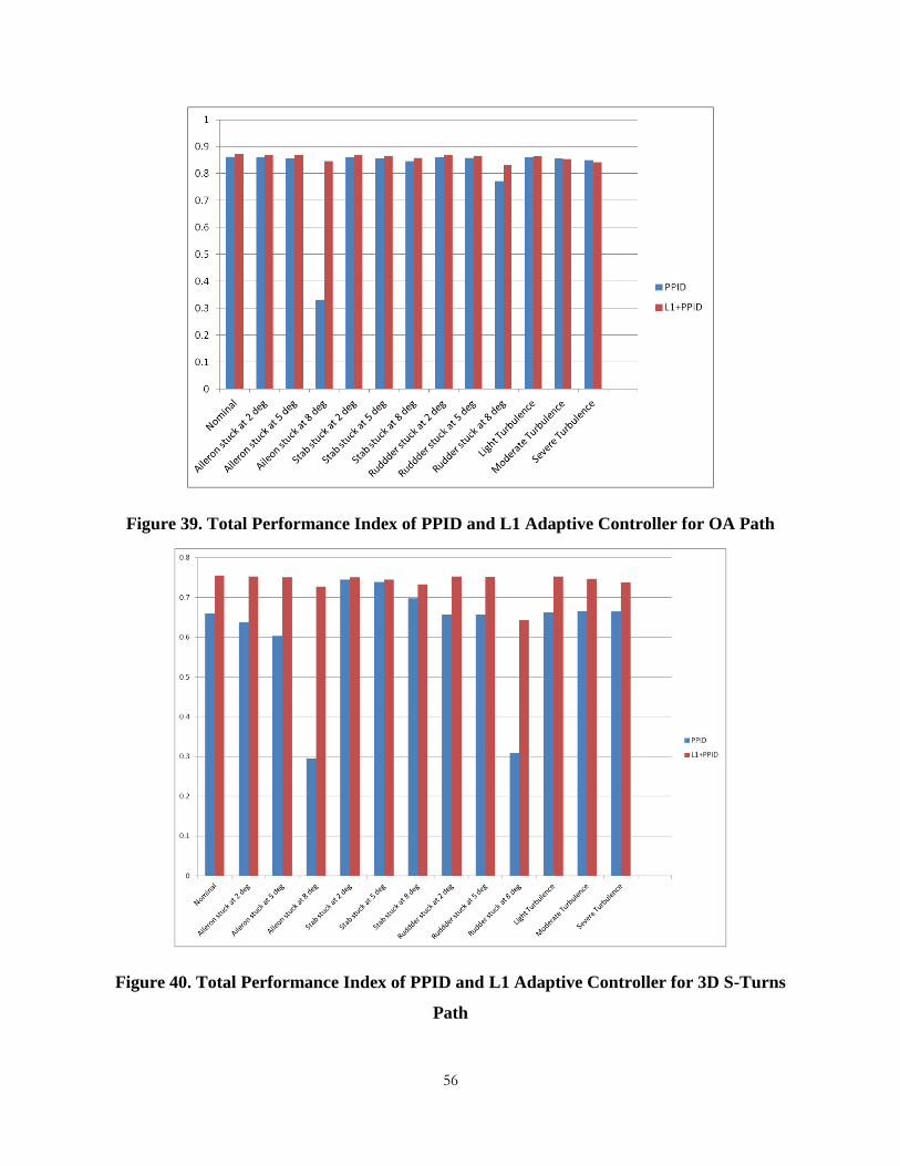
56
Figure 39. Total Performance Index of PPID and L1 Adaptive Controller for OA Path
Figure 40. Total Performance Index of PPID and L1 Adaptive Controller for 3D S-Turns
Path
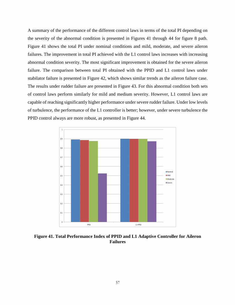
57
A summary of the performance of the different control laws in terms of the total PI depending on
the severity of the abnormal condition is presented in Figures 41 through 44 for figure 8 path.
Figure 41 shows the total PI under nominal conditions and mild, moderate, and severe aileron
failures. The improvement in total PI achieved with the L1 control laws increases with increasing
abnormal condition severity. The most significant improvement is obtained for the severe aileron
failure. The comparison between total PI obtained with the PPID and L1 control laws under
stabilator failure is presented in Figure 42, which shows similar trends as the aileron failure case.
The results under rudder failure are presented in Figure 43. For this abnormal condition both sets
of control laws perform similarly for mild and medium severity. However, L1 control laws are
capable of reaching significantly higher performance under severe rudder failure. Under low levels
of turbulence, the performance of the L1 controller is better; however, under severe turbulence the
PPID control always are more robust, as presented in Figure 44.
Figure 41. Total Performance Index of PPID and L1 Adaptive Controller for Aileron
Failures
0
0.1
0.2
0.3
0.4
0.5
0.6
0.7
0.8
0.9
1
PPID L1+PPID
Nominal
Mild
Moderate
Severe

58
Figure 42. Total Performance Index of PPID and L1 Adaptive Controller for Stabilator
Failures
Figure 43. Total Performance Index of PPID and L1 Adaptive Controller for Rudder
Failures
0.83
0.84
0.85
0.86
0.87
0.88
0.89
0.9
0.91
PPID L1+PPID
Nominal
Mild
Moderate
Severe
0
0.1
0.2
0.3
0.4
0.5
0.6
0.7
0.8
0.9
1
PPID L1+PPID
Nominal
Mild
Moderate
Severe

59
.
Figure 44. Total Performance Index of PPID andL1 Adaptive Controller under Turbulence
Conditions
The performance analysis is extended in finding the average of the severe failures over four paths
of the two controllers. That is the average of severe aileron failure of the four paths of PPID and
L1+PPID is calculated and shown as red bar in Figure 45. Similarly, the other severe failures and
nominal is calculated and presented below. The L1 adaptive controller tracks the path better than
PPID under nominal and all abnormal failures. The prominent increase in the total PI is for severe
aileron and severe rudder failures. From the figure, it is evident that L1 controller is capable of
handling the most adverse failures, whereas the performance of PPID is not that adequate to handle
complicated paths.
0.85
0.86
0.87
0.88
0.89
0.9
0.91
PPID L1+PPID
Nominal
Mild
Moderate
Severe
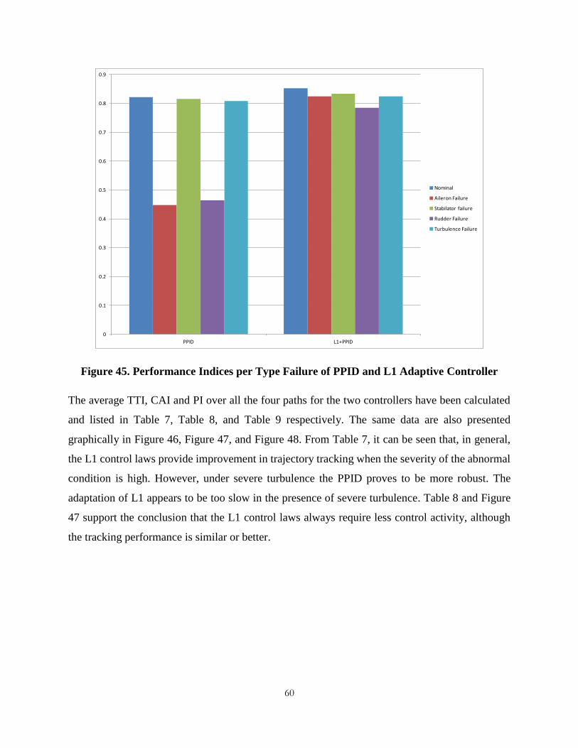
60
Figure 45. Performance Indices per Type Failure of PPID and L1 Adaptive Controller
The average TTI, CAI and PI over all the four paths for the two controllers have been calculated
and listed in Table 7, Table 8, and Table 9 respectively. The same data are also presented
graphically in Figure 46, Figure 47, and Figure 48. From Table 7, it can be seen that, in general,
the L1 control laws provide improvement in trajectory tracking when the severity of the abnormal
condition is high. However, under severe turbulence the PPID proves to be more robust. The
adaptation of L1 appears to be too slow in the presence of severe turbulence. Table 8 and Figure
47 support the conclusion that the L1 control laws always require less control activity, although
the tracking performance is similar or better.
0
0.1
0.2
0.3
0.4
0.5
0.6
0.7
0.8
0.9
PPID L1+PPID
Nominal
Aileron Failure
Stabilator failure
Rudder Failure
Turbulence Failure

61
Table 7. Average Trajectory Tracking Performance Index of Four Paths for PPID and L1
Adaptive Controller
Average PI TT PPID L1 +PPID % increase of L1 adaptive controller over PPID
Nominal 0.805 0.794 -1.366
Aileron stuck at 2 deg 0.798 0.795 -0.376
Aileron stuck at 5 deg 0.782 0.795 1.662
Aileron stuck at 8 deg 0.416 0.795 91.11
Stab stuck at 2 deg 0.778 0.792 1.799
Stab stuck at 5 deg 0.770 0.787 2.208
Stab stuck at 8 deg 0.747 0.783 4.819
Rudder stuck at 2 deg 0.806 0.791 -1.861
Rudder stuck at 5 deg 0.802 0.789 -1.621
Rudder stuck at 8 deg 0.656 0.773 17.84
Light Turbulence 0.807 0.796 -1.363
Moderate Turbulence 0.807 0.821 1.735
Severe Turbulence 0.827 0.803 -2.902
Figure 46. Average Trajectory Tracking Performance Index of Four Paths for PPID and
L1 Adaptive Controller
0
0.1
0.2
0.3
0.4
0.5
0.6
0.7
0.8
0.9
PPID
L1 +PPID

62
Table 8. Average Controller Activity Performance Index of Four Paths for PPID and L1
Adaptive Controller
Average PI CA PPID L1 +PPID % increase of L1 adaptive controller over PPID
Nominal 0.858 0.987 21.21
Aileron stuck at 2 deg 0.847 0.976 21.02
Aileron stuck at 5 deg 0.846 0.973 22.58
Aileron stuck at 8 deg 0.521 0.891 91.17
Stab stuck at 2 deg 0.983 0.980 20.55
Stab stuck at 5 deg 0.981 0.974 20.80
Stab stuck at 8 deg 0.977 0.952 20.98
Rudder stuck at 2 deg 0.853 0.985 20.99
Rudder stuck at 5 deg 0.852 0.981 21.01
Rudder stuck at 8 deg 0.743 0.952 39.84
Light Turbulence 0.850 0.966 18.71
Moderate Turbulence 0.838 0.941 16.00
Severe Turbulence 0.820 0.903 9.268
Figure 47. Average Controller Activity Performance Index of Four Paths for PPID and L1
Adaptive Controller
0
0.2
0.4
0.6
0.8
1
1.2
PPID
L1 +PPID

63
The results for the PI presented in Table 9 and Figure 48 where obtained with a 0.70/0.30 weight
of the tracking and control metrics, which is a typical selection for a large variety of UAV missions
and tasks. In Figure 49, the percentage increase of the total PI obtained with the L1 control laws
as compared to the PPID is presented. From these data, it can be concluded that the L1 adaptive
controller achieves better performance under all nominal and abnormal conditions investigated in
this study.
Table 9. Average Total Performance Index of Four Paths for PPID and L1 Adaptive
Controller
Total PI PPID L1 +PPID % increase of L1 adaptive controller over
PPID
Nominal 0.820 0.851 3.780
Aileron stuck at 2 deg 0.811 0.848 4.562
Aileron stuck at 5 deg 0.798 0.847 6.140
Aileron stuck at 8 deg 0.371 0.823 121.8
Stab stuck at 2 deg 0.836 0.847 1.316
Stab stuck at 5 deg 0.831 0.841 1.203
Stab stuck at 8 deg 0.813 0.831 2.214
Rudder stuck at 2 deg 0.820 0.848 3.415
Rudder stuck at 5 deg 0.818 0.846 3.423
Rudder stuck at 8 deg 0.689 0.831 20.61
Light Turbulence 0.818 0.844 3.178
Moderate Turbulence 0.815 0.835 2.454
Severe Turbulence 0.809 0.822 1.607
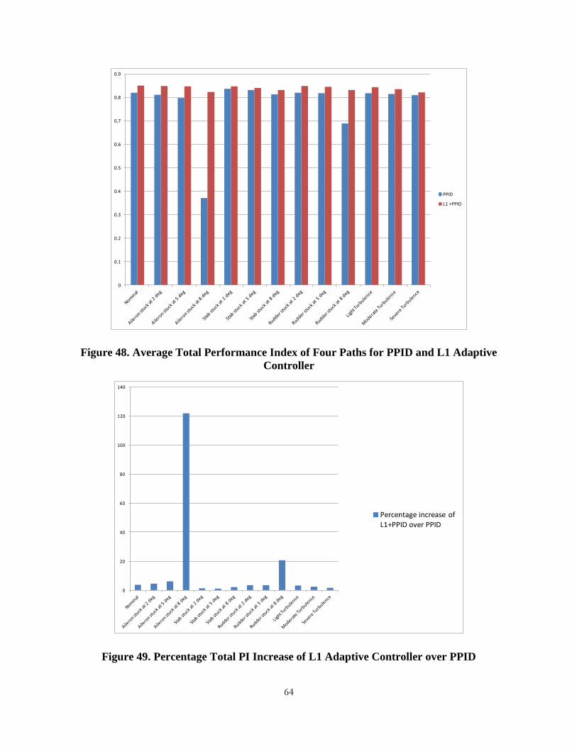
64
Figure 48. Average Total Performance Index of Four Paths for PPID and L1 Adaptive
Controller
Figure 49. Percentage Total PI Increase of L1 Adaptive Controller over PPID
0
0.1
0.2
0.3
0.4
0.5
0.6
0.7
0.8
0.9
PPID
L1 +PPID
0
20
40
60
80
100
120
140
Percentage increase of L1+PPID over PPID
65
7 CONCLUSION AND FUTURE WORK
In this thesis, the performance of an L1 augmentation of a baseline PPID controller for autonomous
flight was evaluated and analyzed. Four different commanded paths at normal and abnormal
conditions were considered. The abnormal conditions include turbulence and lockage of
aerodynamic control surfaces on the roll, pitch, and yaw channels. The evaluation was performed
in terms of composite evaluation indexes based on trajectory tracking and control activity.
The adaptive augmentation achieved generally better trajectory tracking performance under more
severe abnormal conditions. However, it exhibited less robustness to severe turbulence. In the 3D
S Turns path, the L1 control laws produced less control activity and less saturation.
The capability of the fault tolerant control laws to accommodate abnormal conditions is
conditioned by the complexity of the commanded trajectory and the nature and severity of the
abnormal condition.
The results of this study seem to support the idea that effective fault tolerant control laws should
be accompanied by powerful abnormal condition detection, identification, and evaluation schemes
that could adjust the nature and level of accommodation on a case by case basis.
All factors considered, shape of commanded paths, type of abnormal conditions and level of
severity have an impact on the relative ranking of the two control systems.
This study should be extended to include abnormal conditions of different nature affecting other
aircraft subsystems such as sensors, including GPS, structure, or propulsion system. The findings
obtained through simulation should be confirmed through actual flight tests.

66
BIBLIOGRAPHY
[1] Chao H., Cao Y., Chen Y. "Autopilots for Small Unmanned Aerial Vehicles: A Survey."
International Journal of Control, Automation and Systems 8.1 2010: 36-44. Print.
[2] Nayyerloo M., Chen X., Wang W., Geoffrey J. "Cable-Climbing Robots for Power
Transmission Lines Inspection." Mobile Robots - State of the Art in Land, Sea, Air, and
Collaborative Missions.” Vienna: I-Tech Education, 2009. 63-84. Print.
[3] Puri A.; Valavanis K.P., Kontitsis M., "Statistical profile generation for traffic monitoring
using real-time UAV based video data. "Control & Automation, 2007. MED '07.
Mediterranean Conference. vol., no., pp.1,6, 27-29 June 2007.
[4] Martínez-de-Dios J. R., Merino L., Ollero A., Ribeiro L.M., Viegas X., "Multi-UAV
Experiments: Application to Forest Fires." Multiple Heterogeneous Unmanned Aerial
Vehicles. Vol. 37. Berlin: Springer Berlin Heidelberg 2007. 207 - 228. Print.
[5] Mejias, L.; Campoy, P.; Saripalli, S.; Sukhatme, G. "A visual surveying approach for
tracking features in urban areas using an autonomous helicopter."Robotics and Automation.
2006. ICRA 2006. Proceedings 2006 IEEE International Conference. vol., no., pp.2503,
2508. 15-19 May 2006
[6] Marshall M., Neff J., Lao N., Yuhas P. Proc. of AIAA Defense and Civil Space Programs
Conference and Exhibit. The Aerospace Corporation. Los Angeles. CA. N.p.: American
Institute of Aeronautics and Astronautics. 1998. Print.
[7] Mejias L., Correa J.F., Mondragon I., Campoy P. "COLIBRI: A vision-Guided UAV for
Surveillance and Visual Inspection." Robotics and Automation, 2007 IEEE International
Conference. vol., no., pp.2760, 2761. 10-14 April 2007.
[8] Iñigo-Blasco P., Diaz-Del-Rio F., Romero-Ternero M.C., Cagigas-Muñiz D, Vicente-Diaz.
S. "Robotics Software Frameworks for Multi-agent Robotic Systems Development."
Robotics and Autonomous Systems 60.6 2012: 803-21. Print.
[9] Lee, D., Jae-Wook Yoo., Kang-Hee L., Yoon K. "A Real Time Flame and Smoke Detection
Algorithm Based on Conditional Test in YCbCr Color Model and Adaptive Differential

67
Image." Journal of the Korea Society of Computer and Information 15.5 (2010): 57-65.
Print.
[10] Gupta, S G., Mangesh M. G., Dr. Jawandhiya P M. "Review of Unmanned Aircraft System
(UAS)." International Journal of Advanced Research in Computer Engineering &
Technology (IJARCET) 2.4 2013: 1646-658. Print.
[11] Department of Defense. Unmanned Aircraft Systems Roadmap. Washington DC Army
Regulation 385-40. 2005.
[12] Cummings M. L., da Silva F B., Scott S D.,”Design Methodology for Unmanned Aerial
Vehicle (UAV) Team Coordination.” MIT Humans and Automation Laboratory.2007.
[13] Shima T., Rasmussen S.J., Sparks A G., "UAV cooperative multiple task assignments
using genetic algorithms."American Control Conference. 2005. Proceedings of the 2005.
vol., no., pp.2989.2994 vol. 5. 8-10 June 2005
[14] Wang J., Vijay V P., Chengyu C., Hovakimyan N., "Novel L1 Adaptive Control
Methodology for Aerial Refueling with Guaranteed Transient Performance." Journal of
Guidance, Control, and Dynamics 31.1 2008 182-93. Print.
[15] "Accident Threat Categories." Lessons Learned. 7 Apr. 2011. Web. accessed Jan,2014.
[16] "ECFR — Code of Federal Regulations." ECFR — Code of Federal Regulations. 1 Dec.
2011. Web. accessed Jan,2014.
[17] King, David W., Bertapelle, A., Moses, C., "UAV failure rate criteria for equivalent level
of safety." International Helicopter Safety Symposium, Montreal Quebec. Canada.
September 26-29, 2005.
[18] "Causes of Fatal Accidents by Decade." Accident Statistics. 1 Jan. 2012. Web. accessed
Jan,2014
[19] Department of the Army. Accident reporting and records. Washington. DC. Reference
no.14-S-0553. 1994a.

68
[20] Karas O., "UAV Simulation Environment for Autonomous Flight Control Algorithms."
Order No. 1520729 West Virginia University, 2012. Ann Arbor:“ProQuest.”Web. 9 Aug.
2014.
[21] Perhinschi M., Wilburn B., Wilburn J., Moncayo H., Karas O. "Simulation Environment
for UAV Fault Tolerant Autonomous Control Laws Development." Journal of Modeling,
Simulation, Identification, and Control 1.4. 2013: 164-95. Print.
[22] Newcome L.R., “Unmanned Aviation: A brief history of UAV’s. American Institute of
Aeronautics and Astronautics.” Reston 2004.
[23] Zaloga, S., Ian P., Unmanned Aerial Vehicles: Robotic Air Warfare. 1917-2007. Vol. 144.
Oxford: Osprey. 2008. Print.
[24] Dalamagkidis K., Valavanis KimonP., Dr. Piegl LesA."Aviation History and Unmanned
Flight." On Integrating Unmanned Aircraft Systems into the National Airspace System.
Vol. 54. Springer Netherlands. 2012. 11-42. Print.
[25] Maj. Jones A. C., “Unmanned Aerial Vehicles (UAVS) an Assessment of Historical
Operations and Future Possibilities”, Research Department Air Command and Staff
College. AU/ACSC/0230D/97-03. March 1997.
[26] Gertler J., “U.S. Unmanned Aerial Systems”. Congressional Research Service 7-
5700.R42136. January 3. 2012
[27] Jaysen A. Y. “The Vulnerabilities of Unmanned Aircraft System Common Data Links to
Electronic Attack".Master of Military Art and Science. U.S. Army. 1998.
[28] DoD. Unmanned Aircraft Systems Roadmap 2005-2030. Office of the Secretary of
Defense, Department of Defense, Washington, DC. August 2005.
[29] Helios Solar-Powered UAV Crashes - AVweb flash Article. Web.5 Sep. 2014.
<http://www.avweb.com/avwebflash/briefs/185240-1.html?redirected=1>
[30] Air Combat Command. MQ-1B PREDATOR ACCIDENT REPORT RELEASED. Web. 5
Sep. 2014. <http://www.acc.af.mil/news/story.asp?id=123332108>.

69
[31] X-51A Waverider spins out of control and crashes into after 15 seconds as $300M
hypersonic jet program FAILS latest test. Web.5 Sep. 2014.
<http://www.dailymail.co.uk/sciencetech/article-2188936/X-51-Waverider-spins-control-
crashes-ocean-15-seconds.html>.
[32] U.S. Navy 2012 Maryland Drone Crash Investigation Report Public Intelligence, 2013.
Web.5 Sep. 2014. <https://publicintelligence.net/usnavy-maryland-drone-crash-report/>.
[33] Johnson, Chris W., Shea C., “The Hidden Human Factors in Unmanned Aerial Vehicles.”
2008. Print.
[34] Department of Defense. Unmanned Aerial Vehicle Reliability Study. Washington. DC.
Feb. 2003.
[35] Tekinalp O., Isik S., Yavrucuk I., “Fault Tolerant Control of an Over Actuated UAV.”
AIAA Guidance, Navigation, and Control Conference. Oregon. Portland. N.p. AIAA.
2011. Print.
[36] Kaminer I., Pascoal A., Hallberg A.M., Silvestre C. "Trajectory Tracking for Autonomous
Vehicles: An Integrated Approach to Guidance and Control." Journal of Guidance,
Control, and Dynamics. Vol. 21. No. 1. 1998. pp. 29-38.
[37] Alvis W., Castillo C., Castillo E M., Moreno K., Valavanis K P., "A Tutorial Approach to
Small Unmanned Helicopter Controller Design for Non-Aggressive Flights." Advances in
Unmanned Aerial Vehicles - State of the Art and the Road to Autonomy. edited by
Valavanis. K. P., Vol. 33. Springer. Norwell. MA, 2007. pp. 119-170.
[38] Beard R., McLain T. “Small Unmanned Aircraft: Theory and Practice.” Princeton. NJ:
Princeton University Press. 2012.
[39] Pfeifer E., Kassab F. "Dynamic Feedback Controller of an Unmanned Aerial
Vehicle,"Robotics Symposium and Latin American Robotics Symposium (SBR-LARS).
2012 Brazilian. vol., no., pp.261.266. 16-19 Oct. 2012.
[40] Sung K H., Yoonsu N. “Stable fuzzy control system design with pole-placement constraint:
an LMI approach.” Computers in Industry. Volume 51. Issue 1. May 2003. Pages 1-11.

70
[41] Chilali M., Gahinet P., "H∞ design with pole placement constraints: an LMI approach."
Automatic Control. IEEE Transactions. vol.41. no.3. pp.358,367. Mar 1996.
[42] Kinoshita T., Imado F., "A Study on the Optimal Flight Control for an Autonomous
UAV."Mechatronics Automation, Proceedings of the 2006 IEEE International
Conference. vol., no., pp.996.1001. 25-28 June 2006.
[43] S. Franko, “LQR-Based Trajectory Control Of Full Envelope, Autonomous Helicopter,”
Proceedings of the World Congress on Engineering 2009, London, 1-3, July 2009.
[44] Oner K T., Ertugrul C., Efe S., Cevdet H., Taylan A., Mustafa U. "LQR and SMC
Stabilization of a New Unmanned Aerial Vehicle." World Academy of Science,
Engineering & Technology 34 2009: 373-78. Print.
[45] Masar, I., E. Stohr, “Gain-scheduled LQR-control for an Autonomous Airship.” Proc. of
18th International Conference on Process Control. Slovakia. Tatranská Lomnica. N.p. n.p.
2011. 197-204. Print.
[46] Hajiyev C., Vural S. "LQR Controller with Kalman Estimator Applied to UAV
Longitudinal Dynamics,"Positioning. Vol. 4 No. 1, 2013, pp. 36-41.doi:10.4236
/pos.2013.41005.
[47] Beard R., Kingston D., Quigley M., Snyder D., Christiansen R., Johnson W., McLain T.,
Goodrich M. A. "Autonomous Vehicle Technologies for Small Fixed-Wing UAVs." AIAA
Journal of Aerospace Computing, Information, and Communications. Vol. 2. No. 1. 2005.
pp. 92-108.
[48] Beard R., McLain T. Small Unmanned Aircraft: Theory and Practice. Princeton, NJ:
Princeton University Press. 2012.
[49] Kada B., Ghazzawi.Y. Robust PID Controller Design for an UAV Flight Control System.
Proc. of World Congress on Engineering and Computer Science 2011, USA, San
Francisco. Vol. II. N.p.: n.p., 2011. 945-50. Print.

71
[50] Perhinschi M. G., “A Modified Genetic Algorithm for the Design of Autonomous
Helicopter Control System.” Proceedings of the AIAA Guidance, Navigation and Control
Conference. New Orleans LA, USA. August 1997. pp. 1111-1120
[51] Salih A L., Moghavvemi M., Mohamed H A F., Gaeid K S. "Flight PID Controller Design
for a UAV Quadrotor." Scientific Research and Essays 5.23 (2010): 3660-667. Print.
[52] Bouabdallah S., Noth A., Siegwart R., "PID vs LQ control techniques applied to an indoor
micro quadrotor."Intelligent Robots and Systems. 2004. (IROS 2004). Proceedings. 2004
IEEE/RSJ International Conference . vol.3. no., pp.2451.2456 vol.3. 28 Sept.-2 Oct. 2004.
[53] Jun L., Yuntang L., "Dynamic analysis and PID control for a quadrotor." Mechatronics
and Automation (ICMA), 2011 International Conference. vol., no., pp.573.578. 7-10 Aug.
2011
[54] Azinheira J. R., Paivab D. E. C., Ramos J G., Bueno S. S. "Mission Path Following for an
Autonomous Unmanned Airship," Proceedings of the 2000 IEEE International Conference
on Robotics and Automation. San Francisco. CA. April, 2000. pp. 1269-1275.
[55] Wilburn B., Perhinschi M. G., Moncayo H., Karas O., Wilburn J. “Unmanned Aerial
Vehicle Trajectory Tracking Algorithm Comparison.” International Journal of Intelligent
Unmanned Systems. Vol. 1. Iss. 3. pp. 276-302. 2013.
[56] Ducard G. Fault-Tolerant Flight Control and Guidance Systems: Practical Methods for
Small Unmanned Aerial Vehicles: Springer-Verlag. 2009.
[57] Ducard G., Geering H. P. "Airspeed Control for Unmanned Aerial Vehicles: a Nonlinear
Dynamic Inversion Approach." Proceedings of the 16th Mediterranean Conference on
Control and Automation. Ajaccio. France. June 2008. 2008. pp. 676-681.
[58] Enns D., Keviczky T. "Dynamic Inversion Based Flight Control for Autonomous RMAX
Helicopter." Proceedings of the 2006 American Control Conference. IEEE. Minneapolis.
Minnesota. June 14-16. 2006. pp. 3916-3923.
[59] Sadraey M., Colgren R. "2 DOF Robust Nonlinear Autopilot Design for a Small UAV
Using a Combination of Dynamic Inversion an H-infinity Loop Shaping." Proceedings of
72
the AIAA Guidance, Navigation, and Control Conference and Exhibit. San Francisco. CA.
August 2005, 2005.
[60] Moncayo H., Perhinschi M. G., Wilburn, B., Wilburn, J., Karas O. "Extended Nonlinear
Dynamic Inversion Control Laws for Unmanned Air Vehicles." Proceedings of the AIAA
Guidance, Navigation, and Control Conference. AIAA. Minneapolis. MN. August 13-16.
2012.
[61] Ioannou P.A., Jing S. “Robust Adaptive Control.” Vol. 1. Dover Publications. 2012.
Print.
[62] Shahruz S.M., Behtash S. “Design of controllers for linear parameter-varying systems by
the gain scheduling technique.” Journal of Mathematical Analysis and Applications.
Volume 168. Issue 1. 15 July 1992. Pages 195-217.
[63] Clement B., Duc G., Mauffrey S., Biard A. (2001). “Gain scheduling for an aerospace
launcher with bending modes”. 15th IFAC symposium on automatic control in aerospace,
Bologna.
[64] Ito D., Georgie J., Valasek J., Ward D. “Re-Entry Vehicle Flight Controls Design
Guidelines: Dynamic Inversion, Final Technical Report”, NAG9-1085. Flight
Simulation Laboratory. Texas Engineering Experiment Station. Texas A&M University.
23 May 2000 – 23 May 2001.
[65] Moncayo H., Perhinschi M. G., Wilburn, B., Davis J., Ondrej K. UAV Adaptive Control
Laws Using Non-Linear Dynamic Inversion Augmented with an Immunity based
Mechanism. AIAA Guidance, Navigation and Control Conference. AIAA-2012-4678,
2012.
[66] Moncayo H., Perhinschi M. G., Wilburn B., Wilburn J., Karas O. “Extended Nonlinear
Dynamic Inversion Control Laws for Unmanned Air Vehicles”. Proc. of the AIAA
Guidance, Navigation, and Control Conference. Minneapolis. MN. August 2012.

73
[67] Nicol C.; Macnab C. J B., Ramirez S A. "Robust neural network control of a quadrotor
helicopter."Electrical and Computer Engineering, 2008. CCECE 2008. Canadian
Conference. vol., no., pp.001233.001238. 4-7 May 2008.
[68] Dierks T.; Jagannathan S. "Output Feedback Control of a Quadrotor UAV Using Neural
Networks."Neural Networks, IEEE Transactions. vol.21. no.1. pp.50,66. Jan. 2010.
[69] Zadeh L A. Fuzzy sets as a basis for a theory of possibility. Fuzzy Sets and Systems,
Volume 1. Supplement 1. 1978. Pages 9-34.
[70] Kurnaz S., Omer C., Okyay K. "Fuzzy Logic Based Approach to Design of Flight
Control and Navigation Tasks for Autonomous Unmanned Aerial Vehicles." Journal of
Intelligent and Robotic Systems 54.1-3 (2008): 229-44. Print.
[71] Jing W., Jian L. "Design and Simulation of Fuzzy Control System of UAV Formation
Flight." Journal of System Simulation 21.13 (2009): 4183-189. Print.
[72] Tao D; Liao X. H.; Zhang R.; Sun Z.; Song Y.D. "Path Tracking and Obstacles
Avoidance of UAVs - Fuzzy Logic Approach,"Fuzzy Systems, 2005. FUZZ '05. The 14th
IEEE International Conference. vol., no., pp.43.48. 25 May 2005.
[73] Astrom K J., Wittenmark B. Adaptive Control. Revised/Expanded ed. Mineola. N.Y.:
Dover Publications. 2008. Print.
[74] Anderson B D., Arvin D. "Challenges of Adaptive Control–past, Permanent and Future."
Annual Reviews in Control 32.2 (2008): 123-35. Print.
[75] Sharma M., Calise A., Corban J. E., "Application of an Adaptive Autopilot Design to a
Family of Guided Munitions." Proc. of AIAA Guidance, Navigation, and Control
Conference and Exhibit. N.p. n.p. 2000. N. pag. Print.
[76] Ioannou P. A., Jing S. Robust Adaptive Control. Vol. 1. Dover Publications. 2012. Print.
[77] Nguyen T., Krishnakumar K., Boskovic J. “An Optimal Control Modification to Model-
Reference Control for Fast Adaptation”. Honolulu, Hawaii. AIAA Guidance, Navigation
and Control Conference and Exhibit. 2008. AIAA 2008-7283.

74
[78] Lavretsky E., Adaptive Control (Lecture Notes). s.l. : CalTech. 2005 -2007.
[79] Cao C., Hovakimyan N., "Design and Analysis of a Novel L1 Adaptive Controller, Part I:
Control Signal and Asymptotic Stability."American Control Conference. 2006. vol., no.,
pp.3397.3402. 14-16 June 2006.
[80] Cao C.; Hovakimyan N. "Design and Analysis of a Novel L1 Adaptive Controller, Part
II: Guaranteed Transient Performance."American Control Conference. 2006. vol., no.,
pp.3403.3408. 14-16 June 2006.
[81] Hovakimyan, N., Cao C. “L1 Adaptive Control Theory: Guaranteed Robustness with
Fast Adaptation.” Philadelphia: Society for Industrial and Applied Mathematics. 2010.
[82] Jiang W., et al. “L1 Adaptive Controller for a Missile longitudinal Autopilot Design.”
AIAA Guidance, Navigation and Control Conference and Exhibit: American Institute of
Aeronautics and Astronautics, 2008. Print.
[83] Cao C., Hovakimyan N., "L1 adaptive controller for a class of systems with unknown
nonlinearities: Part I,"American Control Conference. 2008. vol., no., pp.4093.4098. 11-
13 June 2008.
[84] Cao C., Hovakimyan N., "L1 adaptive controller for nonlinear systems in the presence of
unmodelled dynamics: Part II."American Control Conference. 2008. vol., no.,
pp.4099,4104, 11-13 June 2008.
[85] Michini B. “Modeling and adaptive control of indoor unmanned aerial vehicles.” Dept. of
Aeronautics and Astronautics. Massachusetts Institute of Technology. 2009. Print.
[86] Moncayo, H., Krishnamoorty, K., Wilburn, B., Wilburn, J., Perhinschi, M. G., Lyons, B.,
“Performance Analysis of Fault Tolerant UAV Baseline Control Laws with L1 Adaptive
Augmentation.” Journal of Modeling, Simulation, Identification, and Control 1.4 (2013):
137–63. Print.
[87] Kaminer, I., Pascoal, A., Xargay, E., Hovakimyan, N., Cao, C., Dobrokhodov, V. “Path
Following for Small Unmanned Aerial Vehicles Using L1 Adaptive Augmentation of
75
Commercial Autopilots.” Journal of Guidance, Control, and Dynamics 33.2 (2010): 550–
64. Print.
[88] Campa G.; Napolitano M.R.; Seanor B.; Perhinschi M.G., "Design of control laws for
maneuvered formation flight," American Control Conference, 2004. Proceedings of the
2004 . vol.3, no., pp.2344.2349 vol.3. June 30 2004-July 2 2004
[89] Lawrence, D., Frew, E., Pisano, W., “Lyapunov Vector Fields for Autonomous UAV
Flight Control.” AIAA Guidance, Navigation and Control Conference and Exhibit:
American Institute of Aeronautics and Astronautics, 2007. Print. Guidance, Navigation,
and Control and Co-located Conferences.
[90] R. Kalman., J. Bertram."Control system analysis and design via the second method of
Lyapunov: (I) continuous-time systems (II) discrete time systems".IRE Trans. Automat.
Contr.vol. 4. pp.112 -112 1959.
[91] Parks, P."Liapunov redesign of model reference adaptive control systems."Automatic
Control. IEEE Transactions on. vol.11. no.3. pp.362.367. Jul 1966.
[92] Shackcloth B., Butchart.R L. “Synthesis of Model Reference Adaptive Systems by
Liapunov’s Second Method.” Theory of Self-Adaptive Control Systems. Ed. P.H
Hammond: Springer US, 1966. 145-152. Print..
[93] Phillipson P. H. "Design methods for model-reference adaptive systems."Proceedings of
the Institution of Mechanical Engineers 183.35 (1969): 695-706.
[94] Monopoli R. V. “Lyapunov's Method for Adaptive Control Design.” IEEE Transactions
on Automatic Control 12.3 (1967): 334–35. Print.
[95] Narendra K S., Annaswamy A. Stable adaptive systems. Englewood Cliffs, N.J. Prentice
Hall, 1989. Print. Prentice Hall information and system sciences series.
[96] Litt S G., Frederick D., Guo T H. “The Case for Intelligent Propulsion Control for Fast
Engine Response.” AIAA Infotech@Aerospace Conference: American Institute of
Aeronautics and Astronautics, 2009. Print.

76
[97] Guo T H., Litt S G.,“Resilient Propulsion Control Research for the NASA Integrated
Resilient Aircraft Control (IRAC) Project”. May 7–10. Rohnert Park, California: Infotech
@ Aerospace 2007 Conference and Exhibit: NASA, 2007. Print.
[98] Merrill W., Hoang T V., George M., “Fast Engine Response for Emergency Aircraft
Operation”. 20 - 22 April. Atlanta, Georgia: Infotech@Aerospace 2010: AIAA. 2010.
Print.
[99] Zhiyuan Li., Hovakimyan N.; Chengyu Cao., Kaasa G.O. "Integrated estimator and L1
adaptive controller for well drilling systems."American Control Conference, 2009, ACC
'09. vol. no. pp.1958.1963. 10-12 June 2009.
[100] Kharisov E., Hovakimyan N. “Application of L1 Adaptive Controller to Wing-Rock.”
AIAA Infotech@Aerospace 2010. American Institute of Aeronautics and Astronautics.
2010. Print.
[101] Campbell S. F., Kaneshige J. T. "A Nonlinear Dynamic Inversion L1 Adaptive Controller
for a Generic Transport Model." Proceedings of the 2010 American Control Conference,
IEEE, Baltimore, MD. 2010. pp. 862-867.
[102] “FlightGear”. 2012. [http://www.flightgear.org Accessed 3/21/12.] .last accesses on July
2013.
[103] Perhinschi M. G., Moncayo H., Davis J., Wilburn B., Karas O., Wathen M.“Development
of a Simulation Environment for Autonomous Flight Control Algorithms”. AIAA
Guidance, Navigation, and Control Conference. August 8-11, 2011. Portland. Oregon.
[104] Wilburn J., Perhinschi M. G., Wilburn B., “Implementation of Composite Clothoid Paths
for Continuous Curvature Trajectory Generation for UAVs”, Proc. of the AIAA
Guidance, Navigation, and Control Conference, Boston, MA, August 2013.
[105] Wilburn J., Perhinschi M. G., Wilburn B., “Implementation of a 3-Dimensional Dubins-
Based UAV Path Generation Algorithm”, Proc. of the AIAA Guidance, Navigation, and
Control Conference, Boston, MA, August 2013.

77
APPENDIX A
Control Laws Performance over Figure 8 Path
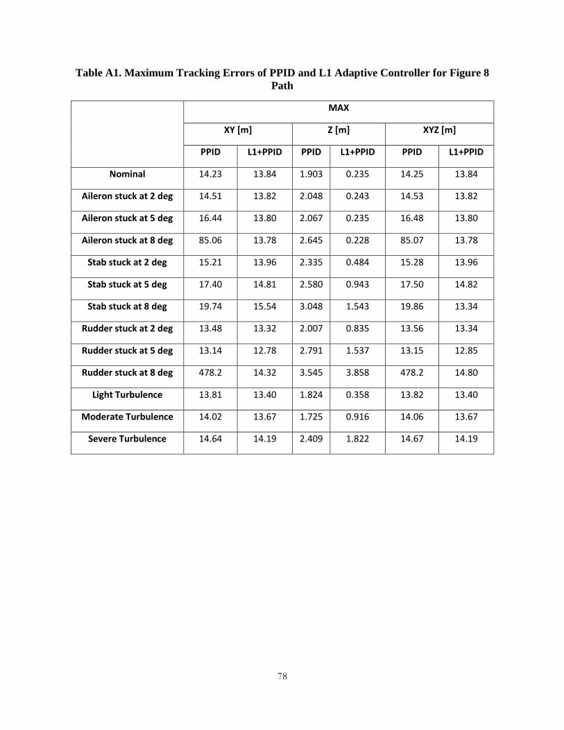
78
Table A1. Maximum Tracking Errors of PPID and L1 Adaptive Controller for Figure 8
Path
MAX
XY [m] Z [m] XYZ [m]
PPID L1+PPID PPID L1+PPID PPID L1+PPID
Nominal 14.23 13.84 1.903 0.235 14.25 13.84
Aileron stuck at 2 deg 14.51 13.82 2.048 0.243 14.53 13.82
Aileron stuck at 5 deg 16.44 13.80 2.067 0.235 16.48 13.80
Aileron stuck at 8 deg 85.06 13.78 2.645 0.228 85.07 13.78
Stab stuck at 2 deg 15.21 13.96 2.335 0.484 15.28 13.96
Stab stuck at 5 deg 17.40 14.81 2.580 0.943 17.50 14.82
Stab stuck at 8 deg 19.74 15.54 3.048 1.543 19.86 13.34
Rudder stuck at 2 deg 13.48 13.32 2.007 0.835 13.56 13.34
Rudder stuck at 5 deg 13.14 12.78 2.791 1.537 13.15 12.85
Rudder stuck at 8 deg 478.2 14.32 3.545 3.858 478.2 14.80
Light Turbulence 13.81 13.40 1.824 0.358 13.82 13.40
Moderate Turbulence 14.02 13.67 1.725 0.916 14.06 13.67
Severe Turbulence 14.64 14.19 2.409 1.822 14.67 14.19

79
Table A2. Mean Tracking Errors of PPID and L1 Adaptive Controller for Figure 8 Path
Mean
XY [m] Z [m] XYZ [m]
PPID L1+PPID PPID L1+PPID PPID L1+PPID
Nominal 5.663 5.486 0.655 0.073 5.723 5.487
Aileron stuck at 2 deg 5.878 5.498 0.675 0.070 5.941 5.499
Aileron stuck at 5 deg 6.171 5.488 0.693 0.068 6.235 5.489
Aileron stuck at 8 deg 26.04 5.476 0.969 0.068 26.10 5.477
Stab stuck at 2 deg 6.061 5.710 0.841 0.165 6.153 5.713
Stab stuck at 5 deg 6.502 5.946 0.930 0.302 6.604 5.957
Stab stuck at 8 deg 7.037 6.111 1.021 0.450 7.152 6.137
Rudder stuck at 2 deg 5.197 5.169 0.556 0.270 5.259 5.179
Rudder stuck at 5 deg 4.736 4.796 0.626 0.523 4.828 4.839
Rudder stuck at 8 deg 123.0 8.832 0.824 1.018 123.1 8.926
Light Turbulence 5.627 5.472 0.696 0.138 5.711 5.479
Moderate Turbulence 5.729 5.539 0.808 0.328 5.851 5.582
Severe Turbulence 6.126 5.904 1.035 0.632 6.318 6.005

80
Table A3. Standard Deviation of Tracking Errors of PPID and L1 Adaptive Controller for
Figure 8 Path
Standard Deviation
XY [m] Z [m] XYZ [m]
PPID L1+PPID PPID L1+PPID PPID L1+PPID
Nominal 4.189 4.194 0.451 0.045 4.183 4.194
Aileron stuck at 2 deg 4.414 4.104 0.473 0.043 4.406 4.104
Aileron stuck at 5 deg 4.719 4.096 0.487 0.043 4.711 4.096
Aileron stuck at 8 deg 27.32 4.090 0.711 0.046 27.29 4.089
Stab stuck at 2 deg 4.459 4.247 0.558 0.119 4.448 4.247
Stab stuck at 5 deg 4.734 4.357 0.629 0.225 4.725 4.357
Stab stuck at 8 deg 5.064 4.400 0.709 0.341 5.056 4.400
Rudder stuck at 2 deg 3.977 4.005 0.529 0.211 3.970 4.007
Rudder stuck at 5 deg 3.803 3.848 0.725 0.418 3.808 3.851
Rudder stuck at 8 deg 157.2 2.968 0.941 0.975 157.2 3.020
Light Turbulence 4.220 4.153 0.449 0.088 4.189 4.147
Moderate Turbulence 4.182 4.171 0.495 0.223 4.120 4.132
Severe Turbulence 4.097 4.075 0.637 0.439 3.985 3.998

81
Table A4. Integral of Control Surface Deflection Rate of PPID and L1 Adaptive Controller
for Figure 8 Path
Integral Of Control Surface Rate Of Change
Elevator [rad/s] x e-03
Aileron [rad/s] x e-03
Rudder[rad/s] x e-03 Throttle [%]
PPID L1+PPID PPID L1+PPID PPID L1+PPID PPID L1+PPID
Nominal 2.194 2.058 12.86 18.01 4.004 0.346 0.522 0.364
Aileron stuck at 2 deg 2.375 2.797 24.34 49.90 4.049 0.956 0.564 0.372
Aileron stuck at 5 deg 2.514 2.784 24.80 50.34 4.241 0.965 0.606 0.372
Aileron stuck at 8 deg 3.442 3.053 25.21 53.57 4.102 1.026 2.401 0.372
Stab stuck at 2 deg 4.722 13.10 13.59 31.68 3.949 0.610 0.602 0.392
Stab stuck at 5 deg 6.191 23.12 15.01 51.18 4.150 0.984 0.658 0.436
Stab stuck at 8 deg 7.604 56.84 16.80 119.1 4.713 2.291 0.712 0.626
Rudder stuck at 2 deg 2.131 2.579 12.39 18.37 4.222 0.354 0.457 0.365
Rudder stuck at 5 deg 2.259 3.615 13.12 24.42 5.031 0.470 0.465 0.403
Rudder stuck at 8 deg 2.387 22.74 9.518 89.88 6.252 1.729 0.391 0.872
Light Turbulence 9.480 19.28 43.50 100.7 12.03 1.862 0.571 0.430
Moderate Turbulence 26.70 56.29 79.91 183.1 26.27 3.375 0.756 0.649
Severe Turbulence 51.74 112.0 139.8 291.36 50.17 5.338 1.134 1.052

82
Table A5. Saturation Index of PPID and L1 Adaptive Controller for Figure 8 Path
Saturation Index
Elevator [rad/s] x e-03
Aileron [rad/s] x e-03
Rudder[rad/s] x e-03 Throttle [%]
PPID L1+PPID PPID L1+PPID PPID L1+PPID PPID L1+PPID
Nominal 0 0 0 0 0 0 0 0
Aileron stuck at 2 deg 0 0 2953 2352 0 0 0 0
Aileron stuck at 5 deg 0 0 6614 4811 0 0 0 0
Aileron stuck at 8 deg 0 0 86053 79384 0 0 14 0
Stab stuck at 2 deg 0 0 0 0 0 0 0 0
Stab stuck at 5 deg 0 0 287 451 0 0 0 0
Stab stuck at 8 deg 0 0 3345 1085 0 0 0 0
Rudder stuck at 2 deg 0 0 0 0 0 0 0 0
Rudder stuck at 5 deg 0 0 0 0 0 0 0 0
Rudder stuck at 8 deg 0 0 1654 7596 0 0 45 0
Light Turbulence 0 0 0 0 0 0 0 0
Moderate Turbulence 0 0 0 0 0 0 0 0
Severe Turbulence 0 0 0 0 0 0 0 0

83
Table A6. Performance Indices of PPID and L1 Adaptive Controller for Figure 8 Path
PI_TT PI_CA PI_TOTAL
PPID L1+PPID PPID L1+PPID PPID L1+PPID
Nominal 0.850 0.863 0.991 0.992 0.892 0.901
Aileron stuck at 2 deg 0.844 0.864 0.985 0.983 0.886 0.899
Aileron stuck at 5 deg 0.833 0.864 0.981 0.981 0.877 0.899
Aileron stuck at 8 deg 0.384 0.864 0.855 0.895 0.525 0.873
Stab stuck at 2 deg 0.838 0.858 0.990 0.987 0.883 0.897
Stab stuck at 5 deg 0.823 0.850 0.988 0.980 0.873 0.889
Stab stuck at 8 deg 0.807 0.843 0.984 0.947 0.860 0.874
Rudder stuck at 2 deg 0.859 0.866 0.992 0.992 0.899 0.903
Rudder stuck at 5 deg 0.863 0.868 0.991 0.990 0.901 0.904
Rudder stuck at 8 deg 0.382 0.823 0.579 0.961 0.441 0.865
Light Turbulence 0.851 0.863 0.981 0.971 0.890 0.896
Moderate Turbulence 0.849 0.859 0.966 0.945 0.884 0.885
Severe Turbulence 0.841 0.850 0.940 0.908 0.871 0.867

84
APPENDIX B
Control Laws Performance over Oval Path

85
Table B1. Maximum Tracking Errors of PPID and L1 Adaptive Controller for Oval Path
MAX
XY [m] Z [m] XYZ [m]
PPID L1+PPID PPID L1+PPID PPID L1+PPID
Nominal 16.29 16.14 1.811 0.166 16.31 16.14
Aileron stuck at 2 deg 16.45 16.12 1.892 0.182 16.48 16.12
Aileron stuck at 5 deg 16.48 16.11 1.908 0.225 16.51 16.11
Aileron stuck at 8 deg 49.17 16.10 1.963 0.268 49.17 16.10
Stab stuck at 2 deg 15.88 16.10 2.555 0.765 15.94 16.10
Stab stuck at 5 deg 16.17 16.45 3.381 1.250 16.24 16.45
Stab stuck at 8 deg 16.56 16.89 4.146 1.770 16.66 15.80
Rudder stuck at 2 deg 15.70 15.80 2.847 1.143 15.76 15.80
Rudder stuck at 5 deg 16.73 15.51 3.843 2.033 16.89 15.57
Rudder stuck at 8 deg 21.35 17.52 5.349 3.324 21.76 17.68
Light Turbulence 16.09 15.72 2.086 0.389 16.12 15.72
Moderate Turbulence 15.96 15.44 2.633 0.903 16.03 15.45
Severe Turbulence 15.91 15.44 3.436 1.643 16.08 15.47

86
Table B2. Mean Tracking Errors of PPID and L1 Adaptive Controller for Oval Path
Mean
XY [m] Z [m] XYZ [m]
PPID L1+PPID PPID L1+PPID PPID L1+PPID
Nominal 7.801 7.606 0.644 0.073 7.842 7.606
Aileron stuck at 2 deg 7.649 7.605 0.659 0.080 7.693 7.606
Aileron stuck at 5 deg 7.282 7.617 0.654 0.092 7.328 7.618
Aileron stuck at 8 deg 16.09 7.630 0.666 0.105 16.13 7.631
Stab stuck at 2 deg 7.287 7.381 0.952 0.253 7.387 7.388
Stab stuck at 5 deg 7.056 7.329 1.142 0.404 7.225 7.347
Stab stuck at 8 deg 6.925 7.348 1.330 0.555 7.200 7.382
Rudder stuck at 2 deg 8.091 7.864 0.999 0.396 8.180 7.879
Rudder stuck at 5 deg 8.435 8.100 1.373 0.720 8.596 8.150
Rudder stuck at 8 deg 9.813 8.676 1.917 1.142 10.07 8.783
Light Turbulence 7.740 7.482 0.689 0.129 7.785 7.484
Moderate Turbulence 7.767 7.466 0.803 0.297 7.829 7.480
Severe Turbulence 7.877 7.591 1.005 0.560 7.980 7.643

87
Table B3. Standard Deviation of Tracking Errors of PPID andL1 Adaptive Controller for
Oval Path
Standard Deviation
XY [m] Z [m] XYZ [m]
PPID L1+PPID PPID L1+PPID PPID L1+PPID
Nominal 4.782 4.744 0.485 0.046 4.783 4.744
Aileron stuck at 2 deg 4.826 4.737 0.501 0.051 4.828 4.736
Aileron stuck at 5 deg 4.860 4.736 0.501 0.059 4.860 4.736
Aileron stuck at 8 deg 15.68 4.737 0.502 0.068 15.67 4.736
Stab stuck at 2 deg 4.603 4.688 0.716 0.179 4.598 4.687
Stab stuck at 5 deg 4.721 4.786 0.885 0.303 4.687 4.785
Stab stuck at 8 deg 4.982 4.958 1.056 0.439 4.879 4.958
Rudder stuck at 2 deg 4.758 4.716 0.750 0.286 4.770 4.716
Rudder stuck at 5 deg 4.949 4.730 1.029 0.526 4.971 4.729
Rudder stuck at 8 deg 5.753 4.573 1.460 0.849 5.822 4.590
Light Turbulence 4.723 4.625 0.536 0.103 4.729 4.624
Moderate Turbulence 4.715 4.619 0.654 0.228 4.726 4.612
Severe Turbulence 4.784 4.671 0.853 0.429 4.797 4.639

88
Table B4. Integral of Control Surface Deflection Rate of PPID and L1 Adaptive Controller
for Oval Path
Integral Of Control Surface Rate Of Change
Elevator [rad/s] x e-03
Aileron [rad/s] x e-03
Rudder[rad/s] x e-03 Throttle [%]
PPID L1+PPID PPID L1+PPID PPID L1+PPID PPID L1+PPID
Nominal 3.076 2.871 15.65 20.24 4.951 0.390 0.820 0.621
Aileron stuck at 2 deg 3.265 3.455 27.51 56.83 4.928 1.089 0.820 0.638
Aileron stuck at 5 deg 3.254 3.336 24.79 56.90 5.007 1.089 0.789 0.641
Aileron stuck at 8 deg 4.252 3.359 23.69 59.31 3.902 1.134 1.802 0.645
Stab stuck at 2 deg 6.449 10.68 16.02 29.52 4.658 0.569 0.906 0.671
Stab stuck at 5 deg 8.386 12.73 17.22 29.91 5.107 0.575 0.989 0.736
Stab stuck at 8 deg 10.37 14.68 19.06 30.78 5.653 0.591 1.085 0.822
Rudder stuck at 2 deg 3.358 3.492 16.61 28.15 6.279 0.544 0.980 0.773
Rudder stuck at 5 deg 3.940 5.723 19.82 48.59 8.395 0.937 1.151 0.934
Rudder stuck at 8 deg 4.358 40.35 24.42 188.0 11.76 3.630 1.346 1.351
Light Turbulence 10.06 19.50 41.39 88.68 11.59 1.644 0.849 0.659
Moderate Turbulence 28.16 57.18 83.25 213.3 27.12 3.926 0.988 0.824
Severe Turbulence 53.77 110.4 151.8 305.6 50.94 5.614 1.280 1.157

89
Table B5. Saturation Index of PPID and L1 Adaptive Controller for Oval Path
Saturation Index
Elevator [rad/s] x e-03
Aileron [rad/s] x e-03
Rudder[rad/s] x e-03 Throttle [%]
PPID L1+PPID PPID L1+PPID PPID L1+PPID PPID L1+PPID
Nominal 0 0 0 0 0 0 0 0
Aileron stuck at 2 deg 0 0 2595 2243 0 0 0 0
Aileron stuck at 5 deg 0 0 6717 4962 0 0 0 0
Aileron stuck at 8 deg 0 0 83908 76903 0 0 0 0
Stab stuck at 2 deg 0 0 0 0 0 0 0 0
Stab stuck at 5 deg 0 0 0 0 0 0 0 0
Stab stuck at 8 deg 0 0 2950 2324 0 0 0 0
Rudder stuck at 2 deg 0 0 0 0 0 0 0 0
Rudder stuck at 5 deg 0 0 0 811 0 0 0 0
Rudder stuck at 8 deg 0 0 1292 3492 0 0 0 0
Light Turbulence 0 0 0 0 0 0 0 0
Moderate Turbulence 0 0 0 0 0 0 0 0
Severe Turbulence 0 0 0 0 0 0 0 0

90
Table B6. Performance Indices of PPID and L1 Adaptive Controller for Oval Path
PI_TT PI_CA PI_TOTAL
PPID L1+PPID PPID L1+PPID PPID L1+PPID
Nominal 0.818 0.830 0.987 0.989 0.863 0.873
Aileron stuck at 2 deg 0.818 0.830 0.982 0.979 0.859 0.870
Aileron stuck at 5 deg 0.821 0.830 0.979 0.976 0.856 0.869
Aileron stuck at 8 deg 0.528 0.830 0.892 0.896 0.331 0.845
Stab stuck at 2 deg 0.820 0.830 0.986 0.985 0.859 0.870
Stab stuck at 5 deg 0.816 0.826 0.984 0.984 0.856 0.866
Stab stuck at 8 deg 0.810 0.819 0.979 0.980 0.846 0.859
Rudder stuck at 2 deg 0.810 0.823 0.985 0.986 0.861 0.869
Rudder stuck at 5 deg 0.795 0.816 0.982 0.979 0.857 0.865
Rudder stuck at 8 deg 0.751 0.800 0.977 0.937 0.846 0.858
Light Turbulence 0.818 0.833 0.979 0.971 0.860 0.864
Moderate Turbulence 0.816 0.831 0.962 0.937 0.856 0.855
Severe Turbulence 0.809 0.824 0.936 0.904 0.850 0.842

91
APPENDIX C
Control Laws Performance over OA Path

92
Table C1. Maximum Tracking Errors of PPID and L1 Adaptive Controller for OA Path
MAX
XY [m] Z [m] XYZ [m]
PPID L1+PPID PPID L1+PPID PPID L1+PPID
Nominal 19.84 19.99 2.213 0.227 19.94 19.99
Aileron stuck at 2 deg 19.83 19.83 2.344 0.277 19.93 19.83
Aileron stuck at 5 deg 19.96 19.84 2.345 0.318 20.06 19.84
Aileron stuck at 8 deg 2745 19.85 2.606 0.359 2745 19.85
Stab stuck at 2 deg 19.94 19.95 2.951 0.893 20.06 19.95
Stab stuck at 5 deg 20.02 19.93 3.319 1.436 20.12 19.93
Stab stuck at 8 deg 20.97 19.78 3.712 2.005 21.04 19.87
Rudder stuck at 2 deg 19.67 19.87 3.329 1.347 19.73 19.87
Rudder stuck at 5 deg 19.18 19.40 4.424 2.520 19.21 19.41
Rudder stuck at 8 deg 18.47 17.85 5.757 4.319 18.88 17.88
Light Turbulence 19.74 19.92 2.102 0.433 19.85 19.92
Moderate Turbulence 19.52 19.56 2.225 1.066 19.65 19.56
Severe Turbulence 19.14 19.02 2.556 2.096 19.29 19.03

93
Table C2. Mean Tracking Errors of PPID and L1 Adaptive Controller for OA Path
Mean
XY [m] Z [m] XYZ [m]
PPID L1+PPID PPID L1+PPID PPID L1+PPID
Nominal 8.075 7.849 0.950 0.090 8.168 7.851
Aileron stuck at 2 deg 8.175 7.774 0.977 0.088 8.267 7.775
Aileron stuck at 5 deg 8.253 7.766 0.984 0.092 8.345 7.768
Aileron stuck at 8 deg 972.9 7.757 0.666 0.101 972.9 7.759
Stab stuck at 2 deg 8.122 7.791 1.123 0.333 8.251 7.807
Stab stuck at 5 deg 8.274 7.850 1.211 0.604 8.425 7.896
Stab stuck at 8 deg 8.610 7.923 1.334 0.875 8.795 8.015
Rudder stuck at 2 deg 7.923 7.723 1.095 0.590 8.076 7.768
Rudder stuck at 5 deg 7.894 7.580 1.629 1.141 8.190 7.734
Rudder stuck at 8 deg 9.072 8.324 2.471 1.836 9.558 8.618
Light Turbulence 8.090 7.813 0.902 0.117 8.172 7.815
Moderate Turbulence 8.168 7.876 0.827 0.290 8.239 7.888
Severe Turbulence 8.442 8.133 0.817 0.578 8.513 8.178

94
Table C3. Standard Deviation of Tracking Errors of PPID and L1 Adaptive Controller for
OA Path
Standard Deviation
XY [m] Z [m] XYZ [m]
PPID L1+PPID PPID L1+PPID PPID L1+PPID
Nominal 4.182 4.252 0.586 0.058 4.151 4.251
Aileron stuck at 2 deg 4.179 4.203 0.604 0.058 4.156 4.202
Aileron stuck at 5 deg 4.286 4.196 0.607 0.065 4.264 4.195
Aileron stuck at 8 deg 892.1 4.189 0.748 0.079 892.1 4.187
Stab stuck at 2 deg 4.218 4.209 0.725 0.201 4.179 4.198
Stab stuck at 5 deg 4.331 4.205 0.834 0.354 4.287 4.177
Stab stuck at 8 deg 4.604 4.179 0.971 0.515 4.549 4.126
Rudder stuck at 2 deg 4.131 4.181 0.898 0.346 4.076 4.154
Rudder stuck at 5 deg 4.007 3.994 1.114 0.670 3.899 3.918
Rudder stuck at 8 deg 3.458 3.171 1.471 1.087 3.342 3.103
Light Turbulence 4.138 4.202 0.558 0.092 4.113 4.200
Moderate Turbulence 4.085 4.116 0.556 0.236 4.065 4.110
Severe Turbulence 4.004 3.941 0.628 0.476 3.985 3.920
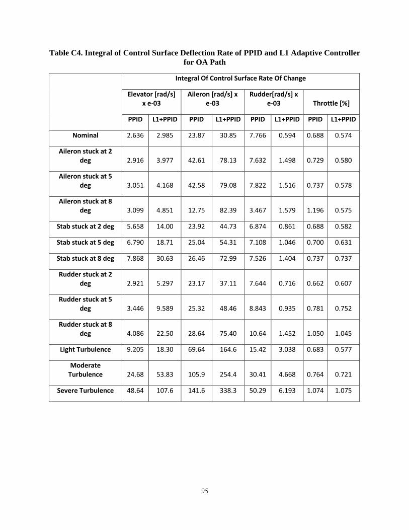
95
Table C4. Integral of Control Surface Deflection Rate of PPID and L1 Adaptive Controller
for OA Path
Integral Of Control Surface Rate Of Change
Elevator [rad/s] x e-03
Aileron [rad/s] x e-03
Rudder[rad/s] x e-03 Throttle [%]
PPID L1+PPID PPID L1+PPID PPID L1+PPID PPID L1+PPID
Nominal 2.636 2.985 23.87 30.85 7.766 0.594 0.688 0.574
Aileron stuck at 2 deg 2.916 3.977 42.61 78.13 7.632 1.498 0.729 0.580
Aileron stuck at 5 deg 3.051 4.168 42.58 79.08 7.822 1.516 0.737 0.578
Aileron stuck at 8 deg 3.099 4.851 12.75 82.39 3.467 1.579 1.196 0.575
Stab stuck at 2 deg 5.658 14.00 23.92 44.73 6.874 0.861 0.688 0.582
Stab stuck at 5 deg 6.790 18.71 25.04 54.31 7.108 1.046 0.700 0.631
Stab stuck at 8 deg 7.868 30.63 26.46 72.99 7.526 1.404 0.737 0.737
Rudder stuck at 2 deg 2.921 5.297 23.17 37.11 7.644 0.716 0.662 0.607
Rudder stuck at 5 deg 3.446 9.589 25.32 48.46 8.843 0.935 0.781 0.752
Rudder stuck at 8 deg 4.086 22.50 28.64 75.40 10.64 1.452 1.050 1.045
Light Turbulence 9.205 18.30 69.64 164.6 15.42 3.038 0.683 0.577
Moderate Turbulence 24.68 53.83 105.9 254.4 30.41 4.668 0.764 0.721
Severe Turbulence 48.64 107.6 141.6 338.3 50.29 6.193 1.074 1.075

96
Table C5. Saturation Index of PPID and L1 Adaptive Controller for OA Path
Saturation Index
Elevator [rad/s] x e-03
Aileron [rad/s] x e-03
Rudder[rad/s] x e-03 Throttle [%]
PPID L1+PPID PPID L1+PPID PPID L1+PPID PPID L1+PPID
Nominal 0 0 0 0 0 0 0 0
Aileron stuck at 2 deg 0 0 3692 3053 0 0 0 0
Aileron stuck at 5 deg 0 0 8925 6895 0 0 0 0
Aileron stuck at 8 deg 0 0 93050 80547 0 0 80 0
Stab stuck at 2 deg 0 0 0 0 0 0 0 0
Stab stuck at 5 deg 0 0 0 444 0 0 0 0
Stab stuck at 8 deg 0 0 4241 6171 0 0 0 0
Rudder stuck at 2 deg 0 0 0 0 0 0 0 0
Rudder stuck at 5 deg 0 0 0 0 0 0 0 0
Rudder stuck at 8 deg 0 0 0 2187 0 0 0 0
Light Turbulence 0 0 0 0 0 0 0 0
Moderate Turbulence 0 0 0 0 0 0 0 0
Severe Turbulence 0 0 0 38 0 0 0 0
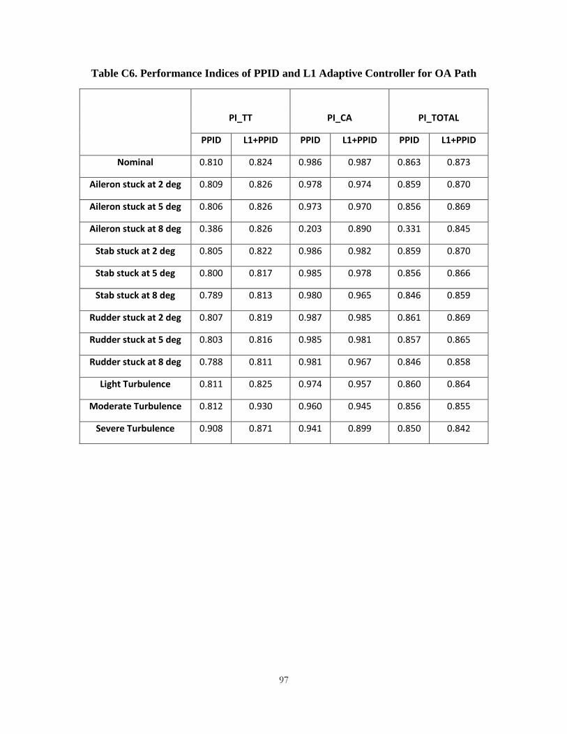
97
Table C6. Performance Indices of PPID and L1 Adaptive Controller for OA Path
PI_TT PI_CA PI_TOTAL
PPID L1+PPID PPID L1+PPID PPID L1+PPID
Nominal 0.810 0.824 0.986 0.987 0.863 0.873
Aileron stuck at 2 deg 0.809 0.826 0.978 0.974 0.859 0.870
Aileron stuck at 5 deg 0.806 0.826 0.973 0.970 0.856 0.869
Aileron stuck at 8 deg 0.386 0.826 0.203 0.890 0.331 0.845
Stab stuck at 2 deg 0.805 0.822 0.986 0.982 0.859 0.870
Stab stuck at 5 deg 0.800 0.817 0.985 0.978 0.856 0.866
Stab stuck at 8 deg 0.789 0.813 0.980 0.965 0.846 0.859
Rudder stuck at 2 deg 0.807 0.819 0.987 0.985 0.861 0.869
Rudder stuck at 5 deg 0.803 0.816 0.985 0.981 0.857 0.865
Rudder stuck at 8 deg 0.788 0.811 0.981 0.967 0.846 0.858
Light Turbulence 0.811 0.825 0.974 0.957 0.860 0.864
Moderate Turbulence 0.812 0.930 0.960 0.945 0.856 0.855
Severe Turbulence 0.908 0.871 0.941 0.899 0.850 0.842

98
APPENDIX D
Control Laws Performance over 3D S Turns Path

99
Table D1. Maximum Tracking Errors of PPID and L1 Adaptive Controller for 3D S-Turns
MAX
XY [m] Z [m] XYZ [m]
PPID L1+PPID PPID L1+PPID PPID L1+PPID
Nominal 26.58 35.43 5.453 3.387 26.60 35.43
Aileron stuck at 2 deg 28.93 35.44 6.379 3.419 29.02 35.45
Aileron stuck at 5 deg 35.70 35.44 6.233 3.471 35.76 35.44
Aileron stuck at 8 deg 849.1 35.43 6.733 3.523 849.2 35.44
Stab stuck at 2 deg 36.03 35.66 4.437 3.991 36.09 35.69
Stab stuck at 5 deg 36.46 35.99 5.252 4.477 36.54 36.03
Stab stuck at 8 deg 44.81 35.85 6.011 4.868 44.81 35.09
Rudder stuck at 2 deg 25.85 35.04 5.188 4.574 25.89 35.09
Rudder stuck at 5 deg 23.91 33.77 7.075 5.857 24.07 33.90
Rudder stuck at 8 deg 28.64 31.11 7.662 7.878 28.85 31.45
Light Turbulence 25.89 35.01 5.399 3.394 25.90 35.01
Moderate Turbulence 25.29 34.27 5.368 3.422 25.32 34.28
Severe Turbulence 25.47 33.57 6.082 3.549 25.49 33.59

100
Table D2. Mean Tracking Errors of PPID and L1 Adaptive Controller for 3D S Turns
Mean
XY [m] Z [m] XYZ [m]
PPID L1+PPID PPID L1+PPID PPID L1+PPID
Nominal 10.49 14.53 1.310 0.748 10.65 14.59
Aileron stuck at 2 deg 11.17 14.51 1.292 0.757 11.34 14.57
Aileron stuck at 5 deg 12.96 14.51 1.336 0.770 13.13 14.57
Aileron stuck at 8 deg 159.7 14.51 1.992 0.784 159.7 14.57
Stab stuck at 2 deg 14.52 14.35 1.188 0.948 14.64 14.43
Stab stuck at 5 deg 14.50 14.23 1.340 1.150 14.66 14.34
Stab stuck at 8 deg 15.83 13.94 1.442 1.343 16.04 14.09
Rudder stuck at 2 deg 10.56 14.60 1.433 1.175 10.75 14.71
Rudder stuck at 5 deg 10.71 14.54 1.789 1.674 10.98 14.72
Rudder stuck at 8 deg 12.33 14.66 2.298 2.415 12.70 14.98
Light Turbulence 10.31 14.41 1.351 0.789 10.49 14.47
Moderate Turbulence 10.04 14.21 1.420 0.918 10.24 14.29
Severe Turbulence 9.633 13.91 1.658 1.170 9.932 14.03
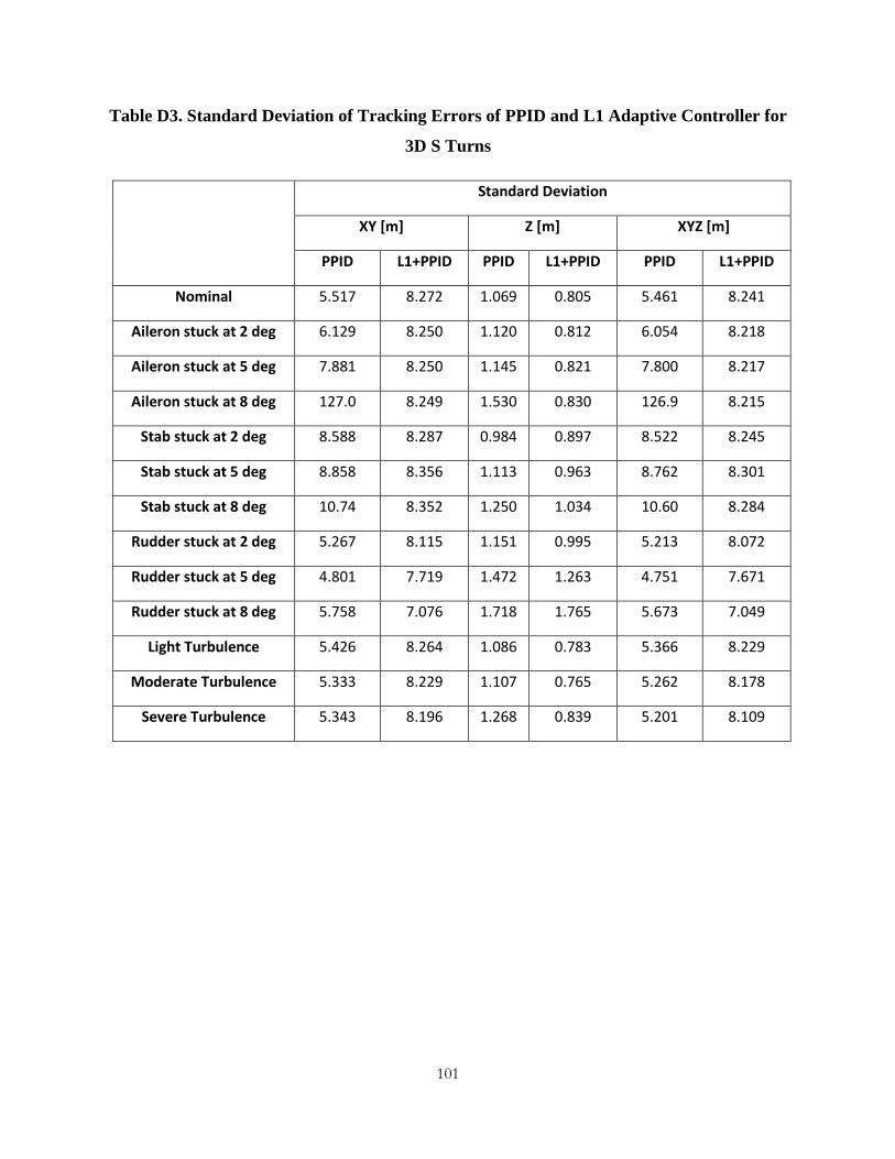
101
Table D3. Standard Deviation of Tracking Errors of PPID and L1 Adaptive Controller for
3D S Turns
Standard Deviation
XY [m] Z [m] XYZ [m]
PPID L1+PPID PPID L1+PPID PPID L1+PPID
Nominal 5.517 8.272 1.069 0.805 5.461 8.241
Aileron stuck at 2 deg 6.129 8.250 1.120 0.812 6.054 8.218
Aileron stuck at 5 deg 7.881 8.250 1.145 0.821 7.800 8.217
Aileron stuck at 8 deg 127.0 8.249 1.530 0.830 126.9 8.215
Stab stuck at 2 deg 8.588 8.287 0.984 0.897 8.522 8.245
Stab stuck at 5 deg 8.858 8.356 1.113 0.963 8.762 8.301
Stab stuck at 8 deg 10.74 8.352 1.250 1.034 10.60 8.284
Rudder stuck at 2 deg 5.267 8.115 1.151 0.995 5.213 8.072
Rudder stuck at 5 deg 4.801 7.719 1.472 1.263 4.751 7.671
Rudder stuck at 8 deg 5.758 7.076 1.718 1.765 5.673 7.049
Light Turbulence 5.426 8.264 1.086 0.783 5.366 8.229
Moderate Turbulence 5.333 8.229 1.107 0.765 5.262 8.178
Severe Turbulence 5.343 8.196 1.268 0.839 5.201 8.109

102
Table D4. Integral of Control Surface Deflection Rate of PPID and L1 Adaptive Controller
for 3D S Turns
Integral Of Control Surface Rate Of Change
Elevator [rad/s] x e-03
Aileron [rad/s] x e-03
Rudder[rad/s] x e-03 Throttle [%]
PPID L1+PPID PPID L1+PPID PPID L1+PPID PPID L1+PPID
Nominal 2895 12.22 938.8 28.30 369.4 0.545 15.31 1.245
Aileron stuck at 2 deg 2758 12.89 977.5 70.08 286.3 1.342 17.07 1.246
Aileron stuck at 5 deg 2760 12.81 842.4 69.58 220.0 1.333 17.11 1.247
Aileron stuck at 8 deg 3180 12.85 430.3 70.37 123.9 1.347 1.911 1.248
Stab stuck at 2 deg 39.97 27.78 37.62 68.10 8.976 1.308 1.381 1.289
Stab stuck at 5 deg 38.05 44.10 36.59 102.3 8.915 1.965 1.407 1.415
Stab stuck at 8 deg 34.52 81.46 34.03 177.1 8.267 3.403 1.494 1.747
Rudder stuck at 2 deg 2886 12.82 831.3 32.64 453.9 0.629 15.36 1.290
Rudder stuck at 5 deg 2848 15.22 843.9 46.28 414.2 0.891 15.94 1.380
Rudder stuck at 8 deg 2826 29.29 799.8 103.1 414.5 1.989 14.58 1.598
Light Turbulence 2895 29.04 941.6 91.29 369.0 1.698 15.34 1.231
Moderate Turbulence 2895 68.31 954.0 182.2 371.4 3.367 15.38 1.320
Severe Turbulence 2873 125.2 887.5 292.4 363.2 5.371 15.74 1.584

103
Table D5. Saturation Index of PPID and L1 Adaptive Controller for 3D S Turns
Saturation Index
Elevator [rad/s] x e-03
Aileron [rad/s] x e-03
Rudder[rad/s] x e-03 Throttle [%]
PPID L1+PPID PPID L1+PPID PPID L1+PPID PPID L1+PPID
Nominal 83360 0 23958 0 0 0 0 0
Aileron stuck at 2 deg 84630 0 44415 3162 0 0 0 0
Aileron stuck at 5 deg 84770 0 48628 7166 0 0 0 0
Aileron stuck at 8 deg 83985 0 79337 77082 0 0 84 0
Stab stuck at 2 deg 252 0 266 245 0 0 0 0
Stab stuck at 5 deg 292 0 1530 1336 0 0 0 0
Stab stuck at 8 deg 358 0 3789 14650 0 0 0 0
Rudder stuck at 2 deg 83469 0 23691 0 0 0 0 0
Rudder stuck at 5 deg 83801 0 25076 338 0 0 0 0
Rudder stuck at 8 deg 84003 0 34612 1358 0 0 9 7
Light Turbulence 83379 0 24046 0 0 0 0 0
Moderate Turbulence 83376 0 24179 0 0 0 0 0
Severe Turbulence 83611 0 20953 0 0 0 2 0

104
Table D6. Performance Indices of PPID and L1 Adaptive Controller for 3D S Turns
PI_TT PI_CA PI_TOTAL
PPID L1+PPID PPID L1+PPID PPID L1+PPID
Nominal 0.743 0.659 0.466 0.979 0.660 0.755
Aileron stuck at 2 deg 0.722 0.660 0.443 0.968 0.638 0.752
Aileron stuck at 5 deg 0.667 0.660 0.452 0.964 0.603 0.751
Aileron stuck at 8 deg 0.364 0.659 0.135 0.885 0.295 0.727
Stab stuck at 2 deg 0.648 0.657 0.968 0.967 0.744 0.750
Stab stuck at 5 deg 0.641 0.654 0.967 0.955 0.739 0.744
Stab stuck at 8 deg 0.583 0.655 0.966 0.915 0.698 0.733
Rudder stuck at 2 deg 0.746 0.655 0.449 0.978 0.657 0.752
Rudder stuck at 5 deg 0.746 0.656 0.448 0.973 0.657 0.751
Rudder stuck at 8 deg 0.702 0.656 0.436 0.941 0.622 0.741
Light Turbulence 0.747 0.662 0.465 0.963 0.663 0.752
Moderate Turbulence 0.752 0.665 0.464 0.936 0.665 0.746
Severe Turbulence 0.751 0.668 0.462 0.900 0.665 0.737