Embed Size (px)
Citation preview

Fault-Tolerance in Multi-Computer Networks
by
CHAU, Siu-Cheung
B.Ed., University of Lethbridge, 1983 M.Sc., Simon Fraser University, 1984
A THESIS SUBMITTED IN PARTIAL FULFILLMENT OF THE REQUIREMENTS FOR THE DEGREE OF
Doctor of Philosophy in the School
of Computing Science
O CHAU, Siu-Cheung 1989
SIMON FRASER UNIVERSITY
August 1989
All rights reserved. This thesis may not be reproduced in whole or in part, by photocopy
or other means, without the permission of the author.

Approval
Name: Siu-Cheung Chau
Degree: Doctor of Philosophy
Title of Thesis: Fault-Tolerance in Multi-Computer Networks
Dr. Pavol Hell, h a i m G
Dr. Artnur L. Liestman, Senior Supervisor
Er. J s ph Peters, Supervisor v
Dr. Ramesh ~rishnamurti, Supervisor
Dr. Frank Ruskey, ExtemAl Examiner
Date Approved

PARTIAL COPYRIGHT LICENSE
I hereby grant t o Simon Fraser Univers i ty the r i g h t t o lend
my thesis, proJect o r extended essay ( the t i t l e o f which i s shown below)
t o users o f the Simon Fraser Univers i ty Library, and t o make p a r t i a l o r
s ing le copies only f o r such users o r i n response t o a request from the
l i b r a r y o f any other un ivers i ty , o r o ther educational i n s t i t u t i o n , on
i t s own behalf o r f o r one of I t s users. I fu r ther agree t h a t permission
f o r mu l t i p l e copying of t h i s work f o r scholar ly purposes may be granted
by me o r the Dean o f Graduate Studies. i t i s understood t h a t copying
o r pub l i ca t ion o f t h i s work f o r f i nanc ia l gain sha l l not be allowed
without my wr i t t en permission.
T i t l e o f Thes i s/Project/Extended Essay
Fault-Tolerance i n Mult i-Computer Networks.
Author: - --
(signature)
S iu-Cheung Chau
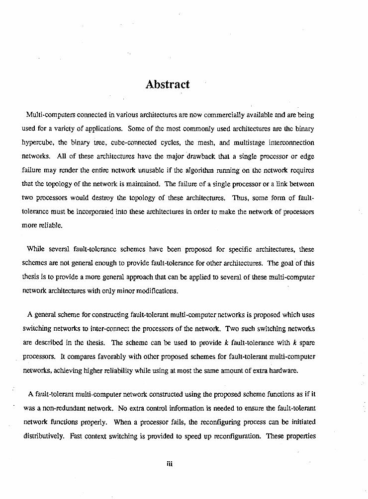
Abstract
Multi-computers connected in various architectures are now commercially available and are being
used for a variety of applications. Some of the most commonly used architectures are the binary
hypercube, the binary tree, cube-connected cycles, the mesh, and multistage interconnection
networks. All of these architectures have the major drawback that a single processor or edge
failure may render the entire network unusable if the algorithm running on the network requires
that the topology of the network is maintained. The failure of a single processor or a link between
two processors would destroy the topology of these architectures. Thus, some form of fault-
tolerance must be incorporated into these architectures in order to make the network of processors
more reliable.
While several fault-tolerance schemes have been proposed for specific architectures, these
schemes are not general enough to provide fault-tolerance for other architectures. The goal of this
thesis is to provide a more general approach that can be applied to several of these multi-computer
network architectures with only minor modifications.
A general scheme for constructing fault-tolerant multi-computer networks is proposed which uses
switching networks to inter-connect the processors of the network. Two such switching networks
are described in the thesis. The scheme can be used to provide k fault-tolerance with k spare
processors. It compares favorably with other proposed schemes for fault-tolerant multi-computer
networks, achieving higher reliability while using at most the same amount of extra hardware.
A fault-tolerant multi-computer network constructed using the proposed scheme functions as if it
was a non-redundant network. No extra control information is needed to ensure the fault-tolerant
network functions properly. When a processor fails, the reconfiguring process can be initiated
distributively. Fast context switching is provided to speed up reconfiguration. These properties
iii

together with the ability to provide high level of reliability for a long period of time make our
scheme suitable for long-life unmaintained applications.

To my wife L i y and my daughter Lilian
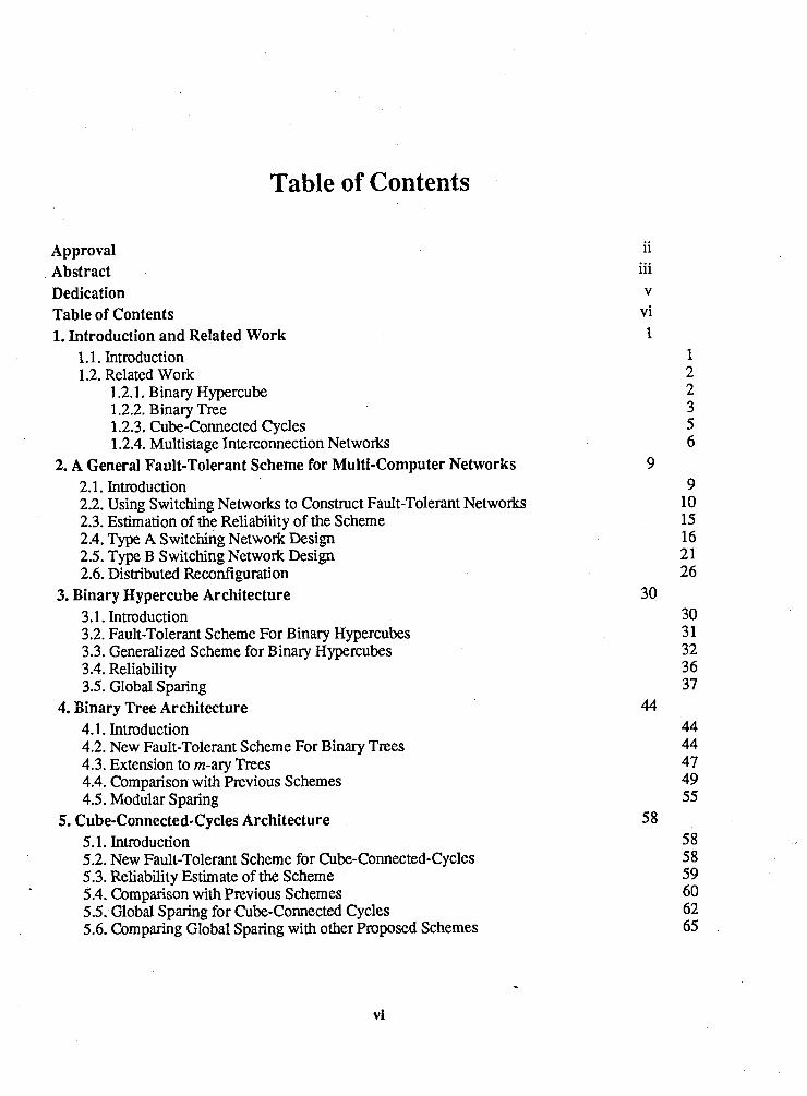
Table of Contents
Approval Abstract Dedication Table of Contents 1. Introduction and Related Work
1.1. Introduction 1.2. Related Work
1.2.1. Binary Hypercube 1.2.2. Binary Tree 1.2.3. Cube-Connected Cycles 1.2.4. Multistage Interconnection Networks
2. A General Fault-Tolerant Scheme for Multi-Computer Networks 2.1. Introduction 2.2. Using Switching Networks to Construct Fault-Tolerant Networks 2.3. Estimation of the Reliability of the Scheme 2.4. Type A Switching Network Design 2.5. Type B Switching Network Design 2.6. Distributed Reconfiguration
3. Binary Hypercube Architecture 3.1. Introduction 3.2. Fault-Tolerant Scheme For Binary Hypercubes 3.3. Generalized Scheme for Binary Hypercubes 3.4. Reliability 3.5. Global Sparing
4. Binary Tree Architecture 4.1. Introduction 4.2. New Fault-Tolerant Scheme For Binary Trees 4.3. Extension to m-ary Trees 4.4. Comparison with Previous Schemes 4.5. Modular Sparing
5. Cube-Connected-Cycles Architecture 5.1. Introduction 5.2. New Fault-Tolerant Scheme for Cube-Connected-Cycles 5.3. Reliability Estimate of the Scheme 5.4. Comparison with Previous Schemes 5.5. Global Sparing for Cube-Connected Cycles 5.6. Comparing Global Sparing with other Proposed Schemes
ii iii v vi 1
1 2 2 3 5 6
9 9
10 15 16 2 1 26
30 30 3 1 32 36 37
44 44 44 47 49 55
5 8 58 58 59 60 62 65

6. Multistage Interconnection Networks 6.1. Introduction 6.2. New Fault-Tolerant Scheme For Multistage Interconnection Networks 6.3. Reliability Estimation of the Scheme 6.4. Extension to Cover Switching Element Failures 6.5. Reliability of the Extended Scheme 6.6. Modular Sparing
7. Conclusion References
vii

List of Tables
Table 3-1:
Table 3-2:
Table 3-3:
Table 3-4:
Table 4-1:
Table 4-2:
Table 4-3:
Table 4-4:
Table 4-5:
Table 5-1:
Table 5-2:
Table 6-1:
Table 6-2:
Table 6-3: Table 6-4:
Table 6-5:
Table 6-6:
Table 6-7:
Number of spares required for Rennels' basic scheme and our scheme to achieve the same level of reliability at time t= 0.05 and c = 1 Number of spares required for Rennels' hierarchical scheme and our scheme to achieve the same level of reliability at time t= 1 and c= 1 Extra hardware required for global sparing and modular sparing with 2 fault- tolerant modules having a reliability of at least 0.98 at t= 0.1 and c = 1 Extra hardware required for modular sparing with 4, 8, and 16 fault-tolerant modules having a reliability of at least 0.98 at t=0.1 and c= 1 Hardware requirements for Lowrie and Fuch's SOFT scheme and our new scheme to achieve the same level of reliability at t=0.2 Hardware requirements for Singh's scheme and our new scheme to achieve the same level of reliability at t=0.2 Hardware requirements for Howell and Agarwal's scheme and our new scheme to achieve the same level of reliability at t=0.2 Hardware requirements for Howell and Agarwal's scheme and our new scheme to achieve a reliability of at least 0.98 at t=0.4 The amount of extra hardware required to achieve the same level of reliability for the modular and for the global scheme at t=0.4 The number of spares required to achieve the same level of system reliability for Bane rjee's modular sparing scheme and the global sparing scheme using h=O.l, t=0.1, c= 1 and h=d if d is even or h=d+ 1 if d is odd The number of spares required to achieve the same level of system reliability for the new modular sparing scheme and the global sparing scheme at t=0.2 and h=d The system reliability of Jeng and Siegel's DR scheme and our new scheme with k=2 The system reliability of Jeng and Siegel's DR scheme and our new scheme with one spare processor and one spare switching element per stage The system reliability of our new scheme with different values of k and f The number of spare processors, k, and spare switching element, f, per stage required to achieve a reliability of at least 0.98 Extra hardware required for global sparing and modular sparing with 2, and 4 modules having the same level of reliability at t=0.01 and c= 1 Extra hardware required for global sparing and modular sparing using the extended scheme at t=0.01 and c= 1 Extra hardware required for global sparing and modular sparing using the extended scheme at t= 0.1 and c= 1
viii

List of Figures
Figure 1-1: A 3-dimensional binary hypercube Figure 1-2: A cube-connected cycles with h =4 and d = 2 Figure 1-3: A shuffle exchange network with 8 processors Figure 2-1: A switching network with n incoming links and n+k outgoing links Figure 2-2: Using switching networks to connect two fault-tolerant modules Figure 2-3: Using direct connection to construct a fault-tolerant cycle of six processors Figure 2-4: Connecting a cycle with 6 active processors and 1 spare processor using
two switching networks Figure 2-5: Connecting a network with two cycles of six processors and two spare
processors using three switching networks Figure 2-6: 3 decoupling networks arranged in 3 levels Figure 2-7: Connections after processor 3 has failed Figure 2-8: Connections after processor 1 and 3 have failed Figure 2-9: Connections after processor 1,3 and 7 have failed Figure 2-10: Connections after processor 3 has become faulty Figure 2-11: Connections after processor 3 and 7 have become faulty Figure 2-12: Connections after processor 1 ,3 and 7 have become faulty Figure 2-13: For n=8 and k = 4 , some switches do not have to be switchable Figure 2-14: Connections between the processors Figure 3-1: Figure 3-2: Figure 3-3: Figure 3-4: Figure 3-5:
Figure 3-6:
Figure 3-7:
Figure 4-1: Figure 4-2: Figure 4-3:
Figure 4-4:
Figure 4-5: Figure 4-6:
Figure 4-7:
Figure 5-1: Figure 5-2:
A fault-tolerant module with k spares Connections after processor 3 has become faulty Connections after processor 1 has become faulty Connections after processor 5 has become faulty Using 2 Type A switching networks to form a fault-tolerant 2-dimensional binary hypercube Using 3 Type A switching networks to form a fault-tolerant 3-dimensional binary hypercube System reliability of Rennels' scheme with 369 spares and our scheme with 43 spares for n= 8 A fault-tolerant 3-level binary tree with 1 spare A 2-fault-tolerant 3-level binary tree Connections in the fault-tolerant 3-level binary tree with 2 spares after processor 3 has become faulty Connections in the fault-tolerant 3-level binary tree with 2 spares after processors 3 and 7 have failed A fault-tolerant 2-level 3-ary tree with 1 spare System reliabilities of the four schemes for an 8-level binary tree using c= 1 System reliabilities of the four schemes for an 8-level binary tree using c=0.95 A fault-tolerant cycle with k spares Comparing system reliability of Bane jee's basic scheme and our scheme with d=3 and h=8, and d=5 and h=32

Figure 5-3:
Figure 5-4:
Figure 5-5:
Figure 5-6: Figure 6-1: Figure 6-2: Figure 6-3: Figure 6-4:
Comparing system reliability of Banerjee's modular scheme using g=h/2 62 and our scheme with d=5 and h= 6, and d= 6 and h= 8 Using 2 Type A switching networks to connect 4 processors together to 63 form a cycle Connecting 10 processors into 2 cycles with 5 processors each using 3 64 switching networks A fault-tolerant CCC with d=2, h = 4 and 1 spare for the entire network 65 A multistage interconnection network 69 A fault-tolerant multistage interconnection network 70 A shuffle exchange network with 8 processors 74 The connection between 4 groups of switching networks 74

Chapter 1
Introduction and Related Work
1.1. Introduction
Multi-computers connected in various architectures are now commercially available and are being
used for a variety of applications. Some of the most commonly used architectures are the binary
hypercube, binary tree, cube-connected cycles, mesh, and multistage interconnection networks. All
of these architectures have the major drawback that a single processor or edge failure may render
the entire network unusable if the algorithm xunning on the network requires that the topology of
the network does not change. The failure of a single processor or the failure of a l i i between two
processors would destroy the topology of these architectures. Thus, some form of fault-tolerance
must be incorporated into these architectures in order to make the network of processors more
reliable.
Several fault-tolerance schemes have been proposed which can only be applied to a particular
architecture. These proposed schemes are not general enough to provide fault-tolerance for any
architecture. The goal of this thesis is to propose a more general fault-tolerant approach that can be
applied to several of these multi-computer network architectures with only minor modifications.
This scheme described in Chapter 2, provides higher reliability than the previously proposed
schemes using at most the same amount of hardware. The scheme also allows distributed
reconfiguration. Chapters 3 through 6 describe how the scheme can be used to produce fault-
tolerant versions of particular topologies. Chapter 3 shows how the scheme can be applied to
binary hypercubes. Chapter 4 describes how to apply the scheme to binary trees. Chapter 5
describes how to apply the scheme to cube-connected cycles networks. Chapter 6 show hows the
scheme can be applied to multistage interconnection networks. Finally, Chapter 7 is a brief
summary of the results.

1.2. Related Work
1.2.1. Binary Hypercube
A d-dimensional binary hypercube contains n=zd processors with each processor connected to d
other processors. Each processor can be represented by a d-tuple (bd- ..., bo) where the bi 's are
either 0 or 1. Two processors are connected together if their tuples differ in exactly one position.
Figure 1-1 shows a 3-dimensional binary hypercube with each processor in the hypercube being
labeled by its 3-tuple.
0,LO lJ,O
Figure 1-1: A 3-dimensional binary hypercube
Hastad, Leighton and Newman [8] proposed a scheme that dlows degradation and does not
require the use of redundant spare processors. This scheme includes a distributed reconfiguration
algorithm. With high probability, this algorithm can reconfigure a d-dimensional binary hypercube
to a (d-1)-dimensional binary hypercube provided that processors are faulty with probability
p 9 0.5 and that the faults are independently distributed. However, communication between
neighboring processors in the d-1-dimensional binary hypercube may require routing through other
active or non-active processors. That is, the communication time between "neighboring"
processors in the cube may be increased. Furthermore, there may be congestion since a particular
l i i may be used for communication between many pairs of "neighboring" processors.
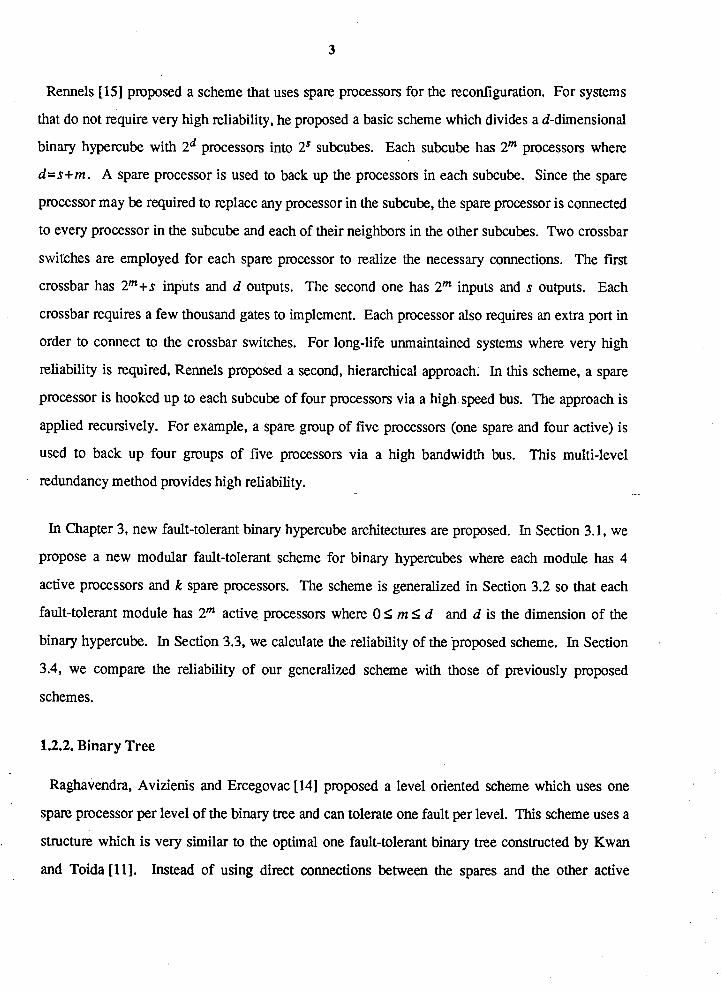
Rennels [15] proposed a scheme that uses spare processors for the reconfiguration. For systems
that do not require very high reliability, he proposed a basic scheme which divides a d-dimensional
binary hypercube with 2d processors into 2S subcubes. Each subcube has 2m processors where
d=s+m. A spare processor is used to back up the processors in each subcube. Since the spare
processor may be required to replace any processor in the subcube, the spare processor is connected
to every processor in the subcube and each of their neighbors in the other subcubes. Two crossbar
switches are employed for each spare processor to realize the necessary connections. The first
crossbar has 2m+s inputs and d outputs. The second one has 2m inputs and s outputs. Each
crossbar requires a few thousand gates to implement. Each processor also requires an extra port in
order to connect to the crossbar switches. For long-life unmaintained systems where very high
reliability is required, Rennels proposed a second, hierarchical approach. In this scheme, a spare
processor is hooked up to each subcube of four processors via a high speed bus. The approach is
applied recursively. For example, a spare group of five processors (one spare and four active) is
used to back up four groups of five processors via a high bandwidth bus. This multi-level
redundancy method provides high reliability. -
In Chapter 3, new fault-tolerant binary hypercube zchitecmres are p r ~ p s e d . h Section 3.1, we
propose a new modular fault-tolerant scheme for binary hypercubes where each module has 4
active processors and k spare processors. The scheme is generalized in Section 3.2 so that each
fault-tolerant module has 2m active processors where 0 I m I d and d is the dimension of the
binary hypercube. In Section 3.3, we calculate the reliability of the proposed scheme. In Section
3.4, we compare the reliability of our generalized scheme with those of previously proposed
schemes.
1.2.2. Binary Tree
Raghavendra, Avizienis and Ercegovac [14] proposed a level oriented scheme which uses one
spare processor per level of the binary tree and can tolerate one fault per level. This scheme uses a
structure which is very similar to the optimal one fault-tolerant binary tree constructed by Kwan
and Toida [ll] . Instead of using direct connections between the spares and the other active

processors, they use two decoupling networks as switches to provide the appropriate connections.
The lower levels of a large tree will have many nodes. In order to increase the reliability of the
lower levels, this level oriented scheme can be applied to modules consisting of k=2' nodes of a
given level. A single spare is provided for each module and the switches in the decoupling
networks are controlled centrally through a host computer that uses the binary tree.
Hassan and Agarwal[7] also proposed a modular scheme for fault-tolerant binary trees. Their
approach uses fault-tolerant modules as building blocks to construct a complete binary tree. Each
fault-tolerant module consists of four processors, three active and one spare. Soft switches provide
connections between the active processors, the spare, and the rest of the tree. A distributed
approach to reconfiguration is used in that the soft switches can be set locally in each module when
failure occurs.
Both the level oriented scheme (with or without modules at the lower level) and the modular
approach provide only one spare per level (or module). Thus, the reliability that can be achieved
by these schemes is insufficient for systems requiring very high reliability. Singh [16] suggested
an improvement to Hassan and Agarwal's modular scheme by allowing the sharing of spares across
module boundaries and allowing more than one spare per module. He showed that his scheme is
best suited for binary trees having 31 to 255 nodes.
For larger binary trees, Howells and Agarwal[9] devised a modular scheme that allows more than
one spare per module. Each module in their scheme is a subtree. For example, a 10-level binary
tree may be split into one 5-level subtree containing the root and 32 5-level subtrees. Each non-
root subtree is a fault-tolerant module with its own spares. Each spare in a module may replace any
active processor in the entire module. Each spare is connected to every processor in the subtree
through direct links to each processor, soft switches, and three buses. Two of these buses are used
to connect to the children of the processor being replaced and the last bus is used to connect to the
parent. This technique cannot be used for the subtree containing the root node since its leaf nodes
must be connected to the root nodes of the other fault-tolerant non-root subtrees. Fortunately, the
subtree containing the root node can employ other schemes to provide fault-tolerance. Besides

improving reliability, both Singh's and Howells and Agarwal's schemes also improve the yield for
binary trees implemented in a single chip.
Lowrie and Fuchs 1121 also proposed a subtree oriented fault-tolerance (SOFT) scheme which
they show to be better than the schemes of Raghavendra, Avizienis and Ercegovac and of Hassan
and Agarwal. In their scheme, up to 2' spares, where 0 I t 5 d-2, are connected to the leaf nodes
of a d-level binary tree. The number of connections between a spare and the leaf nodes depends on
t. An extra link is also used to connect the two children of a non-leaf node together. When a node
becomes faulty, one of its children, s, will take over its task through the use of soft switches. The
task of s will be taken over in turn by one of its children. This process is repeated until a spare
takes over the task of a leaf node. The subtree oriented fault-tolerance scheme can also be
extended to an m-ary tree.
Chapter 4 concentrates on the binary tree architecture. In Section 4.2, we propose a new scheme
for binary trees which is extended in Section 4.3 for m-ary trees. In Section 4.4, we compare the
reliability and hardware costs of our proposed scheme with those of previous schemes. In Section
4.5, we compare both the reliability and hardware costs of variants of our scheme.
1.2.3. Cube-Connected Cycles
Cube-connected cycles, proposed by Preparata and Vuillemin [13], consist of n=h2d processors
with h 2 d . This structure is easily obtained by replacing each vertex of an d-dimensional binary
hypercube with a cycle of h processors, distributing the d edges incident on each vertex of the
hypercube among the vertices of the corresponding h cycles. Figure 1-2 shows a cube connected
cycle with h=4 and d=2.
Banerjee, Kuo and Fuchs [2], and Banerjee [3] proposed two fault-tolerant schemes for cube-
connected cycles. The basic scheme uses one redundant cycle to back up all of the cycles in the
network. In this scheme, an extra port is required for every processor in order to connect the spare
cycle to the rest of the network. For systems requiring higher reliability, they proposed a modular
scheme which provides spares for each cycle and uses a local reconfiguration scheme to tolerate
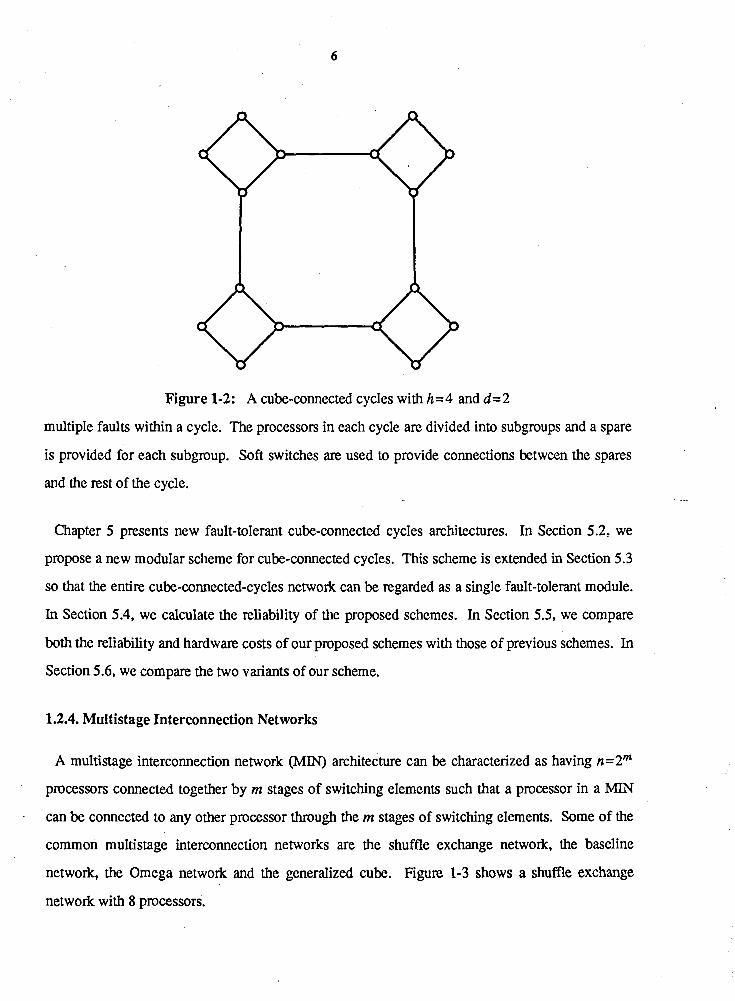
Figure 1-2: A cube-connected cycles with h=4 and d=2
multiple faults within a cycle. The processors in each cycle are divided into subgroups and a spare
is provided for each subgroup. Soft switches are used to provide connections between the spares
and the rest of the cycle. .
Chapter 5 presents new fault-tolerant cube-connected cycles architectures. In Section 5.2, we
propose a new modular scheme for cube-connected cycles. This scheme is extended in Section 5.3
so that the entire cube-connected-cycles network can be regarded as a single fault-tolerant module.
In Section 5.4, we calculate the reliability of the proposed schemes. In Section 5.5, we compare
both the reliability and hardware costs of our proposed schemes with those of previous schemes. In
Section 5.6, we compare the two variants of our scheme.
1.2.4. Multistage Interconnection Networks
A multistage interconnection network (MIN) architecture can be characterized as having n=2m
processors connected together by m stages of switching elements such that a processor in a MIN
can be connected to any other processor through the m stages of switching elements. Some of the
common multistage interconnection networks are the shuffle exchange network, the baseline
network, the Omega network and the generalized cube. Figure 1-3 shows a shuffle exchange
network with 8 processors.

switching elements
stage 0 stage 1 stage 2
Figure 1-3: A shuffle exchange network with 8 processors
Most previous work (see [1]) in the area of fault-tolerant multistage interconnection network
architectures has been based on increasing the reliability of the network connections, Ignoring
processing element failures and concentrating only on the switching element failures. For systems
with a large number of processing elements, it is also important to consider processing element
failures in order to achieve high reliability for the entire system. Jeng and Siegel [lo] proposed a
fault-tolerant multistage interconnection network architecture called the Dynamic Redundant (DR)
network that can tolerate processing element failures as well as switching element failures by using
spare processors and switches. The DR network is based on a generalized cube network. A
generalized cube network with n=Zm processors uses log2n stages where each stage consists of n
switching elements connected by n links to the previous stage. The DR network with n active
processors and k spares has the same number of stages, however each stage has n + k switching
elements rather than n. Each stage is connected to the previous stage using 3(n+k) links. A DR
network can tolerate any single processor failure or any single switching element failure. It can, in
fact, tolerate k faults provided that the faults all occur in adjacent rows. Jeng and Siegel show that

a DR network with more than one spare is no better than a DR network with one spare due to the
limited coverage on multiple faults.
In Chapter 6, new multistage interconnection network architectures are proposed. In Section 6.2,
we propose a new fault-tolerant scheme for multistage interconnection networks with k spare
processors which can tolerate any k processor failures. In Section 6.3, we compare our scheme
with Jeng and Siegel's DR scheme. The scheme is extended in Section 6.4 so that it can cover both
processor failures and switching element failures. In Section 6.5, the extended scheme is compared
to Jeng and Siegel's DR scheme. In Section 6.6, we compare the reliability and hardware
requirements of two variants of the extended scheme.

A General Fault-Tolerant Scheme for Multi-Computer Networks
2.1. Introduction
Our goal is to provide fault-tolerance in a multi-computer network by adding spare processors
which can be used to replace failed processors. In particular, we want to design a method to
connect spare processors to an existing network in such a way that the network topology can be
maintained when a spare processor replaces a failed processor. One obvious approach is to connect
each spare to a l l the processors in the network using large cross-bar switches. This is not feasible
for large networks. In order to overcome this problem, the entire network can be divided into
modules such that each spare is used to back up the processors within a particular module. The
fault-tolerant modules are then connected together to form the network Since a spare c m be used
to back up any processor in the module which may be connected to processors outside of the
module, the spare must be able to connect to those external processors. These connections may be
realized with smaller cross-bar switches. Although large cross-bar switches are not needed in this
scheme, the number of spares required to provide the same level of system reliability increases as
the number of processors in a module decreases. Thus, there is a trade off between the module size
and the size of the cross-bar switches required by this approach.
Rather than using spares to back up an entire module, we can use the spares to back up only a
very small number of processors. These processors, in turn, can be used to back up other active
. processors in the module. This process can be repeated until every processor is backed up. With
this approach, cross-bar switches can be avoided entirely.
We propose a new interconnection method in Section 2.2 which uses switching networks instead

of cross-bar switches to connect fault-tolerant modules together. These networks can also be used
to provide connections within a module. The approach can also be used so that the entire network
is realized as a single fault-tolerant module. In Section 2.3, reliability estimates for our schemes
are given. The switching networks used in our interconnection method are described in Sections
2.4 and 2.5. Finally, a distributed reconfiguration scheme is given in Section 2.6.
2.2. Using Switching Networks to Construct Fault-Tolerant Networks
In constructing fault-tolerant networks, we will require a switching network with n incoming and
n+ k outgoing links as shown in Figure 2-1. In particular, let a l , %, ..., an be a sequence such that
1 I al < < ... < an I n + k . We want to design a switching network which allows the n
incoming links to be connected to any such sequence a l , %, ..., a, of outgoing links so that
incoming link i is connected to outgoing link $. The detailed design of such switching networks is
described in Sections 2.4 and 2.5.
n incoming links
n+k outgoing links
Figure 2-1: A switching network with n incoming links and n+ k outgoing links
In describing the construction of fault-tolerant networks, we use the term active processor to
denote all the processors that participate in the execution of tasks.
Let us, for the moment, assume that we can construct a fault-tolerant module with n active
processors and k spare processors which functions correctly provided that no more than k
processors fail within the module. Consider a network consisting of two fault-tolerant modules.

module 1
module 2
Conceptual network - 6 processors in module 1 connected to 6 processors in module 2
I switching network I
I switching network
I I I I
fault-tolerant network - 6 active processors in module 1 connected to 6 active processors in module 2
Figure 2-2: Using switching networks to connect two fault-tolerant modules
Each module initially contains 6 active processors (numbered 1 through 6) and one spare processor
(numbered 7) and the i h active processors of each module are connected by a link. We now
describe how to connect one module to the other using switching networks. Let al , $, ..., a6 be
the numbers of the active processors in a module, ordered so that 1 I al < % < ... < a6 I 7.
Incoming links 1, 2, 3, ..., 6 can be routed to any such sequence of processors al, %, ..., a6,
respectively by using a switching network with 6 incoming links and 7 outgoing links (see Figure
2-2). Each outgoing link of the switching network is connected to a processor in the module. Each
incoming link is connected to a communication line that leads to the other module. Initially, these
6 communication lines are connected to processors 1 through 6. When one of these processors

fails, the switching network resets the connections so that the failed processor is disconnected and
the 6 communication lines are routed to 6 non-faulty processors. For example, if processor 5 fails,
processor 6 will be connected to communication line 5 and the spare processor (7) will be
connected to communication line 6 . In this simple example, each processor is connected to only
one processor in another module. Additional switching networks could be utilized to allow
multiple external connections.
Figure 2-3: Using direct connection to construct a fault-tolerant cycle of six processors
Now, we turn our attention to the connections within a given fault-tolerant module. Continuing
with our example, we would like to construct a fault-tolerant 6 cycle. In particular, the 6 initially
active processors must fonn a cycle by connecting processor i to processor i+ 1, for 1 I i < 6 and
processor 6 to processor 1. The fault-tolerant module is designed so that processor i (1 I i I 6) is
"backed up" by processor i+ 1. That is, if processor i fails (or is called upon to replace yet another
processor) then processor i+ 1 can replace processor i. To allow for these processors to replace
each other in the event of a failure, additional connections must be added. One method to do this,
which we call direct connection, is to connect processor i to i+2 for 1 5 i I 5 and processor 7 to
processors 1 ,2 and 6 (see Figure 2-3). One drawback of this method is that the number of ports per
. processor must increase with the number of spares. A second method is to use two cross-bar
switches to connect the spare processor(s) to the cycle. As the number of spares becomes large,
this method also becomes infeasible. A third approach which uses switching networks does not
require the number of ports to increase with the number of spares and is described below.

The connections between the processors in a module can be provided by connecting the incoming
links of several groups of switching network. In our particular example, the connections between
the processors within a module can be provided by two switching networks with 6 "incoming" and
7 "outgoing" links. In this case, the 7 processors of the module are connected to the "outgoing"
links while the "incoming" links are connected to each other. One switching network is used to
connect processor i to processor i+ 1 for 1 I i 5 6 where i is odd. The second connects processor i
to processor i+ 1 for 1 I i 5 5 where i is even and processor 6 to processor 1. With these
connections, the processors connected to the 6 "incoming" links form a cycle of six processors.
The connections are shown in Figure 2-4. If processor 5 fails, processor 6 will take over the task of
faulty processor 5 and the spare processor 7 will take over the task of processor 6. The switching
networks can be set to bypass processor 5. In particular, "incoming" links 5 and 6 are reset to
connect to "outgoing" links 6 and 7, disconnecting "outgoing" link 5. The details of this process
are explained in Sections 2.4 and 2.5. After reseting the switching network, processors 1,2,3,4,6,
and 7 form a cycle of six processors, connected through the switching networks. This same
technique can be used to form different structures within the module as illustrated in Chapters 3,4,
5, and 6.
I I 1 I I I I switching network switching network
Figure 2-4: Connecting a cycle with 6 active processors and 1 spare processor using two switching networks
By using switching networks to provide connections between processors within a module and

connections between modules, a fault-tolerant multi-computer network can be constructed as
described above. We call this scheme modular sparing. In the above example, each spare can be
used to replace any of 6 processors within its own module. Thus, the system can tolerate any single
failure. It can also tolerate two failures if they occur in different modules. In order to tolerate any
two failures in the network, we could use the above techniques to construct a single module
containing 12 active processors (divided into 2 cycles of 6 processors each) and 2 spare processors.
We call this scheme global sparing.
As an example of global sparing, we show in Figure 2-5 an alternate implementation of the above
example. As before, we want 2 cycles of 6 active processors and we allow 2 spare processors.
Three switching networks are required to provide the connections. The first two switching
networks are used to connect the processors to form two cycles of six processors using the same
connection scheme as described above for providing connections for a cycle of six processors. The
processors connected to "incoming" links 1 to 6 and 7 to 12 of both switching networks form two
cycles of six processors respectively. Finally, the third switching network is used to connect the
two cycles together.
Using global sparing, k spares in the network can tolerate any k faults. Thus, it is optimal in the
number of faults that any network with a given number of spares can tolerate. With global sparing,
it is possible to achieve the same level of reliability as with modular sparing and other proposed
schemes for various multi-computer network architectures as shown in Chapters 3, 4, 5, and 6
while using significantly fewer spares. However, for networks with a large number of active
processors, it may not be possible to implement the entire network on a single wafer. Smaller
modules may be used to split a large network into fault-tolerant modules which can each be
implemented on a wafer.

I switching network I
connect to processors as numbered
I switching network I
I I
switching network 1
Figure 2-5: Connecting a network with two cycles of six processors and two spare processors using three switching networks
2.3. Estimation of the Reliability of the Scheme
Consider a fault-tolerant multi-computer network c o n ~ t ~ c t e d using global sparing which contains
n active processors and k spares. In our reliability analysis, we consider only processor failure. We
do not consider the failures in the switching networks. These failures could be covered by
duplicating the switching networks. Other types of failures, such as fault-detection failures and
recovery failures, are accounted for by the coverage factor [l7] which is defined to be the
probability that a failure is detected and the recovery is successful. If reconfiguration fails due to
one of these failure types, the entire system is considered to be unreconfigurable.
Let c be the coverage factor, k the number of spare processors in the network, n the number of

active processors in the network, r= cXt the reliability of a single processor (where is a constant
representing the failure rate of a processor over time t and t is time expressed in millions of hours),
and Rk the reliability of a fault-tolerant network with k spare processors using global sparing. The
reliability of a non-redundant network Ro is rn. For k= 1, the probability that the spare is needed is
equal to the probability that an initially active processor has failed which is (;) rn-' (1 -r). The
probability that a particular spare processor is reliable and can be switched successfully is rc.
Thus, the additional reliability with one spare is rc(;)rn-'(1-r) and the reliability R1 is
R1 = rn+(;)rn(l-r)c= R0+(;)rn(l-r)c. For k=2, the second spare is only used when there
are exactly two faulty processors among the n initial active processors and the first spare. The
probability that this occurs is (";'I rn-I (1-r12c. Thus, the reliability with two spares is
R2 = ~ ~ + ( ~ ; l ) r " ( l - r ) ~ c ~ ,
For arbitrary k,
.-
The reliability of a network using modular sparing can be calculated similarly. Let m be the
number of active processors in each module, be the reliability of a module with k spares in
each module, and Rp,m,k be the reliability of a network with p modules each having m active
processors and k spares.
2.4. Type A Switching Network Design
A Type A switching network can be implemented using a group of decoupling networks. The
group of decoupling networks maps n incoming links (numbered 1 to n) to n+ k outgoing links
(numbered 1 to n+ k). Each outgoing link is connected to a processor. The use of decoupling
networks has previously been proposed for other fault-tolerant multi-computer network
architectures [14,4,5,6]. Figure 2-6 shows the connections for a group of 3 decouplig networks
arranged in three levels as a Type A switching network.

incoming links
level 2
level 1
level 0
processors
Figure 2-6: 3 decoupling networks arranged in 3 levels
The levels of each group of decoupling networks are numbered from 0 to 1-1 with level 0
connecting to the outgoing links and level 1-1 connecting to the incoming links. Each level
contains at most n+k-1 switches numbered from 1 to n+k- 1. The j th switch in level 1- 1
connects to the j b incoming link. It can be set to connect the j th incoming link te either the j th
switch on level 1-2 or to the (j+ switch on level 1-2. In general, the j th switch on the i th
level can be set so that it is connected to either the j th switch on level i- 1 or to the (j+ switch
on level i- 1. The j th switch on level 0 can connect to either the j th outgoing link or the (j+
outgoing link. Initially, every switch j on level i > 0 is set to connect to switch j on level i- 1.
Switch j on level 0 is initially set to connect to outgoing link j.
Outgoing link i is connected to processor i. At any given time, n processors are active. We
denote the active processors as al , ..., an with al < % c ... < an such that al is the number of the
. lowest numbered active processor and an is the number of the highest numbered active processor.
. In particular, ai= j indicates that processor j is the i rh active processor.
When a processor fails, the failed processor has to be disconnected from the network and the
spare has to be connected. As an example of the reconfiguration process, consider a module with 8

active processors and 3 spare processors. If processor 3 fails, the switch in level 0 of the
decoupling network that connects to processor 3 and all the switches to the right of it are switched
to the right. In this way, processor 3 is disconnected and the first spare processor (9) is activated.
Processor i+ 1 assumes processor i's previous role where 3 5 i 4 8. At this point, al = 1, %=2,
and ai= i+ 1 , for 3 4 i I 8 . The new connection for one group of decoupliig networks is shown in
Figure 2-7. If another processor fails subsequently, another reconfiguration must occur. The
switch in level 1 of the decoupling network that connects to the failed processor and all the
switches to the right of it are switched to the right. Figure 2-8 shows the structure as further
modified after processor 1 becomes faulty and is replaced. In this figure, a1 =2, and ai=i+2, for
2 I i < 8. Finally, Figure 2-9 shows the result of processor 7 failing subsequently and is replaced.
Afterreconfiguration,al=2,%=4,0[3=5, a4=6, andai=i+3, for51 i I 8.
incoming links
level 2
levd i
level 0
Figure 2-7: Connections after processor 3 has failed
Consider one such k level decoupling network connected to n active processors and k spares. Let
i be the number of processors that have failed previously, where 0 I i I k. If another active
processor fails, the reconfiguring is done by switching the switch in level i that connects to the
failed processor and all switches of the same level to the right of it one position to the right. For
example, if the switches in level i are numbered 1 to n+k-i-1 from left to right and switch j

incoming links
level 2
level 1
level 0
Figure 2-8: Connections after processor 1 and 3 have failed
incoming links
level 2
level 1
level 0
Figure 2-9: Connections after processor 1 .3 and 7 have failed
connects to the newly failed processor, then the reconfiguration consists of switching the switches
from j to n+k- i - 1 at level i to the right. By doing so, the faulty processor is disconnected from
the network, the spare processor immediately to the right of the rightmost active processor becomes
an active processor, and the structure is reestablished.

A Type A switching network consists of k decoupling network arranged in k levels. Incoming
link i can be connected to any outgoing link j if j- i I k as shown in Lemma 1. Lemma 1 and other
subsequent Lemmas described below are used to establish that a Type A switching network can be
used to replace up to k faulty processors with spares.
Lemma 1: In a Type A switching network, incoming link i (1 l i l n) can be
connected to any outgoing link j where (i I j 5 i+ k)
Proof: Let m=j-i . At each level 1, 0 5 1 5 m, set switch number i+m-1-1 and all
switches in that level to the right of switch i+m-1-1 to the right. This connects
incoming link i to outgoing link j. 0
Let a l , a,?, ..., an be a sequence such that 1 I al < a,? < ... < an 5 n+k. If the n incoming links
can be connected to any such sequence al, a,?, ..., an of outgoing links so that incoming link i is
connected to outgoing link 04- for 0 < i I n , a Type A switching network can be used to replace any
group of up to k faulty processors with spares. In order to show that this is the case, we first prove
Lemma 2 which shows that a Type A switching network can be used to connect incoming links i
and p (p > i) to outgoing links j and q (q > j, q-p 2 j-i) , respectively so that the paths do not
intersect.
Lemma 2: In a Type A switching network, if incoming link i is connected to outgoing
link j and incoming link p (p > i ) is connected to outgoing link q (q > J] , and q-p 1 j-i,
the switches used to connect i to j, and the switches used to connect p to q are all
different.
Proof: Let sl be the switch used in level 1 to connect i to j and let tl be the switch used
in level 1 to connect p to q. Since p > i , in level k- 1 , tk- > sk- l . If sk- is switched to
the right, then tk- is also switched due to the reconfiguration scheme. Thus, in level
k-2, tk-2 > s ~ - ~ . The same argument can be repeated until level 0 is reached. Hence,
t l>sl fo r05 IS k-1.
Theorem 3: Let a l , %, ..., an be a sequence such that 1 I al c < ... < an l n+ k.
The n incoming links of a Type A switching network can be connected to any such

sequence a l , a,?, ..., a, of outgoing links so that incoming link i is connected to outgoing
linka,forOI i I n .
Proof: From Lemma 1, incoming link i can be connected to ai for 1 I i l n. From
Lemma 2, there will be no common switch used to connect incoming link i to outgoing
link ai and incoming link i + 1 to outgoing link ai+l for 1 5 i S n-1 . Thus, the
theorem is proved.
For a Type A switching network with n incoming links and n + k outgoing links, a level i
decoupling network must have n+k- i - 1 switches. Thus, a Type A switching network has a total k of xj- - (n+ k-0 = k(2 n+ k- 1)/2 switches. For large k, the number of switches required for a
Type A switching network increases rapidly. The hardware required to implement the switches
may make this design infeasible. Furthermore, k levels of decoupling networks are used to add k
spares. When k is large, the switching delay may be significant. Hence, a Type A switching
network is not suitable when k is large. The next section presents a different design which requires
a lot fewer switches and introduces less switching delays when k is large. However, when k is
small, the simplicity of a Type A switching network makes it easier to implement than other more
complicated designs.
2.5. Type B Switching Network Design
For large k, we propose a different switching network design called Type B that uses fewer
decoupling networks and switches than Type A. Instead of allowing the j switch of level i to be
c o ~ e c t e d to the j switch or the (j+ switch of level i- 1, the j h switch of level i may be
connected to the j or the (j+2')& switch of level i- 1. The j th switch on level 0 can connect to
either the j th outgoing link or the (j+ outgoing link. Initially, every switch j on level i > 0 is
set to connect to switch j on level i - 1 . Switch j on level 0 is initially set to connect to outgoing
. link j. With this design, only I = r1og2(k+ 111 levels of decoupling networks are required to
incorporate k spares.
The reconfiguring process of this design is slightly more complicated than for Type A. Consider
one such 1 level decoupling network connected to n active processors and k spares. As before, we
number the levels from 0 to I- 1, the processors from 1 to n+k, and the active processors from orl
to an. ai=j indicates processor j is the i th active processor. Initially ai=i for 1 I i I n. When
the first active processor fails, the reconfiguration process is the same as for Type A. The switch in
level 0 that is connected to the failed processor and all the switches to the right of it are switched
one position to the right. However, when subsequent failures occur, each remaining active
processor and the spares used to replace the failed processors must determine which switches to
use.
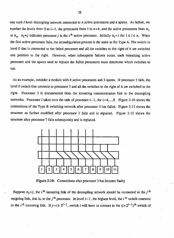
As an example, consider a module with 8 active processors and 3 spares. If processor 3 fails, the
level 0 switch that connects to processor 3 and all the switches to the right of it are switched to the
right. Processor 3 is disconnected from the incoming communication link to the decoupling
networks. Processor i takes over the task of processor i-1 , for i=4, ... ,9. Figure 2-10 shows the
connections of the Type B switching network after processor 3 has failed. Figure 2-1 1 shows the
structure as further modified after processor 1 fails and is replaced. Figure 2-12 shows the ,-
structure after processor 7 fails subsequentlyand is replaced.
Figure 2-10: Connections after processor 3 has become faulty
. Suppose a i=j , the i th incoming link of the decoupling network should be connected to the jh
outgoing lid, that is, to the j h processor. In level 1-1, the highest level, the i th switch connects
to the i incoming link. If j-i 2 2lv1, switch i will have to connect to the (i+21-1)th switch of

Figure 2-11: Connections after processor 3 and 7 have become faulty
Figure 2-12: Connections after processor 1,3 and 7 have become faulty
level 1-2. Otherwise, no change is required and it remains connected to the i fh switch of level
1- 1. ~ e t j - i = ~ k : ~ a,,,2m where am is either 0 or 1 and I = rlog2(k+ 1)l. If j-i 2 2'-l, al- = 1 .
Otherwise, al-l=O. For level 1-2, the switch used in the connection from incoming link i to
processor j depends on whether the switch used in level 1- 1 is switched or not. This information
can be obtained from the value of ale If a[- = 1 , the (i+2'-I)& switch is used. Otherwise, the
i" one is used. That is, the switch used in level 1-2 is the (i+a1-121-1)m switch. This switch is
switched to connect to the (i+al- 121-1 +2lq2)" switch in level 1-3 if (1-0-a1-12'-1 2 2'-'.
. That is, if al-2= 1. Otherwise, switching is not necessary. Hence, the switches used in the
connection and the status &the switches used can be obtained from the equation j - i = ~ ! & am2m
with al=O to simplify the formulas below. In particular, i + ~ : = , + ~ ~ 2 ~ 2 ~ switch in level u is

used to connect incoming link i to outgoing link j of the decoupling network. This switch is set to I connect to the (i+ xm- - am2m)" switch of level u- 1 (or the (i+ x:, , am2m)" outgoing link if
u=O). With this switching scheme, the n incoming links of the i=rlog2(k+l)l levels of
decoupling networks can be connected to n non-faulty processors if the number of faulty processors
is less than or equal to k. Furthermore, no two connections between an incoming Sink and an active
processor share a common S i or common switch.
In order to prove that the rlog2(k+ 1)1 levels of decoupling networks can be configured to handle
any k processor faults, let al, %, ..., a, be a sequence such that 1 I al < 9 < ... < a, l n+k. If
the n incoming S i s can be connected to any such sequence al, 9 , ..., a, of outgoing links such
that incoming link i is connected to outgoing link ai for 0 I i I n, a Type B switching network can
be used to replace any of up to k faulty processors with spares. In particular, incoming link i must
be able to connect to any outgoing link j in the range i I j I i+k. This is proved in Lemma 4
below.
Lemma 4: In a Type B switching network incoming link i (1 I i S n) can be connected &
to outgoing link j for any j where i I j I i+ k.
Proof: Since i S j 5 i + k and xLi0 2m 212 k , j- i can be expressed as ~ l - 1 U-o a u 2U, where
the a's are either 0 or 1 and c:.~ - Zrn 2 x::: ap". Using the connection scheme
described above, incoming link i to the decoupling network is connected to outgoing link
j = i + 2 Since i+ C~I: - a? I i+ x L ~ ~ zrn, incoming link i can be connected
to outgoing link j. 0
Lemmas 5 and 6 establish that if any incoming link i is connected to outgoing link j, where
i l j I i+k, incoming link i+ 1 must be able to connect to any outgoing link t in the range
j + l I t S i+k+l with no sharing of switches and no sharing of links between these two
connections. Lemma 5 is a technical lemma useful in proving Lemma 6.
I I I Lemma 5: If ~rn-sam2m>~mC,=sbrn2m - then ~ ~ - ~ a ~ 2 ~ - ~ ~ = ~ b ~ 2 ~ ~ - 2s where
the a's and b's are either 0 or 1.

Proof: Let 1' be the largest value 1 2 2' 2 s such that a p by. Since we have assumed I that xm=sam2m > EL=, bm2m and all the a's and b's are either 0 or 1, it must be the
r-1 Since Ern=, am2" 2 0 and - bm2m 5 2s-2s,
Y am2m-~m=, bm2rn 2 P. o
Lemma 6: For a Type B switching network, if incoming link i is connected to outgoing
link j and incoming link p @ > i) is connected to outgoing link q, where q > j
(q-p 2 j- i), the switches used to connect i to j, and the switches used to connect p to q
are all different.
Proof: Let j-i=;~:k-!~ bm2m and q-p=~k,-fo amZm, where the a's and b's are either 0
I- 1 or 1 and l= rlog2k+ 11. Thus, z;io a,Zm-2 Em=o bm2m. At each level s, the
connection fmm i to j utilizes switch i+c.kJs bm2" while the connection from p to q
uses switch + am2m. These switches are clearly distinct if
Suppose that for a particular s, ~ ~ ~ ~ b , 2 ~ > ~ ~ ~ ~ a ~ 2 ~ . Since,
p - 1 1-1 m.O amZm 2 zmZO bm2m. therefore,
ES- 1 I-' b 2m-z1-1 a 2m. zs-l a 2 m - ~ s - 1 b 2m>zm=, s- 1 m = ~ m m = ~ m m=s m m=o am2m-xm=o bm2" is
at most equal to xk-=l0 2m=2s- 1. From Lemma 5, xk,-fS - bm2m-~'-1 a 2m is at least m=s m
2S. A contradiction occurs and hence the lemma is proved.
Theorem 7: Let al, q, ..., an be a sequence such that 1 S al c % c ... c an l n+ k.
The n incoming links of a Type B switching network can be connected to any such

sequence al , %, ..., a, of outgoing links such that incoming link i is connected to
outgoing link q for 0 I i 5 n.
Proof: The proof follows from Lemmas 4 and 6. 0
The number of switches required in each level of a Type B switching network depends on n and
k. If processor n+k, the last spare, can be connected to the n th incoming link of the decoupling
networks, the switches in the decoupling networks are sufficient to connect any incoming link i,
1 I i I n, to any outgoing link j, i I j 5 i+k. With this observation, the total number of switches
in a group of decoupling network can be obtained. Let k=x;Jo am2m, where the am's are either 0
or 1 and al- l= 1. The level 1- 1 decoupling network has n switches which are connected to the n
incoming links to the group of decoupling networks. The n th switch can connect to either the n th
switch or the n+2'-l switch in level 1-2. Thus, the number of switches in level 1-2 is
n+al-121-1. The last switch (n+a1-121-1) in level 1-2 is not required to connect to the
n+21-1+21-2 switch in level 1-3 when al-2=0. In this case, not all of the switches have to be
switchable. Figure 2-13 shows an example in which some switches do not have to be switchable. .-
Hence, for level 1-3, the number of switches is n + ~ k L - ~ am2m. Similarly, for level i, the
number of switches is n+zkJi+ a 2m. With this number of switches, the n fh incoming l i i is
able to connect to the last spare processor because k = ~ k ' ~ am2m. Thus, for a Type B switching
network with 1 = rlog2k+ 1 1 levels, the total number of switches is nlc z;il rn~2,2~.
2.6. Distributed Reconfiguration
Consider a module with n active processors and k spare processors. The n+k processors are
connected to the n+k outgoing links of a switching network and are numbered 1 to n+k
corresponding to the numbers of the outgoing links. The active processors are denoted by a i , for
1 5 i 5 n. ai=j indicates that processorj is the i th active processor. Initially, a i= i for 1 5 i < n.
In order to provide fast context switching and distributed reconfiguration, processor i is
connected to processor i+ 1, where 1 5 i 5 n+k- 1, with soft switches used to bypass faulty

non-switchable switches
Figure 2-13: For n=8 and k=4, some switches do not have to be switchable
processors. Figure 2-14 shows the connections and soft switches between the processors. When a
processor is non-faulty, a signal is sent to its switches to keep them open. We assume that the fault
detection of each processor is concurrently performed by means of some on-line self-testing
circuits. Thus, when a proces-spr fails, it stops sending this signal and the processor to its right will
be able to detect the failure and start the reconfiguration process.
Figure 2-14: Connections between the processors
When a processor ai=j fails, the network must be reconfigured to disconnect the faulty
processor, connect a spare one and reassign tasks among the active processors. The non-faulty
active processor ai+ immediately to the right of the faulty one initiates the reconfiguring process
upon detecting that ai has failed. (If i = n , the lowest numbered spare processor m initiates the
. reconfiguration process.) It starts by taking over the task of the faulty one and informs the non-
faulty processor to its right about the starting of the reconfiguring process. Processor ai+ 's task is
then taken over in turn by the non-faulty processor immediately to its right. This process is

repeated until the spare processor m immediately to the right of the rightmost active processor (a,)
becomes an active processor and takes over the task of its predecessor. That is, when processor aj
fails, a sequence of task reassignments are performed until a non-faulty spare processor m which is
connected to the processor a, is activated. First, aj's task is taken over by aj+l and aj+l
becomes active processor aj. This processor's old task is given to aj+2 and orj+, becomes active
processor aj+l. This continues until a, becomes active processor an- Finally, an's old task is
taken over by the spare processor m and m becomes a,.
The reassignment of tasks can be carried out efficiently through the connections between the
processors if a parent-child relationship [18] is assumed between any two neighboring processors.
The processor on the right assumes the role of the parent and keeps track of the state of its child.
When a child fails, its parent can take over its task and can in turn inform its own parent of the
reconfiguring process without any delay or rollback. For example, assuming that n= 8, k=2 and
ai= i, processor 10 is the parent of processor 9 initially and processor 9 is the parent of processor 8
and so on. That is, processor i+ 1 is the parent of processor i initially, for 1 I i I 9. If processor 5
fails, its parent, processor 6, can take over its task easily for processor 6 already has the current
state of processor 5. The new child (processor 4) of processor 6 sends its cumnt state t~ processor
6 and processor 6 informs its parent (processor 7) of the reconfiguration and sends its current state
to its parent. This process is repeated until processor 9 takes over the task of processor 8 and sends
its current state to its parent, processor 10. The above reconfiguring process can be carried out
efficiently using the links between the non-faulty processors. The transfer of state information
between the processors can be done almost simultaneously.
This scheme can only handle either a single fault at a time or multiple faults at the same time if
the faults are not adjacent to each other. For multiple faults not adjacent to each other, the
reassignment process is still quite efficient although the state of more than one processor may be
transferred between the non-faulty processors. If adjacent faults occur simultaneously, the
reassignment of tasks will take more time since the entire system may have to restart at the
previous check point instead of being able to continue its operation without rollback.

After the reassignment of tasks is completed, the switching networks must also be reset as
described in Section 2.4 or Section 2.5 to replace the failed processors with spares. For a Type A
switching network, the control of the decoupling networks can be implemented at each spare
processor. The first spale controls the level 0 decouplimg ne&ork and the i th spare controls the
level i-1 decoupling network. For a Type B switching network, when processor j is required to
take over the task of another processor to its right, it knows which active processor ai it will
become and it also knows its own position. Thus, the values i and j are both known to processor j .
Processor j calculates the coefficientsa, from the equation j - i = ~ k l ~ am2m and determines
which switches are used and which must be switched for the connection. This information is sent
to the decoupling networks to establish the connection from incoming link i to processor j. This
switching scheme can be carried out distributively by each affected processor. After both steps of
the reconfiguration process (reassignment of tasks and reseting the switching network) have been
completed, the network can resume its normal operation.

Chapter 3
Binary Hypercube Architecture
3.1. Introduction
In this chapter, fault-tolerant binary hypercube architectures are proposed. In Section 3.2, a
fault-tolerant biary hypercube architecture is proposed which uses fault-tolerant modules as
building blocks to realize a binary hypercube. The use of fault-tolerant modules has previously
been proposed for use in fault-tolerant binary tree architectures [5 ,7 ,9 , 161. A fault-tolerant
module contains four active processors and k spare processors configured so that each module can
tolerate up to k faults. Let d be the dimension of a binary hypercube. In Section 3.3, we generalize
the scheme so that each fault-tolerant module has 2m active processors, 0 I m S d, and k spare
-- processors. In Section 3.4, we calculate the reliability of the proposed scheme. With m=d, the
entire biary hypercube is a single fault-tolerant module in whish the k spare processors car. k
used to tolerate any k processor failures. In Section 3.5, we show that with this special case, it is
possible to achieve the same level of reliability as with smaller modules while using significantly
fewer spares. We compare this special case with RenneIs' schemes. The new scheme is more
reliable than Rennels' basic scheme since the latter can tolerate only a single fault within a given
module. Even with fewer spare processors, our scheme achieves higher reliability than does
Rennels' hierarchical approach. Furthermore, the amount of extra hardware required for our
scheme to achieve the same level of reliability as Rennels' scheme is much less than that required
by Rennels' scheme.

3.2. Fault-Tolerant Scheme For Binary Hypercubes
A fault-tolerant binary hypercube can be constructed by using a number of fault-tolerant modules.
We assume initially that each fault-tolerant module consists of 4 active processors and k spares,
connected in a cycle to model a 2-dimensional binary hypercube. Since only four processors are
active at any given time within each 2-dimensional binary hypercube, the spare and faulty
processors must be bypassed. This can be done using soft switches in the cycle as shown in Figure
3-1. These 2-dimensional hypercubes are connected together to form a d-dimensional binary
hypercube. An alternative to the use of soft switches within each module is discussed in Section
3.3 along with the generalization of this construction. The connections between the 2-dimensional
binary hypercubes are realized by either a Type A or Type B switching network such that only
those active processors in the 2-dimensional binary hypercubes are connected.
soft switches
Figure 3-1: A fault-tolerant module with k spares
For a d-dimensional binary hypercube, d-2 groups of switching networks are required for each
2-dimensional hypercube in the network. A group of switching networks is used for each
dimension beyond the second dimension. The first group is used to connect a 2-dimensional binary
hypercube to another 2-dimensional binary hypercube to form a 3-dimensional binary hypercube.
The second group for each 2-dimensional hypercube in a 3-dimensional hypercube is used to
connect to a 2-dimensional hypercube in another 3-dimensional hypercube, forming a 4-
dimensional hypercube. Similarly, the i th (1 I i I d-2) group for each 2-dimensional hypercube
in an i+ 1-dimensional hypercube is used to connect to a 2-dimensional hypercube in another
i+ 1 -dimensional hypercube, forming an i+2-dimensional hypercube. Hence, a d-dimensional
binary hypercube can be formed using 2d-2 2-dimensional hypercubes and 2d-2(d-2) switching
networks.

When a processor fails, the fault-tolerant module must be reconfigured to disconnect the faulty
processor, connect a spare one, and reassign tasks among the active processors. The reconfiguring
process is as described in Chapter 2. In addition, the faulty processor must also be disconnected
from the cycle of active processors in its fault-tolerant module while the spare processor
immediately to the right of the rightmost active processor becomes an active processor and is
connected to the cycle of active processors. This is done using soft switches. The structure of the
2-dimensional binary hypercube is now re-established. After the restructuring has been completed,
the processor immediately to the right of the faulty one in the cycle of active processors, takes over
the task of the faulty one. This processor's task will be taken over in turn by the active processor
immediately to its right. This process is repeated until the newly activated processor takes over the
task of its predecessor. At this point, the reconfiguration is completed and the binary hypercube
can resume its regular operation.
As an example of the reconfiguration process, consider a fault-tolerant module with 3 spare
processors in a 3-dimensional binary hypercube as shown in Figures 3-2 through 3-4. If processor
3 fails, the switch of level 0 that connects to processor 3 and a l l the switches to the right of it are
switched to the right. Processor 3 is disconnected from the cycle of active processors and the fist
spare processor (5) is added to it. Processor 4 assumes processor 3's previous role in the cycle and
processor 5 takes the previous role of processor 4. The new connections are shown in Figure 3-2.
Figure 3.3 shows the structure as further modified after processor 1 fails and is replaced. Figure
3.4 shows the result of processor 5 subsequently failing and being replaced.
3.3. Generalized Scheme for Binary Hypercubes
The scheme described in Section 3.2 has four active processors in each fault-tolerant module.
With minor modifications to the scheme, the number of active processors in a fault-tolerant module
can be any value 2m where d 2 m 2 0.
In Section 3.2, we showed how to use Type A or Type B switching networks to connect one
module of four active processors and k spares to another. The same technique can be used to

level 2
level 1
level 0
Figure 3-2: Connections after processor 3 has become faulty
level 2 rtttt? level 1
I I I I I I level 0 0 c
Figure 3-3: Connections after processor 1 has become faulty
connect modules with different numbers of active processors. In fact, a Type A or Type B
switching network can be used to connect a module of 2m active processors and k spares to another
identical module for any m 2 0 and m -< d, provided that the number of incoming communication
links in the switching network is 2m. Thus, if we can build fault-tolerant modules with 2m active
processors, we can connect them together as described in Section 3.2 to form a d-dimensional
binary hypercube.

level 2
level 1
level 0
Figure 3-4: Connections after processor 5 has become faulty
In addition to these connections between modules, the processors of each module are also
connected together. In particular, in Section 3.2, four active processors and k spares are connected
in a cycle to model a Zdimensional binary hypercube with soft switches being used to bypass both
faulty and spare processors. These soft switches can be replaced by two groups of either Type A or
Type B switching networks. Figure 3-5 shows how to use two Type A switching networks to
connect four active processon and one spare in a fault-tolerant 2-dimensional binary hypercube.
1 2 3 4 5 1 2 3 4 5 connect to processors as numbered
Figure 3-5: Using 2 Type A switching networks to form a fault-tolerant 2-dimensional binary hypercube
The first group is used to connect two neighboring active processors to form two 1-dimensional
binary hypercubes. This is done by connecting the lSt and 2nd. and the 3" and 4& incoming
communication links of a Type A or Type B switching network. The second group is used to
connect these 1-dimensional binary hypercubes to form a Zdimensional binary hypercube by

connecting the IS' incoming communication link to the 3rd and connecting the 2"d to the 4". This
scheme can be extended to modules with more than four active processors or with more than one
spare. For example, a module with eight active processors and k spares can be built by using three
groups of either Type A or Type B switching networks. Figure 3-6 shows how to use three Type A
switching networks to construct a fault-tolerant 3-dimensional binary hypercube with eight active
processors and one spare. The first group is used to connect pairs of processors together to form
1--1
1 2 3 4 5 6 7 8 9 connect to processors as numbered
Figure 3-6: Using 3 Type A switching networks to form a fault-tolerant 3-dimensional binary hypercube
1-dimensional binary hypercubes. This can be done by connecting the lSt and 2nd, 3rd and 4h, 5"
and 6&, and the 7' and 8& incoming links of the fim group of Type A switching network. The
four 1-dimensional binary hypercubes formed are then connected in pairs, creating two 2-
dimensional binary hypercubes using the second group of Type A switching networks. This is
done by connecting the lSt and 3rd, 2nd and 4&, 5h and 7&, and the 6" and 8& incoming links to
form two 2-dimensional binary hypercubes. Finally, the lSt and 5&, 2nd and 6h, 3rd and 7&, and
the 4& and 8" incoming links for the third group are connected to form a 3-dimensional binary
hypercube. With the three groups of Type A switching networks, a fault-tolerant module with 8
active processors can be built.

36
The group of switching networks used to connect pairs of processors together to form 1-
dimensional binary hypercubes can be replaced by connecting processor i to i + l , where
1 I i < n+k-1 and n=2d. Initially, the 1-dimensional binary hypercubes are formed by the
connection between processor 1 and 2, processor 3 and 4, processor 5 and 6, and processor 7 and 8.
When a processor fails, it is bypassed using soft switches. The 1-dimensional binary hypercubes
are then formed by the pairs of connected non-faulty processors. For example, if processor 6 has
failed, the 1-dimensional binary hypercubes are processor 1 and 2, processor 3 and 4, processor 5
and 7, and processor 8 and 9. These connections between the processors not only provide
connections to form the 1-dimensional binary hypercubes, they can provide fast context switching
during reconfiguring as described in Chapter 2. They can also enable the non-faulty processor to
the right of the failed one to detect the failure and initiate the reconfiguring process.
To construct a fault-tolerant module with 2m active processors for a d-dimensional binary
hypercube, d- 1 groups of k level decoupling networks are used. The first m- 1 groups together
with the connection between consecutive processors are used to form an m-dimensional binary
hypercube within the fault-tolerant module, using one group for each dimension except for the first
dimension. For the group that is used for dimension i, the j incoming link is comecbed to the
(j+2'-')~' link if ((j- 1) mod 2') < 2j-I and to the (j-2j-I)s' link, otherwise. Together with the
m-1 groups of either Type A or Type B switching networks and the connections between
consecutive processors, each fault-tolerant module becomes an m-dimensional binary hypercube.
The other Type A or Type B switching networks are used to connect the fault-tolerant module to
other identical modules to form the d-dimensional binary hypercube as described in Section 3.2.
The reconfiguration for this scheme is as described in Chapter 2.
3.4. Reliability
We explicitly consider only processor failures. If required, l i i failures can be covered by
duplicating the switching networks. Other types of failures can be accounted for by a coverage
factor [17]. If reconfiguration fails due to these types of failures, the entire system is considered to
be mconfigurable.

Let c be the coverage factor, k be the number of spares per module, d be the dimension of the
binary hypercube, m be the dimension of a module, and r be the reliability of a single processor. In
each functioning fault-tolerant module, at least 2m processors must be non-faulty. We use RM, to denote the reliability of a module with 2" active processors and k spares. The reliability of a
non-redundant module, RM, o, is r2"'.
Using the same procedure as in Chapter 2, for arbitrary k,
2"'+k- 1 RMmgk = R M , , , ~ - ~ + ( k ) r 2 m ( ~ - r ) k c k .
The reliability estimate RSd, for a d-dimensional binary hypercube with 2m active processors
and k spares in each module, is simply the product of the reliabilities of all of the fault-tolerant
modules.
RS4, = (RM, k)2d-m.
3.5. Global Sparing
In Section 3.3, we generalized the construction of Section 3.2. In this section, we consider the
network constructed when m=d, that is, wher? the mere hypxw?x is a single fault-toierant
module. We use the term global sparing to denote this special case. Using global sparing, a system
with k spares can tolerate any k faults in the binary hypercube. This is clearly optimal in terms of
the number of faults that a network can tolerate with k spares.
The reliability RSd,d, of a d-dimensional binary hypercube with k spares using global sparing is
given by RSd ,= r2d and * 9
2d+k-1 2d RS4d,k=RSd,d,k-I+( k ) r ( l - r ) k ~ k *
In order to compare our scheme with Rennels' hierarchical scheme, we assume that the reliability
of a single processor is r= e-Xt where h is the failure rate of a processor over time t (see [17]) .
Although Rennels does not calculate system reliability for his schemes, the system reliability of
his basic scheme RBdPm for a d-dimensional binary hypercube with zd-* subcubes each of size 2m

is [ ; - " + ~ ~ r ~ ~ ( l -r) c ]~~-" . Furthermore, the system reliability of his hierarchical scheme can be
calculated as follows. For a d-dimensional binary hypercube, Ld/21 levels of sparing are used. A
level one cluster consists of 5 processors, one of which is used as a spare. A level two cluster
consists of 5 level one clusters, one of which is used as a spare cluster. In general, a level i cluster
is made up of 5 level i-1 clusters, one of which is used as a spare. Let Ri denote the reliability of a 4
level i cluster. The probability that the spare is used in a level one cluster is (1)r3(1-r), so
4 R1 = r + c (1) r (1 - r) . Let Fi denote the pmbability that a level i cluster is faulty, that is when at
least two level i- 1 clusters within the level i cluster are faulty. The probability that at least two
processors in a level one cluster are faulty is the sum of the probabilities that exactly two, three,
four or five processors are faulty. The probability that exactly i processors in a level one cluster are 5
faulty is (i) r5-i(l-r)i for 2 I i I 5. Thus, the probability that a level one cluster is faulty is
= ( ) ( 1 - r). Since a recovery must be done in order to reconfigure the system after each
processor fails, the coverage factor c should be included with each (1-r) term. Thus, 4 4 4 F = ( ) r5i(l-r)ici. The reliability of a single level two cluster is R2=R1+(l) R1 F
In general, we see that
In Table 3-1, the number of spares required for global sparing to obtain approximately the same
level of reliability as Rennels' basic scheme using m=3 is given for 4 I d I 10, with t=0.05 and
c= 1. In Table 3-2, the same values are given for our scheme and for Rennels' hierarchical scheme
with t= 1. With these values of t, the reliability for both schemes is still very high. It is clear that
global sparing can achieve the same level of reliability as either of Rennels' schemes using only a
fraction of the spares. Similar results hold for other times t I 1 and other values of c. In fact, for
smaller c, even fewer spares are required. This is illustrated by Figure 3-7 in which the reliabilities
of Rennel's hierarchical scheme with 369 spares and our scheme with 43 spares for n=8 are
plotted for c= 1 and for c = 0.98.

Switches
Chau
Reliability No. of Spares
Chau Rennels
0.9983
0.9965
0.9930
0.9861
0.9724
0.9455
0.8940
Chau Rennels
Table 3-1: Number of spares required for Rennels' basic scheme and our scheme to achieve the same level of reliability at time t=0.05 and c= 1
No. of Spares Switches Reliability
Rennels Chau Chau Rennels Chau
Table 3-2: Number of spares required for Rennels' hierarchical scheme and our scheme to achieve the same level of reliability at time t= 1 and c= 1
The number of decoupling networks required in our scheme depends on the number of spares k,
the dimension of each fault-tolerant module m, the dimension of the binary hypercube d, and the
type of switching network used. For a d-dimensional binary hypercube with k spare processors in
each fault-tolerant module with 2m active processors, every module must be connected to d-m
other modules so each module requires (d-m) switching networks to connect to the other modules.
Furthermore, m- 1 switching networks are required to provide connections within the fault-tolerant

Reliability
- Rennels - Chau = 0.98 ------ Rennels
0.7 -
0.0 0.2 0.4 0.6 0.8 1.0 Time
Figure 3-7: System reliability of Rennels' scheme with 369 spares and our scheme with 43 spares for n= 8
module. This gives a total of 2d-m(d- 1) switching networks for there are 2d-m fault-tolerant
modules in a d-dimensional binary hypercube. The number of switches in a decoupling network . -
depends on the types of the network. Let r1=2~, I= rlog2k+ 11 and k = x i ~ i ai2' where the ai9s
are either 0 or 1. From Section 2.5, each Type B switching network has n l+ z:: : iai2' switches.
If Type B switching networks are used, the total number of switches in the switching networks is
~ ~ - ~ ( d - l ) ( n l + ~ ~ ~ : iai2'). An additional 2(n+k-1) switches are required to connect
consecutive processors together. Hence, the total number of switches required for the connections
is 2 d - m ( d - l ) ( n l + ~ ~ ~ : iai2')+2(n+k-1). From Section 2.4, each Type A switching network
has (2n+k- 1) k/2 switches. If Type A switching networks are used, the total number of switches
required is 2d-m-1 (d- 1)(2 n+ k- l)k+2 (n+ k- 1). Since the number of switches required for a
Type B switching network is a lot less than a Type A switching network, the figures given below
all assume that Type B switching networks are used.
We assume a switch can be implemented by approximately ten gates. From Table 3-1, we see
that a 7-dimensional binary hypercube constructed by our scheme using only 3 spare processors

achieves a higher level of reliability than a similar network constructed by Rennels' basic scheme
using 16 spare processors. Our scheme requires approximately 18,000 gates to implement the
necessary decoupling networks. Since a single processor can be implemented with roughly 20,000
gates [l7], the additional hardware required for our scheme is approximately 3% of the total
hardware requirement for a non-redundant 7-dimensional binary hypercube. Using Rennels' basic
scheme to construct a 7-dimensional binary hypercube, one spare is added to each group of 8 active
processors. Each spare requires two additional crossbar switches. Without counting the extra
hardware required for the cross-bar switches, the 16 spares already amounts to approximately 12%
of the total hardware of a non-redundant 7-dimensional binary hypercube. We see that the amount
of extra hardware required by our scheme to achieve the same reliability level is much less than
that used by Rennels' basic scheme.
Similarly, our scheme requires less additional hardware to achieve the same reliability level as
Rennels' hierarchical scheme. For example, Table 3-2 shows that a 7-dimensional binary
hypercube constructed by our global sparing scheme using only 21 spare processors achieves a
higher level of reliability than Rennels' hierarchical scheme using 122 spare processors. Using
calculations similar to the above, our scheme uses extra hardware which is roughly 20% of the total
hardware requirement while Rennels' hierarchical scheme uses at least 95% additional hardware.
Let us compare the hardware requirements of the global sparing scheme with those of the
modular scheme with two modules. We assume that a processor can be implemented with 20,000
gates [17] and that a switch can be implemented with 10 gates. Table 3-3 shows the amount of
hardware required to implement a fault-tolerant d-dimensional binary hypercube (4 I d I 10) with
reliability of at least 0.98 at t=0.1 using each of the schemes. The table shows the number of
spares required for each scheme, the reliability achieved, and the amount of hardware needed. The
amount of hardware is measured in "processor equivalents", that is, the total number of gates
divided by 20,000.
From the values in Table 3-3, we observe that global sparing requires less hardware than the
scheme with two modules, for d l 10. This is also true for different values of t and for different

No. of Spares
Modular Global
Extra Hardware Reliability
Modular Global
0.9878
0.9953
0.9954
0.9893
0.983 1
0.9830
0.98 1 1
Table 3-3: Extra hardware required for global sparing and modular sparing with 2 fault-tolerant modules having a reliability of at least 0.98 at t=0.1 and c= 1
reliability requirements. With global sparing, the number of spares (hence, the number of
switches) required to achieve a given reliability for small values of d is small. Due to
computational difficulties, we have not calculated the same values for d 2 11 . For d 2 11, the
modular scheme using two modules may use less hardware since the number of switches required
by the global scheme increases rapidly as the number of spares increases. In spite of the fact that
the number of spares required by the globd scheme remains srnaiIer than the number required for
the modular scheme, the saving in the spares may not be able to offset the rapid increase in the
number of switches.
We have calculated these same values for modular schemes with 4, 8, and 16 modules and the
results are listed in Table 3-4. The total hardware required for these schemes is greater than that
for the two module scheme for d S 10. As above, these schemes require many more spares to
achieve a given level of reliability and the additional spares require larger numbers of switches.
Similar results are observed when these same values are calculated for different values of t and for
different reliability requirements. In fact, global sparing is seen to be better than modular for any
d < 10 when either a smaller value of t or a higher reliability requirement is used. In summary,
global sparing seems to be preferable when the dimension of the hypercube is d I 10.

No. of Spares Extra Hardware Reliability
Table 3-4: Extra hardware required for modular sparing with 4, 8, and 16, fault-tolerant modules having a reliability of at least 0.98 at t=O.l and c= 1

Chapter 4
Binary Tree Architecture
4.1. Introduction
In this chapter, a new fault-tolerant binary tree architecture using either Type A or Type B
switching networks, is proposed. In particular, we are concerned with processor failures and do not
consider the possibility of link and switch failures. The new scheme uses k spare processors that
can be used to replace any k faulty processors in the network. Using fewer spare processors, this
global sparing scheme has higher reliability than other proposed fault-tolerant binary tree
architectures. In Section 4.2, we propose the new fault-tolerant scheme for binary trees which is
extended in Section 4.3 for m-ary trees. In Section 4.4, we compare both the hardware cost and
reliability of our scheme with those of other proposed schemes. Finally, in Section 4.5 we compare
the hardware costs of global sparing and modular sparing.
4.2. New Fault-Tolerant Scheme For Binary Trees
A fault-tolerant binary tree can be constructed by using either Type A or Type B switching
networks to connect the processors together to form a binary tree. Three groups of either Type A
or Type B switching networks are used to connect the processors together. The first group is used
to connect each processor to its parent. The second, and the third group are used to connect the
processors to their left and right children, respectively. For a binary tree with d levels, we number
the initially active processors in level order from 1 to 2d-1 and the spare processors from 2d to
2d- 1 +k. That is, the processors are numbered from left to right in each level from the root down
For a d-level binary tree, the first group of switching networks has 2d- 1 incoming links and the
processors are connected to its out-going links. For the second and third groups, only 2d-1-1
incoming links are necessary and only the first 2d-1 - 1 + k processors are connected to the out-

going links. The i th incoming link of the second group (which connects a processor to its left
child,) is connected to incoming link 2 i of the first group. The i rh incoming link of the third group
(which connects a processor to its right child,) is connected to incoming link 2i+ 1 of the first
group. Finally, the first incoming link of the first group is connected to an external link that
provides input to or accepts output from the root of the tree. The connections between the three
groups of decoupliig networks forming a Type A switching network, and those between the
decoupling networks and the processors for a 3-level binary tree with 1 spare are shown in Figure
1 2 3 4
Figure 4-1: A fault-tolerant 3-level binary tree with 1 spare
connections to
When a processor fails, each of the three groups of decoupliig networks must be reconfigured to
remove the faulty processor, activate a spare processor and reassign tasks among the active
processors. In order to provide fast context switching and distributed reconfiguration, consecutive
processors are connected together as described in Section 2.6. That is, processor i is connected to
processor i- 1 for 1 < i S 2d- 1 +k. Soft switches are used in these connections to bypass faulty
processors. The reconfiguring process for a fault-tolerant binary tree is the same as described in
Chapter 2 except that all three switching networks used in the connection must be reconfrgured
simultaneously.
1 2 3 4 5 6 7 8
connect to processors as numbered
right sons
I
- m P J
\ \ \ \
\ \ \ \ \ \
\ \ \ \ \ \ \ \ \ \ \ \ \ \
I
, \ \ I
I
1 2 3 4
connections to left sons
I
I

As an example of the reconfiguration process, consider a fault-tolerant 3-level binary tree with 2
spares using Type A switching networks for the connections. The initial configuration is shown in
Figure 4-2. If processor 3 fails, the links that connect processor 3 in level 0 of the decoupling
networks and all the links to the right of them are switched to the right. Processor 3 is disconnected
from the incoming communication link to the three decoupling networks. Processor i takes over
the task of processor i-1 , for i=4, ... ,8. Figure 4-3 shows the connections in the binary tree after
processor 3 has failed. Figure 4-4 shows the structure as further modified after processor 7 fails
and is replaced.
connect to processors as numbered
1 2 3 4 5
Figure 4-2: A 2-fault-tolerant 3-level binary tree
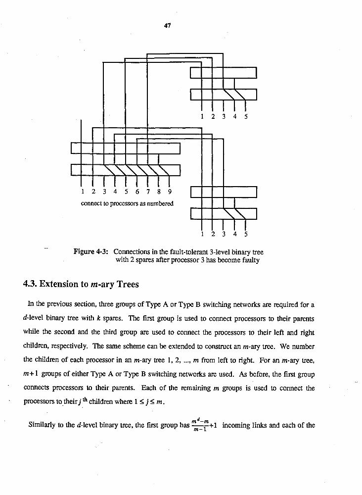
connect to processors as numbered #+ -
Figure 4-3: Connections in the fault-tolerant 3-level binary tree with 2 spares after processor 3 has become faulty
4.3. Extension to m-ary Trees
In the previous section, three groups of Type A or Type B switching networks are required for a
d-level binary tree with k spares. The first group is used to connect processors to their parents
while the second and the third group are used to connect the processors to their left and right
children, respectively. The same scheme can be extended to construct an m-ary tree. We number
the children of each processor in an m-ary tree 1, 2, ..., m from left to right. For an m-ary tree,
m+ 1 groups of either Type A or Type B switching networks are used. As before, the first group
connects processors to their parents. Each of the remaining m groups is used to connect the
processors to.their j th children where 1 5 j I m .
m d-m Similarly to the d-level binary ~ e e , the first group has +1 incoming links and each of the
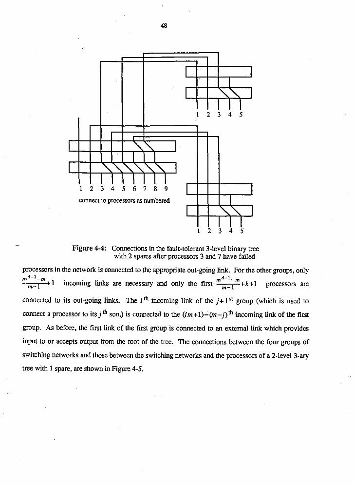
-- Figure 4-4: Connections in the fault-tolerant 3-level binary tree
with 2 spares after processors 3 and 7 have failed
processors in the network is connected to the appropriate out-going link. For the other groups, only rnd-1-m md-1-m
m- 1 +1 incoming links are necessary and only the first m-l +k+l processors are
connected to its out-going links. The i th incoming link of the j+ 1 St group (which is used to
connect a processor to its j th son,) is connected to the (im+l)-(m-j)fi incoming link of the first
group. As before, the first link of the first group is connected to an external link which provides
input to or accepts output from the root of the tree. The connections between the four groups of
switching networks and those between the switching networks and the processors of a 2-level 3-ary
tree with 1 spare, are shown in Figure 4-5.

connect to processors connections to the connections to the connections to the as numbered first son second son third son
Figure 4-5: A fault-tolerant 2-level 3-ary tree with 1 spare
4.4. Comparison with Previous Schemes
The fault-tolerant d-level binary tree constructed using our scheme contains 2d-1 active
processors and k spares. In our reliability analysis, we consider only processor failure. Other types
of failures may be accounted for by the coverage factor [17]. If reconfiguration fails due to these
failures, the entire system is considered to be unreconfigurable.
Let c be the coverage factor, k be the number of spares, d be the level of the binary tree, n = id- 1,
and r be the reliability of a single pmcessor. We define the reliability R4 of our fault-tolerant
d-level binary tree scheme with k spares to be the probability that the particular d-level binary tree
structure remains intact. The reliability RdV0 of a d level non-redundant binary tree is equal to rn
since the failure of any single processor destroys the binary tree structure. For arbitrary k, the
reliability R4 can be obtained using the same procedure as described in Section 2.3.
The comparison of our scheme with the previously proposed scheme is done assuming that the
reliability of a single processor is r=e-k where h is the failure rate of a processor over time t.
Given that r=e-k, the reliability of an d-level binary tree using our scheme with k spare processors
is

In Figures 4-6 and 4-7, the system reliabilities of an 8-level full binary tree using Singh's scheme,
Howells and Agarwal's scheme, Lowrie and Fuchs's SOFT scheme and our scheme are plotted for
h= 0.1 with c= 1 and c = 0.95, respectively. The number of spares used by each scheme is slightly
different. For Lowrie and Fuchs's scheme, 64 spares (the maximum allowable) are used. Since the
only accurate reliability equation given in their paper is for a 4-level tree, the reliability values used
in the figures are approximate and have been obtained by averaging the upper and lower bounds
that they give for their scheme. The lower bound, given in their paper, is the reliability of a
modular tree where each module has three active processors and one spare. The upper bound is the
reliability of a modular tree where each module has three active processors and two spares. This
upper bound (suggested by Howells and Agarwal[9]), is justified because at most two failures can
be tolerated for a node and its two children. With Singh's scheme, 127 spares are used which gives
one spare to each module. This number is the smallest possible number of spares for his scheme
and is already twice as many spares as used by Lowrie and Fuchs's scheme. For Howells and
Aganval's scheme, 48 spares are used. The entire 8-level binary tree is split into a 4-level subtree
containing the root and sixteen 4-level non-root subtrees. The subtree containing the root is
assumed to be implemented using Lowrie and Fuchs's SOFT approach with the spares provided by
the non-root subtrees. The 48 spares are divided equally among the sixteen subtrees so that three
spares are allocated to each non-root subtree. With this number of spares, Howells and Agarwal's
scheme is more reliable than the other two schemes. With our scheme, 25 spares are sufficient to
achieve a higher reliability than the other schemes.
For the range of t shown in Figures 4-6 and 4-7, our curves always lie above the curves of the
other schemes even though our scheme uses fewer spares. At various points in the range 1 < t I 2
there are crossover points where the reliability of the new scheme drops below that of the other
schemes. This must occur eventually since the other schemes use many more spares than our
scheme. However, our scheme can achieve a higher level of reliability than the other schemes
using only a fraction of the spares that are used when t l 1. Intuitively, our scheme is more
reliable since it treats the entire binary tree as a single fault-tolerant module, that is a system with
only k spares can tolerate any k faults in the binary tree. Thus, it is more flexible in its use of
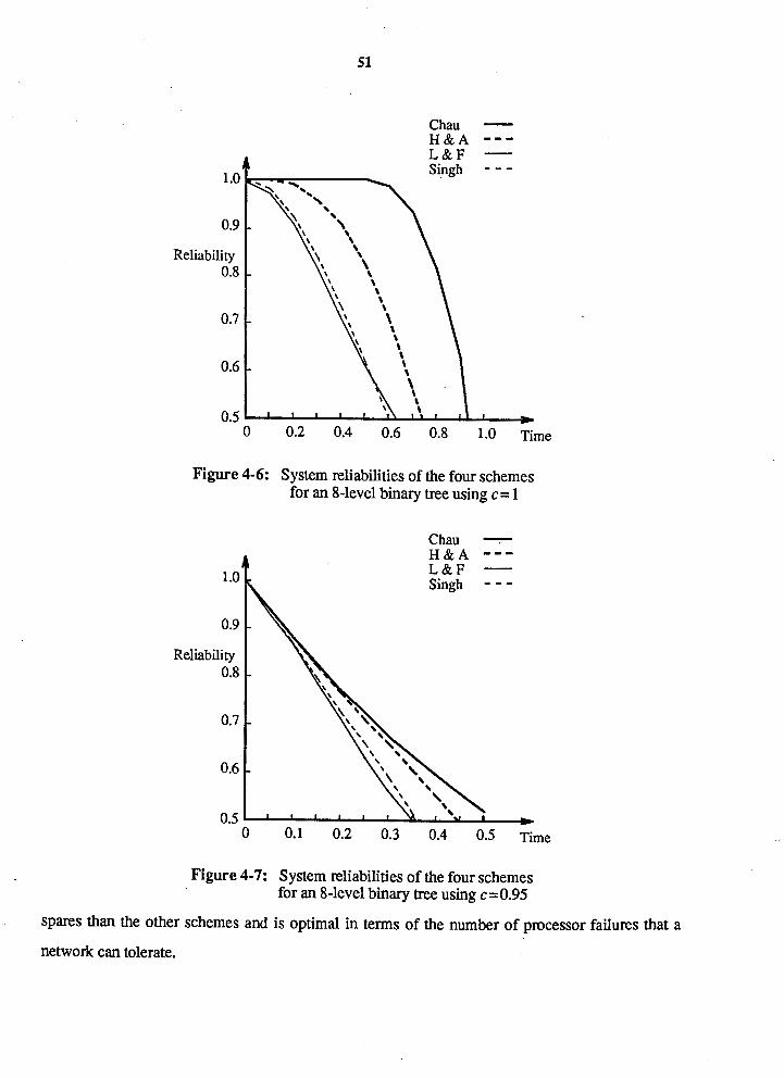
Chau - H & A ---
Figure 4-6: System ~liabilities of the four schemes for an 8-level binary tree using c = 1
Reliability 0.8
Chau - H & A --- L&F - Simgh - - -
Figure 4-7: System reliabilities of the four schemes for an 8-level binary tree using c= 0.95
spares than the other schemes and is optimal in terms of the number of processor failures that a
network can tolerate.

We have also calculated the reliabilities obtained by our scheme and by Mowells and Agarwal's
scheme for an 8-level binary tree with ~ ~ 0 . 9 5 and c = l when both schemes use 48 spares
(approximately 20% of the number of active processors). In this comparison, our scheme achieves
a higher reliability over the range 0 < t 5 2.5. The same result is obtained when we compare our
scheme and that of Lowrie and Fuchs's (with 64 spares each) and when comparing our scheme
with Singh's (with 127 spares each).
The hardware requirements of the different schemes are discussed in terms of two measurements - the number of spares and the number of switches. A clear comparison can be made with the
number of spares required since the hardware required for a spare processor is the same for all the
schemes. The complexity of the switches used by various schemes differs considerably and, thus,
simply counting them is not sufficient. For example, the switches used in our scheme are simpler
than those used in either Lowrie and Fuchs's scheme or in Howells and Agarwal's scheme.
In order to construct a d-level fault-tolerant binary tree, three groups of switching networks are
required. The first one has 2d- 1 incoming links and 2d+ k- 1 outgoing l i i . The other two have
2d- ' - 1 incoming links and 2d- l + k- 1 outgoing links. From the calculations given in Section
2.4, a Type A switching network has (2 n+ k- 1) kj2 switches. If Type A switches are used, the
total number of switches required is k(2(2d- - 1)+ k-1)+ k/2 (2 (2d- 1) + k-1)+2 (2d+ k-2)
= k(2df 2+3 k-9) +2 (2d+ k-2), where 2 (2d+ k-2) is the number of soft switches required to
connect consecutive processors together. Let l= rlog2(k+ 111 and k=$;k iai l i , where the ai 's
are either 0 or 1. From the calculations given in Section 2.5, a Type B switching network has
( n l + ~ ? - ' r = l iai2j) switches. If Type B switching networks are used, the total number of switches
required for our scheme is 2 ~ ( 2 ~ - - 1) + 1(2d- I)+ 3 ~f:: i~~2 '+2(2~-2) . Since a Type B
switching network uses a lot less switches than a Type A switching network, the comparisons given
below assume that Type B switching networks are used.
In Table 4-1, the number of spares and switches required for our scheme to obtain approximately
the same level of reliability as Lowrie and Fuchs's scheme is shown for 4 I d l 12, with t=0.2
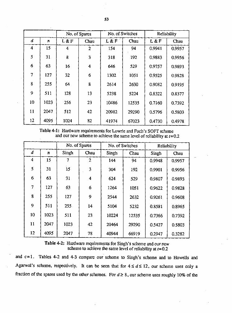
Reliability No. of Spares No. of Switches
Chau
94
192
529
1051
2630
5224
12535
29290
67023
Chau Chau
Table 4-1: Hardware requirements for Lowrie and Fuch's SOFT scheme and our new scheme to achieve the same level of reliability at r=0.2
No. of Spares ( No. of Switches Reliability
Singh
3 304
4 624
6 1264
9 2544
14 5 104
23 10224
42 20464
78 40944
Chau
94
192
529
1051
2632
5232
12535
29290
66919
Chau
0.9957
0.9956
0.9893
0.9828
0.9608
0.8965
0.7392
0.5803
0.3282
Singh Singh
Table 4-2: Hardware requirements for Singh's scheme and our new scheme to achieve the same level of reliability at r=0.2
and c = l . Tables 4-2 and 4-3 compare our scheme to Singh's scheme and to Howells and
Agarwal's scheme, respectively. It can be seen that for 4 1 d 1 12, our scheme uses only a
fraction of the spares used by the other schemes. For d 2 8, our scheme uses roughly 10% of the

spares required by the other schemes and this percentage decreases as d increases. For smaller
values of d, the percentage is somewhat higher but the improvement is still significant. Ford I 10,
the number of switches required is roughly the same as the other schemes. The number of switches
does increase more rapidly for our scheme than Lowrie and Fuch's scheme, and Singh's scheme
when d 2 10. However, the savings in the number of spares when d 2 10 should offset this
increase. For Howells and Agarwal's scheme, the number of switches increases even more rapidly
than our scheme for d 2 10. Thus, the hardware requirement for our scheme is no more than for
the other proposed schemes for 4 I d I 12.
No. of Spares
Chau
No. of Switches
Chau
Reliability
Chau
0.9957
0.9956
0.9580
0.8803
. - 0.9926
0.9800
0.9920
0.98 18
0.9767
TabIe 4-3: Hardware requirements for Howell and Agarwal's scheme and our new scheme to achieve the same level of reliability at t=0.2
Table 4-4 lists the number of spares required for our scheme to achieve a reliability of at least
0.98 at time t=0.4 for 4 I d I 11. It also lists the same values for Howells and Agarwal's scheme
to achieve a reliability of at least 0.98. If a reliability of 0.98 is not achievable, the reliability of
having 100% spares for the sub-trees are listed. The values in Table 4-1, Table 4-2, and Table 4-4
show that our scheme can achieve higher reliability for a longer period of time when d is large.
Thus, it is more suitable for long-life unmaintained systems than the other proposed schemes for
binary trees with a large d.

No. of Spares
Chau
No. of Switches
Chau Chau
Table 4-4: Hardware requirements for Howell and Agarwal's scheme and our new scheme to achieve a reliability of at least 0.98 at t=0.4
4.5. Modular Sparing
It may not be possible to implement an entire binary tree on a single chip. We could use Howells
and Agarwal's scheme to split the binary tree into subtrees with one subtree containing the root.
Each subtree could then be placed on its own chip. The global sparing scheme described in Section
4.2 can be applied to each of the subtrees with additional switching networks used to connect the
leaf nodes of the mot's subtree to the roots of the other subtrees. When a spare processor is used to
replace a failed active processor in the root's subtree, the leaf nodes of the root's subtree will still
be connected to the appropriate roots of the rest of the subtrees.
The connection between the leaf nodes of the root's subtree and the roots of the rest of the
subtrees can be constructed using two groups of switching networks. Let f be the number of leaf
nodes in the root's subtree and k be the number of spare processor in the root's subtree. Both
groups have f incoming links and f+k outgoing l i i . For the first group, the f incoming links are
connected to the left children of the leaf node of the root's subtree. For the second group, the f
incoming links are connected to the right children. The outgoing links of both groups are
connected to the leaf nodes and the spare processors of the root's subtree. The reconfiguration for
this scheme is the same as described in Chapter 2.

Let p=rd/21 level and q=L-j/2J. Assume that we split up a d-level binary tree into a mot's
subtree of one p level and 2P q level subtrees. Each subtree has k spare processors. Using the
same procedure as described in Section 2.3, the reliability of a fault-tolerant binary tree constructed
using the modular scheme is
The number of switches required for this scheme is the sum of the number of switches required to
implement a p level biiary tree, the number of switches required to implement 2P q level binary
trees, and the number of switches required to implement two switching networks with f incoming
links and f+ k outgoing links. The total number of switches required is 2 /(V-l- 1) + l(2P- 1)
3 r = 1 2 +2(2p+k-2) +~(21(2 '7-~-1) +1(2q-1) +3~:1f.=: iai2' +2(2q+k-2))
No. of Spares
Modular Global
Extra Hardware
Modular
8 .O
16.1
24.1
48.2
64.6
161.1
193.8
45 1.6
Global
Reliability
Modular Global
Table 4-5: The amount of extra hardware required to achieve the same level of reliability for the modular and for the global scheme at t=0.4
In Table 4-5, the amount of extra hardware required to achieve the same level of reliability using
modular sparing by splitting an d level biiary tree into one p level subtree containing the root and
2P q level subtrees and using global sparing is shown. The amount of hardware is given in
"processor equivalents", that is the total number of gates divided by 20,000. Each switch is

assumed to be implemented with 10 gates. The values given in Table 4-5 show that global sparing
can achieve the same level of reliability as modular sparing with less hardware. Thus, if possible,
global sparing should be used instead of modular sparing. Furthermore, the values also show that
the extra hardware required to implement the switching network is small compared with the
hardware required to implement the active processors.

Chapter 5 '
Cube-Connected-Cycles Architecture
5.1. Introduction
- As described in Section 1.2.3, a cube-connected cycles (CCC) network consist of n=h2d
processors with h 2 d. In this chapter, a fault-tolerant CCC architecture is proposed. The proposed
scheme uses fault-tolerant modules as building blocks to realize a CCC. In our construction, we
add spare processors to each cycle of the CCC so that each cycle is a fault-tolerant module. A
module with k spares can tolerate up to k faults. Using the same number of spares, the new scheme
is more reliable than Banerjee's schemes [2]. The new modular scheme can also be extended to a
global sparing scheme where the entire CCC can be regarded as a single fault-tolerant module.
That is, the k spare processors in the network can be used to replace any of the active processors in
the ~etwcrk. Wit! global sparing, it is possibie to achieve the same level of reliability as modular
sparing while using significantly fewer spares. In Section 5.2, we propose the new modular
scheme for CCC which is extended in Section 5.5 such that the entire cube-connected-cycles can be
regard as a single fault-tolerant module. In Section 5.3, we present the reliability estimate of the
new modular scheme. In Section 5.4, we compare the reliability of the new modular scheme with
other proposed schemes. In Section 5.6, we compare the reliability and hardware costs of the new
global sparing scheme with those of the new modular sparing scheme.
5.2. New Fault-Tolerant Scheme for Cube-Connected-Cycles
A fault-tolerant CCC can be constructed by connecting fault-tolerant cycle modules together. For
a CCC of 2d cycles where each cycle has h processors, the fault-tolerant CCC consists of 2d
fault-tolerant cycle modules. Each fault-tolerant cycle module has h active processors and k spares,
where k 2 1 .

The h active processors and k spares of a module are connected together to form a cycle. Since
only h processors are active at any given time, spare processors and faulty ones are bypassed using
soft switches in the cycle as shown in Figure 5-1. These fault-tolerant cycles are connected
together to form a fault-tolerant CCC.
The connections between the fault-tolerant cycle modules are realized by using either a Type A or
a Type B switching network such that only active processors in the cycle are connected to other
cycles. The reconfiguration process is as described in Chapter 2. In addition, the faulty processor
must also be disconnected through the use of soft switches from the cycle while the spare processor
immediately to the right of the rightmost active processor becomes an active processor and is
connected to the cycle.
soft' switches
Figure 5-1: A fault-tolerant cycle with k spares
5.3. Reliability Estimate of the Scheme
The fault-tolerant CCC constructed using our modular sparing scheme is a fault-tolerant system
consisting of a series of homogeneous subsystems. Each subsystem is a fault-tolerant cycle with h
active processors and k spare ones. In our reliability analysis, we consider only processor failure.
Other types of failures are accounted for by the coverage factor [17]. If reconfiguration fails due to
the above failures, the entire system is considered to be unreconfigurable. We first give a
reliability analysis of a fault-tolerant cycle.
Let c be the coverage factor, k be the number of spares per cycle, h be the number of active

processor in a cycle, and r be the reliability of a single processor. In each fault-tolerant cycle, at
least h processors must be working. The reliability of a non-redundant cycle RCo is equal to rh.
Using the same procedure as described in Chapter 2, for arbitrary k, h+k-1 h R C ~ = R C ~ - ~ + ( k ) r ( ~ - r ) ~ c ~ .
If the failure rate of a processor is a constant h, the reliability of a single processor is r=e-k.
The reliability of a single module for arbitrary k is h+k-1 R C ~ = R C ~ - ~ + ( ) (e-9h(l-e-qkck.
Finally, the reliability estimate RSd h,k of a CCC with 2d cycles, h active processors and k spare
ones in each cycle, is the product of the reliabilities of a l l the fault-tolerant cycles.
RSd, h, = (R~k)2d-
5.4. Comparison with Previous Schemes
The reliability of a system depends on the number of redundant processors being added.
Although system reliability is not directly proportional to the number of spare processors, the
amount of extra hardware does affect the reliability of a system. If the coverage factor is very close
to one, a higher number of spare processors implies higher reliability. Therefore, we will only
compare reliabiity for systems that use the same number of spare processors. We will compare the
system reliability of our scheme with Banejee's basic and modular schemes. The equation to
calculate the reliability of Banerjee's basic scheme [2] is
d h 2 ' ~ h (!)rh-i(l-r)ici. Rk,=trh)' +2 ( r ) i=1
Let g be the number of processors in a module for Banejee's modular scheme and assume that
h=ig where i and g are integers. The reliability of a fault-tolerant cycle using Banerjee's modular
. scheme [2] is
Rcycle= (rg+grg(l-r)c)i.
The reliability of the entire network is
Rvs = ( ~ ~ ~ ~ l ~ ) ~

Using h=0.1, c= 1 and k= 1, Figure 5-2 shows the system reliability of Rane jee's basic scheme
and our scheme for fault-tolerant CCC with d= 3 and h= 8, and d= 5 and h= 32.
New scheme '
d = 3 Banerjee's basic scheme - - - - - - New scheme
Reliability
0.04 0.08 0.12 0.16 0.20 Time
Figure 5-2: Comparing system reliability of Banerjee's basic scheme and our scheme with d= 3 and h= 8, and d=5 and h= 32
Similarly, using h=0.1, c = l , k=2 and g=h/2, Figure 5-3 shows the system reliability of
Bane jee's modular scheme and our scheme for fault-tolerant CCC with d=5 and h=6, and d= 6
and h= 8. Figures 5-2 and 5-3 show that our scheme has higher reliability than Bane jee's scheme
when the same number of spares are used.
Each fault-tolerant cycle requires only one switching network and there are 2d fault-tolerant
cycles. Thus, the entire network has 2d switching networks, Assuming that Type A switching
networks are used, the total number of switches required is 2d-1 (2h+ k- 1) k. A switch can be
implemented with approximately ten gates. For a cube-connected cycle with h=4 and d=3 which
has 32 active processors, with 2 spare processors in each fault-tolerant cycle, that is 16 spares for

New scheme d = 5 Banerjee's modular scheme - - - - - -
New scheme
t Banerjee's modular scheme - - - - - -
Reliability 0.8
Figure 5-3: Comparing system reliability of Bane rjee's modular scheme using g=h/2 and our scheme withd=5 and h = 6 , and d=6 and h=8
the entire system, the additional hardware required will be approximately 360 gates. If Type B
switching networks are used instead of Type A switching networks, the total number of switches
used will be even less. A single processor can be implemented with roughly 20,000 gates. The
amount of extra hardware required is minimal for our scheme.
5.5. Global Sparing for Cube-Connected Cycles
The new fault-tolerance scheme described in Section 5.2 requires that each fault-tolerant module
must be a cycle. With minor modifications to the scheme, the entire CCC can be a fault-tolerant
module. That is, we can have global sparing where the k spares in the network can back up any k
faults.
In Section 5.2, each module must be a cycle. The fault-tolerant cycles are connected together
through the use of switching networks. The same interconnection technique used to connect fault-

tolerant cycles together can be applied to connect processors together to form a cycle. The
connection of processors into cycles can be realized by at most three groups of switching networks.
For example, for a cycle with four processors, two switching ,networks are sufficient to connect the
processors in a cycle as shown in Figure 5-4. This is done by connecting the lSt and 2nd, and the
31d and 4" incoming communication links of the first switching network. The second group is
used to connect the 2nd incoming communication link to the 31d and connecting the lSt to the 4fh.
Using the two switching networks, processors 1,
extended to cycles with any number of processors.
2, 3 and 4 form a cycle. This scheme can be
connections to the processors as indicated by the number
Figure 5-4: Using 2 Type A switching networb to connect 4 processors together to form a cycle
We now describe how to connect any number of processors together to form cycles. For even h,
two groups of either Type A or Type B switching networks are required. We number the incoming
links to the switching network from 1 to h2d. For the first group, the i incoming link is
connected to the i+ 1 St incoming link if i is odd. For the second group, the i St incoming link is
connected to the i+ 1 St incoming link if i is even and i f 0 mod h. If i = 0 mod h then it is
connected to the (i-h+ 1) St link.
For odd h, three groups of either Type A or Type B switching networks are required. For the first
group, the i " incoming link is connected to the i+ 1 St incoming link if i mod h is odd. For the
second group, the i rh incoming link is connected to the i+ 1 st incoming link if i mod h is even and
is not equal to zero. For the third group, the i h incoming link is connected to the i+h-lst
incoming link if i 5 1 mod h . These connections will connect the processors into 2d cycles with h

processors in each cycle. For example, in Figure 5-5, processors 1 to 5 and processors 6 to 10 are
connected as cycles through the three switching networks.
- - - - ' first group
. . b . . \ . . . \ \ \ \ \ \ \ \ \ \ \ \ \ \ \ \ \ \ \ \ I
I
- - - - second group
connect to processors as numbered
Figure 5-5: Connecting 10 processors into 2 cycles with 5 processors each using 3 switching networks
After the processors are connected to form cycles, one more switching network is required to
connect all the cycles together to form a CCC. Let i = j mod h . For this switching network, the i th
incoming link, if it is not already connected to another incoming link, is connected to the (2j-l h)
incoming link where 1 I j I d . In addition to the switching networks, consecutive processors are
connected together as in Chapter 2 to provide fast context switching and distributed
- reconfiguration. Finally, the reconfiguration for this global sparing scheme is exactly the same as
. the one using a cycle as a fault-tolerant module.
A CCC with d=2, h=4 and 1 spare for the entire network is shown in Figure 5-6. Three Type A
or Type B switching networks afe required. The first two are used to create the connection for the
four cycles and the third is used to connect the cycles together to form the fault-tolerant CCC.

connect to processors as numbered
Figure 5-6: A fault-tolerant CCC with d= 2, h =4 and 1 spare for the entire network
5.6. Comparing Global Sparing with other Proposed Schemes
Let c be the coverage factor, k be the number of spares for the entire CCC, and r be the reliability
of a single processor. Using the same procedure as described in Section 2.3, the reliability RGk of
a fault-tolerant CCC with 2d cycles each has h active processors and k spare processors using
global sparing is
h2d+k-l h2d R G ~ = R G ~ - ~ + ( k ) r (I-rlkck.
Although any fixed reliability, say 0.999, may not be achievable due to the coverage factor c [17],
global sparing achieves the highest reliability possible. In Table 5-1, the number of spares required
for global sparing to obtain the same level of reliability as Banerjee's modular scheme with t=0.1
and c = l , is given for 2 < d l 8, g=2 and h=d if d is even or h=d+l if d is odd. From the

values given in Table 5-1, it is clear that global sparing can achieve the same level of reliability as
Banerjee's modular scheme or our modular scheme using only a fraction of the spares used by
those schemes.
No. of Spares Reliability
Bane rjee
8
16
32
64
128
256
512
Global B anerjee Global
Table 5-1: The number of spares required to achieve the same level of system reliability for Banerjee's modular sparing scheme and the
global sparing scheme using h= 0.1 , t= 0.1 , c = 1 and h=d if d is even or h=d+ 1 if d is odd
,.-
Fcr even d, thze g m p s ~f switchiiig neiw~ikS are required to construct the fault-tolerant cube-
connected-cycles. For odd d, four group are required. Let 1 = log2 k+ 1 and k = ~ i l i ai2', where
the ai9s are either 0 or 1. From Section 2.5, each Type B switching network has n l + ~ f . i : iai2'
switches. Hence, if Type B switching networks are used for the construction and d is even, the
total number of switches required is 3 (2dhl+%;: iai2i)+2(2dh+ k- 1). If d is odd, the total
number of switches required is 4 ( 2 d h l + ~ i ~ : iai2i)+2(2dh+ k- 1).
We assume that a processor can be implemented with 20,000 gates [17] and a switch can be
implemented with 10 gates. In Table 5-2, the number of spares and the amount of extra hardware
required for global sparing to obtain the same level of reliability as the modular scheme using a
cycle as a fault-tolerant module with t = 0.1 and c = 1 is given for 2 I d I 8, h = d and 2 spares per
module. The amount of extra hardware is given in "processor equivalents", that is, the total
number of gates divided by 20,000. The values in Table 5-2 shows that the amount of hardware
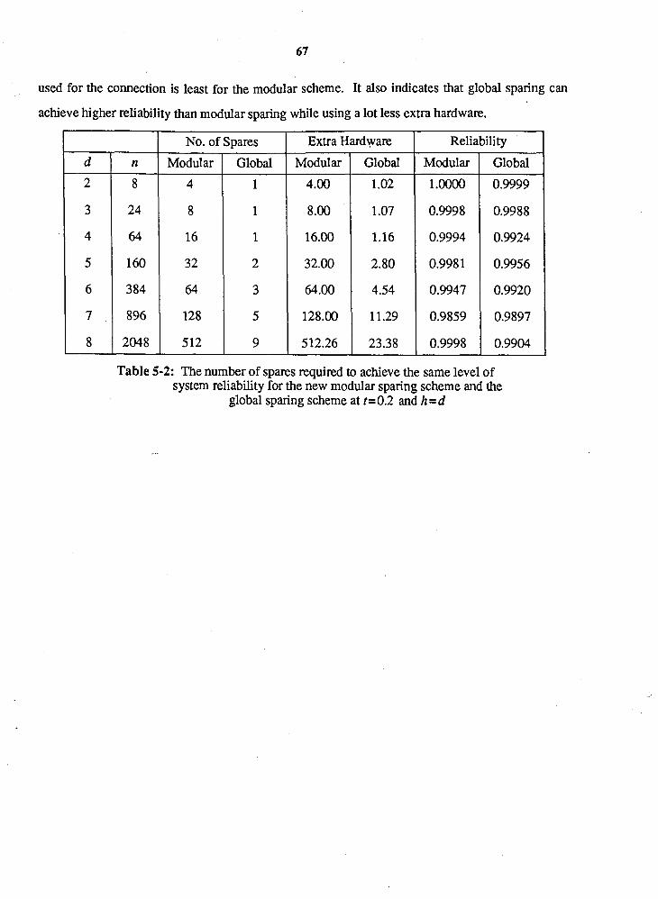
67
used for the connection is least for the modular scheme. It also indicates that global sparing can
achieve higher reliability than modular sparing while using a lot less extra hardware. - --
No. of Spares
Modular Global
Extra Hardware
Modular Global
Reliability
Modular Global
Table 5-2: The number of spares required to achieve the same level of system reliability for the new modular sparing scheme and the
global sparing scheme at t=0.2 and h =d

Chapter 6
Multistage Interconnection Networks
6.1. Introduction
As described in Section 1.2.4, a multistage interconnection network (MIN) architecture can be
characterized as having n=2m processors connected together by m stages of switching elements.
In this chapter, a new fault-tolerant multistage interconnection network architecture that can
tolerate processor failures as well as connection failures is proposed. The proposed scheme can
provide coverage either for processor failures or for both processor and connection failures.
Furthermore, other previously proposed schemes could be used to provide coverage for connection
failures while the new scheme is used to provide coverage for processor failures. Our new scheme
can be used to incorporate k spare processors in the network which can tolerate any k processor
failures. In comast, Jeng a ~ d Siegel's OR scheme c a ~ only tolerate a single processor failure or
very limited instances of multiple failures for the entire network (or for a given module) if more
than one spare processor is used.
In Section 6.2 a new fault-tolerant scheme for multistage interconnection network architecture is
proposed which uses the switching networks described in Chapter 2. In Section 6.3, we compare
the reliability of our scheme with that of Jeng and Siegel's DR scheme. The scheme is extended in
Section 6.4 to cover both processor failures and switching element failures. In Section 6.5, the
extended scheme is compared to Jeng and Siegel's DR scheme. Finally, the hardware requirements
for variants of our scheme are discussed in Section 6.6.

6.2. New Fault-Tolerant Scheme For Multistage Interconnection Networks
In this section we propose a new scheme that provides coverage for processor failures. A
multistage interconnection network or a fault-tolerant multistage interconnection network that can
tolerate switching element failures and link failures, can be realized by different kinds of
interconnections [I]. The new scheme can be applied to almost all of the previously proposed
non-fault-tolerant or fault-tolerant interconnection schemes.
A multistage interconnection network can be characterized as having n=2m processors connected
together by log2n stages of switching elements as shown in Figure 6-1. If we only consider
processor failures, a fault-tolerant MIN functions properly when its input and output links are all
connected to non-faulty processors. When a processor fails, if we can disconnect it from the input
and output links of the h4IN and reconnect the links to a new non-faulty processor, the MIN will
function properly. This can be done by inserting either Type A or Type B switching networks
between the processors and the m stages of switching elements as shown in Figure 6-2.
connections to the processors as numbered
- - - n m
Figure 6-1: A multistage interconnection network
We construct a k fault-tolerant MIN with n active processors and k spare processors using two
groups of either Type A or Type B switching networks. One group is used to connect the input
links of the stages of switching elements to the processors while the other group connects the
output links of the stages of switching elements to the processors. These two switching networks
log n stages of switching elements
-
- - C
n

log n stages of
switching elements
switching networks
C
* - - - - - -
- T *
connections to the links processors as numbered
Figure 6-2: A fault-tolerant multistage interconnection network
are used to replace faulty processors with spare ones if required. We number the processors from 1
to n+ k such that processor i is connected to processor i-1 , where 1 c i I n+ k. Soft switches are
used to bypass faulty processors as described in Section 2.6. When a processor fails, the
reconfiguring process described in Chapter 2 is initiated. With our scheme, no extra control
information is needed for the fault-tolerant MIN to function properly. The fault-tolerant MIN can
operate as if it is a non-redundant MIN and no modification to the routing is required. Hence, our
scheme is more adaptable than other schemes such as the DR network which requires additional
routing tags to be added.
6.3. Reliability Estimation of the Scheme
The fault-tolerant MIN constructed using our scheme contains n active processors and k spares.
In analyzing its reliability, we consider only processor failure. The failure of switching elements
can be covered by other proposed methods [I]. Let c be the coverage factor, k be the number of
spares processors in the MIN, n be the number of active processors in the MIN, s be the reliability
of a single switching element, w be the reliability of a row of switches used in the DR network,
sO=snI2 be the reliability of a stage of switching elements in a MIN with no spare switching
element, r be the reliability of a single processor and m= log2n. The reliability of a non-redundant
MIN Ro is rns;.

Using the same calculations as in Section 2.3, for arbitrary k,
m n+k-1 Rk= Rk-l+So ( k ) rn( l -r )kck.
Jeng and Siege1 [ lo] showed that the optimal number of spares in a DR network is one in that no
further improvement in reliability can be achieved with more spares. However, with our scheme,
the optimal number of spares depends on the value c and is much larger than one. Thus, our
scheme can achieve higher reliability than Jeng and Siegel's scheme by using multiple spares. In
fact, our scheme with only two spares provides higher reliability than Jeng and Siegel's DR
network when n 2 200 and r=0.99 even though our scheme only provides coverage for processor
failures.
Lemma 1: Assuming that w 2 r and c= 1 , our scheme with two spares has a higher
reliability than the DR network with one spare processor and one extra row of switching 2f
elements when n > =- 1 .
Proof: As shown in [ lo] , the reliability of the DR network with one spare is
(rw)"+(n+ l)(rw)"(l-rw).
The reliability of our scheme w i a t w s p m s is
We now show that (2) > (1).
Since $ = (sf l )* 2 w ", we can divide ( 1 ) by (rw)" and (2) by rns;.
Since w 2 r , ( 1 -r) 2 ( 1 -w). Thus, we can divide the RHS by ( 1 -w) and the LHS by
( 1 -r) and simplify both sides further. LHS=(n+ 1)(1-r)/2. RHS=r.
Putting n on the LHS. LHS=n.

Thus, the LHS is greater than the RHS. 0
According to this lemma, for low values of r (such as 0.9) our scheme using two spares and no
switching element coverage is more reliable than the DR network with one spare processor and one
spare row of switching elements when n 2 18. For higher values of r, the value of n has to be
higher for our scheme to be more reliable than the DR network. For example, when r= 0.99, n
must be greater than 198. However, when directly comparing the computed reliabilities of both
schemes, our scheme with two spare processors actually achieves higher reliability for smaller n
and larger r since some of the cancellations in the proof of the Lemma are biased towards Jeng and
Siegel's scheme.
Let r=e -q t and s=e-%' [17] where kp is the failure rate of a processor over time t and ks is the
failure rate of a switching element over time t [17]. Table 6-1 shows the system reliability of Jeng
and Siegel's scheme with one spare processor and one spare row of switching elements, and the
system reliability of our scheme with two spare processors with $=O.l and h,=0.01. According
to these figures, our scheme is better for r S 0.99 when n 2 32 and for r in the range
0.99 I r I 0.999, our scheme is better for n 2 512. Our scheme can achieve even higher system
reliability with more than two spare processors and by adding other proposed schemes to cover
switching element failures. Thus, our scheme should be able to achieve higher reliability than the
DR networks for smaller n and larger r.
6.4. Extension to Cover Switching Element Failures
In Section 6.2, switching networks are used to provide coverage for processor failures. The same
technique can also be applied' to provide coverage for switching element failures on a variety of
MINs such as the generalized cube, the omega network, the shuffle exchange network and the
baseline network. In this section, we show how the technique can be applied to cover switching
element failures in shuffle exchange networks. Figure 6-3 shows a shuffle exchange network with
eight processors. A shuffle exchange network has the nice property that the connections between

System Reliability
Chau Chau
0.9996
0.9988
0.9968
0.9920
0.9809
0.9559
0.9006
0.7820
0.5484
0.2151
0.0192
Chau
Table 6-1: The system reliability of Jeng and Siegel's DR scheme and our new scheme with k=2
any two stages of the switching elements are exactly the same. Hence, we only have to show how
the technique can be used between any two stages. Figure 6-4 shows the connection between two
stages of switching elements in a shuffle exchange network with 8 active processors and one spare
switching element in each stage.
Fault-tolerance in the switching elements can be provided by inserting four groups of switching
networks between two stages of switching elements. In this case, the switching networks serve to
collect the outputs from the active switching elements in stage i and direct them to the active
switching elements in stage i+ 1. Collecting the outputs from the active switching elements in
stage i is done by the first and second group of switching networks, the first one dealing with the
first output of each switching element and the second one dealing with the second output of each
switching element. Similarly, the third and fourth groups of switching networks are used to direct
these outputs to the inputs of the active switching elements of stage i+ 1 - the third group for the

switching elements
stage 0 stage 1 stage 2
Figure 6-3: A shuffle exchange network with 8 processors
connections to switching elements in stage i
1 2 3 4 5 1 2 3 4 5
1 2 3 4 5 1 2 3 4 5
connections to switching elements in stage i+l
second group
fourth group
Figure 6-4: The connection between 4 groups of switching networks
first inputs and the fourth group for the second inputs of the switching elements. The standard
shuffle exchange interconnection is used to connect these four groups of switching networks. In
general, for a shuffle exchange network with n processors, the i fh output link of the first group of

switching network is connected to the (2i- input link of the third group if 2i I n/2. Otherwise,
it is connected to the (2i- 1 -n/2)h input link of the fourth group. Similarly, the i th output link of
the second group is connected to the 2i th input link of the third group if 2i 5 n/2. Otherwise, it is
connected to the (2i-n12)~ input link of the fourth group.
Between the processors and the switching elements, two additional groups of switching networks
are required to provide coverage for stage 0 and the last stage. The first group connects the first
input or output links of the switching elements to the processors depending on whether it is the first
or the last stage and the second group connects the second input or output links. The connections
between the processors and the two groups of switching networks are similar to the connections
between the four groups of switching networks for any two stages. The i th link of the first group is
connected to the (2i- processor and the i th link of the second group is connected to the 2i th
processor. With these switching networks and f spare switching elements in each stage, each stage
of switching elements can tolerate up to f switching element failures. Furthermore, the shuffle
exchange MIN can tolerate up to k processor failures using the scheme described in Section 6.2.
This technique can clearly be applied to other types of MIN's besides the shuffleexchange
networks and no additional control information is required by the fault-tolerant MIN.
6.5. Reliability of the Extended Scheme
The fault-tolerant MIN constructed using our extended scheme can tolerate both processor
failures and switching element failures. In our analysis, we do not consider the failures in the
switching networks. However, these failures can be covered by duplicating the switching
networks.
Consider a MIN with n active processors and k spares, n switching elements and f spare switching
elements in each stage of switching elements. Let c be the coverage factor, m= log2n be the
number of stages of switching elements, s be the reliability of a switching element, and r be the
reliability of a single processor. The reliability Po of n processors with no spare is rn . The
reliability So of a stage of non-redundant switching elements is snf2. The reliability Rope of a

non-redundant MIN is P ~ s ~ . Using the the same procedure as described in Section 2.3, the
reliability Rt is given by
Rk = ~ $ 7 where
pk = ck L = O (n+f-l)rn(l-r)ici
and
f ("2tf-1 4 2 1 ici sf=Z,=o , )s - .
Assuming that the switching elements used in the DR network and our scheme have the same
reliability, and Xp=O.l and h,=0.01, the system reliabilities of both schemes with one spare
processor and one switching element per stage are listed in Table 6-2. The values show that our
scheme is at least as good as the DR network when t is small and is better for larger t.
System Reliability
Chau Chau Chau
Table 6-2: The system reliability of Jeng and Siegel's DR scheme and our new scheme with one spare processor and one spare switching element per stage

In general, the amount of extra hardware used in our scheme is k spare processors, f logzn spare
switching elements and 410g2n groups of switching networks. With k=f=l, each group of
switching network has n/2 switches. The total number of extra switches used in our scheme is
2nlog2n. For Jeng and Siegel's DR scheme with k=f= 1, the number of extra links required is
(n+3)log2n. Thus, our scheme uses slightly more extra hardware than Jeng and Siegel's DR
scheme but our scheme can achieve higher reliability using the same number of spare processors
and spare switching elements. Furthermore, with k > 1 and f > 1, our scheme can provide multiple
fault coverage for processors and switching elements. In fact, with k spare processors, our scheme
can tolerate any k processor failures. Similarly, with f spare switching elements in each stage, our
scheme can tolerate any f switching element failures in any stage.
Table 6-3 lists the system reliability of MINs using different values for k and f with hp=O.l and
hs=O.O1 at t=0.01 and t=0.1. The values clearly show that significant improvement can be
achieved by using more than one spare processor and one spare switching element per stage. For a
MIN with 4,096 processors, the reliability at t=0.01 can be improved from 0.08455 for a MIN
with 1 spare processor and 1 spare switching element per stage to 0.99 by using 9 spare processors
and 9 spare switching elemems per stagc.
Table 6-4 shows the number of spare processors and the number of spare switching elements per
stage required to achieve a reliability of at least 0.98 at t=0.01 and t=0.1 for different values of n.
The values in Table 6-4 shows that our scheme can provide high reliability for MDTs with large
numbers of processon and for a longer period of time compared to other proposed schemes by
incorporating more than one spare processor and more than one spare switching element per stage.
The reliability that can be achieved by our scheme is only restricted by the value of the coverage
factor c [17]. Hence, our scheme with multiple spare processors and multiple spare switching
elements is well-suited for use in long-life unmaintained applications.

System Reliability
Table 6-3: The system reliability of our new schezne with different values of k and f
6.6. Modular Sparing
For a MIN with a large number of processors, it may not be feasible to implement an entire MIN
on a single chip. It may be necessary to split up the MIN into smaller modules and connect these
modules together to form the MIN. Our new schemes can be applied to each module.
Let g be the number of modules, rn be the number of active processors in a module, k be the
number of spare processors in each module, Z= rlog2k+ 11, and k = ~ : i : ai2' where the ai 's are
either 0 or 1. The number of switching networks required to provide processor failure coverage
depends on the number of module used. Each module requires 2 switching networks. Hence, 2g
switching networks are required. Since a Type B switching network has a lot less switches than a
Type A switching network, we assume that the fault-tolerant MINs are implemented using Type B
switching networks. From Section 2.5, a Type B switching network has ( n l c ~ ; ~ : - inizi)

Reliability
Chau
1.0000
1.0000
0.9999
0.9995
0.9980
0.9923
0.9977
0.9846
0.9959
0.9815
0.9905
Reliability
Chau
Table 6-4: The number of spare processors, k, and spare switching element, f, per stage required to achieve a reliability of at least 0.98
switches. The total number of switches required to implement a fault-tolerant MIN is
2g(ml+g1: - iai2i)+2g(m+k-l), where 2g(m+k-1) is the number of switches required to
connect consecutive processors together in each module.
Let d= log2n and f be the number of spare switching elements in each module. For the extended
scheme, each module requires 4d switching networks. The total number of switches required to
implement all the switching network is 4 g d ( l m ~ + ~ : ~ : - ioi2{). An additional 2g(m+ k- 1)
switches are required to connect the consecutive switching elements together. The total switches
required for the extended scheme is the sum of the number of switches given above together with
the number required to provide coverage for processor failures. The total number of switches
required for the extended scheme is (4gd+2g)(ml+~:~: - iai2i) + 2g(m+k-1) + 2gd(m+f-1).
For the scheme that provides coverage for processor failures only, the amount of extra hardware

required for modular sparing is always greater than that of global sparing. In Table 6-5, the amount
of extra hardware required to achieve the same level of reliability for global sparing and for
modular sparing with 2 and 4 modules respectively at t=0.01 is shown. The amount of extra
hardware required is given in "processor equivalents", that is the total number of gates divided by
20,000, and each switch is assumed to be implemented with 10 gates. The values clearly shown
that global sparing is better for n I 4096.
No. of Spares Extra Hardware
Global
1
1
1
1
2
3
4
5
7
9
13
Global Global
0.9996
0.9988
0.9967
0.9915
0.9809
0.9562
0.9027
0.7942
0.5993
0.3242
0.0856
Reliability
Table 6-5: Extra hardware required for global sparing and modular sparing with 2, and 4 modules having the same level of reliability at t=0.01 and c= 1
For the extended scheme, the situation is more complicated due to the small size of a switching
element. That is, the savings in the number of spare switching elements for global sparing cannot
offset the extra number of switches required. Table 6-6 and Table 6-7 list the same values as in
Table 6-5 using the extended scheme for t=0.01 and t=0.1, respectively, where a switching
element is assumed to be implemented with 100 gates. The values show that it is better to split the
MIN into more modules as n increases.

No. of Spares
Global
Extra Hardware
Global Global
1 .m 1 .m 0.9999
0.9995
0.9980
0.9923
0.9977
0.9846
0.9959
0.9815
0.9905
Reliability
rable 6-6: Extra hardware required for global sparing and modular sparing using the extended scheme at t=0.01 and c= I

No. of Spares
Global
82
Extra Hardware
Global Global
Reliability
Table 6-7: Extra hardware required for global sparing and modular sparing using the extended scheme at t= 0.1 and c = 1

Chapter 7
Conclusion
Two types of switching networks and a scheme for constructing fault-tolerant multi-computer
networks using these switching networks to interconnect the processors have been proposed. The
scheme can be applied to several types of multi-computer network architectures with only minor
modifications. With our scheme, we can provide global sparing in which the network is
k-fault-tolerant with only k spares. This is clearly optimal in terms of spares required to achieve
k-fault-tolerance. Our global sparing scheme compares favorably with other proposed schemes for
multi-computer networks. It can achieve higher reliability than the other proposed schemes using
no more extra hardware. In most cases, it only uses a fraction of the extra hardware required by the
other schemes to achieve the same level of reliability as the other schemes. Furthermore, the
amount of extra hardware used is small compared to the hardware requirements of a non-redundant
network.
If a network is too large to be implemented as a single fault-tolerant module, a modular approach
can be used using the same technique. In most architectures where the number of switches
required to implement the network is small, global sparing can achieve the same level of reliability
as modular sparing using only a fraction of the extra hardware used for modular sparing. However,
for architectures that require a large number of switches in the connection, the result is not as clear.
In particular, modular sparing may be better when the network has a large number of active
promssors.
A fault-tolerant multi-computer network constructed using our new scheme functions as if it was
a non-redundant network. No extra control information is needed to ensure the fault-tolerant
network bctions properly. When a processor fails, the reconfiguring process can be initiated

distributively. Fast context switching is also provided to speed up reconfiguration. These
properties together with the ability to provide a high level of reliability for a long period of time
make our scheme suitable for long-life unrnaintained applications.

References
G . B. Adams, D. P. Agarwal and H. J. Siegel. A Survey and Cornparsion of Fault-Tolerant Multistage Interconnection Networks. Computer : 14-27, June, 1987.
Prithviraj Banerjee, Sy-Yen Kuo, and W. K. Fuchs. The Cubical Ring Connected Cycles: A Fault-Tolerant Parallel Computation Network. In Digest of papers of the International Symposium on Fault-Tolerant Computing, pages
286-291. The Computer Society, IEEE, 1986.
Prithviraj Banerjee. The Cubical Ring Connected Cycles: A Fault-Tolerant Parallel Computation Network. IEEE Transactions on Computers c-37(5):632-636, May, 1988.
Siu-Cheung Chau and Arthur L. Liestman. A Proposal for a Fault-Tolerant Binary Hypercube. In Digest of papers ofthe International Symposium on Fault-Tolerant Computing, pages
323-330. The Computer Society, IEEE, 1989.
Siu-Cheung Chau and Arthur L. Liestman. A Fault-Tolerant Binary Tree Architecture. Technical Report CMlT TR 88-8, School of Computing Science, Simon Fraser
University,December, 1988.
Siu-Cheung Chau and Arthur L. Liestman. A Fault-Tolerant Multistage Interconnection Network Architecture. Technical Report CMPT TR 89-1, School of Computing Science, Simon Fraser
University,March, 1989.
A. S. M. Hassan and V. K. Agarwal. A Fault-Tolerant Modular Architecture for Binary Trees. IEEE Transactions on Computers c-35(4):356-361, April, 1986.
J. Hastad, T. Leighton and M. Newman. Reconfiguring a Hypercube in the Presence of Faults. Proceedings of Principles of Distributed Computing Conference :274-284,1987.
M. Howells and V. K. Agarwal. A Reconfigurating Scheme for Yield Enhancement of Large Area Binary Tree
Architectures. IEEE Transactions on Computers c-37(4):463-468, April, 1988.
M. Jeng and H. J. Siegel. Design and Analysis of Dynamic Redundancy Networks. IEEE Transactions on Computers c-37(9):1019-1029, September, 1988.

C. L. Kwan and S. Toida. Optimal fault-tolerant realizations of hierarchical tree systems. In Digest ofpapers of the International Symposium on Fault-Tolerant Computing, pages
176-178. The Computer Society, IEEE, 198 1.
Mathew B. Lowrie and W. Kent Fuchs. Reconfigurable Tree Architectures Using Subtree Oriented Fault Tolerance. IEEE Transactions on Computers c-36(10): 1172-1 182, October, 1987.
F. P. Preparata and J. Vuillemin. The Cube-Connected Cycles. A Versatile Network for Parallel Computation. Communications of the ACM :30-39, May, 1981.
C. S. Raghavendra, A. Avizienis and M. D. Ercegovac. Fault Tolerance in Binary Tree Architecture. ZEEE Transactions on Computers c-33(6):568-572, June, 1984.
David A. Remels. On Implementing Fault-Tolerance in Binary Hypercubes. In Digest of papers of the International Symposium on Fault-Tolerant Computing, pages
344-349. The Computer Society, IEEE, 1986.
Adit D. Singh. A Reconfigurable Modular Fault Tolerant Binary Tree Architecture. In Digest of papers of the International Symposium on Fault-Tolerant Computing, pages
298-304. The Computer Society, IEEE, 1987.
D. P. Siewiorek and R. S. Swarz. The Theory and Practice of Reliable System Design. Digital Press, Bedford, MA, 1982.
Raif M, Yanney and John P. Hayes. Distributed Recovery in Fault-Tolerant Multiprocessor Networks. ZEEE Transactions on Computers c-35(10):871-879, October, 1986.
Raif M. Yanney and John P. Hayes. Fault Recovery in Distributed Processing Loop Networks. Computer Networks and ISDN Systems (1 5):229-243,1988.