Fault-Tolerant Programming Models and Computing Frameworks

Candidacy Examination

12/11/2013

Mehmet Can Kurt

2

Increasing need for resilience• Performance is not the sole consideration anymore.

• increasing number of components decreasing MTBF• long-running nature of applications (weeks, months)• MTBF < running time of an application

• Projected failure-rate in exascale era: every 3-26 minutes

• Existing Solutions• Checkpoint/Restart

• size of checkpoints matter (ex: 100000 core job, MTBF=5 years, checkpoint+restart+recomp.=65% of exec.)

• Redundant Execution • low-resource utilization

3

Outline

• DISC: a domain-interaction based programming model with support for heterogeneous execution and low-overhead fault-tolerance

• A Fault-Tolerant Data-Flow Programming Model

• A Fault-Tolerant Environment for Large-Scale Query Processing

• Future Work

4

DISC programming model• Increasing heterogeneity due to several factors;

• decreasing feature sizes• local power optimizations• popularity of accelerators and co-processors

• Existing programming models designed for homogeneous settings

• DISC: a high-level programming model and associated runtime on top of MPI Automatic Partitioning and Communication Low-Overhead Checkpointing for Resilience Heterogeneous Execution Support with Work Redistribution

DISC Abstractions• Domain

• input-space as a multidimensional domain• data-points as domain elements• domain initialization by API• leverages automatic partitioning

• Interaction between Domain Elements• grid-based interactions (inferred from domain type)• radius-based interaction (by cutoff distance)• explicit-list based interaction (by point connectivity)

6

compute-function and computation-space

• compute-function• a set of functions to perform main computations in a program• calculate new values for point attributes

• ex: jacobi and sobel kernels, time-step integration function in MD

• computation-space• any updates must be directly performed on computation-space• contains an entry for each local point in assigned subdomain

7

Work Redistribution for Heterogeneity• shrinking/expanding a subdomain changes processors’

workload

• ti: unit-processing time of subdomain i

ti = Ti / ni

Ti = total time spent on compute-functions

ni = number of local points in subdomain i

8

Work Redistribution for Heterogeneity

1D Case• size of each subdomain should be inversely

proportional to its unit-processing time

2D/3D Case• express as a non-linear optimization problem

min Tmax

s.t. xr1 * yr1 * t1 <= Tmax

xr2 * yr1 * t2 <= Tmax

…

xr1 + xr2 + xr3 = xr

yr1 + yr2 = yr

9

Fault-Tolerance Support: Checkpointing

1. When do we need to initiate a checkpoint? end of an iteration forms a natural point

2. Which data-structures should be checkpointed?computation-space captures the application-state

2D-stencil checkpoint file MD checkpoint file

10

Experiments

• Implemented with C language on MPICH2• Each node with two-quad core 2.53 GHz Intel(R) Xeon(R)

processor with 12GB RAM• Up to 128 nodes (by using a single core at each node)

Applications• Stencil (Jacobi, Sobel)• Unstructured grid (Euler)• Molecular dynamics (MiniMD)

11

Experiments: Checkpointing

Jacobi MiniMD

- Comparison with MPI Implementations (MPICH2-BLCR for checkpointing)

• 4 million atoms for 1000 it.• Checkpoint freq: 100 it.• Checkpoint size: ~2GB vs 192 MB

• 400 million elements for 1000 it.• Checkpoint freq: 250 it.• Checkpoint size: 6 GB vs 3 GB

42%60%

12

Experiments: Heterogeneous Exec.

Sobel MiniMD

- Varying number of nodes slowed down by %40

• Load-balance freq: 200 it. (1000 it.)• Load-balance overhead: 1% • Slowdown: 65% 9-16%

• Load-balance freq: 20 it. (100 it.)• Load-balance overhead: 8% • Slowdown: 64% 25-27%

Experiments: Charm++ Comparison• Euler (6.4 billion elements for 100 iterations)• 4 nodes are slowed down out of 16• Diff. Load-Balancing Strategies for Charm++ (RefineLB)• Load-balance once at the beginning

(a) Homog.: Charm++ 17.8% slower than DISC

(c) Heter. LB: Charm++, at 64-chares (best-case), 14.5% slower than DISC

14

Outline

• DISC: a domain-interaction based programming model with support for heterogeneous execution and low-overhead fault-tolerance

• A Fault-Tolerant Data-Flow Programming Model

• A Fault-Tolerant Environment for Large-Scale Query Processing

• Future Work

Why do we need to revisit data-flow programming?

• Massive parallelism in future systems• synchronous nature of existing models (SPMD, BSP)

• Data-flow programming• data-availability triggers execution• asynchronous execution due to latency hiding

• Majority of FT solutions in the context of MPI

Our Data-Flow Model

Tasks• Unit of computation• Consumes/produces a set of

data-blocks• Side-effect free execution• Task-generation

• via user defined iterator objects• creates a task descriptor from a

given index

Data-Blocks• Single assignment-rule• Interface to access a data-

block; put() and get()• Multiple versions for each

data-block

Task T

(di, vi)

for each version vi (int) size (void*) value (int) usage_counter (int) status (vector) wait_list status=not-ready

(di, vi)

status=readyusage_counter=3status=readyusage_counter=2status=garbage-col.

(di, vi)

status=readyusage_counter=1

(di, vi)

Work-Stealing Scheduler• Working-phase

• enumerate task T• check data-dependencies of T• if satisfied, insert T into <ready queue>

otherwise, insert T into <waiting queue>

• Steal-phase• a node becomes a thief• steals tasks from a random victim• unit of steal is an iterator-slice

• ex: victim iterator object operating on (100-200).

thief can steal the slice of (100-120) leaving (120-200) to victim.

Repeat until no tasks can be executed

Fault-Tolerance Support• Lost state due to a failure includes;

• task execution in failure domain (past, present, future)• data-blocks stored in failure domain

• Checkpoint/Restart as traditional solution• Checkpoint execution-frontier• Roll-back to latest checkpoint and restart from there• Downside: significant task re-execution overhead

• Our Approach • Checkpoint and Selective Recovery

• task recovery• data-block recovery

Task Recovery• Tasks to recover:

• un-enumerated, waiting, ready and currently executing• should be scheduled for execution

• But, work-stealing scheduler implies that• tasks in failure domain are not know a-priori

• Solution:• victim remembers the steal by (stolen iterator-slice, thief id) pair• construct working-phases in failure domain by asking alive nodes

Data-Block Recovery• Identify lost data-blocks and re-execute completed tasks to

produce them

• Do we need (di,vi) for recovery?• not needed if we can show that its status was “garbage-collected”

• consumption_info structure at each worker• holds number of times that a data-block version has been consumed

Uinit=initial usage counter

Uacc=number of consumptions so far

Ur=Uinit – Uacc (reconstructed usagecounter)

Case1: Ur == 0Case2: Ur > 0 && Ur < Uinit

Case3: Ur == Uinit

(not needed)(needed)

(needed)

Data-Block Recovery

T1

T6

T4

T7

T2 T3

T5

d2 d3

d1

d5 d6

d7

d4

T10

T8 T9

T11

Uinit Uacc Ur

d1 1 1 0

d2 1 0 1

d3 1 0 1

d4 1 0 1

d7 2 1 1

completed task

ready task

gc. data-block

ready data-block

We know that T5 won’t be

re-executed Uinit Uacc Ur

d1 1 1 0

d2 1 0 0

d3 1 0 0

d4 1 0 1

d7 2 1 1

* Re-execute T7 and T4

Transitive Re-execution

T1

T3

T4

T2

T5

d4

d1

completed task

ready task

gc. data-block

ready data-blockd2 d3

d5

T6 T7

• produce d1, d5

• re-execute T1 and T5

• produce d4

• re-execute T4

• produce d2 and d3

• re-execute T2 and T3

23

Outline

• DISC: a domain-interaction based programming model with support for heterogeneous execution and low-overhead fault-tolerance

• A Fault-Tolerant Data-Flow Programming Model

• A Fault-Tolerant Environment for Large-Scale Query Processing

• Future Work

24

Our Work• focusing on two specific query types on a massive

dataset:1. Range Queries on Spatial datasets

2. Aggregation Queries on Point datasets

• Primary Goals1) high efficiency of execution when there are no failures

2) handling failures efficiently up to a certain number of nodes

3) a modest slowdown in processing times when recovered from a failure

25

Range Queries on Spatial Data• query: for a given 2D rectangle, return intersecting rectangles

• parallelization: master/worker model

• data-organization:• chunk is the smallest data-unit• group close data-objects together

into chunks via Hilbert Curve (*chunk size)• round-robin distribution to workers

• spatial-index support:• deploy Hilbert R-Tree at master node• leaf nodes correspond to chunks• initial filtering at master; tells workers

which chunks to further examine

1

2 3

4

o1

o 4

o3

o8

o6

o 5

o 2

o 7

sorted objects: o1,o3,o8,o6,o2 ,o7,o4,o5

chunk1={o1,o3}

chunk2={o8,o6}

chunk3={o2,o7}

chunk4={o4,o5}

26

Range Queries: Subchunk Replication

step1: divide each chunk into k sub-chunks

step2: distribute sub-chunks in round-robin fashion

Worker1 Worker 2 Worker 3 Worker 4

chunk1 chunk2 chunk3 chunk4

chunk1,1 chunk1,2

step1

chunk2,1 chunk2,2

step1

chunk3,1 chunk3,2

step1

chunk4,1 chunk4,2

step1

* rack-failure: same approach, but distribute sub-chunks to nodes in different rack

k = 2

27

Aggregation Queries on Point Data

• query:• each data object is a point in 2D space• each query is defined with a dimension

(X or Y), and an aggregation function (SUM, AVG, …)

• parallelization:• master/worker model• divide space into M partitions• no indexing support• standard 2-phase algorithm:

local and global aggregation

worker 1 worker 2

worker 3 worker 4

X

Y

partial result

in worker 2

M = 4

28

Aggregation Queries: Subpartition Replication

step1: divide each partition evenly

into M’ sub-partitions

step2: send each of M’ sub-partitions

to a different worker node

• Important questions: 1) how many sub-partitions (M’)?

2) how to divide a partition (cv’ and ch’) ?

3) where to send each sub-partition? (random vs. rule-based)

Y

X

M’ = 4ch’ = 2cv’ = 2

a better distribution

reduces comm. overhead

rule-based selection: assign to nodes which share

the same coordinate-range

29

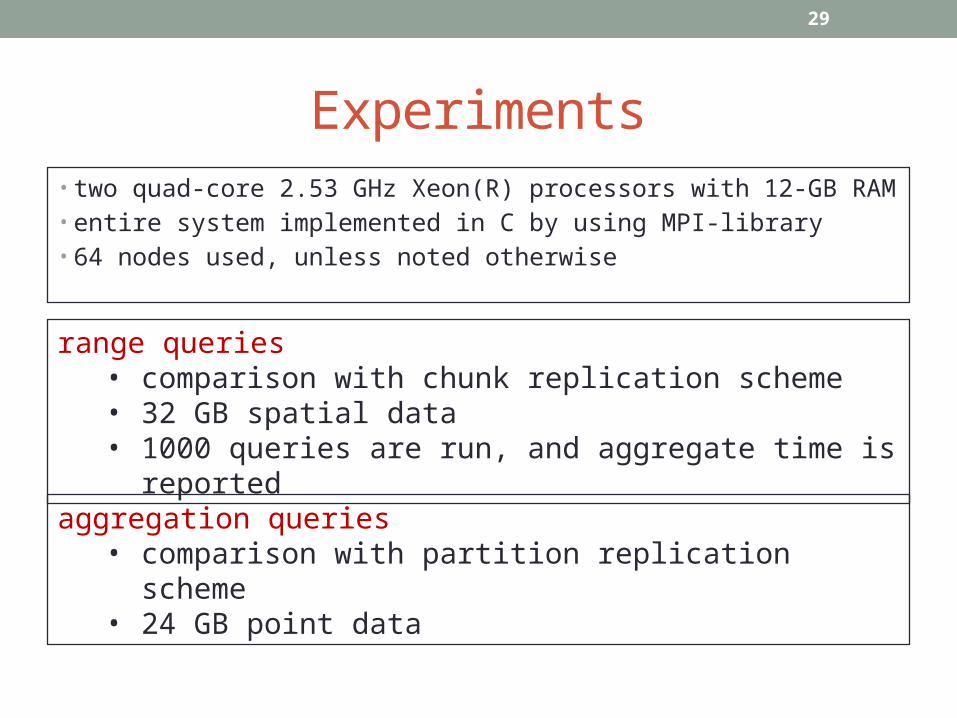
Experiments• two quad-core 2.53 GHz Xeon(R) processors with 12-GB RAM• entire system implemented in C by using MPI-library• 64 nodes used, unless noted otherwise

range queries• comparison with chunk replication scheme• 32 GB spatial data• 1000 queries are run, and aggregate time is reported

aggregation queries• comparison with partition replication scheme• 24 GB point data

30

Experiments: Range Queries

Optimal Chunk Size Selection Scalability

- Execution Times with No Replication and No Failures

* chunk size = 10000

31

Experiments: Range Queries

Single-Machine Failure Rack Failure

- Execution Times under Failure Scenarios (64 workers in total)- k is the number of sub-chunks for a chunk

Future Work

1) Retaining Task-Graph on Data-Flow Models and Experimental Evaluation (continuation of 2nd work)

2) Protection against Soft Errors with DISC Programming Model

Retaining Task-Graph

• Requires knowledge on task-graph structure• efficient detection of producer tasks

• Retain task-graph structure• storing (producer, consumers) per task-level large-space overhead• use a compressed representation of dependencies via iterator-slices• iterator-slice represents a grouping of tasks• An iterator-slice remembers the dependent iterator-slices

Retaining Task-Graph

• Same dependency can be also stored in reverse direction.

a) before data-block has been garbage-collected b) after data-block has been garbage-collected

16-Cases of Recovery• expose all possible cases for recovery• define four dimensions to categorize each data-block

• d1: alive or failed (its producer)

• d2: alive or failed (its consumers)

• d3: alive or failed (where it’s stored)

• d4: true or false (garbage-collected)

<alive,alive,alive,true> <alive,alive,alive,false> <alive,alive,failed,true> <alive,alive,failed,false>

Experimental Evaluation

• Benchmarks to test • LU-decomposition• 2D-Jacobi• Smith-Waterman Sequence Alignment

• Evaluation goals• performance of the model without FT support• space-overhead caused by additional data-structures for FT• Efficiency of proposed schemes under different failure scenarios

Future Work

1) Retaining Task-Graph on Data-Flow Models and Experimental Evaluation (continuation of 3rd work)

2) Protection against Soft Errors with DISC Programming Model

Soft Errors• Increasing soft error rate in current large-systems

• random-bit flips in processing cores, memory, or disk• due to radiation, increasing intra-node complexity, low-voltage

execution, …

• “soft errors in some data-structures/parameters have more impact on the execution than others” (*) • program halt/crash: size and identity of domain, index arrays,

function handles, …• output incorrectness: parameters specific to an application

• ex: atom density, temperature, …

* Dong Li, Jeffrey S. Vetter, Weikuan Yu “Classifying soft error vulnerabilities in extreme-scale applications using a binary instrumentation tool” (SC’12)

DISC model against soft errors• DISC abstractions

• runtime internally maintains critical data-structures• can protect them transparently to the programmer

• protection:1. periodic verification

2. storing in more reliable memory

3. more reliable execution of compute-functions against SDC

Provided Abstraction Data Maintained Internally

Partitioning• number of dimensions• domain/subdomain boundaries• subdomain-to-processor assignment

Communication• interaction parameters (cutoff-radius, point-

connectivity) • low level data (send/receive buffers, buffer sizes)

Computation • pointers to critical functions (compute-function)• core application-state (computation-space)

THANKS!