WHOSE EDUCATION MATTERS IN THE DETERMINATION OFHOUSEHOLD INCOME:

EVIDENCE FROM A DEVELOPING COUNTRY

Dean Jolliffe

FCND DISCUSSION PAPER NO. 39

Food Consumption and Nutrition Division

International Food Policy Research Institute1200 Seventeenth Street, N.W.

Washington, D.C. 20036-3006 U.S.A.(202) 862-5600

Fax: (202) 467-4439

November 1997

FCND Discussion Papers contain preliminary material and research results, and are circulated prior to a fullpeer review in order to stimulate discussion and critical comment. It is expected that most Discussion Paperswill eventually be published in some other form, and that their content may also be revised.

ABSTRACT

This paper aims to answer how best to model education attainment, which is an

individual-level variable, in household-level income functions. The accepted practice in

the literature is to use the education level of the household head. This paper compares the

head-of-household model to three competing models and concludes that the maximum or

average level of education in the household is a better explanatory variable of household

income. Least absolute deviations (LAD) estimators and censored least absolute

deviations (CLAD) estimators are used to predict income. Standard errors, which are

robust to violations of homoscedasticity and independence, are generated by a boot-strap

method that replicates the two-stage sample design.

CONTENTS

Acknowledgments . . . . . . . . . . . . . . . . . . . . . . . . . . . . . . . . . . . . . . . . . . . . . . . . . . . . . v

1. Introduction . . . . . . . . . . . . . . . . . . . . . . . . . . . . . . . . . . . . . . . . . . . . . . . . . . . . . . . 1

2. Data and Descriptive Statistics . . . . . . . . . . . . . . . . . . . . . . . . . . . . . . . . . . . . . . . . . 4

3. Empirical Specification . . . . . . . . . . . . . . . . . . . . . . . . . . . . . . . . . . . . . . . . . . . . . . . 8

Household School Attainment . . . . . . . . . . . . . . . . . . . . . . . . . . . . . . . . . . . . . . . 8Weakest Link—Household Minimum . . . . . . . . . . . . . . . . . . . . . . . . . . . . . 9Talented Tenth—Household Maximum . . . . . . . . . . . . . . . . . . . . . . . . . . 11Household Median and Household Average . . . . . . . . . . . . . . . . . . . . . . . 11

Household Income . . . . . . . . . . . . . . . . . . . . . . . . . . . . . . . . . . . . . . . . . . . . . . . 14Farm Profits . . . . . . . . . . . . . . . . . . . . . . . . . . . . . . . . . . . . . . . . . . . . . . . 14Off-Farm and Total Income . . . . . . . . . . . . . . . . . . . . . . . . . . . . . . . . . . . 16Farm and Off-Farm Labor . . . . . . . . . . . . . . . . . . . . . . . . . . . . . . . . . . . . 18

4. Estimation . . . . . . . . . . . . . . . . . . . . . . . . . . . . . . . . . . . . . . . . . . . . . . . . . . . . . . . 19

Censored Dependent Variables . . . . . . . . . . . . . . . . . . . . . . . . . . . . . . . . . . . . . . 20Outliers and Other Violations of Normality . . . . . . . . . . . . . . . . . . . . . . . . . . . . 21Complex Sample Design . . . . . . . . . . . . . . . . . . . . . . . . . . . . . . . . . . . . . . . . . . 22Independent and Identically Distributed Residuals . . . . . . . . . . . . . . . . . . . . . . . 24LAD and CLAD Estimators . . . . . . . . . . . . . . . . . . . . . . . . . . . . . . . . . . . . . . . . 27

5. Results . . . . . . . . . . . . . . . . . . . . . . . . . . . . . . . . . . . . . . . . . . . . . . . . . . . . . . . . . . 28

Tests of Household School Attainment Models . . . . . . . . . . . . . . . . . . . . . . . . . 29Weakest Link and Household Head Models . . . . . . . . . . . . . . . . . . . . . . . 29Talented Tenth and Household Average Models . . . . . . . . . . . . . . . . . . . . 30

Comparison of Head, Minimum, Average, and Maximum Estimates . . . . . . . . . . 34Gender and Household Schooling . . . . . . . . . . . . . . . . . . . . . . . . . . . . . . . . . . . 37

6. Conclusion . . . . . . . . . . . . . . . . . . . . . . . . . . . . . . . . . . . . . . . . . . . . . . . . . . . . . . . 38

Appendix . . . . . . . . . . . . . . . . . . . . . . . . . . . . . . . . . . . . . . . . . . . . . . . . . . . . . . . . . . . 42

iv

References . . . . . . . . . . . . . . . . . . . . . . . . . . . . . . . . . . . . . . . . . . . . . . . . . . . . . . . . . . 45

TABLES

1. Head of household’s education attainment, intrahousehold comparisons byhousehold size . . . . . . . . . . . . . . . . . . . . . . . . . . . . . . . . . . . . . . . . . . . . . . . . . . . 6

2a. Tests of minimum, average, and maximum schooling: Household incomeand schooling (households with two or more adults) . . . . . . . . . . . . . . . . . . . . . 31

2b. Tests of minimum, median, and maximum schooling: Household incomeand schooling (households with two or more adults) . . . . . . . . . . . . . . . . . . . . . 32

3. Comparison parameter estimates: Household school attainment measuresand household income . . . . . . . . . . . . . . . . . . . . . . . . . . . . . . . . . . . . . . . . . . . . 35

4. Comparison of parameter estimates: Sample design effects and standarderrors, OLS versus LAD . . . . . . . . . . . . . . . . . . . . . . . . . . . . . . . . . . . . . . . . . . 36

5. Tests of joint significance for the gender model (p-values reported) . . . . . . . . . . 38

6. Descriptive statistics . . . . . . . . . . . . . . . . . . . . . . . . . . . . . . . . . . . . . . . . . . . . . 42

7. Household income and household schooling estimates of (1) using allhouseholds with two or more adults . . . . . . . . . . . . . . . . . . . . . . . . . . . . . . . . . . 43

8. Total household income and household schooling: Comparison of household head’sschooling, maximum, and average schooling . . . . . . . . . . . . . . . . . . . . . . . . . . . 44

v

ACKNOWLEDGMENTS

I wish to thank Chris Paxson, Bo Honoré, Cecilia Rouse, Hanan Jacoby, and Paul

Glewwe for comments and advice. In addition, I am grateful for the comments received in

workshops at IFPRI and the World Bank. I would also like to thank Bonnie McClafferty

and Jay Willis for their work in the production of this discussion paper. The paper

expresses my views, which should not be attributed to IFPRI.

Dean JolliffeInternational Food Policy Research Institute

The standard Mincer equation regresses wages on schooling and potential experience (the difference1

between age and schooling, plus six years).

For a discussion of the relative focus of the human capital literature in developing countries, see2

Jolliffe (1996). Good examples of the vastness of the literature on the returns to human capital for wageearners in developing countries are Psacharopoulos (1981), (1985), and (1994).

See World Bank (1995) for a detailed discussion of the typical composition of labor forces in3

developing countries. See Grigg (1991) for more discussion about the predominance of agricultural laborersin developing countries.

1. INTRODUCTION

In developed countries, where the majority of workers are wage earners, the returns

to human capital are typically measured by regressing an individual’s wage on that

individual’s school attainment. The human capital literature for developing countries is1

similarly focused on measuring the returns to education for wage earners, in spite of the

fact that in most of these countries, wage earners are a relatively small fraction of the labor

force. A predominant feature of many developing countries is that the largest share of the2

labor force is engaged in self-employed activities that generate income for

households—either as farm households or as small enterprises. The different composition3

of the labor forces in developed and developing countries has important implications for

the way income data are collected in both types of countries. Income generated from

farming or other household enterprises is almost always measured at the household level,

whereas wage income is uniformly available at the individual level.

2

One exception is a study of 1,904 Korean farm households, in which the household average level of4

education is used as a measure of education attainment for the household. This study is discussed inChapter 4 of Jamison and Lau (1982).

This difference in the way income data are collected makes it difficult to extend the

wage regression model to the developing country context. The difficulty is that in

developing countries, income data are largely measured at the household level, but the

data on education attainment are available at the individual level. As survey data rarely

allow for the decomposition of household income to the individual level, it is not possible

to map an individual’s education attainment to their contribution to household income. A

seemingly natural extension of the wage regression model for this situation would be to

regress the household’s income on the household’s education level. This extension,

though, leads to the difficulty of how to model the household’s education level. The

extension begs the question: whose education matters?

The existing literature only indirectly addresses this issue and answers the question

largely by assuming that only the head of household’s education level matters for the

determination of household income. Jamison and Lau’s (1982) survey of the literature on

schooling and household farm income discusses the results of over 35 studies from Asia,

Africa, and Latin America. With limited exception these studies implicitly assume that it is

only the education level of the head of household that affects farm income and that the

education levels of all other household members have no effect. Similarly studies by Fane4

(1975), Wu (1977), and Jamison and Moock (1984) also use the education level of the

head of household to represent the school attainment for the household, whereas Huffman

3

Fane’s and Huffman’s studies used U.S. farm households. Jamison and Moock look at Nepalese farm5

households, and Wu examines Taiwanese farm households. Lin examines whether education affects theadoption of new technologies in the Hunan Province of China.

In the case of Ghana, 47 percent of the households generate some self-employed, off-farm income,6

while 36 percent of the households have at least one wage-earning member. Similarly, the average value ofself-employed, off-farm income is 225 percent greater than the average household income generated fromwage employment. Vijverberg (1991a, 2) also notes that, “family enterprises with one to four workersaccounted for about 70 percent of manufacturing in India and Indonesia, 60 percent in the Philippines, and40 percent in Korea and Columbia.”

(1974) uses the education levels of the head of household and spouse and Lin (1991) uses

both head of household and average household level of education.5

Another important component of household income in many developing countries is

self-employed, off-farm income. This component of household income has been widely

ignored in the human capital literature, even though self-employed, off-farm income is at

least as significant as wage income in many developing countries. Vijverberg’s (1991a)6

study is one of few papers on returns to human capital that examines self-employed, off-

farm work. He uses the education level of the operator of the household enterprise as the

measure of education for the enterprise.

The practice of using the school attainment of only one household member

implicitly assumes that the education level of all other household members is irrelevant.

While this assumption is pervasive, it may not be reasonable. Consider two households,

one in which no one has any schooling and the other in which the head has no schooling,

but all other members have completed secondary schooling. The standard assumption

implies that these two households possess the same amount of human capital.

4

The purpose of this paper is to empirically consider three models of household

education, and determine whether the intrahousehold allocation of education matters in

the determination of household income. The plan of this paper is as follows. Section 2

discusses the data used in this paper and presents a few descriptive statistics on headship

in Ghana and labor activities of Ghanaian households. Section 3 presents three simple

paradigms of whose education matters in regression models of household income. This

section also describes the composition of household income, and proposes the appropriate

explanatory variables for estimation. Section 4 describes the estimation methodology.

Consistent estimates for the farm and off-farm income functions are obtained by using

Powell’s (1984) censored least absolute deviations (CLAD) estimators. Consistent

standard errors are obtained by using a bootstrap methodology that mimics the two-stage

sample design. Section 5 contains a summary of the estimation results. Most notably, the

results suggest that using either the maximum or average level of schooling in the

household (rather than the education level of the head of household) provides a more

accurate measure of the return to education. Section 6 provides some concluding

comments.

2. DATA AND DESCRIPTIVE STATISTICS

The data used in this paper are from the Ghana Living Standards Survey (GLSS), a

nationwide household survey carried out by the Ghana Statistical Service with technical

assistance from the World Bank. The survey, administered from October 1988 to

5

Five households are missing school data, and 33 households are missing agricultural price data.7

September 1989, covers 3,200 households and contains detailed information on formal

and informal labor activities, household farm activities, expenditures, education status of

household members, and many other determinants of household welfare. (See Glewwe

and Twum-Baah [1991] for more information.) A supplemental education module was

also administered to a nationally representative subsample of 1,585 households. This

paper uses the data from the subsample of 1,585 households. Thirty-eight of these

households are dropped due to missing data, resulting in a sample of 1,547 households.7

In the GLSS data, as with many household surveys, the head of household title is a

self-ascribed characteristic. As the definition of head of household varies across cultures

and across surveys, it is likely to be an unreliable characteristic for cross-survey

comparisons. Similarly, if the concept of headship varies across households within Ghana

or if headship is based not on education attainment or management skills but on age, for

example, then the headship model is likely to mismeasure the returns to education for the

household.

Using the education level of the head would be a more tenable assumption if

headship were correlated with the education level in the household. In this case, it could

be argued that headship is assigned to those with the most (or close to the most)

education, because they will make the best decisions for the household. In the GLSS data,

the head of household’s education level is often the highest in the household, but it is also

frequently the lowest. Table 1, below, presents the percentage of households in which the

6

The table actually lists households by the number of household members over the age of 15.8

Throughout this paper, all education attainment variables are only for individuals over the age of 15. Thisis to ensure that the majority of continuing students are not included in the analysis.

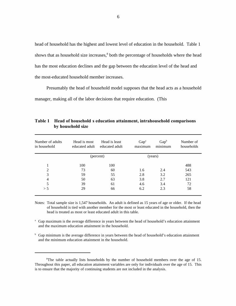
head of household has the highest and lowest level of education in the household. Table 1

shows that as household size increases, both the percentage of households where the head8

has the most education declines and the gap between the education level of the head and

the most-educated household member increases.

Presumably the head of household model supposes that the head acts as a household

manager, making all of the labor decisions that require education. (This

Table 1—Head of household’s education attainment, intrahousehold comparisonsby household size

Number of adults Head is most Head is least Gap Gap Number ofa b

in household educated adult educated adult maximum minimum households

(percent) (years)

1 100 100 4882 73 60 1.6 2.4 5433 59 55 2.8 3.2 2654 50 63 3.8 2.7 1215 39 61 4.6 3.4 72

> 5 29 66 6.2 2.3 58

Notes: Total sample size is 1,547 households. An adult is defined as 15 years of age or older. If the headof household is tied with another member for the most or least educated in the household, then thehead is treated as most or least educated adult in this table.

Gap maximum is the average difference in years between the head of household’s education attainmenta

and the maximum education attainment in the household.

Gap minimum is the average difference in years between the head of household’s education attainmentb

and the minimum education attainment in the household.

7

assumes that it is only the decisions, and not the implementation, that require human

capital.) This model is most credible in the context of a household in which all members

are working on the same task, such as farming. The assumptions of the model seem less

tenable as households engage in additional income-generating activities. This is because

the monitoring demands on the manager are likely to dramatically increase when parts of

the household are working on the farm, while other household members are working off

of the farm.

In the case of Ghana, there is a great amount of diversity in labor activities. There

are 3,698 laborers in this sample of 1,547 households. Of these individuals, 77 percent

spend some time working on a farm and 56 percent spend some time engaged in some

other form of labor. Thirty-four percent of the individuals are engaged in both some

farming and nonfarming activities. The extent of the labor diversification increases when

considering all labor within the household. In 55 percent of the households, at least one

person has spent some time working on a farm and at least one person has spent some

time in nonfarm labor. This level of labor diversity further suggests that the assumptions

of the head of household model are difficult to support.

The human capital literature for developing countries estimates the returns to

education by either estimating a Mincer-type wage equation or by estimating some form of

a farm production or profit function. Without exception, the literature assumes that

individuals or farm households are engaged in only one income-generating activity.

Because so many households and individuals are engaged in more than one income-

8

generating activity, estimating the returns to education by focusing on either strictly farm

income or wage income will provide an incomplete picture of the importance of education.

For this reason, this paper examines total household income, farm household income, and

off-farm household income.

3. EMPIRICAL SPECIFICATION

This section first lays out a general specification of the household’s school

attainment, which captures much of the information on the household’s distribution of

schooling. Following this is a description of three basic paradigms of how to model

household school attainment. The testable implications of these models of household-level

school attainment are also described. This section finishes with a brief explication of how

total household income and its components are calculated.

HOUSEHOLD SCHOOL ATTAINMENT

In order to answer the question of whose education matters for the determination of

household income, this paper first considers a basic specification that includes the

minimum, average, and maximum value of school attainment from the distribution of

schooling within each household. The three models tested alternatively assume that one of

these terms is a determinant of household income, while the other two have no effect on

household income. The model is then extended in two ways. First, the education level of

the head of household is also included (along with minimum, average, and maximum

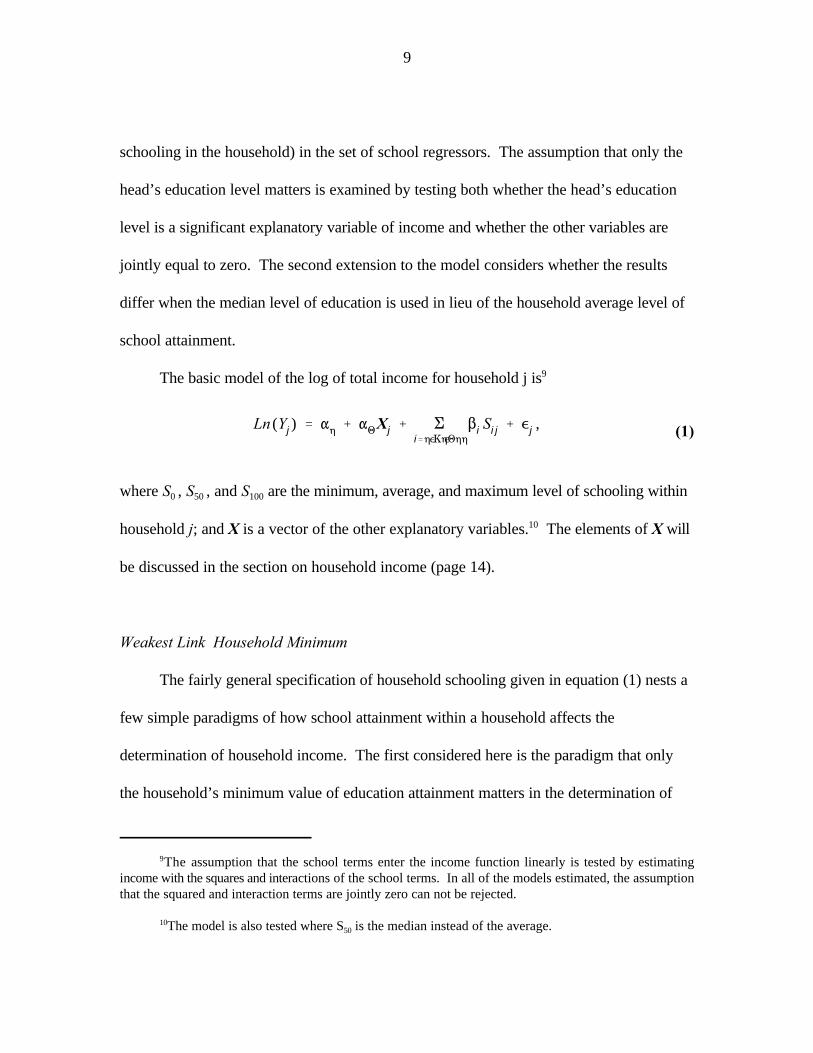
Ln (Yj) ' "0 % "1Xj% Ei'0,50,100

$iSij% ,j,

9

The assumption that the school terms enter the income function linearly is tested by estimating9

income with the squares and interactions of the school terms. In all of the models estimated, the assumptionthat the squared and interaction terms are jointly zero can not be rejected.

The model is also tested where S is the median instead of the average.1050

(1)

schooling in the household) in the set of school regressors. The assumption that only the

head’s education level matters is examined by testing both whether the head’s education

level is a significant explanatory variable of income and whether the other variables are

jointly equal to zero. The second extension to the model considers whether the results

differ when the median level of education is used in lieu of the household average level of

school attainment.

The basic model of the log of total income for household j is9

where S , S , and S are the minimum, average, and maximum level of schooling within0 50 100

household j; and X is a vector of the other explanatory variables. The elements of X will10

be discussed in the section on household income (page 14).

Weakest Link–Household Minimum

The fairly general specification of household schooling given in equation (1) nests a

few simple paradigms of how school attainment within a household affects the

determination of household income. The first considered here is the paradigm that only

the household’s minimum value of education attainment matters in the determination of

10

When considering households with more than one member over the age of 15, the percentage of11

households where the head has the least amount of education drops to about 60 percent.

For example, those individuals between the ages of 15 and 44 have, on average, 6.6 years of12

schooling, while those 45 years of age and older have, on average, 2.2 years of education. (The t-statistic forwhether these averages are different is 26.4.) See Jolliffe (1996) for a breakdown of education attainment byage and sex.

household income. This model is motivated by the popular management aphorism that a

production process is only as good as its weakest link. The notion is that one bad input or

one mistake will ruin the entire product. This model is most likely to be appropriate for

production processes that are highly sensitive to mistakes.

Of the three paradigms considered in this paper, the weakest link most closely

resembles the head of household model, at least in the case of Ghana, where in 70 percent

of the households, the head has the lowest level of education. In Ghana, the elderly have11

the least amount of education, and it is quite common for the oldest person in the12

household to be designated the head by the household. In 91 percent of the GLSS

households, headship is ascribed to the oldest member in the house.

If the weakest link paradigm is the correct model, then there are two testable

implications from estimating equation (1). The first is that the parameter estimates on the

average and maximum level of schooling, $ and $ , are jointly equal to zero. The50 100

second implication is that the parameter on the minimum level of schooling, $ , is nonzero. 0

11

The talented tenth nomenclature is taken from a model of macroeconomic development proposed by13

W.E.B. Du Bois for the black community in America. Du Bois believed that the path to improved livingstandards for African-Americans would be best attained by educating a small elite group of African-Americans, who would then be able to lead the rest of their community into prosperity. The use of this nameis only meant to evoke the idea of investing all of the education resources into a few individuals who wouldthen help out the others. It is not intended to suggest that Du Bois proposed this idea as a theory ofintrahousehold allocation of education.

Talented Tenth – Household Maximum

Another paradigm considered in this paper is that only the household’s maximum

value of education attainment matters in the determination of household income. This

model is motivated by the notion that one well-educated member of the family can make

the business decisions requiring the skills acquired in schools and can partake in the most

intellectually demanding activities. In some ways, this may be the model many have in13

mind when using the education level of the head of household.

If the talented tenth paradigm is the correct model, there are two testable

implications that are very similar to those for the weakest link model. The implications are

that the parameter estimates from estimating equation (1) on the minimum and median

level of schooling, $ and $ , are jointly equal to zero, while the term for the maximum0 50

level of schooling, $ , is nonzero. 100

Household Median and Household Average

The final paradigm of how household school attainment affects household income is

that a midpoint value of the household’s school attainment is the important determinant of

household income. To test this, both the average and median values of schooling are used

12

for the S variable. The motivation for this model is that the skills of all workers are50

important for the creation of household income, and one good manager or one weak link

is not the driving force. While the median and the average values of school attainment are

very similar, the estimation results differ slightly and a summary of both are presented.

If the household average or median paradigm is the correct model, there are again

two similar sets of testable implications. The first is that the parameter estimates on the

minimum and maximum level of schooling, $ and $ , are jointly equal to zero. The0 100

second implication is that the parameter on the average or median level of schooling, $ ,50

is nonzero.

One important assumption placed on the way schooling is specified in all three

models is that households cannot hire-in educated laborers. In other words, the market

for educated laborers is imperfect and households are unable to purchase the profit-

maximizing level of schooling by hiring in educated managers. There is some evidence in

the GLSS data that suggests that markets for educated laborers are not very active and

that this assumption is reasonable. For example, the average Ghanaian farm household

spends less than 5 percent of farm income on hiring in labor. Of the labor that is hired-in,

70 percent of the wages go for clearing land—presumably not an education-intensive job.

One problem in estimating the models of school attainment is that they require

regressing household income on three measures of school attainment that are highly

correlated. This is primarily the case because there are numerous households with only

one or two adult members. In households with only one adult member, the minimum,

13

Only the estimation results from using the sample of households with two or more households are14

presented in this paper. The results from using all households and households with three or more adults arequalitatively similar and are presented in full in Jolliffe (1996).

Households with more female members have, on average, lower levels of schooling because females15

attain less education than males, on average. Households with more females are also likely to engage indifferent types of labor, which will affect farm and off-farm income differently. In particular, females are morelikely to engage in work that does not generate income as measured by the GLSS survey, such as housework.These gender effects are likely to be both correlated with income levels and schooling, and unless controlledfor, will bias the estimated effect of schooling on income.

The similarity is that higher levels of cognitive skills and schooling both increase household off-farm16

income by much more than they increase farm income.

average, and maximum level of school attainment will all be the same value. In order to

reduce the level of correlation across the variables, all models are estimated over three

samples: (1) all households, (2) all households with two or more adult members, and

(3) all households with three or more adult members. 14

It is important to also note that human capital is a complex, multidimensional

characteristic, and school levels will capture certain aspects of it, but are also likely to

confound human capital with other characteristics such as wealth or innate ability. These

issues are only dealt with in this paper to a limited extent. For example, to control for

some forms of omitted variable bias, the regression models include household composition

variables and some information on household assets. The household composition

variables will control for differences in education levels that are correlated with income

levels but are due to gender differences. To control for the possibility that schooling15

may not measure human capital at all, this paper refers to Jolliffe (1996), which uses a

different measure of human capital (cognitive skills) and finds that the returns to skills are

positive and similar to the returns from schooling. 16

14

To correct for an inflation rate of 24 percent during the year of fieldwork (Ghana Statistical Service17

1991a), all values are converted to constant cedis (C/ ), with the base month as October 1988. The averageexchange rate during 1988 was C/ 200 to US$1 (Ghana Statistical Service 1991b).

The difficulties associated with using school attainment to measure human capital

are substantial, so it is worthwhile to note that the purpose of this paper is not to measure

the returns to human capital. Rather this paper compares different measures of household

school attainment to determine which measures best explain income, and also to determine

if the standard practice of using the head of household’s schooling as the measure of the

household’s total level of schooling is valid.

HOUSEHOLD INCOME

To test the three paradigms discussed above, this paper estimates three separate

household income functions—total income, farm income, and off-farm income. This

strategy explicitly acknowledges that many households are engaged in numerous income-

generating activities, and while a household member’s education level may not matter for

the determination of income in one activity, it may matter for another. Below is a

description of the components of total household income.

Farm Profits

Farm output is measured as the value of all crops and animal products marketed in

the last 12 months plus the value of crops kept for seed and given away as gifts. 17

15

In Ghana, the GLSS data indicate that the value of home-consumed crops constitutes 62 percent of18

the total value of farm output. Crops sold on the market contribute to 35 percent of the total farm output, andthe remaining 3 percent comes from the sale and home consumption of animal products.

In the Type I Tobit model, the zeros are typically explained by an optimization problem which results19

in a negative value for the desired level of the dependent variable. This estimation problem perhaps morenaturally falls into the Type II Tobit, or selection model framework. In the Type II framework, the zeros existbecause some households choose not to be farmers. The Type I Tobit framework is chosen for this paper dueto a lack of a credible model defining the selection process into (or out of) farming.

Because many farmers cover their subsistence needs from their own production, the

estimated value of home consumption of food and animal products is also included in the

measure of total farm output. Subtracted from this measure of farm output are18

expenditures on seed, fertilizer, insecticide, pesticide, livestock, storage, transportation,

rented-in land, and hired-in labor. Crops given as payments for other inputs are also

subtracted from the value of farm output. The resulting figure is a measure of profit,

conditional on the quantity of land and labor. (The value of one is added to farm profit to

allow the log transformation of farm profit.) The log of farm profit is modeled as a Type 1

Tobit model:19

ln (Y + 1) = ln Y (A , L , p S, µ) (2)f f f f* *

f

ln (Y +1) = ln (Y + 1) if Y + 1 > 1f f f* *

= 0 if Y +1 # 1 ,f*

16

Throughout this paper the subscript f will denote a farm variable and the subscript o will denote an20

off-farm variable. These subscripts will only be used on variables which could pertain to either farm or off-farm activities. The subscripts denoting household- and individual-level characteristics previously used aredropped here for clarity.

Land is treated throughout this paper as a fixed input. In an economy where land markets function21

well, treating land as fixed would be inappropriate. The more appropriate strategy would be to treat land likeany other input: subtract the rental value of land from total output and include the rental price of land in theset of regressors. In the case of Ghana, though, it is difficult to establish a reasonable rental value for theland. Only 17 percent of the farmers rent any land in or out and land is rarely sold, both of which mean thatland rental prices are not well defined. The fact that land rental markets are not very active suggests, though,that treating land as a fixed input may not be a too egregious assumption.

The p vector contains cluster average prices for maize, okra, cassava, and pepper crops as well as22f

the cluster average input prices for fertilizer and insecticide.

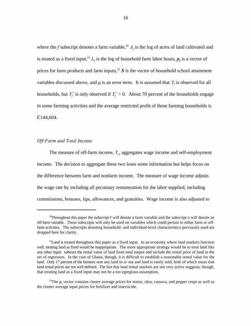
where the f subscript denotes a farm variable, A is the log of acres of land cultivated and20f

is treated as a fixed input, L is the log of household farm labor hours, p is a vector of21f f

prices for farm products and farm inputs, S is the vector of household school attainment22

variables discussed above, and µ is an error term. It is assumed that Y is observed for allf

households, but Y is only observed if Y > 0. About 70 percent of the households engagef f* *

in some farming activities and the average restricted profit of those farming households is

C/ 144,604.

Off-Farm and Total Income

The measure of off-farm income, Y , aggregates wage income and self-employmento

income. The decision to aggregate these two loses some information but helps focus on

the difference between farm and nonfarm income. The measure of wage income adjusts

the wage rate by including all pecuniary remuneration for the labor supplied, including

commissions, bonuses, tips, allowances, and gratuities. Wage income is also adjusted to

17

reflect the value of all nonpecuniary payments, including remuneration in the form of food,

crops, animals, housing, clothing, transportation, or any other form.

The measure of off-farm, self-employed income is recommended by Vijverberg

(1991b) and is the reported amount of money left over from self-employed business

activities after expenses have been incurred. This measure has the advantage of resulting

in strictly nonnegative values.

The log of off-farm income is also modeled as a Type I Tobit:

ln (Y + 1) = ln Y (A , L , S, g) (3)o o o o* *

ln (Y + 1) = ln (Y + 1) if Y + 1 > 1o o o* *

= 0 if Y + 1 # 1 ,o*

where the o subscript denotes an off-farm variable, A is the log of business assets ando

years of work experience, L is the log of household off-farm labor hours, S is the vectoro

of household school attainment variables discussed above, and g is an error term. It is

assumed that Y is observed for all households, but Y is only observed if Y > 0. (Theo o o* *

value of one is also added to off-farm income to allow the log transformation of farm

profit.) About 67 percent of the households have at least one household member who

engages in some form of off-farm work, and the average off-farm income for these

households is C/ 373,143. Total household income is modeled simply as the sum of farm

and off-farm income. The average value of total household income is C/ 326,743.

18

The relative productivity in the farm and off-farm activities is measured by wages in the two sectors.23

The measure of farm wages used is the wages for an adult male, day laborer. The measures of off-farm wagesare representative of the wages faced by the sample, yet are drawn from an independent sample. Thesupplemental education module was included for only a randomly selected half of the total sample. From thehalf that did not receive the supplemental module, an hourly wage for all off-farm work was calculated andthen grouped by occupation types. From these occupation groupings, which are representative of the off-farmwork of the tested sample, mean wages by regions are calculated and then used as estimates of the off-farmwages faced by the sample.

Gender composition is also included, as there are cultural norms that dictate that men, women, and24

children will typically perform different work activities; and, often times, the activities of the women andchildren will not be picked up in the measure of off-farm work. For example, the time spent collectingfirewood or food preparation is not included in the measure of total hours worked.

Farm and Off-Farm Labor

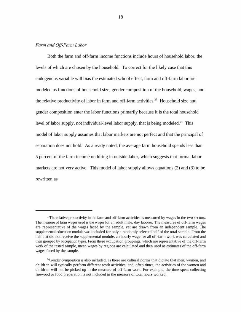
Both the farm and off-farm income functions include hours of household labor, the

levels of which are chosen by the household. To correct for the likely case that this

endogenous variable will bias the estimated school effect, farm and off-farm labor are

modeled as functions of household size, gender composition of the household, wages, and

the relative productivity of labor in farm and off-farm activities. Household size and23

gender composition enter the labor functions primarily because it is the total household

level of labor supply, not individual-level labor supply, that is being modeled. This24

model of labor supply assumes that labor markets are not perfect and that the principal of

separation does not hold. As already noted, the average farm household spends less than

5 percent of the farm income on hiring in outside labor, which suggests that formal labor

markets are not very active. This model of labor supply allows equations (2) and (3) to be

rewritten as

19

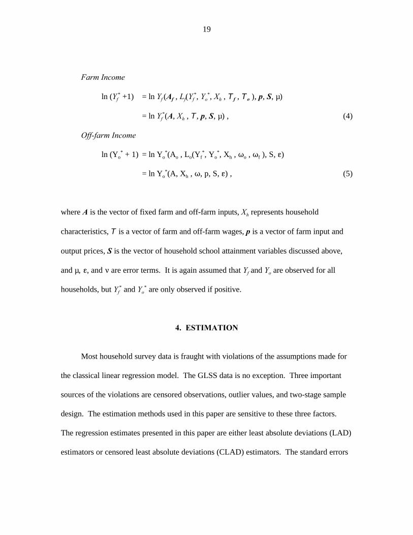
Farm Income

ln (Y +1) = ln Y (A , L (Y , Y , X , T , T ), p, S, µ)f f f f o h* * *

f f o

= ln Y (A, X , T, p, S, µ) , (4)f h*

Off-farm Income

ln (Y + 1) = ln Y (A , L (Y , Y , X , T , T ), S, g)o o o o f o h o f* * * *

= ln Y (A, X , T, p, S, g) , (5)o h*

where A is the vector of fixed farm and off-farm inputs, X represents householdh

characteristics, T is a vector of farm and off-farm wages, p is a vector of farm input and

output prices, S is the vector of household school attainment variables discussed above,

and µ, g, and < are error terms. It is again assumed that Y and Y are observed for allf o

households, but Y and Y are only observed if positive. f o* *

4. ESTIMATION

Most household survey data is fraught with violations of the assumptions made for

the classical linear regression model. The GLSS data is no exception. Three important

sources of the violations are censored observations, outlier values, and two-stage sample

design. The estimation methods used in this paper are sensitive to these three factors.

The regression estimates presented in this paper are either least absolute deviations (LAD)

estimators or censored least absolute deviations (CLAD) estimators. The standard errors

20

This decision is made because it is difficult to find variables that explain why a household engages25

in farming, but that have no effect on the households farming abilities. This is particular true in a country likeGhana, where movement between farm and off-farm activities is fairly fluid, and so many households areengaged in both activities.

used for these estimators are bootstrap estimates, which are derived by replicating the

two-stage sample design.

CENSORED DEPENDENT VARIABLES

Roughly 70 percent of all Ghanaian households are engaged in farming activities,

and similarly about 67 percent of the households generate some of their household income

from off-farm activities. The strategy used in this paper avoids modeling the selection rule

determining who farms and who does not, and simply treats farm and off-farm income as

data that are censored at zero. 25

The problem introduced by censoring is that OLS results in biased estimators, and

the standard Tobit or Heckman estimators for censored models rely heavily on the

assumption of normality. Arabmazar and Schmidt (1981) show that the bias resulting

from the Tobit estimator in the presence of heteroscedastic residuals can be quite large.

Vijverberg (1987) presents similar results showing that the bias of the Tobit estimator is

quite large when kurtosis and skewness are nonnormal. Powell’s CLAD estimator results

in consistent estimates for the limited dependent variable model in the presence of many

violations of normality, including heteroscedasticity.

21

Often times, one or two large outliers are enough to significantly affect the skewness. The assumption26

that kurtosis is near 3, which is indicative of normality, is also typically violated, because the number ofrelatively extreme values is large. (In other words, the tails of the distribution are typically ‘thicker’ than thoseof the normal distribution.)

The value of kurtosis is 10.4 for the residuals. The Shapiro-Francia (1972) test of normality for the27

residuals from predicting the log of total income results is a Z-statistic of 9.6, which has a p-value ofapproximately zero.

OUTLIERS AND OTHER VIOLATIONS OF NORMALITY

A standard feature of many household data sets is the presence of unusually large or

small values. In addition to outliers, the skewness and kurtosis of the data will often

exhibit nonnormal characteristics. When the dependent variable in a model contains26

outlier values or is nonnormally distributed, it is likely that the resulting residuals will be

nonnormally distributed. Consider, for example, the total income variable used in this

paper. The mean value for total household income is C/ 326,743, the standard error of total

income is ten times this size, and the maximum value is C/ 140,000,000. The residuals from

estimating the log of total household income, exhibit large values of kurtosis and strongly

violate the assumption of normality.27

It is these characteristics that frequently lead either the statistical agency that

collected the data or the researcher using the data to arbitrarily dispense of observations

that seem incredibly large or small. Often the rules used to include or exclude variables

are based on some prior belief that the data should be normally distributed. The

advantage of the LAD and CLAD estimators used in this paper is that they are less

sensitive to outliers than OLS and are robust to violations of kurtosis. For this reason, no

extreme data points are excluded from the sample and arbitrary selection rules are

22

The systematic aspect of the sample design results in a sample that is stratified on geographic28

(coastal, forest, and savannah) and urban/rural regions. The stratification ensures that the sample is inproportion to the population of the strata. Stratification will also reduce sampling error to the extent that thecharacteristics defining the strata are correlated with the variables of interest. (For more details on the sampledesign, see Scott and Amenuvegbe 1989.)

Fewer than 200 unique clusters were selected because once a cluster was selected, it was returned to29

the pool of candidate clusters. Selection with replacement allows for the possibility that certain clusters willbe selected more than once.

In the case of Ghana, 16 households were selected from within each cluster. If the same cluster was30

chosen twice, for example, then 32 households were selected. Household selection, in contrast to clusterselection, was not done with replacement.

avoided. The LAD estimators are less sensitive to outliers than OLS because it is the

distance from the median and not the square of the distance (from the average) that

determines the parameter estimates. (This is analogous to the fact that medians are less

sensitive to outliers than are means.)

COMPLEX SAMPLE DESIGN

As with essentially all nationwide household surveys, the design of the GLSS

sample is not a simple random draw of households. The GLSS sample design is a two-

stage, systematic design, which results in a clustered and stratified sample. The two-28

stage aspect of the design entailed first dividing Ghana into numerous clusters or

geographic regions and assigning to each cluster a weight that was proportional to the

population residing within the cluster. Then using these weights, approximately 200

clusters were randomly chosen. The second stage of the sample selection process29

randomly selects a fixed number of households within each cluster. 30

23

For a more detailed discussion about the advantages and disadvantages, as well as the estimation31

implications, of complex survey designs, see Howe and Lanjouw-Olson (1995).

Scott and Holt (1982) for example, discuss the impact of sample design on the correction required32

for the OLS standard errors. Arabmazar and Schmidt (1981) show that when complex sample designs resultin heteroscedasticity, that standard limited dependent variable estimators (including the Tobit and Heckman’stwo-step procedure) are significantly biased.

The advantages of a clustered, two-stage sample design are purely practical. By

using a clustered design, the interview teams are required to cover less territory and the

cost of the survey is dramatically reduced. A disadvantage of the clustered design is that

clustering will typically result in higher estimated variances than the same number of

observations from a purely random sample. Another more generic and important

disadvantage of complex designs is that analytical standard errors can become difficult to

calculate.31

The primary concern with data from a two-stage sample design is that it is likely to

result in residuals that are neither homoscedastic nor independently distributed. This is

because households within a specific cluster are likely to be more similar to each other

than to households in other clusters. The result of this is that intracluster variation is likely

to be significantly different from inter-cluster variation of the residuals. Numerous papers

illustrate that these violations can have large effects on estimated parameters and standard

errors, and it is now being somewhat more widely recognized in the economics literature

that correcting for these violations are important for generating credible results. This32

section proceeds by examining whether the residuals from estimating total household,

farm, and off-farm income exhibit heteroscedasticity and dependence.

24

The p-value of the statistic is essentially zero. The test statistic is equal to 560, which is distributed33

as a P with 60 degrees of freedom.2

The p-value of both of these test statistics are zero. The test statistics are 1,152.5 and 108.6 for the34

farm and off-farm functions, respectively. Both statistics are distributed as a P with 60 degrees of freedom.2

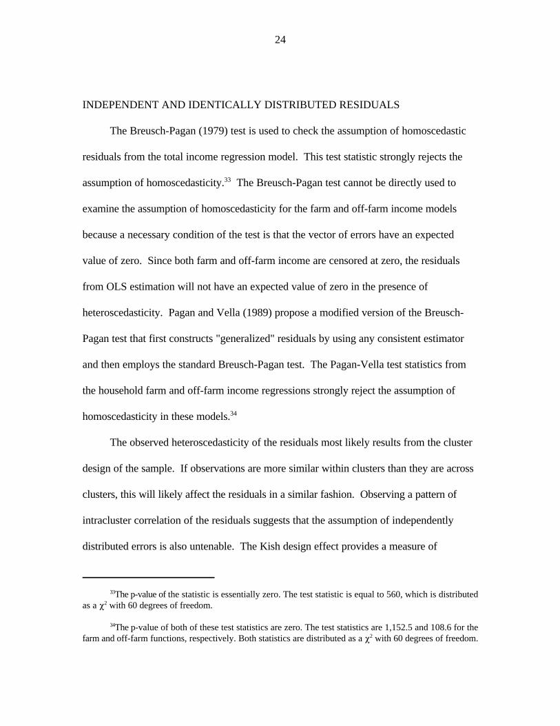
INDEPENDENT AND IDENTICALLY DISTRIBUTED RESIDUALS

The Breusch-Pagan (1979) test is used to check the assumption of homoscedastic

residuals from the total income regression model. This test statistic strongly rejects the

assumption of homoscedasticity. The Breusch-Pagan test cannot be directly used to33

examine the assumption of homoscedasticity for the farm and off-farm income models

because a necessary condition of the test is that the vector of errors have an expected

value of zero. Since both farm and off-farm income are censored at zero, the residuals

from OLS estimation will not have an expected value of zero in the presence of

heteroscedasticity. Pagan and Vella (1989) propose a modified version of the Breusch-

Pagan test that first constructs "generalized" residuals by using any consistent estimator

and then employs the standard Breusch-Pagan test. The Pagan-Vella test statistics from

the household farm and off-farm income regressions strongly reject the assumption of

homoscedasticity in these models.34

The observed heteroscedasticity of the residuals most likely results from the cluster

design of the sample. If observations are more similar within clusters than they are across

clusters, this will likely affect the residuals in a similar fashion. Observing a pattern of

intracluster correlation of the residuals suggests that the assumption of independently

distributed errors is also untenable. The Kish design effect provides a measure of

1 %En 2

c i

n&1

EcEiEj…1

(xci&x)(xc j&x)

F̂2Ecnc(nc&1)

25

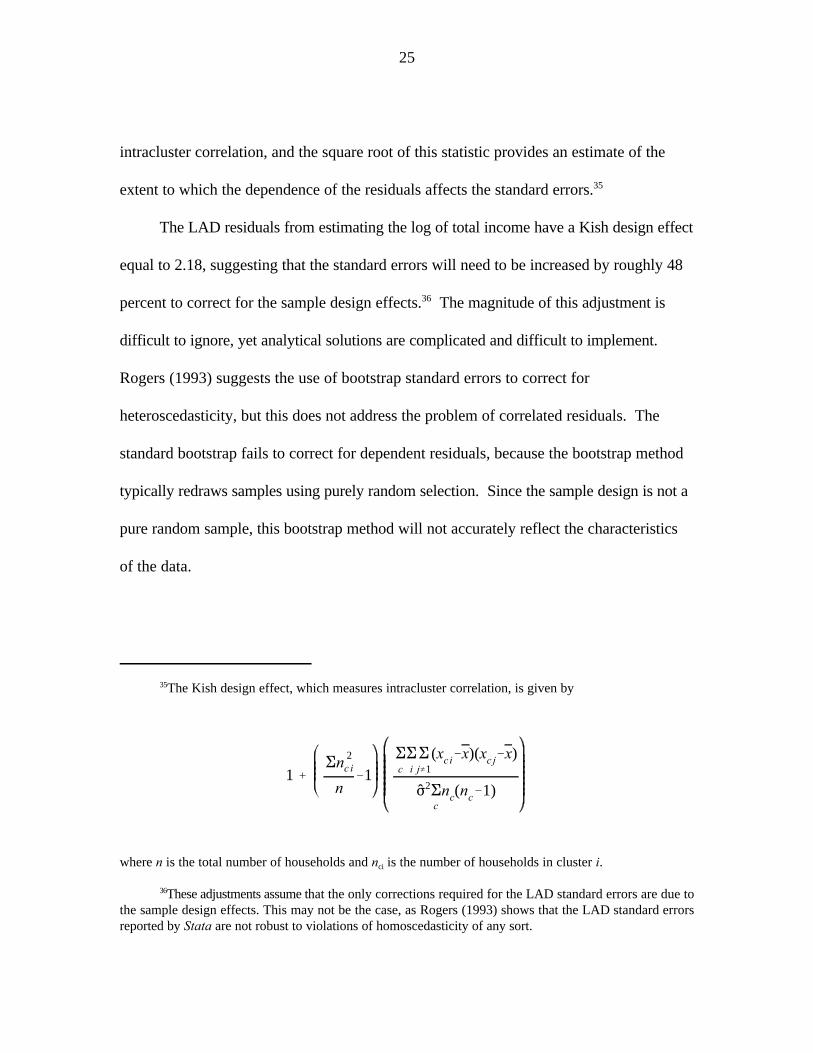
The Kish design effect, which measures intracluster correlation, is given by35

where n is the total number of households and n is the number of households in cluster i.ci

These adjustments assume that the only corrections required for the LAD standard errors are due to36

the sample design effects. This may not be the case, as Rogers (1993) shows that the LAD standard errorsreported by Stata are not robust to violations of homoscedasticity of any sort.

intracluster correlation, and the square root of this statistic provides an estimate of the

extent to which the dependence of the residuals affects the standard errors.35

The LAD residuals from estimating the log of total income have a Kish design effect

equal to 2.18, suggesting that the standard errors will need to be increased by roughly 48

percent to correct for the sample design effects. The magnitude of this adjustment is36

difficult to ignore, yet analytical solutions are complicated and difficult to implement.

Rogers (1993) suggests the use of bootstrap standard errors to correct for

heteroscedasticity, but this does not address the problem of correlated residuals. The

standard bootstrap fails to correct for dependent residuals, because the bootstrap method

typically redraws samples using purely random selection. Since the sample design is not a

pure random sample, this bootstrap method will not accurately reflect the characteristics

of the data.

26

The number of selected households is equal to the total number of households that are in the cluster.37

Similarly, the number of clusters chosen from each strata is equal to the number of clusters that belong in eachstrata. The random selection is with replacement, so a given household or cluster may be represented morethan once in any of the bootstrapped samples.

The LAD estimates presented in this paper come from Stata’s qreg command, which follows Koenker38

and Bassett in deriving its estimates. Rogers (1993) shows that the standard errors reported by Stata are notrobust to violations of homoscedasticity or independence. The standard errors presented in this paper arederived from the stratified, two-step bootstrap procedure described above.

In order to correct for both heteroscedasticity and the dependence of the residuals,

this paper uses a bootstrap procedure that replicates the sample design. The bootstrap

resamples the data using a two-stage procedure, which is also stratified on the three

geographic regions of Ghana as well as the urban/rural split. In the first stage, clusters are

randomly selected from each of the six strata. In the second stage, a fixed number of

households are selected in each cluster. Using this method, each household does not37

have an equal probability of being chosen; rather, there is a dependence created in the re-

sampling such that if one household is selected in a cluster, then the probability of

selection for the other households in that cluster increases. By following this method, the

redrawn samples exhibit the same characteristics as the initial sample, and the estimated

standard errors are robust to violations of both homoscedasticity and independence.

LAD AND CLAD ESTIMATORS

To estimate total household income, this paper uses the LAD estimator. The

properties of this estimator are presented in Koenker and Bassett (1978). The LAD38

estimator is found by minimizing

27

More generally, observations are dropped if the predicted value is less than the censoring value when39

the left tail of the distribution is censored. Similarly, observations are dropped if the predicted value is greaterthan the censoring value when the right tail of the distribution is censored.

3 | y - x ' $ | . (6)i i

To estimate farm and off-farm income, both of which are censored at zero, this paper uses

Powell's (1984) CLAD estimator. This estimator provides consistent estimates for the

censored model when heteroscedasticity is present, as well as other violations of

normality. The CLAD estimator is found by minimizing

3 | y - max(0, x ' $) | . (7)i i

The consistency of this estimator rests on the fact that medians are preserved by monotone

transformations of the data, and equation (7) is a monotone transformation of equation

(6), the standard median regression.

The estimation technique used in this paper for the CLAD estimator is Buchinsky’s

(1994) iterative linear programming algorithm (ILPA). The first step of the ILPA is to

estimate a quantile regression for the full sample, then delete the observations for which

the predicted value of the dependent variable is less than zero. Another quantile39

regression is estimated on the new sample, and again negative predicted values are

28

Converges occur when there are no negative predicted values in two consecutive iterations. All of40

the models estimated in this paper converged, and, typically, converged in fewer than 15 iterations.

The models are tested over three samples—all households, households with two or more adults, and41

households with three or more adults. Only the results from using the sample with two or more adults arepresented in this paper. The estimation results from the other two samples are qualitatively similar and arepresented in Jolliffe (1996).

dropped. Buchinsky (1991) shows that if the process converges, then a local minimum is40

obtained.

5. RESULTS

This section first summarizes the results from testing the weakest link, talented

tenth, household head, and household average models of school attainment. Each of the

models is tested for the three measures of household income (total, farm, and off-farm). 41

This section then summarizes results from estimating household income separately, using

the maximum, average, and household head’s level of school attainment. In addition to

comparing the differences in the estimated effects of school attainment from using

different measures of school attainment, this section discusses the differences between

OLS and LAD estimates as well as the effect on the standard errors from correcting for

sample design effects. In conclusion, an extension to the model of schooling, which

incorporates gender, is discussed.

29

Throughout this paper, a hypothesis is rejected if the p-value of the test statistic is less than (or equal42

to) 0.10.

The full set of estimation results, when median schooling is used instead of average schooling, are43

not provided in this paper. They are essentially the same as the full estimation results provided in AppendixTable 7. (The primary differences are in the schooling estimates, which are listed.)

TESTS OF HOUSEHOLD SCHOOL ATTAINMENT MODELS

Weakest Link and Household Head Models

The two conditions tested for the weakest link model state that the minimum value

of schooling is the only school variable that has a statistically significant effect on the

determination of household income. The null hypothesis tested is actually that the

minimum level of schooling has no effect. Rejection of this is taken as evidence

supporting the weakest link model. The other hypothesis is that the average and42

maximum level of schooling have no effect on income. Failing to reject this hypothesis is

supportive of the weakest link model. In discussing the results, rejecting a model means

that one of the two tests is not supportive of the model, strongly rejecting means both

tests fail to support the model, and failing to reject means the results from testing both

hypotheses support the model.

Appendix Table 7 presents the full results from estimating household income, using

minimum, average, and maximum levels of household schooling. Table 2a summarizes

this table by presenting the p-values from testing each of the school models. (This table

also shows the estimated schooling parameters.) Table 2b presents the summary test

statistics for each of the schooling models, using the minimum, median, and maximum

level of schooling.43

30

The household head model is tested by reestimating (1) with the head’s education level included with44

the minimum, average, and maximum schooling levels. For the sake of brevity, only the p-values from therelevant F-tests are reported in this paper; the regression results are omitted. The results are qualitativelysimilar to the regression results reported in Appendix Table 7.

The weakest link model is strongly rejected in four of the nine cases where the minimum, average,45

and maximum levels of schooling are used.

The test results presented in these tables present a strong argument against the

weakest link and household head models. In all cases of estimating total, farm, or off-44

farm income and over the three samples, both models are rejected. As a large percentage45

of household heads are the least educated household member, it is perhaps not too

surprising that the results from testing these two models are similar.

Talented Tenth and Household Average Models

The results from testing the maximum and average values of schooling are

somewhat mixed. When the minimum, average, and maximum levels of schooling are

used, the data reject the talented tenth model (see Table 2a). This contrasts with the

results presented in Table 2b, which support the talented tenth model for predicting total

household income. The only difference between these sets of tables is that the median

31

Table 2a—Tests of minimum, average, and maximum schooling: Household incomeand schooling (households with two or more adults)

Total income Farm income Off-farm income LAD Standard CLAD Standard CLAD Standarda b

Estimate Error Estimate Error Estimate Error

Household minimum level of schooling 0.016 (0.0340) -0.071 (0.0852) -0.042 (0.1323)

Household average: years of schooling -0.016 (0.0608) 0.285 (0.1613) 0.434 (0.2457)

Household maximum level of schooling 0.036 (0.0306) -0.084 (0.0798) -0.158 (0.1340)

Weakest link Reject Reject Rejectc d

H : Condition 1 (average and maximum = 0) 0.13 0.10 0.110

Condition 2 (minimum = 0) 0.63 0.41 0.75

Talented Tenth Reject Reject Reject* d

H : Condition 1 (minimum and average = 0) 0.83 0.10 0.000

Condition 2 (maximum = 0) 0.24 0.29 0.24

Average Member Reject Fail to Reject Fail to Rejecte

H : Condition 1 (min & max = 0) 0.42 0.57 0.360

Condition 2 (avg = 0) 0.79 0.08 0.08

Head of Household Reject Reject Rejectd

H : Condition 1 (minimum, average and0

maximum = 0) 0.73 0.54 0.07Condition 2 (head = 0) 0.39 0.47 0.64

Notes: The parameter estimates are presented in full in Appendix Table 7. Evidence supporting a model appears asa large p-value for Condition 2 and a small p-value for Condition 1. The sample is all households with twoor more members 15 years of age or older.

Least absolute deviations estimators.a

Censored least absolute deviations estimators.b

One of these two conditions fails to support the model.c

Both conditions fail to support the model.d

Both conditions provide evidence that supports the model. e

32

Table 2b—Tests of minimum, median, and maximum schooling: Household incomeand schooling (households with two or more adults)

Total income Farm income Off-farm income LAD Standard CLAD Standard CLAD Standarda b

Estimate Error Estimate Error Estimate Error

Household minimum level of schooling 0.011 (0.0207) 0.010 (0.0506) 0.088 (0.0756)

Household median level of schooling -0.007 (0.0276) 0.121 (0.0646) 0.173 (0.1116)

Household maximum level of schooling 0.032 (0.0175) -0.005 (0.0412) -0.028 (0.0764)

Weakest link Reject Reject Rejectc d

H : Condition 1 (median and maximum = 0) 0.11 0.07 0.150

Condition 2 (minimum = 0) 0.59 0.85 0.24

Talented tenth Fail to Reject Reject Rejectd d

H : Condition 1 (minimum and median = 0) 0.86 0.10 0.000

Condition 2 (maximum = 0) 0.07 0.90 0.71

Median member Reject Fail to Reject Rejecte

H : Condition 1 (minimum and maximum = 0) 0.19 0.97 0.420

Condition 2 (median = 0) 0.81 0.06 0.12

Head of household Reject Reject RejectH : Condition 1 (minimum, median, and0

maximum = 0) 0.72 0.37 0.12Condition 2 (head = 0) 0.42 0.42 0.60

Notes: The full set of parameter estimates are not presented in this paper, though they are essentially the same asthose reported in Appendix Table 7. The only difference between the model presented in Appendix Table 7and this model is that the median level of schooling is used rather than the average level of schooling. Evidence supporting a model appears as a large p-value for Condition 2 and a small p-value for Condition 1. The sample is all households with two or more members 15 years of age or older.

Least absolute deviations estimators.a

Censored least absolute deviations estimators.b

One of these two conditions fails to support the model.c

Both conditions fail to support the model.d

Both conditions provide evidence that supports the model.e

33

The point estimates for maximum schooling are almost identical, whether the median or average46

level of schooling is used.

They have the same minimum, median, and maximum values, and the difference between their47

average values is statistically insignificant. However, the difference between their variances is statisticallysignificant.

The coefficient of correlation between maximum schooling and average schooling is 0.89, while the48

correlation between the median level of schooling and maximum is 0.85.

level of schooling is used in Table 2b in place of the average level of schooling. The

difference between these two sets of results comes from the difference in the standard

errors of the parameter estimates. When the median level of schooling is used instead of46

the average level of schooling, the estimated effect of the maximum level of schooling is

much more precisely estimated. This difference may be partially due to the fact that even

though the median and the average levels of schooling are very similar, the median level47

of schooling is not as highly correlated (as the average level of schooling) with the

maximum level of schooling.48

The summary results presented in Table 2a show some support for using the

average level of schooling when predicting farm and off-farm income. Similarly, the

results presented in Table 2b show some support for using the median level of schooling

when estimating farm and off-farm income. The data fail to reject the household average

model when estimating farm income using all households, and when using all households

with two or more adult members. Similarly, the data fail to reject the household average

model when estimating off-farm income using the sample of households with two or more

adults, and when using households with three or more adults.

34

Similarly, the estimated return to schooling from using the household median level to predict farm49

and off-farm income is 21 and 23 percent higher, respectively, than from using the head’s schooling.

COMPARISON OF HEAD, MINIMUM, AVERAGE, AND MAXIMUM ESTIMATES

Table 3 presents a summary of results from estimating the log of household income

(total, farm, and off-farm income) separately using the household minimum, average,

maximum, and head of household’s school level. For example, the parameter estimate for

head’s schooling in the total income column results from regressing total income on only

the head’s schooling and the other nonschool explanatory variables. The results from

Tables 2a and 2b suggest that either the average or maximum values of schooling serves

as better measures of household school levels (depending on whether total income or its

components are being estimated), and that the school level of the head of household will

likely mismeasure the effect that the household’s schooling level has on income. Table 3

presents some evidence that using the head of household for the GLSS data will somewhat

underestimate the return to schooling.

The estimated return to schooling from using the maximum level of schooling to

predict total income is 27 percent higher than from using the head’s schooling. The

estimated return to schooling from using the average household level to predict farm and

off-farm income is 22 and 29 percent higher than from using the head’s schooling. Table49

3 also shows that the estimates for the head of household are very similar to the estimates

from using the minimum value of schooling. While the differences across parameters are

not statistically significant, they show further support for rejecting the

35

Table 3—Comparison parameter estimates: Household school attainment measuresand household income

Total household income Farm Profit Off-farm income LAD Standard CLAD Standard CLAD Standarda b

Estimate Error Estimate Error Estimate Error

Household head: schooling 0.037 (0.0114) 0.097 (0.0330) 0.194 (0.0390)

Household minimum: schooling 0.038 (0.0121) 0.096 (0.0423) 0.215 (0.0442)

Household maximum: schooling 0.047 (0.0125) 0.069 (0.0316) 0.185 (0.0395)

Household average: schooling 0.052 (0.0140) 0.118 (0.0467) 0.250 (0.0465)

Notes: Each parameter in the table results from separately estimating the school effects. The full regression resultsfor the average, maximum, and head of household models are presented in Appendix Table 8 for totalincome. The full set of results for farm and off-farm income are presented in Jolliffe (1996). Theregression results from the minimum model are very similar to the results for the head of household model,and for the sake of brevity are not presented in full. Household total income is estimated in log form, usingthe least absolute deviations estimator. Farm and off-farm income are estimated in log form using theCLAD estimator. The standard errors are estimated with 500 replications of the bootstrap two-step,stratified procedure described in the paper. The sample includes all households with at least one member15 years of age or older.

Least absolute deviations estimators.a

Censored least absolute deviations estimators.b

head of household model in favor of the household maximum or household average

model.

This paper discusses in detail the problems of the data, both in terms of violations of

nonnormality and in the complex nature of the sample design. The paper argues that the

violations of normality that are observed in the data are likely to result in differences

between the OLS and LAD estimators. The paper also argues that the complex sample

design is likely to result in reported standard errors that dramatically underestimate the

correct standard error. Table 4 presents some evidence to support these claims.

36

Table 4 presents a summary of two separate specifications of the log of total

household income. The first specification uses the maximum level of schooling as the

measure of household schooling and the second uses the average level of schooling in the

household. Both specifications are estimated by OLS and LAD, and both show that the

OLS estimates are significantly larger than the LAD estimates. (The OLS estimate for

maximum schooling is 94 percent greater than the LAD estimate.) Similarly, the table

shows the difference between standard errors that assume identical and independently

distributed (iid) errors and standard errors that have been corrected for violations of the

iid assumption. This correction results in standard errors that are substantially larger in

size.

Table 4—Comparison of parameter estimates: Sample design effects and standarderrors, OLS versus LAD

Dependent variable: OLS Standard LAD Standard LAD Standarda

Log of total household income Estimate Error Estimate Error Estimate Errorb c d

Household maximum: schooling 0.091 (0.0161) 0.047 (0.0074) 0.047 (0.0125)

Household average: schooling 0.107 (0.0218) 0.052 (0.0086) 0.052 (0.0140)

Notes: Household total income is estimated in log form. The sample includes all households with at least onemember 15 years of age or older. The remaining regression results have been suppressed here and arepresented in full in Jolliffe (1996).

Least absolute deviations estimators.a

Standard errors are Huber-corrected for sample design effects.b

Standard errors are uncorrected for sample design effects.c

The standard errors are estimated with 500 replications of the bootstrap two-step, stratified procedure described ind

the paper.

37

The model is tested on the sample of all households with at least one male and female adult member.50

These tests are listed as Condition 1a and 1b separately, as well as the joint test of Condition 1a and51

1b together.

GENDER AND HOUSEHOLD SCHOOLING

One important issue so far ignored in this paper is that gender may play an

important role in whether income can be explained by a specific individual’s school

attainment. For example, one hypothesis could be that the maximum school level only

matters if it is held by a male or a female. This paper will briefly explore this issue by

considering a null hypothesis that the gender of the individual with the minimum or

maximum level of schooling has no effect on the determination of household income.

To test this hypothesis, total income, farm profit, and off-farm income are estimated

using four variables for school measures: years of schooling of the least educated male and

female, and years of schooling of the most educated male and female. Under the null50

hypothesis, the parameters on the minimum level of schooling will be equal for men and

women, as will be the parameter estimates for the maximum level of schooling. In

addition, the null hypothesis is only credible if the four school variables are jointly

significant.

The results summarized in Table 5 are fairly ambiguous. For total income, farm

profit, and off-farm income, the data fail to reject the hypothesis that the school affects are

the same across genders. This supports the null hypothesis that there are no gender51

effects of this type. The ambiguity results from noting that for the total income and farm

38

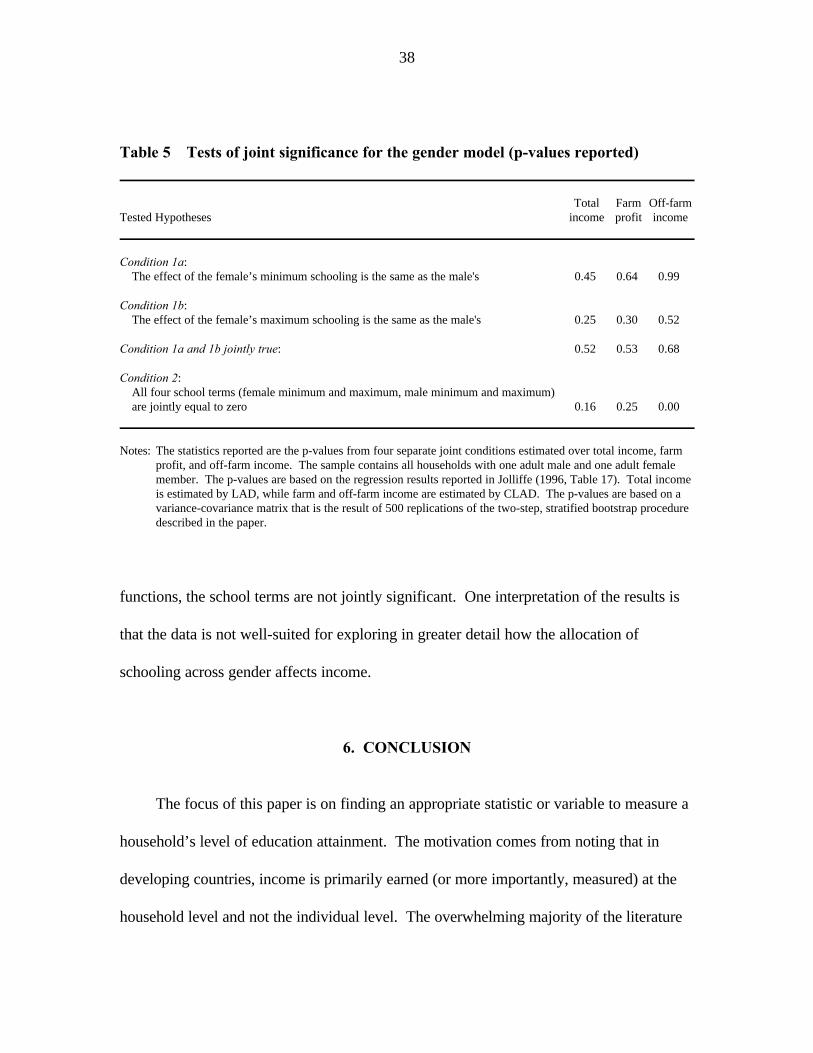
Table 5—Tests of joint significance for the gender model (p-values reported)

Total Farm Off-farmTested Hypotheses income profit income

Condition 1a:The effect of the female’s minimum schooling is the same as the male's 0.45 0.64 0.99

Condition 1b:The effect of the female’s maximum schooling is the same as the male's 0.25 0.30 0.52

Condition 1a and 1b jointly true: 0.52 0.53 0.68

Condition 2:All four school terms (female minimum and maximum, male minimum and maximum)are jointly equal to zero 0.16 0.25 0.00

Notes: The statistics reported are the p-values from four separate joint conditions estimated over total income, farmprofit, and off-farm income. The sample contains all households with one adult male and one adult femalemember. The p-values are based on the regression results reported in Jolliffe (1996, Table 17). Total incomeis estimated by LAD, while farm and off-farm income are estimated by CLAD. The p-values are based on avariance-covariance matrix that is the result of 500 replications of the two-step, stratified bootstrap proceduredescribed in the paper.

functions, the school terms are not jointly significant. One interpretation of the results is

that the data is not well-suited for exploring in greater detail how the allocation of

schooling across gender affects income.

6. CONCLUSION

The focus of this paper is on finding an appropriate statistic or variable to measure a

household’s level of education attainment. The motivation comes from noting that in

developing countries, income is primarily earned (or more importantly, measured) at the

household level and not the individual level. The overwhelming majority of the literature

39

The rejection of both of these models is robust to whether total income, farm profit, or off-farm52

income is estimated, using either the full sample of all households, or the sample of households with two ormore adults, or the sample with three or more adults.

No attempt is made in this paper to explain why the average level of schooling is important for farm53

and off-farm income, while the maximum level of schooling is important for total income. These results arecertainly consistent with the hypothesis that the intrahousehold allocation of education affects householdincome in a complex way. Attempting to produce a richer explanation of how the intrahousehold allocationaffects household income is an example of the type of future research this project points toward.

assumes that the education attainment of the head of household measures the entire

household’s level of education attainment. On the basis of only the basic descriptive

statistics presented in this paper, this assumption appears dubious.

This paper presents further evidence against using the head of household by testing

three competing models of school attainment against each other and against the head of

household model. The most unambiguous result in this paper is the robust rejection of the

weakest link and head of household model. While the estimation results reject using52

either the minimum level or the head’s level of education to measure household school

attainment, they show support for using the maximum level of school attainment when

estimating total household income. The data also show support for using the average

level of schooling when estimating farm and off-farm income.53

This paper also asserts that it is important to examine estimates that are robust to

violations of normality. Many data sets, particularly data resulting from household

surveys in developing countries, are fraught with numerous outliers and other violations of

normality. The GLSS data are shown to be no exception to this statement. Similarly, the

40

large majority of nationally representative household data sets is based on complex sample

designs, which need to be incorporated into the estimation strategy.

The brief summary in Table 4 shows that the differences between OLS and LAD

estimates are large. This supports the claim that nonnormalities in general, or outliers in

particular, are important to the results and support using estimators like LAD that are

robust to these types of violations of normality. Table 4 also shows that the effect of

correcting estimated LAD standard errors for violations of the iid assumption is also large.

This paper attempts to explore a richer model of household school attainment that

incorporates the possibility that how schooling is distributed across the male and female

members may also be an important determinant of income. The GLSS data do not

support the hypothesis that it is important to capture the gender differences in school

attainment when estimating household income. This rejection, though, is weak, and

primarily suggests that the hypothesis is not well tested with the GLSS data.

The attempt to test whether schooling affects household income differently if held by

a male or female is a good example of the type of research this paper points toward. This

paper focuses on finding a unidimensional statistic to measure household school

attainment, which is a complex, multidimensional characteristic. While the paper shows

that the maximum and the average level of schooling are both better measures of

household school attainment than the minimum or household head’s, these measures are

still somewhat naive and restrictive. An area for future research, then, is to explore in

more detail how the allocation of education across different household members of

41

different ages or genders and across individuals engaged in different activities, affects

household income.

APPENDIX

Table 6—Descriptive statistics

StandardVariable Observations Mean Deviation Minimum Maximum

IncomeLog: Total household income 1,547 11.02 3.137 0 18.76Log: Restricted farm profit 1,547 8.04 5.160 0 14.15Log: Off-farm income 1,547 7.29 5.379 0 18.76

Schoolinga

Household minimum level of schooling 1,547 3.80 4.711 0 20Household median level of schooling 1,547 5.55 4.763 0 21.5Household maximum level of schooling 1,547 7.40 5.247 0 23Household head: Schooling 1,547 5.63 5.566 0 23Household average: Years of schooling 1,547 5.58 4.516 0 21.5Household minimum male schooling 921 6.16 5.357 0 23Household minimum female schooling 921 3.39 4.528 0 20Household maximum male schooling 921 7.62 5.381 0 23Household maximum female schooling 921 4.94 4.958 0 20

Farm incomeLog (acres of land farmed) 1,547 1.90 1.906 0 6.55Household average: Log of farm experience 1,547 1.70 1.231 0 4.19Cluster/Zone average: Day farm wage 1,547 3.44 1.120 0 6Region average: Ln(price fertilizer) 1,547 7.57 0.245 7.05 7.93Region average: Ln(price insecticide) 1,547 7.11 0.508 6.19 7.85Region average: Price of maize 1,547 51.56 24.264 20 157.5Region average: Price of okra 1,547 6.75 3.490 2 32Region average: Price of cassava 1,547 11.28 8.678 0.07 40Region average: Price of pepper 1,547 29.45 9.754 6 58.88

Off-farm incomeLog: Business assets 1,547 3.72 4.384 0 19.60Household maximum: ln(off-farm experience) 1,547 1.58 1.187 0 4.511Area average: Off-farm wage, type 1 1,547 0.350 0.111 0.082 0.454Area average: Off-farm wage, type 2 1,547 0.470 0.148 0.204 0.654Area average: Off-farm wage, type 3 1,547 0.751 0.243 0.388 1.093Area average: Off-farm wage, type 4 1,547 0.833 0.321 0.385 1.532Area average: Off-farm wage, type 5 1,547 2.165 1.061 0.990 3.883

Household characteristicsNumber of males: 15-24 years old 1,547 0.387 0.692 0 5Number of males: 25-34 years old 1,547 0.237 0.443 0 3Number of males: 35-44 years old 1,547 0.173 0.379 0 1Number of males: 45-55 years old 1,547 0.125 0.331 0 1Number of females: 15-24 years old 1,547 0.388 0.642 0 5Number of females: 25-34 years old 1,547 0.310 0.498 0 3Number of females: 35-44 years old 1,547 0.176 0.396 0 2Number of females: 45-55 years old 1,547 0.157 0.385 0 3

The sample size for the most (and least) educated male and female in the household is 921. For the example ona

gender differences, only those households with at least one adult male and female are included.

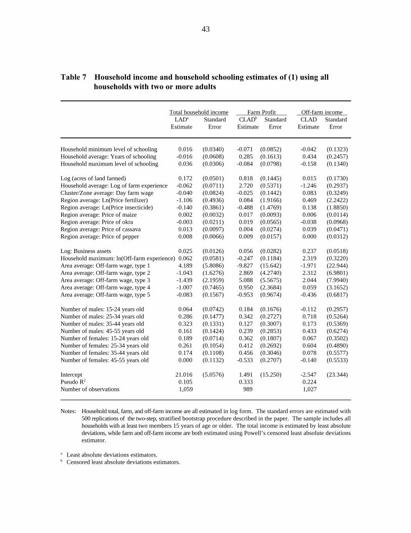
43

Table 7—Household income and household schooling estimates of (1) using allhouseholds with two or more adults

Total household income Farm Profit Off-farm income LAD Standard CLAD Standard CLAD Standarda b

Estimate Error Estimate Error Estimate Error

Household minimum level of schooling 0.016 (0.0340) -0.071 (0.0852) -0.042 (0.1323)Household average: Years of schooling -0.016 (0.0608) 0.285 (0.1613) 0.434 (0.2457)Household maximum level of schooling 0.036 (0.0306) -0.084 (0.0798) -0.158 (0.1340)

Log (acres of land farmed) 0.172 (0.0501) 0.818 (0.1445) 0.015 (0.1730)Household average: Log of farm experience -0.062 (0.0711) 2.720 (0.5371) -1.246 (0.2937)Cluster/Zone average: Day farm wage -0.040 (0.0824) -0.025 (0.1442) 0.083 (0.3249)Region average: Ln(Price fertilizer) -1.106 (0.4936) 0.084 (1.9166) 0.469 (2.2422)Region average: Ln(Price insecticide) -0.140 (0.3861) -0.488 (1.4769) 0.138 (1.8850)Region average: Price of maize 0.002 (0.0032) 0.017 (0.0093) 0.006 (0.0114)Region average: Price of okra -0.003 (0.0211) 0.019 (0.0565) -0.038 (0.0968)Region average: Price of cassava 0.013 (0.0097) 0.004 (0.0274) 0.039 (0.0471)Region average: Price of pepper 0.008 (0.0066) 0.009 (0.0157) 0.000 (0.0312)

Log: Business assets 0.025 (0.0126) 0.056 (0.0282) 0.237 (0.0518)Household maximum: ln(Off-farm experience) 0.062 (0.0581) -0.247 (0.1184) 2.319 (0.3220)Area average: Off-farm wage, type 1 4.189 (5.8086) -9.827 (15.642) -1.971 (22.944)Area average: Off-farm wage, type 2 -1.043 (1.6276) 2.869 (4.2740) 2.312 (6.9801)Area average: Off-farm wage, type 3 -1.439 (2.1959) 5.088 (5.5675) 2.044 (7.9940)Area average: Off-farm wage, type 4 -1.007 (0.7465) 0.950 (2.3684) 0.059 (3.1652)Area average: Off-farm wage, type 5 -0.083 (0.1567) -0.953 (0.9674) -0.436 (0.6817)

Number of males: 15-24 years old 0.064 (0.0742) 0.184 (0.1676) -0.112 (0.2957)Number of males: 25-34 years old 0.286 (0.1477) 0.342 (0.2727) 0.718 (0.5264)Number of males: 35-44 years old 0.323 (0.1331) 0.127 (0.3007) 0.173 (0.5369)Number of males: 45-55 years old 0.161 (0.1424) 0.239 (0.2853) 0.433 (0.6274)Number of females: 15-24 years old 0.189 (0.0714) 0.362 (0.1807) 0.067 (0.3502)Number of females: 25-34 years old 0.261 (0.1054) 0.412 (0.2692) 0.604 (0.4890)Number of females: 35-44 years old 0.174 (0.1108) 0.456 (0.3046) 0.078 (0.5577)Number of females: 45-55 years old 0.000 (0.1132) -0.533 (0.2707) -0.140 (0.5533)

Intercept 21.016 (5.0576) 1.491 (15.250) -2.547 (23.344)Pseudo R 0.105 0.333 0.2242

Number of observations 1,059 989 1,027

Notes: Household total, farm, and off-farm income are all estimated in log form. The standard errors are estimated with500 replications of the two-step, stratified bootstrap procedure described in the paper. The sample includes allhouseholds with at least two members 15 years of age or older. The total income is estimated by least absolutedeviations, while farm and off-farm income are both estimated using Powell’s censored least absolute deviationsestimator.

Least absolute deviations estimators.a

Censored least absolute deviations estimators.b

44

Table 8—Total household income and household schooling: Comparison of householdhead’s schooling, maximum, and average schooling

LAD Standard LAD Standard LAD Standarda

Estimate Error Estimate Error Estimate Error

Household head: Schooling 0.037 (0.0114)Household maximum level of schooling 0.047 (0.0125)Household average level of schooling 0.052 (0.0140)

Log(acres of land farmed) 0.148 (0.0416) 0.132 (0.0416) 0.150 (0.0449)Household average: log of farm experience 0.101 (0.0659) 0.080 (0.0646) 0.095 (0.0657)Cluster/Zone average: Day farm wage -0.032 (0.0778) -0.078 (0.0896) -0.040 (0.0818)Region average: Ln(price fertilizer) -1.219 (0.5598) -1.257 (0.5159) -1.135 (0.4972)Region average: Ln(price insecticide) -0.049 (0.3917) -0.158 (0.3790) -0.125 (0.3637)Region average: Price of maize 0.004 (0.0031) 0.004 (0.0031) 0.004 (0.0030)Region average: Price of okra -0.002 (0.0237) 0.004 (0.0264) 0.002 (0.0246)Region average: Price of cassava 0.017 (0.0102) 0.017 (0.0097) 0.017 (0.0094)Region average: Price of pepper 0.006 (0.0067) 0.007 (0.0072) 0.007 (0.0076)

Log: Business assets 0.025 (0.0132) 0.023 (0.0136) 0.023 (0.0121)Household maximum: ln(Off-farm experience) 0.166 (0.0539) 0.153 (0.0535) 0.163 (0.0515)Area average: Off-farm wage, type 1 5.383 (6.4705) 7.175 (6.6618) 6.488 (6.1948)Area average: Off-farm wage, type 2 -1.072 (1.7531) -1.701 (1.8695) -1.566 (1.7599)Area average: Off-farm wage, type 3 -1.696 (2.4473) -2.414 (2.5377) -2.178 (2.3629)Area average: Off-farm wage, type 4 -1.280 (0.8637) -1.396 (0.8583) -1.336 (0.7861)Area average: Off-farm wage, type 5 -0.175 (0.1639) -0.152 (0.1544) -0.136 (0.1447)

Number of males: 15-24 years old 0.135 (0.0699) 0.076 (0.0661) 0.101 (0.0678)Number of males: 25-34 years old 0.446 (0.1410) 0.442 (0.1315) 0.447 (0.1434)Number of males: 35-44 years old 0.442 (0.1302) 0.465 (0.1284) 0.494 (0.1289)Number of males: 45-55 years old 0.256 (0.1530) 0.303 (0.1494) 0.266 (0.1559)Number of females: 15-24 years old 0.344 (0.0735) 0.263 (0.0727) 0.321 (0.0744)Number of females: 25-34 years old 0.359 (0.1081) 0.307 (0.1149) 0.322 (0.1019)Number of females: 35-44 years old 0.234 (0.1275) 0.207 (0.1284) 0.281 (0.1312)Number of females: 45-55 years old 0.012 (0.1327) -0.019 (0.1343) 0.003 (0.1294)

Intercept 20.604 (5.2683) 22.018 (5.1657) 20.606 (4.9686)

Pseudo R 0.118 0.117 0.1192

Number of observations 1,547 1,547 1,547

Notes: Household total income is estimated in log form. The standard errors are estimated with 500 replications of thetwo-step, stratified bootstrap procedure described in the paper. The sample includes all households with at leastone member 15 years of age or older.

Least absolute deviations estimators.a

REFERENCES

Arabmazar, A., and P. Schmidt. 1981. Further evidence on the robustness of the Tobit

estimator to heteroscedasticity. Journal of Econometrics 17 (2): 253–258.

Breusch, T. S., and A. R. Pagan. 1979. A simple test for heteroscedasticity and random

coefficient variation. Review of Economic Studies 47 (5): 1287–1294.

Buchinsky, M. 1991. Methodological issues in quantile regression. In The theory and

practice of quantile regression. Chapter 1. Ph.D. diss., Harvard University,

Cambridge, Mass., U.S.A.

Buchinsky, M. 1994. Changes in the U.S. wage structure 1963-1987: Application of

quantile regression. Econometrica 62 (2): 405–459.

Fane, G. 1975. Education and the managerial efficiency of farmers. Review of

Economics and Statistics 57 (4): 452–461.

Ghana Statistical Service. 1991a. Statistical News Letter. No. A11/91. Accra, Ghana.

Ghana Statistical Service. 1991b. Quarterly Digest of Statistics 9 (4). Accra, Ghana.

Glewwe, P., and K. A. Twum-Baah. 1991. The distribution of welfare in Ghana in

1987-1988. Living Standards Measurement Study Working Paper 75. Washington,

D.C.: World Bank.

Grigg, D. 1991. The transformation of agriculture in the West. Cambridge, Mass.,

U.S.A.: Basil Blackwell Press.

Howe, S., and J. Lanjouw-Olson. 1995. Making poverty comparisons taking into

account survey design: How and why. World Bank, Washington, D.C., and Yale

University, New Haven, Conn., U.S.A. Photocopied.

46

Huffman, W. E. 1974. Decisionmaking: The role of education. American Journal of

Agricultural Economics 56 (1): 85–97.

Jamison, D. T., and L. J. Lau. 1982. Farmer education and farm efficiency.

Washington, D.C.: World Bank.

Jamison, D. T., and P. R. Moock. 1984. Farmer education and farm efficiency in Nepal:

The role of schooling, extension services, and cognitive skills. World Development

12 (1): 67–86.

Jolliffe, D. 1996. Cognitive skills, schooling, and household income: An econometric

analysis using data from Ghana. Ph.D. diss., Princeton University, Princeton, N.J.,

U.S.A.

Koenker, R., and G. Bassett. 1978. Regression quantiles. Econometrica 46 (1): 33–50.

Lin, J. Y. 1991. Education and innovation adoption: Evidence from hybrid Rice in

China. American Journal of Agricultural Economics 73 (3): 713–723.

Pagan, A., and F. Vella. 1989. Diagnostic tests for models based on individual data: A

survey. Journal of Applied Econometrics 4 (December) (Supplement): S29–S59.

Powell, J. L. 1984. Least absolute deviations estimation for the censored regression

model. Journal of Econometrics 25 (3): 303–325.

Psacharopoulos, G. 1981. Returns to education: An updated international comparison.

Comparative Education 17 (3): 321–341.

Psacharopoulos, G. 1985. Returns to education: A further international update and

implications. Journal of Human Resources 20 (2): 583–604.

47

Psacharopoulos, G. 1994. Returns to investment in education: A global update. World

Development 22 (9): 1325–1343.

Rogers, W. 1993. Calculation of quantile regression standard errors. Stata Technical

Bulletin STB-13: 18–19.

Scott, A. J., and D. Holt. 1982. The effect of two-stage sampling on ordinary least

squares methods. Journal of American Statistical Association 77 (380): 848–854.

Scott, C., and B. Amenuvegbe. 1989. Sample designs for the Living Standards surveys

in Ghana and Mauritania. Living Standards Measurement Study Working Paper

49. Washington, D.C.: World Bank.

Shapiro, S., and R. Francia. 1972. An approximate analysis of variance test for normality.

Journal of the American Statistical Association 67 (337): 215–216.

Vijverberg, W. 1987. Non-normality as distributional misspecification in single-equation

limited dependent variable models. Oxford Bulletin of Economics and Statistics 49

(4): 417–430.

Vijverberg, W. 1991a. Schooling, skills and income from nonfarm self-employment in

Ghana. University of Texas at Dallas, Dallas, Texas, U.S.A. Photocopied.

Vijverberg, W. 1991b. Measuring income from family enterprises with household

surveys. Living Standards Measurement Study Working Paper 84. Washington,

D.C.: World Bank.

48

World Bank. 1995. World development report 1995: Workers in an integrating world.

Washington, D.C.: Oxford University Press.

Wu, C. C. 1977. Education in farm production: The case of Taiwan. American Journal

of Agricultural Economics 59 (4): 699–709.