SERC DISCUSSION PAPER 89

On the Relative Importance ofAgglomeration Economies in theLocation of FDI Across British RegionsJonathan Jones (SERC, Newcastle University Business School)Colin Wren (SERC, Newcastle University Business School)

August 2011

This work is part of the research programme of the independent UK Spatial

Economics Research Centre funded by the Economic and Social Research Council

(ESRC), Department for Business, Innovation and Skills (BIS), the Department for

Communities and Local Government (CLG), and the Welsh Assembly Government.

The support of the funders is acknowledged. The views expressed are those of the

authors and do not represent the views of the funders.

© J. Jones and C. Wren, submitted 2011

On the Relative Importance of Agglomeration Economies

in the Location of FDI across British Regions

Jonathan Jones* and Colin Wren**

August 2011

* SERC, Newcastle University Business School

** SERC, Economics, Newcastle University Business School

Acknowledgements

The authors gratefully acknowledge financial support from the ESRC Spatial Economic

Research Centre (http://www.spatialeconomics.ac.uk). Earlier versions of this paper were

presented at the British and Irish Section of the Regional Science Association International,

Glasgow, August 2010, and the INFER conference, Orléans, France, March 2011. The

authors are grateful for comments from participants at these events.

Abstract

The paper examines the relative importance for industrial location of production linkages and

knowledge spillovers, distinguishing between intermediate and non-intermediate goods that

are backwards or forwards in nature. A novel approach is used to construct proxies for non-

intermediate goods at a sub-national industry level based on an Input-Output transaction

table. Taking data on location decisions by foreign-owned plants across British regions over

1985-2007, the paper finds support for the new economic geography explanation of location

based on linkages over that due to spillovers. However, the importance of intermediate and

non-intermediate linkages differs between manufacturing and service industries.

Keywords: Industrial location; agglomeration economies; intermediate goods; FDI

JEL Classifications: H3, O2, L2, R3

2

1 Introduction

Agglomeration economies reflect proximity and are an important explanation for industrial

location. They have antecedents in the work of Marshall (1920), and feature prominently in

the recent theories of location, including the intermediate inputs (Venables, 1996) and labour

mobility (Krugman, 1991) of the new economic geography and the knowledge spillovers of

the new growth theory (Griliches, 1992). However, while there is a good supply of theories,

there is much less evidence on the relative importance of these explanations, which Ellison et

al (2010) characterize as “the cost of moving goods, people, and ideas” (p. 1195). It is partly

because research on agglomeration economies tends to be partial, so that production linkages

are often ignored in the literature on knowledge spillovers (e.g. Rosenthal and Strange, 2004)

and conversely (e.g. Amiti and Javorcik, 2008).1 Further, there is the difficulty of adequately

measuring all production linkages at the sub-national industry level, which include backward

and forward effects in both intermediate and non-intermediate goods markets.

This paper examines the relative strength of the different agglomeration economies on

industrial location, adopting a novel approach to measure the strength of the non-intermediate

goods at the sub-national industry level. This is based on an Input-Output transaction table,

which not only incorporates the „core Input-Output table‟ that shows the exchange of goods

and services between industries, but records the flows of goods and services to or from agents

that are outside of the industrial sector, e.g. labour services and final household demand (see

Armstrong and Taylor, 2000). The approach is advantageous, as in an accounting sense it

permits all possible non-intermediate and intermediate goods to be included, and which are

measured on a comparable basis. In this paper two forward non-intermediate goods terms are

included, for final domestic demand and exports, and two backward non-intermediate terms

for the gross value added of labour services and residual surplus. Terms are also included for

the backward and forward intermediate goods and for knowledge spillovers.

The investigation utilises data on about 13,000 investments by foreign-owned plants

across the regions of Great Britain over the period 1985-2007. The data relate to flows rather

than stocks (i.e. the location decision), while foreign direct investment (FDI) is highly mobile

across geographic space. The data are known for both manufacturing and service industries.

The linkage terms are constructed from the UK Supply and Use Table, which is a transaction

1 Ellison et al (2010) use input-output and other tables to measure the strength of three Marshallian economies

between industry pairs. In principle, this approach could be extended to include other sources of agglomeration

economy, but it has strong data requirements, while it is regressed for a single cross-section, which as Ellison et

al acknowledge, raises issues about the role of natural advantages.

3

table that is available at the national level only. This restricts the analysis to NUTS 1 regions,

although offering a good trade-off between the geographical reach of production linkages and

knowledge spillovers. Research finds that spillovers can extend over large areas (see Döring

and Schnellenbach, 2006; Baldwin et al, 2008), while Lamorgese and Ottaviano (2002) argue

that if anything pecuniary effects occur over relatively greater distances.2

The paper finds significant effects for each kind of agglomeration economy, which is

sensitive to the inclusion of all such terms. Overall, when calculated on a comparable basis

as elasticities, the production linkages are more important for location than are knowledge

spillovers, which supports the new economic geography over the new growth theory. In their

relative effect the estimates differ between sectors, which indicates that this is a consideration

when discriminating between competing explanations. Thus, backward intermediate goods

markets are important for manufacturing and forward intermediate goods are more important

for services, while the opposite tends to be the case for non-intermediate goods (e.g. labour is

relatively more important for services and exports less important). In the case of knowledge

spillovers there are significant differences between industries, which indicate differences in

the transferability of knowledge between these sectors. Intra-industry flows have a relatively

greater effect on manufacturing location but inter-industry flows more so for services.

In the next section, the literature is reviewed and the measurement of the intermediate

and non-intermediate goods terms is considered. Section 3 sets out the empirical model and

section 4 describes the data. The results are presented in section 5 and section 6 concludes.

2 Intermediate and Non-Intermediate Linkages

Agglomeration economies are an important factor in FDI location, but in the literature these

were initially measured at the aggregate level, as either the employment level or the number

of plants in an area (e.g. Coughlin et al, 1991; Wheeler and Mody, 1992; Woodward, 1992),

and only occasionally at the industry level (Carlton, 1983). Later studies distinguish between

domestic and foreign firms, such as Head et al (1995), and a consistent finding is that foreign

2 Rosenthal and Strange (2001) and Henderson (2003) find that spillovers attenuate rapidly with distance, but

Beenstock and Felsenstein (2010) argue that there is no intrinsic reason why these should be restricted to a local

level. Jaffe et al (1993) and Audretsch and Feldman (1996) find evidence for knowledge spillovers at the level

of US states, and others at even greater distances. Significant spatial lag effects are found below for linkages

and spillovers, indicating that these flow between the NUTS 1 regions. The use of NUTS 1 regions means that

there are is a choice for each investment across ten regions only, but the data are available for a long time period,

over which the agglomeration terms and other controls vary greatly, offering a good test of the approach.

4

plants exert a stronger influence on FDI location than do domestic plants, whether or not the

FDI originates from the same source country (e.g. Crozet et al, 2004; Hilber and Voicu, 2007;

Devereux et al, 2007; and Basile et al, 2008). This is generally attributed to agglomeration

economies, although it could pick-up an unobserved location effect, such as demand or even

an information asymmetry on the host economy (Procher, 2009; Mariotti et al, 2010).

When consideration is given to the nature of an agglomeration economy affecting FDI

location, early studies also do not impose any formal linkage structure on the data (e.g. Head

and Mayer, 2004). This is achieved by the use of input-output tables to examine backward or

forward intermediate effects (Javorcik, 2004), although research has generally focused on just

one of these (e.g. Milner et al, 2006, on backward linkages for Japanese FDI in Thailand and

Bekes, 2006, on forward FDI linkages in Hungary). In the relatively small number of studies

that consider both kinds of effect there are omissions that can give rise to identification issues.

Thus, Amiti and Javorcik (2008) consider input-output linkages and omit externalities, but

the input-output tables may also used to examine the channels through which the spillovers

occur (e.g. Driffield et al, 2004; Javorcik and Spartareanu, 2009; Mariotti et al, 2010). Du et

al (2008) and Debaere et al (2010) include terms for externalities, but do not allow for the

inter-industry economies that can arise from industrial diversity. Finally, even when a full set

of terms is included, such as in Lee et al (2008), the differences between the intermediate and

non-intermediate goods are not analysed, so that the relative importance of the different kinds

of agglomeration economy remains to be fully explored in the literature.

2.1 Measurement of the Linkage Terms

Expressions for the intermediate and non-intermediate linkage terms are now derived. These

are based on the Input-Output transaction table that includes all inputs and outputs, such that

total output is equal to total inputs for each industry. Initially, the intermediate goods term is

derived based on the Input-Output (I/O) core table, i.e. the processing sector for the domestic

industry (see Armstrong and Taylor, 2000). The purpose of this is to show that this can give

biased estimates, even though linkage terms based on this or similar are used in the literature.

The linkage terms that are adopted in this paper are then presented. Each is for the backward

effect, while Appendix A gives the expressions for the corresponding forward terms.

Suppose there are K industries and that firms in each industry are homogeneous. Let

ql be the total value of output of industry l {1, 2, …, K}, and suppose that this industry uses

5

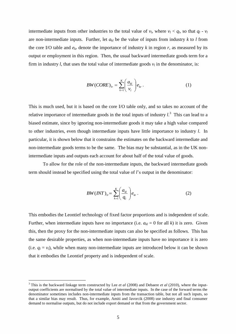
intermediate inputs from other industries to the total value of vl, where vl < ql, so that ql - vl

are non-intermediate inputs. Further, let akl be the value of inputs from industry k to l from

the core I/O table and ekr denote the importance of industry k in region r, as measured by its

output or employment in this region. Then, the usual backward intermediate goods term for a

firm in industry l, that uses the total value of intermediate goods vl in the denominator, is:

kr

K

k l

kllr e

v

aCOREBW

1

)( . (1)

This is much used, but it is based on the core I/O table only, and so takes no account of the

relative importance of intermediate goods in the total inputs of industry l.3 This can lead to a

biased estimate, since by ignoring non-intermediate goods it may take a high value compared

to other industries, even though intermediate inputs have little importance to industry l. In

particular, it is shown below that it constrains the estimates on the backward intermediate and

non-intermediate goods terms to be the same. The bias may be substantial, as in the UK non-

intermediate inputs and outputs each account for about half of the total value of goods.

To allow for the role of the non-intermediate inputs, the backward intermediate goods

term should instead be specified using the total value of l‟s output in the denominator:

kr

K

k l

kllr e

q

aINTBW

1

)( . (2)

This embodies the Leontief technology of fixed factor proportions and is independent of scale.

Further, when intermediate inputs have no importance (i.e. akl = 0 for all k) it is zero. Given

this, then the proxy for the non-intermediate inputs can also be specified as follows. This has

the same desirable properties, as when non-intermediate inputs have no importance it is zero

(i.e. ql = vl), while when many non-intermediate inputs are introduced below it can be shown

that it embodies the Leontief property and is independent of scale.

3 This is the backward linkage term constructed by Lee et al (2008) and Debaere et al (2010), where the input-

output coefficients are normalised by the total value of intermediate inputs. In the case of the forward terms the

denominator sometimes includes non-intermediate inputs from the transaction table, but not all such inputs, so

that a similar bias may result. Thus, for example, Amiti and Javorcik (2008) use industry and final consumer

demand to normalise outputs, but do not include export demand or that from the government sector.

6

kr

K

k l

kl

l

llr e

q

a

v

qINTNONBW

1

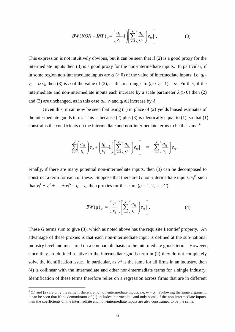
1)( . (3)

This expression is not intuitively obvious, but it can be seen that if (2) is a good proxy for the

intermediate inputs then (3) is a good proxy for the non-intermediate inputs. In particular, if

in some region non-intermediate inputs are (> 0) of the value of intermediate inputs, i.e. ql -

vl, = vl, then (3) is of the value of (2), as this rearranges to (ql / vl - 1) = . Further, if the

intermediate and non-intermediate inputs each increase by a scale parameter then (2)

and (3) are unchanged, as in this case akl, vl and ql all increase by .

Given this, it can now be seen that using (1) in place of (2) yields biased estimates of

the intermediate goods term. This is because (2) plus (3) is identically equal to (1), so that (1)

constrains the coefficients on the intermediate and non-intermediate terms to be the same:4

kr

K

k l

klkr

K

k l

kl

l

lkr

K

k l

kl ev

ae

q

a

v

qe

q

a

111

1 .

Finally, if there are many potential non-intermediate inputs, then (3) can be decomposed to

construct a term for each of these. Suppose that there are G non-intermediate inputs, vlg, such

that vl1 + vl

2 + … + vl

G = ql - vl, then proxies for these are (g = 1, 2, …, G):

kr

K

k l

kl

l

g

llr e

q

a

v

vgBW

1

)( . (4)

These G terms sum to give (3), which as noted above has the requisite Leontief property. An

advantage of these proxies is that each non-intermediate input is defined at the sub-national

industry level and measured on a comparable basis to the intermediate goods term. However,

since they are defined relative to the intermediate goods term in (2) they do not completely

solve the identification issue. In particular, as vlg is the same for all firms in an industry, then

(4) is collinear with the intermediate and other non-intermediate terms for a single industry.

Identification of these terms therefore relies on a regression across firms that are in different

4 (1) and (2) are only the same if there are no non-intermediate inputs, i.e. vl = ql. Following the same argument,

it can be seen that if the denominator of (1) includes intermediate and only some of the non-intermediate inputs,

then the coefficients on the intermediate and non-intermediate inputs are also constrained to be the same.

7

industries, so that there must be a reasonable number of these industries.

3 Empirical Model of Location Choice

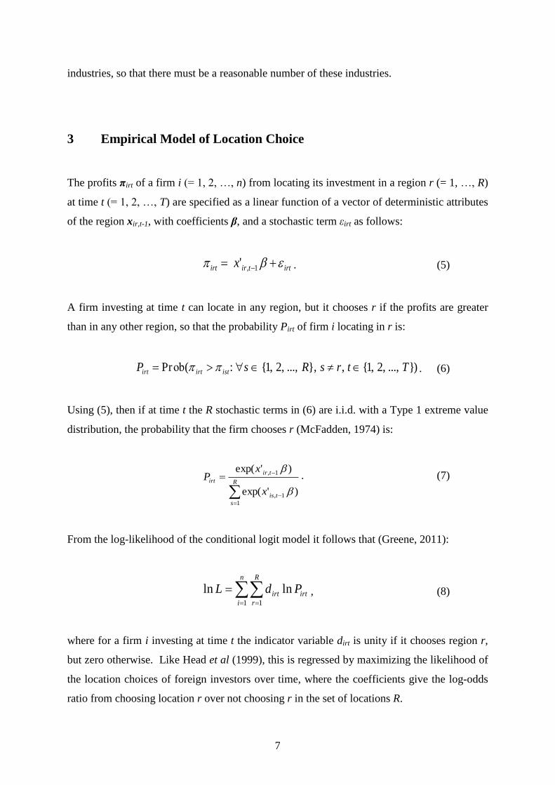
The profits πirt of a firm i (= 1, 2, …, n) from locating its investment in a region r (= 1, …, R)

at time t (= 1, 2, …, T) are specified as a linear function of a vector of deterministic attributes

of the region xir,t-1, with coefficients β, and a stochastic term εirt as follows:

irttirirt x 1,' . (5)

A firm investing at time t can locate in any region, but it chooses r if the profits are greater

than in any other region, so that the probability Pirt of firm i locating in r is:

)}...,,2,1{,},...,,2,1{:(Pr TtrsRsP istirtirt ob . (6)

Using (5), then if at time t the R stochastic terms in (6) are i.i.d. with a Type 1 extreme value

distribution, the probability that the firm chooses r (McFadden, 1974) is:

R

s

tis

tir

irt

x

xP

1

1,

1,

)'exp(

)'exp(

. (7)

From the log-likelihood of the conditional logit model it follows that (Greene, 2011):

n

i

R

r

irtirt PdL1 1

lnln , (8)

where for a firm i investing at time t the indicator variable dirt is unity if it chooses region r,

but zero otherwise. Like Head et al (1999), this is regressed by maximizing the likelihood of

the location choices of foreign investors over time, where the coefficients give the log-odds

ratio from choosing location r over not choosing r in the set of locations R.

8

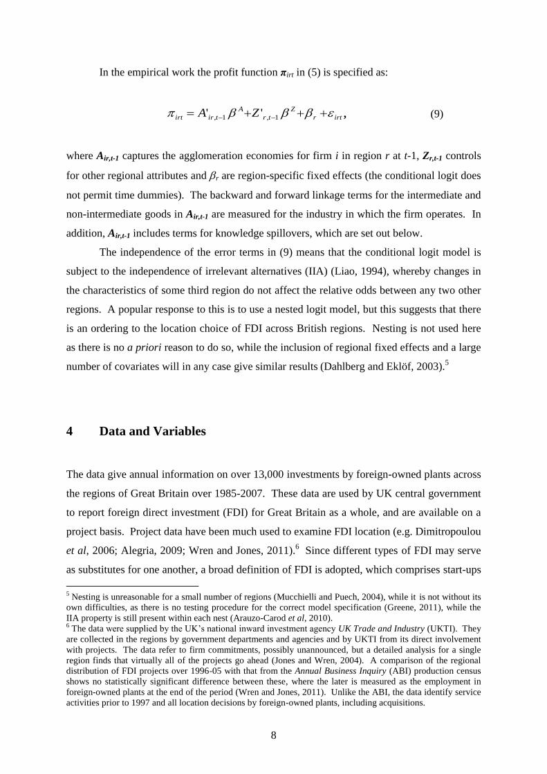
In the empirical work the profit function πirt in (5) is specified as:

irtr

Z

tr

A

tirirt ZA 1,1, '' , (9)

where Air,t-1 captures the agglomeration economies for firm i in region r at t-1, Zr,t-1 controls

for other regional attributes and r are region-specific fixed effects (the conditional logit does

not permit time dummies). The backward and forward linkage terms for the intermediate and

non-intermediate goods in Air,t-1 are measured for the industry in which the firm operates. In

addition, Air,t-1 includes terms for knowledge spillovers, which are set out below.

The independence of the error terms in (9) means that the conditional logit model is

subject to the independence of irrelevant alternatives (IIA) (Liao, 1994), whereby changes in

the characteristics of some third region do not affect the relative odds between any two other

regions. A popular response to this is to use a nested logit model, but this suggests that there

is an ordering to the location choice of FDI across British regions. Nesting is not used here

as there is no a priori reason to do so, while the inclusion of regional fixed effects and a large

number of covariates will in any case give similar results (Dahlberg and Eklöf, 2003).5

4 Data and Variables

The data give annual information on over 13,000 investments by foreign-owned plants across

the regions of Great Britain over 1985-2007. These data are used by UK central government

to report foreign direct investment (FDI) for Great Britain as a whole, and are available on a

project basis. Project data have been much used to examine FDI location (e.g. Dimitropoulou

et al, 2006; Alegria, 2009; Wren and Jones, 2011).6 Since different types of FDI may serve

as substitutes for one another, a broad definition of FDI is adopted, which comprises start-ups

5 Nesting is unreasonable for a small number of regions (Mucchielli and Puech, 2004), while it is not without its

own difficulties, as there is no testing procedure for the correct model specification (Greene, 2011), while the

IIA property is still present within each nest (Arauzo-Carod et al, 2010). 6 The data were supplied by the UK‟s national inward investment agency UK Trade and Industry (UKTI). They

are collected in the regions by government departments and agencies and by UKTI from its direct involvement

with projects. The data refer to firm commitments, possibly unannounced, but a detailed analysis for a single

region finds that virtually all of the projects go ahead (Jones and Wren, 2004). A comparison of the regional

distribution of FDI projects over 1996-05 with that from the Annual Business Inquiry (ABI) production census

shows no statistically significant difference between these, where the later is measured as the employment in

foreign-owned plants at the end of the period (Wren and Jones, 2011). Unlike the ABI, the data identify service

activities prior to 1997 and all location decisions by foreign-owned plants, including acquisitions.

9

(„greenfield‟ investments), acquisitions and re-investments, where each of these is potentially

mobile across regions.7 Re-investments involve a substantial upgrading to an existing plant,

e.g. a new production line, for which further details are given in Wren and Jones (2009).

The areas are the Government Office Regions for Great Britain, where London is

included in the South East region, giving ten regions (R = 10).8 Brand et al (2000) find that

the regions build-up FDI in distinct activities, which offers prima facie evidence for the

existence of agglomeration economies at this level. Input-output tables are not produced at

the sub-national level, but as noted above the regions are sufficiently large in scale to offer a

good trade-off between the likely spatial reach of linkages and spillovers. The FDI data are

available at the 3-digit industry level, but the UK input-output tables report the coefficients

for 123 industry groups that range from aggregates of 2-digit industries to single 4-digit

industries. These map to the 97 divisions of the NACE industrial classification (ONS, 2006),

but as some industries receive little or no FDI then 46 broadly homogeneous industries are

formed through aggregation (K = 46). These are given in Appendix B, which shows that 23

industries are in manufacturing and 19 in services.9 They are based on 2-digit industries,

although disaggregated to identify several activities where FDI is particularly strong.

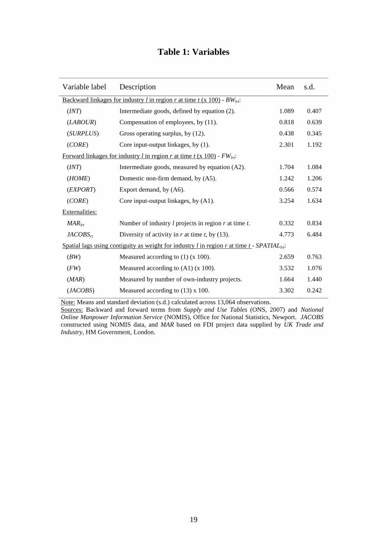
The measurement of the variables is now considered, which begins with those for the

agglomeration terms in Airt in (9). The variables and their labels are given in table 1.

4.1 Intermediate goods

The intermediate goods terms are constructed from the input-output coefficients of the UK

Supply and Use Table. For years prior to 1995 this table is produced at 5-year intervals using

a different industrial classification, so that a single table is used for 1995 (ONS, 2007), which

is similar to the practice adopted elsewhere.10

The input-output coefficients akl are essentially

7 The data include a small numbers of joint ventures and mergers. Start-ups and re-investments each account for

about 40% of the total number of projects. 8 These are the Eurostat NUTS 1 regions. The London Government Office Region is drawn tightly around the

urban area, so that it is included with the surrounding South East Government Office Region, with which it has

strong economic links. This makes it comparable with other regions, which have an economic core where FDI

tends to locate and a surrounding more rural area, so that each region is reasonably self-contained. In any case,

the FDI data are not identified for London prior to 1996. Changes to the boundaries in 1996 affected a few

regions, so that some rescaling of the data is necessary (see Jones and Wren, 2011). 9 This approach means that each industry is of a reasonable size in terms of the number of investments, which is

important given that the agglomeration terms are measured at the industry level. 10

For example, Debaere et al (2010) use an I/O table for the year 2000 when looking at Korean FDI in China

over 1988-2004. Elsewhere the period of study can be shorter, such as Amiti and Javorcik (2008). Ellison et al

(2010) use input-output and other tables for 1987 to examine co-agglomeration patterns in the same year, but

10

technical relationships, which are expected to change little from year to year, while of greater

importance is likely to be the regional profile of economic activity ekr in (1) to (4), which are

measured on an annual basis.11

There is the possibility that FDI will affect the intermediate

(and non-intermediate) goods terms, although in the case of the input-output coefficients akl,

more than three-quarters of FDI projects in the sample are after 1995, reflecting the strong

growth in UK inward FDI after this time (see Jones and Wren, 2006). In the case of the ekr

increasing levels of FDI may alter the regional profiles of economic activity, so that these are

lagged one period. The ekr are measured for each region r as follows, where Ekr is the region

industry employment level and Er is the total regional employment level:

r

krkr

E

Ee . (10)

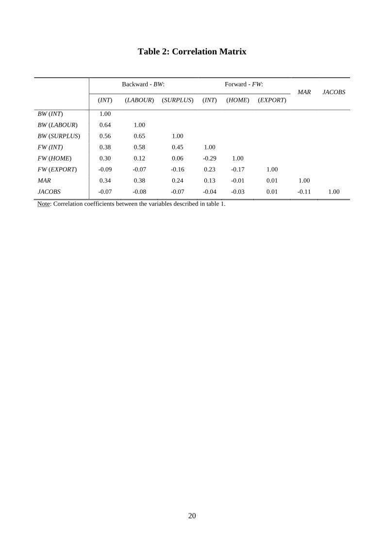
Measuring these in this way is advantageous as it reduces the correlation between the linkage

terms, which can undermine work in this area (see Amiti and Javorcik, 2008). An alternative

is to specify ekr as the industry-region employment level Ekr, but as large regions tend to have

more employees in each industry then this induces correlation.12

The correlation coefficients

between the agglomeration terms are reported in table 2, based on (10). For the backward

and forward intermediate terms the correlation coefficient is 0.38, although 0.76 when ekr =

Ekr, while otherwise the correlation coefficients are not on the high side.13

4.2 Non-intermediate goods

The UK Supply and Use Table identifies the gross value added of an industry, disaggregated

according to employee compensation (LABOUR) and the gross operating surplus (SURPLUS).

These are used to construct two backward non-intermediate terms (G = 2):14

this is also employed for an analysis at 1997. Constructing coefficients for each year is onerous, while in any

case there is the issue of years prior to 1995. The results by sub-period are considered below. 11

The invariance of the input-output coefficients is reflected in the fact that UK I/O tables are sometimes used

in the context of other countries (e.g. Ellison et al, 2010; Mariotti et al, 2010). Of course, the I/O relationships

are not purely technical relationships, and reflect factor and goods prices, but these are also reflected in the ekr. 12

At 2005, most regions had a UK GDP share in the range 7-10%, except that the South East region share was

32.0%, while the smallest region was North East England, with a 3.5% share of national output. 13

They reach up to 0.65 for some of the backward terms, but still lower than 0.85 when ekr = Ekr. 14

Gross value added is the difference between total output at basic prices and total intermediate consumption at

purchasers‟ prices. The UK Supply and Use Table also disaggregates gross value added according to „taxes less

subsidies on production‟, but these are relatively trivial and so omitted. Taxes are national in nature, and terms

11

kr

K

k l

kl

l

llr e

q

a

v

LABOURLABOURBW

1

)( , and (11)

kr

K

k l

kl

l

lr eq

a

v

SURPLUSSURPLUSBW

1

)( . (12)

The first of these terms proxies the importance of labour to each industry in each region. It is

associated with the Marshallian agglomeration economy of „thick‟ labour markets, which

arises as pools of labour offer a market for industry-specific skills (Duranton and Puga, 2004).

Underlying this, there could be many potential processes, but which are not explored here.15

The second term captures the residual surplus accruing to shareholders after the payment of

intermediate goods (including raw materials and capital goods), employees and net taxes. It

measures the attractiveness of a region to an industry not captured by the other agglomeration

terms (e.g. intermediate goods, labour, knowledge spillovers, final demand and so on) or by

the control variables. It includes the natural advantages of Ellison and Glaeser (1997) that

make some regions a better location for particular industries (e.g. access to coastal areas for

shipbuilding). Following the above, the sum of (11), (12) and (2) gives (1).

As regards the forward non-intermediate terms, the Supply and Use Table defines the

final demand for products corresponding to each industry. This is used to form two forward

non-intermediate terms (H = 2) for the final home demand (HOME) and exports (EXPORT).

They are given by (A5) and (A6) in Appendix A, where these plus (A2) sum to give (A1). In

the case of exports, for a firm in industry k the forward non-intermediate variable proxies the

importance of region r as a location for exports, which, like the other terms, is based on the

behaviour of existing firms in the industry. Both forward terms capture market access effects,

although HOME is slightly different in this respect, since if firms serve major UK regional

markets from other regions then a negative sign is expected on this term.

for the regional subsidies are included below as one of the control variables. The transaction table does not

separately identify imports, so that inputs are recorded the same whether from UK or from foreign suppliers. 15

The processes include the matching of jobs and workers, greater productivity from specialization, dual-careers

for couples and the better adaption of individual establishments to idiosyncratic shocks, although Overman and

Puga (2010) attribute only the latter to the Marshallian agglomeration economy of labour pooling.

12

4.3 Knowledge spillovers

To measure the intra-industry knowledge spillovers, or MAR externalities, then like Basile et

al (2008) and other work dating back to Woodward (1992), this is measured by the number of

FDI projects in industry l that locate in region r in the preceding period t-1, i.e. MARlrt-1. It is

an indirect method that assumes that knowledge flows in proportion to the number of recently

locating FDI projects. Other approaches exist, such as patent citations (Jaffe et al, 1993) or

technology flows (Ellison et al, 2010), but ultimately these are also indirect in nature. In net

terms, knowledge flows to rather than away from domestic plants (Mariotti et al, 2010), so

that FDI location is assumed to be independent of domestic investment in this respect. Since

it is measured at the industry level it does not capture backward production linkages.

The Jacobs knowledge-based agglomeration economies arise from industrial diversity,

and can occur over large areas (Henderson et al, 1995). It can be captured in different ways,

potentially producing different results (Beaudry and Schiffauerova, 2009), but broadly these

are classified into measures that use the inverse of either the coefficient of absolute or relative

regional specialisation (see Wren and Taylor, 1999). Given that the UK national economy is

reasonably diversified across the 46 industries, then measures that are defined relative to this

may just capture „differentness‟ rather than „diversity‟, so that the following absolute measure

is used.16

This is the inverse of the mean deviation of the industry employment shares across

the K = 46 industries, where the negative sign means that a positive coefficient is expected.

Kk

krt

krt

rt

KE

E

KJACOBS

1

1. (13)

4.4 Controls and other terms

As regards the Zrt terms in (9), these are the classical location factors that are suggested by

the literature. Head et al (1995) note that it is not possible to include terms for all possible

16

If regional employment is uniformly distributed across the 46 industries then a relative measure will indicate a

diversified regional economy when the opposite is in fact the case, so the absolute measure in (13) is preferred.

Using employment makes it comparable to the linkage terms, and it is preferred to that based on the number of

enterprises used by Lee et al (2008). It is reasonable to include both manufacturing and service industries. As a

sensitivity check, the relative measure of Duranton and Puga (2000) was instead used and if anything this gave

stronger effects for Jacobs term, i.e. larger elasticities, but (13) is preferred for the reason given.

13

location factors, so that four variables are included for each of four factors that determine the

investment decision. These are for revenue, costs, the forward-looking nature of investment

and policy, the latter since FDI has been targeted by UK regional policy.17

Control terms are

measured for each region and year, for which theory offers guidance. The variables are the

same as those used by Wren and Jones (2011), where details can be found. Since they are not

the main interest, the estimates for these are not formally presented below.

Finally, to allow for the possibility that agglomeration economies go across regional

boundaries, spatial lags (SPATIAL) are included for the linkage, MAR and Jacobs terms. To

minimise the number of such terms, they are summed for each of the backward and forward

markets. As the regions are relatively large in scale, „spillovers‟ are more likely for regions

that share a common land boundary, so that the spatial weight is based on the contiguity of

regions. A positive sign indicates a positive spillover from neighbouring regions.

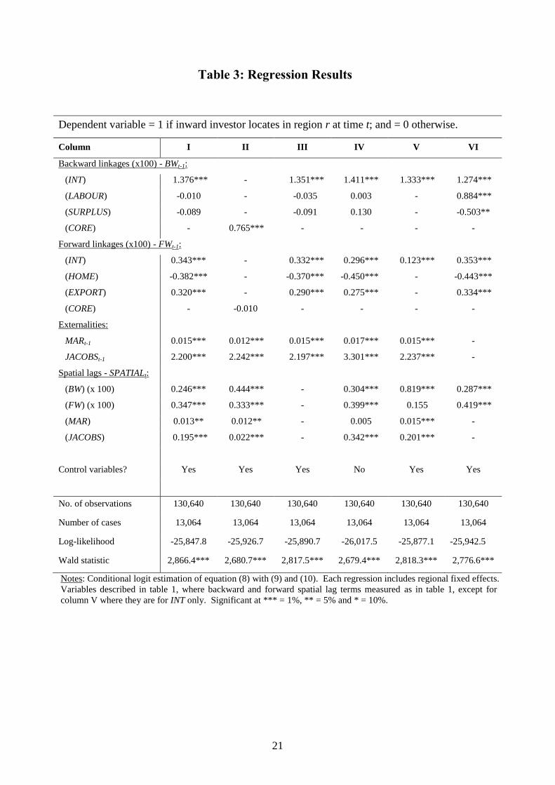
5 Regression Results

The results from the conditional logit estimation of (8) are reported in column I of table 3.

This uses the profits expression in (9), where the variables are defined in table 1. Half of the

control variables are significant, all at the 1% level, of which each is correctly signed.18

The

backward and forward intermediate terms (INT) are significant, which is also the case for the

forward non-intermediate market access terms. The negative sign on FW(HOME) indicates

that firms locate away regions with high domestic final demand for their output, and suggests

that FDI does not serve regional markets, while FW(EXPORT) shows that locations with high

industry exports are more attractive to FDI, suggesting that they serve international markets.

However, both backward non-intermediate terms, BW(LABOUR) and BW(SURPLUS), are

insignificant. The knowledge terms are significant and correctly signed, and the spatial lags

17

For the revenue that can be earned in a region, terms are included for the population size, per capita income,

distance to major markets and education qualifications, the latter to capture knowledge in general. The variables

for costs are the wage rate, availability of unskilled labour and terms for access and congestion based on road

data. For regional prospects they are the growth rate, the proportion of strikes, and indicators of development

(one based on unemployment and the other on the European regional policy spending, including infrastructure).

Finally, policy terms are expenditure on UK regional investment grants (of which half goes to FDI), the grant

rate applied in each region, a spatial lag term to pick-up regional competition for projects and the involvement

of UKTI in each region to capture the non-financial support for FDI. The spatial lag is based on the amount of

grant going to contiguous regions, arising from the regional administration of the national grant scheme. 18

They cover each of the four factors, comprising population size, distance to major markets, knowledge, access,

congestion, growth rate, grant amount and FDI promotion. Full results are available from the authors.

14

indicate that regional spillovers are present for each kind of agglomeration economy.

Column II of table 3 reports the estimates for when the linkage terms are constructed

using the core input-output table only, i.e. (1) and (A1). These constrain the estimates on the

respective intermediate and non-intermediate terms to be the same, and give different results.

Hence, compared to the estimates for the intermediate goods terms in column I, a smaller but

significant estimate is obtained for the backward linkage term and an insignificant estimate is

found for the forward term. This confirms that in constructing the terms for the intermediate

goods markets care should be taken over the choice of the appropriate denominator. In fact,

the constraints imposed by (1) and (A1) are heavily rejected by the data.19

Examination indicates that a single lag on the right-hand side terms of (9) is optimal,

while the other columns in table 3 carry out sensitivity tests of the regression result in column

I.20

In columns III and IV the spatial lags and control variables are dropped, but the estimates

on the linkage and spillover terms are robust. In column V the non-intermediate goods terms

are omitted (spatial lags are measured for the intermediate terms only), but again the results

are robust, except that a lower estimate is found for the forward intermediate term. Finally,

column VI drops the MAR and JACOBS terms (and associated spatial lags) and the backward

non-intermediate terms BW(LABOUR) and BW(SURPLUS) are now significant, although the

latter has a negatively-signed coefficient. This seems to be related to the MAR spillover term,

for which there are several possible explanations.

The first is that the two linkage terms depend on MAR, so that they are endogenous.21

As MAR is measured by the number of FDI projects, then variations in this may be expected

to affect the total number of employees and total surplus earned in a region. However, as an

explanation this is doubtful, as LABOUR and SURPLUS are drawn from the 1995 Supply and

Use Table, whereas the vast majority of projects are after this time. Further, while MAR may

affect these backward non-intermediate terms through the regional employment structure ekr,

the terms in square brackets in (11) and (12) that include ekr are just BW(INT) in (2), but the

estimate on this term is robust to the different specifications in table 3.

The more plausible explanation is that there is multicollinearity between MAR and the

backward non-intermediate goods terms BW(LABOUR) and BW(SURPLUS), despite MAR

19

The LR test statistic is 157.8 against a 2 critical value of 13.3 at the 1% level.

20 Introducing a further lag on the right-hand side terms in (9) gives more or less identical estimates for the

agglomeration terms, except that those for MAR and JACOBS are smaller. It gives a smaller log-likelihood at -

25,868.1, compared to -25,847.8 in column I of table 3, so that a single lag is preferred. 21

We rule the other possibility, that MAR depends on BW(LABOUR) and BW(SURPLUS), as the estimates on

the other linkage terms in table 3 are robust to the exclusion of MAR in column VI of table 3. Attempts to assess

the exogeneity of the variables using a Hausman test were unsuccessful due to collinearity.

15

not exhibiting a high correlation with either of these in table 2.22

This is because industries

that have both a high labour content and greater surplus will tend to be in services, but which

have received greater levels of FDI, particularly since the late 1990s (Jones and Wren, 2006).

It suggests that manufacturing and service industries should be considered separately, and

indeed when this is done below it is found that not only is the estimate of MAR significantly

different between these, but the backward non-intermediate goods terms appear to be much

better determined. It suggests that the multicollinearity is much reduced, although it may not

be eliminated altogether, as a structural break exists for each sector related to the backward

non-intermediate goods terms, but not as great as for all industry.23

5.1 By industrial sector

The estimated coefficients on the agglomeration terms from regressing column I of table 3

with dummies on these terms for industries in each of the manufacturing and service sectors

are reported in part (a) of table 4. The row for All Industry in this table reproduces the results

from column I of table 3. When taken as a group the null hypothesis that the estimates on the

agglomeration terms are the same across sectors is heavily rejected by the data.24

Further,

when examined individually, four agglomeration terms differ significantly between sectors

(the first of these at the 5% level and others at the 1% level): the backward intermediate term,

BW(INT); the forward non-intermediate term for domestic demand, FW(HOME); and the two

spillover terms, MAR and JACOBS. The backward non-intermediate goods terms are each

positive and generally significant, but do not differ statistically between the sectors.

To assess the relative importance of the agglomeration terms it is possible to evaluate

elasticities. These are for the change in the probability of FDI location at the regional level

with respect to the change in the respective agglomeration term. Letting P denote the mean

probability that a firm chooses a location (evaluated across firms, regions and time) and A

22

In support of this, if MAR is lagged a further period in column I of table 3 then BW(LABOUR) is significant at

the 5% level (a coefficient of 0.310), while BW(SURPLUS) continues to be insignificant (a p-value of 0.44). 23

Column I of table 3 was regressed with dummies on the intermediate and non-intermediate linkage terms for

the sub-period 1996-07. The LR statistic for the null hypothesis that these slope dummies are jointly zero is

47.4, against a 2(6) critical value of 16.8 at the 1% level. Examination shows that it is related to the backward

non-intermediate goods terms. When the same test was carried out for projects in the manufacturing and service

industries only, the statistics are 23.8 and 27.7 respectively, where the same critical value applies. The input-

output coefficients are measured at 1995, but given that the structural break relates to the backward non-

intermediate goods terms only then this seems to relate to the different nature of FDI from the mid-1990s when

service-based FDI was much more prominent and grew strongly. 24

The LR test statistic is 256.6 against a 2(16) critical value of 32.0 at the 1% level.

16

the mean of an agglomeration term then the marginal effect from (7) is 1 PPAP ,

so that the elasticity can be calculated as:

1 PAP

A

A

P

. (14)

The elasticities are presented in part (b) of table 4 (each is multiplied by 100). They show

that the backward intermediate goods are more important for manufacturing and that forward

intermediate goods are more important for services (although only the former is significantly

different by the above). For non-intermediate goods a different pattern emerges, as backward

effects are now more important for services, while for manufacturing UK regional markets

are even less important and export markets are more important. Finally, there are significant

differences in the MAR and Jacobs knowledge terms between industrial sectors that indicate

differences in the nature of knowledge transfer. While larger effects are generally found in

the literature for MAR compared to Jacobs externalities (Beaudry and Schiffauerova, 2009),

much of this evidence is for manufacturing, but these results suggest that the opposite is the

case for services, where knowledge is more transferable across industries.

The elasticities were also evaluated for manufacturing and services for each region by

allowing P and A to vary according to these. Space constraints prevent the presentation of

these estimates, which are available from the authors on request. Overall, they indicate very

similar effects, except where they vary strongly they add plausibility to the results concerning

the effect of particular agglomeration terms. For example, in the case of the externality terms

the elasticities for the Jacobs term are greater in the more diversified regional economies of

the East and East Midlands regions (at 25% and 21%), while that for the MAR term is greater

in the large South East region (at 28%). In relation to the South East region a slope dummy

was placed on FW(HOME) for this region to allow for its relatively large market size. This

was positive and significant, while the estimate on this term for all the regions continued to

be negative, albeit smaller and significant at the 10% level only. It suggests that the negative

coefficient on FW(HOME) in table 4 to some extent reflects access to this market.

5.2 By industry

Finally, the agglomeration effects were explored at the individual industry level. This poses

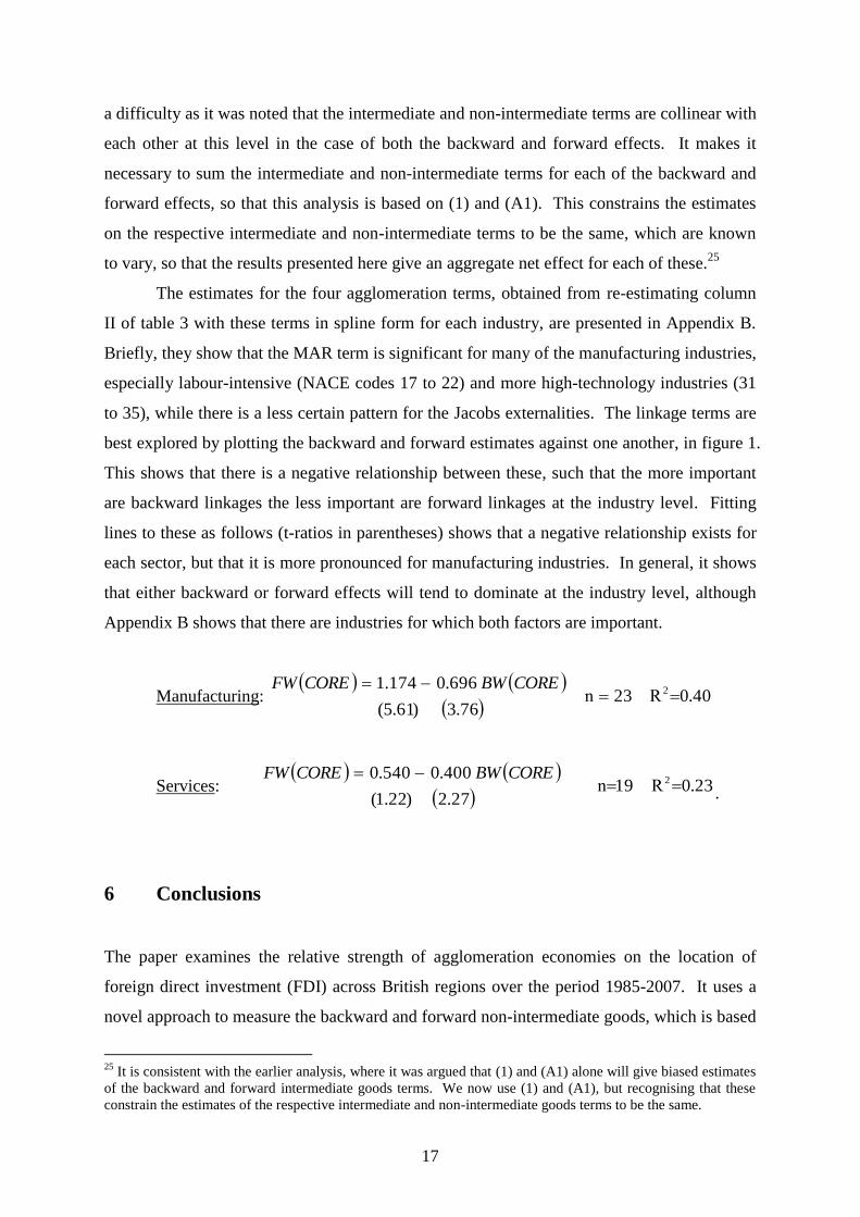
17

a difficulty as it was noted that the intermediate and non-intermediate terms are collinear with

each other at this level in the case of both the backward and forward effects. It makes it

necessary to sum the intermediate and non-intermediate terms for each of the backward and

forward effects, so that this analysis is based on (1) and (A1). This constrains the estimates

on the respective intermediate and non-intermediate terms to be the same, which are known

to vary, so that the results presented here give an aggregate net effect for each of these.25

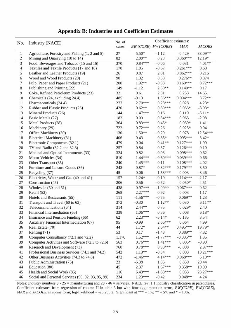
The estimates for the four agglomeration terms, obtained from re-estimating column

II of table 3 with these terms in spline form for each industry, are presented in Appendix B.

Briefly, they show that the MAR term is significant for many of the manufacturing industries,

especially labour-intensive (NACE codes 17 to 22) and more high-technology industries (31

to 35), while there is a less certain pattern for the Jacobs externalities. The linkage terms are

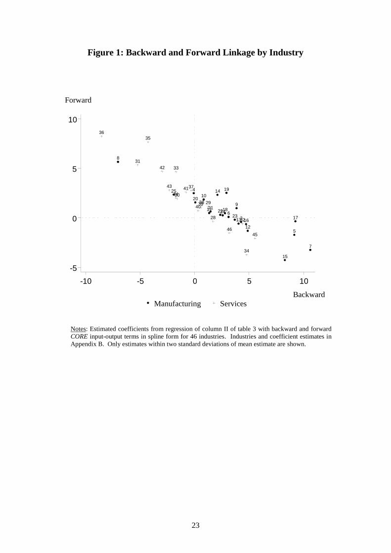
best explored by plotting the backward and forward estimates against one another, in figure 1.

This shows that there is a negative relationship between these, such that the more important

are backward linkages the less important are forward linkages at the industry level. Fitting

lines to these as follows (t-ratios in parentheses) shows that a negative relationship exists for

each sector, but that it is more pronounced for manufacturing industries. In general, it shows

that either backward or forward effects will tend to dominate at the industry level, although

Appendix B shows that there are industries for which both factors are important.

Manufacturing:

40.023

76.3)61.5(

696.0174.12

Rn

COREBWCOREFW

Services:

23.019

27.2)22.1(

400.0540.02

Rn

COREBWCOREFW

.

6 Conclusions

The paper examines the relative strength of agglomeration economies on the location of

foreign direct investment (FDI) across British regions over the period 1985-2007. It uses a

novel approach to measure the backward and forward non-intermediate goods, which is based

25

It is consistent with the earlier analysis, where it was argued that (1) and (A1) alone will give biased estimates

of the backward and forward intermediate goods terms. We now use (1) and (A1), but recognising that these

constrain the estimates of the respective intermediate and non-intermediate goods terms to be the same.

18

on an Input-Output transaction table that is on a comparable basis to the more usual proxies

for intermediate goods. The paper finds that production linkages and knowledge spillovers

explain location, but that when measured as elasticities the former are more important, which

offers support for the New Economic Geography explanation for industrial location over the

New Growth Theory based on knowledge spillovers. The effects vary between manufacturing

and service industries, such that backward intermediate goods markets are more important for

manufacturing and forward intermediate goods markets for services, while the converse tends

to be the case for non-intermediate goods markets. The transferability of knowledge, whether

intra- or inter-industry, also varies in relative importance between these sectors.

Overall, the paper produces interesting and plausible findings on the relative effects of

agglomeration economies, and points to interesting differences between these at the level of

the industrial sector. It makes a contribution to methodology, since as a guide to future work

it suggests that the full range of terms for agglomeration economies should be included and

that the intermediate goods should be measured in an appropriate way, while it also proposes

an approach for proxying the non-intermediate inputs and outputs at the sub-national industry

level. Taking all of these factors into the account, the conclusion of the paper is that the New

Economic Geography provides a more powerful explanation for location than does the New

Growth Theory based on knowledge spillovers. This is based on the location of FDI at the

UK regional level, so that it interesting to be seen if these findings apply elsewhere.

19

Table 1: Variables

Variable label Description Mean s.d.

Backward linkages for industry l in region r at time t (x 100) - BWlrt:

(INT) Intermediate goods, defined by equation (2). 1.089 0.407

(LABOUR) Compensation of employees, by (11). 0.818 0.639

(SURPLUS) Gross operating surplus, by (12). 0.438 0.345

(CORE) Core input-output linkages, by (1). 2.301 1.192

Forward linkages for industry l in region r at time t (x 100) - FWlrt:

(INT) Intermediate goods, measured by equation (A2). 1.704 1.084

(HOME) Domestic non-firm demand, by (A5). 1.242 1.206

(EXPORT) Export demand, by (A6). 0.566 0.574

(CORE) Core input-output linkages, by (A1). 3.254 1.634

Externalities:

MARlrt Number of industry l projects in region r at time t. 0.332 0.834

JACOBSrt Diversity of activity in r at time t, by (13). 4.773 6.484

Spatial lags using contiguity as weight for industry l in region r at time t - SPATIALlrt:

(BW) Measured according to (1) (x 100). 2.659 0.763

(FW) Measured according to (A1) (x 100). 3.532 1.076

(MAR) Measured by number of own-industry projects. 1.664 1.440

(JACOBS) Measured according to (13) x 100. 3.302 0.242

Note: Means and standard deviation (s.d.) calculated across 13,064 observations.

Sources: Backward and forward terms from Supply and Use Tables (ONS, 2007) and National

Online Manpower Information Service (NOMIS), Office for National Statistics, Newport. JACOBS

constructed using NOMIS data, and MAR based on FDI project data supplied by UK Trade and

Industry, HM Government, London.

20

Table 2: Correlation Matrix

Backward - BW: Forward - FW:

MAR JACOBS (INT) (LABOUR) (SURPLUS) (INT) (HOME) (EXPORT)

BW (INT) 1.00

BW (LABOUR) 0.64 1.00

BW (SURPLUS) 0.56 0.65 1.00

FW (INT) 0.38 0.58 0.45 1.00

FW (HOME) 0.30 0.12 0.06 -0.29 1.00

FW (EXPORT) -0.09 -0.07 -0.16 0.23 -0.17 1.00

MAR 0.34 0.38 0.24 0.13 -0.01 0.01 1.00

JACOBS -0.07 -0.08 -0.07 -0.04 -0.03 0.01 -0.11 1.00

Note: Correlation coefficients between the variables described in table 1.

21

Table 3: Regression Results

Notes: Conditional logit estimation of equation (8) with (9) and (10). Each regression includes regional fixed effects.

Variables described in table 1, where backward and forward spatial lag terms measured as in table 1, except for

column V where they are for INT only. Significant at *** = 1%, ** = 5% and * = 10%.

Dependent variable = 1 if inward investor locates in region r at time t; and = 0 otherwise.

Column I II III IV V VI

Backward linkages (x100) - BWt-1:

(INT) 1.376*** - 1.351*** 1.411*** 1.333*** 1.274***

(LABOUR) -0.010 - -0.035 0.003 - 0.884***

(SURPLUS) -0.089 - -0.091 0.130 - -0.503**

(CORE) - 0.765*** - - - -

Forward linkages (x100) - FWt-1:

(INT) 0.343*** - 0.332*** 0.296*** 0.123*** 0.353***

(HOME) -0.382*** - -0.370*** -0.450*** - -0.443***

(EXPORT) 0.320*** - 0.290*** 0.275*** - 0.334***

(CORE) - -0.010 - - - -

Externalities:

MARt-1 0.015*** 0.012*** 0.015*** 0.017*** 0.015*** -

JACOBSt-1 2.200*** 2.242*** 2.197*** 3.301*** 2.237*** -

Spatial lags - SPATIALt:

(BW) (x 100) 0.246*** 0.444*** - 0.304*** 0.819*** 0.287***

(FW) (x 100) 0.347*** 0.333*** - 0.399*** 0.155 0.419***

(MAR) 0.013** 0.012** - 0.005 0.015*** -

(JACOBS) 0.195*** 0.022*** - 0.342*** 0.201*** -

Control variables? Yes Yes Yes No Yes Yes

No. of observations 130,640 130,640 130,640 130,640 130,640 130,640

Number of cases 13,064 13,064 13,064 13,064 13,064 13,064

Log-likelihood -25,847.8 -25,926.7 -25,890.7 -26,017.5 -25,877.1 -25,942.5

Wald statistic 2,866.4*** 2,680.7*** 2,817.5*** 2,679.4*** 2,818.3*** 2,776.6***

22

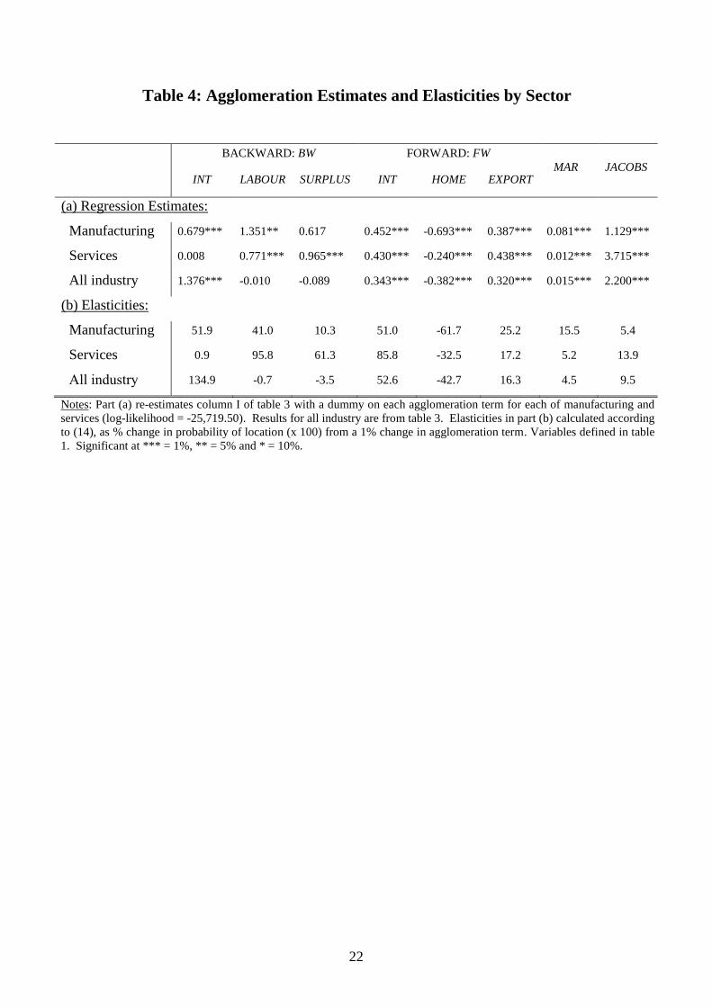
Table 4: Agglomeration Estimates and Elasticities by Sector

BACKWARD: BW FORWARD: FW

MAR JACOBS INT LABOUR SURPLUS INT HOME EXPORT

(a) Regression Estimates:

Manufacturing 0.679*** 1.351** 0.617 0.452*** -0.693*** 0.387*** 0.081*** 1.129***

Services 0.008 0.771*** 0.965*** 0.430*** -0.240*** 0.438*** 0.012*** 3.715***

All industry 1.376*** -0.010 -0.089 0.343*** -0.382*** 0.320*** 0.015*** 2.200***

(b) Elasticities:

Manufacturing 51.9 41.0 10.3 51.0 -61.7 25.2 15.5 5.4

Services 0.9 95.8 61.3 85.8 -32.5 17.2 5.2 13.9

All industry 134.9 -0.7 -3.5 52.6 -42.7 16.3 4.5 9.5

Notes: Part (a) re-estimates column I of table 3 with a dummy on each agglomeration term for each of manufacturing and

services (log-likelihood = -25,719.50). Results for all industry are from table 3. Elasticities in part (b) calculated according

to (14), as % change in probability of location (x 100) from a 1% change in agglomeration term. Variables defined in table

1. Significant at *** = 1%, ** = 5% and * = 10%.

23

Figure 1: Backward and Forward Linkage by Industry

Notes: Estimated coefficients from regression of column II of table 3 with backward and forward

CORE input-output terms in spline form for 46 industries. Industries and coefficient estimates in

Appendix B. Only estimates within two standard deviations of mean estimate are shown.

3

4

5

6

7

8

9 10

11

12 13

14

15

16 17 18

19

20

21 22

23 24

25

28

29 30

31

32

33

34

35 36

37

38 39 40

41

42

43 44

45 46

-5

0

5

10

-10 -5 0 5 10

Backward

Manufacturing Services

Forward

24

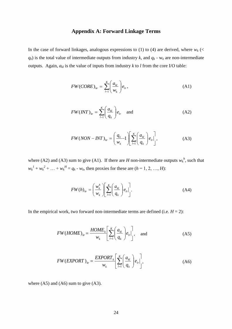
Appendix A: Forward Linkage Terms

In the case of forward linkages, analogous expressions to (1) to (4) are derived, where wk (<

qk) is the total value of intermediate outputs from industry k, and qk - wk are non-intermediate

outputs. Again, akl is the value of inputs from industry k to l from the core I/O table:

lr

K

l k

klkr e

w

aCOREFW

1

)( , (A1)

lr

K

l k

klkr e

q

aINTFW

1

)( and (A2)

lr

K

l k

kl

k

kkr e

q

a

w

qINTNONFW

1

1)( , (A3)

where (A2) and (A3) sum to give (A1). If there are H non-intermediate outputs wkh, such that

wk1 + wk

2 + … + wk

H = qk - wk, then proxies for these are (h = 1, 2, …, H):

lr

K

l k

kl

k

h

kkr e

q

a

w

whFW

1

)( . (A4)

In the empirical work, two forward non-intermediate terms are defined (i.e. H = 2):

lr

K

l k

kl

k

kkr e

q

a

w

HOMEHOMEFW

1

)( , and (A5)

lr

K

l k

kl

k

kkr e

q

a

w

EXPORTEXPORTFW

1

)( , (A6)

where (A5) and (A6) sum to give (A3).

25

Appendix B: Industries and Coefficient Estimates

No. Industry (NACE) No. of

cases

Coefficient estimates:

BW (CORE) FW (CORE) MAR JACOBS

1 Agriculture, Forestry and Fishing (1, 2 and 5) 27 5.50* -1.12 -0.429 33.09**

2 Mining and Quarrying (10 to 14) 82 2.00** 0.23 0.360*** 12.19*

3 Food, Beverages and Tobacco (15 and 16) 370 0.84*** -0.06 0.031 4.01**

4 Textiles and Textile Products (17 and 18) 170 1.05 -0.67 0.261*** 0.68

5 Leather and Leather Products (19) 26 0.87 2.01 0.862*** 0.216

6 Wood and Wood Products (20) 90 1.32 0.58 0.276** 0.874

7 Pulp, Paper and Paper Products (21) 200 1.92** -0.33 0.169*** 8.72***

8 Publishing and Printing (22) 149 -1.12 2.50** 0.140** 0.17

9 Coke, Refined Petroleum Products (23) 32 0.61 2.31 0.253 14.65

10 Chemicals (24, excluding 24.4) 485 -0.13 1.36*** 0.094*** 3.72**

11 Pharmaceuticals (24.4) 277 2.70*** 0.28*** 0.028 4.23*

12 Rubber and Plastic Products (25) 420 0.62** 0.89*** 0.055* -3.03*

13 Mineral Products (26) 144 1.47*** 0.16 0.119 -5.11*

14 Basic Metals (27) 182 0.09 0.84*** 0.065 -2.08

15 Metal Products (28) 364 0.83*** 0.45* 0.059* 1.41

16 Machinery (29) 722 0.72*** 0.26 0.025* 0.04

17 Office Machinery (30) 130 1.50** -0.29 0.078 12.54***

18 Electrical Machinery (31) 406 0.43 0.85* 0.095*** 3.42*

19 Electronic Components (32.1) 479 -0.04 0.41** 0.127*** 1.99

20 TV and Radio (32.2 and 32.3) 257 0.84 0.37 0.126*** 0.10

21 Medical and Optical Instruments (33) 324 0.82 -0.03 0.098*** 0.62

22 Motor Vehicles (34) 810 1.44*** -0.60*** 0.039*** 0.66

23 Other Transport (35) 240 1.45*** 0.11 0.108*** 4.02

24 Furniture and Leisure Goods (36) 243 0.87* 0.82*** 0.179*** 3.50

25 Recycling (37) 45 -0.06 1.53*** 0.003 -3.46

26 Electricity, Water and Gas (40 and 41) 157 1.24* -0.19 0.114*** -2.17

27 Construction (45) 206 0.56 -0.52 0.050* 4.51

28 Wholesale (50 and 51) 438 0.97*** -1.09** 0.067*** 0.62

29 Retail (52) 268 2.27*** 0.92 0.003 1.17

30 Hotels and Restaurants (55) 111 -1.56*** -0.75 0.069** 1.23

31 Transport and Travel (60 to 63) 373 -0.30 1.12** 0.030 6.11**

32 Telecommunications (64) 314 2.44** 0.75 0.029* 2.40

33 Financial Intermediation (65) 338 1.06*** 0.56 0.008 6.18*

34 Insurance and Pension Funding (66) 62 2.23*** -5.14* -0.185 3.54

35 Auxiliary Financial Intermediation (67) 95 -0.99 2.66*** 0.064 4.99

36 Real Estate (70) 44 1.72* 2.64** 0.495*** 19.79*

37 Renting (71) 53 0.17 -1.43 0.389** 7.82

38 Computer Consultancy (72.1 and 72.2) 1,176 1.52*** -1.77*** -0.005** 1.35

39 Computer Activities and Software (72.3 to 72.6) 563 0.76*** 1.41*** 0.005* -0.90

40 Research and Development (73) 760 0.78*** 0.98*** -0.008 2.97***

41 Professional Business Services (74.1 and 74.2) 542 1.13** -0.34 0.003 10.21***

42 Other Business Activities (74.3 to 74.8) 472 -1.46*** 4.14*** 0.068*** 5.10**

43 Public Administration (75) 23 -6.38 1.85 0.830 20.44

44 Education (80) 45 2.37 1.67*** 0.358** 10.99

45 Health and Social Work (85) 116 6.43*** -1.88*** 0.033 23.27***

46

Social and Personal Services (90, 92, 93, 95, 99) 234 1.29*** -0.42 0.048** 4.24

Notes: Industry numbers 3 - 25 = manufacturing and 28 - 46 = services. NACE rev. 1.1 industry classification in parentheses.

Coefficient estimates from regression of column II in table 3 but with four agglomeration terms, BW(CORE), FW(CORE),

MAR and JACOBS, in spline form; log-likelihood = -25,235.2. Significant at *** = 1%, ** = 5% and * = 10%.

26

References

Alegria, R. (2009), „The Location of Multinational Firms in the UK: Sectoral and Functional

Agglomeration‟, Spatial Economics Research Centre, Annual Conference, London

School of Economics, May.

Amiti, M. and Javorcik, B. (2008), „Trade Costs and Location of Foreign Firms in China‟,

Journal of Development Economics, 85, 129-49.

Arauzo-Carod, J-M., Liviano-Solis, D. and Manjón-Antolín, M. (2010), „Empirical Studies in

Industrial Location: An Assessment of their Methods and Results‟, Journal of Regional

Science, 50.3, 685-711.

Armstrong, H. and Taylor, J. (2000), Regional Economics and Policy, Blackwell, Oxford.

Audretsch, D. and Feldman, M. (1996), „R&D Spillovers and the Geography of Innovation

and Production‟, American Economic Review, 86.3, 630-40.

Baldwin, J.R., Beckstead, D., Brown, M. and Rigby, D. (2008), „Agglomeration and the

Geography of Localization Economies in Canada‟, Regional Studies, 42.1, 117-32.

Basile, R., Castellani, D. and Zanfei, A. (2008), „Location Choices of Multinational Firms in

Europe: The Role of EU Cohesion Policy‟, Journal of International Economics, 74.2,

328-40.

Beaudry, C. and Schiffauerova (2009), „Who‟s Right, Marshall or Jacobs? The Localization

versus Urbanization Debate‟, Research Policy, 38, 318-37.

Beenstock, M. and Felsenstein, D. (2010), „Marshallian Theory of Regional Agglomeration‟,

Papers in Regional Science, 89.1, 155-72.

Bekes, G. (2006), „Location of Manufacturing FDI in Hungary: How Important are Inter-

company Relationships?‟, MNB Working Papers, The Central Bank of Hungary.

Brand, S., Hill, S. and Munday, M. (2000), „Assessing the Impacts of Foreign Manufacturing

on Regional Economies: The Cases of Wales, Scotland and the West Midlands‟,

Regional Studies, 34, 343-55.

Carlton, D. (1983), „The Location and Employment Choices of New Firms: An Econometric

Model with Discrete and Continuous Endogenous Variables‟, The Review of Economic

and Statistics, 65, 440–49.

Coughlin, C., Terza, J. and Arromdee, V. (1991), „State Characteristics and the Location of

FDI within the United States‟, Review of Economics and Statistics, 73, 675–83.

Crozet, M., Mayer, T. and Mucchielli, J-L. (2004), „How Do Firms Agglomerate? A Study of

FDI in France‟, Regional Science and Urban Economics, 34, 27-54.

Dahlberg, M. and Eklöf, M. (2003), „Relaxing the IIA Assumption in Locational Choice

Models: A Comparison between Conditional Logit, Mixed Logit, and Multinomial Probit

Models‟, Working Paper 2003.9, Department of Economics, Uppsala University.

Debaere, P., Lee, J. and Paik, M. (2010), „Agglomeration, Backward and Forward Linkages:

Evidence from South Korean Investment in China‟, Canadian Journal of Economics,

43.2, 520-46.

Devereux, M. P., Griffith, R. and Simpson, H. (2007), „Firm Location Decisions, Regional

Grants and Agglomeration Economies‟, Journal of Public Economics, 91, 413-35.

Dimitropoulou, D., Burke, S. and McCann, P. (2006), „The Determinants of the Location of

Foreign Direct Investment in UK Regions‟, Regional Science Association International:

British and Irish Section, Annual Conference, Jersey, Channel Islands, August.

Döring, T. and Schnellenbach, J. (2006), „What Do We Know about Geographical

Knowledge Spillovers and Regional Growth? A Survey of the Literature‟, Regional

Studies, 40.3, 375-95.

27

Driffield, N., Munday, M. and Roberts, A. (2004), „Inward Investment, Transaction Linkages

and Productivity Spillovers‟, Papers in Regional Science, 83, 699-722.

Du, J., Lu, Y. and Tao, Z. (2008), „FDI Location Choice: Agglomeration vs Institutions‟,

International Journal of Finance and Economics, 13, 92-107.

Duranton, G. and Puga, D. (2000), „Diversity and Specialisation in Cities: Why, Where and

When Does it Matter?‟, Urban Studies, 37.3, 533-55.

Duranton, G. and Puga, D. (2004) „Micro-Foundations of Urban Agglomeration Economies‟,

in Henderson, J. V. and Thisse, J-F, (eds), Handbook of Regional and Urban Economics:

Cities and Geography, Volume 4, North-Holland, Amsterdam.

Ellison, G. and Glaeser, E. L. (1997), „Geographic Concentration in US Manufacturing

Industries: A Dartboard Approach‟, Journal of Political Economy, 105.5, 889-927.

Ellison, G., Glaeser, E.L. and Kerr, W. (2010). „What Causes Industry Agglomeration?

Evidence from Coagglomeration Patterns‟, American Economic Review, 100.3, 1195-

1213.

Greene, W. (2011), Econometric Analysis, 7th

edition, Pearson, New York.

Griliches, Z. (1992), „The Search for R&D Spillovers‟, The Scandinavian Journal of

Economics, Supplement, 94, 29-47

Head, K, and Mayer, T. (2004), „Market Potential and the Location of Japanese Investment in

the European Union‟, Review of Economics and Statistics, 86.4, 959–72.

Head, K., Ries, J. and Swenson, D. (1995), Agglomeration Benefits and Location Choice:

Evidence from Japanese Manufacturing Investments in the United States, Journal of

International Economics, 38, 223-47.

Head, K., Ries, J. and Swenson, D. (1999), Attracting Foreign Manufacturing: Investment

Promotion and Agglomeration, Regional Science and Urban Economics, 29, 197-218.

Henderson, J.V. (2003), „Marshall‟s Scale Economies‟, Journal of Urban Economics, 53.1,

1-28.

Henderson, V., Kuncoro, A. and Turner, M. (1995), „Industrial Development in Cities‟, The

Journal of Political Economy, 103.5, 1067-90.

Hilber, C. and Voicu, I. (2007), „Agglomeration Economies and the Location of Foreign

Direct Investment: Empirical Evidence from Romania‟, Munich Personal RePEc Archive

Paper No.5137.

Jaffe, A., Trajtenberg, M. and and Henderson, R. (1993), „Geographic Localization of

Knowledge Spillovers as Evidenced by Patent Citations‟, Quarterly Journal of

Economics, 108.3, 577-98.

Javorcik, B. (2004), „Does Foreign Direct Investment Increase the Productivity of Domestic

Firms? In Search of Spillovers through Backward Linkages‟, American Economic

Review, 94.3, 605-27.

Javorcik, B. and Spatareanu, M. (2009), „Tough Love: Do Czech Suppliers Learn from their

Relationships with Multinationals?‟, Scandinavian Journal of Economics, 111:4, 811-33.

Jones, J. and Wren, C. (2004), „Do Inward Investors Achieve their Job Targets?‟, Oxford

Bulletin of Economics and Statistics, 66. 4, 483-513.

Jones, J. and Wren, C. (2006), Foreign Direct Investment and the Regional Economy,

Ashgate Press, Aldershot.

Jones, J. and Wren, C. (2011), „FDI Location across British Regions and Agglomerative

Forces: A Markov Analysis‟, mimeo.

Krugman, P. (1991), „Increasing Returns and Economic Geography‟, Journal of Political

Economy, 99.3, 483-99

Lamorgese, A. and Ottaviano, G. (2002), „Space, Factors and Spillovers‟, Banca d’Italia.

28

Lee, K-D., Hwang, S-K and Lee, M-H (2008), „Agglomeration Economies and Location

Choice of Inward Foreign Direct Investment in Korea‟, Regional Studies Association

Conference, Prague, Czech Republic, May.

Liao, T. (1994), Interpreting Probability Models: Logit, Probit and other Generalized Linear

Models, Sage, London.

Mariotti, S., Piscitello, L. and Elia, S. (2010), „Spatial Agglomeration of Multinational

Enterprises: The Role of Information Externalities and Knowledge Spillovers‟, Journal

of Economic Geography, 10.4, 519-38.

Marshall, A. (1920), Principles of Economics, Macmillan, London.

McFadden, D. (1974), „Conditional Logit Analysis of Qualitative Choice Behaviour‟, in

Zarembka, P, (eds), Frontiers in Econometrics. Academic Press, New York.

Milner, C., Reed, G. and Talerngsri, P. (2006), „Vertical Linkages and Agglomeration Effects

in Japanese FDI in Thailand‟, Journal of Japanese International Economics, 20, 193-208.

Mucchielli, J-L. and Puech, F. (2004), „Globalisation, Agglomeration and FDI Location: The

Case of French Firms in Europe‟ in Mucchielli, J-L. and Mayer, T, (eds), Multinational

Firms’ Location and the New Economic Geography, Edward Elgar, Cheltenham.

ONS (2006), United Kingdom Input-Output Analyses, edited by Sanjiv Mahajan, Office for

National Statistics, Newport, UK.

ONS (2007), Supply and Use Tables, Office for National Statistics, Newport, UK.

Overman, H. G. and Puga, D. (2010), „Labour Pooling as a Source of Agglomeration: An

Empirical Investigation‟, in Glaeser, E.L, (eds), Agglomeration Economics, University of

Chicago Press, Chicago.

Procher, V. (2009), „FDI Location Choices: Evidence from French First-time Movers‟, Wirt

Sozialstat Archiv, 3.3, 209-20.

Rosenthal, S. and Strange, W. (2001), „The Determinants of Agglomeration‟, Journal of

Urban Economics, 50.2,191-229.

Rosenthal, S. S. and Strange, W. (2004), „Evidence on the Nature and Sources of

Agglomeration Economies‟, in Henderson, J. V. and Thisse, J-F, (eds), Handbook of

Regional and Urban Economics: Cities and Geography, Volume 4, North-Holland,

Amsterdam.

Venables, A. J. (1996), „Equilibrium Locations of Vertically Linked Industries‟, International

Economic Review, 37.2, 341-59.

Wheeler, D. and Mody, A. (1992), „International Investment Location Decisions: The Case of

US Firms‟, Journal of International Economics, 33, 56–76.

Woodward, D. (1992), „Locational Determinants of Japanese Manufacturing Start-Ups in the

United States‟, Southern Economic Journal, 58, 690–708.

Wren, C. and Taylor, J. (1999), „Industrial Restructuring and Regional Policy‟, Oxford

Economic Papers, 51, 487-516.

Wren, C. and Jones, J. (2009), „Re-investment and the Survival of Foreign-owned Plants‟,

Regional Science and Urban Economics, 39, 214-23.

Wren, C. and Jones, J. (2011), „Assessing the Regional Impact of Grants on FDI Location:

Evidence from UK Regional Policy, 1985-05‟, Journal of Regional Science, 51, 497-517.

Spatial Economics Research Centre (SERC)London School of EconomicsHoughton StreetLondon WC2A 2AE

Tel: 020 7852 3565Fax: 020 7955 6848Web: www.spatialeconomics.ac.uk

SERC is an independent research centre funded by theEconomic and Social Research Council (ESRC), Departmentfor Business Innovation and Skills (BIS), the Department forCommunities and Local Government (CLG) and the WelshAssembly Government.