FE-ANN BASED MODELING OF 3D SIMPLE REINFORCED CONCRETE GIRDERS FOR

OBJECTIVE STRUCTURAL HEALTH EVALUATION

by

ERIC MATTHEW FLETCHER

B.S., Kansas State University, 2014

A THESIS

submitted in partial fulfillment of the requirements for the degree

MASTER OF SCIENCE

Department of Civil Engineering

College of Engineering

KANSAS STATE UNIVERSITY

Manhattan, Kansas

2016

Approved by:

Major Professor

Hayder A. Rasheed

Copyright

ERIC FLETCHER

2016

Abstract

The structural deterioration of aging infrastructure systems is becoming an increasingly

important issue worldwide. To compound the issue, economic strains limit the resources

available for repair or replacement of such systems. Over the past several decades, structural

health monitoring (SHM) has proved to be a cost-effective method for detection and evaluation

of damage in structures. Visual inspection and condition rating is one of the most commonly

applied SHM techniques, but the effectiveness of this method suffers due to its reliance on the

availability and experience of qualified personnel performing largely qualitative damage

evaluations. The artificial neural network (ANN) approach presented in this study attempts to

augment visual inspection methods by developing a crack-induced damage quantification model

for reinforced concrete bridge girders that requires only the results of limited field measurements

to operate. Simply-supported three-dimensional reinforced concrete T-beams with varying

geometric, material, and cracking properties were modeled using Abaqus finite element (FE)

analysis software. Up to five cracks were considered in each beam, and the ratios of stiffness

between cracked and healthy beams with the same geometric and material parameters were

measured at nine equidistant nodes along the beam. Two feedforward ANNs utilizing

backpropagation learning algorithms were then trained on the FE model database with beam

properties serving as inputs for both neural networks. The outputs for the first network consisted

of the nodal stiffness ratios, and the sole output for the second ANN was a health index

parameter, computed by normalizing the area under the stiffness ratio profile over the span

length of the beam. The ANNs achieved excellent prediction accuracies with coefficients of

determination (R2) exceeding 0.99 for both networks. Additional FE models were created to

further assess the networks’ prediction capabilities on data not utilized in the training process.

The ANNs displayed good prediction accuracies (R2 > 0.8) even when predicting damage levels

in beams with geometric, material, and cracking parameters dissimilar from those found in the

training database. A touch-enabled user interface was developed to allow the ANN models to be

utilized for on-site damage evaluations. The results of this study indicate that application of

ANNs with FE modeling shows great promise in SHM for damage evaluation.

v

Table of Contents

List of Figures ................................................................................................................................ vi

List of Tables ................................................................................................................................ vii

Acknowledgements ........................................................................................................................ ix

Chapter 1 - Introduction .................................................................................................................. 1

Background ................................................................................................................................. 1

Objectives ................................................................................................................................... 1

Scope ........................................................................................................................................... 2

Chapter 2 - Literature Review ......................................................................................................... 3

Introduction to Structural Health Monitoring ............................................................................. 3

Damage Evaluation and Structural Health Prediction Techniques ............................................. 5

Artificial Neural Networks ....................................................................................................... 15

Structure and Learning Techniques ...................................................................................... 16

Data Preparation and Training Procedure ............................................................................. 18

Optimum Model Selection Criteria ....................................................................................... 22

Chapter 3 - Methodology .............................................................................................................. 23

Generation of Reinforced Concrete Beam Database ................................................................ 23

ANN Modeling for Structural Health Prediction ...................................................................... 41

Chapter 4 - Results and Discussion .............................................................................................. 46

Chapter 5 - ANN User Interface Application ............................................................................... 59

Chapter 6 - Conclusions and Recommendations .......................................................................... 66

Conclusions ............................................................................................................................... 66

Recommendations ..................................................................................................................... 68

References ..................................................................................................................................... 70

Appendix A - Abaqus-Python Scripts........................................................................................... 74

Appendix B - Beam Width Variation Datasets ............................................................................. 84

Appendix C - Random Sample of Main Beam Database ............................................................. 88

Appendix D - Randomly Generated Testing Datasets ................................................................ 116

vi

List of Figures

Figure 2-1: General feedforward ANN structure .......................................................................... 17

Figure 2-2: Sigmoidal function plot .............................................................................................. 20

Figure 3-1: Abaqus view of 3D reinforced concrete T-beam model displaying cracks, boundary

conditions, and applied load.................................................................................................. 24

Figure 3-2: Abaqus view of 3D reinforced concrete T-beam model displaying concrete FE mesh

............................................................................................................................................... 24

Figure 3-3: Variation in beam deflection with reduction of mesh size......................................... 26

Figure 3-4: T-beam flange dimensions ......................................................................................... 29

Figure 3-5: Reinforced concrete T-beam elevation view ............................................................. 30

Figure 3-6: Graphical comparison between health indices of beams with web widths of (a) 250

mm and 200mm and (b) 250 mm and 300 mm ..................................................................... 39

Figure 3-7: Graphical description of health index ........................................................................ 42

Figure 4-1: Main database – predicted versus actual values for (a) k%1, (b) k%2, (c) k%3, ........ 54

Figure 4-2: Testing sets of beams with two, three, and four cracks – predicted versus actual

values for (a) k%1, (b) k%2, (c) k%3, (d) k%4, (e) k%5, (f) k%6, (g) k%7, (h) k%8, ............. 56

Figure 4-3: Randomly generated testing sets – predicted versus actual values for (a) k%1, (b)

k%2, (c) k%3, (d) k%4, (e) k%5, (f) k%6, (g) k%7, (h) k%8, (i) k%9, and (j) ki% .................. 57

Figure 5-1: Nodal stiffness ratio and health index prediction graphical user interface ................ 60

Figure 5-2: ANN user interface application results for test beam 1 (ANN ID 8400) ................... 63

Figure 5-3: ANN user interface application results for test beam 2 (ANN ID 43180) ................. 64

Figure 5-4: Visual Studio WPF application results for reference beam used in parameter impact

testing .................................................................................................................................... 65

vii

List of Tables

Table 3-1: Stiffness ratio comparison of sample T-beam 2D and 3D models .............................. 28

Table 3-2: Parameter variability for singly-cracked beams .......................................................... 32

Table 3-3: Parameter variability for beams with five cracks ........................................................ 33

Table 3-4: Parameter variability for additional beams with five cracks ....................................... 34

Table 3-5: Parameter variability for beams with two cracks ........................................................ 35

Table 3-6: Parameter variability for beams with three cracks ...................................................... 36

Table 3-7: Parameter variability for beams with four cracks ....................................................... 37

Table 3-8: Statistical comparisons between health indices of beams with different widths ........ 39

Table 3-9: Sample Microsoft Excel database header .................................................................... 43

Table 3-10: ANN expanded parameter ranges .............................................................................. 44

Table 4-1: Statistical results for optimal nodal stiffness ratio prediction ANNs .......................... 46

Table 4-2: Statistical results for optimal health index prediction ANNs ...................................... 47

Table 4-3: Parameter variability for additional test beams with two cracks................................. 48

Table 4-4: Parameter variability for additional test beams with three cracks............................... 49

Table 4-5: Parameter variability for additional test beams with four cracks ................................ 49

Table 4-6: Statistical results for optimal nodal stiffness ratio prediction ANNs tested on

additional data for beams with two, three, and four cracks .................................................. 50

Table 4-7: Statistical results for optimal health index prediction ANNs tested on additional data

for beams with two, three, and four cracks ........................................................................... 50

Table 4-8: Statistical results for optimal health index ANNs trained on altered database and

tested on exchanged beam sets ............................................................................................. 51

Table 4-9: Statistical results for optimal nodal stiffness ratio prediction ANNs tested on

randomly generated beams with 1–5 cracks ......................................................................... 52

Table 4-10: Statistical results for optimal health index prediction ANNs tested on randomly

generated beams with 1–5 cracks.......................................................................................... 52

Table 5-1: ANN prediction results for test beams ........................................................................ 64

Table B-1: Beam width variation datasets – geometric and material parameters and health indices

for different widths ............................................................................................................... 84

Table B-2: Beam width variation datasets – cracking parameters ................................................ 85

viii

Table C-1: Main database – geometric and material input, and nodal stiffness ratio and health

index output parameters ........................................................................................................ 88

Table C-2: Main database – cracking input parameters .............................................................. 102

Table D-1: Randomly generated testing datasets – geometric and material input, and nodal

stiffness ratio and health index output parameters .............................................................. 116

Table D-2: Randomly generated testing datasets – cracking input parameters .......................... 118

ix

Acknowledgements

I would first like to extend my deepest thanks to my advisor, Dr. Hayder Rasheed, for his

guidance and support throughout both my undergraduate and graduate studies. His mentorship

throughout this research project has helped lead it to its successful completion, and I sincerely

appreciate all of his efforts. I would also like to thank Dr. Yacoub Najjar for granting us the use

of his artificial neural network (ANN) program and for being available as our expert ANN

consultant. I also greatly appreciate Dr. Hani Melham’s involvement throughout my college

career, and I would like to thank all three of these men for serving on my MS. defense

committee.

I am very grateful for Dr. Ahmed Al-Rahmani’s involvement throughout the early stages

of this project. He helped design the methodology used in this research and taught me the ANN

and finite element (FE) scripting techniques applied in this study. I would also like to thank

Rund Al-Masri for her help in developing the 3D FE modeling approach used in this project. I

appreciate the statistical comparison advice provided by Nicholas Bloedow of the Statistical

Consulting Lab and the editing advice provided by Tamara Robinson of the Engineering

Research and Graduate Programs. I would like to extend my sincere appreciation to the Midwest

Transportation Center at Iowa State University for funding this research project.

I would like to acknowledge my friends, both at Kansas State University and elsewhere.

Their friendship is greatly appreciated, and I thank them for making my college career so

enjoyable. I would also like to thank Kaitlin Foley for her support and companionship. I am

lucky to have someone such as her in my life. Last, but certainly not least, I would like to thank

my family, and above all, my parents, for their love, support, and encouragement throughout my

entire life. Words cannot express my gratitude to them.

1

Chapter 1 - Introduction

Background

The deterioration of aging infrastructure is becoming an increasingly important issue both

domestically and abroad, especially in the midst of an uncertain economic climate. Structures

such as reinforced concrete bridges are subject to damage over time due to physical or chemical

processes. Structural health monitoring (SHM) strategies are frequently applied to bridges and

other infrastructure systems to detect, monitor, and evaluate damage, resulting in improved and

economic repair or remediation solutions. Numerous SHM techniques utilizing various

technologies have been proposed as alternatives to the subjective visual inspection and condition

rating method. Artificial neural networks (ANNs) are robust and innovative tools that

demonstrate promising potential for application in SHM.

Objectives

The primary goal of this research project was to utilize ANNs to produce a SHM model

for objective damage evaluation of reinforced concrete bridge T-girders. Initially, a reinforced

concrete beam finite element (FE) model database was generated using Abaqus FE analysis

software. Beams in the database consisted of simply-supported reinforced concrete T-beams with

varying geometric, material, and cracking parameters, and beams were modeled with zero to five

cracks by dividing the girders into five equal segments with no more than one crack per segment.

Damage was characterized by the ratios of stiffness between cracked and uncracked beams at

nine equidistant nodes, and a health index parameter was used to resolve the nodal stiffness

ratios into a single objective measure of structural health. Feedforward ANNs employing a

backpropagation learning algorithm were trained on the database to predict nodal stiffness ratios

and health indices of the beams given their geometric, material, and cracking parameters.

2

Ultimately, the optimum models from the ANN modeling process were utilized to create touch-

enabled graphical user interfaces for on-site damage evaluation applications.

Scope

This thesis is divided into six chapters. Chapter 1 introduces the background for the

research, details the objectives of the study, and summarizes the scope of the thesis. Chapter 2

provides justification for the research, discusses the practice of SHM, reviews several studies

related to SHM for damage evaluation, and introduces ANNs. Chapter 3 describes the creation of

the reinforced concrete beam FE model database and discusses the techniques used to apply

ANNs in order to create structural health prediction models. Chapter 4 presents the statistical

results from the ANN training process and optimal model selection procedure and details the

additional tests performed to assist in the selection of the top-performing damage evaluation

network architectures. Chapter 5 describes the development of the touch-enabled graphical user

interface, which allows the optimal ANN structural health prediction models to be applied in

real-world SHM investigations. Chapter 6 reviews the study, summarizes the research

conclusions, and provides recommendations for continuation and expansion of the work

performed.

3

Chapter 2 - Literature Review

Introduction to Structural Health Monitoring

Bridges are vital components of national infrastructures, and transportation systems

throughout the world depend upon their safe and reliable operation. To ensure such operation,

bridge structures require periodic maintenance and eventual rehabilitation or replacement. While

all structures require upkeep, bridges often demand more attention due to hardships endured

during their service lives. Harsh external environments, extreme loading events, and fatigue due

to service loading all induce structural damage over time. Bridges that sustain significant damage

are classified as structurally deficient, thereby indicating they require immediate attention.

According to the Federal Highway Administration (FHWA), 61,365, or 10% of the nation’s

610,749 bridges were classified as structurally deficient in 2014 (FHWA (a), 2014).

Furthermore, 25% of the bridge decking area in the United States was classified as structurally

deficient (FHWA (a), 2014). The American Society of Civil Engineers (ASCE) 2013 Report

Card for America’s Infrastructure reported that annual funding of $20.5 billion would be

required to eliminate the bridge investment backlog by 2028, yet only $12.8 billion is currently

spent on bridges annually (ASCE, 2013). This infrastructure problem is not limited to the United

States, however, and as industrialization and population growth accelerate throughout the world,

bridge structure maintenance and repair will increasingly present itself as a global issue.

Although all bridges are subject to damage, concrete bridges, which account for over

65% of the bridge structures in the United States (FHWA (b), 2014), are especially prone to

crack-related damage, often stemming from the subsequently described mechanism. Loading of

bridge structures can induce sufficient stress to initiate the formation of flexural and shear cracks

on the tension faces of reinforced concrete members. Although crack propagation is inhibited by

4

tensile steel reinforcement, the reinforcement is left exposed to the environment, and moisture

and chemicals, such as deicing salts, stimulate corrosion of the steel reinforcement over time.

Corrosion and cracking reduce load-carrying capacities of reinforced concrete members, thereby

reducing the durability and functionality of the bridge structure. Cracking necessitates frequent

and costly repairs and limits the service lives of concrete bridges. In order to cost-effectively

address cracking issues in concrete bridges, structural health monitoring (SHM) is frequently

applied.

Structural health monitoring can be described as the process of implementing a damage

detection and characterization strategy for infrastructure systems (Sohn et al., 2004). Although

various texts define the steps in SHM differently, fundamentals of the process remain consistent.

A Los Alamos National Laboratory report presents SHM as a four-part process: operational

evaluation; data acquisition, fusion, and cleansing; feature extraction and information

condensation; and statistical model development for feature discrimination (Sohn et al., 2004). In

this process, operational evaluations attempt to provide justifications and generalized goals for

the monitoring process. These goals identify desired information and dictate required equipment

and techniques for data acquisition. During data fusion, the collected data is assimilated into a

robust, central source, and data cleansing filters the relevant and irrelevant data. Properties of

acquired data that influence damage are identified and classified in the feature extraction stage,

and the vast amount of data often retrieved throughout the SHM process is compressed during

information condensation. Lastly, statistical models are developed from the analysis of damage

sensitive features. These models are often used for applications such as damage detection,

localization, and quantification. An in-depth description of the SHM process and an extensive

5

literature review of SHM applications in the aerospace, civil, and mechanical engineering fields

is presented in the full report: LA-13976-MS (Sohn et al., 2004).

Visual inspection and condition rating is one of the most common forms of SHM

employed by bridge owners in the United States. In this method, trained and certified personnel

visually inspect the bridge and use simple tools, such as hammers or chains, to detect damage.

After inspection, the bridge condition is assessed in a largely qualitative manner and assigned a

rating of 0–9 to indicate the level to which repairs are required or replacement should be

considered (Ahlborn et al., 2010). Although the visual inspection and condition rating system is

standardized domestically by the National Bridge Inspection Standards (NBIS), it relies on the

experience and subjective judgement of bridge inspectors to characterize the structural health of

the bridge.

In lieu of visual inspection, a number of alternative damage detection techniques that rely

on the processing of features extracted by equipment in the SHM process have been utilized over

the past several decades. Features can consist of static properties such as flexural stiffness, but

dynamic characteristics including modal properties, wave responses, and digital images are more

commonly used because dynamic properties can be directly obtained using non-destructive test

methods. Methods such as modal analysis, wavelet analysis, digital image correlation, fractal

analysis, finite element (FE) model updating, and artificial neural networks (ANNs) are used to

process and analyze these features. Al-Rahmani (2012) completed a literature review concerning

damage detection and localization techniques and studies.

Damage Evaluation and Structural Health Prediction Techniques

Although a significant amount of SHM research has been conducted, the research appears

to focus more on damage detection and localization as opposed to structural health assessment

6

and damage quantification. Similar data extraction and feature processing techniques utilized in

damage detection are applied to assess structural health, but metrics must also be established by

which damage can be measured quantitatively. These damage metrics often rely on reference

static or dynamic characteristics extracted from a healthy, or undamaged structure. A review of

available literature regarding quantification of damage in the SHM process revealed that

numerous feature extraction, processing, and analysis techniques have been utilized for structural

health assessment.

Modal properties such as damping, eigenfrequencies, and mode shapes have been used by

several researchers to characterize structural damage. Ndambi, Vantomme, and Harri (2002)

investigated the potential for use of eigenfrequencies and mode shape-derived properties to

detect the location and estimate the severity of damage in reinforced concrete beams. A

symmetrically and an asymmetrically loaded experimental beam were monotonically loaded in

stages to induce damage. An electromagnetic shaker prompted dynamic responses of each beam,

and eigenfrequencies and mode shape properties were captured by accelerometers. Properties

including modal assurance criterion factors, coordinate modal assurance criterion factors, strain

energy evolutions, and changes in the flexibility matrices were derived from the mode shape

data. These mode shape-derived properties were used to detect and localize cracking damage in

the concrete beams to varying degrees of accuracy; the strain energy method produced optimal

results. Additionally, decreasing eigenfrequencies were found to correlate to a decrease in the

flexural rigidity, or stiffness, of the beams. The results of these tests suggest that

eigenfrequencies of reinforced concrete members can be numerically correlated to changes in

stiffness, allowing damage to be quantified with non-destructive test methods (Ndambi et al.,

2002).

7

Ghods and Esfahani (2009) conducted static loading tests and dynamic modal analyses on

eight reinforced concrete beams with varying compressive strengths and reinforcement ratios.

Frequency response function (FRF) diagrams were plotted from dynamic responses of the beams

under impact hammer excitation after each static loading step. Mode shapes derived from the

diagrams were determined to be good indicators of the location of damage, and frequencies

across all modes decreased as damage levels in the beams increased. Large reductions in

frequencies were recorded after the first loading step, which corresponded to the cracking load.

Frequencies then decreased at an increasingly slower rate until yielding of the tensile

reinforcement, at which point they decreased more rapidly to member failure. This experiment

highlighted the ability of modal analyses to characterize the specific damage level in reinforced

concrete beams (Ghods & Esfahani, 2009).

Al-Ghalib, Mohammad, Rahman, and Chilton (2011) subjected a single reinforced

concrete beam to static loading and dynamic tests. Dynamic responses were recorded on FRF

diagrams, and properties were retrieved for the first four modes of vibration. Frequencies were

found to decrease with increasing levels of damage, and significant drops in natural frequencies

were observed even before crack formation. Damping ratios extracted from the FRF diagrams

behaved inversely to natural frequencies; damping ratios increased as the damage level in the

beam increased. In addition to detecting and localizing damage, mode shapes provided curvature

data that was used with modal bending moment distributions to dynamically calculate the beam

stiffness (EI). The researchers suggested a damage indicator parameter (D) to quantify damage in

terms of loss of stiffness, where D = 1 – (EIdamaged)/(EIintact) (Al-Ghalib et al., 2011).

FE model updating is a data processing and analysis technique by which an analytical FE

model of a damaged structure is adjusted to account for property variations from the initial,

8

healthy state. Teughels, Maeck, and De Roeck (2002) presented an approach to damage

quantification using FE model updating. In their research, an analytical model was adjusted by

experimentally obtained modal properties such as natural frequencies and mode shapes. Damage

functions derived from shape functions were implemented in order to optimize the FE updating

process and more effectively relate modal properties to damage levels. The researchers

dynamically tested an experimental reinforced concrete beam under various levels of static

loading. Properties of the healthy, or reference state of the beam were used to create the FE

model, and the model was calibrated to the experimentally extracted modal analysis data. After

static loading, the model was updated with the damaged beam’s modal properties, and the

stiffness distribution over the beam was obtained. A direct stiffness calculation was performed

using modal frequencies and curvatures, and the stiffness distribution showed good agreement

with results of the FE model updating procedure. Results of this research demonstrated that

modal properties can be used with processing and analysis techniques, such as FE model

updating, to reliably quantify damage in reinforced concrete structures (Teughels et al., 2002).

Reynders and De Roeck (2009) applied modal analysis parameters to develop a

flexibility-based damage assessment method for beam members. The research established the

process by which modal data gathered from vibration tests was applied to construct a quasi-static

local flexibility matrix. Deviations of flexibility and stiffness from the healthy condition of a

beam were then detected and quantified through application of the flexibility matrix. Analyses of

an experimental reinforced concrete beam and a decommissioned, post-tensioned girder bridge in

Switzerland verified this method. Modal data was retrieved from vibration tests conducted on

both subjects before and after damage was introduced by static loading, and damage was

quantified by variations in stiffness as calculated by the flexibility method. Direct stiffness

9

calculations were also performed for both subjects, and the results of both methods displayed

good agreement. The conclusion was made that the modal data-based flexibility method shows

promise as a nondestructive method for quantifying damage in concrete beams (Reynders & De

Roeck, 2009).

Lenett, Griessmann, Helmicki, and Aktan (1999) investigated the variation between

subjective and objective evaluations of a reinforced concrete bridge deck on a decommissioned

steel stringer bridge in Ohio. The bridge, built in 1953, was closed due to consistently poor

health inspection ratings and low usage. Instead of demolishing the bridge, the Ohio Department

of Transportation and the FHWA conducted modal analyses and truckload testing on the bridge

for a variety of induced damage scenarios. A FE model was then developed using design

material properties, observed geometric properties, and natural frequencies, mode shapes, and

modal flexibilities acquired during testing. This model was used to load rate and quantitatively

assess the structural health of the bridge. Qualified personnel also visually inspected and

evaluated the bridge according to the NBIS rating system. These evaluations characterized the

bridge as being more severely damaged than the damage level indicated by results of the

objective FE model. Additionally, subjective ratings of the bridge varied from 4–5, or poor to

fair, between inspectors. This research detailed the usefulness of modal properties and FE model

updating in quantifying damage and highlighted the potential inaccuracies of visual inspections

and subjective evaluations of bridges (Lenett et al., 1999).

Researchers have also used wave response methods to localize and quantify damage in

reinforced concrete structures. One such method, acoustic emission (AE), uses mechanical

loading to cause damaged material sections to emit elastic waves that are read by surface sensors.

Sagar, Prasad, and Sharma (2012) utilized the AE technique to assess damage in three

10

experimental reinforced concrete beams subjected to cyclic loading stages. Four AE sensors

were attached to each beam in order to gather wave response data during each loading cycle, and

calculated calm and load ratios were used to evaluate damage severity in the beams. The calm

ratio is the ratio of the cumulative AE signal strengths recorded during unloading and loading of

the beams, and the load ratio is the ratio of applied load at the onset of AE activity in the

subsequent and previous loading cycles. It was observed that as the damage level in the beams

increased, the calm ratio increased and the load ratio decreased. The calm and load ratios were

also compared to beam displacement and concrete and steel strain data gathered throughout the

experiment in order to correlate the ratios with conventional damage quantification properties.

Although the experiment was limited to three experimental beams, the researchers proposed that

AE techniques and the calm and load ratios display significant potential for structural damage

assessment applications (Sagar et al., 2012).

Shiotani et al. (2012) utilized AE and elastic wave tomography techniques to assess the

structural health of an experimental reinforced concrete bridge deck subjected to fatigue damage.

Fatigue loading was simulated by load stages of 0, 10,000, and 20,000 passes of a 100 kN

moving wheel load, and wave data was recorded for the bridge deck under incremental static

load steps after each fatigue loading stage. Elastic wave tomography analyses revealed that P-

wave velocities could be used to determine the health of the deck, and wave velocities less than

3,000 m/s indicated increasing levels of damage. Although the AE analysis utilized the calm

ratio and a parameter referred to as the RTRI (similar to the load ratio described above), the

researchers did not quantitatively assess the health of the deck according to these parameters.

Instead, peak frequencies of AE activity were found to be good damage level indicators, and

decreasing frequencies were noted as damage in the deck increased. Elastic wave tomography

11

and AE analyses of two in-situ bridge decks substantiated these findings, and wave velocities

and natural frequencies again showed great promise as damage quantification parameters

(Shiotani et al., 2012).

In the impact-echo method, another wave response technique, excitation of elastic waves

is achieved when the surface of a structure is impacted with a rigid object. These waves

propagate throughout the material and are redirected by material property changes that often

indicate damage. Gassman and Tawhed (2004) employed the impact-echo method to assess the

structural health of a precast reinforced concrete deck removed from a decommissioned

maintenance bridge in South Carolina. The surface of the bridge deck was divided into a grid,

and wave response properties were measured from the impact of a small steel ball in each section

of the grid. After baseline measurements for the structure were recorded, the deck was loaded to

flexural failure. Impact-echo tests were then performed on the damaged structure, and peak

frequencies and P-wave velocities were correlated to four levels of damage in the deck: no

damage, loss of stiffness, crack propagation, and localized failure. The results showed that

reductions in wave velocity of over 900 m/s with respect to healthy sections indicated heavy

damage, and reductions in velocity of 2%–6% suggested a loss of stiffness or crack propagation.

Cores taken from the deck after testing verified the conclusions drawn from the wave response

characteristic analyses and confirmed the usefulness of the impact-echo method in structural

health assessment (Gassman & Tawhed, 2004).

Researchers have also utilized digital imaging techniques such as digital image

correlation (DIC), light detection and ranging (LiDAR), and fractal analysis to evaluate damage

in reinforced concrete structures. DIC relies on algorithms that process data from high resolution

images to measure surface displacements and strains. Li, Ghrib, and Lee (2008) used DIC to

12

detect cracks and assess damage for several experimental reinforced concrete beams. Loland’s

model was selected to quantify damage and damage evolution, and data recorded through DIC

was applied in FE model updating to define the initial damage and material parameters in the

damage model. The damage parameter, D, was calculated according Loland’s model where D =

D0 + mεn. The D0 term represents the initial damage in the beam and its value was determined

through FE modeling. The m and n terms in Loland’s model are material parameters and their

values were correlated to measured strains. The critical value of D was found to be 0.76 at which

point the compressive strain in the concrete beams reached 0.003, corresponding to the limit state

of concrete crushing. The results of this experiment suggested that DIC combined with

techniques such as FE model updating can effectively quantify structural damage (Li et al.,

2008).

LiDAR, another digital imaging technique, relies on laser scanners to collect a multitude

of optical-photonic points and their coordinate locations. These points are then assembled to

produce a three-dimensional (3D) image with a resolution dependent upon the scanning density.

Applications of 3D LiDAR technology in damage detection and quantification were investigated

in three case studies summarized by Chen, Liu, Bian, and Smith (2012). One case study of a

bridge in Iowa highlighted the ability of LiDAR to not only detect cracks, but also to describe

their precise location and dimensions. The other two case studies investigated the application of

LiDAR to quantify mass, area, and volume loss for reinforced concrete bridges. Although such

properties are not conventional measures of damage, they do quantify changes in structural

properties and could be correlated to various damage metrics (Chen et al., 2012).

Fractal analyses of visual images have also been applied to assess structural damage. The

basic unit of a fractal analysis is the fractal dimension, which indicates the complexity of a visual

13

image. Although a variety of methods can be used to calculate fractal dimensions, Farhidzadeh,

Dehghan-Niri, Moustafa, Salamone, and Whittaker (2013) applied the widely used box-counting

algorithm in their analysis of two experimental reinforced concrete shear walls. The walls were

subjected to cyclic lateral loading in a structural laboratory. Photographs were taken after the

peak load of each cycle in order to allow for calculation of fractal dimensions. The researchers

then proposed an index to quantify damage based on the change in fractal dimension relative to

the fractal dimension of the healthy wall. This damage index was correlated to the relative loss of

stiffness of the shear walls. Based upon the experimental results, the researchers concluded that

damage indices correlated to fractal analyses show promise as tools for quantitatively predicting

the damage in reinforced concrete structures (Farhidzadeh et al., 2013).

Although ANNs have been utilized in a variety of damage detection and localization

studies, seemingly fewer researchers have applied ANNs for damage quantification. ANNs are

computational models that establish relationships between parameters by analyzing sample data.

Jeyasehar and Sumangala (2006) investigated the ability of ANNs to quantitatively predict

damage in an experiment involving five experimental post-tensioned prestressed concrete beams.

Damage in the beams was introduced by snapping a variable percentage of the wires through

inducing localized pitting corrosion at a crack former placed at the center of the beams, and the

beams were subjected to static loading stages of increasing magnitude. Deflections, strains, and

cracking data were recorded after each static loading stage, and impact tests were performed to

obtain natural frequencies. Due to the fact a large amount of data is often required to train ANNs,

the static and dynamic test results for the beams were plotted, and a more robust set of results

were synthesized from the experimental beam results via interpolation. A feedforward ANN that

utilized a backpropagation learning algorithm was trained on the datasets with input parameters

14

consisting of the applied load and static and dynamic test results. The sole output of the ANN

was the damage level, which was defined as the number of reinforcing wires that had been

snapped. The authors suggested that ANNs trained with only dynamic test data could assess the

damage level in the prestressed concrete beams with less than 10% error. However, the results

also showed that the damage level assessment error could be further reduced with the

introduction of static test data to the ANN (Jeyasehar & Sumangala, 2006).

Researchers have also investigated fusion of ANNs and the FE model updating approach.

Hasançebi and Dumlupinar (2013) discussed the potential of using ANNs to perform FE model

updating operations for reinforced concrete T-beam bridges. The researchers developed

analytical FE bridge models with various boundary stiffnesses, elastic moduli, and deck masses.

Changes in these properties from an initial state were used to characterize damage and assess

structural health. Natural frequencies associated with the first three modes of vibration and

deflections at the quarter-span points of the bridge were then retrieved from the models. A

feedforward ANN was trained using backpropagation learning with natural frequencies and

deflections as the inputs, and stiffnesses, elastic moduli, and deck masses as outputs. To validate

the effectiveness of the trained ANN, a single-span reinforced concrete T-beam bridge was

subjected to in-situ static and dynamic tests to obtain all parameters utilized by the ANN. Good

agreement was found between the measured stiffnesses, elastic moduli, and deck masses and the

values of these properties predicted by the ANN. The researchers concluded that ANNs can be

successfully used in conjunction with FE model updating to quantitatively evaluate damage,

provided they utilize both static and dynamic test results (Hasançebi & Dumlupinar, 2013).

Al-Rahmani (2012) conducted research involving the application of a feedforward ANN

utilizing a backpropagation learning algorithm to develop both structural health prediction and

15

damage detection models. Databases composed of material, geometric, and cracking properties

of simply-supported two-dimensional concrete beams were constructed by modeling healthy and

damaged beams with Abaqus FE analysis software. The ratios of stiffness between damaged and

healthy beams with identical geometric and material properties were measured via application of

a defined point load at equidistant nodes along the span of the beam. The study consisted of three

phases corresponding to various Abaqus modeling techniques, varying numbers of stiffness

nodes, presence of reinforcement, and existence of one or two cracks in the damaged beams.

Two ANNs were trained in each phase. The first network utilized material, geometric, and

cracking properties as inputs to determine the nodal stiffness ratios as well as a health index

parameter based off these ratios. The second network solved the inverse problem of predicting

the cracking parameters using the material and geometric properties and nodal stiffness ratios as

inputs. In general, the damage evaluation ANNs achieved excellent prediction accuracies,

whereas the damage detection ANNs provided less accurate predictions. Al-Rahmani’s work

(2012) demonstrated the effectiveness of ANNs as SHM tools for both damage prediction and

evaluation. This work was summarized in two publications. The first paper focused on damage

detection in simple beams with a single crack (Al-Rahmani, Rasheed, & Najjar, 2013). The

second paper addressed damage quantification and damage detection in simple beams with dual

cracks (Al-Rahmani, Rasheed, & Najjar, 2014).

Artificial Neural Networks

ANNs are highly capable computational models inspired by increasing insight into the

structure of the human brain and the processes related to operation of the biological nervous

system. At the basic level, ANNs are composed of layers of interconnected neurons that process

information in parallel. Provided sample information, ANNs learn to generalize complex and

16

nonlinear relationships and synthesize data for scenarios they have not experienced (Basheer,

1998). Researchers in a wide variety of fields have recognized and utilized the processing

potential of ANNs. Al-Rahmani (2012) discussed their applications in SHM as tools for damage

detection and localization. His own research and examples within this literature review also

highlight the effectiveness of ANNs in damage quantification applications.

Structure and Learning Techniques

ANNs are often classified by their structures and learning techniques. Most network

structures consist of at least three layers of neurons, or nodes: an input layer, one or more hidden

layers, and an output layer. The input and output layers provide information to and extract results

from the ANN. Learning occurs through mathematical operations performed within the hidden

layers and their connections to the input and output layers. The two primary types of network

structures are feedforward (static) and recurrent (dynamic). In feedforward networks, signal

flow is unidirectional from the input layer to the output layer, and nodes within layers are not

interconnected. Nodes within layers can be interconnected for recurrent networks, and output

signals are transmitted back into the ANN in a variety of loop configurations (Al-Rahmani,

2012). Figure 2-1 displays the general structure for a feedforward network with a single hidden

layer.

17

Figure 2-1: General feedforward ANN structure

Learning techniques govern how connection weights between layers are adjusted to

minimize output errors. Three commonly applied learning techniques are supervised,

reinforcement, and unsupervised learning. In supervised learning, outputs predicted by the ANN

are judged against the actual, or provided outputs. Errors associated with these predictions are

then used to adjust connection weights. Reinforcement learning is similar to supervised learning,

however, only evaluations of the quality of the predicted outputs are used to adjust connection

weights – actual outputs are not provided to the ANN. In the unsupervised method, learning

occurs as the network explores patterns in the input data and makes inferences and correlations

(Basheer, 1998). The research presented in this master’s thesis relies on a feedforward ANN

program that utilizes a backpropagation learning technique, which is a popular form of

supervised learning. This program and the ANN modeling methodology used in this study stem

from the work of Dr. Yacoub Najjar of the University of Mississippi. The procedure described in

the following section, although general in many aspects, relates specifically to the ANN used in

this study.

18

Data Preparation and Training Procedure

The process of training and verifying an ANN begins with the generation of analytically

or experimentally created datasets. Because ANNs learn by example, larger datasets typically

produce networks with enhanced prediction accuracies when compared to ANNs produced from

limited data. After production, the datasets are divided into training, testing, and validation sets.

The ANN learning process is accomplished by iterations of connection weight adjustment over

the training datasets. Testing datasets help evaluate the prediction accuracy of the ANN on data

not applied in the training process. Because multiple network configurations are often considered

in an ANN analysis, validation datasets are used to reevaluate the top-performing network

structures from the training and testing stage (Basheer, 1998). To ensure that the network is

exposed to the full range of data in the training process, datasets containing the minimum and

maximum values of input parameters are assigned to the training dataset, and the remaining

datasets are divided so that the training, testing, and validation subsets receive 50%, 25%, and

25% of the data, respectively (Al-Rahmani, 2012).

Prior to initiation of the ANN, the range of minimum and maximum parameter values are

expanded to enhance the sensitivity of the actual data to the activation functions within the

hidden layer(s). The ranges are expanded so that the input parameters fit within 10%–90% of the

expanded range and the output parameters fit within 20%–80% of the expanded range (Al-

Rahmani, 2012). After the datasets are subdivided and the parameter ranges expanded, the ANN

is initiated. Yaserer (2010) describes the calculations performed within the neural network.

Normalization of the input parameters is initially performed to prevent any single input from

dominating the learning process. Each node in the input layer is connected to every node in the

hidden layer, and connection weights between the nodes are randomly assigned during the first

19

iteration. The hidden nodes receive an input signal equal to the summation of the input values

multiplied by their corresponding connection weights plus the bias, or threshold, associated with

the hidden node as represented by the following equation:

𝐼𝑗 = ∑ 𝑤𝑖𝑗𝑂𝑖 + 𝑏𝑗𝑛𝑖=1 2-1

where:

Ij = input value for node j

wij = connection weight between nodes i and j

Oi = output value at node i

bj = bias for node j

An activation function then processes the input signal to eliminate large or negative

values and expose the ANN to nonlinearity. The activation function utilized by the ANN in this

study was the sigmoidal function, which normalizes input values outside the range of

approximately -5–5 to 0 or 1, respectively. The sigmoidal function was applied using Equation 2-

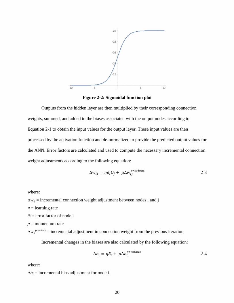
2 and is displayed graphically in Figure 2-2.

𝑂𝑗 = 𝑓(𝐼𝑗) =1

1+𝑒−𝐼𝑗

2-2

where:

Oj = output at node j

f(Ij) = sigmoidal activation function

Ij = input value at for node j

20

Figure 2-2: Sigmoidal function plot

Outputs from the hidden layer are then multiplied by their corresponding connection

weights, summed, and added to the biases associated with the output nodes according to

Equation 2-1 to obtain the input values for the output layer. These input values are then

processed by the activation function and de-normalized to provide the predicted output values for

the ANN. Error factors are calculated and used to compute the necessary incremental connection

weight adjustments according to the following equation:

∆𝑤𝑖𝑗 = 𝜂𝛿𝑖𝑂𝑗 + 𝜇∆𝑤𝑖𝑗𝑝𝑟𝑒𝑣𝑖𝑜𝑢𝑠

2-3

where:

∆wij = incremental connection weight adjustment between nodes i and j

η = learning rate

δi = error factor of node i

μ = momentum rate

∆wijprevious = incremental adjustment in connection weight from the previous iteration

Incremental changes in the biases are also calculated by the following equation:

∆𝑏𝑖 = 𝜂𝛿𝑖 + 𝜇∆𝑏𝑖𝑝𝑟𝑒𝑣𝑖𝑜𝑢𝑠

2-4

where:

∆bi = incremental bias adjustment for node i

10 5 5 10

0.2

0.4

0.6

0.8

1.0

21

∆bi previous = incremental adjustment in bias from the previous iteration

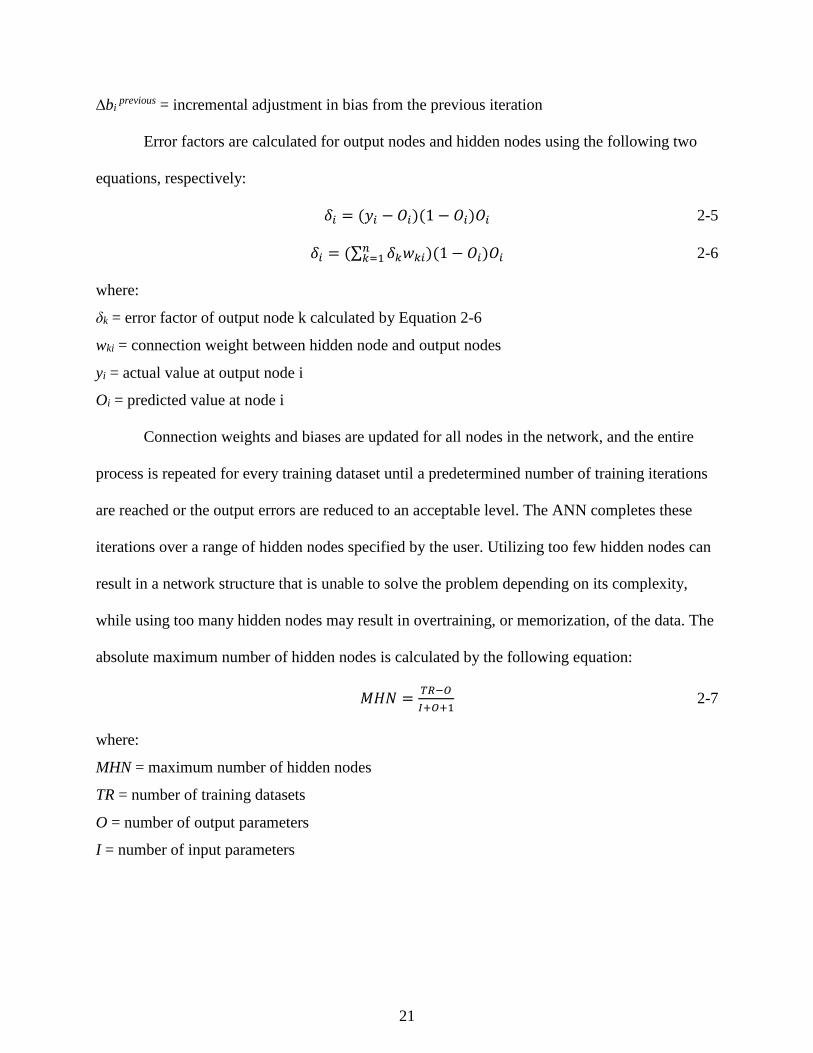
Error factors are calculated for output nodes and hidden nodes using the following two

equations, respectively:

𝛿𝑖 = (𝑦𝑖 − 𝑂𝑖)(1 − 𝑂𝑖)𝑂𝑖 2-5

𝛿𝑖 = (∑ 𝛿𝑘𝑤𝑘𝑖𝑛𝑘=1 )(1 − 𝑂𝑖)𝑂𝑖 2-6

where:

δk = error factor of output node k calculated by Equation 2-6

wki = connection weight between hidden node and output nodes

yi = actual value at output node i

Oi = predicted value at node i

Connection weights and biases are updated for all nodes in the network, and the entire

process is repeated for every training dataset until a predetermined number of training iterations

are reached or the output errors are reduced to an acceptable level. The ANN completes these

iterations over a range of hidden nodes specified by the user. Utilizing too few hidden nodes can

result in a network structure that is unable to solve the problem depending on its complexity,

while using too many hidden nodes may result in overtraining, or memorization, of the data. The

absolute maximum number of hidden nodes is calculated by the following equation:

𝑀𝐻𝑁 =𝑇𝑅−𝑂

𝐼+𝑂+1 2-7

where:

MHN = maximum number of hidden nodes

TR = number of training datasets

O = number of output parameters

I = number of input parameters

22

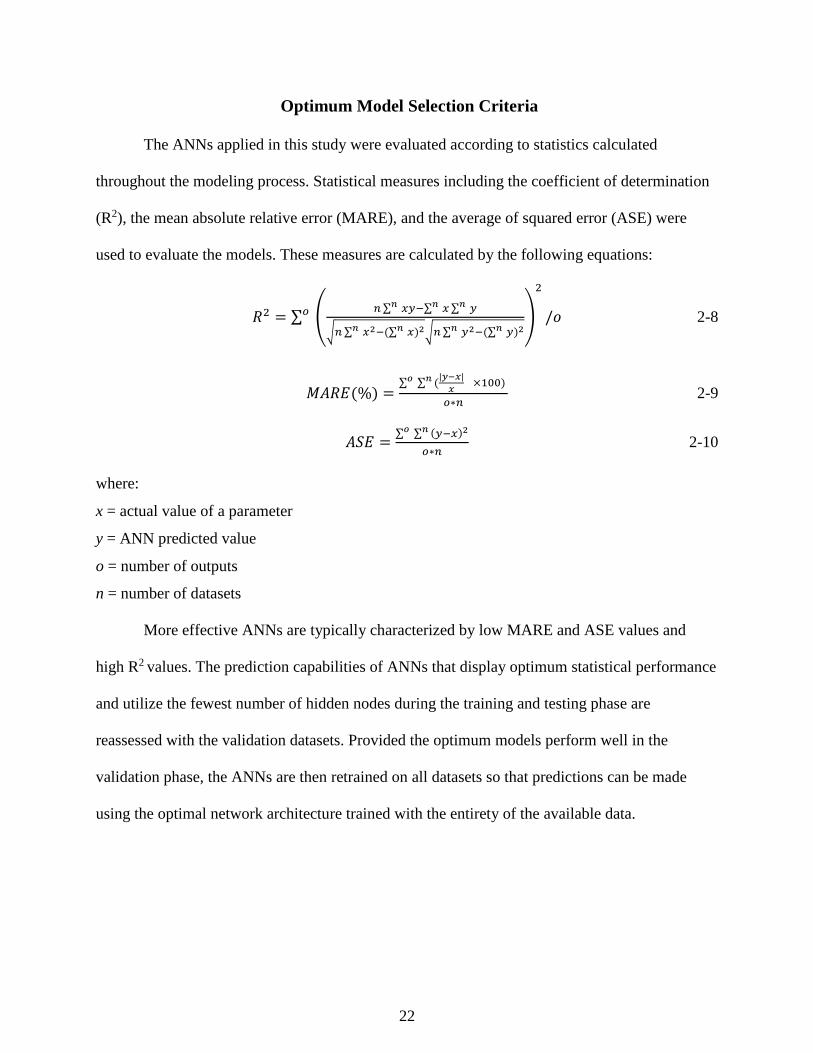
Optimum Model Selection Criteria

The ANNs applied in this study were evaluated according to statistics calculated

throughout the modeling process. Statistical measures including the coefficient of determination

(R2), the mean absolute relative error (MARE), and the average of squared error (ASE) were

used to evaluate the models. These measures are calculated by the following equations:

𝑅2 = ∑ (𝑛 ∑ 𝑥𝑦𝑛 −∑ 𝑥𝑛 ∑ 𝑦𝑛

√𝑛 ∑ 𝑥2𝑛 −(∑ 𝑥)2𝑛 √𝑛 ∑ 𝑦2𝑛 −(∑ 𝑦)2𝑛)

2

/𝑜𝑜 2-8

𝑀𝐴𝑅𝐸(%) =∑ ∑ (

|𝑦−𝑥|

𝑥𝑛 ×100) 𝑜

𝑜∗𝑛 2-9

𝐴𝑆𝐸 =∑ ∑ (𝑦−𝑥)2𝑛𝑜

𝑜∗𝑛 2-10

where:

x = actual value of a parameter

y = ANN predicted value

o = number of outputs

n = number of datasets

More effective ANNs are typically characterized by low MARE and ASE values and

high R2 values. The prediction capabilities of ANNs that display optimum statistical performance

and utilize the fewest number of hidden nodes during the training and testing phase are

reassessed with the validation datasets. Provided the optimum models perform well in the

validation phase, the ANNs are then retrained on all datasets so that predictions can be made

using the optimal network architecture trained with the entirety of the available data.

23

Chapter 3 - Methodology

The research project presented in this thesis is a continuation and expansion of the

damage evaluation component of Al Rahmani’s M.S. thesis (2012). The work in this study took

place over two primary phases: establishment of a reinforced concrete beam database using the

finite element (FE) method, and application of artificial neural networks (ANNs) to develop

damage evaluation, or structural health prediction models.

Generation of Reinforced Concrete Beam Database

Consistent with Al-Rahmani’s work (2012), reinforced concrete beams were modeled

using the FE analysis software program Abaqus, version 6.13 (Dassault Systèmes Simulia Corp.,

2013). However, Al-Rahmani’s study (2012) was restricted to FE analysis of rectangular sections

composed of two-dimensional (2D) plane stress elements with up to two cracks. It was desired

that the FE models in this research represent concrete T-beams reinforced with mild steel bars in

order to accurately emulate real-world bridge girders. Although all beams modeled in this study

were simply-supported, future work can apply the processes described in this chapter to beams

with any boundary condition configurations. Because construction and analysis of three-

dimensional (3D) FE models requires a significant amount of time and computational processing

power, the potential for using 2D reinforced concrete beams was first investigated. 2D planar

shell parts with thicknesses equal to the beam widths were used to model both the concrete beam

and steel reinforcement. Although rectangular beams were initially analyzed, T-beams were later

modeled by partitioning the concrete beams so that the thicknesses and widths of the flanges

could vary from those of the webs. The FE mesh applied to the beams and reinforcement

consisted of 8-node quadratic (CPS8) and 6-node triangular (CPS6) plane stress elements. To

provide a standard against which the performance of the 2D beam models could be measured, 3D

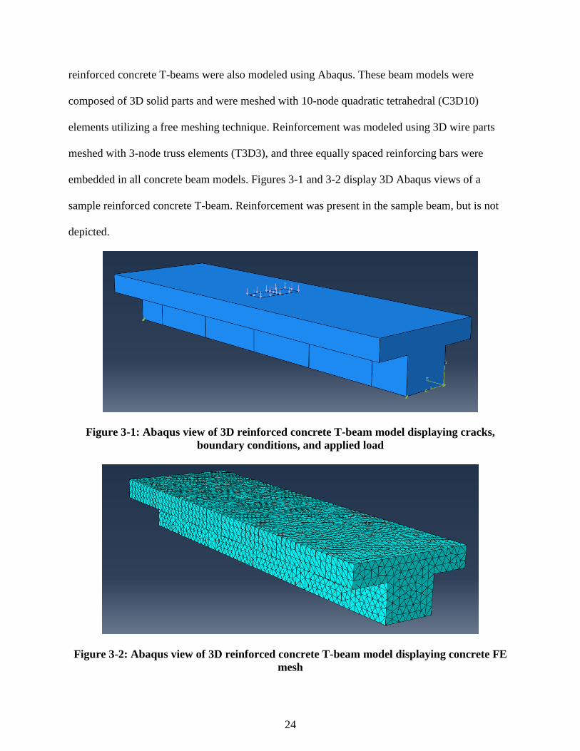
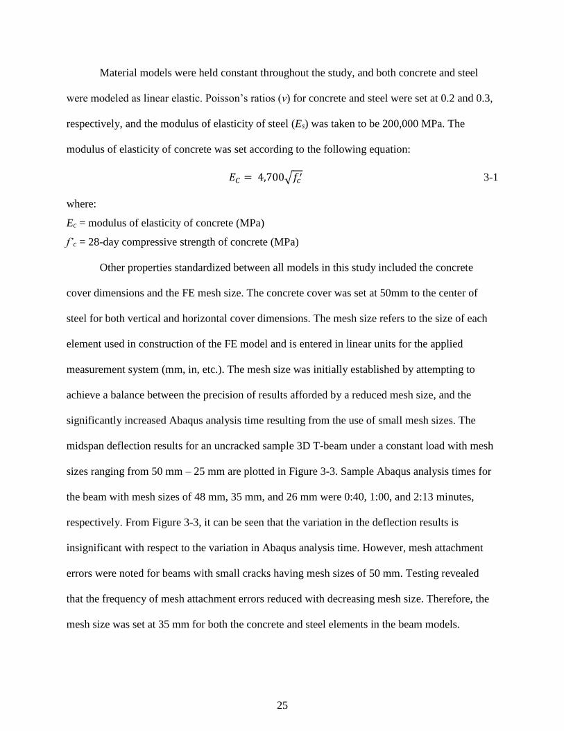
24

reinforced concrete T-beams were also modeled using Abaqus. These beam models were

composed of 3D solid parts and were meshed with 10-node quadratic tetrahedral (C3D10)

elements utilizing a free meshing technique. Reinforcement was modeled using 3D wire parts

meshed with 3-node truss elements (T3D3), and three equally spaced reinforcing bars were

embedded in all concrete beam models. Figures 3-1 and 3-2 display 3D Abaqus views of a

sample reinforced concrete T-beam. Reinforcement was present in the sample beam, but is not

depicted.

Figure 3-1: Abaqus view of 3D reinforced concrete T-beam model displaying cracks,

boundary conditions, and applied load

Figure 3-2: Abaqus view of 3D reinforced concrete T-beam model displaying concrete FE

mesh

25

Material models were held constant throughout the study, and both concrete and steel

were modeled as linear elastic. Poisson’s ratios (ν) for concrete and steel were set at 0.2 and 0.3,

respectively, and the modulus of elasticity of steel (Es) was taken to be 200,000 MPa. The

modulus of elasticity of concrete was set according to the following equation:

𝐸𝐶 = 4,700√𝑓𝑐′ 3-1

where:

Ec = modulus of elasticity of concrete (MPa)

f’c = 28-day compressive strength of concrete (MPa)

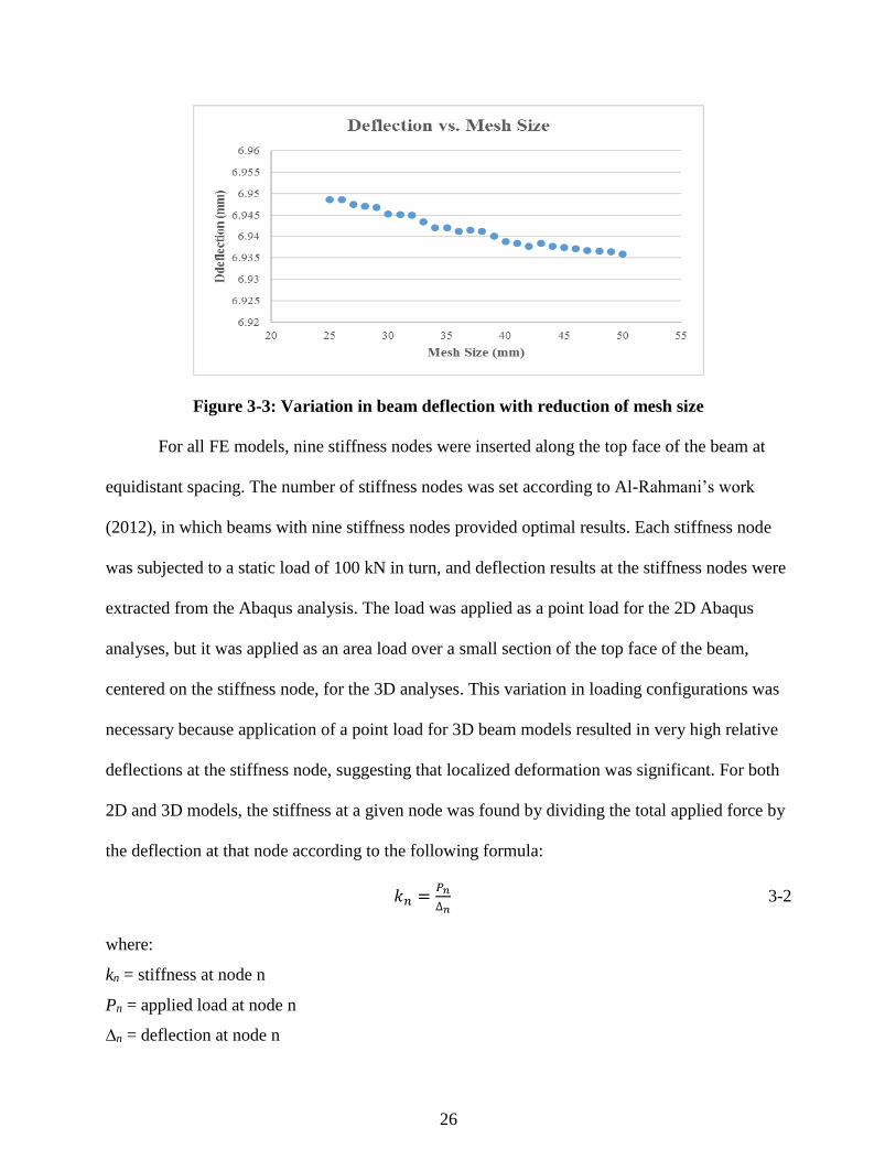
Other properties standardized between all models in this study included the concrete

cover dimensions and the FE mesh size. The concrete cover was set at 50mm to the center of

steel for both vertical and horizontal cover dimensions. The mesh size refers to the size of each

element used in construction of the FE model and is entered in linear units for the applied

measurement system (mm, in, etc.). The mesh size was initially established by attempting to

achieve a balance between the precision of results afforded by a reduced mesh size, and the

significantly increased Abaqus analysis time resulting from the use of small mesh sizes. The

midspan deflection results for an uncracked sample 3D T-beam under a constant load with mesh

sizes ranging from 50 mm – 25 mm are plotted in Figure 3-3. Sample Abaqus analysis times for

the beam with mesh sizes of 48 mm, 35 mm, and 26 mm were 0:40, 1:00, and 2:13 minutes,

respectively. From Figure 3-3, it can be seen that the variation in the deflection results is

insignificant with respect to the variation in Abaqus analysis time. However, mesh attachment

errors were noted for beams with small cracks having mesh sizes of 50 mm. Testing revealed

that the frequency of mesh attachment errors reduced with decreasing mesh size. Therefore, the

mesh size was set at 35 mm for both the concrete and steel elements in the beam models.

26

Figure 3-3: Variation in beam deflection with reduction of mesh size

For all FE models, nine stiffness nodes were inserted along the top face of the beam at

equidistant spacing. The number of stiffness nodes was set according to Al-Rahmani’s work

(2012), in which beams with nine stiffness nodes provided optimal results. Each stiffness node

was subjected to a static load of 100 kN in turn, and deflection results at the stiffness nodes were

extracted from the Abaqus analysis. The load was applied as a point load for the 2D Abaqus

analyses, but it was applied as an area load over a small section of the top face of the beam,

centered on the stiffness node, for the 3D analyses. This variation in loading configurations was

necessary because application of a point load for 3D beam models resulted in very high relative

deflections at the stiffness node, suggesting that localized deformation was significant. For both

2D and 3D models, the stiffness at a given node was found by dividing the total applied force by

the deflection at that node according to the following formula:

𝑘𝑛 =𝑃𝑛

∆𝑛 3-2

where:

kn = stiffness at node n

Pn = applied load at node n

∆n = deflection at node n

27

Nodal stiffnesses were obtained for uncracked, or healthy, and cracked beams. Cracked

beams were modeled with discontinuities corresponding to the crack depth and width for 2D

beam models, and as extruded cuts in the beam web for 3D models. Only vertical flexural cracks

were considered in this study. The damage level in cracked beams was determined quantitatively

by calculating the stiffness ratio at each node, which was defined as the cracked stiffness divided

by the healthy stiffness of beams with identical geometries and material properties. Nodal

stiffness ratios were computed according to the following equation:

𝑘%𝑛 =𝑘𝑛,𝑐𝑟

𝑘𝑛,ℎ 3-3

where:

k%n = stiffness ratio at node n

kn,cr = stiffness at node n of a cracked beam

kn,h = stiffness at node n of a healthy beam

Nodal stiffness ratios were used to quantitatively describe the damage level, or residual

structural health, of the reinforced concrete beams. In general, beams with low nodal stiffness

ratios have deep, wide, or an extensive number of cracks. Nodal stiffness ratios were also found

to indicate damage locations within a beam; stiffness ratios of nodes near existing cracks are

typically lower than stiffness ratios of nodes far from damage locations. It was observed that

cracks placed very close to the beam supports resulted in unreasonably low nodal stiffness ratios.

This was thought to be due in part to a failure to meet Saint-Venant’s principle, which suggests

that the stress distribution in a material may be assumed to be independent of the manner of load

application, except in the immediate vicinity of the applied loads (Beer, Johnston, Dewolf, &

Mazurek, 2012). The presence of both an applied load and a discontinuity (crack) in the beam

close to the supports likely introduced stress and strain concentrations that contributed to the

deflection of the beam. Therefore, crack placement was limited to 0.06–0.94 of the beam span

28

length; a range in which the nodal stiffness ratios were generally observed to stabilize to

reasonable values.

Several healthy and cracked test beams were created with consistent geometric and

material properties between the 2D rectangular beam, 2D T-beam, and 3D T-beam models.

Stiffness ratios of these test beams were compared between the three Abaqus model types.

Establishment of an equivalency between stiffness ratio results of the 2D rectangular beams and

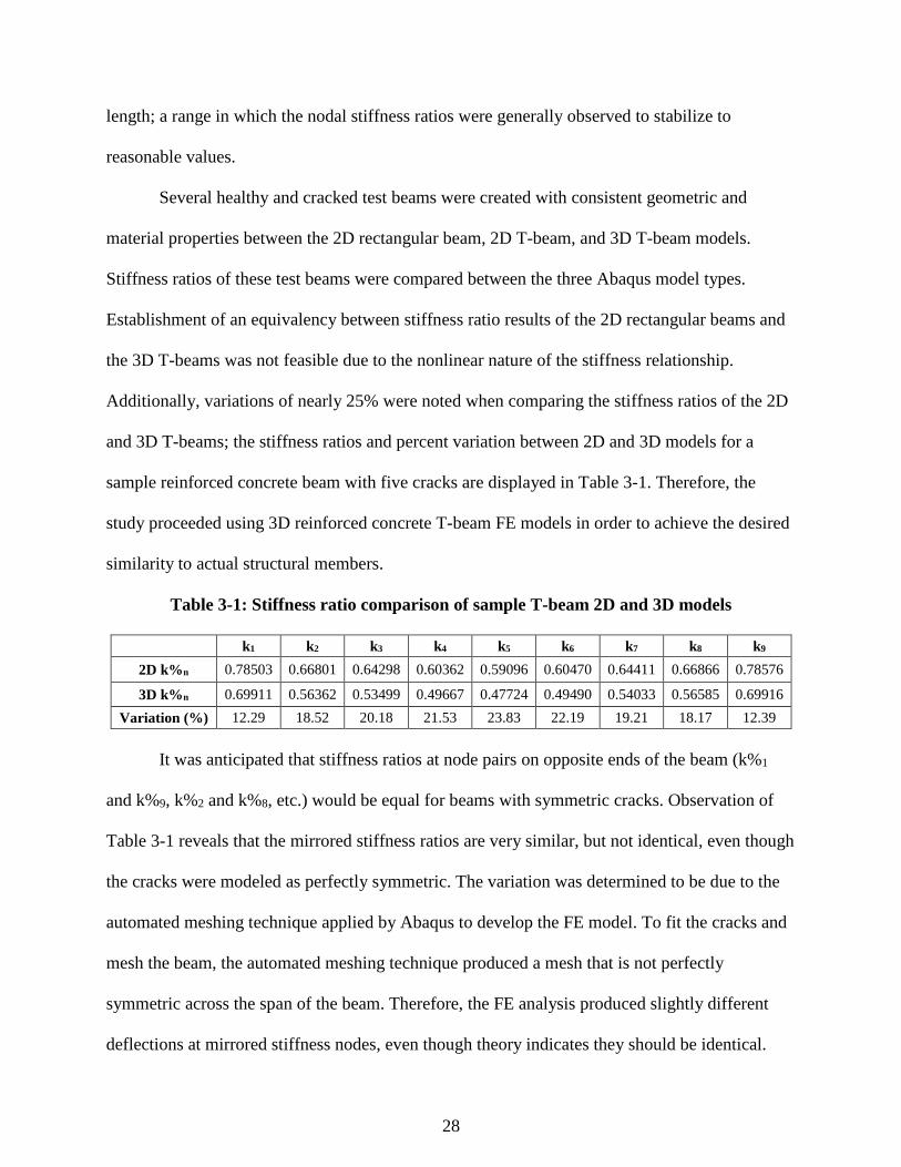
the 3D T-beams was not feasible due to the nonlinear nature of the stiffness relationship.

Additionally, variations of nearly 25% were noted when comparing the stiffness ratios of the 2D

and 3D T-beams; the stiffness ratios and percent variation between 2D and 3D models for a

sample reinforced concrete beam with five cracks are displayed in Table 3-1. Therefore, the

study proceeded using 3D reinforced concrete T-beam FE models in order to achieve the desired

similarity to actual structural members.

Table 3-1: Stiffness ratio comparison of sample T-beam 2D and 3D models

k1 k2 k3 k4 k5 k6 k7 k8 k9

2D k%n 0.78503 0.66801 0.64298 0.60362 0.59096 0.60470 0.64411 0.66866 0.78576

3D k%n 0.69911 0.56362 0.53499 0.49667 0.47724 0.49490 0.54033 0.56585 0.69916

Variation (%) 12.29 18.52 20.18 21.53 23.83 22.19 19.21 18.17 12.39

It was anticipated that stiffness ratios at node pairs on opposite ends of the beam (k%1

and k%9, k%2 and k%8, etc.) would be equal for beams with symmetric cracks. Observation of

Table 3-1 reveals that the mirrored stiffness ratios are very similar, but not identical, even though

the cracks were modeled as perfectly symmetric. The variation was determined to be due to the

automated meshing technique applied by Abaqus to develop the FE model. To fit the cracks and

mesh the beam, the automated meshing technique produced a mesh that is not perfectly

symmetric across the span of the beam. Therefore, the FE analysis produced slightly different

deflections at mirrored stiffness nodes, even though theory indicates they should be identical.

29

The 3D reinforced concrete T-beam database was established by variation of the

geometric and material parameters for all beams as well as cracking parameters for cracked

beams. Geometric parameters included the width of the beam web cross-section (bw), the depth

of the entire beam cross-section (h), the height of the beam flange, or slab (hs), and the beam

span length (L). The beam flange was modeled according to the provisions of American

Concrete Institute (ACI) 318-14 Section 8.4.1.8 for two-way slabs, which indicates that the total

width of the T-beam flange should be equal to the sum of the web width and twice the depth of

the beam extending below the flange as shown in Figure 3-4 (ACI Committee 318, 2014).

Figure 3-4: T-beam flange dimensions

The size of the reinforcing bars in each beam depended upon the steel ratio (ρ) and the

beam’s cross-sectional area according to the relationship As = ρbwd, where As is the total cross-

sectional area of steel reinforcement and d is the effective depth of the beam section, taken as the

beam depth minus the cover. The 28-day concrete compressive strength (f’c) was the only

variable material parameter. Cracking parameters included the location (bcr), depth (dcr), and

width (wcr) of each crack, and all crack locations were measured from a constant (left) edge of

the beam. With the exception of f’c, ρ, and wcr, all parameters were directly normalized with

respect to a beam web width of bw = 250 mm, resulting in the normalized parameters bw/h, hs/h,

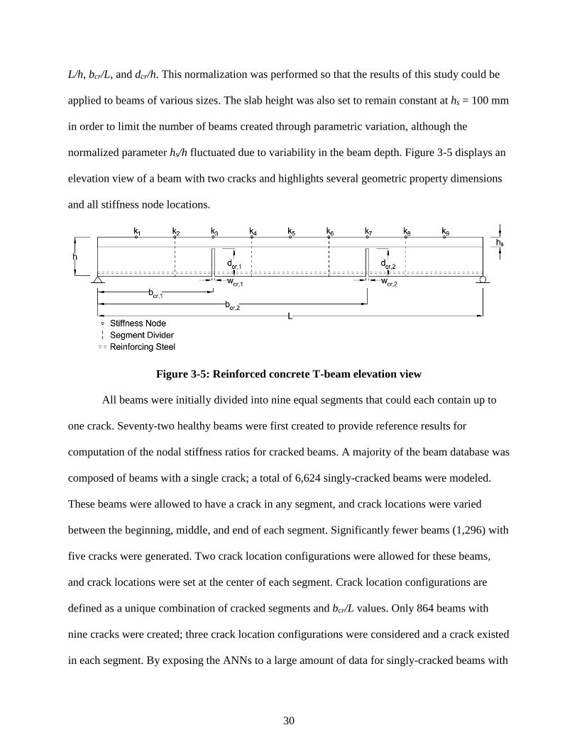
30

L/h, bcr/L, and dcr/h. This normalization was performed so that the results of this study could be

applied to beams of various sizes. The slab height was also set to remain constant at hs = 100 mm

in order to limit the number of beams created through parametric variation, although the

normalized parameter hs/h fluctuated due to variability in the beam depth. Figure 3-5 displays an

elevation view of a beam with two cracks and highlights several geometric property dimensions

and all stiffness node locations.

Figure 3-5: Reinforced concrete T-beam elevation view

All beams were initially divided into nine equal segments that could each contain up to

one crack. Seventy-two healthy beams were first created to provide reference results for

computation of the nodal stiffness ratios for cracked beams. A majority of the beam database was

composed of beams with a single crack; a total of 6,624 singly-cracked beams were modeled.

These beams were allowed to have a crack in any segment, and crack locations were varied

between the beginning, middle, and end of each segment. Significantly fewer beams (1,296) with

five cracks were generated. Two crack location configurations were allowed for these beams,

and crack locations were set at the center of each segment. Crack location configurations are

defined as a unique combination of cracked segments and bcr/L values. Only 864 beams with

nine cracks were created; three crack location configurations were considered and a crack existed

in each segment. By exposing the ANNs to a large amount of data for singly-cracked beams with

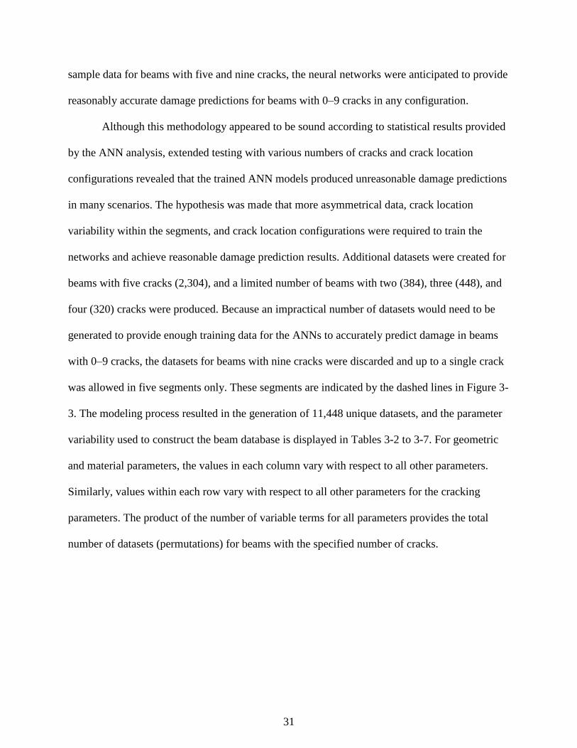
31

sample data for beams with five and nine cracks, the neural networks were anticipated to provide

reasonably accurate damage predictions for beams with 0–9 cracks in any configuration.

Although this methodology appeared to be sound according to statistical results provided

by the ANN analysis, extended testing with various numbers of cracks and crack location

configurations revealed that the trained ANN models produced unreasonable damage predictions

in many scenarios. The hypothesis was made that more asymmetrical data, crack location

variability within the segments, and crack location configurations were required to train the

networks and achieve reasonable damage prediction results. Additional datasets were created for

beams with five cracks (2,304), and a limited number of beams with two (384), three (448), and

four (320) cracks were produced. Because an impractical number of datasets would need to be

generated to provide enough training data for the ANNs to accurately predict damage in beams

with 0–9 cracks, the datasets for beams with nine cracks were discarded and up to a single crack

was allowed in five segments only. These segments are indicated by the dashed lines in Figure 3-

3. The modeling process resulted in the generation of 11,448 unique datasets, and the parameter

variability used to construct the beam database is displayed in Tables 3-2 to 3-7. For geometric

and material parameters, the values in each column vary with respect to all other parameters.

Similarly, values within each row vary with respect to all other parameters for the cracking

parameters. The product of the number of variable terms for all parameters provides the total

number of datasets (permutations) for beams with the specified number of cracks.

32

Table 3-2: Parameter variability for singly-cracked beams

Parameters Values Variable Terms

bw/h 0.5 0.7 0.9 3

L/h 7 10 13 3

ρ 0.005 0.01 2

f'c (MPa) 20 30 40 50 4

Segment 1 Segment 2 Segment 3 Segment 4 Segment 5

bcr/L

0.06

23

0.1

0.15

0.2

0.2

0.25

0.3

0.35

0.4

0.4

0.45

0.5

0.55

0.6

0.6

0.65

0.7

0.75

0.8

0.8

0.85

0.9

0.94

Crack 1

dcr/h 0.25

2 0.64

wcr (mm) 1

2 5

Number of Beam Datasets = 6624

* bw = 250 mm and hs = 100 mm

33

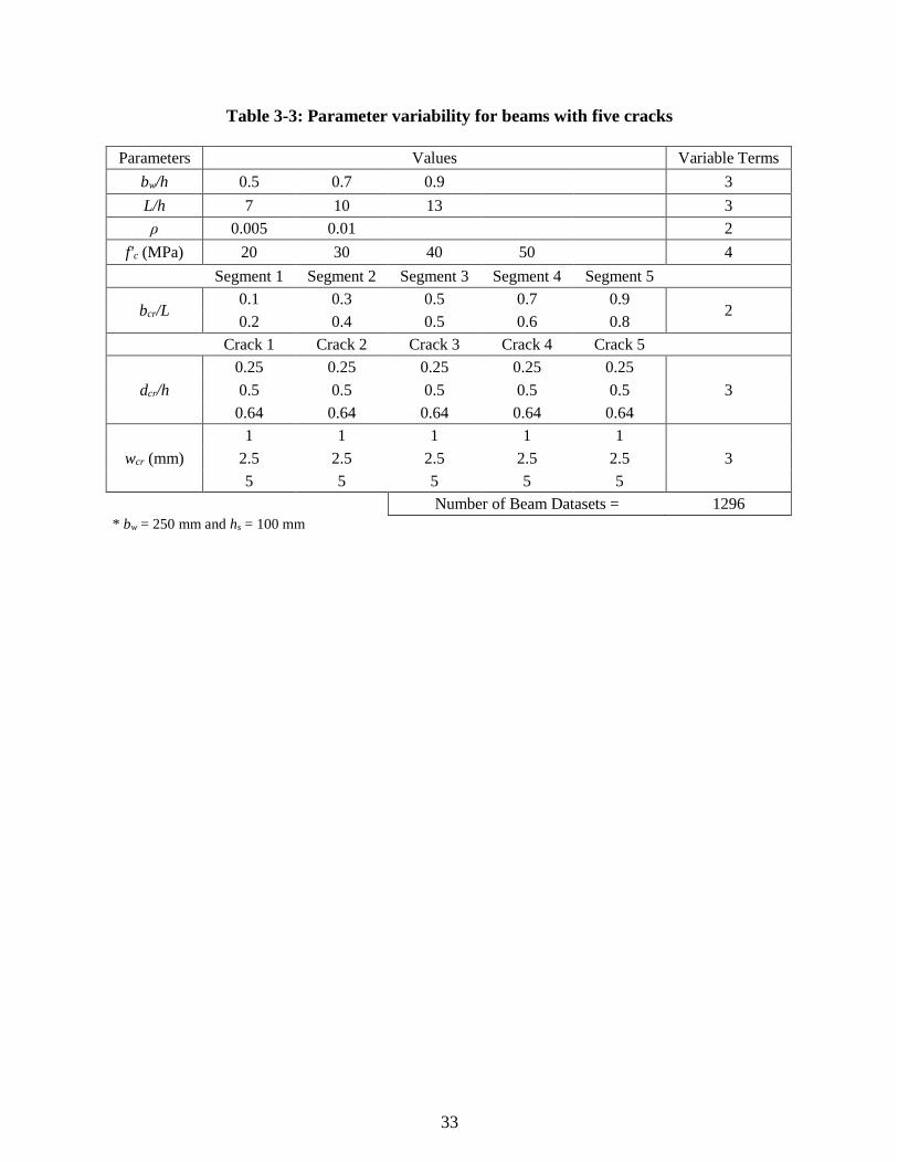
Table 3-3: Parameter variability for beams with five cracks

Parameters Values Variable Terms

bw/h 0.5 0.7 0.9 3

L/h 7 10 13 3

ρ 0.005 0.01 2

f'c (MPa) 20 30 40 50 4

Segment 1 Segment 2 Segment 3 Segment 4 Segment 5

bcr/L 0.1 0.3 0.5 0.7 0.9

2 0.2 0.4 0.5 0.6 0.8

Crack 1 Crack 2 Crack 3 Crack 4 Crack 5

dcr/h

0.25 0.25 0.25 0.25 0.25

3 0.5 0.5 0.5 0.5 0.5

0.64 0.64 0.64 0.64 0.64

wcr (mm)

1 1 1 1 1

3 2.5 2.5 2.5 2.5 2.5

5 5 5 5 5

Number of Beam Datasets = 1296

* bw = 250 mm and hs = 100 mm

34

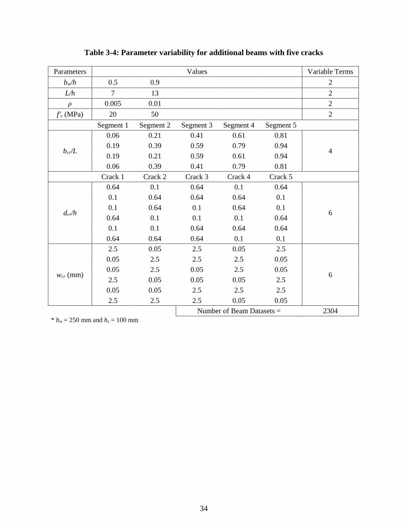
Table 3-4: Parameter variability for additional beams with five cracks

Parameters Values Variable Terms

bw/h 0.5 0.9 2

L/h 7 13 2

ρ 0.005 0.01 2

f'c (MPa) 20 50 2

Segment 1 Segment 2 Segment 3 Segment 4 Segment 5

bcr/L

0.06 0.21 0.41 0.61 0.81

4 0.19 0.39 0.59 0.79 0.94

0.19 0.21 0.59 0.61 0.94

0.06 0.39 0.41 0.79 0.81

Crack 1 Crack 2 Crack 3 Crack 4 Crack 5

dcr/h

0.64 0.1 0.64 0.1 0.64

6

0.1 0.64 0.64 0.64 0.1

0.1 0.64 0.1 0.64 0.1

0.64 0.1 0.1 0.1 0.64

0.1 0.1 0.64 0.64 0.64

0.64 0.64 0.64 0.1 0.1

wcr (mm)

2.5 0.05 2.5 0.05 2.5

6

0.05 2.5 2.5 2.5 0.05

0.05 2.5 0.05 2.5 0.05

2.5 0.05 0.05 0.05 2.5

0.05 0.05 2.5 2.5 2.5

2.5 2.5 2.5 0.05 0.05

Number of Beam Datasets = 2304

* bw = 250 mm and hs = 100 mm

35

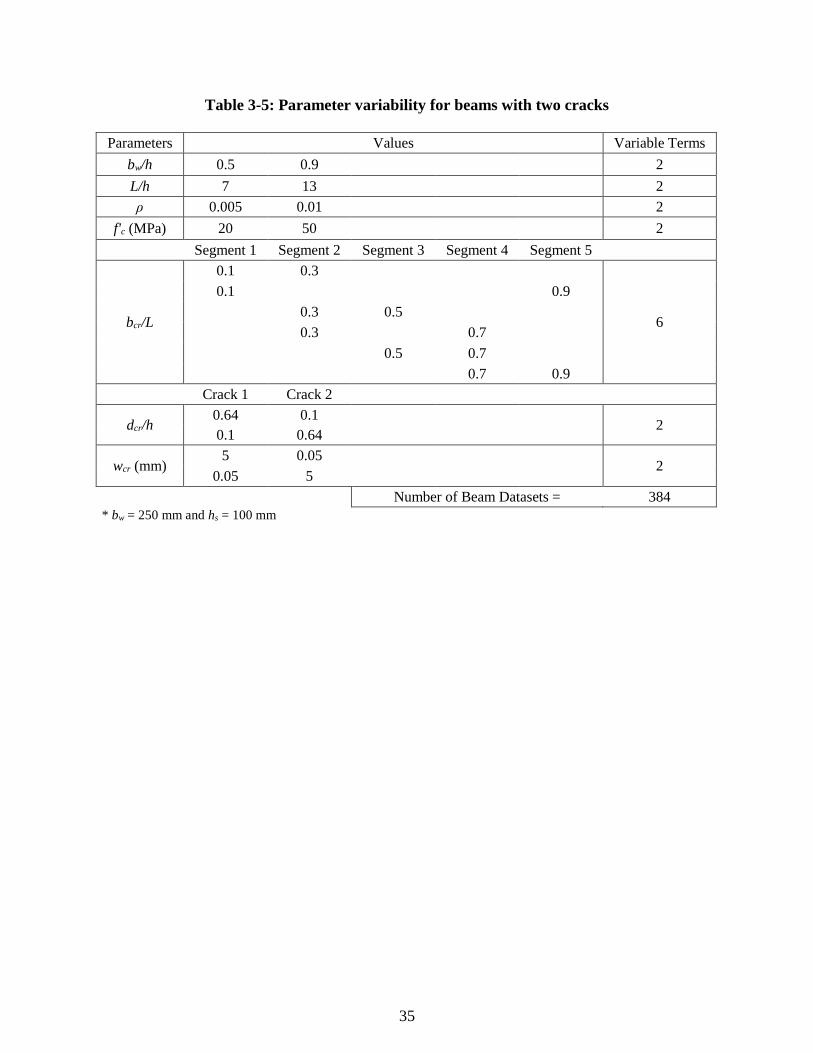
Table 3-5: Parameter variability for beams with two cracks

Parameters Values Variable Terms

bw/h 0.5 0.9 2

L/h 7 13 2

ρ 0.005 0.01 2

f'c (MPa) 20 50 2

Segment 1 Segment 2 Segment 3 Segment 4 Segment 5

bcr/L

0.1 0.3

6

0.1 0.9

0.3 0.5

0.3 0.7

0.5 0.7

0.7 0.9

Crack 1 Crack 2

dcr/h 0.64 0.1

2 0.1 0.64

wcr (mm) 5 0.05

2 0.05 5

Number of Beam Datasets = 384

* bw = 250 mm and hs = 100 mm

36

Table 3-6: Parameter variability for beams with three cracks

Parameters Values Variable Terms

bw/h 0.5 0.9 2

L/h 7 13 2

ρ 0.005 0.01 2

f'c (MPa) 20 50 2

Segment 1 Segment 2 Segment 3 Segment 4 Segment 5

bcr/L

0.1 0.5 0.9

7

0.1 0.7 0.9

0.1 0.3 0.5

0.1 0.3 0.7

0.1 0.3 0.9

0.3 0.7 0.9

0.5 0.7 0.9

Crack 1 Crack 2 Crack 3

dcr/h 0.64 0.25 0.1

2 0.1 0.25 0.64

wcr (mm) 5 2.5 0.05

2 0.05 2.5 5

Number of Beam Datasets = 448

* bw = 250 mm and hs = 100 mm

37

Table 3-7: Parameter variability for beams with four cracks

Parameters Values Variable Terms

bw/h 0.5 0.9 2

L/h 7 13 2

ρ 0.005 0.01 2

f'c (MPa) 20 50 2

Segment 1 Segment 2 Segment 3 Segment 4 Segment 5

bcr/L

0.1 0.3 0.5 0.7

5

0.1 0.3 0.5 0.9

0.1 0.3 0.7 0.9

0.1 0.5 0.7 0.9

0.3 0.5 0.7 0.9

Crack 1 Crack 2 Crack 3 Crack 4

dcr/h 0.64 0.25 0.64 0.1

2 0.1 0.64 0.25 0.64

wcr (mm) 5 2.5 5 0.05

2 0.05 5 2.5 5

Number of Beam Datasets = 320

* bw = 250 mm and hs = 100 mm

Segments absent of cracks were initially assigned bcr/L, dcr/h, and wcr values of zero.

However, Dr. Najjar advised that the ANNs would require the crack locations to be nonzero in

order to establish adequate prediction logic (Y. Najjar, personal communication, December 11,

2015). Therefore, bcr/L values were set at the center of each segment for all segments with no

crack present, while dcr/h and wcr values were maintained at zero. The possibility of expanding

the database without generating additional FE models was noted, and datasets for the healthy

beams and beams with one, two, three, and four cracks were duplicated according to the four

crack location configurations shown in Table 3-4. Segments without cracks for these beams were

assigned bcr/L values corresponding to these four crack location configurations. For example, a

beam with a single crack at midspan would first be assigned bcr/L values of 0.1, 0.3, 0.5, 0.7, and

0.9 in segments 1, 2, 3, 4, and 5, respectively. This beam would then be duplicated by copying

all parameters and changing the bcr/L values for all segments without cracks, or segments 1, 2, 4,

38

and 5, to 0.06, 0.21, 0.61, and 0.81, respectively. These values correspond to the bcr/L values for

the first crack location configuration in Table 3-4. The beam could be duplicated three more

times according to the three remaining crack location configurations. This duplication procedure

would result in five beams with identical geometric, material, and cracking parameters (with the

exception of crack locations in segments devoid of cracks), as well as identical nodal stiffness

ratios and health indices. Using this methodology, the beam database was expanded from 11,448

datasets to 42,840 datasets. As advised by Dr. Najjar, all duplicated datasets were applied as

training sets in ANN analyses.

Abaqus macros were recorded as Python scripts for the creation of healthy beams and

beams with one, two, three, four, and five cracks. These scripts were adapted according to Al-

Rahmani’s work (2012) and were used to automate the generation of input files (.inp files) for

3D models through the Abaqus user interface. A Python script provided by Al-Rahmani allowed

automated analysis of input files by directly interfacing with Abaqus, and a final script extracted

the resultant nodal deflections from the Abaqus binary output databases (.odb files). These

deflections were used to determine the nodal stiffness ratios, as previously described. Example

generation, analysis, and extraction scripts are contained in Appendix A.

To verify that the results of this approach would be applicable to a range of typical girder

sizes, 50 cracked beams were selected at random from the 11,448 unique datasets. All geometric,

material, and cracking parameters for these beams were held constant with the exception of the

web width, and additional healthy and cracked beams were modeled with these parameters for

web widths of 200 mm and 300 mm. The hs/h normalized parameter remained constant for these

additional models, causing the height of the slab to be 80 mm and 120 mm for all beams with

web widths of 200 mm and 300 mm, respectively. After the FE models were analyzed and nodal

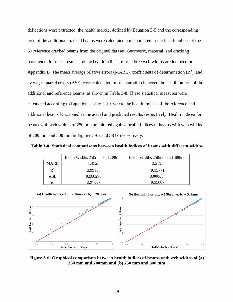
39

deflections were extracted, the health indices, defined by Equation 3-5 and the corresponding

text, of the additional cracked beams were calculated and compared to the health indices of the

50 reference cracked beams from the original dataset. Geometric, material, and cracking

parameters for these beams and the health indices for the three web widths are included in

Appendix B. The mean average relative errors (MARE), coefficients of determination (R2), and

average squared errors (ASE) were calculated for the variation between the health indices of the

additional and reference beams, as shown in Table 3-8. These statistical measures were

calculated according to Equations 2-8 to 2-10, where the health indices of the reference and

additional beams functioned as the actual and predicted results, respectively. Health indices for

beams with web widths of 250 mm are plotted against health indices of beams with web widths

of 200 mm and 300 mm in Figures 3-6a and 3-6b, respectively.

Table 3-8: Statistical comparisons between health indices of beams with different widths

Beam Widths 250mm and 200mm Beam Widths 250mm and 300mm

MARE 1.4525 0.5198

R2 0.99103 0.99771

ASE 0.000295 0.000034

ρc 0.97667 0.99687

Figure 3-6: Graphical comparison between health indices of beams with web widths of (a)

250 mm and 200mm and (b) 250 mm and 300 mm

40

The low errors and high coefficients of determination evident in Table 3-8 indicate good

agreement between the health index results of beams with different web widths. As shown in

Figure 3-6, the health indices of large beams (bw = 300 mm) are more similar to the health

indices of the reference beams than are the health indices of small beams (bw = 200 mm). A brief

sensitivity analysis, performed by reducing the mesh size from 35 mm to 25 mm for the small

beams, resulted in similar health indices and revealed that mesh coarseness did not substantially

affect the results. It was therefore hypothesized that the relationship between the beam size and

the stiffness provided by the FE model mesh is nonlinear and cracking damage affects the

structural health of small beams significantly more than large beams. In addition to the MARE,

R2, and ASE results, Lin’s concordance correlation coefficient values (ρc) are displayed in Table

3-8. Lin’s concordance correlation coefficient, defined by Equation 3-4, serves as a

reproducibility index by which the quality of new measurements can be judged, and ranges

between 0 for poor correlation and 1 for perfect correlation (Lin, 1989). This coefficient assesses

how well the damage results for beams with web widths of 250 mm can be applied to beams with

web widths ranging from 200 mm to 300 mm. Lin’s concordance correlation coefficients

exceeded 0.975 for both comparisons. The high value of this coefficient, in addition to the

favorable results of the other three statistical measures, indicated that the results of this study can

be applied to a variety of typical girder sizes.

𝜌𝑐 =2𝜌 𝜎𝑟𝜎𝑡

𝜎𝑟2+𝜎𝑡

2+(𝜇𝑟−𝜇𝑡)2 3-4

where:

ρ = square root of R2, or Pearson correlation coefficient between the reference and test data

σr = square root of the variance, or standard deviation, of the reference data

σt = square root of the variance, or standard deviations of the test data

μr = mean of the reference data

μr = mean of the test data

41

ANN Modeling for Structural Health Prediction

Two ANNs were trained in order to develop structural health prediction models for

reinforced concrete T-beams. The first network was trained with the geometric, material, and

cracking parameters (bw/h, hs/h, L/h, ρ, f’c, bcr,m/L, dcr,m/h, and wcr,m, where m denotes the mth

crack) as inputs and the stiffness ratios (k%n, where n is the nth stiffness node) at the nine

equidistant stiffness nodes as outputs. Because solving for nine different outputs given 20 input

parameters presents a highly complex problem, the second ANN was trained with the same input

parameters, but only one output parameter: the health index (ki%). Referencing Al-Rahmani’s

work (2012), the health index was calculated by integrating the area under the stiffness ratio

profile over the beam span length. This relationship is displayed in Figure 3-7 where the health

index is taken approximately as the hatched area under the stiffness ratio profile for a sample

beam with five cracks. A quantifiable measure of damage was maintained by resolving the nodal

stiffness ratios into a single term, thereby simplifying the problem that the ANN was required to

solve. The health index is described by the following equation:

𝐻𝑒𝑎𝑙𝑡ℎ 𝐼𝑛𝑑𝑒𝑥 (𝑘𝑖%) = (𝑙𝑛

𝐿) (1 + ∑ 𝑘%𝑛

𝑛=9𝑛=1 ) 3-5

where:

ln = distance between two consecutive stiffness nodes

L = beam span length

k%n = stiffness ratio at node n

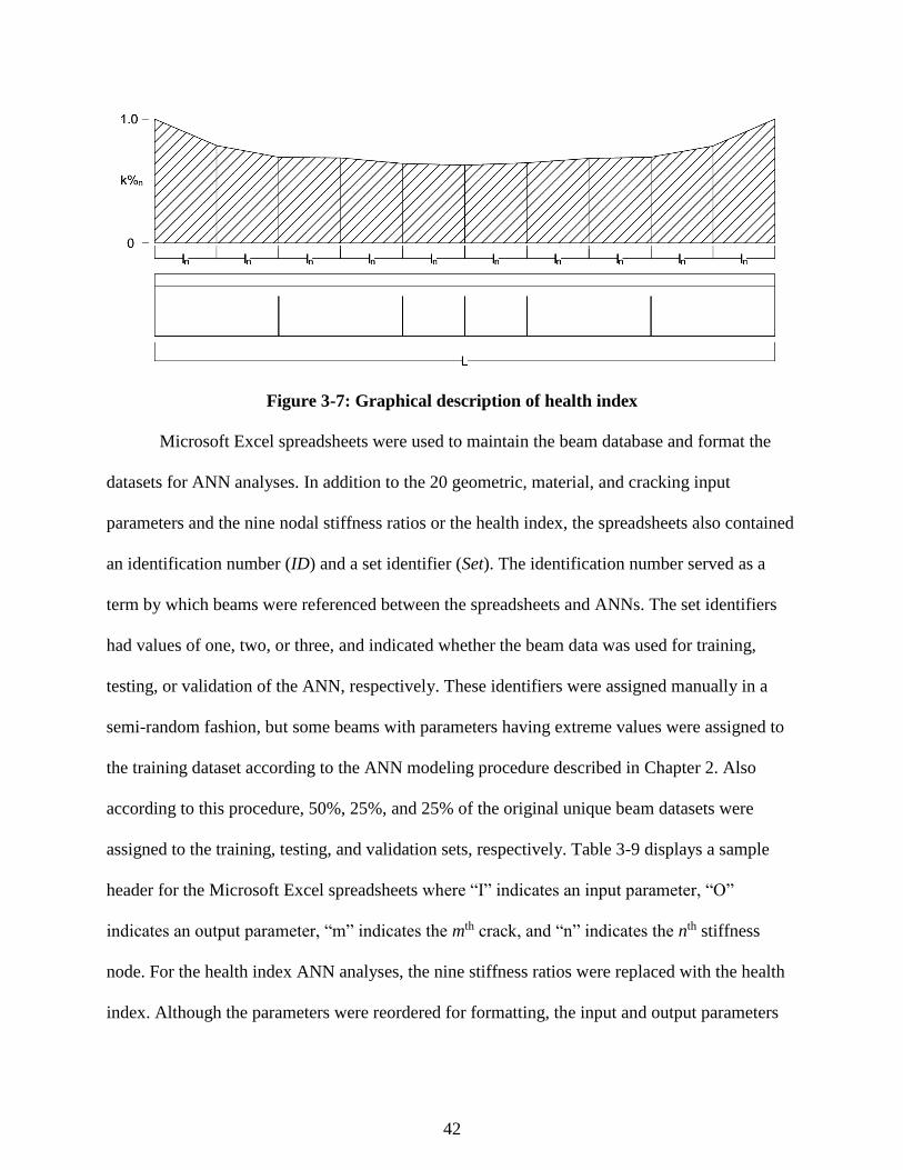
42

Figure 3-7: Graphical description of health index

Microsoft Excel spreadsheets were used to maintain the beam database and format the

datasets for ANN analyses. In addition to the 20 geometric, material, and cracking input

parameters and the nine nodal stiffness ratios or the health index, the spreadsheets also contained

an identification number (ID) and a set identifier (Set). The identification number served as a

term by which beams were referenced between the spreadsheets and ANNs. The set identifiers

had values of one, two, or three, and indicated whether the beam data was used for training,

testing, or validation of the ANN, respectively. These identifiers were assigned manually in a

semi-random fashion, but some beams with parameters having extreme values were assigned to

the training dataset according to the ANN modeling procedure described in Chapter 2. Also

according to this procedure, 50%, 25%, and 25% of the original unique beam datasets were

assigned to the training, testing, and validation sets, respectively. Table 3-9 displays a sample

header for the Microsoft Excel spreadsheets where “I” indicates an input parameter, “O”

indicates an output parameter, “m” indicates the mth crack, and “n” indicates the nth stiffness

node. For the health index ANN analyses, the nine stiffness ratios were replaced with the health

index. Although the parameters were reordered for formatting, the input and output parameters

43

for a sample of approximately 500 datasets from the unique beam database can are presented in

Appendix C.

Table 3-9: Sample Microsoft Excel database header

ID bw/h hs/h L/h ρ f'c (MPa) bcr,m/L dcr,m/h wcr,m (mm) k%n Set

# I I I I I I I I O 1, 2, or 3

Both the nodal stiffness ratio and health index prediction models were developed

according to the ANN modeling procedure described in Chapter 2. The final reinforced concrete

beam database contained data for 42,480 beams, and 37,116 (5,724 original and 31,392

duplicated), 2,862, and 2,862 beams were employed in training, testing, and validating the

ANNs, respectively. Minimum and maximum parameter value ranges supplied to the ANNs

were expanded to keep the actual parameter values in the sensitive region of the sigmoidal

activation function of the network. The input parameter range was expanded to allow the input

parameters to fit within 10%–90% of the expanded range. Nodal stiffness ratios and health

indices were limited to those of a healthy beam (<=1.0), so the output parameter range was

expanded so that only the minimum values were modified and the output parameters fit within

20%–100% of the expanded range. The expanded parameter ranges are displayed in Table 3-10.

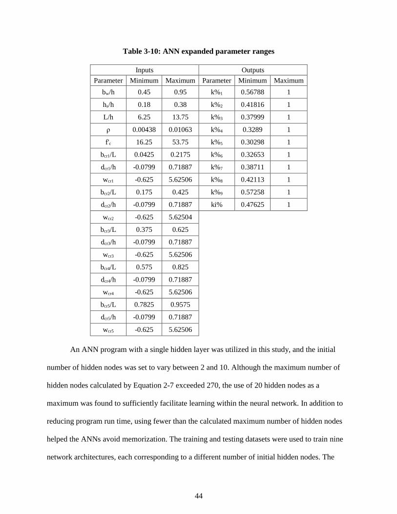
44

Table 3-10: ANN expanded parameter ranges

Inputs Outputs

Parameter Minimum Maximum Parameter Minimum Maximum

bw/h 0.45 0.95 k%1 0.56788 1

hs/h 0.18 0.38 k%2 0.41816 1

L/h 6.25 13.75 k%3 0.37999 1

ρ 0.00438 0.01063 k%4 0.3289 1

f'c 16.25 53.75 k%5 0.30298 1

bcr1/L 0.0425 0.2175 k%6 0.32653 1

dcr1/h -0.0799 0.71887 k%7 0.38711 1

wcr1 -0.625 5.62506 k%8 0.42113 1

bcr2/L 0.175 0.425 k%9 0.57258 1

dcr2/h -0.0799 0.71887 ki% 0.47625 1

wcr2 -0.625 5.62504

bcr3/L 0.375 0.625

dcr3/h -0.0799 0.71887

wcr3 -0.625 5.62506

bcr4/L 0.575 0.825

dcr4/h -0.0799 0.71887

wcr4 -0.625 5.62506

bcr5/L 0.7825 0.9575

dcr5/h -0.0799 0.71887

wcr5 -0.625 5.62506

An ANN program with a single hidden layer was utilized in this study, and the initial

number of hidden nodes was set to vary between 2 and 10. Although the maximum number of

hidden nodes calculated by Equation 2-7 exceeded 270, the use of 20 hidden nodes as a

maximum was found to sufficiently facilitate learning within the neural network. In addition to

reducing program run time, using fewer than the calculated maximum number of hidden nodes

helped the ANNs avoid memorization. The training and testing datasets were used to train nine

network architectures, each corresponding to a different number of initial hidden nodes. The

45

ANNs were first evaluated by their ASE, and then by their MARE and R2. The optimal initial

and final numbers of hidden nodes and the number of iterations at the final hidden node were

recorded for the most effective three networks in terms of their statistical measure performance.

These optimal networks were then tested using the validation datasets and trained on the entire

reinforced concrete T-beam database in order to expose them to all available data and establish

robust structural health prediction models. Chapter 4 discusses the statistical results for these

optimum models and describes the other considerations made during the selection of the final

network structures for nodal stiffness ratio and health index prediction applications.

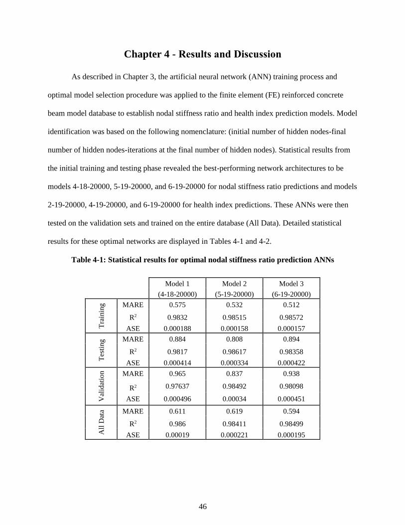
46

Chapter 4 - Results and Discussion

As described in Chapter 3, the artificial neural network (ANN) training process and

optimal model selection procedure was applied to the finite element (FE) reinforced concrete

beam model database to establish nodal stiffness ratio and health index prediction models. Model

identification was based on the following nomenclature: (initial number of hidden nodes-final

number of hidden nodes-iterations at the final number of hidden nodes). Statistical results from

the initial training and testing phase revealed the best-performing network architectures to be

models 4-18-20000, 5-19-20000, and 6-19-20000 for nodal stiffness ratio predictions and models

2-19-20000, 4-19-20000, and 6-19-20000 for health index predictions. These ANNs were then

tested on the validation sets and trained on the entire database (All Data). Detailed statistical

results for these optimal networks are displayed in Tables 4-1 and 4-2.

Table 4-1: Statistical results for optimal nodal stiffness ratio prediction ANNs

Model 1 Model 2 Model 3

(4-18-20000) (5-19-20000) (6-19-20000)

Tra

inin

g

MARE 0.575 0.532 0.512

R2 0.9832 0.98515 0.98572

ASE 0.000188 0.000158 0.000157

Tes

ting MARE 0.884 0.808 0.894

R2 0.9817 0.98617 0.98358

ASE 0.000414 0.000334 0.000422

Val

idat

ion

MARE 0.965 0.837 0.938

R2 0.97637 0.98492 0.98098

ASE 0.000496 0.00034 0.000451

All

Dat

a MARE 0.611 0.619 0.594

R2 0.986 0.98411 0.98499

ASE 0.00019 0.000221 0.000195

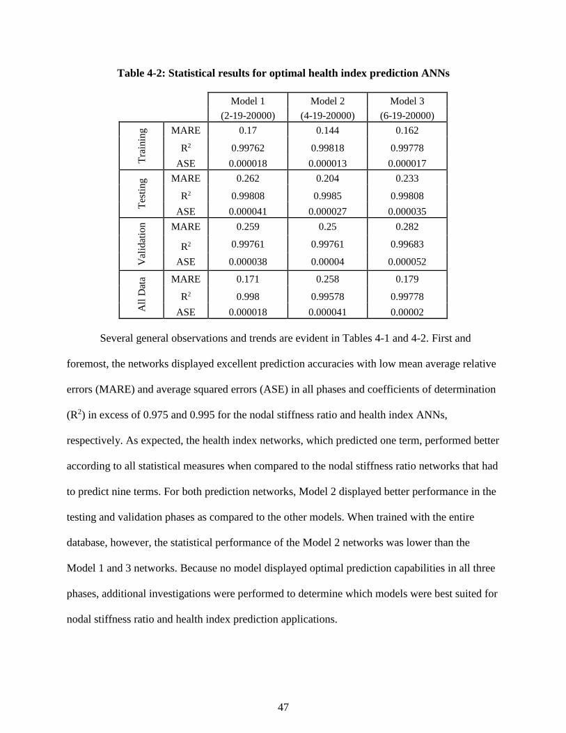
47

Table 4-2: Statistical results for optimal health index prediction ANNs

Model 1 Model 2 Model 3

(2-19-20000) (4-19-20000) (6-19-20000)

Tra

inin

g

MARE 0.17 0.144 0.162

R2 0.99762 0.99818 0.99778

ASE 0.000018 0.000013 0.000017

Tes

tin

g MARE 0.262 0.204 0.233

R2 0.99808 0.9985 0.99808

ASE 0.000041 0.000027 0.000035

Val

idat

ion

MARE 0.259 0.25 0.282

R2 0.99761 0.99761 0.99683

ASE 0.000038 0.00004 0.000052

All

Dat

a MARE 0.171 0.258 0.179

R2 0.998 0.99578 0.99778

ASE 0.000018 0.000041 0.00002

Several general observations and trends are evident in Tables 4-1 and 4-2. First and

foremost, the networks displayed excellent prediction accuracies with low mean average relative

errors (MARE) and average squared errors (ASE) in all phases and coefficients of determination

(R2) in excess of 0.975 and 0.995 for the nodal stiffness ratio and health index ANNs,

respectively. As expected, the health index networks, which predicted one term, performed better

according to all statistical measures when compared to the nodal stiffness ratio networks that had

to predict nine terms. For both prediction networks, Model 2 displayed better performance in the

testing and validation phases as compared to the other models. When trained with the entire

database, however, the statistical performance of the Model 2 networks was lower than the

Model 1 and 3 networks. Because no model displayed optimal prediction capabilities in all three

phases, additional investigations were performed to determine which models were best suited for

nodal stiffness ratio and health index prediction applications.

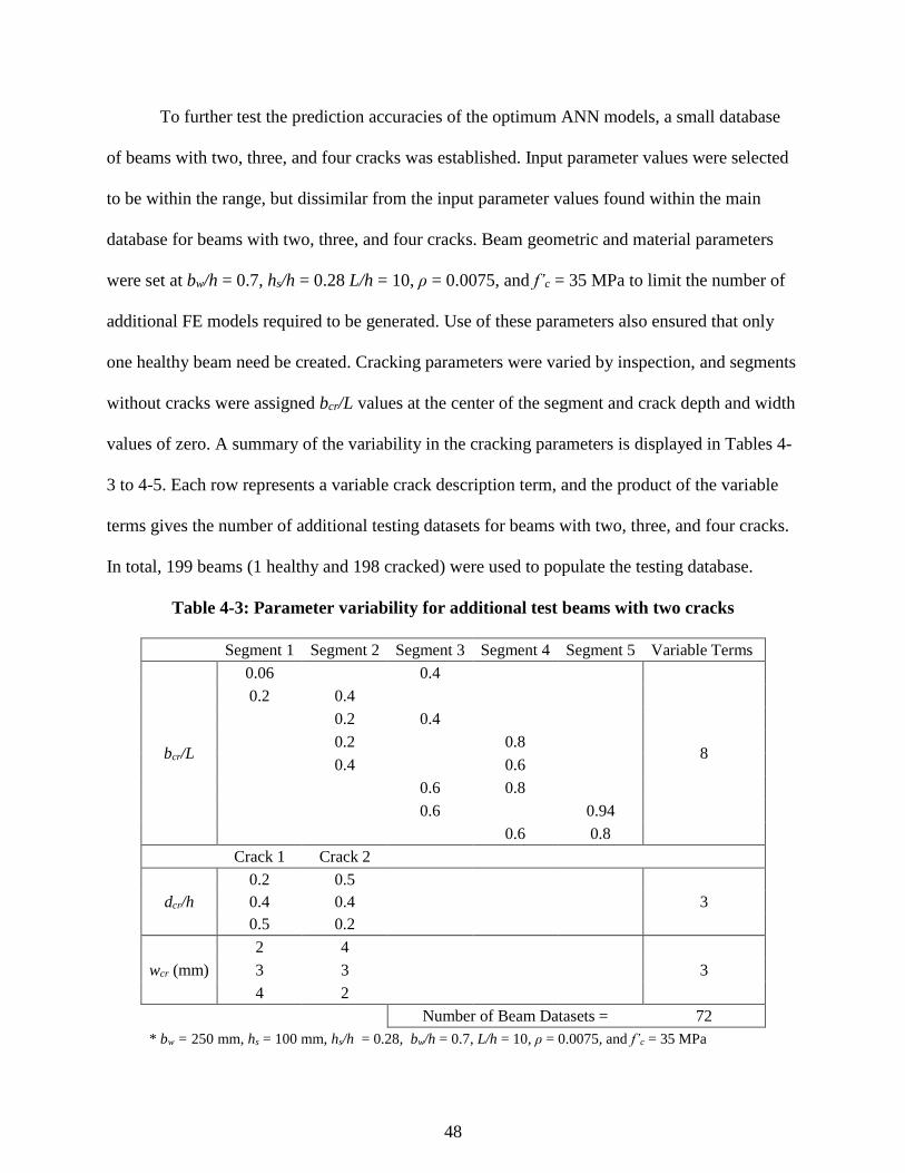
48

To further test the prediction accuracies of the optimum ANN models, a small database

of beams with two, three, and four cracks was established. Input parameter values were selected

to be within the range, but dissimilar from the input parameter values found within the main

database for beams with two, three, and four cracks. Beam geometric and material parameters

were set at bw/h = 0.7, hs/h = 0.28 L/h = 10, ρ = 0.0075, and f’c = 35 MPa to limit the number of

additional FE models required to be generated. Use of these parameters also ensured that only

one healthy beam need be created. Cracking parameters were varied by inspection, and segments

without cracks were assigned bcr/L values at the center of the segment and crack depth and width

values of zero. A summary of the variability in the cracking parameters is displayed in Tables 4-

3 to 4-5. Each row represents a variable crack description term, and the product of the variable

terms gives the number of additional testing datasets for beams with two, three, and four cracks.

In total, 199 beams (1 healthy and 198 cracked) were used to populate the testing database.

Table 4-3: Parameter variability for additional test beams with two cracks

Segment 1 Segment 2 Segment 3 Segment 4 Segment 5 Variable Terms

bcr/L

0.06 0.4

8

0.2 0.4

0.2 0.4

0.2 0.8

0.4 0.6

0.6 0.8

0.6 0.94

0.6 0.8

Crack 1 Crack 2

dcr/h

0.2 0.5

3 0.4 0.4

0.5 0.2

wcr (mm)

2 4

3 3 3

4 2

Number of Beam Datasets = 72

* bw = 250 mm, hs = 100 mm, hs/h = 0.28, bw/h = 0.7, L/h = 10, ρ = 0.0075, and f’c = 35 MPa

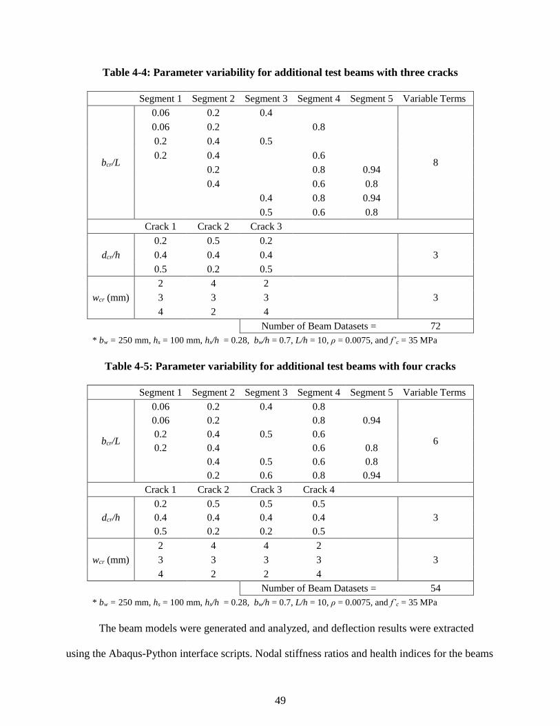
49

Table 4-4: Parameter variability for additional test beams with three cracks

Segment 1 Segment 2 Segment 3 Segment 4 Segment 5 Variable Terms

bcr/L

0.06 0.2 0.4

8

0.06 0.2 0.8

0.2 0.4 0.5

0.2 0.4 0.6

0.2 0.8 0.94

0.4 0.6 0.8

0.4 0.8 0.94

0.5 0.6 0.8

Crack 1 Crack 2 Crack 3

dcr/h

0.2 0.5 0.2

3 0.4 0.4 0.4

0.5 0.2 0.5

wcr (mm)

2 4 2

3 3 3 3

4 2 4

Number of Beam Datasets = 72

* bw = 250 mm, hs = 100 mm, hs/h = 0.28, bw/h = 0.7, L/h = 10, ρ = 0.0075, and f’c = 35 MPa

Table 4-5: Parameter variability for additional test beams with four cracks

Segment 1 Segment 2 Segment 3 Segment 4 Segment 5 Variable Terms

bcr/L

0.06 0.2 0.4 0.8

6

0.06 0.2 0.8 0.94

0.2 0.4 0.5 0.6

0.2 0.4 0.6 0.8

0.4 0.5 0.6 0.8

0.2 0.6 0.8 0.94

Crack 1 Crack 2 Crack 3 Crack 4

dcr/h

0.2 0.5 0.5 0.5

3 0.4 0.4 0.4 0.4

0.5 0.2 0.2 0.5

wcr (mm)

2 4 4 2

3 3 3 3 3

4 2 2 4

Number of Beam Datasets = 54

* bw = 250 mm, hs = 100 mm, hs/h = 0.28, bw/h = 0.7, L/h = 10, ρ = 0.0075, and f’c = 35 MPa

The beam models were generated and analyzed, and deflection results were extracted

using the Abaqus-Python interface scripts. Nodal stiffness ratios and health indices for the beams

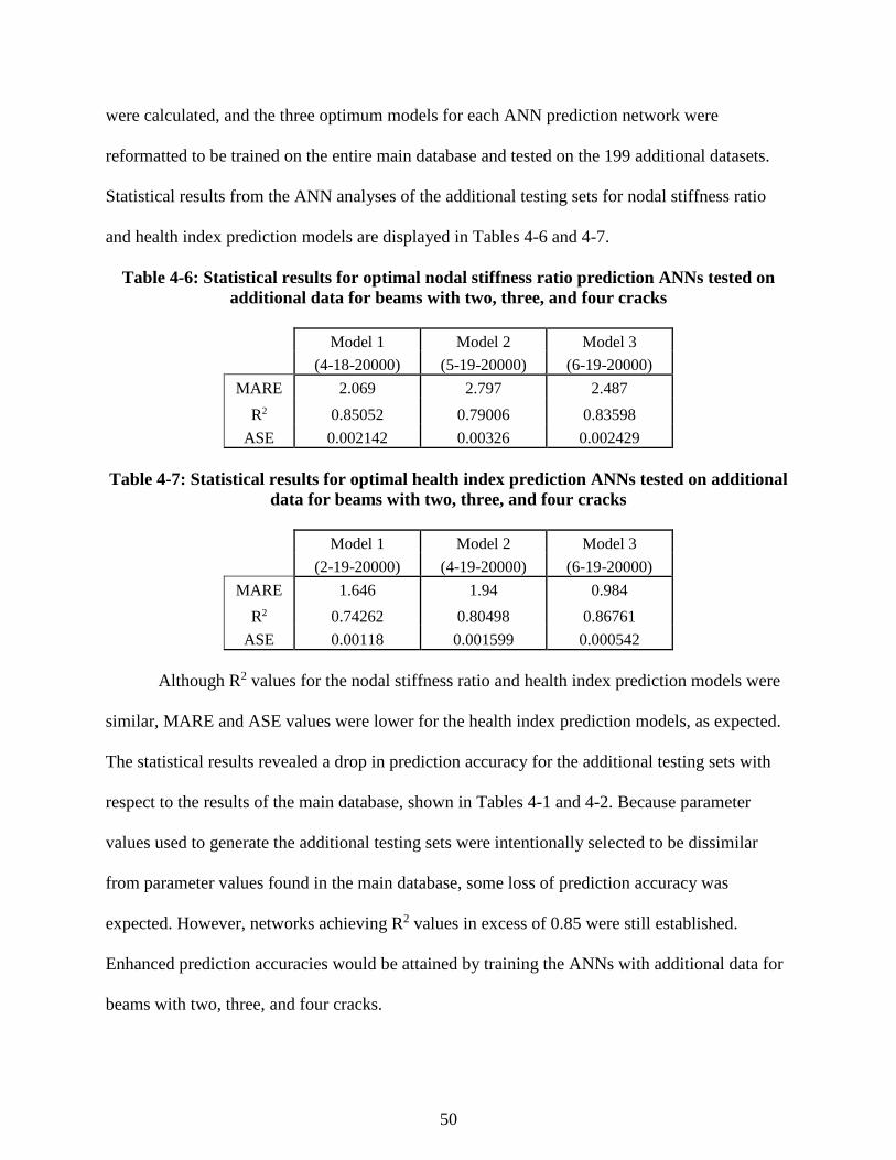
50

were calculated, and the three optimum models for each ANN prediction network were

reformatted to be trained on the entire main database and tested on the 199 additional datasets.

Statistical results from the ANN analyses of the additional testing sets for nodal stiffness ratio

and health index prediction models are displayed in Tables 4-6 and 4-7.

Table 4-6: Statistical results for optimal nodal stiffness ratio prediction ANNs tested on

additional data for beams with two, three, and four cracks

Model 1 Model 2 Model 3

(4-18-20000) (5-19-20000) (6-19-20000)

MARE 2.069 2.797 2.487

R2 0.85052 0.79006 0.83598

ASE 0.002142 0.00326 0.002429

Table 4-7: Statistical results for optimal health index prediction ANNs tested on additional

data for beams with two, three, and four cracks

Model 1 Model 2 Model 3

(2-19-20000) (4-19-20000) (6-19-20000)

MARE 1.646 1.94 0.984

R2 0.74262 0.80498 0.86761

ASE 0.00118 0.001599 0.000542

Although R2 values for the nodal stiffness ratio and health index prediction models were

similar, MARE and ASE values were lower for the health index prediction models, as expected.

The statistical results revealed a drop in prediction accuracy for the additional testing sets with

respect to the results of the main database, shown in Tables 4-1 and 4-2. Because parameter

values used to generate the additional testing sets were intentionally selected to be dissimilar

from parameter values found in the main database, some loss of prediction accuracy was

expected. However, networks achieving R2 values in excess of 0.85 were still established.

Enhanced prediction accuracies would be attained by training the ANNs with additional data for

beams with two, three, and four cracks.

51

Dr. Najjar recommended that the additional testing sets of beams with two, three, and

four cracks be exchanged with random beams from the training sets of the main database in order

to verify the ANNs (Y. Najjar, personal communication, December 11, 2015). The ANN training

process and optimal model selection procedure was applied to the adjusted data to establish

health index prediction networks, and the three optimum models were trained on the altered

database and tested on the 199 exchanged beams. The statistical results were excellent with low

errors and R2 values exceeding 0.99 for all health index prediction models. Testing results for the

exchanged beams are displayed in Table 4-8.

Table 4-8: Statistical results for optimal health index ANNs trained on altered database

and tested on exchanged beam sets

Model 1 Model 2 Model 3

(4-19-5400) (6-17-9100) (10-19-6000)

MARE 0.297 0.245 0.227

R2 0.99823 0.99818 0.99869

ASE 0.000052 0.000032 0.000028

As previously described, the datasets for beams with two, three, and four cracks were

successfully used to test the optimum ANN models’ prediction accuracies on dissimilar data.

However, it was desired that the networks be tested on entirely random data in order to obtain an

unbiased assessment of the models’ prediction capabilities. Therefore, 75 cracked beam datasets,

corresponding to equal numbers of beams with 1–5 cracks, were generated using Microsoft

Excel’s RAND() function to establish the value of each input parameter. Seventy-five healthy

beam datasets with geometric and material parameters identical to those of the cracked beams

were also generated to serve as references for the calculation of nodal stiffness ratios and health

indices. Input and output parameter values for these random testing sets are included in

Appendix D. FE models were created and analyzed, deflection results were extracted, and nodal

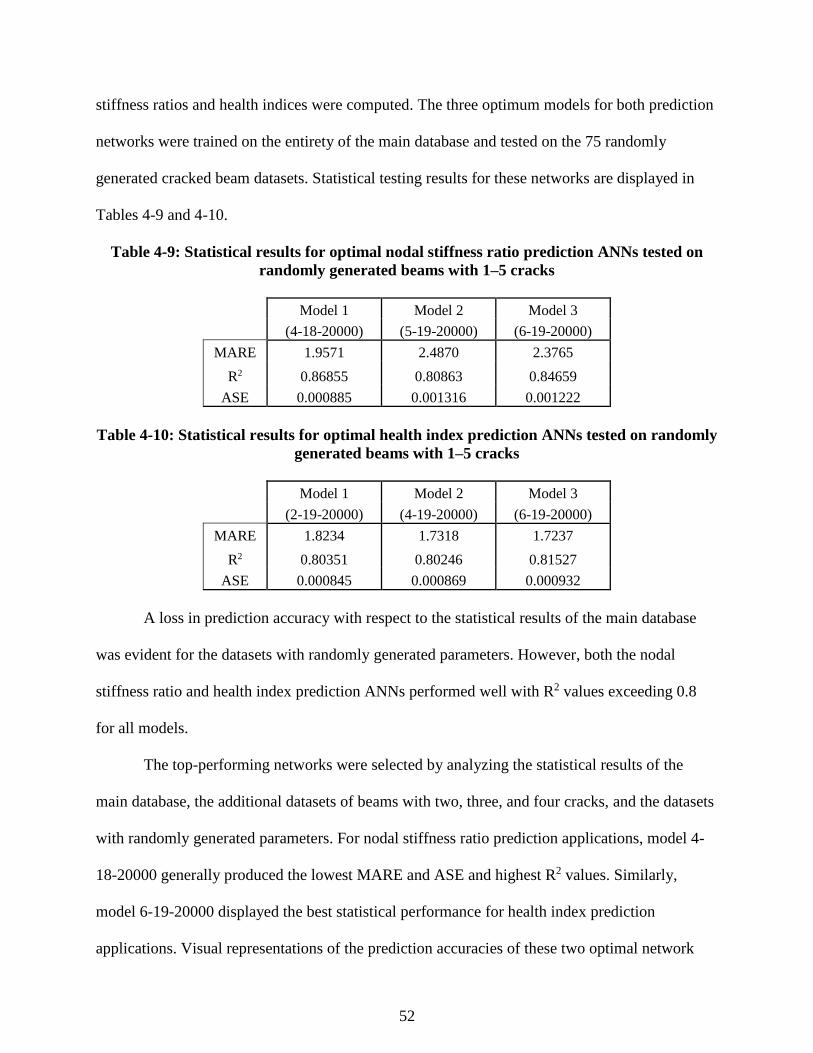
52

stiffness ratios and health indices were computed. The three optimum models for both prediction

networks were trained on the entirety of the main database and tested on the 75 randomly

generated cracked beam datasets. Statistical testing results for these networks are displayed in

Tables 4-9 and 4-10.

Table 4-9: Statistical results for optimal nodal stiffness ratio prediction ANNs tested on

randomly generated beams with 1–5 cracks

Model 1 Model 2 Model 3

(4-18-20000) (5-19-20000) (6-19-20000)

MARE 1.9571 2.4870 2.3765

R2 0.86855 0.80863 0.84659

ASE 0.000885 0.001316 0.001222

Table 4-10: Statistical results for optimal health index prediction ANNs tested on randomly

generated beams with 1–5 cracks

Model 1 Model 2 Model 3

(2-19-20000) (4-19-20000) (6-19-20000)

MARE 1.8234 1.7318 1.7237

R2 0.80351 0.80246 0.81527

ASE 0.000845 0.000869 0.000932

A loss in prediction accuracy with respect to the statistical results of the main database

was evident for the datasets with randomly generated parameters. However, both the nodal

stiffness ratio and health index prediction ANNs performed well with R2 values exceeding 0.8

for all models.

The top-performing networks were selected by analyzing the statistical results of the

main database, the additional datasets of beams with two, three, and four cracks, and the datasets

with randomly generated parameters. For nodal stiffness ratio prediction applications, model 4-

18-20000 generally produced the lowest MARE and ASE and highest R2 values. Similarly,

model 6-19-20000 displayed the best statistical performance for health index prediction

applications. Visual representations of the prediction accuracies of these two optimal network

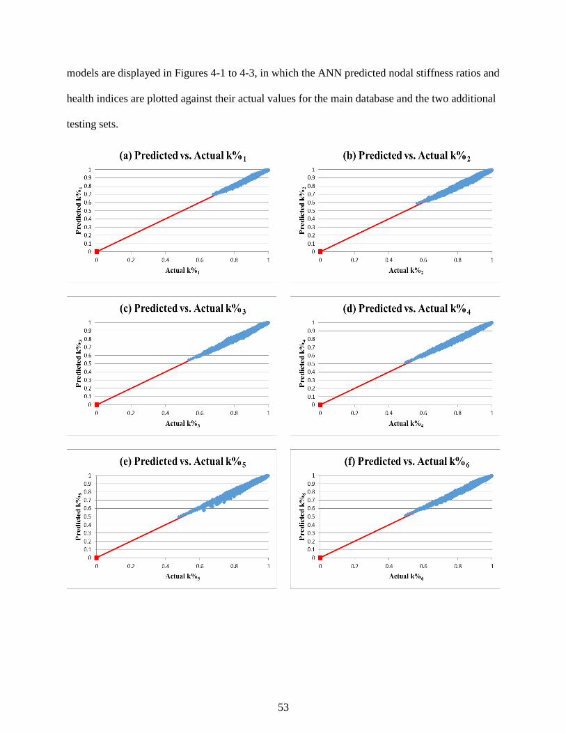
53

models are displayed in Figures 4-1 to 4-3, in which the ANN predicted nodal stiffness ratios and

health indices are plotted against their actual values for the main database and the two additional

testing sets.

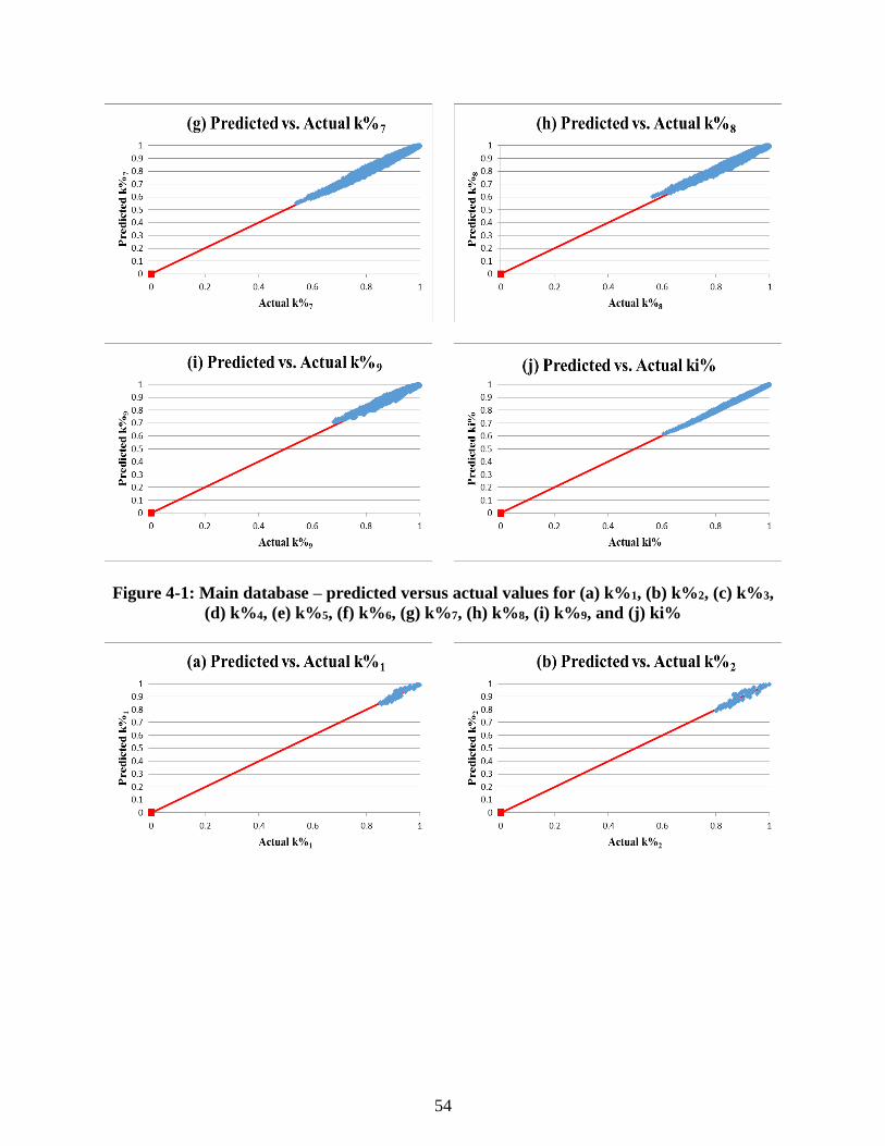
54

Figure 4-1: Main database – predicted versus actual values for (a) k%1, (b) k%2, (c) k%3,

(d) k%4, (e) k%5, (f) k%6, (g) k%7, (h) k%8, (i) k%9, and (j) ki%

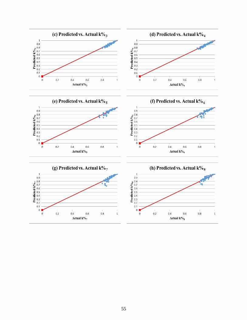
55

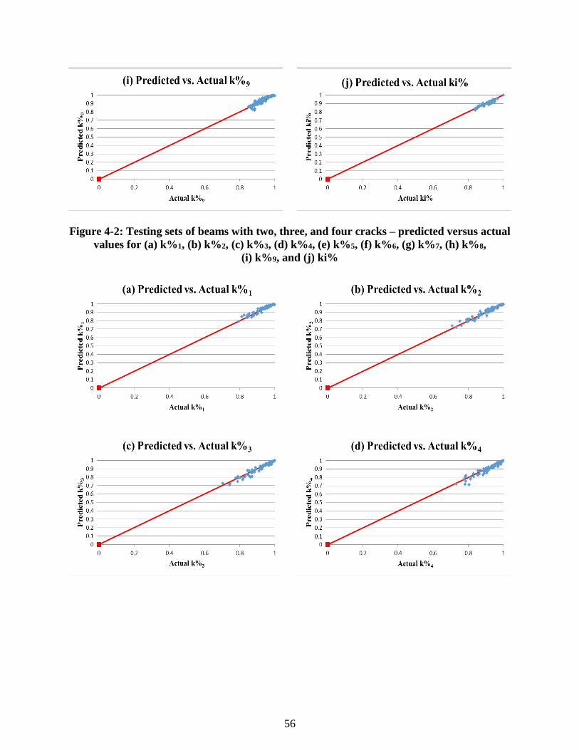
56

Figure 4-2: Testing sets of beams with two, three, and four cracks – predicted versus actual

values for (a) k%1, (b) k%2, (c) k%3, (d) k%4, (e) k%5, (f) k%6, (g) k%7, (h) k%8,

(i) k%9, and (j) ki%

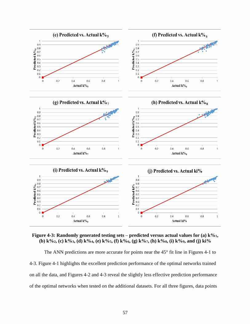
57

Figure 4-3: Randomly generated testing sets – predicted versus actual values for (a) k%1,

(b) k%2, (c) k%3, (d) k%4, (e) k%5, (f) k%6, (g) k%7, (h) k%8, (i) k%9, and (j) ki%

The ANN predictions are more accurate for points near the 45° fit line in Figures 4-1 to

4-3. Figure 4-1 highlights the excellent prediction performance of the optimal networks trained

on all the data, and Figures 4-2 and 4-3 reveal the slightly less effective prediction performance

of the optimal networks when tested on the additional datasets. For all three figures, data points

58

for the health index prediction model were very close to the 45° fit line, suggesting that ANNs

provide excellent prediction capabilities when predicting a single measure of damage for the

beams. The figures also show that accuracy of the nodal stiffness ratio prediction model

decreased for nodes close to the center of the beam. Because these nodes typically have low

nodal stiffness ratios, this loss of accuracy may correlate to reduced ANN prediction accuracies

for heavily damaged sections. Although these results indicate that special considerations need be

taken when using the optimum ANN models to evaluate the structural health of significantly

damaged beams, the networks generally provide conservative predictions, somewhat reducing

the impact of potential inaccuracies. This is evident in Figures 4-2 and 4-3 where the lower

magnitude nodal stiffness ratios often fall below the 45° line, indicating that the predicted

stiffness ratios are lower than the actual values. The generally tight spread of the data points

about the 45° lines in Figures 4-1 to 4-3 affirms the effectiveness of the optimal ANN models for

nodal stiffness ratio and health index prediction applications.

59

Chapter 5 - ANN User Interface Application

After applying the artificial neural network (ANN) training process and optimum model

selection procedure and evaluating the top-performing models’ prediction accuracies on

additional testing datasets, the optimal ANN architectures for nodal stiffness ratio and health

index prediction applications were established. Biases and connection weights for the input

layer-hidden layer and hidden layer-output layer were retrieved after these network structures

were trained on all the data in the main database. Application of these biases and connection

weights to the summation and activation functions described in Equations 2-1 and 2-2 allowed

for calculation of the ANN-predicted nodal stiffness ratios and health index for any simply-

supported reinforced concrete T-beam having parameters within the range of those used to create

the finite element (FE) model database. In order to automate these calculations and facilitate on-

site damage evaluation using the optimal ANN models, a touch user-interface driven electronic

application was developed.

Several development platform options were considered for the ANN touch user-interface,

including a computer application written in Python, a Visual Studio Windows Presentation

Foundation (WPF) computer application, a web-based application written in JavaScript, and

Android and/or Apple mobile application(s). Many Python graphical user interface application

frameworks are cross-platform, but the interface construction tools are limited for some

frameworks. Although WPF applications are limited to Microsoft Windows computers, Visual

Studio offers vast library of interface construction tools. Web-based JavaScript applications are

touted as relatively easy to develop, but the fact they generally require internet connectivity to

function restricts their field use. Although mobile platforms provide clean and simple user

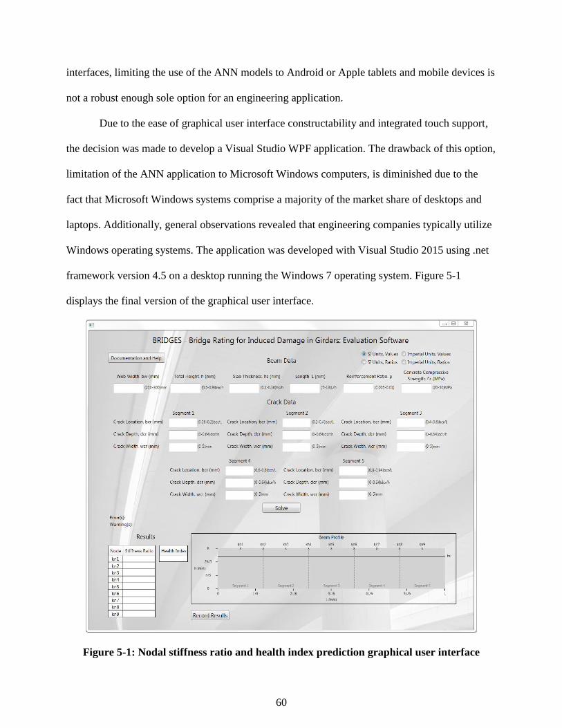
60

interfaces, limiting the use of the ANN models to Android or Apple tablets and mobile devices is

not a robust enough sole option for an engineering application.

Due to the ease of graphical user interface constructability and integrated touch support,

the decision was made to develop a Visual Studio WPF application. The drawback of this option,

limitation of the ANN application to Microsoft Windows computers, is diminished due to the

fact that Microsoft Windows systems comprise a majority of the market share of desktops and

laptops. Additionally, general observations revealed that engineering companies typically utilize

Windows operating systems. The application was developed with Visual Studio 2015 using .net

framework version 4.5 on a desktop running the Windows 7 operating system. Figure 5-1

displays the final version of the graphical user interface.

Figure 5-1: Nodal stiffness ratio and health index prediction graphical user interface

61

As shown in Figure 5-1, the user interface accepts geometric and material parameters (bw,

h, hs, L, ρ, and f’c) in the “Beam Data” section and cracking parameters (bcrn, dcrn, and wcrn) in the

“Crack Data” section as inputs. Upon activation of the “Solve” button, the input parameters are

normalized to function as input nodes for the ANN calculations. The biases and connection

weights from the optimum nodal stiffness ratio and health index ANN models are applied to pass

the input parameters to the hidden nodes and ultimately to the output nodes. The output

parameters are then de-normalized, and the predicted nodal stiffness ratios and health index are

displayed in the tables in the “Results” section at the lower left corner of the user interface. Also

after pressing the “Solve” button, the “Beam Profile” is updated to display the location of the

flange of the T-beam and the location and depth of each crack. The height and length labels are

also changed to reflect the user-input height and length of the beam. Because the stiffness nodes

are equidistant fractions of the span length of the beam, the “x” and “kn” labels for the stiffness

nodes are static and serve as a visual reference for the location of the tabulated stiffness ratios.

Similarly, the “Segment” labels and dashed lines are static and graphically display the five equal

segments into which the beam is divided. Selection of the “SI Units” and “Imperial Units” radio

buttons in the upper right corner of the interface change the parameter unit and range labels and

automatically alter the ANN calculations for the selected measurement system. The “SI Units,

Ratios” and “Imperial Units, Ratios” radio buttons allow the program to accept crack locations

and depths as ratios of the length and height of the beam, respectively, instead of absolute values.

Once calculations have been run and results are displayed in the tables, selection of the

“Record Results” button writes the beam’s input properties and health results to a text file and

opens the file with the computer’s default text editor. The space to the right of the “Record

Results” button displays the name of the results file and the directory in which the file is stored;

62

the directory from which the application’s executable file is being run. Similarly, selection of the

“Documentation and Help” button opens a read-only text file and stores the file in the

application’s working directory. This text file contains information about the development of the

damage evaluation application and instructions on how to use the program, including a

description of the range of parameter values on which the ANN models were trained. If the user

enters data outside the applicable parameter value training ranges, selection of the “Solve” button

causes text to fill the “Warning(s):” label indicating which parameters produced warnings.

Although the program will run if warnings are present, use of parameter values outside the range

of the training data may produce unreliable results. In addition to being described in the

“Documentation and Help” file, the parameter value ranges are displayed next to the input text

box for each parameter. If errors are present, the program will not run and new results will not be

recorded. Errors can occur by failing to enter values in all text boxes of the “Beam Data” section.

Setting crack locations to values outside their applicable segment will also produce an error. In

an effort to minimize errors, if the user fails to enter data, or enters zero for any of the crack

locations, depths, or widths in the “Crack Data” section, the crack location value defaults to the

center of the segment and the depth and width values for the crack in that segment are set to zero.

This application was created to serve as an in-situ bridge member damage evaluation

tool. Because the application was developed using the Visual Studio WPF framework, the

program is intended to be compatible with Windows 7 or newer touch-enabled devices and

works with both touch or conventional mouse and keyboard input. To illustrate the functionality

of the program, the following figures display the interface window after solving for the nodal

stiffness ratios and health indices of two damaged reinforced concrete T-beams. The beam

solutions in Figures 5-2 and 5-3 correspond to cracked beams from the main training database

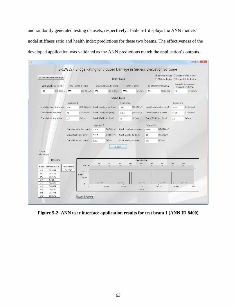
63

and randomly generated testing datasets, respectively. Table 5-1 displays the ANN models’

nodal stiffness ratio and health index predictions for these two beams. The effectiveness of the

developed application was validated as the ANN predictions match the application’s outputs.

Figure 5-2: ANN user interface application results for test beam 1 (ANN ID 8400)

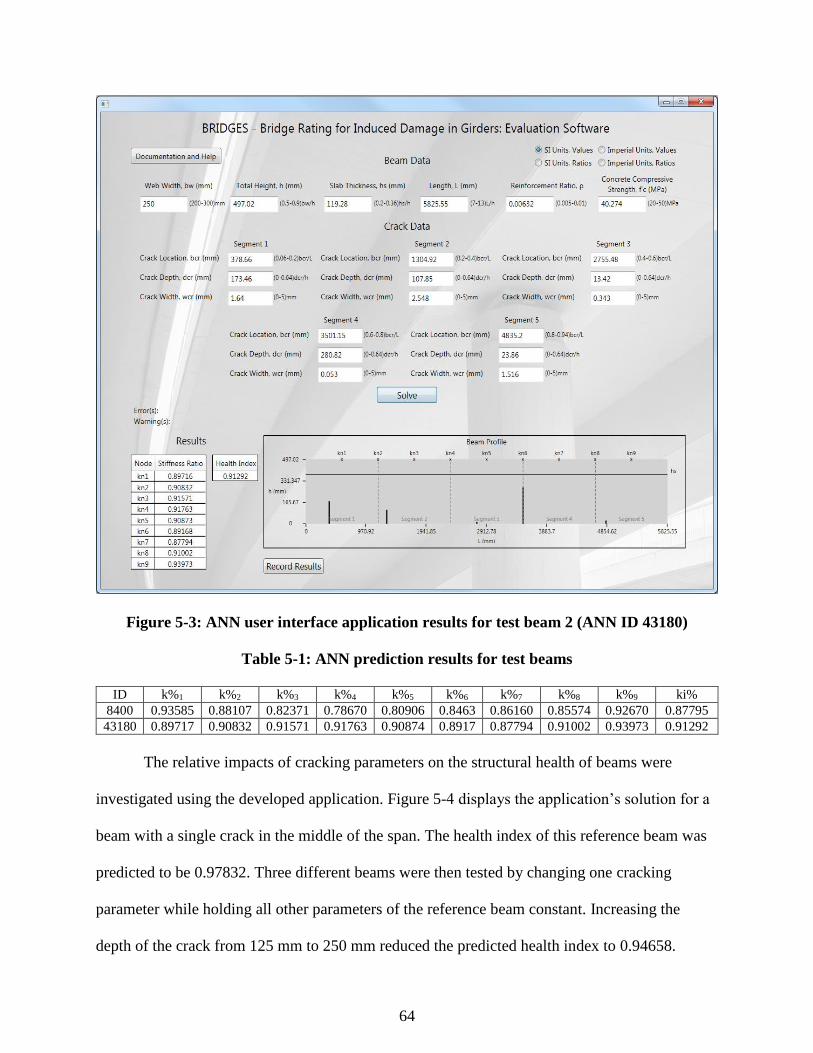
64

Figure 5-3: ANN user interface application results for test beam 2 (ANN ID 43180)

Table 5-1: ANN prediction results for test beams

ID k%1 k%2 k%3 k%4 k%5 k%6 k%7 k%8 k%9 ki%

8400 0.93585 0.88107 0.82371 0.78670 0.80906 0.8463 0.86160 0.85574 0.92670 0.87795

43180 0.89717 0.90832 0.91571 0.91763 0.90874 0.8917 0.87794 0.91002 0.93973 0.91292

The relative impacts of cracking parameters on the structural health of beams were

investigated using the developed application. Figure 5-4 displays the application’s solution for a

beam with a single crack in the middle of the span. The health index of this reference beam was

predicted to be 0.97832. Three different beams were then tested by changing one cracking

parameter while holding all other parameters of the reference beam constant. Increasing the

depth of the crack from 125 mm to 250 mm reduced the predicted health index to 0.94658.

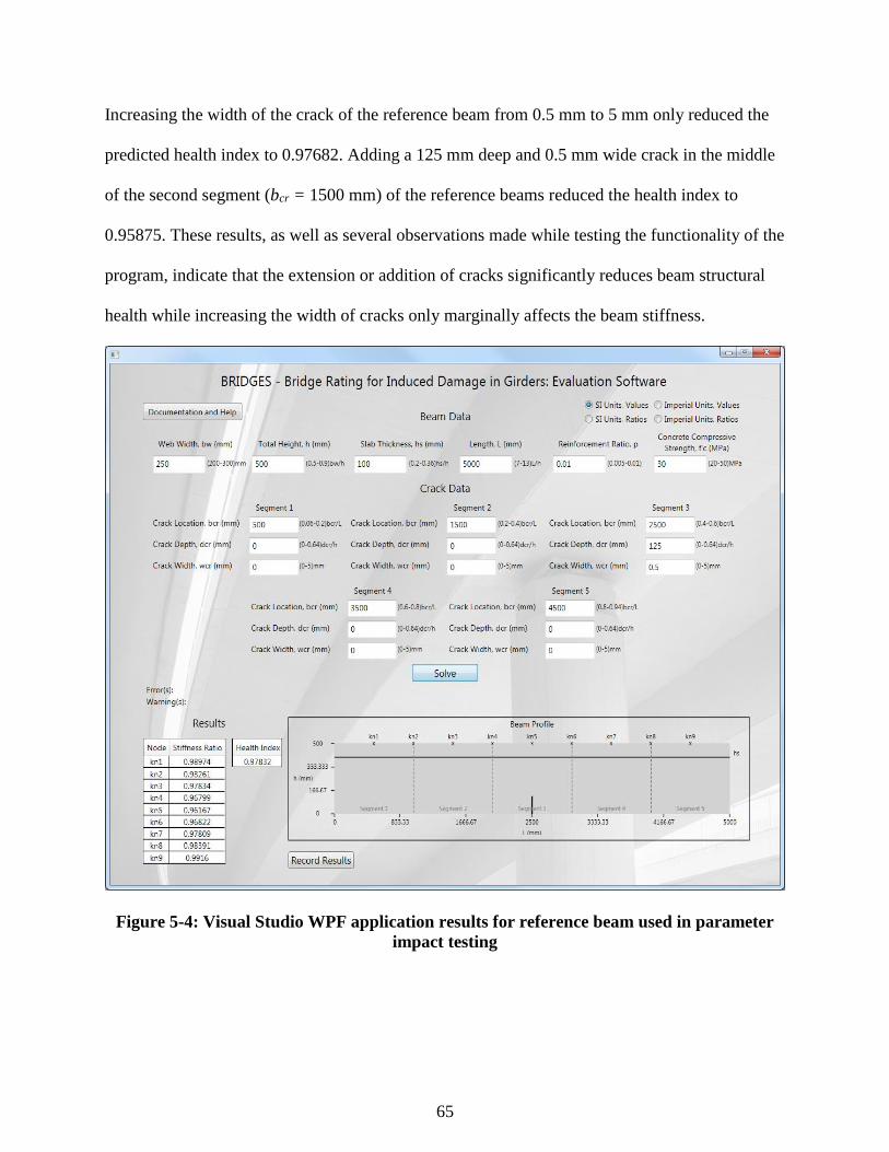
65

Increasing the width of the crack of the reference beam from 0.5 mm to 5 mm only reduced the

predicted health index to 0.97682. Adding a 125 mm deep and 0.5 mm wide crack in the middle

of the second segment (bcr = 1500 mm) of the reference beams reduced the health index to

0.95875. These results, as well as several observations made while testing the functionality of the

program, indicate that the extension or addition of cracks significantly reduces beam structural

health while increasing the width of cracks only marginally affects the beam stiffness.

Figure 5-4: Visual Studio WPF application results for reference beam used in parameter

impact testing

66

Chapter 6 - Conclusions and Recommendations

Conclusions

This research project investigated the potential for application of the finite element (FE)

method and artificial neural networks (ANNs) to create an objective damage evaluation model

for reinforced concrete T-girders that could be utilized with visual inspection crack inputs. A

review of the literature identified the need for accurate damage evaluation of deteriorating

infrastructure, discussed the drawbacks in the commonly applied visual inspection and condition

rating method, and reviewed various structural health monitoring (SHM) techniques for damage

evaluation and structural health prediction. A three-dimensional (3D) reinforced concrete T-

beam FE model database was constructed using Abaqus FE analysis software. Geometric (bw/h,

hs/h, L/h, and ρ), material (f’c), and cracking (bcr,m/L, dcr,m/h, and wcr,m) parameters varied

between the models, and up to five cracks were allowed per beam. Damage evaluation measures

were then computed, including the stiffness ratios of cracked to healthy beams with identical

geometric and material properties at nine equidistant nodes along the beams (k%n) and the health

index parameter (ki%), which is an integration of the nodal stiffness ratio profile across the beam

span length. Since most parameters were normalized with respect to a beam web width of 250

mm, a random sample of the database, holding constant the normalized geometric, material, and

cracking parameters, was generated for beams with web widths of 200 mm and 300 mm. Health

indices for these beams displayed good agreement with the results for the reference beams.

Coefficients of determination (R2) and Lin’s concordance correlation coefficients exceeding 0.99

and 0.975, respectively, indicated that the results of this study are reproducible for a variety of

beam sizes.

67

A feedforward ANN program utilizing a backpropagation learning algorithm was

employed to establish structural health prediction models based on the data in the reinforced

concrete T-beam database. The ANNs accepted the geometric, material, and cracking parameters

as inputs and predicted the nodal stiffness ratios or health indices as outputs. A distinct ANN

training process and optimal model selection procedure was followed to determine the optimum

models for nodal stiffness ratio and health index prediction applications. Statistical results for

these optimum models were excellent with R2 values exceeding 0.99 in the training, testing, and

validation phases. Additional FE model datasets with dissimilar and randomly generated input

parameters were constructed, and the prediction capabilities of the fully-trained optimum models

were assessed on the new datasets. The top-performing nodal stiffness ratio and health index

prediction models displayed good statistical performance with R2 values of 0.851 and 0.868 for

the dissimilar parameter datasets, and R2 values of 0.869 and 0.815 for the randomly generated

parameter datasets, respectively. Utilizing these two top-performing network architectures, a

touch-enabled application was developed to serve as an on-site damage evaluation tool. This

application has been given the acronym BRIDGES, which stands for Bridge Rating for Induced

Damage in Girders: Evaluation Software. This research demonstrated the effective application of

FE modeling and ANNs in SHM for objective damage evaluation. Statistical results of this study

indicate that ANN models can provide accurate predictions for the structural health of damaged

reinforced concrete T-beams. The theory and techniques utilized in this study can be applied to

any number of structural elements and SHM processes.

68

Recommendations

The following recommendations address the potential for refinement or expansion of this

research:

Further investigate the effects of different beam web widths: Analysis of the sample of

beams with different web widths revealed that the results of this study are reasonably

applicable to a variety of typical girder sizes. Further analysis could expand the

applicable size range or develop correction factors to adjust the results for beams with

different web widths.

Increase the size of the beam database: Because ANNs are data-driven tools, increasing

the amount of training data would enhance the model’s prediction accuracies. As stated in

Chapter 3, a large number of datasets were generated for beams with one crack.

Additional datasets could be generated for beams with two, three, four, and five cracks

with added crack configurations and more input parameter variation.

Expand the number of cracks per beam: This study considered beams with up to five

cracks. Although consideration of additional cracks would increase the complexity of the

problem and potentially decrease prediction accuracies of the networks unless the size of

the training database is increased exponentially, it would provide a more robust damage

evaluation tool for more severely damaged girders.

Add crack angle (θn) parameters: Only flexural cracks were analyzed as a result of this

research. Addition of angled cracks to the database would allow for more accurate

damage evaluations of beams with shear or flexural-shear cracks.

Consider additional beam configurations: The beams in this research were limited to

simply-supported concrete T-beams reinforced with steel rebar. The processes described

69

in the methodology could be applied to beams with different support types, such as multi-

span continuous beams, and various reinforcement types, such as pretressing strands or

fiber reinforced polymers. Other structural units, such as slabs, could also be investigated.

Compare with experimental data: Comparing the ANN models’ structural health

predictions with experimental test data could further validate the effectiveness of this

research technique. Such comparisons would also provide the opportunity to establish

damage metrics for the health index term. With further research, the health index could

be utilized as a standalone measure of structural health and dictate whether members are

structurally sound, should be more closely monitored, or require immediate repair or

replacement.

70

References

Ahlborn, T. M., Shuchman, R., Sutter, L. L., Brooks, C. N., Harris, D. H., Burns, J. W., Endsley,

K. A., Evans, D. C., Vaghefi, K., & Oats, R. C. (2010). The state-of-the-practice of modern

structural health monitoring for bridges: A comprehensive review. Retrieved from the TRID

database.

Al-Ghalib, A., Mohammad, F., Rahman, M., & Chilton, J. (2011, September 26–28). Damage

and repair quantification in reinforced concrete beams using vibration data. Paper

presented at the 4th International Conference on Concrete Repair: Concrete Solutions.

Dresden, Germany. Retrieved from Compendex database. (T20:47:24Z).

Al-Rahmani, A. (2012). A combined soft computing-mechanics approach to damage evaluation

and detection in reinforced concrete beams (Master’s thesis). Kansas State University,

Manhattan, Kansas.

Al-Rahmani, A., Rasheed, H., & Najjar, Y. (2013). Intelligent damage detection in bridge

girders: Hybrid approach. Journal of Engineering Mechanics, 139(3), 296-304. doi:

10.1061/(ASCE)EM.1943-7889.0000536

Al-Rahmani, A., Rasheed, H., & Najjar, Y. (2014). An artificial intelligence approach to

objective health monitoring and damage detection in concrete bridge girders. American

Concrete Institute Special Publication, 298(6), 73-89.

American Concrete Institute Committee 318. (2014). Building code requirements for structural

concrete and commentary. (ACI No. 318R-14). Farmington Hills, MI: American Concrete

Institute.

71

American Society of Civil Engineers. (2013). 2013 report card for America's infrastructure.

Reston, VA, United States: American Society of Civil Engineers. Retrieved from

http://www.infrastructurereportcard.org/bridges/

Basheer, I., A. (1998). Neuromechanistic-based modeling and simulation of constitutive

behavior of fine-grained soils (Doctoral Dissertation). Kansas State University, Manhattan,

Kansas.

Beer, F. P., Johnston, E. R., Dewolf, J. T., & Mazurek, D. F. (2012). Mechanics of Materials (6th

ed.). New York, NY: McGraw-Hill Companies, Inc.

Chen, S., Liu, W., Bian, H., & Smith, B. (2012, October 31–November 3). 3D LiDAR scans for

bridge damage evaluation. Paper presented at the 6th Congress on Forensic Engineering:

Gateway to a Better Tomorrow. San Francisco, CA, United States.

doi:10.1061/9780784412640.052

Dassault Systèmes Simulia Corp. (2013). Abaqus 6.13 [computer software]. Providence, RI:

Dassault Systèmes.

Farhidzadeh, A., Dehghan-Niri, E., Moustafa, A., Salamone, S., & Whittaker, A. (2013).

Damage assessment of reinforced concrete structures using fractal analysis of residual crack

patterns. Experimental Mechanics, 53(9), 1607–1619. doi:10.1007/s11340-013-9769-7

Federal Highway Administration (a). (2014). Deficient bridges by state and highway system

[Microsoft Excel spreadsheet]. Retrieved from https://www.fhwa.dot.gov/bridge/britab.cfm

Federal Highway Administration (b). (2014). Structure type by state [Microsoft Excel

spreadsheet]. Retrieved from https://www.fhwa.dot.gov/bridge/britab.cfm

72

Gassman, S. L., & Tawhed, W. F. (2004). Nondestructive assessment of damage in concrete

bridge decks. Journal of Performance of Constructed Facilities, 18(4), 220–231.

doi:10.1061/(ASCE)0887-3828(2004)18:4(220)

Ghods, A. S., & Esfahani, M. R. (2009, July 22–24). Damage assessment of reinforced concrete

beams by modal test. Paper presented at the 4th International Conference on Structural

Health Monitoring of Intelligent Infrastructure. Zurich, Switzerland. Retrieved from

Compendex database.

Hasançebi, O., & Dumlupinar, T. (2013). Linear and nonlinear model updating of reinforced

concrete T-beam bridges using artificial neural networks. Computers & Structures, 119, 1–

11. doi:10.1016/j.compstruc.2012.12.017

Jeyasehar, C. A., & Sumangala, K. (2006). Damage assessment of prestressed concrete beams

using artificial neural network (ANN) approach. Computers & Structures, 84(26), 1709–

1718. doi:10.1016/j.compstruc.2006.03.005

Lenett, M. S., Griessmann, A., Helmicki, A. J., & Aktan, A. E. (1999). Subjective and objective

evaluations of bridge damage. Transportation Research Record, 1688, 76–86.

doi:10.3141/1688-10

Li, L., Ghrib, S., & Lee, S. (2008, Jun 10-13). Damage identification of reinforced concrete

beams by digital image correlation and FE-updating. Paper presented at the Canadian

Society for Civil Engineering Annual Conference: Partnership for Innovation. Quebec City,

QC, Canada. Retrieved from Compendex database.

Lin, L., I. (1989). A concordance correlation coefficient to evaluate reproducibility. Biometrics,

45. Retrieved from http://www.jstor.org/stable/2532051

73

Ndambi, J., Vantomme, J., & Harri, K. (2002). Damage assessment in reinforced concrete beams

using eigenfrequencies and mode shape derivatives. Engineering Structures, 24(4), 501–

515. doi:10.1016/S0141-0296(01)00117-1

Reynders, E., & De Roeck, G. (2009). A local flexibility method for vibration-based damage

localization and quantification. Journal of Sound and Vibration, 329(12), 2367–2383.

doi:10.1016/j.jsv.2009.04.026

Sagar, R. V., Prasad, B. K. R., & Sharma, R. (2012). Evaluation of damage in reinforced

concrete bridge beams using acoustic emission technique. Nondestructive Testing and

Evaluation, 27(2), 95–108. doi:10.1080/10589759.2011.610452

Shiotani, T., Ohtsu, H., Momoki, S., Chai, H. K., Onishi, H., & Kamada, T. (2012). Damage

evaluation for concrete bridge deck by means of stress wave techniques. Journal of Bridge

Engineering, 17(6), 847–856. doi:10.1061/(ASCE)BE.1943-5592.0000373

Sohn, H., Farrar, C. R., Hemez, F. M., Shunk, D. D., Stinemates, D. W., Nadler, B. R., &

Czarnecki, J. J. (2004). A review of structural health monitoring literature: 1996-2001. Los

Alamos National Laboratory report LA-13976-MS. Retrieved from

https://institute.lanl.gov/ei/publications/structural-health-monitoring/

Teughels, A., Maeck, J., & De Roeck, G. (2002). Damage assessment by FE model updating

using damage functions. Computers & Structures, 80(25), 1869–1879. doi:10.1016/S0045-

7949(02)00217-1

Yaserer, H., I. (2010). Characterizing the permeability of concrete mixes used in transportation

applications: A neuronet approach (Master’s thesis). Kansas State University, Manhattan,

Kansas.

74

Appendix A - Abaqus-Python Scripts

Example script for generation of a singly-cracked reinforced concrete T-beam:

from abaqus import *

from abaqusConstants import *

import __main__

import section

import regionToolset

import displayGroupMdbToolset as dgm

import part

import material

import assembly

import step

import interaction

import load

import mesh

import optimization

import job

import sketch

import visualization

import xyPlot

import displayGroupOdbToolset as dgo

import connectorBehavior

beamdb = open('beamdb1c.txt')

lines = beamdb.readlines()

dbp = []

for line in lines:

spline = line.split()

spline[0] = spline[0] + spline[1]

del spline[1]

dbp.append(spline)

knodes = 9

kns = [x/(knodes+1.0) for x in range(knodes+1.0)[1:]]

Lns = ['L'+str(x) for x in range (knodes+1)[1:]]

knsdict = dict(zip(kns,Lns))

for beam in dbp:

for kn in kns:

Mdb()

job = beam[0] + '-' + knsdict[kn]

bwbeam = 250.0

bwhratio = float(beam[1])

Lhratio = float(beam[3])

fconc = float(beam[5])

hbeam = bwbeam / bwhratio

Lbeam = hbeam * Lhratio

tfbeam = float(beam[2])*hbeam

hwbeam = hbeam - tfbeam

75

bfbeampos = hwbeam+bwbeam

bfbeamneg = -hwbeam

Econc = 4700.0 * fconc**0.5

vconc = 0.2

bcrLratio = float(beam[7])

dcrhratio = float(beam[8])

wcr = float(beam[9])

bcr = bcrLratio * Lbeam

dcr = dcrhratio * hbeam

xcr = -Lbeam/2+bcr-wcr/2

rho = float(beam[4])

cover = 50.0

d = hbeam - cover

As = rho*bwbeam*d

Ab = As/3

dbar = (Ab*4/pi)**0.5

'dbar = round(db)'

Abar = pi/4*dbar**2

Esteel = 200000.0

vsteel = 0.3

knode = kn

concmesh = 35.0

steelmesh = 35.0

load = 100000.0

s = mdb.models['Model-1'].ConstrainedSketch(name='__profile__',

sheetSize=200.0)

g, v, d, c = s.geometry, s.vertices, s.dimensions, s.constraints

s.setPrimaryObject(option=STANDALONE)

s.Line(point1=(0.0, 0.0), point2=(bwbeam, 0.0))

s.HorizontalConstraint(entity=g[2], addUndoState=False)

s.Line(point1=(bwbeam, 0.0), point2=(bwbeam, hwbeam))

s.VerticalConstraint(entity=g[3], addUndoState=False)

s.PerpendicularConstraint(entity1=g[2], entity2=g[3], addUndoState=False)

s.Line(point1=(bwbeam, hwbeam), point2=(bfbeampos, hwbeam))

s.HorizontalConstraint(entity=g[4], addUndoState=False)

s.PerpendicularConstraint(entity1=g[3], entity2=g[4], addUndoState=False)

s.Line(point1=(bfbeampos, hwbeam), point2=(bfbeampos, hbeam))

s.VerticalConstraint(entity=g[5], addUndoState=False)

s.PerpendicularConstraint(entity1=g[4], entity2=g[5], addUndoState=False)

s.Line(point1=(bfbeampos, hbeam), point2=(bfbeamneg, hbeam))

s.HorizontalConstraint(entity=g[6], addUndoState=False)

s.PerpendicularConstraint(entity1=g[5], entity2=g[6], addUndoState=False)

s.Line(point1=(bfbeamneg, hbeam), point2=(bfbeamneg, hwbeam))

s.VerticalConstraint(entity=g[7], addUndoState=False)

s.PerpendicularConstraint(entity1=g[6], entity2=g[7], addUndoState=False)

s.Line(point1=(bfbeamneg, hwbeam), point2=(0.0, hwbeam))

s.HorizontalConstraint(entity=g[8], addUndoState=False)

76

s.PerpendicularConstraint(entity1=g[7], entity2=g[8], addUndoState=False)

s.Line(point1=(0.0, hwbeam), point2=(0.0, 0.0))

s.VerticalConstraint(entity=g[9], addUndoState=False)

s.PerpendicularConstraint(entity1=g[8], entity2=g[9], addUndoState=False)

p = mdb.models['Model-1'].Part(name='Concrete Beam', dimensionality=THREE_D,

type=DEFORMABLE_BODY)

p = mdb.models['Model-1'].parts['Concrete Beam']

p.BaseSolidExtrude(sketch=s, depth=Lbeam)

s.unsetPrimaryObject()

p = mdb.models['Model-1'].parts['Concrete Beam']

session.viewports['Viewport: 1'].setValues(displayedObject=p)

del mdb.models['Model-1'].sketches['__profile__']

p = mdb.models['Model-1'].parts['Concrete Beam']

f, e, d1 = p.faces, p.edges, p.datums

t = p.MakeSketchTransform(sketchPlane=f[2], sketchUpEdge=e[7],

sketchPlaneSide=SIDE1, origin=(bwbeam/2, hbeam, Lbeam/2))

s1 = mdb.models['Model-1'].ConstrainedSketch(name='__profile__',

sheetSize=20134.79, gridSpacing=503.36, transform=t)

g, v, d, c = s1.geometry, s1.vertices, s1.dimensions, s1.constraints

s1.setPrimaryObject(option=SUPERIMPOSE)

p = mdb.models['Model-1'].parts['Concrete Beam']

p.projectReferencesOntoSketch(sketch=s1, filter=COPLANAR_EDGES)

s1.Line(point1=(((knode*Lbeam)-Lbeam/2)-50, bwbeam/2), point2=(((knode*Lbeam)-

Lbeam/2)+50, bwbeam/2))

s1.HorizontalConstraint(entity=g[6], addUndoState=False)

s1.Line(point1=(((knode*Lbeam)-Lbeam/2)+50, bwbeam/2), point2=(((knode*Lbeam)-

Lbeam/2)+50, -bwbeam/2))

s1.VerticalConstraint(entity=g[7], addUndoState=False)

s1.PerpendicularConstraint(entity1=g[6], entity2=g[7], addUndoState=False)

s1.Line(point1=(((knode*Lbeam)-Lbeam/2)+50, -bwbeam/2), point2=(((knode*Lbeam)-

Lbeam/2)-50, -bwbeam/2))

s1.HorizontalConstraint(entity=g[8], addUndoState=False)

s1.PerpendicularConstraint(entity1=g[7], entity2=g[8], addUndoState=False)

s1.Line(point1=(((knode*Lbeam)-Lbeam/2)-50, -bwbeam/2), point2=(((knode*Lbeam)-

Lbeam/2)-50, bwbeam/2))

s1.VerticalConstraint(entity=g[9], addUndoState=False)

s1.PerpendicularConstraint(entity1=g[8], entity2=g[9], addUndoState=False)

s1.Line(point1=(((knode*Lbeam)-Lbeam/2)-50, 0.0), point2=(((knode*Lbeam)-

Lbeam/2)+50, 0.0))

s1.HorizontalConstraint(entity=g[10], addUndoState=False)

p = mdb.models['Model-1'].parts['Concrete Beam']

f = p.faces

pickedFaces = f.getSequenceFromMask(mask=('[#4 ]', ), )

e1, d2 = p.edges, p.datums

p.PartitionFaceBySketch(sketchUpEdge=e1[7], faces=pickedFaces, sketch=s1)

s1.unsetPrimaryObject()

del mdb.models['Model-1'].sketches['__profile__']

p = mdb.models['Model-1'].parts['Concrete Beam']

e = p.edges

pickedEdges = e.getSequenceFromMask(mask=('[#8 ]', ), )

p.PartitionEdgeByParam(edges=pickedEdges, parameter=0.5)

77

p = mdb.models['Model-1'].parts['Concrete Beam']

v = p.vertices

verts = v.getSequenceFromMask(mask=('[#10 ]', ), )

p.Set(vertices=verts, name='Load Node')

session.viewports['Viewport: 1'].view.setValues(nearPlane=17463.4,

farPlane=27076.1, width=6557.32, height=5548.89, cameraPosition=(

14351.3, -4687.54, 21413.3), cameraUpVector=(-0.544694, 0.795769,

0.26469), cameraTarget=(-50.4581, -9.40674, 5434.86))

p = mdb.models['Model-1'].parts['Concrete Beam']

f1, e = p.faces, p.edges

t = p.MakeSketchTransform(sketchPlane=f1[8], sketchUpEdge=e[27],

sketchPlaneSide=SIDE1, sketchOrientation=RIGHT, origin=(bwbeam/2, 0.0,

Lbeam/2))

s = mdb.models['Model-1'].ConstrainedSketch(name='__profile__',

sheetSize=20134.79, gridSpacing=503.36, transform=t)

g, v, d, c = s.geometry, s.vertices, s.dimensions, s.constraints

s.setPrimaryObject(option=SUPERIMPOSE)

p = mdb.models['Model-1'].parts['Concrete Beam']

p.projectReferencesOntoSketch(sketch=s, filter=COPLANAR_EDGES)

s.Line(point1=(xcr, bwbeam/2), point2=(xcr+wcr, bwbeam/2))

s.HorizontalConstraint(entity=g[6], addUndoState=False)

s.Line(point1=(xcr+wcr, bwbeam/2), point2=(xcr+wcr, -bwbeam/2))

s.VerticalConstraint(entity=g[7], addUndoState=False)

s.PerpendicularConstraint(entity1=g[6], entity2=g[7], addUndoState=False)

s.Line(point1=(xcr+wcr, -bwbeam/2), point2=(xcr, -bwbeam/2))

s.HorizontalConstraint(entity=g[8], addUndoState=False)

s.PerpendicularConstraint(entity1=g[7], entity2=g[8], addUndoState=False)

s.Line(point1=(xcr, -bwbeam/2), point2=(xcr, bwbeam/2))

s.VerticalConstraint(entity=g[9], addUndoState=False)

s.PerpendicularConstraint(entity1=g[8], entity2=g[9], addUndoState=False)

p = mdb.models['Model-1'].parts['Concrete Beam']

f, e1 = p.faces, p.edges

p.CutExtrude(sketchPlane=f[8], sketchUpEdge=e1[27], sketchPlaneSide=SIDE1,

sketchOrientation=RIGHT, sketch=s, depth=dcr,

flipExtrudeDirection=OFF)

s.unsetPrimaryObject()

del mdb.models['Model-1'].sketches['__profile__']

session.viewports['Viewport: 1'].partDisplay.setValues(sectionAssignments=ON,

engineeringFeatures=ON)

session.viewports['Viewport: 1'].partDisplay.geometryOptions.setValues(

referenceRepresentation=OFF)

mdb.models['Model-1'].Material(name='Concrete')

mdb.models['Model-1'].materials['Concrete'].Elastic(table=((Econc, vconc), ))

mdb.models['Model-1'].HomogeneousSolidSection(name='Concrete Beam',

material='Concrete', thickness=None)

p = mdb.models['Model-1'].parts['Concrete Beam']

c = p.cells

cells = c.getSequenceFromMask(mask=('[#1 ]', ), )

region = p.Set(cells=cells, name='Concrete Beam')

p = mdb.models['Model-1'].parts['Concrete Beam']

p.SectionAssignment(region=region, sectionName='Concrete Beam', offset=0.0,

78

offsetType=MIDDLE_SURFACE, offsetField='',

thicknessAssignment=FROM_SECTION)

session.viewports['Viewport: 1'].partDisplay.setValues(sectionAssignments=OFF,

engineeringFeatures=OFF, mesh=ON)

session.viewports['Viewport: 1'].partDisplay.meshOptions.setValues(

meshTechnique=ON)

p = mdb.models['Model-1'].parts['Concrete Beam']

p.seedPart(size=concmesh, deviationFactor=0.1, minSizeFactor=0.1)

p = mdb.models['Model-1'].parts['Concrete Beam']

c = p.cells

pickedRegions = c.getSequenceFromMask(mask=('[#1 ]', ), )

p.setMeshControls(regions=pickedRegions, elemShape=TET, technique=FREE)

elemType1 = mesh.ElemType(elemCode=C3D20R)

elemType2 = mesh.ElemType(elemCode=C3D15)

elemType3 = mesh.ElemType(elemCode=C3D10)

p = mdb.models['Model-1'].parts['Concrete Beam']

c = p.cells

cells = c.getSequenceFromMask(mask=('[#1 ]', ), )

pickedRegions =(cells, )

p.setElementType(regions=pickedRegions, elemTypes=(elemType1, elemType2,

elemType3))

p = mdb.models['Model-1'].parts['Concrete Beam']

p.generateMesh()

elemType1 = mesh.ElemType(elemCode=C3D20, elemLibrary=STANDARD)

elemType2 = mesh.ElemType(elemCode=C3D15, elemLibrary=STANDARD)

elemType3 = mesh.ElemType(elemCode=C3D10, elemLibrary=STANDARD)

p = mdb.models['Model-1'].parts['Concrete Beam']

c = p.cells

cells = c.getSequenceFromMask(mask=('[#1 ]', ), )

pickedRegions =(cells, )

p.setElementType(regions=pickedRegions, elemTypes=(elemType1, elemType2,

elemType3))

session.viewports['Viewport: 1'].partDisplay.setValues(mesh=OFF)

session.viewports['Viewport: 1'].partDisplay.meshOptions.setValues(

meshTechnique=OFF)

session.viewports['Viewport: 1'].partDisplay.geometryOptions.setValues(

referenceRepresentation=ON)

s1 = mdb.models['Model-1'].ConstrainedSketch(name='__profile__',

sheetSize=200.0)

g, v, d, c = s1.geometry, s1.vertices, s1.dimensions, s1.constraints

s1.setPrimaryObject(option=STANDALONE)

s1.Line(point1=(0.0, 0.0), point2=(Lbeam, 0.0))

s1.HorizontalConstraint(entity=g[2], addUndoState=False)

p = mdb.models['Model-1'].Part(name='Rebar', dimensionality=THREE_D,

type=DEFORMABLE_BODY)

p = mdb.models['Model-1'].parts['Rebar']

p.BaseWire(sketch=s1)

s1.unsetPrimaryObject()

p = mdb.models['Model-1'].parts['Rebar']

session.viewports['Viewport: 1'].setValues(displayedObject=p)

del mdb.models['Model-1'].sketches['__profile__']

79

session.viewports['Viewport: 1'].partDisplay.setValues(sectionAssignments=ON,

engineeringFeatures=ON)

session.viewports['Viewport: 1'].partDisplay.geometryOptions.setValues(

referenceRepresentation=OFF)

mdb.models['Model-1'].Material(name='Steel')

mdb.models['Model-1'].materials['Steel'].Elastic(table=((Esteel, vsteel), ))

mdb.models['Model-1'].TrussSection(name='Rebar', material='Steel', area=Abar)

p = mdb.models['Model-1'].parts['Rebar']

e = p.edges

edges = e.getSequenceFromMask(mask=('[#1 ]', ), )

region = p.Set(edges=edges, name='Rebar')

p = mdb.models['Model-1'].parts['Rebar']

p.SectionAssignment(region=region, sectionName='Rebar', offset=0.0,

offsetType=MIDDLE_SURFACE, offsetField='',

thicknessAssignment=FROM_SECTION)

session.viewports['Viewport: 1'].partDisplay.setValues(sectionAssignments=OFF,

engineeringFeatures=OFF, mesh=ON)

session.viewports['Viewport: 1'].partDisplay.meshOptions.setValues(

meshTechnique=ON)

p = mdb.models['Model-1'].parts['Rebar']

p.seedPart(size=steelmesh, deviationFactor=0.1, minSizeFactor=0.1)

p = mdb.models['Model-1'].parts['Rebar']

p.generateMesh()

elemType1 = mesh.ElemType(elemCode=T3D3, elemLibrary=STANDARD)

p = mdb.models['Model-1'].parts['Rebar']

e = p.edges

edges = e.getSequenceFromMask(mask=('[#1 ]', ), )

pickedRegions =(edges, )

p.setElementType(regions=pickedRegions, elemTypes=(elemType1, ))

a = mdb.models['Model-1'].rootAssembly

session.viewports['Viewport: 1'].setValues(displayedObject=a)

session.viewports['Viewport: 1'].assemblyDisplay.setValues(

optimizationTasks=OFF, geometricRestrictions=OFF, stopConditions=OFF)

a = mdb.models['Model-1'].rootAssembly

a.DatumCsysByDefault(CARTESIAN)

p = mdb.models['Model-1'].parts['Concrete Beam']

a.Instance(name='Concrete Beam-1', part=p, dependent=ON)

a = mdb.models['Model-1'].rootAssembly

p = mdb.models['Model-1'].parts['Rebar']

a.Instance(name='Rebar-1', part=p, dependent=ON)

p1 = a.instances['Rebar-1']

p1.translate(vector=(bfbeampos+1000.0, 0.0, 0.0))

session.viewports['Viewport: 1'].view.fitView()

a = mdb.models['Model-1'].rootAssembly

a.rotate(instanceList=('Rebar-1', ), axisPoint=(bfbeampos, hwbeam, 0.0),

axisDirection=(0.0, tfbeam, 0.0), angle=90.0)

a = mdb.models['Model-1'].rootAssembly

a.translate(instanceList=('Rebar-1', ), vector=(-bfbeampos, 0.0, Lbeam+1000.0))

session.viewports['Viewport: 1'].assemblyDisplay.hideInstances(instances=(

'Concrete Beam-1', ))

a = mdb.models['Model-1'].rootAssembly

80

a.translate(instanceList=('Rebar-1', ), vector=(cover, cover, 0.0))

a = mdb.models['Model-1'].rootAssembly

a.LinearInstancePattern(instanceList=('Rebar-1', ), direction1=(1.0, 0.0, 0.0),

direction2=(0.0, 1.0, 0.0), number1=3, number2=1, spacing1=(bwbeam-2*cover)/2,

spacing2=1.0)

session.viewports['Viewport: 1'].assemblyDisplay.setValues(interactions=ON,

constraints=ON, connectors=ON, engineeringFeatures=ON)

a = mdb.models['Model-1'].rootAssembly

e1 = a.instances['Rebar-1'].edges

edges1 = e1.getSequenceFromMask(mask=('[#1 ]', ), )

e2 = a.instances['Rebar-1-lin-2-1'].edges

edges2 = e2.getSequenceFromMask(mask=('[#1 ]', ), )

e3 = a.instances['Rebar-1-lin-3-1'].edges

edges3 = e3.getSequenceFromMask(mask=('[#1 ]', ), )

region1=a.Set(edges=edges1+edges2+edges3, name='Reinforcement')

mdb.models['Model-1'].EmbeddedRegion(name='Reinforcement',

embeddedRegion=region1, hostRegion=None, weightFactorTolerance=1e-06,

absoluteTolerance=0.0, fractionalTolerance=0.5, toleranceMethod=BOTH)

session.viewports['Viewport: 1'].assemblyDisplay.showInstances(instances=(

'Concrete Beam-1', ))

session.viewports['Viewport: 1'].assemblyDisplay.setValues(interactions=OFF,

constraints=OFF, connectors=OFF, engineeringFeatures=OFF,

adaptiveMeshConstraints=ON)

mdb.models['Model-1'].StaticStep(name='Step-1', previous='Initial')

session.viewports['Viewport: 1'].assemblyDisplay.setValues(step='Step-1')

del mdb.models['Model-1'].historyOutputRequests['H-Output-1']

mdb.models['Model-1'].fieldOutputRequests['F-Output-1'].setValues(variables=(

'U', ))

session.viewports['Viewport: 1'].assemblyDisplay.setValues(loads=ON, bcs=ON,

predefinedFields=ON, connectors=ON, adaptiveMeshConstraints=OFF)

a = mdb.models['Model-1'].rootAssembly

s1 = a.instances['Concrete Beam-1'].faces

side1Faces1 = s1.getSequenceFromMask(mask=('[#200 ]', ), )

region = a.Surface(side1Faces=side1Faces1, name='Surf-1')

mdb.models['Model-1'].Pressure(name='Load-1', createStepName='Step-1',

region=region, distributionType=TOTAL_FORCE, field='',

magnitude=load/2, amplitude=UNSET)

a = mdb.models['Model-1'].rootAssembly

s1 = a.instances['Concrete Beam-1'].faces

side1Faces1 = s1.getSequenceFromMask(mask=('[#20 ]', ), )

region = a.Surface(side1Faces=side1Faces1, name='Surf-2')

mdb.models['Model-1'].Pressure(name='Load-2', createStepName='Step-1',

region=region, distributionType=TOTAL_FORCE, field='',

magnitude=load/2, amplitude=UNSET)

a = mdb.models['Model-1'].rootAssembly

e1 = a.instances['Concrete Beam-1'].edges

edges1 = e1.getSequenceFromMask(mask=('[#10000 ]', ), )

region = a.Set(edges=edges1, name='Pin')

mdb.models['Model-1'].DisplacementBC(name='Pin', createStepName='Step-1',

region=region, u1=0.0, u2=0.0, u3=0.0, ur1=UNSET, ur2=UNSET, ur3=UNSET,

amplitude=UNSET, fixed=OFF, distributionType=UNIFORM, fieldName='',

81

localCsys=None)

session.viewports['Viewport: 1'].view.setValues(nearPlane=31128,

farPlane=43601.5, width=15361.3, height=12998.9, cameraPosition=(11199,

16393, -27207), cameraUpVector=(-0.978842, -0.197584, 0.0531941),

cameraTarget=(4799.36, -593.581, 735.064))

a = mdb.models['Model-1'].rootAssembly

e1 = a.instances['Concrete Beam-1'].edges

edges1 = e1.getSequenceFromMask(mask=('[#0 #800 ]', ), )

region = a.Set(edges=edges1, name='Roller')

mdb.models['Model-1'].DisplacementBC(name='Roller', createStepName='Step-1',

region=region, u1=0.0, u2=0.0, u3=UNSET, ur1=UNSET, ur2=UNSET,

ur3=UNSET, amplitude=UNSET, fixed=OFF, distributionType=UNIFORM,

fieldName='', localCsys=None)

session.viewports['Viewport: 1'].assemblyDisplay.setValues(loads=OFF, bcs=OFF,

predefinedFields=OFF, connectors=OFF)

mdb.Job(name=job, model='Model-1', description='', type=ANALYSIS,

atTime=None, waitMinutes=0, waitHours=0, queue=None, memory=8,

memoryUnits=GIGA_BYTES, getMemoryFromAnalysis=True,

explicitPrecision=SINGLE, nodalOutputPrecision=SINGLE, echoPrint=OFF,

modelPrint=OFF, contactPrint=OFF, historyPrint=OFF, userSubroutine='',

scratch='', multiprocessingMode=DEFAULT, numCpus=4, numDomains=4,

numGPUs=1)

mdb.jobs[job].writeInput(consistencyChecking=OFF)

Example script for analysis of input files:

import os, glob, commands

NewInputFiles=[i[:-4] for i in glob.glob('*.inp')] # this will list all the input files in the folder

intFiles = len(NewInputFiles)

intPercentage = 0

open('_log.txt', 'w').close()

for mfile in NewInputFiles:

intPercentage += 1

print 'PROCESSING INPUT FILE : ' + mfile + ' - ' + str(100.0 * intPercentage / intFiles) + '%

COMPLETED'

logData = os.popen('abaqus job=%s int ask=off cpus=4 memory="8000 mb"' %mfile)

output = open('_log.txt','a')

output.write("\n" + logData.read())

output.close()

logF = open('_log.txt', 'r')

text = logF.read()

found=text.find("error")

while found > -1:

print "Error found at line", found, ". Check _log.txt for details"

found=text.find("error", found+1)

print "Press Enter to end..."

raw_input()

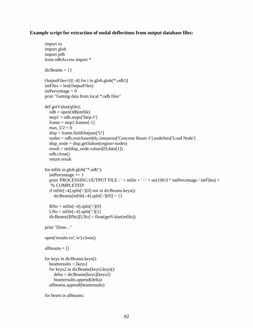
82

Example script for extraction of nodal deflections from output database files:

import os

import glob

import pdb

from odbAccess import *

dicBeams = {}

OutputFiles=[i[:-4] for i in glob.glob('*.odb')]

intFiles = len(OutputFiles)

intPercentage = 0

print "Getting data from local *.odb files"

def getValue(qfile):

odb = openOdb(mfile)

step1 = odb.steps['Step-1']

frame = step1.frames[-1]

max_U2 = 0

disp = frame.fieldOutputs['U']

nodes = odb.rootAssembly.instances['Concrete Beam-1'].nodeSets['Load Node']

disp_node = disp.getSubset(region=nodes)

result = str(disp_node.values[0].data[1])

odb.close()

return result

for mfile in glob.glob("*.odb"):

intPercentage += 1

print 'PROCESSING OUTPUT FILE : ' + mfile + ' - ' + str(100.0 * intPercentage / intFiles) +

'% COMPLETED'

if mfile[:-4].split('-')[0] not in dicBeams.keys():

dicBeams[mfile[:-4].split('-')[0]] = {}

BNo = mfile[:-4].split('-')[0]

LNo = mfile[:-4].split('-')[1]

dicBeams[BNo][LNo] = float(getValue(mfile))

print "Done..."

open('results.txt','w').close()

allbeams = []

for keys in dicBeams.keys():

beamresults = [keys]

for keys2 in dicBeams[keys].keys():

delta = dicBeams[keys][keys2]

beamresults.append(delta)

allbeams.append(beamresults)

for beam in allbeams:

83

for value in beam:

output = open('results.txt','a')

output.write(str(value))

output.write("\t")

output.close()

print "Writing beam " + str(beam[0]) + " to results.txt."

output = open('results.txt','a')

output.write("\n")

output.close()

print "Completed!"

print "Press Enter to end..."

raw_input()

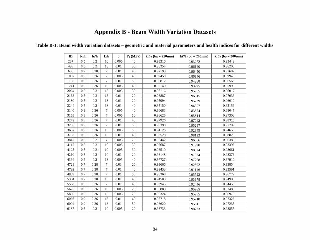
84

Appendix B - Beam Width Variation Datasets

Table B-1: Beam width variation datasets – geometric and material parameters and health indices for different widths

ID bw/h hs/h L/h ρ f'c (MPa) ki% (bw = 250mm) ki% (bw = 200mm) ki% (bw = 300mm)

287 0.5 0.2 10 0.005 40 0.93310 0.93272 0.93442

499 0.5 0.2 13 0.01 30 0.96354 0.96140 0.96200

685 0.7 0.28 7 0.01 40 0.97193 0.96450 0.97607

1087 0.9 0.36 7 0.005 40 0.89458 0.86946 0.89945

1186 0.9 0.36 7 0.01 50 0.95812 0.94368 0.96566

1241 0.9 0.36 10 0.005 40 0.95140 0.93995 0.95990

2064 0.5 0.2 13 0.005 30 0.96116 0.95965 0.96017

2168 0.5 0.2 13 0.01 20 0.96887 0.96915 0.97033

2180 0.5 0.2 13 0.01 20 0.95994 0.95739 0.96010

2244 0.5 0.2 13 0.01 40 0.95150 0.94857 0.95156

3140 0.9 0.36 7 0.005 40 0.86683 0.83874 0.88047

3153 0.9 0.36 7 0.005 50 0.96625 0.95814 0.97303

3242 0.9 0.36 7 0.01 40 0.97926 0.97042 0.98315

3285 0.9 0.36 7 0.01 50 0.96398 0.95297 0.97209

3667 0.9 0.36 13 0.005 50 0.94126 0.92845 0.94650

3753 0.9 0.36 13 0.01 40 0.98528 0.98122 0.98820

3847 0.5 0.2 7 0.005 20 0.96442 0.96066 0.96383

4112 0.5 0.2 10 0.005 30 0.92687 0.91990 0.92396

4125 0.5 0.2 10 0.005 30 0.98519 0.98324 0.98661

4210 0.5 0.2 10 0.01 20 0.98148 0.97824 0.98376

4394 0.5 0.2 13 0.005 40 0.97727 0.97268 0.97910

4728 0.7 0.28 7 0.01 20 0.93666 0.92502 0.93854

4792 0.7 0.28 7 0.01 40 0.92433 0.91146 0.92591

4809 0.7 0.28 7 0.01 50 0.96368 0.95523 0.96772

5304 0.7 0.28 13 0.01 40 0.94503 0.93978 0.94903

5568 0.9 0.36 7 0.01 40 0.93945 0.92446 0.94458

5625 0.9 0.36 10 0.005 20 0.96883 0.95965 0.97489

5866 0.9 0.36 13 0.005 20 0.96324 0.95255 0.96973

6066 0.9 0.36 13 0.01 40 0.96718 0.95710 0.97326

6094 0.9 0.36 13 0.01 50 0.96620 0.95611 0.97235

6187 0.5 0.2 10 0.005 20 0.98733 0.98723 0.98855

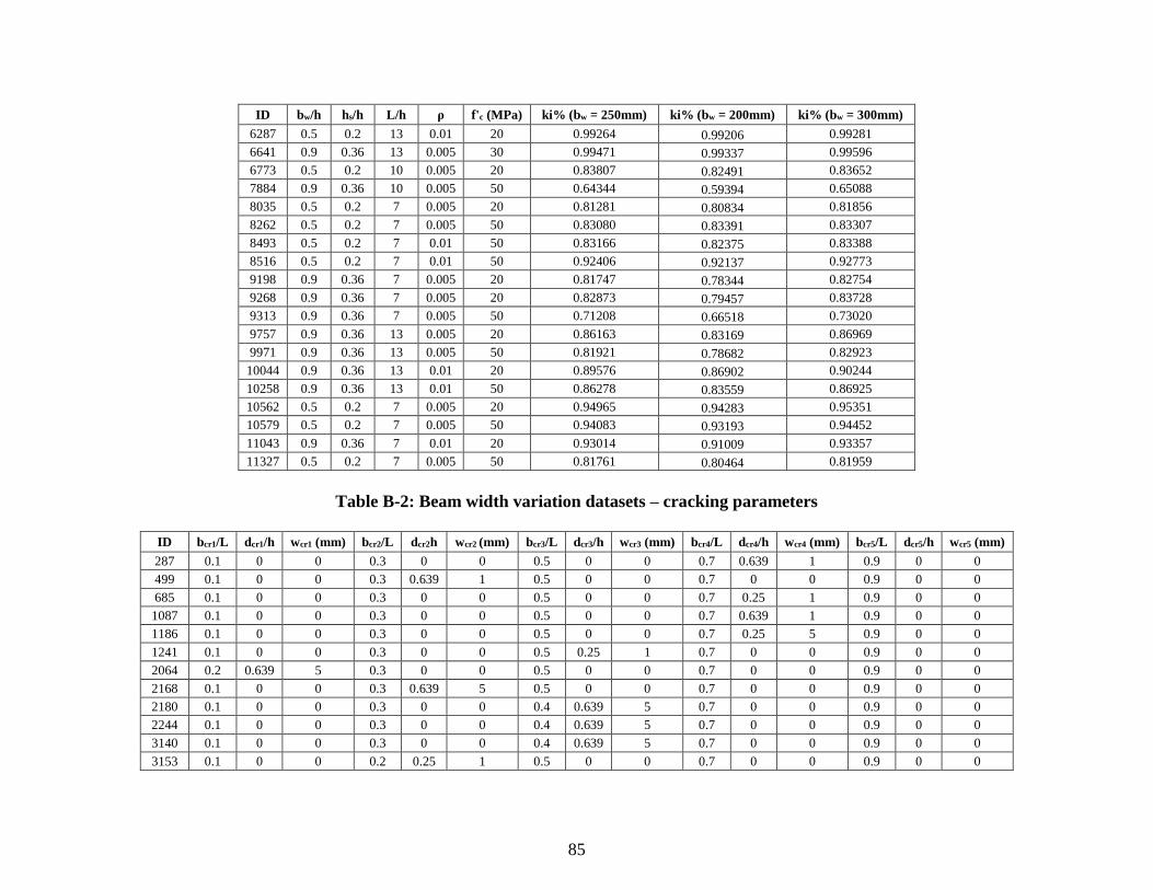
85

ID bw/h hs/h L/h ρ f'c (MPa) ki% (bw = 250mm) ki% (bw = 200mm) ki% (bw = 300mm)

6287 0.5 0.2 13 0.01 20 0.99264 0.99206 0.99281

6641 0.9 0.36 13 0.005 30 0.99471 0.99337 0.99596

6773 0.5 0.2 10 0.005 20 0.83807 0.82491 0.83652

7884 0.9 0.36 10 0.005 50 0.64344 0.59394 0.65088

8035 0.5 0.2 7 0.005 20 0.81281 0.80834 0.81856

8262 0.5 0.2 7 0.005 50 0.83080 0.83391 0.83307

8493 0.5 0.2 7 0.01 50 0.83166 0.82375 0.83388

8516 0.5 0.2 7 0.01 50 0.92406 0.92137 0.92773

9198 0.9 0.36 7 0.005 20 0.81747 0.78344 0.82754

9268 0.9 0.36 7 0.005 20 0.82873 0.79457 0.83728

9313 0.9 0.36 7 0.005 50 0.71208 0.66518 0.73020

9757 0.9 0.36 13 0.005 20 0.86163 0.83169 0.86969

9971 0.9 0.36 13 0.005 50 0.81921 0.78682 0.82923

10044 0.9 0.36 13 0.01 20 0.89576 0.86902 0.90244

10258 0.9 0.36 13 0.01 50 0.86278 0.83559 0.86925

10562 0.5 0.2 7 0.005 20 0.94965 0.94283 0.95351

10579 0.5 0.2 7 0.005 50 0.94083 0.93193 0.94452

11043 0.9 0.36 7 0.01 20 0.93014 0.91009 0.93357

11327 0.5 0.2 7 0.005 50 0.81761 0.80464 0.81959

Table B-2: Beam width variation datasets – cracking parameters

ID bcr1/L dcr1/h wcr1 (mm) bcr2/L dcr2h wcr2 (mm) bcr3/L dcr3/h wcr3 (mm) bcr4/L dcr4/h wcr4 (mm) bcr5/L dcr5/h wcr5 (mm)

287 0.1 0 0 0.3 0 0 0.5 0 0 0.7 0.639 1 0.9 0 0

499 0.1 0 0 0.3 0.639 1 0.5 0 0 0.7 0 0 0.9 0 0

685 0.1 0 0 0.3 0 0 0.5 0 0 0.7 0.25 1 0.9 0 0

1087 0.1 0 0 0.3 0 0 0.5 0 0 0.7 0.639 1 0.9 0 0

1186 0.1 0 0 0.3 0 0 0.5 0 0 0.7 0.25 5 0.9 0 0

1241 0.1 0 0 0.3 0 0 0.5 0.25 1 0.7 0 0 0.9 0 0

2064 0.2 0.639 5 0.3 0 0 0.5 0 0 0.7 0 0 0.9 0 0

2168 0.1 0 0 0.3 0.639 5 0.5 0 0 0.7 0 0 0.9 0 0

2180 0.1 0 0 0.3 0 0 0.4 0.639 5 0.7 0 0 0.9 0 0

2244 0.1 0 0 0.3 0 0 0.4 0.639 5 0.7 0 0 0.9 0 0

3140 0.1 0 0 0.3 0 0 0.4 0.639 5 0.7 0 0 0.9 0 0

3153 0.1 0 0 0.2 0.25 1 0.5 0 0 0.7 0 0 0.9 0 0

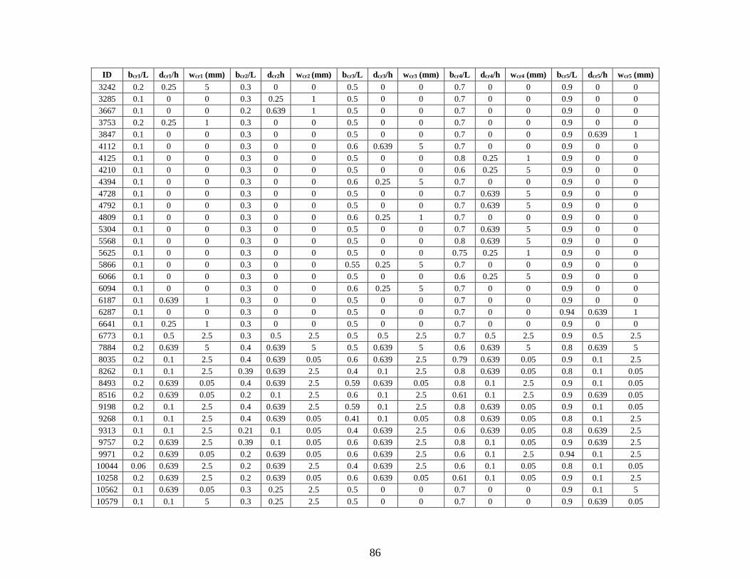
86

ID bcr1/L dcr1/h wcr1 (mm) bcr2/L dcr2h wcr2 (mm) bcr3/L dcr3/h wcr3 (mm) bcr4/L dcr4/h wcr4 (mm) bcr5/L dcr5/h wcr5 (mm)

3242 0.2 0.25 5 0.3 0 0 0.5 0 0 0.7 0 0 0.9 0 0

3285 0.1 0 0 0.3 0.25 1 0.5 0 0 0.7 0 0 0.9 0 0

3667 0.1 0 0 0.2 0.639 1 0.5 0 0 0.7 0 0 0.9 0 0

3753 0.2 0.25 1 0.3 0 0 0.5 0 0 0.7 0 0 0.9 0 0

3847 0.1 0 0 0.3 0 0 0.5 0 0 0.7 0 0 0.9 0.639 1

4112 0.1 0 0 0.3 0 0 0.6 0.639 5 0.7 0 0 0.9 0 0

4125 0.1 0 0 0.3 0 0 0.5 0 0 0.8 0.25 1 0.9 0 0

4210 0.1 0 0 0.3 0 0 0.5 0 0 0.6 0.25 5 0.9 0 0

4394 0.1 0 0 0.3 0 0 0.6 0.25 5 0.7 0 0 0.9 0 0

4728 0.1 0 0 0.3 0 0 0.5 0 0 0.7 0.639 5 0.9 0 0

4792 0.1 0 0 0.3 0 0 0.5 0 0 0.7 0.639 5 0.9 0 0

4809 0.1 0 0 0.3 0 0 0.6 0.25 1 0.7 0 0 0.9 0 0

5304 0.1 0 0 0.3 0 0 0.5 0 0 0.7 0.639 5 0.9 0 0

5568 0.1 0 0 0.3 0 0 0.5 0 0 0.8 0.639 5 0.9 0 0

5625 0.1 0 0 0.3 0 0 0.5 0 0 0.75 0.25 1 0.9 0 0

5866 0.1 0 0 0.3 0 0 0.55 0.25 5 0.7 0 0 0.9 0 0

6066 0.1 0 0 0.3 0 0 0.5 0 0 0.6 0.25 5 0.9 0 0

6094 0.1 0 0 0.3 0 0 0.6 0.25 5 0.7 0 0 0.9 0 0

6187 0.1 0.639 1 0.3 0 0 0.5 0 0 0.7 0 0 0.9 0 0

6287 0.1 0 0 0.3 0 0 0.5 0 0 0.7 0 0 0.94 0.639 1

6641 0.1 0.25 1 0.3 0 0 0.5 0 0 0.7 0 0 0.9 0 0

6773 0.1 0.5 2.5 0.3 0.5 2.5 0.5 0.5 2.5 0.7 0.5 2.5 0.9 0.5 2.5

7884 0.2 0.639 5 0.4 0.639 5 0.5 0.639 5 0.6 0.639 5 0.8 0.639 5

8035 0.2 0.1 2.5 0.4 0.639 0.05 0.6 0.639 2.5 0.79 0.639 0.05 0.9 0.1 2.5

8262 0.1 0.1 2.5 0.39 0.639 2.5 0.4 0.1 2.5 0.8 0.639 0.05 0.8 0.1 0.05

8493 0.2 0.639 0.05 0.4 0.639 2.5 0.59 0.639 0.05 0.8 0.1 2.5 0.9 0.1 0.05

8516 0.2 0.639 0.05 0.2 0.1 2.5 0.6 0.1 2.5 0.61 0.1 2.5 0.9 0.639 0.05

9198 0.2 0.1 2.5 0.4 0.639 2.5 0.59 0.1 2.5 0.8 0.639 0.05 0.9 0.1 0.05

9268 0.1 0.1 2.5 0.4 0.639 0.05 0.41 0.1 0.05 0.8 0.639 0.05 0.8 0.1 2.5

9313 0.1 0.1 2.5 0.21 0.1 0.05 0.4 0.639 2.5 0.6 0.639 0.05 0.8 0.639 2.5

9757 0.2 0.639 2.5 0.39 0.1 0.05 0.6 0.639 2.5 0.8 0.1 0.05 0.9 0.639 2.5

9971 0.2 0.639 0.05 0.2 0.639 0.05 0.6 0.639 2.5 0.6 0.1 2.5 0.94 0.1 2.5

10044 0.06 0.639 2.5 0.2 0.639 2.5 0.4 0.639 2.5 0.6 0.1 0.05 0.8 0.1 0.05

10258 0.2 0.639 2.5 0.2 0.639 0.05 0.6 0.639 0.05 0.61 0.1 0.05 0.9 0.1 2.5

10562 0.1 0.639 0.05 0.3 0.25 2.5 0.5 0 0 0.7 0 0 0.9 0.1 5

10579 0.1 0.1 5 0.3 0.25 2.5 0.5 0 0 0.7 0 0 0.9 0.639 0.05

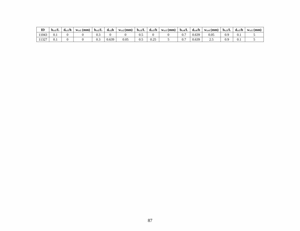
87

ID bcr1/L dcr1/h wcr1 (mm) bcr2/L dcr2h wcr2 (mm) bcr3/L dcr3/h wcr3 (mm) bcr4/L dcr4/h wcr4 (mm) bcr5/L dcr5/h wcr5 (mm)

11043 0.1 0 0 0.3 0 0 0.5 0 0 0.7 0.639 0.05 0.9 0.1 5

11327 0.1 0 0 0.3 0.639 0.05 0.5 0.25 5 0.7 0.639 2.5 0.9 0.1 5

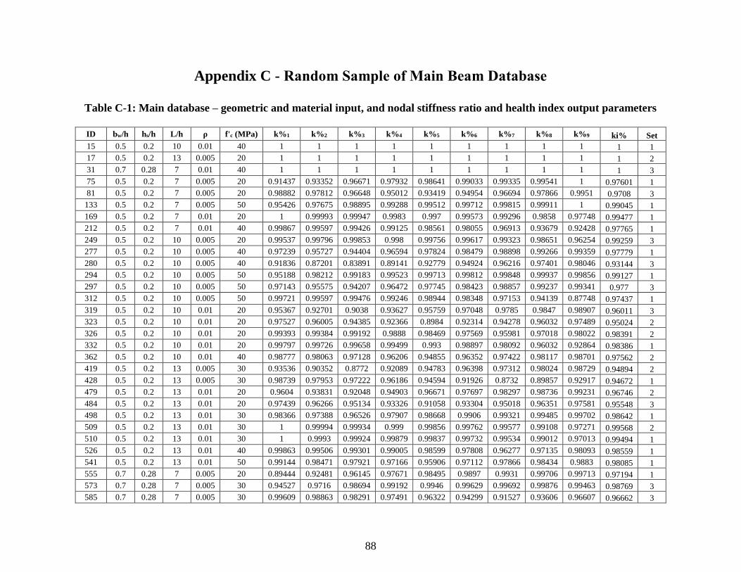
88

Appendix C - Random Sample of Main Beam Database

Table C-1: Main database – geometric and material input, and nodal stiffness ratio and health index output parameters

ID bw/h hs/h L/h ρ f'c (MPa) k%1 k%2 k%3 k%4 k%5 k%6 k%7 k%8 k%9 ki% Set

15 0.5 0.2 10 0.01 40 1 1 1 1 1 1 1 1 1 1 1

17 0.5 0.2 13 0.005 20 1 1 1 1 1 1 1 1 1 1 2

31 0.7 0.28 7 0.01 40 1 1 1 1 1 1 1 1 1 1 3

75 0.5 0.2 7 0.005 20 0.91437 0.93352 0.96671 0.97932 0.98641 0.99033 0.99335 0.99541 1 0.97601 1

81 0.5 0.2 7 0.005 20 0.98882 0.97812 0.96648 0.95012 0.93419 0.94954 0.96694 0.97866 0.9951 0.9708 3

133 0.5 0.2 7 0.005 50 0.95426 0.97675 0.98895 0.99288 0.99512 0.99712 0.99815 0.99911 1 0.99045 1

169 0.5 0.2 7 0.01 20 1 0.99993 0.99947 0.9983 0.997 0.99573 0.99296 0.9858 0.97748 0.99477 1

212 0.5 0.2 7 0.01 40 0.99867 0.99597 0.99426 0.99125 0.98561 0.98055 0.96913 0.93679 0.92428 0.97765 1

249 0.5 0.2 10 0.005 20 0.99537 0.99796 0.99853 0.998 0.99756 0.99617 0.99323 0.98651 0.96254 0.99259 3

277 0.5 0.2 10 0.005 40 0.97239 0.95727 0.94404 0.96594 0.97824 0.98479 0.98898 0.99266 0.99359 0.97779 1

280 0.5 0.2 10 0.005 40 0.91836 0.87201 0.83891 0.89141 0.92779 0.94924 0.96216 0.97401 0.98046 0.93144 3

294 0.5 0.2 10 0.005 50 0.95188 0.98212 0.99183 0.99523 0.99713 0.99812 0.99848 0.99937 0.99856 0.99127 1

297 0.5 0.2 10 0.005 50 0.97143 0.95575 0.94207 0.96472 0.97745 0.98423 0.98857 0.99237 0.99341 0.977 3

312 0.5 0.2 10 0.005 50 0.99721 0.99597 0.99476 0.99246 0.98944 0.98348 0.97153 0.94139 0.87748 0.97437 1

319 0.5 0.2 10 0.01 20 0.95367 0.92701 0.9038 0.93627 0.95759 0.97048 0.9785 0.9847 0.98907 0.96011 3

323 0.5 0.2 10 0.01 20 0.97527 0.96005 0.94385 0.92366 0.8984 0.92314 0.94278 0.96032 0.97489 0.95024 2

326 0.5 0.2 10 0.01 20 0.99393 0.99384 0.99192 0.9888 0.98469 0.97569 0.95981 0.97018 0.98022 0.98391 2

332 0.5 0.2 10 0.01 20 0.99797 0.99726 0.99658 0.99499 0.993 0.98897 0.98092 0.96032 0.92864 0.98386 1

362 0.5 0.2 10 0.01 40 0.98777 0.98063 0.97128 0.96206 0.94855 0.96352 0.97422 0.98117 0.98701 0.97562 2

419 0.5 0.2 13 0.005 30 0.93536 0.90352 0.8772 0.92089 0.94783 0.96398 0.97312 0.98024 0.98729 0.94894 2

428 0.5 0.2 13 0.005 30 0.98739 0.97953 0.97222 0.96186 0.94594 0.91926 0.8732 0.89857 0.92917 0.94672 1

479 0.5 0.2 13 0.01 20 0.9604 0.93831 0.92048 0.94903 0.96671 0.97697 0.98297 0.98736 0.99231 0.96746 2

484 0.5 0.2 13 0.01 20 0.97439 0.96266 0.95134 0.93326 0.91058 0.93304 0.95018 0.96351 0.97581 0.95548 3

498 0.5 0.2 13 0.01 30 0.98366 0.97388 0.96526 0.97907 0.98668 0.9906 0.99321 0.99485 0.99702 0.98642 1

509 0.5 0.2 13 0.01 30 1 0.99994 0.99934 0.999 0.99856 0.99762 0.99577 0.99108 0.97271 0.99568 2

510 0.5 0.2 13 0.01 30 1 0.9993 0.99924 0.99879 0.99837 0.99732 0.99534 0.99012 0.97013 0.99494 1

526 0.5 0.2 13 0.01 40 0.99863 0.99506 0.99301 0.99005 0.98599 0.97808 0.96277 0.97135 0.98093 0.98559 1

541 0.5 0.2 13 0.01 50 0.99144 0.98471 0.97921 0.97166 0.95906 0.97112 0.97866 0.98434 0.9883 0.98085 1

555 0.7 0.28 7 0.005 20 0.89444 0.92481 0.96145 0.97671 0.98495 0.9897 0.9931 0.99706 0.99713 0.97194 1

573 0.7 0.28 7 0.005 30 0.94527 0.9716 0.98694 0.99192 0.9946 0.99629 0.99692 0.99876 0.99463 0.98769 3

585 0.7 0.28 7 0.005 30 0.99609 0.98863 0.98291 0.97491 0.96322 0.94299 0.91527 0.93606 0.96607 0.96662 3

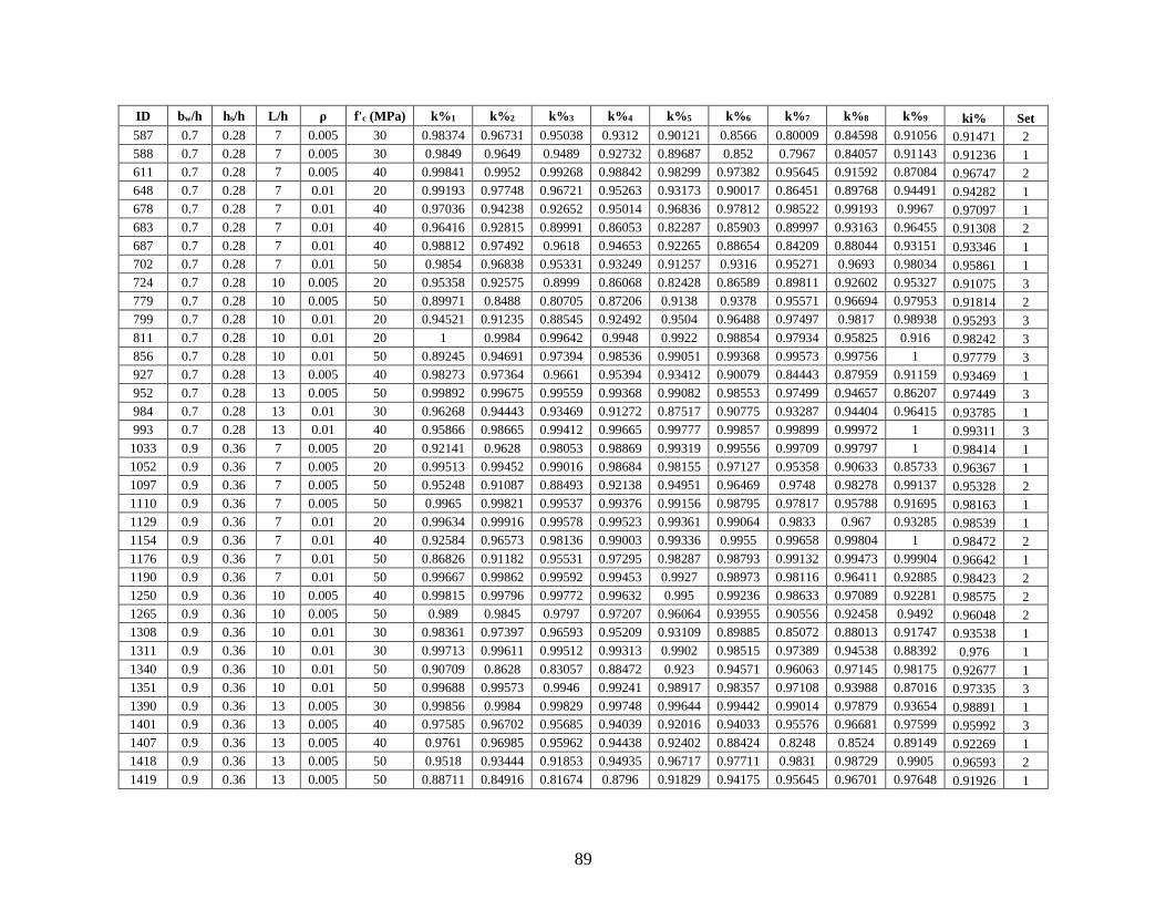
89

ID bw/h hs/h L/h ρ f'c (MPa) k%1 k%2 k%3 k%4 k%5 k%6 k%7 k%8 k%9 ki% Set

587 0.7 0.28 7 0.005 30 0.98374 0.96731 0.95038 0.9312 0.90121 0.8566 0.80009 0.84598 0.91056 0.91471 2

588 0.7 0.28 7 0.005 30 0.9849 0.9649 0.9489 0.92732 0.89687 0.852 0.7967 0.84057 0.91143 0.91236 1

611 0.7 0.28 7 0.005 40 0.99841 0.9952 0.99268 0.98842 0.98299 0.97382 0.95645 0.91592 0.87084 0.96747 2

648 0.7 0.28 7 0.01 20 0.99193 0.97748 0.96721 0.95263 0.93173 0.90017 0.86451 0.89768 0.94491 0.94282 1

678 0.7 0.28 7 0.01 40 0.97036 0.94238 0.92652 0.95014 0.96836 0.97812 0.98522 0.99193 0.9967 0.97097 1

683 0.7 0.28 7 0.01 40 0.96416 0.92815 0.89991 0.86053 0.82287 0.85903 0.89997 0.93163 0.96455 0.91308 2

687 0.7 0.28 7 0.01 40 0.98812 0.97492 0.9618 0.94653 0.92265 0.88654 0.84209 0.88044 0.93151 0.93346 1

702 0.7 0.28 7 0.01 50 0.9854 0.96838 0.95331 0.93249 0.91257 0.9316 0.95271 0.9693 0.98034 0.95861 1

724 0.7 0.28 10 0.005 20 0.95358 0.92575 0.8999 0.86068 0.82428 0.86589 0.89811 0.92602 0.95327 0.91075 3

779 0.7 0.28 10 0.005 50 0.89971 0.8488 0.80705 0.87206 0.9138 0.9378 0.95571 0.96694 0.97953 0.91814 2

799 0.7 0.28 10 0.01 20 0.94521 0.91235 0.88545 0.92492 0.9504 0.96488 0.97497 0.9817 0.98938 0.95293 3

811 0.7 0.28 10 0.01 20 1 0.9984 0.99642 0.9948 0.9922 0.98854 0.97934 0.95825 0.916 0.98242 3

856 0.7 0.28 10 0.01 50 0.89245 0.94691 0.97394 0.98536 0.99051 0.99368 0.99573 0.99756 1 0.97779 3

927 0.7 0.28 13 0.005 40 0.98273 0.97364 0.9661 0.95394 0.93412 0.90079 0.84443 0.87959 0.91159 0.93469 1

952 0.7 0.28 13 0.005 50 0.99892 0.99675 0.99559 0.99368 0.99082 0.98553 0.97499 0.94657 0.86207 0.97449 3

984 0.7 0.28 13 0.01 30 0.96268 0.94443 0.93469 0.91272 0.87517 0.90775 0.93287 0.94404 0.96415 0.93785 1

993 0.7 0.28 13 0.01 40 0.95866 0.98665 0.99412 0.99665 0.99777 0.99857 0.99899 0.99972 1 0.99311 3

1033 0.9 0.36 7 0.005 20 0.92141 0.9628 0.98053 0.98869 0.99319 0.99556 0.99709 0.99797 1 0.98414 1

1052 0.9 0.36 7 0.005 20 0.99513 0.99452 0.99016 0.98684 0.98155 0.97127 0.95358 0.90633 0.85733 0.96367 1

1097 0.9 0.36 7 0.005 50 0.95248 0.91087 0.88493 0.92138 0.94951 0.96469 0.9748 0.98278 0.99137 0.95328 2

1110 0.9 0.36 7 0.005 50 0.9965 0.99821 0.99537 0.99376 0.99156 0.98795 0.97817 0.95788 0.91695 0.98163 1

1129 0.9 0.36 7 0.01 20 0.99634 0.99916 0.99578 0.99523 0.99361 0.99064 0.9833 0.967 0.93285 0.98539 1

1154 0.9 0.36 7 0.01 40 0.92584 0.96573 0.98136 0.99003 0.99336 0.9955 0.99658 0.99804 1 0.98472 2

1176 0.9 0.36 7 0.01 50 0.86826 0.91182 0.95531 0.97295 0.98287 0.98793 0.99132 0.99473 0.99904 0.96642 1

1190 0.9 0.36 7 0.01 50 0.99667 0.99862 0.99592 0.99453 0.9927 0.98973 0.98116 0.96411 0.92885 0.98423 2

1250 0.9 0.36 10 0.005 40 0.99815 0.99796 0.99772 0.99632 0.995 0.99236 0.98633 0.97089 0.92281 0.98575 2

1265 0.9 0.36 10 0.005 50 0.989 0.9845 0.9797 0.97207 0.96064 0.93955 0.90556 0.92458 0.9492 0.96048 2

1308 0.9 0.36 10 0.01 30 0.98361 0.97397 0.96593 0.95209 0.93109 0.89885 0.85072 0.88013 0.91747 0.93538 1

1311 0.9 0.36 10 0.01 30 0.99713 0.99611 0.99512 0.99313 0.9902 0.98515 0.97389 0.94538 0.88392 0.976 1

1340 0.9 0.36 10 0.01 50 0.90709 0.8628 0.83057 0.88472 0.923 0.94571 0.96063 0.97145 0.98175 0.92677 1

1351 0.9 0.36 10 0.01 50 0.99688 0.99573 0.9946 0.99241 0.98917 0.98357 0.97108 0.93988 0.87016 0.97335 3

1390 0.9 0.36 13 0.005 30 0.99856 0.9984 0.99829 0.99748 0.99644 0.99442 0.99014 0.97879 0.93654 0.98891 1

1401 0.9 0.36 13 0.005 40 0.97585 0.96702 0.95685 0.94039 0.92016 0.94033 0.95576 0.96681 0.97599 0.95992 3

1407 0.9 0.36 13 0.005 40 0.9761 0.96985 0.95962 0.94438 0.92402 0.88424 0.8248 0.8524 0.89149 0.92269 1

1418 0.9 0.36 13 0.005 50 0.9518 0.93444 0.91853 0.94935 0.96717 0.97711 0.9831 0.98729 0.9905 0.96593 2

1419 0.9 0.36 13 0.005 50 0.88711 0.84916 0.81674 0.8796 0.91829 0.94175 0.95645 0.96701 0.97648 0.91926 1

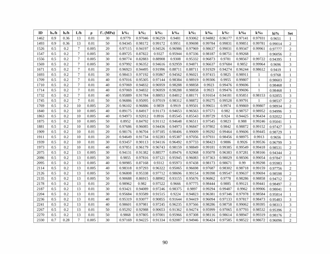
90

ID bw/h hs/h L/h ρ f'c (MPa) k%1 k%2 k%3 k%4 k%5 k%6 k%7 k%8 k%9 ki% Set

1462 0.9 0.36 13 0.01 30 0.9779 0.97046 0.96259 0.9481 0.93062 0.94882 0.96177 0.97141 0.97931 0.9651 1

1493 0.9 0.36 13 0.01 50 0.94345 0.98172 0.99172 0.9951 0.99698 0.99784 0.99831 0.99851 0.99781 0.99014 2

1526 0.5 0.2 7 0.005 20 0.97115 0.94197 0.94526 0.96986 0.97969 0.98637 0.99031 0.99347 0.99961 0.97777 2

1547 0.5 0.2 7 0.005 30 0.89725 0.87822 0.9327 0.95944 0.97336 0.98187 0.98751 0.99268 1 0.96056 2

1556 0.5 0.2 7 0.005 30 0.90774 0.82883 0.88908 0.9308 0.95332 0.96873 0.9781 0.98567 0.99722 0.94395 1

1569 0.5 0.2 7 0.005 30 0.97992 0.96352 0.94616 0.92959 0.94871 0.96637 0.97684 0.9852 0.99964 0.9696 3

1671 0.5 0.2 7 0.01 20 0.96923 0.94495 0.91996 0.88711 0.88711 0.91929 0.94274 0.96244 0.98612 0.9419 1

1693 0.5 0.2 7 0.01 30 0.98413 0.97192 0.95867 0.94562 0.96021 0.97415 0.9825 0.98911 1 0.9768 1

1709 0.5 0.2 7 0.01 40 0.97016 0.95305 0.97144 0.98384 0.98919 0.99306 0.9955 0.99807 1 0.98603 2

1710 0.5 0.2 7 0.01 40 0.97069 0.94832 0.96959 0.98288 0.98858 0.9923 0.99476 0.99696 1 0.98468 1

1714 0.5 0.2 7 0.01 40 0.97069 0.94832 0.96959 0.98288 0.98858 0.9923 0.99476 0.99696 1 0.98468 1

1732 0.5 0.2 7 0.01 40 0.95889 0.91784 0.88053 0.84812 0.88171 0.91654 0.94181 0.95851 0.98153 0.92855 3

1745 0.5 0.2 7 0.01 50 0.96886 0.95095 0.97019 0.98312 0.98872 0.99275 0.99528 0.99791 1 0.98537 2

1769 0.5 0.2 10 0.005 20 0.96102 0.96886 0.9859 0.9919 0.99501 0.99651 0.9974 0.99869 0.99807 0.98934 2

1840 0.5 0.2 10 0.005 40 0.89175 0.84917 0.91173 0.94653 0.96563 0.97571 0.982 0.98757 0.98952 0.94996 3

1863 0.5 0.2 10 0.005 40 0.94973 0.92012 0.8916 0.85545 0.85543 0.89729 0.924 0.94425 0.96434 0.92022 1

1875 0.5 0.2 10 0.005 50 0.8952 0.84792 0.91112 0.94648 0.96511 0.97545 0.9823 0.988 0.99246 0.95041 1

1881 0.5 0.2 10 0.005 50 0.97686 0.96085 0.94436 0.94973 0.96847 0.97802 0.9842 0.98872 0.99152 0.97427 3

1909 0.5 0.2 10 0.01 20 0.98176 0.96704 0.97185 0.98406 0.99009 0.99292 0.99464 0.99606 0.99445 0.98729 1

1911 0.5 0.2 10 0.01 20 0.94649 0.91734 0.92283 0.95387 0.97056 0.97931 0.98456 0.98975 0.9913 0.9656 1

1939 0.5 0.2 10 0.01 30 0.93457 0.90113 0.94116 0.96492 0.97733 0.98423 0.9886 0.9926 0.99536 0.96799 3

1973 0.5 0.2 10 0.01 40 0.97851 0.96179 0.96743 0.98159 0.98849 0.99181 0.99385 0.99549 0.99418 0.98531 2

2075 0.5 0.2 13 0.005 30 0.94131 0.91382 0.88577 0.89476 0.92968 0.95078 0.96383 0.97281 0.98166 0.94344 2

2086 0.5 0.2 13 0.005 30 0.9855 0.97816 0.97121 0.95945 0.96083 0.97363 0.98029 0.98506 0.99054 0.97847 1

2095 0.5 0.2 13 0.005 40 0.90985 0.87168 0.9312 0.95973 0.97438 0.98173 0.98671 0.99 0.99298 0.95983 3

2114 0.5 0.2 13 0.005 40 0.98318 0.97293 0.96322 0.95065 0.96698 0.97687 0.98302 0.98718 0.99159 0.97756 2

2126 0.5 0.2 13 0.005 50 0.96808 0.95338 0.97712 0.98696 0.99154 0.99398 0.99547 0.99637 0.99694 0.98598 2

2135 0.5 0.2 13 0.005 50 0.90688 0.86915 0.88902 0.93155 0.95676 0.96862 0.9778 0.98286 0.98858 0.94712 2

2178 0.5 0.2 13 0.01 20 0.98962 0.982 0.97522 0.9666 0.97775 0.98444 0.9885 0.99121 0.99441 0.98497 2

2187 0.5 0.2 13 0.01 30 0.93421 0.94089 0.97246 0.98375 0.9897 0.99294 0.99487 0.9962 0.99906 0.98041 1

2204 0.5 0.2 13 0.01 30 0.95684 0.93589 0.91515 0.9224 0.94823 0.96381 0.97346 0.97978 0.98584 0.95814 1

2236 0.5 0.2 13 0.01 40 0.95319 0.93077 0.90855 0.91644 0.94419 0.96094 0.97133 0.97817 0.98473 0.95483 3

2241 0.5 0.2 13 0.01 40 0.98601 0.97981 0.97245 0.96235 0.97566 0.98286 0.98758 0.99062 0.99395 0.98313 3

2267 0.5 0.2 13 0.01 50 0.95292 0.92988 0.90653 0.91362 0.94274 0.95999 0.97065 0.97793 0.98532 0.95396 2

2270 0.5 0.2 13 0.01 50 0.9868 0.97805 0.97001 0.95966 0.97308 0.98116 0.98614 0.98947 0.99319 0.98176 2

2330 0.7 0.28 7 0.005 30 0.97169 0.94225 0.91334 0.92087 0.94946 0.96424 0.97585 0.98522 0.98672 0.96096 2

91

ID bw/h hs/h L/h ρ f'c (MPa) k%1 k%2 k%3 k%4 k%5 k%6 k%7 k%8 k%9 ki% Set

2358 0.7 0.28 7 0.005 40 0.96115 0.91953 0.92722 0.95732 0.97239 0.98099 0.98695 0.99244 0.9945 0.96925 1

2359 0.7 0.28 7 0.005 40 0.8986 0.81043 0.82422 0.88597 0.92464 0.94566 0.96179 0.97602 0.98853 0.92159 3

2371 0.7 0.28 7 0.005 40 0.92805 0.86828 0.81703 0.77408 0.8255 0.87445 0.90954 0.93853 0.96868 0.89041 3

2396 0.7 0.28 7 0.005 50 0.91284 0.84056 0.78101 0.79401 0.85268 0.89459 0.92276 0.94846 0.97225 0.89192 1

2402 0.7 0.28 7 0.005 50 0.97109 0.94748 0.92252 0.90081 0.92758 0.95055 0.96568 0.97805 0.98782 0.95516 2

2429 0.7 0.28 7 0.01 20 0.98483 0.96489 0.94709 0.9313 0.9502 0.96666 0.97741 0.98582 0.99046 0.96987 2

2435 0.7 0.28 7 0.01 20 0.95736 0.92017 0.88659 0.85809 0.89104 0.92311 0.94555 0.96429 0.98276 0.9329 2

2459 0.7 0.28 7 0.01 30 0.95029 0.90324 0.85991 0.86348 0.90734 0.93432 0.95303 0.96959 0.98418 0.93254 2

2465 0.7 0.28 7 0.01 30 0.98321 0.96202 0.94294 0.92612 0.94641 0.96404 0.97552 0.98447 0.98978 0.96745 2

2482 0.7 0.28 7 0.01 40 0.95701 0.93359 0.96015 0.97709 0.98485 0.98934 0.9927 0.99571 0.99427 0.97847 1

2508 0.7 0.28 7 0.01 50 0.89618 0.87549 0.93226 0.95836 0.97298 0.9813 0.9881 0.99444 0.99899 0.95981 1

2546 0.7 0.28 10 0.005 20 0.95728 0.93546 0.96598 0.98054 0.98738 0.99159 0.99383 0.99645 0.99988 0.98084 2

2569 0.7 0.28 10 0.005 30 0.94915 0.9578 0.98061 0.98879 0.99295 0.99539 0.99648 0.99833 1 0.98612 1

2596 0.7 0.28 10 0.005 30 0.93147 0.89196 0.85934 0.82259 0.86825 0.90552 0.93172 0.95138 0.9701 0.91323 3

2601 0.7 0.28 10 0.005 40 0.94687 0.95607 0.9798 0.98833 0.99265 0.99518 0.99633 0.99821 1 0.9855 3

2604 0.7 0.28 10 0.005 40 0.86407 0.87533 0.93652 0.96318 0.97574 0.98348 0.98785 0.99194 0.9968 0.95749 1

2612 0.7 0.28 10 0.005 40 0.87527 0.82232 0.89556 0.93816 0.95917 0.97121 0.97897 0.98549 0.99275 0.94189 1

2683 0.7 0.28 10 0.01 20 0.95244 0.92386 0.89474 0.90342 0.9344 0.9549 0.96663 0.97705 0.98742 0.94949 3

2692 0.7 0.28 10 0.01 20 0.95765 0.93112 0.90795 0.88256 0.91387 0.93922 0.9566 0.96965 0.98257 0.94412 3

2733 0.7 0.28 10 0.01 40 0.96228 0.94424 0.97142 0.98284 0.98927 0.99281 0.9946 0.99695 0.9998 0.98342 3

2746 0.7 0.28 10 0.01 40 0.97724 0.96034 0.94169 0.94751 0.9665 0.97721 0.98318 0.9892 0.99678 0.97397 1

2779 0.7 0.28 10 0.01 50 0.93805 0.90301 0.86741 0.87919 0.9173 0.94278 0.95737 0.97015 0.98284 0.93581 3

2780 0.7 0.28 10 0.01 50 0.9375 0.89909 0.8664 0.87527 0.91473 0.93992 0.9557 0.9694 0.98455 0.93426 1

2784 0.7 0.28 10 0.01 50 0.94496 0.91207 0.88413 0.85299 0.89162 0.92289 0.94461 0.96087 0.97659 0.92907 1

2795 0.7 0.28 13 0.005 20 0.88977 0.9116 0.95719 0.97547 0.98441 0.98915 0.99187 0.99452 0.99505 0.9689 2

2798 0.7 0.28 13 0.005 20 0.9601 0.94481 0.97276 0.98448 0.98993 0.9931 0.9949 0.99672 0.99717 0.9834 2

2812 0.7 0.28 13 0.005 20 0.93117 0.90195 0.87142 0.8795 0.91953 0.94406 0.95807 0.96819 0.97822 0.93521 3

2815 0.7 0.28 13 0.005 20 0.94496 0.92231 0.89537 0.86684 0.90668 0.93415 0.95091 0.96393 0.97462 0.93598 3

2856 0.7 0.28 13 0.005 30 0.94663 0.92267 0.89791 0.86479 0.87049 0.90563 0.93048 0.9468 0.96354 0.92489 1

2913 0.7 0.28 13 0.005 50 0.97596 0.96457 0.95217 0.93765 0.95721 0.97035 0.97833 0.9842 0.98946 0.97099 3

2921 0.7 0.28 13 0.01 20 0.96453 0.97343 0.98814 0.99322 0.99578 0.99708 0.99795 0.99901 0.99952 0.99087 2

2925 0.7 0.28 13 0.01 20 0.96863 0.95711 0.97939 0.98822 0.99221 0.99468 0.99616 0.99762 0.99841 0.98724 3

2931 0.7 0.28 13 0.01 20 0.93171 0.90795 0.95056 0.97135 0.98126 0.98706 0.99058 0.99352 0.99551 0.97095 1

2954 0.7 0.28 13 0.01 30 0.9595 0.9702 0.9868 0.99243 0.99505 0.99664 0.99751 0.99864 0.99874 0.98955 2

2996 0.7 0.28 13 0.01 40 0.91527 0.88699 0.93908 0.96411 0.97705 0.98406 0.98804 0.99213 0.99501 0.96417 1

3049 0.9 0.36 7 0.005 20 0.93208 0.93482 0.96734 0.98048 0.98716 0.99172 0.99391 0.99484 0.99586 0.97782 1

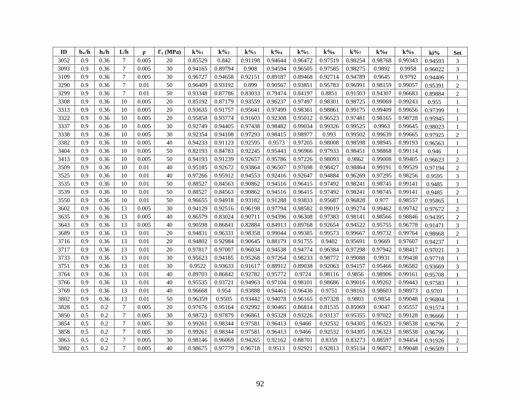
92

ID bw/h hs/h L/h ρ f'c (MPa) k%1 k%2 k%3 k%4 k%5 k%6 k%7 k%8 k%9 ki% Set

3052 0.9 0.36 7 0.005 20 0.85529 0.842 0.91198 0.94644 0.96472 0.97519 0.98254 0.98768 0.99343 0.94593 3

3093 0.9 0.36 7 0.005 30 0.94165 0.89794 0.908 0.94594 0.96505 0.97585 0.98275 0.9892 0.9958 0.96022 3

3109 0.9 0.36 7 0.005 30 0.96727 0.94658 0.92151 0.89187 0.89468 0.92714 0.94789 0.9645 0.9792 0.94406 1

3290 0.9 0.36 7 0.01 50 0.96409 0.93192 0.899 0.90567 0.93851 0.95783 0.96991 0.98159 0.99057 0.95391 2

3299 0.9 0.36 7 0.01 50 0.93348 0.87786 0.83033 0.79474 0.84197 0.8851 0.91503 0.94307 0.96683 0.89884 2

3308 0.9 0.36 10 0.005 20 0.85192 0.87179 0.93559 0.96237 0.97497 0.98301 0.98725 0.99069 0.99243 0.955 1

3313 0.9 0.36 10 0.005 20 0.93635 0.91757 0.95641 0.97499 0.98361 0.98861 0.99175 0.99409 0.99656 0.97399 1

3322 0.9 0.36 10 0.005 20 0.95858 0.93774 0.91603 0.92308 0.95012 0.96523 0.97481 0.98165 0.98728 0.95945 1

3337 0.9 0.36 10 0.005 30 0.92749 0.94405 0.97438 0.98482 0.99034 0.99326 0.99525 0.9963 0.99645 0.98023 1

3338 0.9 0.36 10 0.005 30 0.92354 0.94108 0.97293 0.98415 0.98977 0.993 0.99502 0.99639 0.99665 0.97925 2

3382 0.9 0.36 10 0.005 40 0.94233 0.91123 0.92595 0.9573 0.97205 0.98008 0.98598 0.98945 0.99193 0.96563 1

3404 0.9 0.36 10 0.005 50 0.82193 0.84783 0.92245 0.95443 0.96966 0.97933 0.98451 0.98868 0.99114 0.946 1

3413 0.9 0.36 10 0.005 50 0.94193 0.91239 0.92657 0.95786 0.97226 0.98093 0.9862 0.99008 0.99405 0.96623 2

3509 0.9 0.36 10 0.01 40 0.95185 0.92672 0.93864 0.96507 0.97698 0.98427 0.98864 0.99191 0.99529 0.97194 2

3525 0.9 0.36 10 0.01 40 0.97266 0.95912 0.94553 0.92416 0.92647 0.94884 0.96269 0.97295 0.98256 0.9595 3

3535 0.9 0.36 10 0.01 50 0.88527 0.84563 0.90862 0.94516 0.96415 0.97492 0.98241 0.98745 0.99141 0.9485 3

3539 0.9 0.36 10 0.01 50 0.88527 0.84563 0.90862 0.94516 0.96415 0.97492 0.98241 0.98745 0.99141 0.9485 2

3550 0.9 0.36 10 0.01 50 0.96655 0.94918 0.93182 0.91288 0.93833 0.95687 0.96828 0.977 0.98557 0.95865 1

3602 0.9 0.36 13 0.005 30 0.94129 0.92516 0.96198 0.97794 0.98582 0.99019 0.99274 0.99462 0.99742 0.97672 2

3635 0.9 0.36 13 0.005 40 0.86579 0.83024 0.90711 0.94396 0.96308 0.97383 0.98141 0.98566 0.98846 0.94395 2

3643 0.9 0.36 13 0.005 40 0.90598 0.86841 0.82884 0.84913 0.89768 0.92654 0.94522 0.95755 0.96778 0.91471 3

3689 0.9 0.36 13 0.01 20 0.94831 0.96331 0.98358 0.99044 0.99385 0.99573 0.99667 0.99732 0.99764 0.98668 2

3716 0.9 0.36 13 0.01 20 0.94802 0.92984 0.90645 0.88179 0.91755 0.9402 0.95691 0.9669 0.97607 0.94237 1

3717 0.9 0.36 13 0.01 20 0.97817 0.97007 0.96034 0.94538 0.94774 0.96384 0.97298 0.97942 0.98417 0.97021 3

3733 0.9 0.36 13 0.01 30 0.95623 0.94185 0.95268 0.97264 0.98233 0.98772 0.99088 0.9931 0.99438 0.97718 1

3751 0.9 0.36 13 0.01 30 0.9522 0.93633 0.91617 0.88912 0.89038 0.92063 0.94157 0.95466 0.96582 0.93669 3

3764 0.9 0.36 13 0.01 40 0.89703 0.86842 0.92782 0.95772 0.9724 0.98116 0.9856 0.98906 0.99161 0.95708 1

3766 0.9 0.36 13 0.01 40 0.95535 0.93721 0.94963 0.97104 0.98101 0.98686 0.99016 0.99262 0.99443 0.97583 1

3769 0.9 0.36 13 0.01 40 0.96668 0.954 0.93888 0.94461 0.96436 0.9751 0.98163 0.98603 0.98973 0.9701 1

3802 0.9 0.36 13 0.01 50 0.96359 0.9505 0.93442 0.94078 0.96165 0.97328 0.9803 0.9854 0.99048 0.96804 1

3828 0.5 0.2 7 0.005 20 0.97676 0.95164 0.92992 0.90465 0.86814 0.81535 0.85069 0.9047 0.95557 0.91574 1

3850 0.5 0.2 7 0.005 30 0.98723 0.97879 0.96861 0.95328 0.93226 0.93137 0.95355 0.97022 0.99128 0.96666 1

3854 0.5 0.2 7 0.005 30 0.99261 0.98344 0.97581 0.96413 0.9466 0.92532 0.94305 0.96323 0.98538 0.96796 2

3858 0.5 0.2 7 0.005 30 0.99261 0.98344 0.97581 0.96413 0.9466 0.92532 0.94305 0.96323 0.98538 0.96796 1

3863 0.5 0.2 7 0.005 30 0.98146 0.96069 0.94265 0.92162 0.88701 0.8359 0.83273 0.88597 0.94454 0.91926 2

3882 0.5 0.2 7 0.005 40 0.98675 0.97779 0.96718 0.9513 0.92921 0.92813 0.95134 0.96872 0.99048 0.96509 1

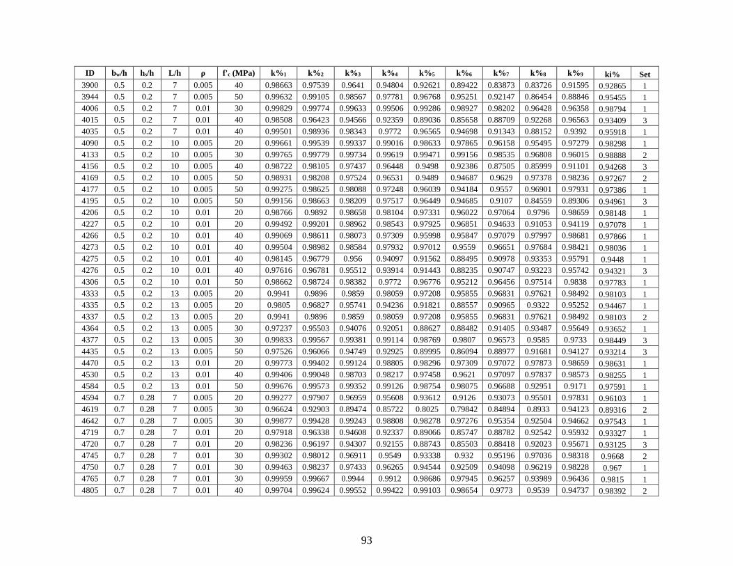
93

ID bw/h hs/h L/h ρ f'c (MPa) k%1 k%2 k%3 k%4 k%5 k%6 k%7 k%8 k%9 ki% Set

3900 0.5 0.2 7 0.005 40 0.98663 0.97539 0.9641 0.94804 0.92621 0.89422 0.83873 0.83726 0.91595 0.92865 1

3944 0.5 0.2 7 0.005 50 0.99632 0.99105 0.98567 0.97781 0.96768 0.95251 0.92147 0.86454 0.88846 0.95455 1

4006 0.5 0.2 7 0.01 30 0.99829 0.99774 0.99633 0.99506 0.99286 0.98927 0.98202 0.96428 0.96358 0.98794 1

4015 0.5 0.2 7 0.01 40 0.98508 0.96423 0.94566 0.92359 0.89036 0.85658 0.88709 0.92268 0.96563 0.93409 3

4035 0.5 0.2 7 0.01 40 0.99501 0.98936 0.98343 0.9772 0.96565 0.94698 0.91343 0.88152 0.9392 0.95918 1

4090 0.5 0.2 10 0.005 20 0.99661 0.99539 0.99337 0.99016 0.98633 0.97865 0.96158 0.95495 0.97279 0.98298 1

4133 0.5 0.2 10 0.005 30 0.99765 0.99779 0.99734 0.99619 0.99471 0.99156 0.98535 0.96808 0.96015 0.98888 2

4156 0.5 0.2 10 0.005 40 0.98722 0.98105 0.97437 0.96448 0.9498 0.92386 0.87505 0.85999 0.91101 0.94268 3

4169 0.5 0.2 10 0.005 50 0.98931 0.98208 0.97524 0.96531 0.9489 0.94687 0.9629 0.97378 0.98236 0.97267 2

4177 0.5 0.2 10 0.005 50 0.99275 0.98625 0.98088 0.97248 0.96039 0.94184 0.9557 0.96901 0.97931 0.97386 1

4195 0.5 0.2 10 0.005 50 0.99156 0.98663 0.98209 0.97517 0.96449 0.94685 0.9107 0.84559 0.89306 0.94961 3

4206 0.5 0.2 10 0.01 20 0.98766 0.9892 0.98658 0.98104 0.97331 0.96022 0.97064 0.9796 0.98659 0.98148 1

4227 0.5 0.2 10 0.01 20 0.99492 0.99201 0.98962 0.98543 0.97925 0.96851 0.94633 0.91053 0.94119 0.97078 1

4266 0.5 0.2 10 0.01 40 0.99069 0.98611 0.98073 0.97309 0.95998 0.95847 0.97079 0.97997 0.98681 0.97866 1

4273 0.5 0.2 10 0.01 40 0.99504 0.98982 0.98584 0.97932 0.97012 0.9559 0.96651 0.97684 0.98421 0.98036 1

4275 0.5 0.2 10 0.01 40 0.98145 0.96779 0.956 0.94097 0.91562 0.88495 0.90978 0.93353 0.95791 0.9448 1

4276 0.5 0.2 10 0.01 40 0.97616 0.96781 0.95512 0.93914 0.91443 0.88235 0.90747 0.93223 0.95742 0.94321 3

4306 0.5 0.2 10 0.01 50 0.98662 0.98724 0.98382 0.9772 0.96776 0.95212 0.96456 0.97514 0.9838 0.97783 1

4333 0.5 0.2 13 0.005 20 0.9941 0.9896 0.9859 0.98059 0.97208 0.95855 0.96831 0.97621 0.98492 0.98103 1

4335 0.5 0.2 13 0.005 20 0.9805 0.96827 0.95741 0.94236 0.91821 0.88557 0.90965 0.9322 0.95252 0.94467 1

4337 0.5 0.2 13 0.005 20 0.9941 0.9896 0.9859 0.98059 0.97208 0.95855 0.96831 0.97621 0.98492 0.98103 2

4364 0.5 0.2 13 0.005 30 0.97237 0.95503 0.94076 0.92051 0.88627 0.88482 0.91405 0.93487 0.95649 0.93652 1

4377 0.5 0.2 13 0.005 30 0.99833 0.99567 0.99381 0.99114 0.98769 0.9807 0.96573 0.9585 0.9733 0.98449 3

4435 0.5 0.2 13 0.005 50 0.97526 0.96066 0.94749 0.92925 0.89995 0.86094 0.88977 0.91681 0.94127 0.93214 3

4470 0.5 0.2 13 0.01 20 0.99773 0.99402 0.99124 0.98805 0.98296 0.97309 0.97072 0.97873 0.98659 0.98631 1

4530 0.5 0.2 13 0.01 40 0.99406 0.99048 0.98703 0.98217 0.97458 0.9621 0.97097 0.97837 0.98573 0.98255 1

4584 0.5 0.2 13 0.01 50 0.99676 0.99573 0.99352 0.99126 0.98754 0.98075 0.96688 0.92951 0.9171 0.97591 1

4594 0.7 0.28 7 0.005 20 0.99277 0.97907 0.96959 0.95608 0.93612 0.9126 0.93073 0.95501 0.97831 0.96103 1

4619 0.7 0.28 7 0.005 30 0.96624 0.92903 0.89474 0.85722 0.8025 0.79842 0.84894 0.8933 0.94123 0.89316 2

4642 0.7 0.28 7 0.005 30 0.99877 0.99428 0.99243 0.98808 0.98278 0.97276 0.95354 0.92504 0.94662 0.97543 1

4719 0.7 0.28 7 0.01 20 0.97918 0.96338 0.94608 0.92337 0.89066 0.85747 0.88782 0.92542 0.95932 0.93327 1

4720 0.7 0.28 7 0.01 20 0.98236 0.96197 0.94307 0.92155 0.88743 0.85503 0.88418 0.92023 0.95671 0.93125 3

4745 0.7 0.28 7 0.01 30 0.99302 0.98012 0.96911 0.9549 0.93338 0.932 0.95196 0.97036 0.98318 0.9668 2

4750 0.7 0.28 7 0.01 30 0.99463 0.98237 0.97433 0.96265 0.94544 0.92509 0.94098 0.96219 0.98228 0.967 1

4765 0.7 0.28 7 0.01 30 0.99959 0.99667 0.9944 0.9912 0.98686 0.97945 0.96257 0.93989 0.96436 0.9815 1

4805 0.7 0.28 7 0.01 40 0.99704 0.99624 0.99552 0.99422 0.99103 0.98654 0.9773 0.9539 0.94737 0.98392 2

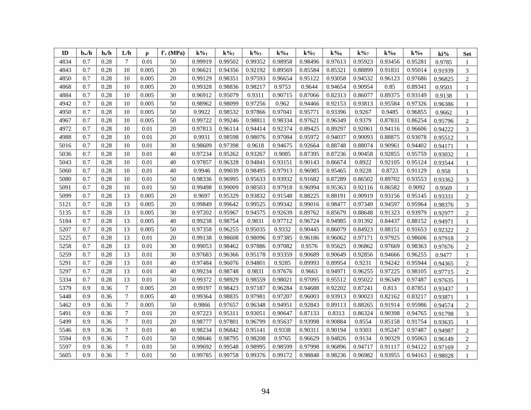
94

ID bw/h hs/h L/h ρ f'c (MPa) k%1 k%2 k%3 k%4 k%5 k%6 k%7 k%8 k%9 ki% Set

4834 0.7 0.28 7 0.01 50 0.99919 0.99502 0.99352 0.98958 0.98496 0.97613 0.95923 0.93456 0.95281 0.9785 1

4843 0.7 0.28 10 0.005 20 0.96621 0.94356 0.92192 0.89569 0.85584 0.85321 0.88899 0.91831 0.95014 0.91939 3

4850 0.7 0.28 10 0.005 20 0.99129 0.98351 0.97593 0.96654 0.95122 0.93058 0.94532 0.96123 0.97686 0.96825 2

4868 0.7 0.28 10 0.005 20 0.99328 0.98836 0.98217 0.9753 0.9644 0.94654 0.90954 0.85 0.89341 0.9503 1

4884 0.7 0.28 10 0.005 30 0.96912 0.95079 0.9311 0.90715 0.87066 0.82313 0.86077 0.89375 0.93149 0.9138 1

4942 0.7 0.28 10 0.005 50 0.98962 0.98099 0.97256 0.962 0.94466 0.92153 0.93813 0.95584 0.97326 0.96386 1

4950 0.7 0.28 10 0.005 50 0.9922 0.98532 0.97866 0.97041 0.95771 0.93396 0.9267 0.9485 0.96855 0.9662 1

4967 0.7 0.28 10 0.005 50 0.99722 0.99246 0.98811 0.98334 0.97621 0.96349 0.9379 0.87831 0.86254 0.95796 2

4972 0.7 0.28 10 0.01 20 0.97813 0.96114 0.94414 0.92374 0.89425 0.89297 0.92061 0.94116 0.96606 0.94222 3

4988 0.7 0.28 10 0.01 20 0.9931 0.98598 0.98076 0.97084 0.95972 0.94037 0.90093 0.88875 0.93078 0.95512 1

5016 0.7 0.28 10 0.01 30 0.98609 0.97398 0.9618 0.94675 0.92664 0.88748 0.88074 0.90961 0.94402 0.94171 1

5036 0.7 0.28 10 0.01 40 0.97234 0.95262 0.93267 0.9085 0.87395 0.87236 0.90458 0.92855 0.95759 0.93032 1

5043 0.7 0.28 10 0.01 40 0.97857 0.96328 0.94841 0.93151 0.90143 0.86674 0.8922 0.92105 0.95124 0.93544 1

5060 0.7 0.28 10 0.01 40 0.9946 0.99039 0.98495 0.97913 0.96985 0.95465 0.9228 0.8723 0.91129 0.958 1

5080 0.7 0.28 10 0.01 50 0.98336 0.96995 0.95633 0.93932 0.91682 0.87289 0.86502 0.89702 0.93553 0.93362 3

5091 0.7 0.28 10 0.01 50 0.99498 0.99009 0.98503 0.97918 0.96994 0.95363 0.92116 0.86582 0.9092 0.9569 1

5099 0.7 0.28 13 0.005 20 0.9697 0.95329 0.93832 0.91548 0.88225 0.88191 0.90919 0.93156 0.95145 0.93331 2

5121 0.7 0.28 13 0.005 20 0.99849 0.99642 0.99525 0.99342 0.99016 0.98477 0.97349 0.94597 0.95964 0.98376 3

5135 0.7 0.28 13 0.005 30 0.97202 0.95967 0.94575 0.92639 0.89762 0.85679 0.88648 0.91323 0.93979 0.92977 2

5184 0.7 0.28 13 0.005 40 0.99238 0.98754 0.9831 0.97712 0.96724 0.94985 0.91392 0.84437 0.88152 0.94971 1

5207 0.7 0.28 13 0.005 50 0.97358 0.96255 0.95035 0.9332 0.90445 0.86079 0.84923 0.88151 0.91653 0.92322 2

5225 0.7 0.28 13 0.01 20 0.99138 0.98608 0.98096 0.97385 0.96186 0.96062 0.97171 0.97925 0.98606 0.97918 2

5258 0.7 0.28 13 0.01 30 0.99053 0.98462 0.97886 0.97082 0.9576 0.95625 0.96862 0.97669 0.98363 0.97676 2

5259 0.7 0.28 13 0.01 30 0.97683 0.96366 0.95178 0.93359 0.90689 0.90649 0.92856 0.94666 0.96255 0.9477 1

5291 0.7 0.28 13 0.01 40 0.97484 0.96076 0.94801 0.9285 0.89993 0.89954 0.9231 0.94242 0.95944 0.94365 2

5297 0.7 0.28 13 0.01 40 0.99234 0.98748 0.9831 0.97676 0.9663 0.94971 0.96255 0.97225 0.98105 0.97715 2

5334 0.7 0.28 13 0.01 50 0.99372 0.98929 0.98559 0.98021 0.97095 0.95512 0.95022 0.96349 0.97487 0.97635 1

5379 0.9 0.36 7 0.005 20 0.99197 0.98423 0.97187 0.96284 0.94688 0.92202 0.87241 0.813 0.87851 0.93437 1

5448 0.9 0.36 7 0.005 40 0.99364 0.98835 0.97981 0.97207 0.96003 0.93913 0.90023 0.82162 0.83217 0.93871 1

5462 0.9 0.36 7 0.005 50 0.9866 0.97657 0.96348 0.94951 0.92843 0.89113 0.88265 0.91914 0.95986 0.94574 2

5491 0.9 0.36 7 0.01 20 0.97223 0.95311 0.93051 0.90647 0.87133 0.8313 0.86324 0.90398 0.94765 0.91798 3

5499 0.9 0.36 7 0.01 20 0.98777 0.97801 0.96799 0.95637 0.93998 0.90884 0.8554 0.85158 0.91754 0.93635 1

5546 0.9 0.36 7 0.01 40 0.98234 0.96842 0.95141 0.9338 0.90311 0.90194 0.9303 0.95247 0.97487 0.94987 2

5594 0.9 0.36 7 0.01 50 0.98646 0.98795 0.98208 0.9765 0.96629 0.94826 0.9134 0.90329 0.95063 0.96149 2

5597 0.9 0.36 7 0.01 50 0.99692 0.99548 0.98995 0.98599 0.97998 0.96896 0.94717 0.91117 0.94122 0.97169 2

5605 0.9 0.36 7 0.01 50 0.99785 0.99758 0.99376 0.99172 0.98848 0.98236 0.96982 0.93955 0.94163 0.98028 1

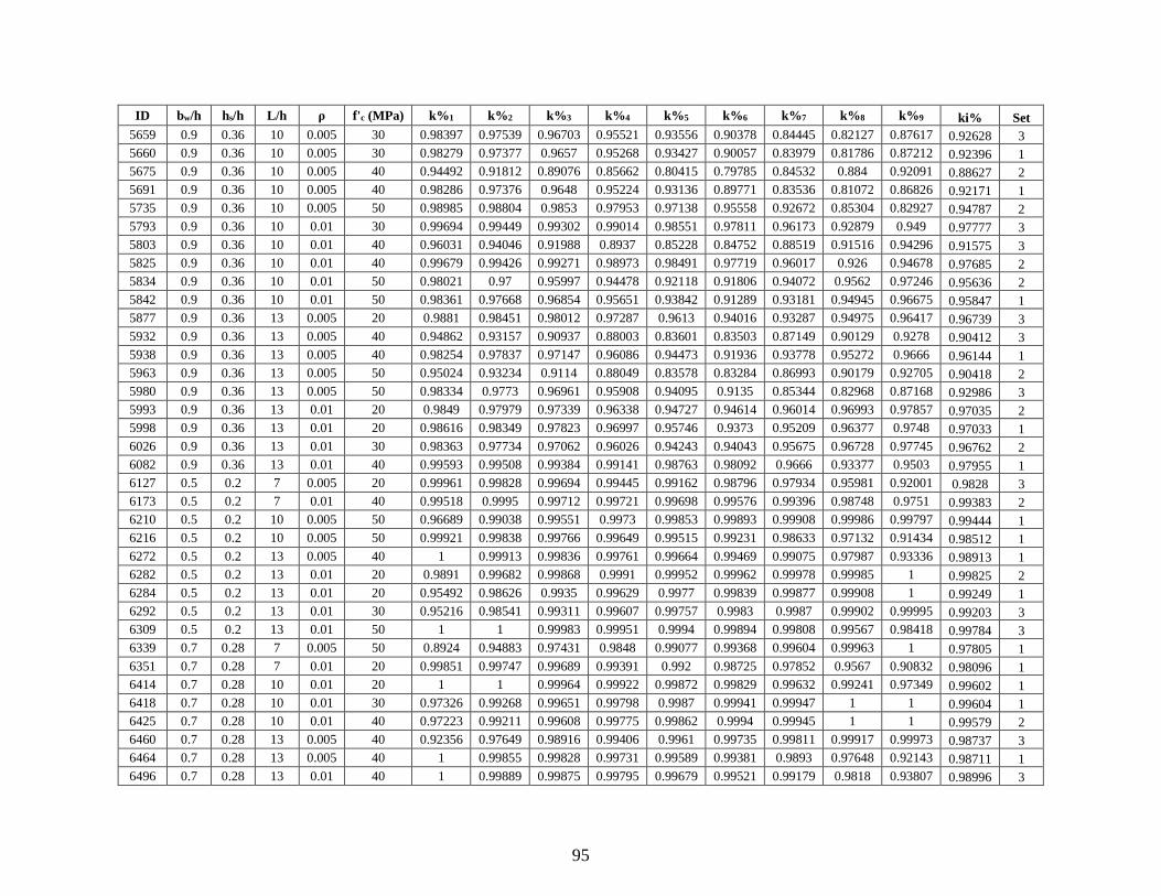
95

ID bw/h hs/h L/h ρ f'c (MPa) k%1 k%2 k%3 k%4 k%5 k%6 k%7 k%8 k%9 ki% Set

5659 0.9 0.36 10 0.005 30 0.98397 0.97539 0.96703 0.95521 0.93556 0.90378 0.84445 0.82127 0.87617 0.92628 3

5660 0.9 0.36 10 0.005 30 0.98279 0.97377 0.9657 0.95268 0.93427 0.90057 0.83979 0.81786 0.87212 0.92396 1

5675 0.9 0.36 10 0.005 40 0.94492 0.91812 0.89076 0.85662 0.80415 0.79785 0.84532 0.884 0.92091 0.88627 2

5691 0.9 0.36 10 0.005 40 0.98286 0.97376 0.9648 0.95224 0.93136 0.89771 0.83536 0.81072 0.86826 0.92171 1

5735 0.9 0.36 10 0.005 50 0.98985 0.98804 0.9853 0.97953 0.97138 0.95558 0.92672 0.85304 0.82927 0.94787 2

5793 0.9 0.36 10 0.01 30 0.99694 0.99449 0.99302 0.99014 0.98551 0.97811 0.96173 0.92879 0.949 0.97777 3

5803 0.9 0.36 10 0.01 40 0.96031 0.94046 0.91988 0.8937 0.85228 0.84752 0.88519 0.91516 0.94296 0.91575 3

5825 0.9 0.36 10 0.01 40 0.99679 0.99426 0.99271 0.98973 0.98491 0.97719 0.96017 0.926 0.94678 0.97685 2

5834 0.9 0.36 10 0.01 50 0.98021 0.97 0.95997 0.94478 0.92118 0.91806 0.94072 0.9562 0.97246 0.95636 2

5842 0.9 0.36 10 0.01 50 0.98361 0.97668 0.96854 0.95651 0.93842 0.91289 0.93181 0.94945 0.96675 0.95847 1

5877 0.9 0.36 13 0.005 20 0.9881 0.98451 0.98012 0.97287 0.9613 0.94016 0.93287 0.94975 0.96417 0.96739 3

5932 0.9 0.36 13 0.005 40 0.94862 0.93157 0.90937 0.88003 0.83601 0.83503 0.87149 0.90129 0.9278 0.90412 3

5938 0.9 0.36 13 0.005 40 0.98254 0.97837 0.97147 0.96086 0.94473 0.91936 0.93778 0.95272 0.9666 0.96144 1

5963 0.9 0.36 13 0.005 50 0.95024 0.93234 0.9114 0.88049 0.83578 0.83284 0.86993 0.90179 0.92705 0.90418 2

5980 0.9 0.36 13 0.005 50 0.98334 0.9773 0.96961 0.95908 0.94095 0.9135 0.85344 0.82968 0.87168 0.92986 3

5993 0.9 0.36 13 0.01 20 0.9849 0.97979 0.97339 0.96338 0.94727 0.94614 0.96014 0.96993 0.97857 0.97035 2

5998 0.9 0.36 13 0.01 20 0.98616 0.98349 0.97823 0.96997 0.95746 0.9373 0.95209 0.96377 0.9748 0.97033 1

6026 0.9 0.36 13 0.01 30 0.98363 0.97734 0.97062 0.96026 0.94243 0.94043 0.95675 0.96728 0.97745 0.96762 2

6082 0.9 0.36 13 0.01 40 0.99593 0.99508 0.99384 0.99141 0.98763 0.98092 0.9666 0.93377 0.9503 0.97955 1

6127 0.5 0.2 7 0.005 20 0.99961 0.99828 0.99694 0.99445 0.99162 0.98796 0.97934 0.95981 0.92001 0.9828 3

6173 0.5 0.2 7 0.01 40 0.99518 0.9995 0.99712 0.99721 0.99698 0.99576 0.99396 0.98748 0.9751 0.99383 2

6210 0.5 0.2 10 0.005 50 0.96689 0.99038 0.99551 0.9973 0.99853 0.99893 0.99908 0.99986 0.99797 0.99444 1

6216 0.5 0.2 10 0.005 50 0.99921 0.99838 0.99766 0.99649 0.99515 0.99231 0.98633 0.97132 0.91434 0.98512 1

6272 0.5 0.2 13 0.005 40 1 0.99913 0.99836 0.99761 0.99664 0.99469 0.99075 0.97987 0.93336 0.98913 1

6282 0.5 0.2 13 0.01 20 0.9891 0.99682 0.99868 0.9991 0.99952 0.99962 0.99978 0.99985 1 0.99825 2

6284 0.5 0.2 13 0.01 20 0.95492 0.98626 0.9935 0.99629 0.9977 0.99839 0.99877 0.99908 1 0.99249 1

6292 0.5 0.2 13 0.01 30 0.95216 0.98541 0.99311 0.99607 0.99757 0.9983 0.9987 0.99902 0.99995 0.99203 3

6309 0.5 0.2 13 0.01 50 1 1 0.99983 0.99951 0.9994 0.99894 0.99808 0.99567 0.98418 0.99784 3

6339 0.7 0.28 7 0.005 50 0.8924 0.94883 0.97431 0.9848 0.99077 0.99368 0.99604 0.99963 1 0.97805 1

6351 0.7 0.28 7 0.01 20 0.99851 0.99747 0.99689 0.99391 0.992 0.98725 0.97852 0.9567 0.90832 0.98096 1

6414 0.7 0.28 10 0.01 20 1 1 0.99964 0.99922 0.99872 0.99829 0.99632 0.99241 0.97349 0.99602 1

6418 0.7 0.28 10 0.01 30 0.97326 0.99268 0.99651 0.99798 0.9987 0.99941 0.99947 1 1 0.99604 1

6425 0.7 0.28 10 0.01 40 0.97223 0.99211 0.99608 0.99775 0.99862 0.9994 0.99945 1 1 0.99579 2

6460 0.7 0.28 13 0.005 40 0.92356 0.97649 0.98916 0.99406 0.9961 0.99735 0.99811 0.99917 0.99973 0.98737 3

6464 0.7 0.28 13 0.005 40 1 0.99855 0.99828 0.99731 0.99589 0.99381 0.9893 0.97648 0.92143 0.98711 1

6496 0.7 0.28 13 0.01 40 1 0.99889 0.99875 0.99795 0.99679 0.99521 0.99179 0.9818 0.93807 0.98996 3

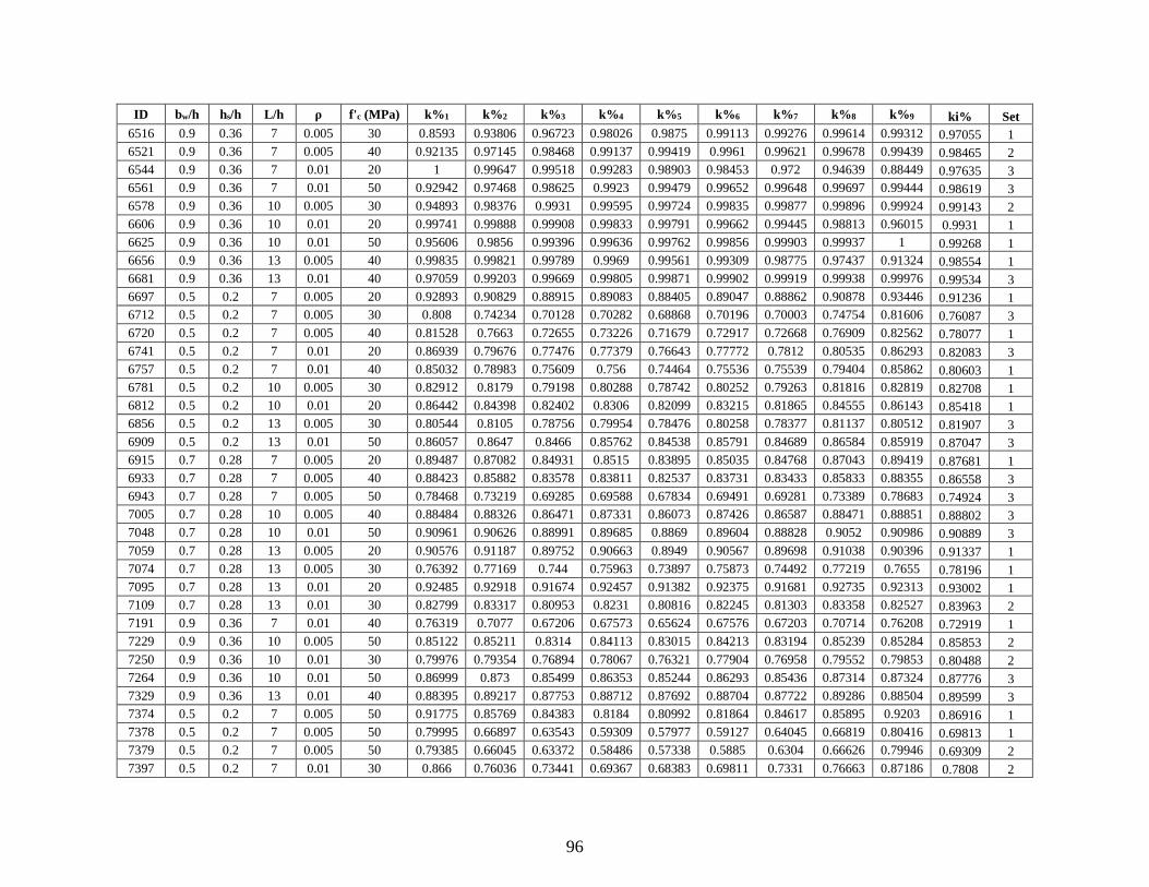
96

ID bw/h hs/h L/h ρ f'c (MPa) k%1 k%2 k%3 k%4 k%5 k%6 k%7 k%8 k%9 ki% Set

6516 0.9 0.36 7 0.005 30 0.8593 0.93806 0.96723 0.98026 0.9875 0.99113 0.99276 0.99614 0.99312 0.97055 1

6521 0.9 0.36 7 0.005 40 0.92135 0.97145 0.98468 0.99137 0.99419 0.9961 0.99621 0.99678 0.99439 0.98465 2

6544 0.9 0.36 7 0.01 20 1 0.99647 0.99518 0.99283 0.98903 0.98453 0.972 0.94639 0.88449 0.97635 3

6561 0.9 0.36 7 0.01 50 0.92942 0.97468 0.98625 0.9923 0.99479 0.99652 0.99648 0.99697 0.99444 0.98619 3

6578 0.9 0.36 10 0.005 30 0.94893 0.98376 0.9931 0.99595 0.99724 0.99835 0.99877 0.99896 0.99924 0.99143 2

6606 0.9 0.36 10 0.01 20 0.99741 0.99888 0.99908 0.99833 0.99791 0.99662 0.99445 0.98813 0.96015 0.9931 1

6625 0.9 0.36 10 0.01 50 0.95606 0.9856 0.99396 0.99636 0.99762 0.99856 0.99903 0.99937 1 0.99268 1

6656 0.9 0.36 13 0.005 40 0.99835 0.99821 0.99789 0.9969 0.99561 0.99309 0.98775 0.97437 0.91324 0.98554 1

6681 0.9 0.36 13 0.01 40 0.97059 0.99203 0.99669 0.99805 0.99871 0.99902 0.99919 0.99938 0.99976 0.99534 3

6697 0.5 0.2 7 0.005 20 0.92893 0.90829 0.88915 0.89083 0.88405 0.89047 0.88862 0.90878 0.93446 0.91236 1

6712 0.5 0.2 7 0.005 30 0.808 0.74234 0.70128 0.70282 0.68868 0.70196 0.70003 0.74754 0.81606 0.76087 3

6720 0.5 0.2 7 0.005 40 0.81528 0.7663 0.72655 0.73226 0.71679 0.72917 0.72668 0.76909 0.82562 0.78077 1

6741 0.5 0.2 7 0.01 20 0.86939 0.79676 0.77476 0.77379 0.76643 0.77772 0.7812 0.80535 0.86293 0.82083 3

6757 0.5 0.2 7 0.01 40 0.85032 0.78983 0.75609 0.756 0.74464 0.75536 0.75539 0.79404 0.85862 0.80603 1

6781 0.5 0.2 10 0.005 30 0.82912 0.8179 0.79198 0.80288 0.78742 0.80252 0.79263 0.81816 0.82819 0.82708 1

6812 0.5 0.2 10 0.01 20 0.86442 0.84398 0.82402 0.8306 0.82099 0.83215 0.81865 0.84555 0.86143 0.85418 1

6856 0.5 0.2 13 0.005 30 0.80544 0.8105 0.78756 0.79954 0.78476 0.80258 0.78377 0.81137 0.80512 0.81907 3

6909 0.5 0.2 13 0.01 50 0.86057 0.8647 0.8466 0.85762 0.84538 0.85791 0.84689 0.86584 0.85919 0.87047 3

6915 0.7 0.28 7 0.005 20 0.89487 0.87082 0.84931 0.8515 0.83895 0.85035 0.84768 0.87043 0.89419 0.87681 1

6933 0.7 0.28 7 0.005 40 0.88423 0.85882 0.83578 0.83811 0.82537 0.83731 0.83433 0.85833 0.88355 0.86558 3

6943 0.7 0.28 7 0.005 50 0.78468 0.73219 0.69285 0.69588 0.67834 0.69491 0.69281 0.73389 0.78683 0.74924 3

7005 0.7 0.28 10 0.005 40 0.88484 0.88326 0.86471 0.87331 0.86073 0.87426 0.86587 0.88471 0.88851 0.88802 3

7048 0.7 0.28 10 0.01 50 0.90961 0.90626 0.88991 0.89685 0.8869 0.89604 0.88828 0.9052 0.90986 0.90889 3

7059 0.7 0.28 13 0.005 20 0.90576 0.91187 0.89752 0.90663 0.8949 0.90567 0.89698 0.91038 0.90396 0.91337 1

7074 0.7 0.28 13 0.005 30 0.76392 0.77169 0.744 0.75963 0.73897 0.75873 0.74492 0.77219 0.7655 0.78196 1

7095 0.7 0.28 13 0.01 20 0.92485 0.92918 0.91674 0.92457 0.91382 0.92375 0.91681 0.92735 0.92313 0.93002 1

7109 0.7 0.28 13 0.01 30 0.82799 0.83317 0.80953 0.8231 0.80816 0.82245 0.81303 0.83358 0.82527 0.83963 2

7191 0.9 0.36 7 0.01 40 0.76319 0.7077 0.67206 0.67573 0.65624 0.67576 0.67203 0.70714 0.76208 0.72919 1

7229 0.9 0.36 10 0.005 50 0.85122 0.85211 0.8314 0.84113 0.83015 0.84213 0.83194 0.85239 0.85284 0.85853 2

7250 0.9 0.36 10 0.01 30 0.79976 0.79354 0.76894 0.78067 0.76321 0.77904 0.76958 0.79552 0.79853 0.80488 2

7264 0.9 0.36 10 0.01 50 0.86999 0.873 0.85499 0.86353 0.85244 0.86293 0.85436 0.87314 0.87324 0.87776 3

7329 0.9 0.36 13 0.01 40 0.88395 0.89217 0.87753 0.88712 0.87692 0.88704 0.87722 0.89286 0.88504 0.89599 3

7374 0.5 0.2 7 0.005 50 0.91775 0.85769 0.84383 0.8184 0.80992 0.81864 0.84617 0.85895 0.9203 0.86916 1

7378 0.5 0.2 7 0.005 50 0.79995 0.66897 0.63543 0.59309 0.57977 0.59127 0.64045 0.66819 0.80416 0.69813 1

7379 0.5 0.2 7 0.005 50 0.79385 0.66045 0.63372 0.58486 0.57338 0.5885 0.6304 0.66626 0.79946 0.69309 2

7397 0.5 0.2 7 0.01 30 0.866 0.76036 0.73441 0.69367 0.68383 0.69811 0.7331 0.76663 0.87186 0.7808 2

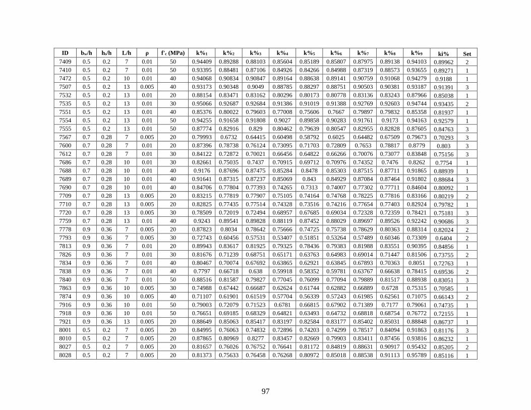
97

ID bw/h hs/h L/h ρ f'c (MPa) k%1 k%2 k%3 k%4 k%5 k%6 k%7 k%8 k%9 ki% Set

7409 0.5 0.2 7 0.01 50 0.94409 0.89288 0.88103 0.85604 0.85189 0.85807 0.87975 0.89138 0.94103 0.89962 2

7410 0.5 0.2 7 0.01 50 0.93395 0.88481 0.87106 0.84926 0.84266 0.84988 0.87319 0.88573 0.93655 0.89271 1

7472 0.5 0.2 10 0.01 40 0.94068 0.90834 0.90847 0.89164 0.88638 0.89141 0.90759 0.91068 0.94279 0.9188 1

7507 0.5 0.2 13 0.005 40 0.93173 0.90348 0.9049 0.88785 0.88297 0.88751 0.90503 0.90381 0.93187 0.91391 3

7532 0.5 0.2 13 0.01 20 0.88154 0.83471 0.83162 0.80296 0.80173 0.80778 0.83136 0.83243 0.87966 0.85038 1

7535 0.5 0.2 13 0.01 30 0.95066 0.92687 0.92684 0.91386 0.91019 0.91388 0.92769 0.92603 0.94744 0.93435 2

7551 0.5 0.2 13 0.01 40 0.85376 0.80022 0.79603 0.77008 0.75606 0.7667 0.79897 0.79832 0.85358 0.81937 1

7554 0.5 0.2 13 0.01 50 0.94255 0.91658 0.91808 0.9027 0.89858 0.90283 0.91761 0.9173 0.94163 0.92579 1

7555 0.5 0.2 13 0.01 50 0.87774 0.82916 0.829 0.80462 0.79639 0.80547 0.82955 0.82828 0.87605 0.84763 3

7567 0.7 0.28 7 0.005 20 0.79993 0.6732 0.64415 0.60498 0.58792 0.6025 0.64482 0.67509 0.79673 0.70293 3

7600 0.7 0.28 7 0.01 20 0.87396 0.78738 0.76124 0.73095 0.71703 0.72809 0.7653 0.78817 0.8779 0.803 3

7612 0.7 0.28 7 0.01 30 0.84122 0.72872 0.70021 0.66456 0.64822 0.66266 0.70076 0.73077 0.83848 0.75156 3

7686 0.7 0.28 10 0.01 30 0.82661 0.75035 0.7437 0.70915 0.69712 0.70976 0.74352 0.7476 0.8262 0.7754 1

7688 0.7 0.28 10 0.01 40 0.9176 0.87696 0.87475 0.85284 0.8478 0.85303 0.87515 0.87711 0.91865 0.88939 1

7689 0.7 0.28 10 0.01 40 0.91641 0.87315 0.87237 0.85069 0.843 0.84929 0.87084 0.87464 0.91802 0.88684 3

7690 0.7 0.28 10 0.01 40 0.84706 0.77804 0.77393 0.74265 0.7313 0.74007 0.77302 0.77711 0.84604 0.80092 1

7709 0.7 0.28 13 0.005 20 0.83215 0.77819 0.77907 0.75105 0.74164 0.74768 0.78225 0.77816 0.83166 0.80219 2

7710 0.7 0.28 13 0.005 20 0.82825 0.77435 0.77514 0.74328 0.73516 0.74216 0.77654 0.77403 0.82924 0.79782 1

7720 0.7 0.28 13 0.005 30 0.78509 0.72019 0.72494 0.68957 0.67685 0.69034 0.72328 0.72359 0.78421 0.75181 3

7759 0.7 0.28 13 0.01 40 0.9243 0.89541 0.89828 0.88119 0.87452 0.88029 0.89697 0.89526 0.92242 0.90686 3

7778 0.9 0.36 7 0.005 20 0.87823 0.8034 0.78642 0.75666 0.74725 0.75738 0.78629 0.80363 0.88314 0.82024 2

7793 0.9 0.36 7 0.005 30 0.72743 0.60456 0.57531 0.53407 0.51851 0.53264 0.57489 0.60346 0.73309 0.6404 2

7813 0.9 0.36 7 0.01 20 0.89943 0.83617 0.81925 0.79325 0.78436 0.79383 0.81988 0.83551 0.90395 0.84856 1

7826 0.9 0.36 7 0.01 30 0.81676 0.71239 0.68751 0.65171 0.63763 0.64983 0.69014 0.71447 0.81506 0.73755 2

7834 0.9 0.36 7 0.01 40 0.80467 0.70074 0.67692 0.63865 0.62921 0.63845 0.67893 0.70363 0.8051 0.72763 1

7838 0.9 0.36 7 0.01 40 0.7797 0.66718 0.638 0.59918 0.58352 0.59781 0.63767 0.66638 0.78415 0.69536 2

7840 0.9 0.36 7 0.01 50 0.88516 0.81587 0.79827 0.77045 0.76099 0.77094 0.79889 0.81517 0.88938 0.83051 3

7863 0.9 0.36 10 0.005 30 0.74988 0.67442 0.66687 0.62624 0.61744 0.62882 0.66889 0.6728 0.75315 0.70585 1

7874 0.9 0.36 10 0.005 40 0.71107 0.61901 0.61519 0.57704 0.56339 0.57243 0.61985 0.62561 0.71075 0.66143 2

7916 0.9 0.36 10 0.01 50 0.79003 0.72079 0.71523 0.6781 0.66815 0.67902 0.71389 0.7177 0.79061 0.74735 1

7918 0.9 0.36 10 0.01 50 0.76651 0.69185 0.68329 0.64821 0.63493 0.64732 0.68818 0.68754 0.76772 0.72155 1

7921 0.9 0.36 13 0.005 20 0.88649 0.85063 0.85417 0.83197 0.82584 0.83177 0.85402 0.85031 0.88848 0.86737 1

8001 0.5 0.2 7 0.005 20 0.84995 0.76063 0.74832 0.72896 0.74203 0.74299 0.78517 0.84094 0.91863 0.81176 3

8010 0.5 0.2 7 0.005 20 0.87865 0.80969 0.8277 0.83457 0.82669 0.79903 0.83411 0.87456 0.93816 0.86232 1

8027 0.5 0.2 7 0.005 20 0.81657 0.76026 0.76752 0.76641 0.81172 0.84819 0.88631 0.90917 0.95432 0.85205 2

8028 0.5 0.2 7 0.005 20 0.81373 0.75633 0.76458 0.76268 0.80972 0.85018 0.88538 0.91113 0.95789 0.85116 1

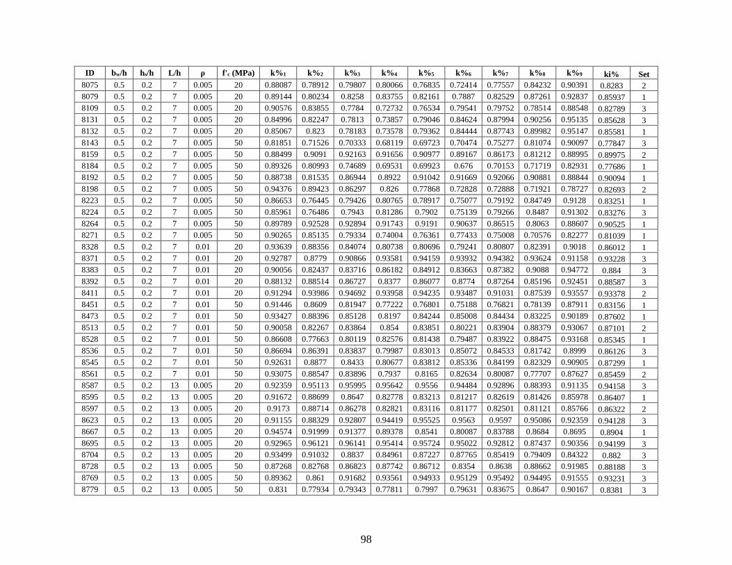
98

ID bw/h hs/h L/h ρ f'c (MPa) k%1 k%2 k%3 k%4 k%5 k%6 k%7 k%8 k%9 ki% Set

8075 0.5 0.2 7 0.005 20 0.88087 0.78912 0.79807 0.80066 0.76835 0.72414 0.77557 0.84232 0.90391 0.8283 2

8079 0.5 0.2 7 0.005 20 0.89144 0.80234 0.8258 0.83755 0.82161 0.7887 0.82529 0.87261 0.92837 0.85937 1

8109 0.5 0.2 7 0.005 20 0.90576 0.83855 0.7784 0.72732 0.76534 0.79541 0.79752 0.78514 0.88548 0.82789 3

8131 0.5 0.2 7 0.005 20 0.84996 0.82247 0.7813 0.73857 0.79046 0.84624 0.87994 0.90256 0.95135 0.85628 3

8132 0.5 0.2 7 0.005 20 0.85067 0.823 0.78183 0.73578 0.79362 0.84444 0.87743 0.89982 0.95147 0.85581 1

8143 0.5 0.2 7 0.005 50 0.81851 0.71526 0.70333 0.68119 0.69723 0.70474 0.75277 0.81074 0.90097 0.77847 3

8159 0.5 0.2 7 0.005 50 0.88499 0.9091 0.92163 0.91656 0.90977 0.89167 0.86173 0.81212 0.88995 0.89975 2

8184 0.5 0.2 7 0.005 50 0.89326 0.80993 0.74689 0.69531 0.69923 0.676 0.70153 0.71719 0.82931 0.77686 1

8192 0.5 0.2 7 0.005 50 0.88738 0.81535 0.86944 0.8922 0.91042 0.91669 0.92066 0.90881 0.88844 0.90094 1

8198 0.5 0.2 7 0.005 50 0.94376 0.89423 0.86297 0.826 0.77868 0.72828 0.72888 0.71921 0.78727 0.82693 2

8223 0.5 0.2 7 0.005 50 0.86653 0.76445 0.79426 0.80765 0.78917 0.75077 0.79192 0.84749 0.9128 0.83251 1

8224 0.5 0.2 7 0.005 50 0.85961 0.76486 0.7943 0.81286 0.7902 0.75139 0.79266 0.8487 0.91302 0.83276 3

8264 0.5 0.2 7 0.005 50 0.89789 0.92528 0.92894 0.91743 0.9191 0.90637 0.86515 0.8063 0.88607 0.90525 1

8271 0.5 0.2 7 0.005 50 0.90265 0.85135 0.79334 0.74004 0.76361 0.77433 0.75008 0.70576 0.82277 0.81039 1

8328 0.5 0.2 7 0.01 20 0.93639 0.88356 0.84074 0.80738 0.80696 0.79241 0.80807 0.82391 0.9018 0.86012 1

8371 0.5 0.2 7 0.01 20 0.92787 0.8779 0.90866 0.93581 0.94159 0.93932 0.94382 0.93624 0.91158 0.93228 3

8383 0.5 0.2 7 0.01 20 0.90056 0.82437 0.83716 0.86182 0.84912 0.83663 0.87382 0.9088 0.94772 0.884 3

8392 0.5 0.2 7 0.01 20 0.88132 0.88514 0.86727 0.8377 0.86077 0.8774 0.87264 0.85196 0.92451 0.88587 3

8411 0.5 0.2 7 0.01 20 0.91294 0.93986 0.94692 0.93958 0.94235 0.93487 0.91031 0.87539 0.93557 0.93378 2

8451 0.5 0.2 7 0.01 50 0.91446 0.8609 0.81947 0.77222 0.76801 0.75188 0.76821 0.78139 0.87911 0.83156 1

8473 0.5 0.2 7 0.01 50 0.93427 0.88396 0.85128 0.8197 0.84244 0.85008 0.84434 0.83225 0.90189 0.87602 1

8513 0.5 0.2 7 0.01 50 0.90058 0.82267 0.83864 0.854 0.83851 0.80221 0.83904 0.88379 0.93067 0.87101 2

8528 0.5 0.2 7 0.01 50 0.86608 0.77663 0.80119 0.82576 0.81438 0.79487 0.83922 0.88475 0.93168 0.85345 1

8536 0.5 0.2 7 0.01 50 0.86694 0.86391 0.83837 0.79987 0.83013 0.85072 0.84533 0.81742 0.8999 0.86126 3

8545 0.5 0.2 7 0.01 50 0.92631 0.8877 0.8433 0.80677 0.83812 0.85336 0.84199 0.82329 0.90905 0.87299 1

8561 0.5 0.2 7 0.01 50 0.93075 0.88547 0.83896 0.7937 0.8165 0.82634 0.80087 0.77707 0.87627 0.85459 2

8587 0.5 0.2 13 0.005 20 0.92359 0.95113 0.95995 0.95642 0.9556 0.94484 0.92896 0.88393 0.91135 0.94158 3

8595 0.5 0.2 13 0.005 20 0.91672 0.88699 0.8647 0.82778 0.83213 0.81217 0.82619 0.81426 0.85978 0.86407 1

8597 0.5 0.2 13 0.005 20 0.9173 0.88714 0.86278 0.82821 0.83116 0.81177 0.82501 0.81121 0.85766 0.86322 2

8623 0.5 0.2 13 0.005 20 0.91155 0.88329 0.92807 0.94419 0.95525 0.9563 0.9597 0.95086 0.92359 0.94128 3

8667 0.5 0.2 13 0.005 20 0.94574 0.91999 0.91377 0.89378 0.8541 0.80087 0.83788 0.8684 0.8695 0.8904 1

8695 0.5 0.2 13 0.005 20 0.92965 0.96121 0.96141 0.95414 0.95724 0.95022 0.92812 0.87437 0.90356 0.94199 3

8704 0.5 0.2 13 0.005 20 0.93499 0.91032 0.8837 0.84961 0.87227 0.87765 0.85419 0.79409 0.84322 0.882 3

8728 0.5 0.2 13 0.005 50 0.87268 0.82768 0.86823 0.87742 0.86712 0.8354 0.8638 0.88662 0.91985 0.88188 3

8769 0.5 0.2 13 0.005 50 0.89362 0.861 0.91682 0.93561 0.94933 0.95129 0.95492 0.94495 0.91555 0.93231 3

8779 0.5 0.2 13 0.005 50 0.831 0.77934 0.79343 0.77811 0.7997 0.79631 0.83675 0.8647 0.90167 0.8381 3

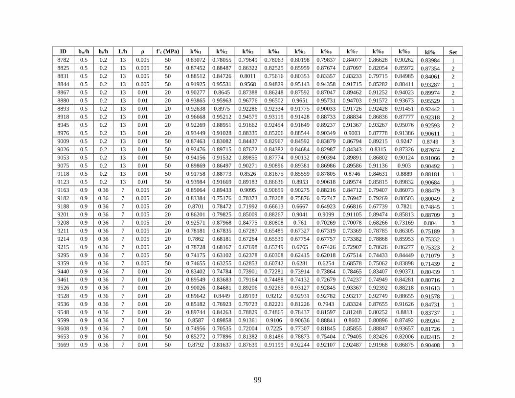
99

ID bw/h hs/h L/h ρ f'c (MPa) k%1 k%2 k%3 k%4 k%5 k%6 k%7 k%8 k%9 ki% Set

8782 0.5 0.2 13 0.005 50 0.83072 0.78055 0.79649 0.78063 0.80198 0.79837 0.84077 0.86628 0.90262 0.83984 1

8825 0.5 0.2 13 0.005 50 0.87452 0.88487 0.86322 0.82525 0.85959 0.87674 0.87097 0.82054 0.85972 0.87354 2

8831 0.5 0.2 13 0.005 50 0.88512 0.84726 0.8011 0.75616 0.80353 0.83357 0.83233 0.79715 0.84985 0.84061 2

8844 0.5 0.2 13 0.005 50 0.91925 0.95531 0.9568 0.94829 0.95143 0.94358 0.91715 0.85282 0.88411 0.93287 1

8867 0.5 0.2 13 0.01 20 0.90277 0.8645 0.87388 0.86248 0.87592 0.87047 0.89462 0.91252 0.94023 0.89974 2

8880 0.5 0.2 13 0.01 20 0.93865 0.95963 0.96776 0.96502 0.9651 0.95731 0.94703 0.91572 0.93673 0.95529 1

8893 0.5 0.2 13 0.01 20 0.92638 0.8975 0.92286 0.92334 0.91775 0.90033 0.91726 0.92428 0.91451 0.92442 1

8918 0.5 0.2 13 0.01 20 0.96668 0.95212 0.94575 0.93119 0.91428 0.88733 0.88834 0.86836 0.87777 0.92318 2

8945 0.5 0.2 13 0.01 20 0.92269 0.88951 0.91662 0.92454 0.91649 0.89237 0.91367 0.93267 0.95076 0.92593 2

8976 0.5 0.2 13 0.01 20 0.93449 0.91028 0.88335 0.85206 0.88544 0.90349 0.9003 0.87778 0.91386 0.90611 1

9009 0.5 0.2 13 0.01 50 0.87463 0.83082 0.84437 0.82967 0.84592 0.83879 0.86794 0.89215 0.9247 0.8749 3

9026 0.5 0.2 13 0.01 50 0.92476 0.89715 0.87672 0.84382 0.84684 0.82987 0.84343 0.8315 0.87326 0.87674 2

9053 0.5 0.2 13 0.01 50 0.94156 0.91532 0.89855 0.87774 0.90132 0.90394 0.89891 0.86802 0.90124 0.91066 2

9075 0.5 0.2 13 0.01 50 0.89869 0.86497 0.90271 0.90896 0.89381 0.86986 0.89586 0.91136 0.903 0.90492 1

9118 0.5 0.2 13 0.01 50 0.91758 0.88773 0.8526 0.81675 0.85559 0.87805 0.8746 0.84631 0.8889 0.88181 1

9123 0.5 0.2 13 0.01 50 0.93984 0.91669 0.89183 0.86636 0.8953 0.90618 0.89574 0.85815 0.89832 0.90684 1

9163 0.9 0.36 7 0.005 20 0.85064 0.89433 0.9095 0.90659 0.90275 0.88216 0.84712 0.79407 0.86073 0.88479 3

9182 0.9 0.36 7 0.005 20 0.83384 0.75176 0.78373 0.78208 0.75876 0.72747 0.76947 0.79269 0.80503 0.80049 2

9188 0.9 0.36 7 0.005 20 0.8701 0.78472 0.71992 0.66613 0.6667 0.64923 0.66816 0.67739 0.7821 0.74845 1

9201 0.9 0.36 7 0.005 20 0.86201 0.79825 0.85009 0.88267 0.9041 0.9099 0.91105 0.89474 0.85813 0.88709 3

9208 0.9 0.36 7 0.005 20 0.92571 0.87968 0.84775 0.80808 0.761 0.70269 0.70078 0.68266 0.73169 0.804 3

9211 0.9 0.36 7 0.005 20 0.78181 0.67835 0.67287 0.65485 0.67327 0.67319 0.73369 0.78785 0.86305 0.75189 3

9214 0.9 0.36 7 0.005 20 0.7862 0.68181 0.67264 0.65539 0.67754 0.67757 0.73382 0.78868 0.85953 0.75332 1

9215 0.9 0.36 7 0.005 20 0.78728 0.68167 0.67698 0.65749 0.6765 0.67426 0.72907 0.78626 0.86277 0.75323 2

9295 0.9 0.36 7 0.005 50 0.74175 0.63102 0.62378 0.60308 0.62415 0.62018 0.67514 0.74433 0.84449 0.71079 3

9359 0.9 0.36 7 0.005 50 0.74655 0.63255 0.62853 0.60742 0.6281 0.6254 0.68578 0.75062 0.83898 0.71439 2

9440 0.9 0.36 7 0.01 20 0.83402 0.74784 0.73901 0.72281 0.73914 0.73864 0.78465 0.83407 0.90371 0.80439 1

9461 0.9 0.36 7 0.01 20 0.89549 0.83683 0.79164 0.74488 0.74132 0.72679 0.74237 0.74949 0.84281 0.80716 2

9526 0.9 0.36 7 0.01 20 0.90026 0.84681 0.89206 0.92265 0.93127 0.92845 0.93367 0.92392 0.88218 0.91613 1

9528 0.9 0.36 7 0.01 20 0.89642 0.8449 0.89193 0.9212 0.92931 0.92782 0.93217 0.92749 0.88655 0.91578 1

9536 0.9 0.36 7 0.01 20 0.85182 0.76923 0.79723 0.82221 0.81226 0.7943 0.83324 0.87655 0.91626 0.84731 1

9548 0.9 0.36 7 0.01 20 0.89744 0.84263 0.78829 0.74865 0.78437 0.81597 0.81248 0.80252 0.8813 0.83737 1

9599 0.9 0.36 7 0.01 50 0.8587 0.89858 0.91361 0.9106 0.90636 0.88841 0.8602 0.80896 0.87492 0.89204 2

9608 0.9 0.36 7 0.01 50 0.74956 0.70535 0.72004 0.7225 0.77307 0.81845 0.85855 0.88847 0.93657 0.81726 1

9653 0.9 0.36 7 0.01 50 0.85272 0.77896 0.81382 0.81486 0.78873 0.75404 0.79405 0.82426 0.82006 0.82415 2

9669 0.9 0.36 7 0.01 50 0.8792 0.81637 0.87639 0.91199 0.92244 0.92107 0.92487 0.91968 0.86875 0.90408 3

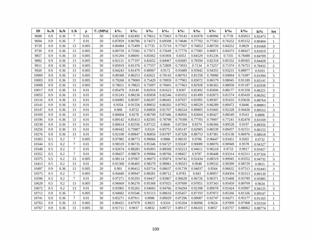
100

ID bw/h hs/h L/h ρ f'c (MPa) k%1 k%2 k%3 k%4 k%5 k%6 k%7 k%8 k%9 ki% Set

9688 0.9 0.36 7 0.01 50 0.82198 0.82492 0.79612 0.75963 0.79143 0.81878 0.80996 0.7739 0.85053 0.82473 3

9694 0.9 0.36 7 0.01 50 0.87859 0.80786 0.74571 0.69508 0.74646 0.77702 0.77563 0.76252 0.85152 0.80404 1

9729 0.9 0.36 13 0.005 20 0.80484 0.75499 0.7735 0.75716 0.77507 0.76853 0.80726 0.84252 0.8829 0.81668 3

9730 0.9 0.36 13 0.005 20 0.80759 0.75582 0.77671 0.75649 0.77776 0.77085 0.80871 0.84373 0.88427 0.81819 1

9857 0.9 0.36 13 0.005 20 0.91204 0.88691 0.85062 0.81004 0.8353 0.84529 0.81236 0.7335 0.78488 0.84709 2

9882 0.9 0.36 13 0.005 50 0.82131 0.77197 0.82652 0.84067 0.82685 0.78594 0.82318 0.85332 0.89305 0.84428 1

9911 0.9 0.36 13 0.005 50 0.85919 0.81376 0.77557 0.72809 0.73933 0.7134 0.73257 0.71374 0.76753 0.78432 2

9920 0.9 0.36 13 0.005 50 0.84243 0.81479 0.88967 0.9172 0.93489 0.93942 0.94355 0.93231 0.88877 0.9103 1

10000 0.9 0.36 13 0.005 50 0.89368 0.86253 0.82621 0.78143 0.80763 0.81258 0.78086 0.69064 0.74387 0.81994 3

10003 0.9 0.36 13 0.005 50 0.79268 0.79069 0.75429 0.70859 0.77902 0.83072 0.86579 0.88045 0.91189 0.83141 3

10008 0.9 0.36 13 0.005 50 0.78651 0.78825 0.75097 0.70605 0.77663 0.82928 0.86365 0.88058 0.91187 0.82938 1

10017 0.9 0.36 13 0.01 20 0.85479 0.8149 0.82916 0.81623 0.8307 0.82492 0.85606 0.88177 0.91358 0.86221 3

10055 0.9 0.36 13 0.01 20 0.91243 0.88236 0.85858 0.82546 0.83352 0.81499 0.82873 0.81574 0.85439 0.86262 2

10116 0.9 0.36 13 0.01 20 0.84085 0.80397 0.86207 0.88445 0.87937 0.85995 0.89307 0.91633 0.93636 0.88764 1

10141 0.9 0.36 13 0.01 20 0.9354 0.91556 0.89032 0.86202 0.87952 0.88529 0.86289 0.80472 0.8446 0.88803 1

10147 0.9 0.36 13 0.01 20 0.868 0.8722 0.84856 0.81707 0.86524 0.89805 0.91845 0.92328 0.94436 0.89552 3

10169 0.9 0.36 13 0.01 50 0.86604 0.8278 0.86708 0.87446 0.86856 0.83604 0.86427 0.88549 0.9163 0.8806 2

10196 0.9 0.36 13 0.01 50 0.89142 0.85413 0.82505 0.78798 0.79398 0.77705 0.79007 0.77241 0.82478 0.83169 1

10238 0.9 0.36 13 0.01 50 0.86614 0.82556 0.87122 0.8846 0.87204 0.8374 0.86366 0.89528 0.9197 0.88356 2

10256 0.9 0.36 13 0.01 50 0.80442 0.75887 0.8324 0.85751 0.85147 0.82905 0.86539 0.89457 0.92151 0.86152 1

10276 0.9 0.36 13 0.01 50 0.92108 0.89847 0.86856 0.83787 0.87328 0.88753 0.87381 0.83138 0.86976 0.88618 3

10303 0.5 0.2 7 0.005 20 0.97985 0.98773 0.99066 0.9886 0.98535 0.9786 0.96647 0.93451 0.9202 0.9732 3

10344 0.5 0.2 7 0.01 20 0.98319 0.96735 0.95346 0.94727 0.93247 0.90089 0.88076 0.90949 0.9578 0.94327 1

10348 0.5 0.2 7 0.01 50 0.92674 0.88283 0.85003 0.88568 0.92213 0.94611 0.96218 0.9753 0.9917 0.93427 3

10352 0.5 0.2 7 0.01 50 0.98437 0.98878 0.99084 0.98766 0.98457 0.9787 0.96448 0.93314 0.92311 0.97356 1

10375 0.5 0.2 13 0.005 20 0.98114 0.97067 0.96073 0.95874 0.94742 0.92434 0.88519 0.90945 0.93552 0.94732 3

10413 0.5 0.2 13 0.01 50 0.91368 0.96405 0.98279 0.98981 0.99323 0.9948 0.99532 0.99399 0.98729 0.9815 3

10497 0.9 0.36 13 0.005 20 0.901 0.86412 0.83714 0.88637 0.91739 0.94037 0.9564 0.96632 0.97513 0.92443 3

10575 0.5 0.2 7 0.005 50 0.94449 0.90947 0.88281 0.88712 0.8783 0.843 0.80057 0.84504 0.92313 0.89139 1

10596 0.5 0.2 7 0.01 20 0.97271 0.95293 0.94437 0.95867 0.96628 0.96726 0.96371 0.93468 0.93789 0.95985 1

10628 0.5 0.2 13 0.005 20 0.96669 0.96276 0.95368 0.97025 0.97699 0.97851 0.97343 0.95459 0.89709 0.9634 1

10672 0.5 0.2 13 0.01 50 0.95965 0.95265 0.94065 0.94766 0.94294 0.92398 0.89078 0.91424 0.93997 0.94125 3

10712 0.9 0.36 7 0.005 50 0.94682 0.93546 0.91513 0.88616 0.85457 0.87193 0.87872 0.85266 0.81326 0.89547 1

10741 0.9 0.36 7 0.01 50 0.85271 0.87911 0.8986 0.89029 0.87296 0.90087 0.92747 0.94271 0.95177 0.91165 1

10765 0.9 0.36 13 0.005 50 0.80425 0.87979 0.8923 0.9316 0.95204 0.96096 0.9624 0.97099 0.97908 0.93334 1

10767 0.9 0.36 13 0.005 50 0.91711 0.9037 0.8832 0.89727 0.89117 0.86103 0.8057 0.83757 0.88062 0.88774 1

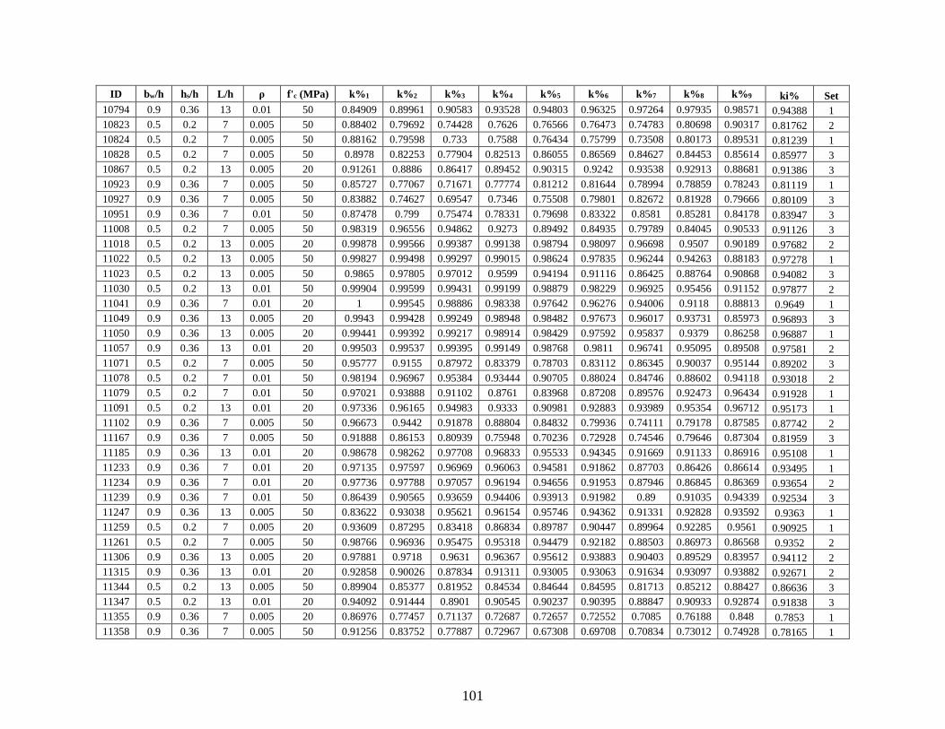
101

ID bw/h hs/h L/h ρ f'c (MPa) k%1 k%2 k%3 k%4 k%5 k%6 k%7 k%8 k%9 ki% Set

10794 0.9 0.36 13 0.01 50 0.84909 0.89961 0.90583 0.93528 0.94803 0.96325 0.97264 0.97935 0.98571 0.94388 1

10823 0.5 0.2 7 0.005 50 0.88402 0.79692 0.74428 0.7626 0.76566 0.76473 0.74783 0.80698 0.90317 0.81762 2

10824 0.5 0.2 7 0.005 50 0.88162 0.79598 0.733 0.7588 0.76434 0.75799 0.73508 0.80173 0.89531 0.81239 1

10828 0.5 0.2 7 0.005 50 0.8978 0.82253 0.77904 0.82513 0.86055 0.86569 0.84627 0.84453 0.85614 0.85977 3

10867 0.5 0.2 13 0.005 20 0.91261 0.8886 0.86417 0.89452 0.90315 0.9242 0.93538 0.92913 0.88681 0.91386 3

10923 0.9 0.36 7 0.005 50 0.85727 0.77067 0.71671 0.77774 0.81212 0.81644 0.78994 0.78859 0.78243 0.81119 1

10927 0.9 0.36 7 0.005 50 0.83882 0.74627 0.69547 0.7346 0.75508 0.79801 0.82672 0.81928 0.79666 0.80109 3

10951 0.9 0.36 7 0.01 50 0.87478 0.799 0.75474 0.78331 0.79698 0.83322 0.8581 0.85281 0.84178 0.83947 3

11008 0.5 0.2 7 0.005 50 0.98319 0.96556 0.94862 0.9273 0.89492 0.84935 0.79789 0.84045 0.90533 0.91126 3

11018 0.5 0.2 13 0.005 20 0.99878 0.99566 0.99387 0.99138 0.98794 0.98097 0.96698 0.9507 0.90189 0.97682 2

11022 0.5 0.2 13 0.005 50 0.99827 0.99498 0.99297 0.99015 0.98624 0.97835 0.96244 0.94263 0.88183 0.97278 1

11023 0.5 0.2 13 0.005 50 0.9865 0.97805 0.97012 0.9599 0.94194 0.91116 0.86425 0.88764 0.90868 0.94082 3

11030 0.5 0.2 13 0.01 50 0.99904 0.99599 0.99431 0.99199 0.98879 0.98229 0.96925 0.95456 0.91152 0.97877 2

11041 0.9 0.36 7 0.01 20 1 0.99545 0.98886 0.98338 0.97642 0.96276 0.94006 0.9118 0.88813 0.9649 1

11049 0.9 0.36 13 0.005 20 0.9943 0.99428 0.99249 0.98948 0.98482 0.97673 0.96017 0.93731 0.85973 0.96893 3

11050 0.9 0.36 13 0.005 20 0.99441 0.99392 0.99217 0.98914 0.98429 0.97592 0.95837 0.9379 0.86258 0.96887 1

11057 0.9 0.36 13 0.01 20 0.99503 0.99537 0.99395 0.99149 0.98768 0.9811 0.96741 0.95095 0.89508 0.97581 2

11071 0.5 0.2 7 0.005 50 0.95777 0.9155 0.87972 0.83379 0.78703 0.83112 0.86345 0.90037 0.95144 0.89202 3

11078 0.5 0.2 7 0.01 50 0.98194 0.96967 0.95384 0.93444 0.90705 0.88024 0.84746 0.88602 0.94118 0.93018 2

11079 0.5 0.2 7 0.01 50 0.97021 0.93888 0.91102 0.8761 0.83968 0.87208 0.89576 0.92473 0.96434 0.91928 1

11091 0.5 0.2 13 0.01 20 0.97336 0.96165 0.94983 0.9333 0.90981 0.92883 0.93989 0.95354 0.96712 0.95173 1

11102 0.9 0.36 7 0.005 50 0.96673 0.9442 0.91878 0.88804 0.84832 0.79936 0.74111 0.79178 0.87585 0.87742 2

11167 0.9 0.36 7 0.005 50 0.91888 0.86153 0.80939 0.75948 0.70236 0.72928 0.74546 0.79646 0.87304 0.81959 3

11185 0.9 0.36 13 0.01 20 0.98678 0.98262 0.97708 0.96833 0.95533 0.94345 0.91669 0.91133 0.86916 0.95108 1

11233 0.9 0.36 7 0.01 20 0.97135 0.97597 0.96969 0.96063 0.94581 0.91862 0.87703 0.86426 0.86614 0.93495 1

11234 0.9 0.36 7 0.01 20 0.97736 0.97788 0.97057 0.96194 0.94656 0.91953 0.87946 0.86845 0.86369 0.93654 2

11239 0.9 0.36 7 0.01 50 0.86439 0.90565 0.93659 0.94406 0.93913 0.91982 0.89 0.91035 0.94339 0.92534 3

11247 0.9 0.36 13 0.005 50 0.83622 0.93038 0.95621 0.96154 0.95746 0.94362 0.91331 0.92828 0.93592 0.9363 1

11259 0.5 0.2 7 0.005 20 0.93609 0.87295 0.83418 0.86834 0.89787 0.90447 0.89964 0.92285 0.9561 0.90925 1

11261 0.5 0.2 7 0.005 50 0.98766 0.96936 0.95475 0.95318 0.94479 0.92182 0.88503 0.86973 0.86568 0.9352 2

11306 0.9 0.36 13 0.005 20 0.97881 0.9718 0.9631 0.96367 0.95612 0.93883 0.90403 0.89529 0.83957 0.94112 2

11315 0.9 0.36 13 0.01 20 0.92858 0.90026 0.87834 0.91311 0.93005 0.93063 0.91634 0.93097 0.93882 0.92671 2

11344 0.5 0.2 13 0.005 50 0.89904 0.85377 0.81952 0.84534 0.84644 0.84595 0.81713 0.85212 0.88427 0.86636 3

11347 0.5 0.2 13 0.01 20 0.94092 0.91444 0.8901 0.90545 0.90237 0.90395 0.88847 0.90933 0.92874 0.91838 3

11355 0.9 0.36 7 0.005 20 0.86976 0.77457 0.71137 0.72687 0.72657 0.72552 0.7085 0.76188 0.848 0.7853 1

11358 0.9 0.36 7 0.005 50 0.91256 0.83752 0.77887 0.72967 0.67308 0.69708 0.70834 0.73012 0.74928 0.78165 1

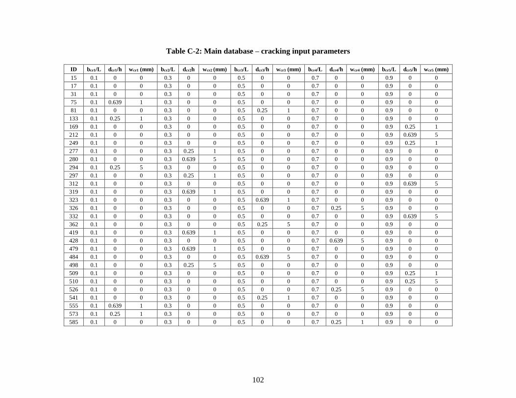
102

Table C-2: Main database – cracking input parameters

ID bcr1/L dcr1/h wcr1 (mm) bcr2/L dcr2h wcr2 (mm) bcr3/L dcr3/h wcr3 (mm) bcr4/L dcr4/h wcr4 (mm) bcr5/L dcr5/h wcr5 (mm)

15 0.1 0 0 0.3 0 0 0.5 0 0 0.7 0 0 0.9 0 0

17 0.1 0 0 0.3 0 0 0.5 0 0 0.7 0 0 0.9 0 0

31 0.1 0 0 0.3 0 0 0.5 0 0 0.7 0 0 0.9 0 0

75 0.1 0.639 1 0.3 0 0 0.5 0 0 0.7 0 0 0.9 0 0

81 0.1 0 0 0.3 0 0 0.5 0.25 1 0.7 0 0 0.9 0 0

133 0.1 0.25 1 0.3 0 0 0.5 0 0 0.7 0 0 0.9 0 0

169 0.1 0 0 0.3 0 0 0.5 0 0 0.7 0 0 0.9 0.25 1

212 0.1 0 0 0.3 0 0 0.5 0 0 0.7 0 0 0.9 0.639 5

249 0.1 0 0 0.3 0 0 0.5 0 0 0.7 0 0 0.9 0.25 1

277 0.1 0 0 0.3 0.25 1 0.5 0 0 0.7 0 0 0.9 0 0

280 0.1 0 0 0.3 0.639 5 0.5 0 0 0.7 0 0 0.9 0 0

294 0.1 0.25 5 0.3 0 0 0.5 0 0 0.7 0 0 0.9 0 0

297 0.1 0 0 0.3 0.25 1 0.5 0 0 0.7 0 0 0.9 0 0

312 0.1 0 0 0.3 0 0 0.5 0 0 0.7 0 0 0.9 0.639 5

319 0.1 0 0 0.3 0.639 1 0.5 0 0 0.7 0 0 0.9 0 0

323 0.1 0 0 0.3 0 0 0.5 0.639 1 0.7 0 0 0.9 0 0

326 0.1 0 0 0.3 0 0 0.5 0 0 0.7 0.25 5 0.9 0 0

332 0.1 0 0 0.3 0 0 0.5 0 0 0.7 0 0 0.9 0.639 5

362 0.1 0 0 0.3 0 0 0.5 0.25 5 0.7 0 0 0.9 0 0

419 0.1 0 0 0.3 0.639 1 0.5 0 0 0.7 0 0 0.9 0 0

428 0.1 0 0 0.3 0 0 0.5 0 0 0.7 0.639 5 0.9 0 0

479 0.1 0 0 0.3 0.639 1 0.5 0 0 0.7 0 0 0.9 0 0

484 0.1 0 0 0.3 0 0 0.5 0.639 5 0.7 0 0 0.9 0 0

498 0.1 0 0 0.3 0.25 5 0.5 0 0 0.7 0 0 0.9 0 0

509 0.1 0 0 0.3 0 0 0.5 0 0 0.7 0 0 0.9 0.25 1

510 0.1 0 0 0.3 0 0 0.5 0 0 0.7 0 0 0.9 0.25 5

526 0.1 0 0 0.3 0 0 0.5 0 0 0.7 0.25 5 0.9 0 0

541 0.1 0 0 0.3 0 0 0.5 0.25 1 0.7 0 0 0.9 0 0

555 0.1 0.639 1 0.3 0 0 0.5 0 0 0.7 0 0 0.9 0 0

573 0.1 0.25 1 0.3 0 0 0.5 0 0 0.7 0 0 0.9 0 0

585 0.1 0 0 0.3 0 0 0.5 0 0 0.7 0.25 1 0.9 0 0

103

ID bcr1/L dcr1/h wcr1 (mm) bcr2/L dcr2h wcr2 (mm) bcr3/L dcr3/h wcr3 (mm) bcr4/L dcr4/h wcr4 (mm) bcr5/L dcr5/h wcr5 (mm)

587 0.1 0 0 0.3 0 0 0.5 0 0 0.7 0.639 1 0.9 0 0

588 0.1 0 0 0.3 0 0 0.5 0 0 0.7 0.639 5 0.9 0 0

611 0.1 0 0 0.3 0 0 0.5 0 0 0.7 0 0 0.9 0.639 1

648 0.1 0 0 0.3 0 0 0.5 0 0 0.7 0.639 5 0.9 0 0

678 0.1 0 0 0.3 0.25 5 0.5 0 0 0.7 0 0 0.9 0 0

683 0.1 0 0 0.3 0 0 0.5 0.639 1 0.7 0 0 0.9 0 0

687 0.1 0 0 0.3 0 0 0.5 0 0 0.7 0.639 1 0.9 0 0

702 0.1 0 0 0.3 0 0 0.5 0.25 5 0.7 0 0 0.9 0 0

724 0.1 0 0 0.3 0 0 0.5 0.639 5 0.7 0 0 0.9 0 0

779 0.1 0 0 0.3 0.639 1 0.5 0 0 0.7 0 0 0.9 0 0

799 0.1 0 0 0.3 0.639 1 0.5 0 0 0.7 0 0 0.9 0 0

811 0.1 0 0 0.3 0 0 0.5 0 0 0.7 0 0 0.9 0.639 1

856 0.1 0.639 5 0.3 0 0 0.5 0 0 0.7 0 0 0.9 0 0

927 0.1 0 0 0.3 0 0 0.5 0 0 0.7 0.639 1 0.9 0 0

952 0.1 0 0 0.3 0 0 0.5 0 0 0.7 0 0 0.9 0.639 5

984 0.1 0 0 0.3 0 0 0.5 0.639 5 0.7 0 0 0.9 0 0

993 0.1 0.25 1 0.3 0 0 0.5 0 0 0.7 0 0 0.9 0 0

1033 0.1 0.25 1 0.3 0 0 0.5 0 0 0.7 0 0 0.9 0 0

1052 0.1 0 0 0.3 0 0 0.5 0 0 0.7 0 0 0.9 0.639 5

1097 0.1 0 0 0.3 0.25 1 0.5 0 0 0.7 0 0 0.9 0 0

1110 0.1 0 0 0.3 0 0 0.5 0 0 0.7 0 0 0.9 0.25 5

1129 0.1 0 0 0.3 0 0 0.5 0 0 0.7 0 0 0.9 0.25 1

1154 0.1 0.25 5 0.3 0 0 0.5 0 0 0.7 0 0 0.9 0 0

1176 0.1 0.639 5 0.3 0 0 0.5 0 0 0.7 0 0 0.9 0 0

1190 0.1 0 0 0.3 0 0 0.5 0 0 0.7 0 0 0.9 0.25 5

1250 0.1 0 0 0.3 0 0 0.5 0 0 0.7 0 0 0.9 0.25 5

1265 0.1 0 0 0.3 0 0 0.5 0 0 0.7 0.25 1 0.9 0 0

1308 0.1 0 0 0.3 0 0 0.5 0 0 0.7 0.639 5 0.9 0 0

1311 0.1 0 0 0.3 0 0 0.5 0 0 0.7 0 0 0.9 0.639 1

1340 0.1 0 0 0.3 0.639 5 0.5 0 0 0.7 0 0 0.9 0 0

1351 0.1 0 0 0.3 0 0 0.5 0 0 0.7 0 0 0.9 0.639 1

1390 0.1 0 0 0.3 0 0 0.5 0 0 0.7 0 0 0.9 0.25 5

1401 0.1 0 0 0.3 0 0 0.5 0.25 1 0.7 0 0 0.9 0 0

1407 0.1 0 0 0.3 0 0 0.5 0 0 0.7 0.639 1 0.9 0 0

1418 0.1 0 0 0.3 0.25 5 0.5 0 0 0.7 0 0 0.9 0 0

1419 0.1 0 0 0.3 0.639 1 0.5 0 0 0.7 0 0 0.9 0 0

104

ID bcr1/L dcr1/h wcr1 (mm) bcr2/L dcr2h wcr2 (mm) bcr3/L dcr3/h wcr3 (mm) bcr4/L dcr4/h wcr4 (mm) bcr5/L dcr5/h wcr5 (mm)

1462 0.1 0 0 0.3 0 0 0.5 0.25 5 0.7 0 0 0.9 0 0

1493 0.1 0.25 1 0.3 0 0 0.5 0 0 0.7 0 0 0.9 0 0

1526 0.1 0 0 0.25 0.25 5 0.5 0 0 0.7 0 0 0.9 0 0

1547 0.15 0.639 1 0.3 0 0 0.5 0 0 0.7 0 0 0.9 0 0

1556 0.1 0 0 0.2 0.639 5 0.5 0 0 0.7 0 0 0.9 0 0

1569 0.1 0 0 0.3 0 0 0.4 0.25 1 0.7 0 0 0.9 0 0

1671 0.1 0 0 0.3 0 0 0.45 0.639 1 0.7 0 0 0.9 0 0

1693 0.1 0 0 0.4 0.25 1 0.5 0 0 0.7 0 0 0.9 0 0

1709 0.2 0.25 1 0.3 0 0 0.5 0 0 0.7 0 0 0.9 0 0

1710 0.2 0.25 5 0.3 0 0 0.5 0 0 0.7 0 0 0.9 0 0

1714 0.1 0 0 0.2 0.25 5 0.5 0 0 0.7 0 0 0.9 0 0

1732 0.1 0 0 0.3 0 0 0.4 0.639 5 0.7 0 0 0.9 0 0

1745 0.1 0 0 0.2 0.25 1 0.5 0 0 0.7 0 0 0.9 0 0

1769 0.15 0.25 1 0.3 0 0 0.5 0 0 0.7 0 0 0.9 0 0

1840 0.2 0.639 5 0.3 0 0 0.5 0 0 0.7 0 0 0.9 0 0

1863 0.1 0 0 0.3 0 0 0.45 0.639 1 0.7 0 0 0.9 0 0

1875 0.1 0 0 0.2 0.639 1 0.5 0 0 0.7 0 0 0.9 0 0

1881 0.1 0 0 0.35 0.25 1 0.5 0 0 0.7 0 0 0.9 0 0

1909 0.1 0 0 0.25 0.25 1 0.5 0 0 0.7 0 0 0.9 0 0

1911 0.1 0 0 0.25 0.639 1 0.5 0 0 0.7 0 0 0.9 0 0

1939 0.1 0 0 0.2 0.639 1 0.5 0 0 0.7 0 0 0.9 0 0

1973 0.1 0 0 0.25 0.25 1 0.5 0 0 0.7 0 0 0.9 0 0

2075 0.1 0 0 0.35 0.639 1 0.5 0 0 0.7 0 0 0.9 0 0

2086 0.1 0 0 0.3 0 0 0.45 0.25 5 0.7 0 0 0.9 0 0

2095 0.2 0.639 1 0.3 0 0 0.5 0 0 0.7 0 0 0.9 0 0

2114 0.1 0 0 0.3 0 0 0.4 0.25 5 0.7 0 0 0.9 0 0

2126 0.2 0.25 5 0.3 0 0 0.5 0 0 0.7 0 0 0.9 0 0

2135 0.1 0 0 0.25 0.639 1 0.5 0 0 0.7 0 0 0.9 0 0

2178 0.1 0 0 0.3 0 0 0.4 0.25 5 0.7 0 0 0.9 0 0

2187 0.15 0.639 1 0.3 0 0 0.5 0 0 0.7 0 0 0.9 0 0

2204 0.1 0 0 0.35 0.639 5 0.5 0 0 0.7 0 0 0.9 0 0

2236 0.1 0 0 0.35 0.639 5 0.5 0 0 0.7 0 0 0.9 0 0

2241 0.1 0 0 0.3 0 0 0.4 0.25 1 0.7 0 0 0.9 0 0

2267 0.1 0 0 0.35 0.639 1 0.5 0 0 0.7 0 0 0.9 0 0

2270 0.1 0 0 0.4 0.25 5 0.5 0 0 0.7 0 0 0.9 0 0

2330 0.1 0 0 0.35 0.25 5 0.5 0 0 0.7 0 0 0.9 0 0

105

ID bcr1/L dcr1/h wcr1 (mm) bcr2/L dcr2h wcr2 (mm) bcr3/L dcr3/h wcr3 (mm) bcr4/L dcr4/h wcr4 (mm) bcr5/L dcr5/h wcr5 (mm)

2358 0.1 0 0 0.25 0.25 5 0.5 0 0 0.7 0 0 0.9 0 0

2359 0.1 0 0 0.25 0.639 1 0.5 0 0 0.7 0 0 0.9 0 0

2371 0.1 0 0 0.3 0 0 0.4 0.639 1 0.7 0 0 0.9 0 0

2396 0.1 0 0 0.35 0.639 5 0.5 0 0 0.7 0 0 0.9 0 0

2402 0.1 0 0 0.3 0 0 0.4 0.25 5 0.7 0 0 0.9 0 0

2429 0.1 0 0 0.4 0.25 1 0.5 0 0 0.7 0 0 0.9 0 0

2435 0.1 0 0 0.3 0 0 0.4 0.639 1 0.7 0 0 0.9 0 0

2459 0.1 0 0 0.35 0.639 1 0.5 0 0 0.7 0 0 0.9 0 0

2465 0.1 0 0 0.3 0 0 0.4 0.25 1 0.7 0 0 0.9 0 0

2482 0.1 0 0 0.2 0.25 5 0.5 0 0 0.7 0 0 0.9 0 0

2508 0.15 0.639 5 0.3 0 0 0.5 0 0 0.7 0 0 0.9 0 0

2546 0.1 0 0 0.2 0.25 5 0.5 0 0 0.7 0 0 0.9 0 0

2569 0.15 0.25 1 0.3 0 0 0.5 0 0 0.7 0 0 0.9 0 0

2596 0.1 0 0 0.3 0 0 0.4 0.639 5 0.7 0 0 0.9 0 0

2601 0.15 0.25 1 0.3 0 0 0.5 0 0 0.7 0 0 0.9 0 0

2604 0.15 0.639 5 0.3 0 0 0.5 0 0 0.7 0 0 0.9 0 0

2612 0.1 0 0 0.2 0.639 5 0.5 0 0 0.7 0 0 0.9 0 0

2683 0.1 0 0 0.35 0.639 1 0.5 0 0 0.7 0 0 0.9 0 0

2692 0.1 0 0 0.3 0 0 0.4 0.639 5 0.7 0 0 0.9 0 0

2733 0.2 0.25 1 0.3 0 0 0.5 0 0 0.7 0 0 0.9 0 0

2746 0.1 0 0 0.35 0.25 5 0.5 0 0 0.7 0 0 0.9 0 0

2779 0.1 0 0 0.35 0.639 1 0.5 0 0 0.7 0 0 0.9 0 0

2780 0.1 0 0 0.35 0.639 5 0.5 0 0 0.7 0 0 0.9 0 0

2784 0.1 0 0 0.4 0.639 5 0.5 0 0 0.7 0 0 0.9 0 0

2795 0.15 0.639 1 0.3 0 0 0.5 0 0 0.7 0 0 0.9 0 0

2798 0.2 0.25 5 0.3 0 0 0.5 0 0 0.7 0 0 0.9 0 0

2812 0.1 0 0 0.35 0.639 5 0.5 0 0 0.7 0 0 0.9 0 0

2815 0.1 0 0 0.4 0.639 1 0.5 0 0 0.7 0 0 0.9 0 0

2856 0.1 0 0 0.3 0 0 0.45 0.639 5 0.7 0 0 0.9 0 0

2913 0.1 0 0 0.3 0 0 0.4 0.25 1 0.7 0 0 0.9 0 0

2921 0.15 0.25 1 0.3 0 0 0.5 0 0 0.7 0 0 0.9 0 0

2925 0.2 0.25 1 0.3 0 0 0.5 0 0 0.7 0 0 0.9 0 0

2931 0.1 0 0 0.2 0.639 1 0.5 0 0 0.7 0 0 0.9 0 0

2954 0.15 0.25 5 0.3 0 0 0.5 0 0 0.7 0 0 0.9 0 0

2996 0.1 0 0 0.2 0.639 5 0.5 0 0 0.7 0 0 0.9 0 0

3049 0.15 0.25 1 0.3 0 0 0.5 0 0 0.7 0 0 0.9 0 0

106

ID bcr1/L dcr1/h wcr1 (mm) bcr2/L dcr2h wcr2 (mm) bcr3/L dcr3/h wcr3 (mm) bcr4/L dcr4/h wcr4 (mm) bcr5/L dcr5/h wcr5 (mm)

3052 0.15 0.639 5 0.3 0 0 0.5 0 0 0.7 0 0 0.9 0 0

3093 0.1 0 0 0.25 0.25 1 0.5 0 0 0.7 0 0 0.9 0 0

3109 0.1 0 0 0.3 0 0 0.45 0.25 1 0.7 0 0 0.9 0 0

3290 0.1 0 0 0.35 0.25 5 0.5 0 0 0.7 0 0 0.9 0 0

3299 0.1 0 0 0.3 0 0 0.4 0.639 1 0.7 0 0 0.9 0 0

3308 0.15 0.639 5 0.3 0 0 0.5 0 0 0.7 0 0 0.9 0 0

3313 0.1 0 0 0.2 0.25 1 0.5 0 0 0.7 0 0 0.9 0 0

3322 0.1 0 0 0.35 0.25 5 0.5 0 0 0.7 0 0 0.9 0 0

3337 0.15 0.25 1 0.3 0 0 0.5 0 0 0.7 0 0 0.9 0 0

3338 0.15 0.25 5 0.3 0 0 0.5 0 0 0.7 0 0 0.9 0 0

3382 0.1 0 0 0.25 0.25 5 0.5 0 0 0.7 0 0 0.9 0 0

3404 0.15 0.639 5 0.3 0 0 0.5 0 0 0.7 0 0 0.9 0 0

3413 0.1 0 0 0.25 0.25 1 0.5 0 0 0.7 0 0 0.9 0 0

3509 0.1 0 0 0.25 0.25 1 0.5 0 0 0.7 0 0 0.9 0 0

3525 0.1 0 0 0.3 0 0 0.45 0.25 1 0.7 0 0 0.9 0 0

3535 0.2 0.639 1 0.3 0 0 0.5 0 0 0.7 0 0 0.9 0 0

3539 0.1 0 0 0.2 0.639 1 0.5 0 0 0.7 0 0 0.9 0 0

3550 0.1 0 0 0.4 0.25 5 0.5 0 0 0.7 0 0 0.9 0 0

3602 0.1 0 0 0.2 0.25 5 0.5 0 0 0.7 0 0 0.9 0 0

3635 0.1 0 0 0.2 0.639 1 0.5 0 0 0.7 0 0 0.9 0 0

3643 0.1 0 0 0.35 0.639 1 0.5 0 0 0.7 0 0 0.9 0 0

3689 0.15 0.25 1 0.3 0 0 0.5 0 0 0.7 0 0 0.9 0 0

3716 0.1 0 0 0.3 0 0 0.4 0.639 5 0.7 0 0 0.9 0 0

3717 0.1 0 0 0.3 0 0 0.45 0.25 1 0.7 0 0 0.9 0 0

3733 0.1 0 0 0.25 0.25 1 0.5 0 0 0.7 0 0 0.9 0 0

3751 0.1 0 0 0.3 0 0 0.45 0.639 1 0.7 0 0 0.9 0 0

3764 0.1 0 0 0.2 0.639 5 0.5 0 0 0.7 0 0 0.9 0 0

3766 0.1 0 0 0.25 0.25 5 0.5 0 0 0.7 0 0 0.9 0 0

3769 0.1 0 0 0.35 0.25 1 0.5 0 0 0.7 0 0 0.9 0 0

3802 0.1 0 0 0.35 0.25 5 0.5 0 0 0.7 0 0 0.9 0 0

3828 0.1 0 0 0.3 0 0 0.5 0 0 0.6 0.639 5 0.9 0 0

3850 0.1 0 0 0.3 0 0 0.55 0.25 5 0.7 0 0 0.9 0 0

3854 0.1 0 0 0.3 0 0 0.6 0.25 5 0.7 0 0 0.9 0 0

3858 0.1 0 0 0.3 0 0 0.5 0 0 0.6 0.25 5 0.9 0 0

3863 0.1 0 0 0.3 0 0 0.5 0 0 0.65 0.639 1 0.9 0 0

3882 0.1 0 0 0.3 0 0 0.55 0.25 5 0.7 0 0 0.9 0 0

107

ID bcr1/L dcr1/h wcr1 (mm) bcr2/L dcr2h wcr2 (mm) bcr3/L dcr3/h wcr3 (mm) bcr4/L dcr4/h wcr4 (mm) bcr5/L dcr5/h wcr5 (mm)

3900 0.1 0 0 0.3 0 0 0.5 0 0 0.75 0.639 5 0.9 0 0

3944 0.1 0 0 0.3 0 0 0.5 0 0 0.7 0 0 0.85 0.639 5

4006 0.1 0 0 0.3 0 0 0.5 0 0 0.7 0 0 0.85 0.25 5

4015 0.1 0 0 0.3 0 0 0.6 0.639 1 0.7 0 0 0.9 0 0

4035 0.1 0 0 0.3 0 0 0.5 0 0 0.7 0 0 0.8 0.639 1

4090 0.1 0 0 0.3 0 0 0.5 0 0 0.75 0.25 5 0.9 0 0

4133 0.1 0 0 0.3 0 0 0.5 0 0 0.7 0 0 0.85 0.25 1

4156 0.1 0 0 0.3 0 0 0.5 0 0 0.75 0.639 5 0.9 0 0

4169 0.1 0 0 0.3 0 0 0.55 0.25 1 0.7 0 0 0.9 0 0

4177 0.1 0 0 0.3 0 0 0.5 0 0 0.6 0.25 1 0.9 0 0

4195 0.1 0 0 0.3 0 0 0.5 0 0 0.7 0 0 0.8 0.639 1

4206 0.1 0 0 0.3 0 0 0.6 0.25 5 0.7 0 0 0.9 0 0

4227 0.1 0 0 0.3 0 0 0.5 0 0 0.7 0 0 0.8 0.639 1

4266 0.1 0 0 0.3 0 0 0.55 0.25 5 0.7 0 0 0.9 0 0

4273 0.1 0 0 0.3 0 0 0.5 0 0 0.6 0.25 1 0.9 0 0

4275 0.1 0 0 0.3 0 0 0.5 0 0 0.6 0.639 1 0.9 0 0

4276 0.1 0 0 0.3 0 0 0.5 0 0 0.6 0.639 5 0.9 0 0

4306 0.1 0 0 0.3 0 0 0.5 0 0 0.6 0.25 5 0.9 0 0

4333 0.1 0 0 0.3 0 0 0.6 0.25 1 0.7 0 0 0.9 0 0

4335 0.1 0 0 0.3 0 0 0.6 0.639 1 0.7 0 0 0.9 0 0

4337 0.1 0 0 0.3 0 0 0.5 0 0 0.6 0.25 1 0.9 0 0

4364 0.1 0 0 0.3 0 0 0.55 0.639 5 0.7 0 0 0.9 0 0

4377 0.1 0 0 0.3 0 0 0.5 0 0 0.75 0.25 1 0.9 0 0

4435 0.1 0 0 0.3 0 0 0.5 0 0 0.6 0.639 1 0.9 0 0

4470 0.1 0 0 0.3 0 0 0.5 0 0 0.65 0.25 5 0.9 0 0

4530 0.1 0 0 0.3 0 0 0.5 0 0 0.6 0.25 5 0.9 0 0

4584 0.1 0 0 0.3 0 0 0.5 0 0 0.7 0 0 0.85 0.639 5

4594 0.1 0 0 0.3 0 0 0.5 0 0 0.6 0.25 5 0.9 0 0

4619 0.1 0 0 0.3 0 0 0.55 0.639 1 0.7 0 0 0.9 0 0

4642 0.1 0 0 0.3 0 0 0.5 0 0 0.7 0 0 0.8 0.25 5

4719 0.1 0 0 0.3 0 0 0.6 0.639 1 0.7 0 0 0.9 0 0

4720 0.1 0 0 0.3 0 0 0.6 0.639 5 0.7 0 0 0.9 0 0

4745 0.1 0 0 0.3 0 0 0.55 0.25 1 0.7 0 0 0.9 0 0

4750 0.1 0 0 0.3 0 0 0.6 0.25 5 0.7 0 0 0.9 0 0

4765 0.1 0 0 0.3 0 0 0.5 0 0 0.8 0.25 1 0.9 0 0

4805 0.1 0 0 0.3 0 0 0.5 0 0 0.7 0 0 0.85 0.25 1

108

ID bcr1/L dcr1/h wcr1 (mm) bcr2/L dcr2h wcr2 (mm) bcr3/L dcr3/h wcr3 (mm) bcr4/L dcr4/h wcr4 (mm) bcr5/L dcr5/h wcr5 (mm)

4834 0.1 0 0 0.3 0 0 0.5 0 0 0.7 0 0 0.8 0.25 5

4843 0.1 0 0 0.3 0 0 0.55 0.639 1 0.7 0 0 0.9 0 0

4850 0.1 0 0 0.3 0 0 0.5 0 0 0.6 0.25 5 0.9 0 0

4868 0.1 0 0 0.3 0 0 0.5 0 0 0.7 0 0 0.8 0.639 5

4884 0.1 0 0 0.3 0 0 0.5 0 0 0.6 0.639 5 0.9 0 0

4942 0.1 0 0 0.3 0 0 0.6 0.25 5 0.7 0 0 0.9 0 0

4950 0.1 0 0 0.3 0 0 0.5 0 0 0.65 0.25 5 0.9 0 0

4967 0.1 0 0 0.3 0 0 0.5 0 0 0.7 0 0 0.85 0.639 1

4972 0.1 0 0 0.3 0 0 0.55 0.639 5 0.7 0 0 0.9 0 0

4988 0.1 0 0 0.3 0 0 0.5 0 0 0.75 0.639 5 0.9 0 0

5016 0.1 0 0 0.3 0 0 0.5 0 0 0.65 0.639 5 0.9 0 0

5036 0.1 0 0 0.3 0 0 0.55 0.639 5 0.7 0 0 0.9 0 0

5043 0.1 0 0 0.3 0 0 0.5 0 0 0.6 0.639 1 0.9 0 0

5060 0.1 0 0 0.3 0 0 0.5 0 0 0.7 0 0 0.8 0.639 5

5080 0.1 0 0 0.3 0 0 0.5 0 0 0.65 0.639 5 0.9 0 0

5091 0.1 0 0 0.3 0 0 0.5 0 0 0.7 0 0 0.8 0.639 1

5099 0.1 0 0 0.3 0 0 0.55 0.639 1 0.7 0 0 0.9 0 0

5121 0.1 0 0 0.3 0 0 0.5 0 0 0.7 0 0 0.8 0.25 1

5135 0.1 0 0 0.3 0 0 0.6 0.639 1 0.7 0 0 0.9 0 0

5184 0.1 0 0 0.3 0 0 0.5 0 0 0.8 0.639 5 0.9 0 0

5207 0.1 0 0 0.3 0 0 0.5 0 0 0.65 0.639 1 0.9 0 0

5225 0.1 0 0 0.3 0 0 0.55 0.25 1 0.7 0 0 0.9 0 0

5258 0.1 0 0 0.3 0 0 0.55 0.25 5 0.7 0 0 0.9 0 0

5259 0.1 0 0 0.3 0 0 0.55 0.639 1 0.7 0 0 0.9 0 0

5291 0.1 0 0 0.3 0 0 0.55 0.639 1 0.7 0 0 0.9 0 0

5297 0.1 0 0 0.3 0 0 0.5 0 0 0.6 0.25 1 0.9 0 0

5334 0.1 0 0 0.3 0 0 0.5 0 0 0.65 0.25 5 0.9 0 0

5379 0.1 0 0 0.3 0 0 0.5 0 0 0.7 0 0 0.8 0.639 1

5448 0.1 0 0 0.3 0 0 0.5 0 0 0.7 0 0 0.85 0.639 5

5462 0.1 0 0 0.3 0 0 0.5 0 0 0.65 0.25 5 0.9 0 0

5491 0.1 0 0 0.3 0 0 0.5 0 0 0.6 0.639 1 0.9 0 0

5499 0.1 0 0 0.3 0 0 0.5 0 0 0.75 0.639 1 0.9 0 0

5546 0.1 0 0 0.3 0 0 0.55 0.25 5 0.7 0 0 0.9 0 0

5594 0.1 0 0 0.3 0 0 0.5 0 0 0.75 0.25 5 0.9 0 0

5597 0.1 0 0 0.3 0 0 0.5 0 0 0.8 0.25 1 0.9 0 0

5605 0.1 0 0 0.3 0 0 0.5 0 0 0.7 0 0 0.85 0.25 1

109

ID bcr1/L dcr1/h wcr1 (mm) bcr2/L dcr2h wcr2 (mm) bcr3/L dcr3/h wcr3 (mm) bcr4/L dcr4/h wcr4 (mm) bcr5/L dcr5/h wcr5 (mm)

5659 0.1 0 0 0.3 0 0 0.5 0 0 0.75 0.639 1 0.9 0 0

5660 0.1 0 0 0.3 0 0 0.5 0 0 0.75 0.639 5 0.9 0 0

5675 0.1 0 0 0.3 0 0 0.55 0.639 1 0.7 0 0 0.9 0 0

5691 0.1 0 0 0.3 0 0 0.5 0 0 0.75 0.639 1 0.9 0 0

5735 0.1 0 0 0.3 0 0 0.5 0 0 0.7 0 0 0.85 0.639 1

5793 0.1 0 0 0.3 0 0 0.5 0 0 0.7 0 0 0.8 0.25 1

5803 0.1 0 0 0.3 0 0 0.55 0.639 1 0.7 0 0 0.9 0 0

5825 0.1 0 0 0.3 0 0 0.5 0 0 0.7 0 0 0.8 0.25 1

5834 0.1 0 0 0.3 0 0 0.55 0.25 5 0.7 0 0 0.9 0 0

5842 0.1 0 0 0.3 0 0 0.5 0 0 0.6 0.25 5 0.9 0 0

5877 0.1 0 0 0.3 0 0 0.5 0 0 0.65 0.25 1 0.9 0 0

5932 0.1 0 0 0.3 0 0 0.55 0.639 5 0.7 0 0 0.9 0 0

5938 0.1 0 0 0.3 0 0 0.5 0 0 0.6 0.25 5 0.9 0 0

5963 0.1 0 0 0.3 0 0 0.55 0.639 1 0.7 0 0 0.9 0 0

5980 0.1 0 0 0.3 0 0 0.5 0 0 0.75 0.639 5 0.9 0 0

5993 0.1 0 0 0.3 0 0 0.55 0.25 1 0.7 0 0 0.9 0 0

5998 0.1 0 0 0.3 0 0 0.6 0.25 5 0.7 0 0 0.9 0 0

6026 0.1 0 0 0.3 0 0 0.55 0.25 5 0.7 0 0 0.9 0 0

6082 0.1 0 0 0.3 0 0 0.5 0 0 0.7 0 0 0.8 0.25 5

6127 0.1 0 0 0.3 0 0 0.5 0 0 0.7 0 0 0.94 0.639 1

6173 0.1 0 0 0.3 0 0 0.5 0 0 0.7 0 0 0.94 0.25 1

6210 0.06 0.25 5 0.3 0 0 0.5 0 0 0.7 0 0 0.9 0 0

6216 0.1 0 0 0.3 0 0 0.5 0 0 0.7 0 0 0.94 0.639 5

6272 0.1 0 0 0.3 0 0 0.5 0 0 0.7 0 0 0.94 0.639 5

6282 0.06 0.25 5 0.3 0 0 0.5 0 0 0.7 0 0 0.9 0 0

6284 0.06 0.639 5 0.3 0 0 0.5 0 0 0.7 0 0 0.9 0 0

6292 0.06 0.639 5 0.3 0 0 0.5 0 0 0.7 0 0 0.9 0 0

6309 0.1 0 0 0.3 0 0 0.5 0 0 0.7 0 0 0.94 0.25 1

6339 0.06 0.639 1 0.3 0 0 0.5 0 0 0.7 0 0 0.9 0 0

6351 0.1 0 0 0.3 0 0 0.5 0 0 0.7 0 0 0.94 0.639 1

6414 0.1 0 0 0.3 0 0 0.5 0 0 0.7 0 0 0.94 0.25 5

6418 0.06 0.25 5 0.3 0 0 0.5 0 0 0.7 0 0 0.9 0 0

6425 0.06 0.25 1 0.3 0 0 0.5 0 0 0.7 0 0 0.9 0 0

6460 0.06 0.639 5 0.3 0 0 0.5 0 0 0.7 0 0 0.9 0 0

6464 0.1 0 0 0.3 0 0 0.5 0 0 0.7 0 0 0.94 0.639 5

6496 0.1 0 0 0.3 0 0 0.5 0 0 0.7 0 0 0.94 0.639 5

110

ID bcr1/L dcr1/h wcr1 (mm) bcr2/L dcr2h wcr2 (mm) bcr3/L dcr3/h wcr3 (mm) bcr4/L dcr4/h wcr4 (mm) bcr5/L dcr5/h wcr5 (mm)

6516 0.06 0.639 5 0.3 0 0 0.5 0 0 0.7 0 0 0.9 0 0

6521 0.06 0.25 1 0.3 0 0 0.5 0 0 0.7 0 0 0.9 0 0

6544 0.1 0 0 0.3 0 0 0.5 0 0 0.7 0 0 0.94 0.639 5

6561 0.06 0.25 1 0.3 0 0 0.5 0 0 0.7 0 0 0.9 0 0

6578 0.06 0.25 5 0.3 0 0 0.5 0 0 0.7 0 0 0.9 0 0

6606 0.1 0 0 0.3 0 0 0.5 0 0 0.7 0 0 0.94 0.25 5

6625 0.06 0.25 1 0.3 0 0 0.5 0 0 0.7 0 0 0.9 0 0

6656 0.1 0 0 0.3 0 0 0.5 0 0 0.7 0 0 0.94 0.639 5

6681 0.06 0.25 1 0.3 0 0 0.5 0 0 0.7 0 0 0.9 0 0

6697 0.1 0.25 1 0.3 0.25 1 0.5 0.25 1 0.7 0.25 1 0.9 0.25 1

6712 0.1 0.639 1 0.3 0.639 1 0.5 0.639 1 0.7 0.639 1 0.9 0.639 1

6720 0.1 0.5 5 0.3 0.5 5 0.5 0.5 5 0.7 0.5 5 0.9 0.5 5

6741 0.1 0.639 5 0.3 0.639 5 0.5 0.639 5 0.7 0.639 5 0.9 0.639 5

6757 0.1 0.639 1 0.3 0.639 1 0.5 0.639 1 0.7 0.639 1 0.9 0.639 1

6781 0.1 0.5 1 0.3 0.5 1 0.5 0.5 1 0.7 0.5 1 0.9 0.5 1

6812 0.1 0.639 2.5 0.3 0.639 2.5 0.5 0.639 2.5 0.7 0.639 2.5 0.9 0.639 2.5

6856 0.1 0.639 1 0.3 0.639 1 0.5 0.639 1 0.7 0.639 1 0.9 0.639 1

6909 0.1 0.5 5 0.3 0.5 5 0.5 0.5 5 0.7 0.5 5 0.9 0.5 5

6915 0.1 0.25 5 0.3 0.25 5 0.5 0.25 5 0.7 0.25 5 0.9 0.25 5

6933 0.1 0.25 5 0.3 0.25 5 0.5 0.25 5 0.7 0.25 5 0.9 0.25 5

6943 0.1 0.5 1 0.3 0.5 1 0.5 0.5 1 0.7 0.5 1 0.9 0.5 1

7005 0.1 0.25 5 0.3 0.25 5 0.5 0.25 5 0.7 0.25 5 0.9 0.25 5

7048 0.1 0.25 1 0.3 0.25 1 0.5 0.25 1 0.7 0.25 1 0.9 0.25 1

7059 0.1 0.25 5 0.3 0.25 5 0.5 0.25 5 0.7 0.25 5 0.9 0.25 5

7074 0.1 0.639 5 0.3 0.639 5 0.5 0.639 5 0.7 0.639 5 0.9 0.639 5

7095 0.1 0.25 5 0.3 0.25 5 0.5 0.25 5 0.7 0.25 5 0.9 0.25 5

7109 0.1 0.639 2.5 0.3 0.639 2.5 0.5 0.639 2.5 0.7 0.639 2.5 0.9 0.639 2.5

7191 0.1 0.639 5 0.3 0.639 5 0.5 0.639 5 0.7 0.639 5 0.9 0.639 5

7229 0.1 0.25 2.5 0.3 0.25 2.5 0.5 0.25 2.5 0.7 0.25 2.5 0.9 0.25 2.5

7250 0.1 0.5 2.5 0.3 0.5 2.5 0.5 0.5 2.5 0.7 0.5 2.5 0.9 0.5 2.5

7264 0.1 0.25 1 0.3 0.25 1 0.5 0.25 1 0.7 0.25 1 0.9 0.25 1

7329 0.1 0.25 5 0.3 0.25 5 0.5 0.25 5 0.7 0.25 5 0.9 0.25 5

7374 0.2 0.25 5 0.4 0.25 5 0.5 0.25 5 0.6 0.25 5 0.8 0.25 5

7378 0.2 0.639 1 0.4 0.639 1 0.5 0.639 1 0.6 0.639 1 0.8 0.639 1

7379 0.2 0.639 2.5 0.4 0.639 2.5 0.5 0.639 2.5 0.6 0.639 2.5 0.8 0.639 2.5

7397 0.2 0.639 2.5 0.4 0.639 2.5 0.5 0.639 2.5 0.6 0.639 2.5 0.8 0.639 2.5

111

ID bcr1/L dcr1/h wcr1 (mm) bcr2/L dcr2h wcr2 (mm) bcr3/L dcr3/h wcr3 (mm) bcr4/L dcr4/h wcr4 (mm) bcr5/L dcr5/h wcr5 (mm)

7409 0.2 0.25 2.5 0.4 0.25 2.5 0.5 0.25 2.5 0.6 0.25 2.5 0.8 0.25 2.5

7410 0.2 0.25 5 0.4 0.25 5 0.5 0.25 5 0.6 0.25 5 0.8 0.25 5

7472 0.2 0.25 2.5 0.4 0.25 2.5 0.5 0.25 2.5 0.6 0.25 2.5 0.8 0.25 2.5

7507 0.2 0.25 1 0.4 0.25 1 0.5 0.25 1 0.6 0.25 1 0.8 0.25 1

7532 0.2 0.639 2.5 0.4 0.639 2.5 0.5 0.639 2.5 0.6 0.639 2.5 0.8 0.639 2.5

7535 0.2 0.25 2.5 0.4 0.25 2.5 0.5 0.25 2.5 0.6 0.25 2.5 0.8 0.25 2.5

7551 0.2 0.639 5 0.4 0.639 5 0.5 0.639 5 0.6 0.639 5 0.8 0.639 5

7554 0.2 0.25 5 0.4 0.25 5 0.5 0.25 5 0.6 0.25 5 0.8 0.25 5

7555 0.2 0.5 1 0.4 0.5 1 0.5 0.5 1 0.6 0.5 1 0.8 0.5 1

7567 0.2 0.639 1 0.4 0.639 1 0.5 0.639 1 0.6 0.639 1 0.8 0.639 1

7600 0.2 0.5 1 0.4 0.5 1 0.5 0.5 1 0.6 0.5 1 0.8 0.5 1

7612 0.2 0.639 1 0.4 0.639 1 0.5 0.639 1 0.6 0.639 1 0.8 0.639 1

7686 0.2 0.639 5 0.4 0.639 5 0.5 0.639 5 0.6 0.639 5 0.8 0.639 5

7688 0.2 0.25 2.5 0.4 0.25 2.5 0.5 0.25 2.5 0.6 0.25 2.5 0.8 0.25 2.5

7689 0.2 0.25 5 0.4 0.25 5 0.5 0.25 5 0.6 0.25 5 0.8 0.25 5

7690 0.2 0.5 1 0.4 0.5 1 0.5 0.5 1 0.6 0.5 1 0.8 0.5 1

7709 0.2 0.5 2.5 0.4 0.5 2.5 0.5 0.5 2.5 0.6 0.5 2.5 0.8 0.5 2.5

7710 0.2 0.5 5 0.4 0.5 5 0.5 0.5 5 0.6 0.5 5 0.8 0.5 5

7720 0.2 0.639 1 0.4 0.639 1 0.5 0.639 1 0.6 0.639 1 0.8 0.639 1

7759 0.2 0.25 1 0.4 0.25 1 0.5 0.25 1 0.6 0.25 1 0.8 0.25 1

7778 0.2 0.25 2.5 0.4 0.25 2.5 0.5 0.25 2.5 0.6 0.25 2.5 0.8 0.25 2.5

7793 0.2 0.639 2.5 0.4 0.639 2.5 0.5 0.639 2.5 0.6 0.639 2.5 0.8 0.639 2.5

7813 0.2 0.25 1 0.4 0.25 1 0.5 0.25 1 0.6 0.25 1 0.8 0.25 1

7826 0.2 0.5 2.5 0.4 0.5 2.5 0.5 0.5 2.5 0.6 0.5 2.5 0.8 0.5 2.5

7834 0.2 0.5 1 0.4 0.5 1 0.5 0.5 1 0.6 0.5 1 0.8 0.5 1

7838 0.2 0.639 2.5 0.4 0.639 2.5 0.5 0.639 2.5 0.6 0.639 2.5 0.8 0.639 2.5

7840 0.2 0.25 1 0.4 0.25 1 0.5 0.25 1 0.6 0.25 1 0.8 0.25 1

7863 0.2 0.5 5 0.4 0.5 5 0.5 0.5 5 0.6 0.5 5 0.8 0.5 5

7874 0.2 0.639 2.5 0.4 0.639 2.5 0.5 0.639 2.5 0.6 0.639 2.5 0.8 0.639 2.5

7916 0.2 0.5 2.5 0.4 0.5 2.5 0.5 0.5 2.5 0.6 0.5 2.5 0.8 0.5 2.5

7918 0.2 0.639 1 0.4 0.639 1 0.5 0.639 1 0.6 0.639 1 0.8 0.639 1

7921 0.2 0.25 1 0.4 0.25 1 0.5 0.25 1 0.6 0.25 1 0.8 0.25 1

8001 0.06 0.1 0.05 0.21 0.639 2.5 0.41 0.639 0.05 0.61 0.639 2.5 0.81 0.1 0.05

8010 0.06 0.1 2.5 0.21 0.639 2.5 0.41 0.1 2.5 0.61 0.639 0.05 0.81 0.1 0.05

8027 0.06 0.639 0.05 0.21 0.639 0.05 0.41 0.639 2.5 0.61 0.1 2.5 0.81 0.1 2.5

8028 0.06 0.639 2.5 0.21 0.639 2.5 0.41 0.639 2.5 0.61 0.1 0.05 0.81 0.1 0.05

112

ID bcr1/L dcr1/h wcr1 (mm) bcr2/L dcr2h wcr2 (mm) bcr3/L dcr3/h wcr3 (mm) bcr4/L dcr4/h wcr4 (mm) bcr5/L dcr5/h wcr5 (mm)

8075 0.19 0.1 0.05 0.21 0.639 0.05 0.59 0.639 2.5 0.61 0.639 2.5 0.94 0.1 2.5

8079 0.19 0.1 0.05 0.21 0.639 2.5 0.59 0.1 0.05 0.61 0.639 2.5 0.94 0.1 0.05

8109 0.06 0.1 0.05 0.39 0.639 2.5 0.41 0.639 0.05 0.79 0.639 2.5 0.81 0.1 0.05

8131 0.06 0.639 2.5 0.39 0.639 0.05 0.41 0.639 2.5 0.79 0.1 0.05 0.81 0.1 2.5

8132 0.06 0.639 0.05 0.39 0.639 2.5 0.41 0.639 2.5 0.79 0.1 2.5 0.81 0.1 0.05

8143 0.06 0.1 2.5 0.21 0.639 0.05 0.41 0.639 2.5 0.61 0.639 0.05 0.81 0.1 2.5

8159 0.06 0.639 0.05 0.21 0.1 0.05 0.41 0.1 2.5 0.61 0.1 2.5 0.81 0.639 2.5

8184 0.19 0.1 2.5 0.39 0.639 2.5 0.59 0.639 2.5 0.79 0.639 0.05 0.94 0.1 0.05

8192 0.19 0.639 0.05 0.39 0.1 2.5 0.59 0.1 2.5 0.79 0.1 2.5 0.94 0.639 0.05

8198 0.19 0.1 0.05 0.39 0.1 2.5 0.59 0.639 2.5 0.79 0.639 2.5 0.94 0.639 0.05

8223 0.19 0.1 0.05 0.21 0.639 2.5 0.59 0.1 0.05 0.61 0.639 2.5 0.94 0.1 0.05

8224 0.19 0.1 2.5 0.21 0.639 0.05 0.59 0.1 0.05 0.61 0.639 0.05 0.94 0.1 2.5

8264 0.06 0.639 0.05 0.39 0.1 2.5 0.41 0.1 2.5 0.79 0.1 2.5 0.81 0.639 0.05

8271 0.06 0.1 0.05 0.39 0.1 2.5 0.41 0.639 0.05 0.79 0.639 2.5 0.81 0.639 0.05

8328 0.19 0.1 2.5 0.39 0.639 2.5 0.59 0.639 2.5 0.79 0.639 0.05 0.94 0.1 0.05

8371 0.19 0.639 2.5 0.21 0.1 0.05 0.59 0.1 2.5 0.61 0.1 0.05 0.94 0.639 2.5

8383 0.19 0.639 2.5 0.21 0.639 0.05 0.59 0.639 2.5 0.61 0.1 0.05 0.94 0.1 2.5

8392 0.06 0.639 2.5 0.39 0.1 0.05 0.41 0.639 0.05 0.79 0.1 0.05 0.81 0.639 2.5

8411 0.06 0.639 0.05 0.39 0.1 0.05 0.41 0.1 2.5 0.79 0.1 2.5 0.81 0.639 2.5

8451 0.06 0.1 0.05 0.21 0.1 2.5 0.41 0.639 0.05 0.61 0.639 2.5 0.81 0.639 0.05

8473 0.19 0.1 2.5 0.39 0.639 0.05 0.59 0.1 2.5 0.79 0.639 0.05 0.94 0.1 2.5

8513 0.19 0.1 0.05 0.21 0.639 0.05 0.59 0.1 2.5 0.61 0.639 2.5 0.94 0.1 2.5

8528 0.19 0.639 0.05 0.21 0.639 2.5 0.59 0.639 2.5 0.61 0.1 2.5 0.94 0.1 0.05

8536 0.06 0.639 2.5 0.39 0.1 0.05 0.41 0.639 0.05 0.79 0.1 0.05 0.81 0.639 2.5

8545 0.06 0.1 2.5 0.39 0.639 0.05 0.41 0.1 2.5 0.79 0.639 0.05 0.81 0.1 2.5

8561 0.06 0.1 0.05 0.39 0.1 0.05 0.41 0.639 2.5 0.79 0.639 2.5 0.81 0.639 2.5

8587 0.06 0.639 2.5 0.21 0.1 0.05 0.41 0.1 2.5 0.61 0.1 0.05 0.81 0.639 2.5

8595 0.06 0.1 0.05 0.21 0.1 2.5 0.41 0.639 0.05 0.61 0.639 2.5 0.81 0.639 0.05

8597 0.06 0.1 0.05 0.21 0.1 0.05 0.41 0.639 2.5 0.61 0.639 2.5 0.81 0.639 2.5

8623 0.19 0.639 2.5 0.39 0.1 0.05 0.59 0.1 2.5 0.79 0.1 0.05 0.94 0.639 2.5

8667 0.19 0.1 0.05 0.21 0.1 2.5 0.59 0.639 0.05 0.61 0.639 2.5 0.94 0.639 0.05

8695 0.06 0.639 2.5 0.39 0.1 0.05 0.41 0.1 2.5 0.79 0.1 0.05 0.81 0.639 2.5

8704 0.06 0.1 2.5 0.39 0.1 0.05 0.41 0.639 0.05 0.79 0.639 0.05 0.81 0.639 2.5

8728 0.06 0.1 2.5 0.21 0.639 0.05 0.41 0.1 0.05 0.61 0.639 0.05 0.81 0.1 2.5

8769 0.19 0.639 0.05 0.39 0.1 2.5 0.59 0.1 0.05 0.79 0.1 2.5 0.94 0.639 0.05

8779 0.19 0.639 2.5 0.39 0.639 0.05 0.59 0.639 2.5 0.79 0.1 0.05 0.94 0.1 2.5

113

ID bcr1/L dcr1/h wcr1 (mm) bcr2/L dcr2h wcr2 (mm) bcr3/L dcr3/h wcr3 (mm) bcr4/L dcr4/h wcr4 (mm) bcr5/L dcr5/h wcr5 (mm)

8782 0.19 0.639 2.5 0.39 0.639 0.05 0.59 0.639 0.05 0.79 0.1 0.05 0.94 0.1 2.5

8825 0.06 0.639 0.05 0.39 0.1 0.05 0.41 0.639 2.5 0.79 0.1 2.5 0.81 0.639 2.5

8831 0.06 0.1 0.05 0.39 0.639 0.05 0.41 0.639 2.5 0.79 0.639 2.5 0.81 0.1 2.5

8844 0.06 0.639 2.5 0.39 0.1 2.5 0.41 0.1 2.5 0.79 0.1 0.05 0.81 0.639 0.05

8867 0.06 0.1 0.05 0.21 0.639 0.05 0.41 0.639 2.5 0.61 0.639 2.5 0.81 0.1 2.5

8880 0.06 0.639 2.5 0.21 0.1 2.5 0.41 0.1 2.5 0.61 0.1 0.05 0.81 0.639 0.05

8893 0.19 0.639 2.5 0.39 0.1 0.05 0.59 0.639 2.5 0.79 0.1 0.05 0.94 0.639 2.5

8918 0.19 0.1 0.05 0.39 0.1 2.5 0.59 0.639 2.5 0.79 0.639 2.5 0.94 0.639 0.05

8945 0.19 0.1 0.05 0.21 0.639 0.05 0.59 0.1 2.5 0.61 0.639 2.5 0.94 0.1 2.5

8976 0.06 0.1 2.5 0.39 0.639 2.5 0.41 0.639 2.5 0.79 0.639 0.05 0.81 0.1 0.05

9009 0.06 0.1 0.05 0.21 0.639 2.5 0.41 0.639 0.05 0.61 0.639 2.5 0.81 0.1 0.05

9026 0.06 0.1 0.05 0.21 0.1 2.5 0.41 0.639 2.5 0.61 0.639 2.5 0.81 0.639 0.05

9053 0.19 0.1 0.05 0.39 0.639 0.05 0.59 0.1 2.5 0.79 0.639 2.5 0.94 0.1 2.5

9075 0.19 0.639 0.05 0.21 0.1 2.5 0.59 0.639 0.05 0.61 0.1 2.5 0.94 0.639 0.05

9118 0.06 0.1 2.5 0.39 0.639 0.05 0.41 0.639 0.05 0.79 0.639 0.05 0.81 0.1 2.5

9123 0.06 0.1 0.05 0.39 0.639 2.5 0.41 0.1 0.05 0.79 0.639 2.5 0.81 0.1 0.05

9163 0.06 0.639 2.5 0.21 0.1 0.05 0.41 0.1 2.5 0.61 0.1 0.05 0.81 0.639 2.5

9182 0.19 0.639 0.05 0.39 0.1 2.5 0.59 0.639 2.5 0.79 0.1 2.5 0.94 0.639 0.05

9188 0.19 0.1 0.05 0.39 0.639 2.5 0.59 0.639 2.5 0.79 0.639 2.5 0.94 0.1 0.05

9201 0.19 0.639 0.05 0.39 0.1 2.5 0.59 0.1 0.05 0.79 0.1 2.5 0.94 0.639 0.05

9208 0.19 0.1 2.5 0.39 0.1 0.05 0.59 0.639 0.05 0.79 0.639 0.05 0.94 0.639 2.5

9211 0.19 0.639 2.5 0.39 0.639 0.05 0.59 0.639 2.5 0.79 0.1 0.05 0.94 0.1 2.5

9214 0.19 0.639 2.5 0.39 0.639 0.05 0.59 0.639 0.05 0.79 0.1 0.05 0.94 0.1 2.5

9215 0.19 0.639 0.05 0.39 0.639 0.05 0.59 0.639 2.5 0.79 0.1 2.5 0.94 0.1 2.5

9295 0.06 0.1 2.5 0.21 0.639 0.05 0.41 0.639 2.5 0.61 0.639 0.05 0.81 0.1 2.5

9359 0.19 0.639 0.05 0.39 0.639 0.05 0.59 0.639 2.5 0.79 0.1 2.5 0.94 0.1 2.5

9440 0.06 0.1 0.05 0.21 0.639 2.5 0.41 0.639 2.5 0.61 0.639 2.5 0.81 0.1 0.05

9461 0.06 0.1 0.05 0.21 0.1 0.05 0.41 0.639 2.5 0.61 0.639 2.5 0.81 0.639 2.5

9526 0.19 0.639 2.5 0.21 0.1 0.05 0.59 0.1 0.05 0.61 0.1 0.05 0.94 0.639 2.5

9528 0.19 0.639 2.5 0.21 0.1 2.5 0.59 0.1 2.5 0.61 0.1 0.05 0.94 0.639 0.05

9536 0.19 0.639 0.05 0.21 0.639 2.5 0.59 0.639 2.5 0.61 0.1 2.5 0.94 0.1 0.05

9548 0.06 0.1 0.05 0.39 0.639 2.5 0.41 0.639 2.5 0.79 0.639 2.5 0.81 0.1 0.05

9599 0.06 0.639 0.05 0.21 0.1 0.05 0.41 0.1 2.5 0.61 0.1 2.5 0.81 0.639 2.5

9608 0.06 0.639 0.05 0.21 0.639 2.5 0.41 0.639 2.5 0.61 0.1 2.5 0.81 0.1 0.05

9653 0.19 0.639 0.05 0.21 0.1 0.05 0.59 0.639 2.5 0.61 0.1 2.5 0.94 0.639 2.5

9669 0.19 0.639 0.05 0.21 0.1 2.5 0.59 0.1 0.05 0.61 0.1 2.5 0.94 0.639 0.05

114

ID bcr1/L dcr1/h wcr1 (mm) bcr2/L dcr2h wcr2 (mm) bcr3/L dcr3/h wcr3 (mm) bcr4/L dcr4/h wcr4 (mm) bcr5/L dcr5/h wcr5 (mm)

9688 0.06 0.639 2.5 0.39 0.1 0.05 0.41 0.639 0.05 0.79 0.1 0.05 0.81 0.639 2.5

9694 0.06 0.1 2.5 0.39 0.639 0.05 0.41 0.639 0.05 0.79 0.639 0.05 0.81 0.1 2.5

9729 0.06 0.1 0.05 0.21 0.639 2.5 0.41 0.639 0.05 0.61 0.639 2.5 0.81 0.1 0.05

9730 0.06 0.1 2.5 0.21 0.639 0.05 0.41 0.639 0.05 0.61 0.639 0.05 0.81 0.1 2.5

9857 0.06 0.1 0.05 0.39 0.1 0.05 0.41 0.639 2.5 0.79 0.639 2.5 0.81 0.639 2.5

9882 0.06 0.1 2.5 0.21 0.639 2.5 0.41 0.1 2.5 0.61 0.639 0.05 0.81 0.1 0.05

9911 0.19 0.1 0.05 0.39 0.639 0.05 0.59 0.639 2.5 0.79 0.639 2.5 0.94 0.1 2.5

9920 0.19 0.639 0.05 0.39 0.1 2.5 0.59 0.1 2.5 0.79 0.1 2.5 0.94 0.639 0.05

10000 0.06 0.1 2.5 0.39 0.1 0.05 0.41 0.639 0.05 0.79 0.639 0.05 0.81 0.639 2.5

10003 0.06 0.639 2.5 0.39 0.639 0.05 0.41 0.639 2.5 0.79 0.1 0.05 0.81 0.1 2.5

10008 0.06 0.639 2.5 0.39 0.639 2.5 0.41 0.639 2.5 0.79 0.1 0.05 0.81 0.1 0.05

10017 0.06 0.1 0.05 0.21 0.639 2.5 0.41 0.639 0.05 0.61 0.639 2.5 0.81 0.1 0.05

10055 0.19 0.1 0.05 0.39 0.639 0.05 0.59 0.639 2.5 0.79 0.639 2.5 0.94 0.1 2.5

10116 0.19 0.639 2.5 0.21 0.639 2.5 0.59 0.639 2.5 0.61 0.1 0.05 0.94 0.1 0.05

10141 0.06 0.1 2.5 0.39 0.1 0.05 0.41 0.639 2.5 0.79 0.639 0.05 0.81 0.639 2.5

10147 0.06 0.639 2.5 0.39 0.639 0.05 0.41 0.639 2.5 0.79 0.1 0.05 0.81 0.1 2.5

10169 0.06 0.1 0.05 0.21 0.639 0.05 0.41 0.1 2.5 0.61 0.639 2.5 0.81 0.1 2.5

10196 0.19 0.1 0.05 0.39 0.639 2.5 0.59 0.639 2.5 0.79 0.639 2.5 0.94 0.1 0.05

10238 0.19 0.1 0.05 0.21 0.639 2.5 0.59 0.1 2.5 0.61 0.639 2.5 0.94 0.1 0.05

10256 0.19 0.639 0.05 0.21 0.639 2.5 0.59 0.639 2.5 0.61 0.1 2.5 0.94 0.1 0.05

10276 0.06 0.1 2.5 0.39 0.639 0.05 0.41 0.1 0.05 0.79 0.639 0.05 0.81 0.1 2.5

10303 0.1 0.1 5 0.3 0 0 0.5 0 0 0.7 0 0 0.9 0.639 0.05

10344 0.1 0 0 0.3 0.1 0.05 0.5 0 0 0.7 0.639 5 0.9 0 0

10348 0.1 0.1 0.05 0.3 0.639 5 0.5 0 0 0.7 0 0 0.9 0 0

10352 0.1 0.1 0.05 0.3 0 0 0.5 0 0 0.7 0 0 0.9 0.639 5

10375 0.1 0 0 0.3 0.1 5 0.5 0 0 0.7 0.639 0.05 0.9 0 0

10413 0.1 0.639 5 0.3 0 0 0.5 0 0 0.7 0 0 0.9 0.1 0.05

10497 0.1 0 0 0.3 0.639 5 0.5 0.1 0.05 0.7 0 0 0.9 0 0

10575 0.1 0.1 5 0.3 0.25 2.5 0.5 0 0 0.7 0.639 0.05 0.9 0 0

10596 0.1 0.1 0.05 0.3 0.25 2.5 0.5 0 0 0.7 0 0 0.9 0.639 5

10628 0.1 0.1 0.05 0.3 0.25 2.5 0.5 0 0 0.7 0 0 0.9 0.639 5

10672 0.1 0.1 0.05 0.3 0.25 2.5 0.5 0 0 0.7 0.639 5 0.9 0 0

10712 0.1 0.1 0.05 0.3 0 0 0.5 0.25 2.5 0.7 0 0 0.9 0.639 5

10741 0.1 0.639 5 0.3 0 0 0.5 0.25 2.5 0.7 0 0 0.9 0.1 0.05

10765 0.1 0.639 5 0.3 0.25 2.5 0.5 0 0 0.7 0.1 0.05 0.9 0 0

10767 0.1 0.1 5 0.3 0.25 2.5 0.5 0 0 0.7 0.639 0.05 0.9 0 0

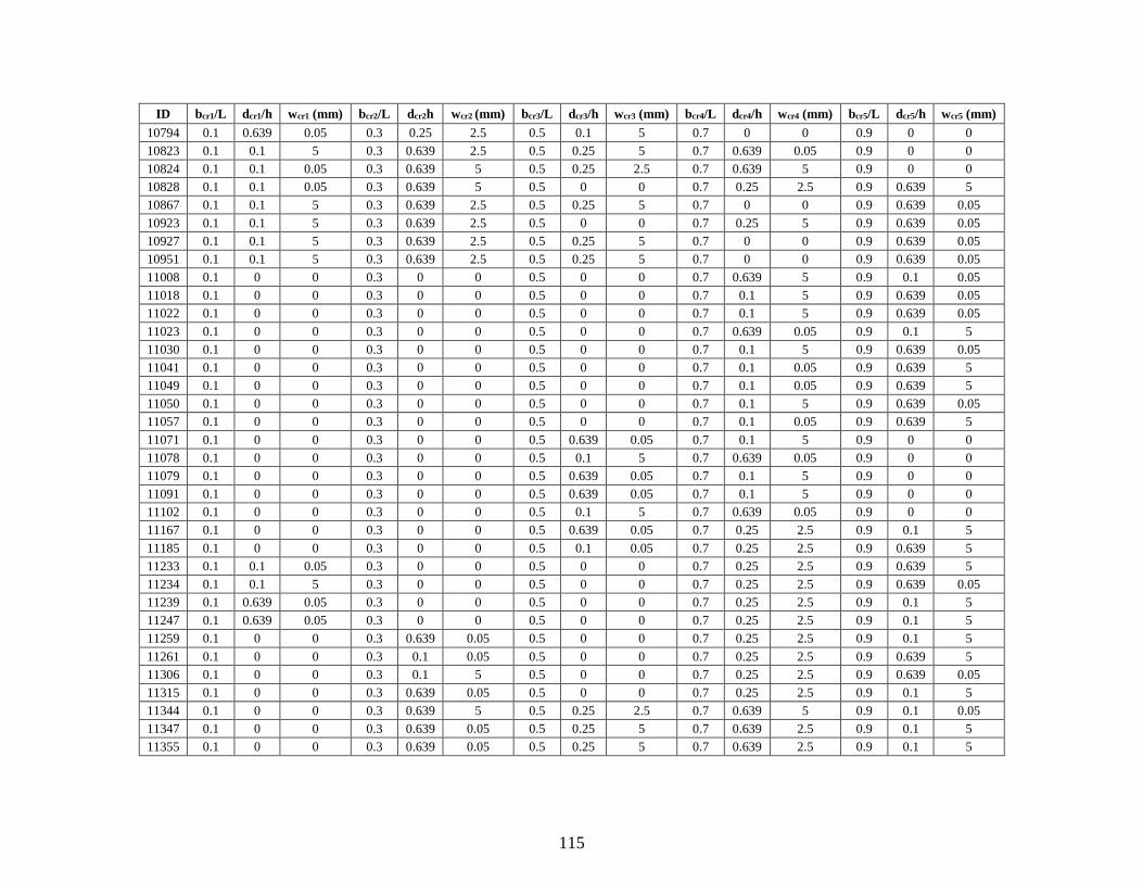
115

ID bcr1/L dcr1/h wcr1 (mm) bcr2/L dcr2h wcr2 (mm) bcr3/L dcr3/h wcr3 (mm) bcr4/L dcr4/h wcr4 (mm) bcr5/L dcr5/h wcr5 (mm)

10794 0.1 0.639 0.05 0.3 0.25 2.5 0.5 0.1 5 0.7 0 0 0.9 0 0

10823 0.1 0.1 5 0.3 0.639 2.5 0.5 0.25 5 0.7 0.639 0.05 0.9 0 0

10824 0.1 0.1 0.05 0.3 0.639 5 0.5 0.25 2.5 0.7 0.639 5 0.9 0 0

10828 0.1 0.1 0.05 0.3 0.639 5 0.5 0 0 0.7 0.25 2.5 0.9 0.639 5

10867 0.1 0.1 5 0.3 0.639 2.5 0.5 0.25 5 0.7 0 0 0.9 0.639 0.05

10923 0.1 0.1 5 0.3 0.639 2.5 0.5 0 0 0.7 0.25 5 0.9 0.639 0.05

10927 0.1 0.1 5 0.3 0.639 2.5 0.5 0.25 5 0.7 0 0 0.9 0.639 0.05

10951 0.1 0.1 5 0.3 0.639 2.5 0.5 0.25 5 0.7 0 0 0.9 0.639 0.05

11008 0.1 0 0 0.3 0 0 0.5 0 0 0.7 0.639 5 0.9 0.1 0.05

11018 0.1 0 0 0.3 0 0 0.5 0 0 0.7 0.1 5 0.9 0.639 0.05

11022 0.1 0 0 0.3 0 0 0.5 0 0 0.7 0.1 5 0.9 0.639 0.05

11023 0.1 0 0 0.3 0 0 0.5 0 0 0.7 0.639 0.05 0.9 0.1 5

11030 0.1 0 0 0.3 0 0 0.5 0 0 0.7 0.1 5 0.9 0.639 0.05

11041 0.1 0 0 0.3 0 0 0.5 0 0 0.7 0.1 0.05 0.9 0.639 5

11049 0.1 0 0 0.3 0 0 0.5 0 0 0.7 0.1 0.05 0.9 0.639 5

11050 0.1 0 0 0.3 0 0 0.5 0 0 0.7 0.1 5 0.9 0.639 0.05

11057 0.1 0 0 0.3 0 0 0.5 0 0 0.7 0.1 0.05 0.9 0.639 5

11071 0.1 0 0 0.3 0 0 0.5 0.639 0.05 0.7 0.1 5 0.9 0 0

11078 0.1 0 0 0.3 0 0 0.5 0.1 5 0.7 0.639 0.05 0.9 0 0

11079 0.1 0 0 0.3 0 0 0.5 0.639 0.05 0.7 0.1 5 0.9 0 0

11091 0.1 0 0 0.3 0 0 0.5 0.639 0.05 0.7 0.1 5 0.9 0 0

11102 0.1 0 0 0.3 0 0 0.5 0.1 5 0.7 0.639 0.05 0.9 0 0

11167 0.1 0 0 0.3 0 0 0.5 0.639 0.05 0.7 0.25 2.5 0.9 0.1 5

11185 0.1 0 0 0.3 0 0 0.5 0.1 0.05 0.7 0.25 2.5 0.9 0.639 5

11233 0.1 0.1 0.05 0.3 0 0 0.5 0 0 0.7 0.25 2.5 0.9 0.639 5

11234 0.1 0.1 5 0.3 0 0 0.5 0 0 0.7 0.25 2.5 0.9 0.639 0.05

11239 0.1 0.639 0.05 0.3 0 0 0.5 0 0 0.7 0.25 2.5 0.9 0.1 5

11247 0.1 0.639 0.05 0.3 0 0 0.5 0 0 0.7 0.25 2.5 0.9 0.1 5

11259 0.1 0 0 0.3 0.639 0.05 0.5 0 0 0.7 0.25 2.5 0.9 0.1 5

11261 0.1 0 0 0.3 0.1 0.05 0.5 0 0 0.7 0.25 2.5 0.9 0.639 5

11306 0.1 0 0 0.3 0.1 5 0.5 0 0 0.7 0.25 2.5 0.9 0.639 0.05

11315 0.1 0 0 0.3 0.639 0.05 0.5 0 0 0.7 0.25 2.5 0.9 0.1 5

11344 0.1 0 0 0.3 0.639 5 0.5 0.25 2.5 0.7 0.639 5 0.9 0.1 0.05

11347 0.1 0 0 0.3 0.639 0.05 0.5 0.25 5 0.7 0.639 2.5 0.9 0.1 5

11355 0.1 0 0 0.3 0.639 0.05 0.5 0.25 5 0.7 0.639 2.5 0.9 0.1 5

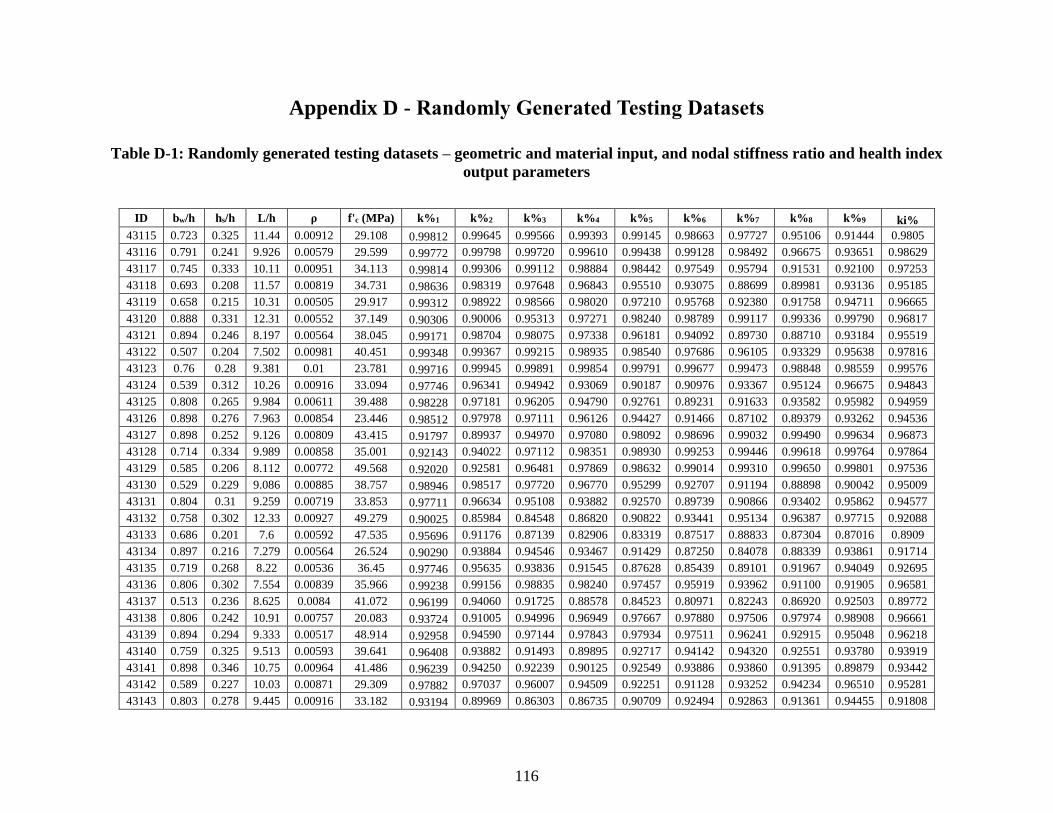
116

Appendix D - Randomly Generated Testing Datasets

Table D-1: Randomly generated testing datasets – geometric and material input, and nodal stiffness ratio and health index

output parameters

ID bw/h hs/h L/h ρ f'c (MPa) k%1 k%2 k%3 k%4 k%5 k%6 k%7 k%8 k%9 ki%

43115 0.723 0.325 11.44 0.00912 29.108 0.99812 0.99645 0.99566 0.99393 0.99145 0.98663 0.97727 0.95106 0.91444 0.9805

43116 0.791 0.241 9.926 0.00579 29.599 0.99772 0.99798 0.99720 0.99610 0.99438 0.99128 0.98492 0.96675 0.93651 0.98629

43117 0.745 0.333 10.11 0.00951 34.113 0.99814 0.99306 0.99112 0.98884 0.98442 0.97549 0.95794 0.91531 0.92100 0.97253

43118 0.693 0.208 11.57 0.00819 34.731 0.98636 0.98319 0.97648 0.96843 0.95510 0.93075 0.88699 0.89981 0.93136 0.95185

43119 0.658 0.215 10.31 0.00505 29.917 0.99312 0.98922 0.98566 0.98020 0.97210 0.95768 0.92380 0.91758 0.94711 0.96665

43120 0.888 0.331 12.31 0.00552 37.149 0.90306 0.90006 0.95313 0.97271 0.98240 0.98789 0.99117 0.99336 0.99790 0.96817

43121 0.894 0.246 8.197 0.00564 38.045 0.99171 0.98704 0.98075 0.97338 0.96181 0.94092 0.89730 0.88710 0.93184 0.95519

43122 0.507 0.204 7.502 0.00981 40.451 0.99348 0.99367 0.99215 0.98935 0.98540 0.97686 0.96105 0.93329 0.95638 0.97816

43123 0.76 0.28 9.381 0.01 23.781 0.99716 0.99945 0.99891 0.99854 0.99791 0.99677 0.99473 0.98848 0.98559 0.99576

43124 0.539 0.312 10.26 0.00916 33.094 0.97746 0.96341 0.94942 0.93069 0.90187 0.90976 0.93367 0.95124 0.96675 0.94843

43125 0.808 0.265 9.984 0.00611 39.488 0.98228 0.97181 0.96205 0.94790 0.92761 0.89231 0.91633 0.93582 0.95982 0.94959

43126 0.898 0.276 7.963 0.00854 23.446 0.98512 0.97978 0.97111 0.96126 0.94427 0.91466 0.87102 0.89379 0.93262 0.94536

43127 0.898 0.252 9.126 0.00809 43.415 0.91797 0.89937 0.94970 0.97080 0.98092 0.98696 0.99032 0.99490 0.99634 0.96873

43128 0.714 0.334 9.989 0.00858 35.001 0.92143 0.94022 0.97112 0.98351 0.98930 0.99253 0.99446 0.99618 0.99764 0.97864

43129 0.585 0.206 8.112 0.00772 49.568 0.92020 0.92581 0.96481 0.97869 0.98632 0.99014 0.99310 0.99650 0.99801 0.97536

43130 0.529 0.229 9.086 0.00885 38.757 0.98946 0.98517 0.97720 0.96770 0.95299 0.92707 0.91194 0.88898 0.90042 0.95009

43131 0.804 0.31 9.259 0.00719 33.853 0.97711 0.96634 0.95108 0.93882 0.92570 0.89739 0.90866 0.93402 0.95862 0.94577

43132 0.758 0.302 12.33 0.00927 49.279 0.90025 0.85984 0.84548 0.86820 0.90822 0.93441 0.95134 0.96387 0.97715 0.92088

43133 0.686 0.201 7.6 0.00592 47.535 0.95696 0.91176 0.87139 0.82906 0.83319 0.87517 0.88833 0.87304 0.87016 0.8909

43134 0.897 0.216 7.279 0.00564 26.524 0.90290 0.93884 0.94546 0.93467 0.91429 0.87250 0.84078 0.88339 0.93861 0.91714

43135 0.719 0.268 8.22 0.00536 36.45 0.97746 0.95635 0.93836 0.91545 0.87628 0.85439 0.89101 0.91967 0.94049 0.92695

43136 0.806 0.302 7.554 0.00839 35.966 0.99238 0.99156 0.98835 0.98240 0.97457 0.95919 0.93962 0.91100 0.91905 0.96581

43137 0.513 0.236 8.625 0.0084 41.072 0.96199 0.94060 0.91725 0.88578 0.84523 0.80971 0.82243 0.86920 0.92503 0.89772

43138 0.806 0.242 10.91 0.00757 20.083 0.93724 0.91005 0.94996 0.96949 0.97667 0.97880 0.97506 0.97974 0.98908 0.96661

43139 0.894 0.294 9.333 0.00517 48.914 0.92958 0.94590 0.97144 0.97843 0.97934 0.97511 0.96241 0.92915 0.95048 0.96218

43140 0.759 0.325 9.513 0.00593 39.641 0.96408 0.93882 0.91493 0.89895 0.92717 0.94142 0.94320 0.92551 0.93780 0.93919

43141 0.898 0.346 10.75 0.00964 41.486 0.96239 0.94250 0.92239 0.90125 0.92549 0.93886 0.93860 0.91395 0.89879 0.93442

43142 0.589 0.227 10.03 0.00871 29.309 0.97882 0.97037 0.96007 0.94509 0.92251 0.91128 0.93252 0.94234 0.96510 0.95281

43143 0.803 0.278 9.445 0.00916 33.182 0.93194 0.89969 0.86303 0.86735 0.90709 0.92494 0.92863 0.91361 0.94455 0.91808

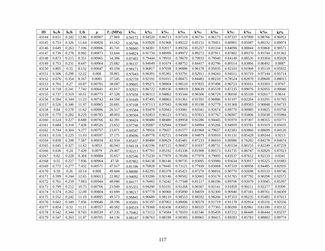
117

ID bw/h hs/h L/h ρ f'c (MPa) k%1 k%2 k%3 k%4 k%5 k%6 k%7 k%8 k%9 ki%

43144 0.651 0.242 12.86 0.00907 27.869 0.94172 0.94520 0.96713 0.97119 0.96731 0.96175 0.97337 0.97999 0.98766 0.96953

43145 0.753 0.326 11.64 0.00826 43.162 0.95796 0.93928 0.91968 0.89222 0.85151 0.79451 0.80901 0.85087 0.89232 0.89074

43146 0.649 0.263 7.106 0.00806 45.741 0.96660 0.94381 0.92017 0.89256 0.85257 0.81334 0.84096 0.88844 0.93868 0.90571

43147 0.739 0.278 8.992 0.00873 33.644 0.94824 0.91734 0.88999 0.89972 0.89272 0.87911 0.87802 0.89370 0.93744 0.91363

43148 0.873 0.215 8.351 0.00965 34.386 0.87403 0.79444 0.78910 0.78670 0.79933 0.79940 0.84149 0.88526 0.93304 0.85028

43149 0.753 0.231 8.647 0.00964 25.082 0.96137 0.94049 0.91674 0.88752 0.84417 0.82796 0.80514 0.83866 0.86492 0.8887

43150 0.805 0.35 8.132 0.00647 45.194 0.98171 0.96817 0.97038 0.96886 0.96178 0.95035 0.92103 0.91968 0.95119 0.95932

43151 0.506 0.298 12.22 0.008 39.801 0.97043 0.96391 0.95381 0.93791 0.92911 0.94243 0.94511 0.95719 0.97144 0.95714

43152 0.676 0.354 8.167 0.0081 37.545 0.92759 0.92191 0.91015 0.88475 0.84483 0.80210 0.78524 0.82870 0.89608 0.88013

43153 0.701 0.27 10.87 0.00791 38.047 0.99605 0.99271 0.98904 0.98510 0.97835 0.97498 0.96723 0.95051 0.93303 0.9767

43154 0.718 0.241 7.742 0.00641 41.017 0.92021 0.86722 0.89156 0.90019 0.88639 0.85539 0.87235 0.89076 0.92055 0.90046

43155 0.737 0.319 10.51 0.00773 47.528 0.97656 0.96312 0.94862 0.95344 0.96506 0.96729 0.96030 0.95339 0.92617 0.9614

43156 0.594 0.344 11.23 0.00742 44.184 0.91649 0.87495 0.88863 0.91361 0.91591 0.90086 0.91107 0.92204 0.93291 0.91765

43157 0.526 0.346 11.97 0.00865 20.681 0.97108 0.97113 0.97043 0.96368 0.95198 0.92779 0.91368 0.89503 0.90848 0.94733

43158 0.84 0.278 11.62 0.00896 26.517 0.95584 0.93479 0.93943 0.93981 0.93341 0.92674 0.89770 0.90985 0.93825 0.93758

43159 0.779 0.282 8.219 0.00785 48.003 0.90504 0.92453 0.96123 0.97431 0.97815 0.97767 0.96907 0.95806 0.95038 0.95984

43160 0.524 0.227 8.688 0.00766 42.391 0.90424 0.90480 0.88480 0.89958 0.92286 0.94445 0.95970 0.97307 0.98355 0.93771

43161 0.684 0.318 7.428 0.00526 23.652 0.97748 0.95087 0.92944 0.93647 0.94994 0.95266 0.94959 0.93781 0.91919 0.95035

43162 0.744 0.304 9.277 0.00757 23.071 0.84547 0.78916 0.79657 0.81577 0.81968 0.79657 0.82383 0.83860 0.88699 0.84126

43163 0.516 0.225 11.03 0.00597 37.171 0.89696 0.89778 0.92721 0.94508 0.94879 0.93910 0.91131 0.85428 0.89244 0.9213

43164 0.839 0.208 7.587 0.00818 42.934 0.85437 0.80480 0.80629 0.85481 0.87233 0.86010 0.80986 0.76202 0.84278 0.84674

43165 0.645 0.327 11.62 0.0053 46.943 0.84118 0.82196 0.87115 0.90457 0.91037 0.89731 0.85534 0.80155 0.82249 0.87259

43166 0.636 0.24 7.439 0.0079 29.407 0.92211 0.87701 0.85192 0.81336 0.81908 0.80573 0.81735 0.86747 0.92829 0.87023

43167 0.82 0.228 9.304 0.00884 35.657 0.82546 0.75230 0.77870 0.78186 0.77978 0.79005 0.83537 0.87612 0.92133 0.8341

43168 0.55 0.227 7.936 0.00964 47.58 0.87862 0.84138 0.86146 0.90735 0.93095 0.93980 0.93634 0.93917 0.95325 0.91883

43169 0.772 0.277 7.432 0.00571 47.017 0.81186 0.70828 0.70445 0.73121 0.77939 0.83068 0.87319 0.90958 0.94485 0.82935

43170 0.59 0.26 10.14 0.008 49.604 0.88080 0.82295 0.85378 0.85421 0.87270 0.90016 0.90770 0.92698 0.95533 0.89746

43171 0.599 0.244 12.65 0.00613 22.862 0.94092 0.93286 0.92146 0.90502 0.92665 0.93170 0.91765 0.87792 0.90298 0.92572

43172 0.761 0.259 7.003 0.00944 48.086 0.84177 0.76065 0.74242 0.77348 0.81117 0.86196 0.89706 0.92079 0.93045 0.85397

43173 0.799 0.212 10.75 0.00706 23.949 0.95355 0.94290 0.93191 0.91268 0.90307 0.92141 0.91859 0.90211 0.92277 0.9309

43174 0.574 0.262 12.08 0.00804 41.699 0.98217 0.97778 0.96969 0.95890 0.94059 0.92300 0.90940 0.87181 0.89761 0.94309

43175 0.552 0.242 11.19 0.00895 49.573 0.96845 0.96689 0.98110 0.98553 0.98592 0.98266 0.97353 0.96235 0.95485 0.97613

43176 0.602 0.349 7.056 0.00646 28.196 0.95691 0.91197 0.87962 0.89006 0.90579 0.91719 0.91178 0.92914 0.95316 0.92556

43177 0.854 0.32 11.11 0.00557 40.582 0.84519 0.79368 0.82436 0.83053 0.80335 0.77365 0.80200 0.82861 0.81180 0.83132

43178 0.542 0.344 8.743 0.00539 47.235 0.79462 0.73112 0.74584 0.78103 0.81546 0.85459 0.87212 0.86449 0.86444 0.83237

43179 0.547 0.263 11.97 0.00705 44.136 0.88147 0.86763 0.88199 0.90385 0.89965 0.90415 0.89283 0.85783 0.88802 0.89774

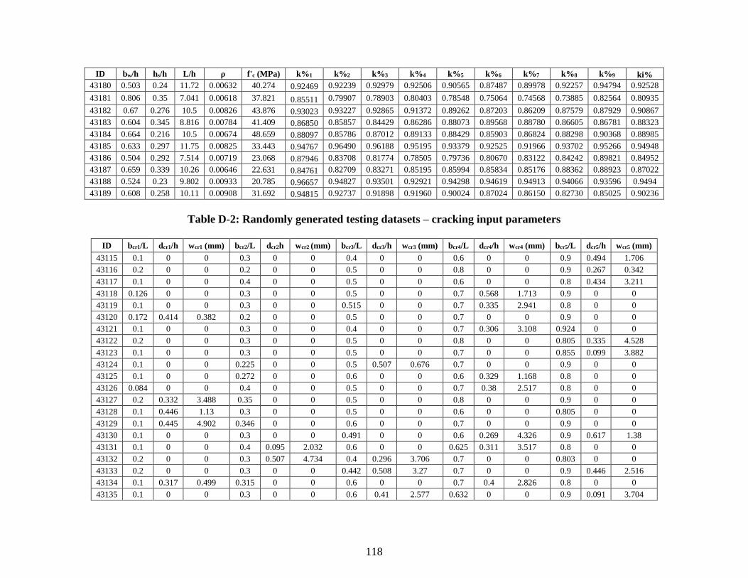
118

ID bw/h hs/h L/h ρ f'c (MPa) k%1 k%2 k%3 k%4 k%5 k%6 k%7 k%8 k%9 ki%

43180 0.503 0.24 11.72 0.00632 40.274 0.92469 0.92239 0.92979 0.92506 0.90565 0.87487 0.89978 0.92257 0.94794 0.92528

43181 0.806 0.35 7.041 0.00618 37.821 0.85511 0.79907 0.78903 0.80403 0.78548 0.75064 0.74568 0.73885 0.82564 0.80935

43182 0.67 0.276 10.5 0.00826 43.876 0.93023 0.93227 0.92865 0.91372 0.89262 0.87203 0.86209 0.87579 0.87929 0.90867

43183 0.604 0.345 8.816 0.00784 41.409 0.86850 0.85857 0.84429 0.86286 0.88073 0.89568 0.88780 0.86605 0.86781 0.88323

43184 0.664 0.216 10.5 0.00674 48.659 0.88097 0.85786 0.87012 0.89133 0.88429 0.85903 0.86824 0.88298 0.90368 0.88985

43185 0.633 0.297 11.75 0.00825 33.443 0.94767 0.96490 0.96188 0.95195 0.93379 0.92525 0.91966 0.93702 0.95266 0.94948

43186 0.504 0.292 7.514 0.00719 23.068 0.87946 0.83708 0.81774 0.78505 0.79736 0.80670 0.83122 0.84242 0.89821 0.84952

43187 0.659 0.339 10.26 0.00646 22.631 0.84761 0.82709 0.83271 0.85195 0.85994 0.85834 0.85176 0.88362 0.88923 0.87022

43188 0.524 0.23 9.802 0.00933 20.785 0.96657 0.94827 0.93501 0.92921 0.94298 0.94619 0.94913 0.94066 0.93596 0.9494

43189 0.608 0.258 10.11 0.00908 31.692 0.94815 0.92737 0.91898 0.91960 0.90024 0.87024 0.86150 0.82730 0.85025 0.90236

Table D-2: Randomly generated testing datasets – cracking input parameters

ID bcr1/L dcr1/h wcr1 (mm) bcr2/L dcr2h wcr2 (mm) bcr3/L dcr3/h wcr3 (mm) bcr4/L dcr4/h wcr4 (mm) bcr5/L dcr5/h wcr5 (mm)

43115 0.1 0 0 0.3 0 0 0.4 0 0 0.6 0 0 0.9 0.494 1.706

43116 0.2 0 0 0.2 0 0 0.5 0 0 0.8 0 0 0.9 0.267 0.342

43117 0.1 0 0 0.4 0 0 0.5 0 0 0.6 0 0 0.8 0.434 3.211

43118 0.126 0 0 0.3 0 0 0.5 0 0 0.7 0.568 1.713 0.9 0 0

43119 0.1 0 0 0.3 0 0 0.515 0 0 0.7 0.335 2.941 0.8 0 0

43120 0.172 0.414 0.382 0.2 0 0 0.5 0 0 0.7 0 0 0.9 0 0

43121 0.1 0 0 0.3 0 0 0.4 0 0 0.7 0.306 3.108 0.924 0 0

43122 0.2 0 0 0.3 0 0 0.5 0 0 0.8 0 0 0.805 0.335 4.528

43123 0.1 0 0 0.3 0 0 0.5 0 0 0.7 0 0 0.855 0.099 3.882

43124 0.1 0 0 0.225 0 0 0.5 0.507 0.676 0.7 0 0 0.9 0 0

43125 0.1 0 0 0.272 0 0 0.6 0 0 0.6 0.329 1.168 0.8 0 0

43126 0.084 0 0 0.4 0 0 0.5 0 0 0.7 0.38 2.517 0.8 0 0

43127 0.2 0.332 3.488 0.35 0 0 0.5 0 0 0.8 0 0 0.9 0 0

43128 0.1 0.446 1.13 0.3 0 0 0.5 0 0 0.6 0 0 0.805 0 0

43129 0.1 0.445 4.902 0.346 0 0 0.6 0 0 0.7 0 0 0.9 0 0

43130 0.1 0 0 0.3 0 0 0.491 0 0 0.6 0.269 4.326 0.9 0.617 1.38

43131 0.1 0 0 0.4 0.095 2.032 0.6 0 0 0.625 0.311 3.517 0.8 0 0

43132 0.2 0 0 0.3 0.507 4.734 0.4 0.296 3.706 0.7 0 0 0.803 0 0

43133 0.2 0 0 0.3 0 0 0.442 0.508 3.27 0.7 0 0 0.9 0.446 2.516

43134 0.1 0.317 0.499 0.315 0 0 0.6 0 0 0.7 0.4 2.826 0.8 0 0

43135 0.1 0 0 0.3 0 0 0.6 0.41 2.577 0.632 0 0 0.9 0.091 3.704

119

ID bcr1/L dcr1/h wcr1 (mm) bcr2/L dcr2h wcr2 (mm) bcr3/L dcr3/h wcr3 (mm) bcr4/L dcr4/h wcr4 (mm) bcr5/L dcr5/h wcr5 (mm)

43136 0.2 0 0 0.239 0 0 0.6 0 0 0.7 0.104 0.044 0.8 0.356 2.023

43137 0.1 0 0 0.4 0 0 0.566 0.572 2.53 0.7 0.433 4.621 0.8 0 0

43138 0.1 0 0 0.206 0.359 0.979 0.6 0 0 0.7 0.095 4.276 0.8 0 0

43139 0.1 0.216 1.625 0.4 0 0 0.5 0 0 0.7 0 0 0.808 0.187 3.879

43140 0.1 0 0 0.4 0.306 1.177 0.5 0 0 0.8 0 0 0.829 0.224 0.435

43141 0.1 0 0 0.3 0 0 0.4 0.298 4.033 0.748 0 0 0.9 0.35 1.127

43142 0.1 0 0 0.2 0 0 0.563 0.437 1.01 0.8 0.087 3.339 0.9 0 0

43143 0.11 0 0 0.4 0.543 4.789 0.4 0 0 0.6 0 0 0.8 0.206 2.157

43144 0.16 0.359 1.616 0.4 0 0 0.6 0.176 3.621 0.6 0 0 0.9 0 0

43145 0.1 0 0 0.2 0 0 0.6 0.5 1.3 0.644 0.565 3.206 0.8 0.029 0.543

43146 0.077 0 0 0.341 0.043 1.464 0.507 0.099 4.494 0.615 0.574 4.407 0.899 0 0

43147 0.1 0 0 0.3 0.26 3.476 0.6 0.256 4.201 0.734 0.284 0.199 0.8 0 0

43148 0.1 0 0 0.2 0.507 0.106 0.4 0.363 0.253 0.6 0.429 0.382 0.9 0 0

43149 0.2 0 0 0.2 0 0 0.5 0.467 4.144 0.7 0.626 2.912 0.918 0.304 1.41

43150 0.1 0 0 0.2 0.09 3.608 0.5 0.046 4.223 0.739 0.249 0.187 0.9 0 0

43151 0.1 0.072 1.923 0.222 0 0 0.5 0.353 4.422 0.7 0.16 1.975 0.8 0 0

43152 0.1 0.196 0.562 0.4 0 0 0.574 0.398 4.491 0.7 0.602 3.304 0.9 0 0

43153 0.1 0 0 0.3 0 0 0.5 0.078 4.449 0.773 0.132 3.974 0.9 0.299 0.655

43154 0.1 0 0 0.2 0.349 4.955 0.55 0 0 0.6 0.354 3.214 0.9 0.166 3.94

43155 0.1 0 0 0.3 0.173 2.096 0.409 0 0 0.7 0.102 2.114 0.9 0.301 2.286

43156 0.1 0 0 0.243 0.543 0.147 0.6 0 0 0.6 0.358 2.238 0.9 0.182 4.034

43157 0.1 0.14 2.639 0.353 0 0 0.4 0 0 0.6 0.397 1.616 0.8 0.568 3.039

43158 0.1 0 0 0.2 0.168 2.895 0.5 0.121 3.223 0.7 0.4 3.661 0.912 0 0

43159 0.133 0.404 1.267 0.2 0 0 0.5 0 0 0.8 0.104 3.352 0.9 0.148 1.383

43160 0.1 0.44 1.92 0.3 0.427 1.035 0.5 0.093 2.133 0.65 0.014 3.794 0.8 0 0

43161 0.2 0 0 0.3 0.192 3.219 0.6 0.062 3.754 0.8 0.084 0.079 0.893 0.28 3.562

43162 0.2 0.56 1.337 0.3 0.42 3.354 0.549 0 0 0.6 0.627 3.643 0.8 0.241 4.823

43163 0.081 0.387 4.748 0.2 0.384 1.322 0.6 0 0 0.8 0.165 2.571 0.8 0.567 3.291

43164 0.134 0.196 4.038 0.3 0.535 4.232 0.6 0 0 0.7 0.232 4.02 0.8 0.615 1.682

43165 0.2 0.419 2.71 0.2 0.417 0.067 0.4 0 0 0.8 0.464 2.486 0.845 0.498 1.818

43166 0.1 0.2 2.613 0.262 0 0 0.4 0.469 3.404 0.7 0.621 0.59 0.9 0.007 0.212

43167 0.2 0.185 1.684 0.2 0.633 4.81 0.5 0.46 0.303 0.6 0.405 2.299 0.885 0 0

43168 0.1 0.537 0.346 0.3 0.484 0.907 0.4 0 0 0.7 0.121 3.051 0.857 0.182 1.889

43169 0.186 0.203 1.965 0.3 0.615 3.013 0.4 0.461 2.84 0.6 0.09 1.272 0.8 0 0

43170 0.199 0 0 0.2 0.627 2.406 0.4 0.41 2.566 0.7 0.165 3.625 0.8 0.012 4.788

43171 0.1 0.131 3.223 0.4 0.391 3.207 0.5 0 0 0.8 0.535 2.785 0.88 0.108 0.163

120

ID bcr1/L dcr1/h wcr1 (mm) bcr2/L dcr2h wcr2 (mm) bcr3/L dcr3/h wcr3 (mm) bcr4/L dcr4/h wcr4 (mm) bcr5/L dcr5/h wcr5 (mm)

43172 0.2 0.364 4.816 0.3 0.635 0.247 0.5 0.345 2.985 0.6 0 0 0.912 0.139 0.469

43173 0.1 0.106 0.354 0.3 0 0 0.5 0.335 1.614 0.751 0.129 2.937 0.8 0.207 1.847

43174 0.1 0.033 1.333 0.4 0 0 0.5 0.136 4.734 0.638 0.175 0.795 0.8 0.575 3.258

43175 0.2 0.18 4.674 0.2 0.055 4.924 0.5 0.003 4.063 0.7 0.111 3.152 0.873 0.204 4.204

43176 0.2 0.031 4.148 0.323 0.351 2.364 0.5 0.105 1.623 0.7 0.21 2.003 0.9 0.076 0.049

43177 0.2 0.387 3.781 0.3 0.197 2.52 0.6 0.397 1.225 0.6 0.375 3.021 0.918 0.494 1.905

43178 0.2 0.618 4.526 0.3 0.571 1.657 0.4 0.407 4.9 0.7 0.019 0.806 0.869 0.511 4.52

43179 0.1 0.454 2.664 0.2 0.501 0.623 0.523 0.239 3.826 0.8 0.331 2.958 0.8 0.37 0.243

43180 0.1 0.349 1.64 0.2 0.217 2.548 0.5 0.027 0.343 0.601 0.565 0.053 0.8 0.048 1.516

43181 0.1 0.231 1.545 0.277 0.359 3.194 0.6 0.377 4.983 0.7 0.187 2.534 0.8 0.536 1.461

43182 0.1 0.199 4.177 0.252 0.05 4.026 0.5 0.174 0.057 0.7 0.467 1.444 0.9 0.336 4.502

43183 0.081 0.47 0.463 0.286 0.406 4.072 0.444 0.249 4.086 0.762 0.272 0.578 0.885 0.471 2.723

43184 0.1 0.184 4.241 0.2 0.427 4.619 0.593 0.35 0.347 0.7 0.155 3.092 0.9 0.203 3.066

43185 0.085 0.272 2.656 0.4 0.026 0.967 0.5 0.175 2.974 0.7 0.294 2.573 0.9 0.073 0.601

43186 0.1 0.529 2.543 0.4 0.561 3.98 0.5 0.245 0.33 0.6 0.351 2.381 0.8 0.451 3.863

43187 0.149 0.596 2.277 0.3 0.397 3.82 0.5 0.162 2.08 0.7 0.449 1.95 0.9 0.397 3.961

43188 0.2 0.087 3.645 0.305 0.107 4.223 0.4 0.272 2.035 0.6 0.098 3.531 0.9 0.403 0.777

43189 0.1 0.077 2.878 0.3 0.213 0.052 0.594 0.388 0.712 0.8 0.567 1.066 0.9 0.36 1.366