Embed Size (px)
Citation preview
FE-FatigueRELEASE 5.0
Worked Examplesusing
Studio FE Display

Copyright Notice
All of this documentation, and the software it describes, are copyrighted with all rights reserved. Under copyright laws; Neither the documentation or the software may be copied, photocopied, or reproduced in any way, translated, or converted into any machine readable form or any electronic medium, in whole or in part, without express written permission from nCode International Ltd. (nCode). Failure to obtain such permission may result in prosecution.
The software suite that comprises nSoft V5.3 (the product) and FE-Fatigue and its component programs and files, are the property of nCode. nSoft V5.3 and FE-Fatigue are protected under copyright law and are licensed for use only by a user who has obtained the necessary license, or in the case of a multi user licence may only be used by up to the maximum number of users specified in the licence agreement. The sale, lease, hire rental, or any other reassignment of the product to, or by, a third party without the prior written consent of nCode is expressly forbidden.
All Worldwide Rights Reserved, 1999, 2000,2001,2002.
nSoft documents are viewed using Adobe Acrobat Reader.“Acrobat® Reader Copyright © 1987-1996 Adobe Systems Incorporated. All rights reserved. Adobe and Acrobat are trademarks of Adobe Systems Incorporated which may be registered in certain jurisdictions.”
All other trademarks are the property of their respective owners.
Warranty Notice
Whilst nCode makes the product as reliable as is reasonably possible, nCode does not warrant that the product will function properly under all hardware platforms or software environments. Certain combinations of third party software and/or manufacturers modifications to hardware and software may impact upon the operation of nCode software.
nCode has tested the software and reviewed the documentation but nCode MAKES NO WARRANTY, IMPLICIT OR EXPLICIT, WITH RESPECT TO THE PRODUCT, TO ITS QUALITY, PERFORMANCE, MERCHANTABILITY, OR FITNESS FOR A SPECIFIC USAGE. THIS SOFTWARE AND DOCUMENTATION ARE LICENSED ‘AS IS’ AND YOU - THE LICENSEE - ASSUME THE ENTIRE RISK AS TO THEIR QUALITY AND PERFORMANCE, WHEN YOU USE THE PRODUCT.
Liability Notice
NCODE WILL NOT BE LIABLE FOR DAMAGES ARISING FROM THE RESULTS, DIRECT OR INDIRECT, SPECIAL, INCIDENTAL, OR CONSEQUENTIAL, OF THE LICENCEES USAGE OR MISUSAGE OF THE PRODUCT, even if advised of the possibility of such damages. In particular, and without prejudice to the foregoing, nCode has no liability for any programs or data stored or used with nCode software, including the costs of recovering such programs or data.
nCode International Ltd.230 Woodbourne RoadSheffieldS9 3LQEngland

Introduction . . . . . . . . . . . . . . . . . . . . . . . . . . . . . . . . . . . 6
1. Simple E-N example – Bracket analysis . . . . . . . . . . 7
2. Simple S-N Example – Bracket analysis . . . . . . . . . . 27
3. Multiple Loads Example . . . . . . . . . . . . . . . . . . . . . . . 39
4. Spot Weld Analysis example . . . . . . . . . . . . . . . . . . . 60
5. Multiaxial Strain-Life Example - SAE Notched Shaft 75

IntroductionThe following examples have been written to use the FE model and fatigue results postprocessing features of the FE Display plugin of Studio.
The examples make use of files available in the demo directory:
<installation path>\ncodev53\demo
In order to run these examples, you will need to have installed and licensed the Studio FE Display plugin.
FE-Fatigue Worked Examples using Studio Page 7
1. Simple E-N example – Bracket analysisIn this example, you will use the bracket model and perform a Strain-Life (E-N) analysis to calculate life to initiate a crack with a variable amplitude loading function.
The Strain-Life method relates the local strain to life to initiate an engineering crack (1-2mm). The S-N method uses the elastic stresses directly to calculate fatigue lives but the Strain-Life approach in FE-Fatigue takes elastic stresses or strains from FE analysis and estimates the actual elastic-plastic strain at each location.
This example uses nCode’s Studio FE Display to show the model and results and uses the FE2FES translator to read the stresses from an ANSYS bracket.rst file.
1.1 IntroductionThis example problem has a bracket bolted to a box section. A vertical load is applied to the end of the bracket. The example calculates how many times a variable amplitude load time history (bracket.dac) can be repeated before a crack will initiate. The example uses SAE standard fatigue properties for 1008 steel.
The following files are required for this example:
bracket.rstbracket.dac
It is suggested you copy these files to a new directory before beginning this exercise.
FE-Fatigue Worked Examples using Studio Page 8
1.2 Displaying the model in StudioTo view the model prior to starting the analysis, we will use the nSoft Studio module.
• Start the main nSoft interface, select Display from the nSoft Menu, and select Studio Display/Reporting Tool (studio)
Studio will start and show an empty display area. To insert the model on the display page:
• Select Insert > FE Display
• In the file selection form, select bracket.rst from the working directory and click on Open.
The model will be shown on the current Studio page. (Other displays can be added to the same page or a single view can be selected by using View > Interactive Mode.)
The model can be dynamically manipulated in the display by holding down either the Control or Shift keys together with the mouse buttons. (Alternatively, function F2 and F3 keys can be used). Put the cursor on the display and move mouse to manipulate the model. The controls are summarized as:
Rotate – CTRL+ Left Mouse Button, or F2 + Left Mouse Button
Pan – CTRL + Right Mouse Button, or F2 + Right Mouse Button
Cursor Zoom – SHIFT + Left Mouse Button, or F3 + Left Mouse Button
Box Zoom – SHIFT + Middle Mouse Button, or F3 + Middle Mouse Button
Squiggle Zoom - SHIFT + Right Mouse Button, or F3 + Right Mouse Button
NOTE: The Controls Summary is also available by clicking the mouse icon on the toolbar.
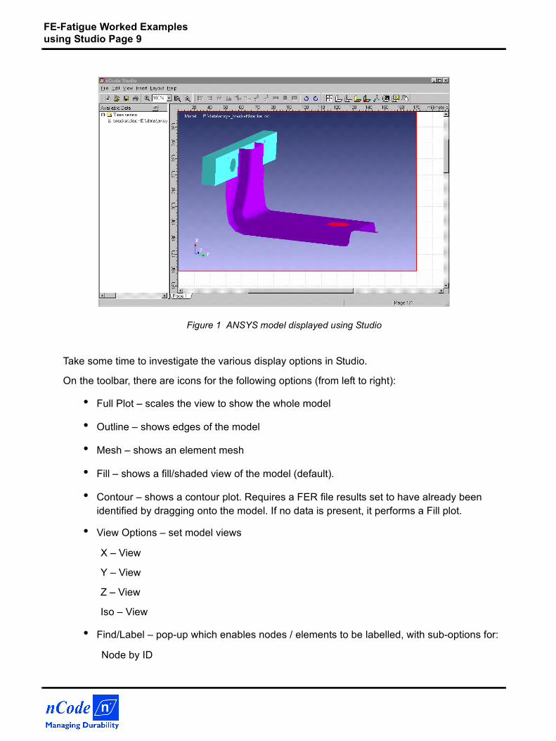
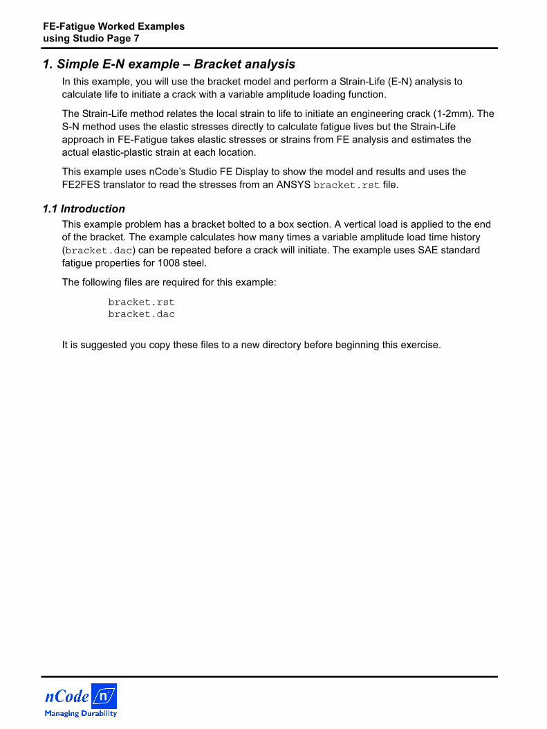
FE-Fatigue Worked Examples using Studio Page 9
Figure 1 ANSYS model displayed using Studio
Take some time to investigate the various display options in Studio.
On the toolbar, there are icons for the following options (from left to right):
• Full Plot – scales the view to show the whole model
• Outline – shows edges of the model
• Mesh – shows an element mesh
• Fill – shows a fill/shaded view of the model (default).
• Contour – shows a contour plot. Requires a FER file results set to have already been identified by dragging onto the model. If no data is present, it performs a Fill plot.
• View Options – set model views
X – View
Y – View
Z – View
Iso – View
• Find/Label – pop-up which enables nodes / elements to be labelled, with sub-options for:
Node by ID
FE-Fatigue Worked Examples using Studio Page 10
Element by ID
Clear labels
• Model Summary – a pop-up list containing:
Model file name
Number of Nodes
Number of Elements
Number of Elements divided by type i.e., solids, shells, bars, others
• Controls Summary – lists the dynamic model controls available via mouse buttons
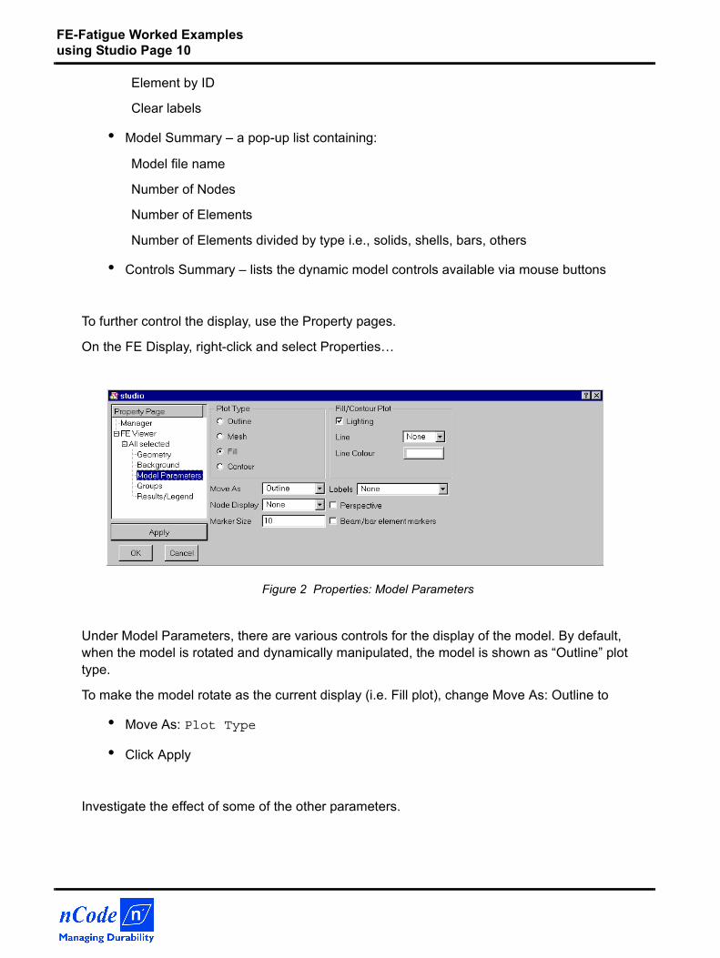
To further control the display, use the Property pages.
On the FE Display, right-click and select Properties…
Figure 2 Properties: Model Parameters
Under Model Parameters, there are various controls for the display of the model. By default, when the model is rotated and dynamically manipulated, the model is shown as “Outline” plot type.
To make the model rotate as the current display (i.e. Fill plot), change Move As: Outline to
• Move As: Plot Type
• Click Apply
Investigate the effect of some of the other parameters.
FE-Fatigue Worked Examples using Studio Page 11
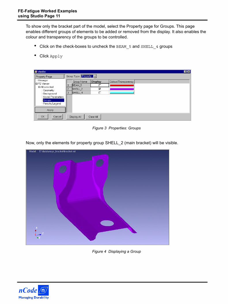
To show only the bracket part of the model, select the Property page for Groups. This page enables different groups of elements to be added or removed from the display. It also enables the colour and transparency of the groups to be controlled.
• Click on the check-boxes to uncheck the BEAM_5 and SHELL_4 groups
• Click Apply
Figure 3 Properties: Groups
Now, only the elements for property group SHELL_2 (main bracket) will be visible.
Figure 4 Displaying a Group
FE-Fatigue Worked Examples using Studio Page 12
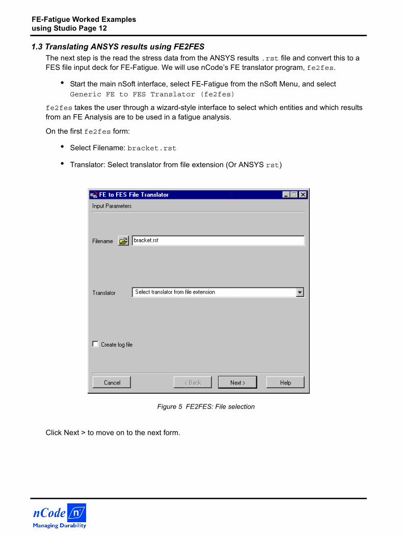
1.3 Translating ANSYS results using FE2FESThe next step is the read the stress data from the ANSYS results .rst file and convert this to a FES file input deck for FE-Fatigue. We will use nCode’s FE translator program, fe2fes.
• Start the main nSoft interface, select FE-Fatigue from the nSoft Menu, and select Generic FE to FES Translator (fe2fes)
fe2fes takes the user through a wizard-style interface to select which entities and which results from an FE Analysis are to be used in a fatigue analysis.
On the first fe2fes form:
• Select Filename: bracket.rst
• Translator: Select translator from file extension (Or ANSYS rst)
Figure 5 FE2FES: File selection
Click Next > to move on to the next form.
FE-Fatigue Worked Examples using Studio Page 13
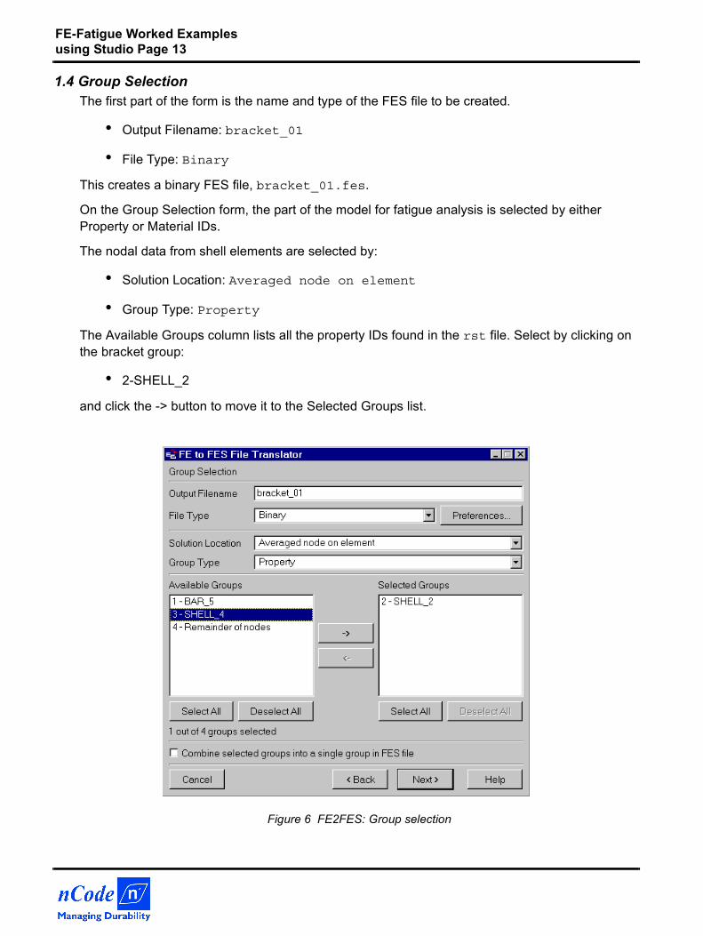
1.4 Group SelectionThe first part of the form is the name and type of the FES file to be created.
• Output Filename: bracket_01
• File Type: Binary
This creates a binary FES file, bracket_01.fes.
On the Group Selection form, the part of the model for fatigue analysis is selected by either Property or Material IDs.
The nodal data from shell elements are selected by:
• Solution Location: Averaged node on element
• Group Type: Property
The Available Groups column lists all the property IDs found in the rst file. Select by clicking on the bracket group:
• 2-SHELL_2
and click the -> button to move it to the Selected Groups list.
Figure 6 FE2FES: Group selection
FE-Fatigue Worked Examples using Studio Page 14
The “Combine selected groups into a single group in FES file” option can be checked if you wish to make it easier to use the same fatigue properties across a whole model.
Click the ungreyed Next > button to move on to the next form. (You can also back up at any stage using < Back.)
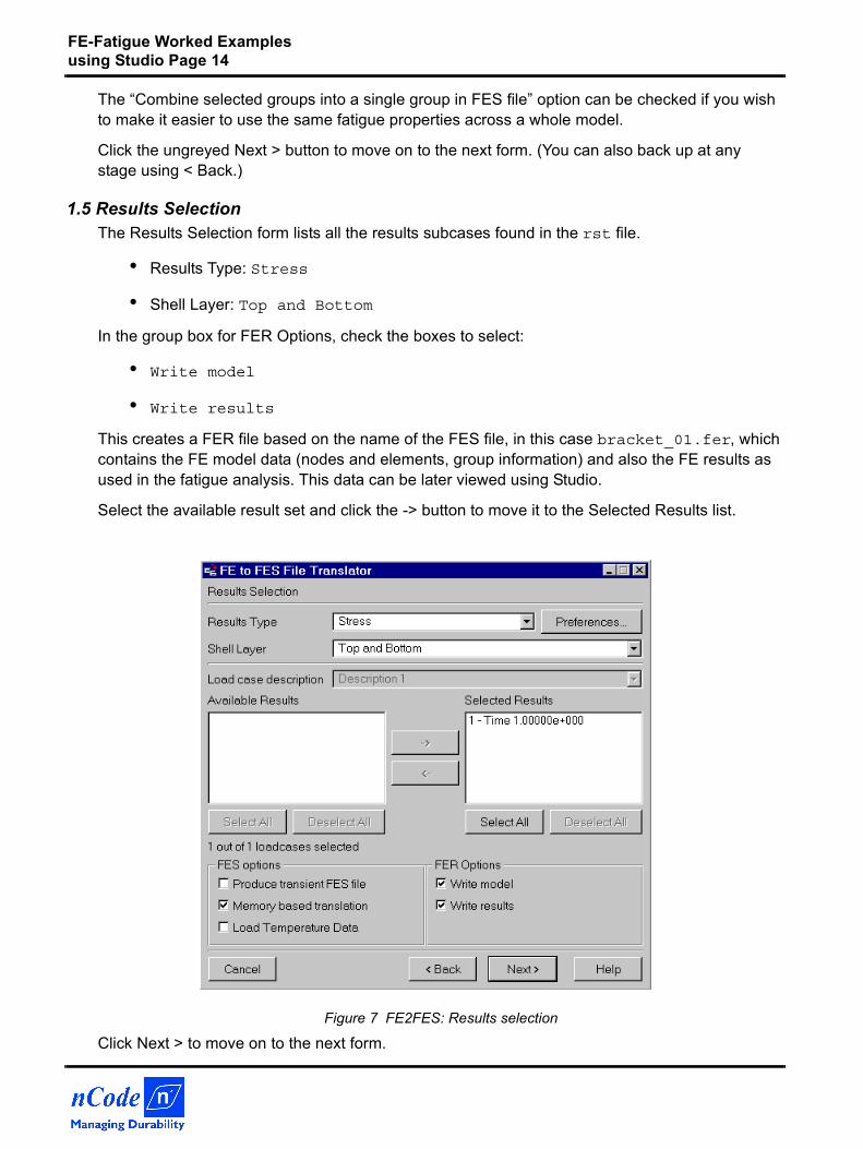
1.5 Results SelectionThe Results Selection form lists all the results subcases found in the rst file.
• Results Type: Stress
• Shell Layer: Top and Bottom
In the group box for FER Options, check the boxes to select:
• Write model
• Write results
This creates a FER file based on the name of the FES file, in this case bracket_01.fer, which contains the FE model data (nodes and elements, group information) and also the FE results as used in the fatigue analysis. This data can be later viewed using Studio.
Select the available result set and click the -> button to move it to the Selected Results list.
Figure 7 FE2FES: Results selection
Click Next > to move on to the next form.
FE-Fatigue Worked Examples using Studio Page 15
The final form is a summary of the translation.
Check the “Start FE-Fatigue with FES file” box and click on Finish and the fatfe FE-Fatigue solver program is shown. (Alternatively, you can start fatfe separately and select bracket_01.fes as the Input Fatigue Filename.)
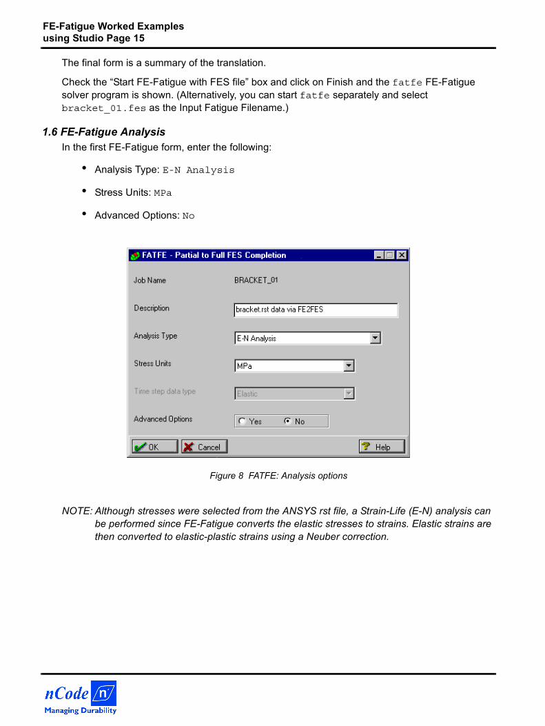
1.6 FE-Fatigue AnalysisIn the first FE-Fatigue form, enter the following:
• Analysis Type: E-N Analysis
• Stress Units: MPa
• Advanced Options: No
Figure 8 FATFE: Analysis options
NOTE: Although stresses were selected from the ANSYS rst file, a Strain-Life (E-N) analysis can be performed since FE-Fatigue converts the elastic stresses to strains. Elastic strains are then converted to elastic-plastic strains using a Neuber correction.
FE-Fatigue Worked Examples using Studio Page 16
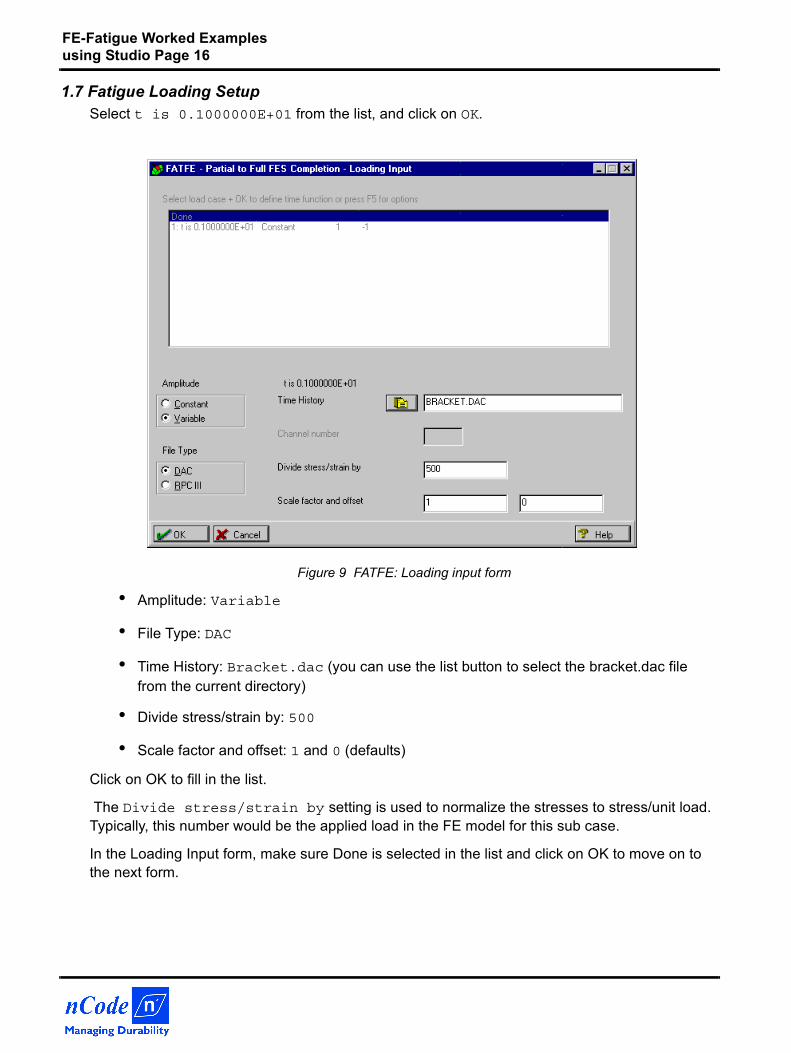
1.7 Fatigue Loading SetupSelect t is 0.1000000E+01 from the list, and click on OK.
Figure 9 FATFE: Loading input form
• Amplitude: Variable
• File Type: DAC
• Time History: Bracket.dac (you can use the list button to select the bracket.dac file from the current directory)
• Divide stress/strain by: 500
• Scale factor and offset: 1 and 0 (defaults)
Click on OK to fill in the list.
The Divide stress/strain by setting is used to normalize the stresses to stress/unit load. Typically, this number would be the applied load in the FE model for this sub case.
In the Loading Input form, make sure Done is selected in the list and click on OK to move on to the next form.
FE-Fatigue Worked Examples using Studio Page 17
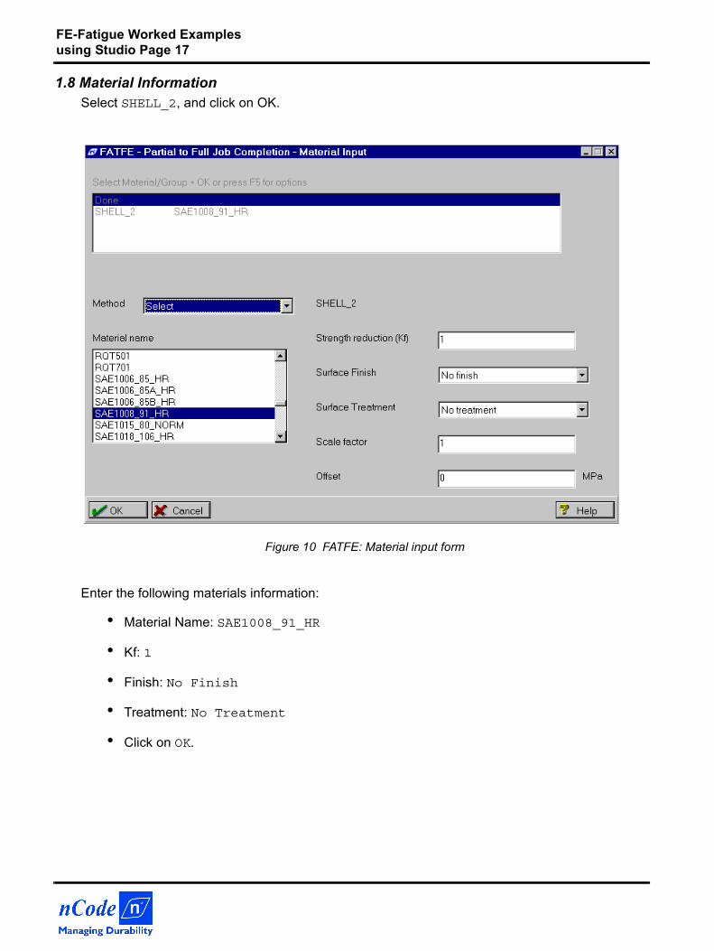
1.8 Material InformationSelect SHELL_2, and click on OK.
Figure 10 FATFE: Material input form
Enter the following materials information:
• Material Name: SAE1008_91_HR
• Kf: 1
• Finish: No Finish
• Treatment: No Treatment
• Click on OK.
FE-Fatigue Worked Examples using Studio Page 18
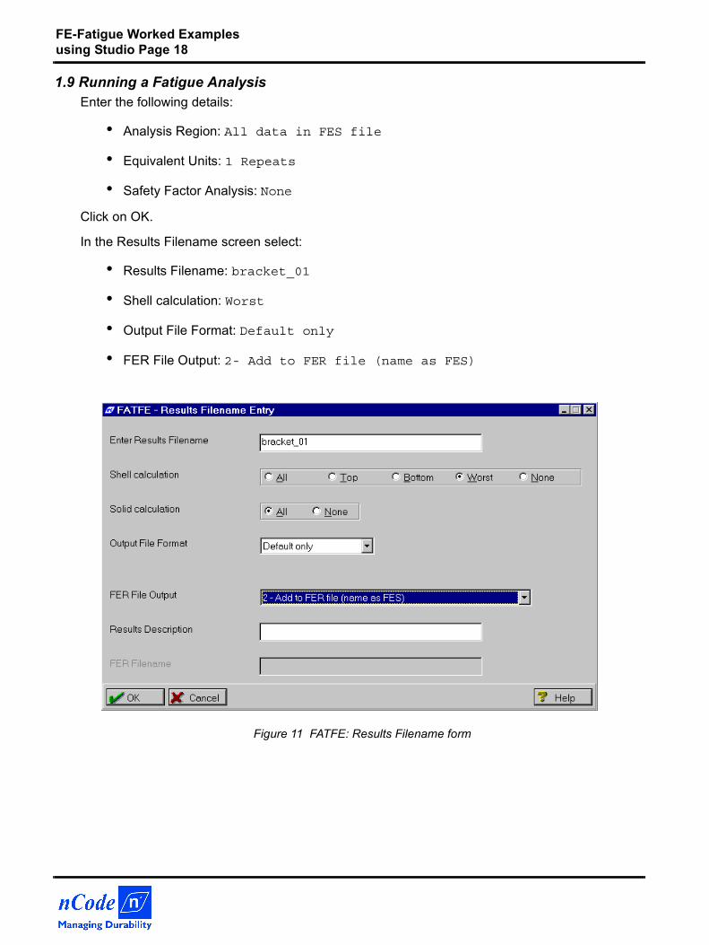
1.9 Running a Fatigue AnalysisEnter the following details:
• Analysis Region: All data in FES file
• Equivalent Units: 1 Repeats
• Safety Factor Analysis: None
Click on OK.
In the Results Filename screen select:
• Results Filename: bracket_01
• Shell calculation: Worst
• Output File Format: Default only
• FER File Output: 2- Add to FER file (name as FES)
Figure 11 FATFE: Results Filename form
FE-Fatigue Worked Examples using Studio Page 19
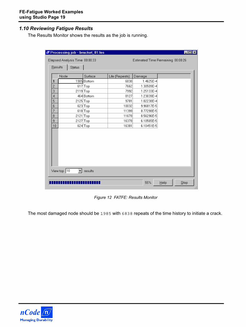
1.10 Reviewing Fatigue ResultsThe Results Monitor shows the results as the job is running.
Figure 12 FATFE: Results Monitor
The most damaged node should be 1985 with 6838 repeats of the time history to initiate a crack.
FE-Fatigue Worked Examples using Studio Page 20
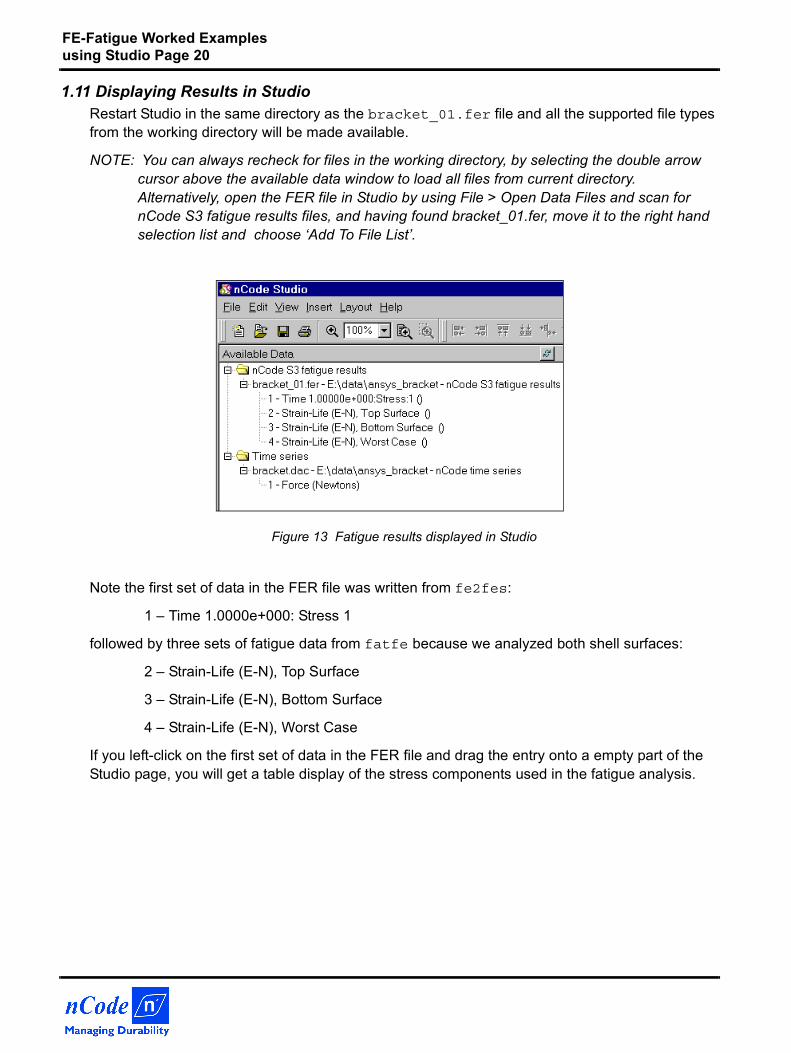
1.11 Displaying Results in StudioRestart Studio in the same directory as the bracket_01.fer file and all the supported file types from the working directory will be made available.
NOTE: You can always recheck for files in the working directory, by selecting the double arrow cursor above the available data window to load all files from current directory. Alternatively, open the FER file in Studio by using File > Open Data Files and scan for nCode S3 fatigue results files, and having found bracket_01.fer, move it to the right hand selection list and choose ‘Add To File List’.
Figure 13 Fatigue results displayed in Studio
Note the first set of data in the FER file was written from fe2fes:
1 – Time 1.0000e+000: Stress 1
followed by three sets of fatigue data from fatfe because we analyzed both shell surfaces:
2 – Strain-Life (E-N), Top Surface
3 – Strain-Life (E-N), Bottom Surface
4 – Strain-Life (E-N), Worst Case
If you left-click on the first set of data in the FER file and drag the entry onto a empty part of the Studio page, you will get a table display of the stress components used in the fatigue analysis.
FE-Fatigue Worked Examples using Studio Page 21
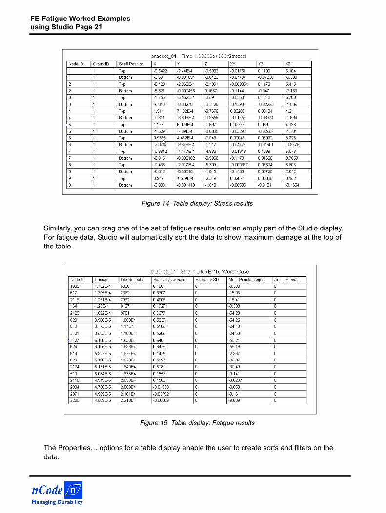
Figure 14 Table display: Stress results
Similarly, you can drag one of the set of fatigue results onto an empty part of the Studio display. For fatigue data, Studio will automatically sort the data to show maximum damage at the top of the table.
Figure 15 Table display: Fatigue results
The Properties… options for a table display enable the user to create sorts and filters on the data.
FE-Fatigue Worked Examples using Studio Page 22
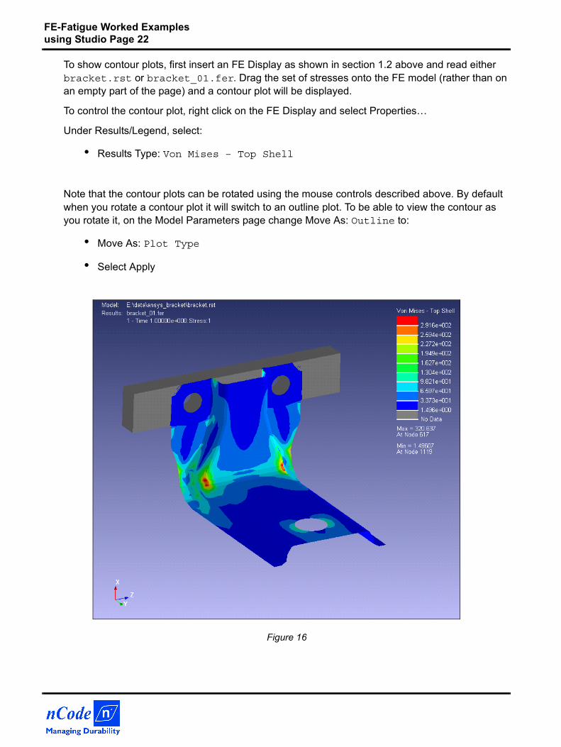
To show contour plots, first insert an FE Display as shown in section 1.2 above and read either bracket.rst or bracket_01.fer. Drag the set of stresses onto the FE model (rather than on an empty part of the page) and a contour plot will be displayed.
To control the contour plot, right click on the FE Display and select Properties…
Under Results/Legend, select:
• Results Type: Von Mises – Top Shell
Note that the contour plots can be rotated using the mouse controls described above. By default when you rotate a contour plot it will switch to an outline plot. To be able to view the contour as you rotate it, on the Model Parameters page change Move As: Outline to:
• Move As: Plot Type
• Select Apply
Figure 16
FE-Fatigue Worked Examples using Studio Page 23
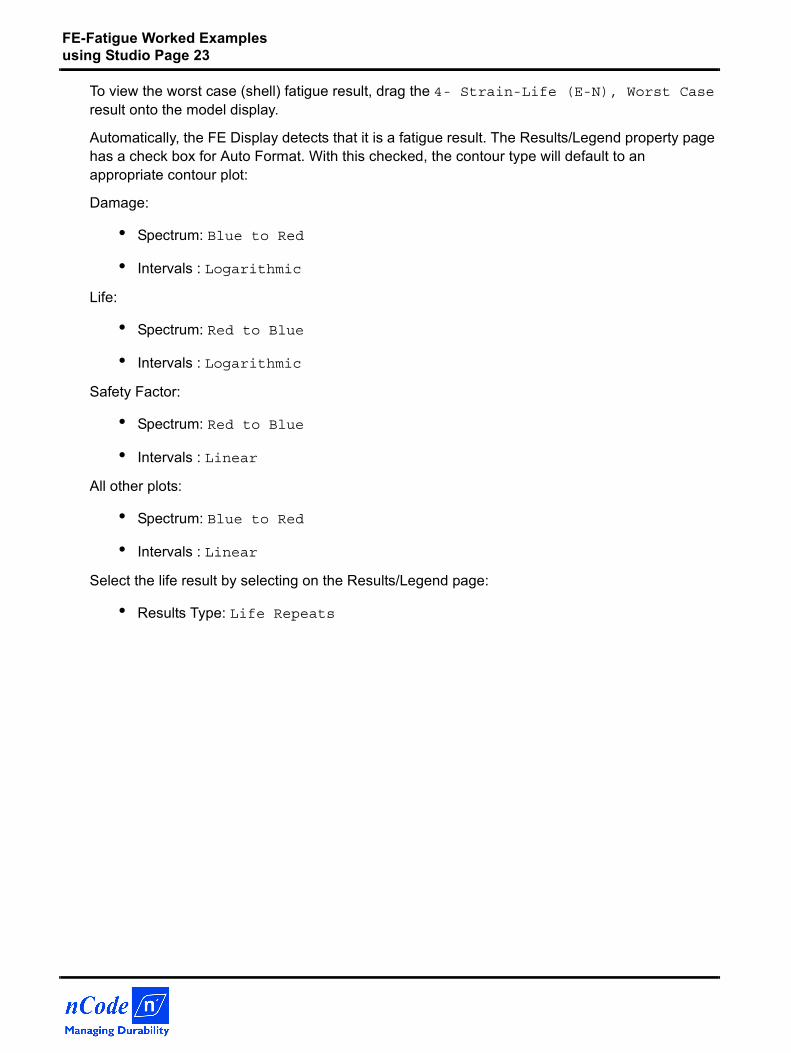
To view the worst case (shell) fatigue result, drag the 4- Strain-Life (E-N), Worst Case result onto the model display.
Automatically, the FE Display detects that it is a fatigue result. The Results/Legend property page has a check box for Auto Format. With this checked, the contour type will default to an appropriate contour plot:
Damage:
• Spectrum: Blue to Red
• Intervals : Logarithmic
Life:
• Spectrum: Red to Blue
• Intervals : Logarithmic
Safety Factor:
• Spectrum: Red to Blue
• Intervals : Linear
All other plots:
• Spectrum: Blue to Red
• Intervals : Linear
Select the life result by selecting on the Results/Legend page:
• Results Type: Life Repeats
FE-Fatigue Worked Examples using Studio Page 24
Figure 17
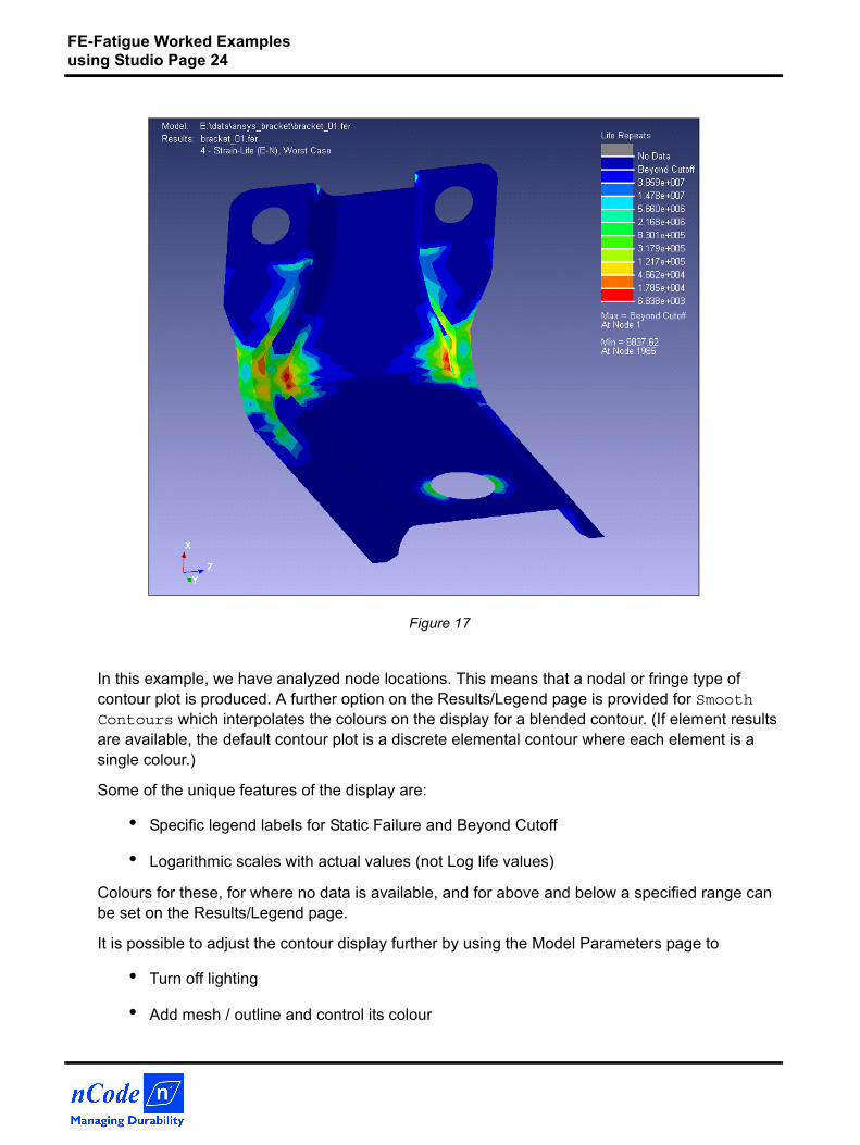
In this example, we have analyzed node locations. This means that a nodal or fringe type of contour plot is produced. A further option on the Results/Legend page is provided for SmoothContours which interpolates the colours on the display for a blended contour. (If element results are available, the default contour plot is a discrete elemental contour where each element is a single colour.)
Some of the unique features of the display are:
• Specific legend labels for Static Failure and Beyond Cutoff
• Logarithmic scales with actual values (not Log life values)
Colours for these, for where no data is available, and for above and below a specified range can be set on the Results/Legend page.
It is possible to adjust the contour display further by using the Model Parameters page to
• Turn off lighting
• Add mesh / outline and control its colour
FE-Fatigue Worked Examples using Studio Page 25
Figure 18
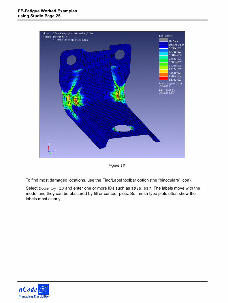
To find most damaged locations, use the Find/Label toolbar option (the “binoculars” icon).
Select Node by ID and enter one or more IDs such as 1985, 617. The labels move with the model and they can be obscured by fill or contour plots. So, mesh type plots often show the labels most clearly.
FE-Fatigue Worked Examples using Studio Page 26
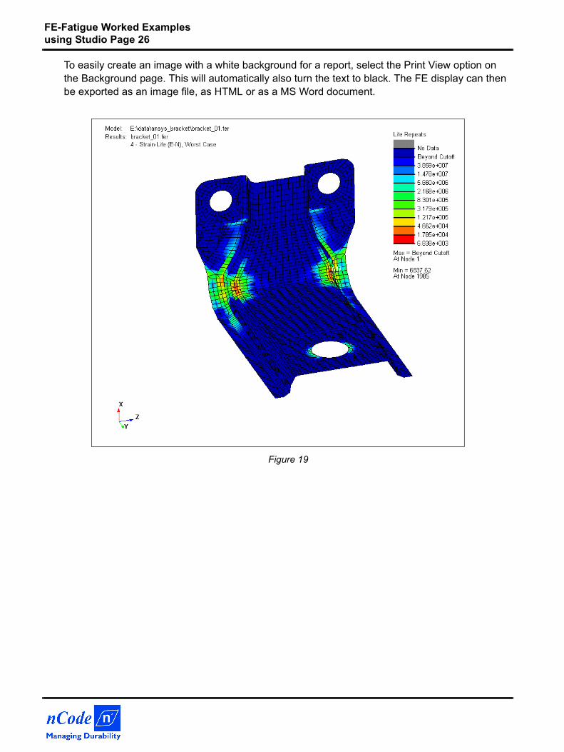
To easily create an image with a white background for a report, select the Print View option on the Background page. This will automatically also turn the text to black. The FE display can then be exported as an image file, as HTML or as a MS Word document.
Figure 19
FE-Fatigue Worked Examples using Studio Page 27
2. Simple S-N Example – Bracket analysisIn this example, you will use the Stress-Life (S-N) approach to calculate the fatigue life for the constant amplitude loading of a bracket. The S-N approach typically relates nominal stresses to total failure and is suited primarily to ‘long-life’ problems where there are a large number of cycles to failure (> 103 or 104 cycles).
This example uses nCode’s Studio FE Display to show the model and results and uses the FE2FES translator to read the stresses from an ANSYS bracket.rst file.
2.1 IntroductionThis example has a bracket bolted to a box section. A vertical load is applied to the end of the bracket. This example will calculate how many times this load can be cycled (+/-) before failure will occur. Exact fatigue material properties of the steel are unknown and will be estimated from known data such as UTS (ultimate tensile strength).
The following file is required for this example:
bracket.rst
It is suggested you copy this files to a new directory before beginning this exercise.
FE-Fatigue Worked Examples using Studio Page 28
2.2 Displaying the model in StudioTo view the model prior to starting the analysis, we will use the nSoft Studio module.
• Start the main nSoft interface, select Display from the nSoft Menu, and select Studio Display/Reporting Tool (studio)
Studio will start and show an empty display area. To insert the model on the display page:
• Select Insert > FE Display
• In the file selection form, select bracket.rst from the working directory and click on Open.
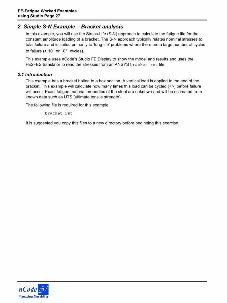
The model is shown on the current Studio page.
Figure 20 ANSYS model displayed using Studio
FE-Fatigue Worked Examples using Studio Page 29
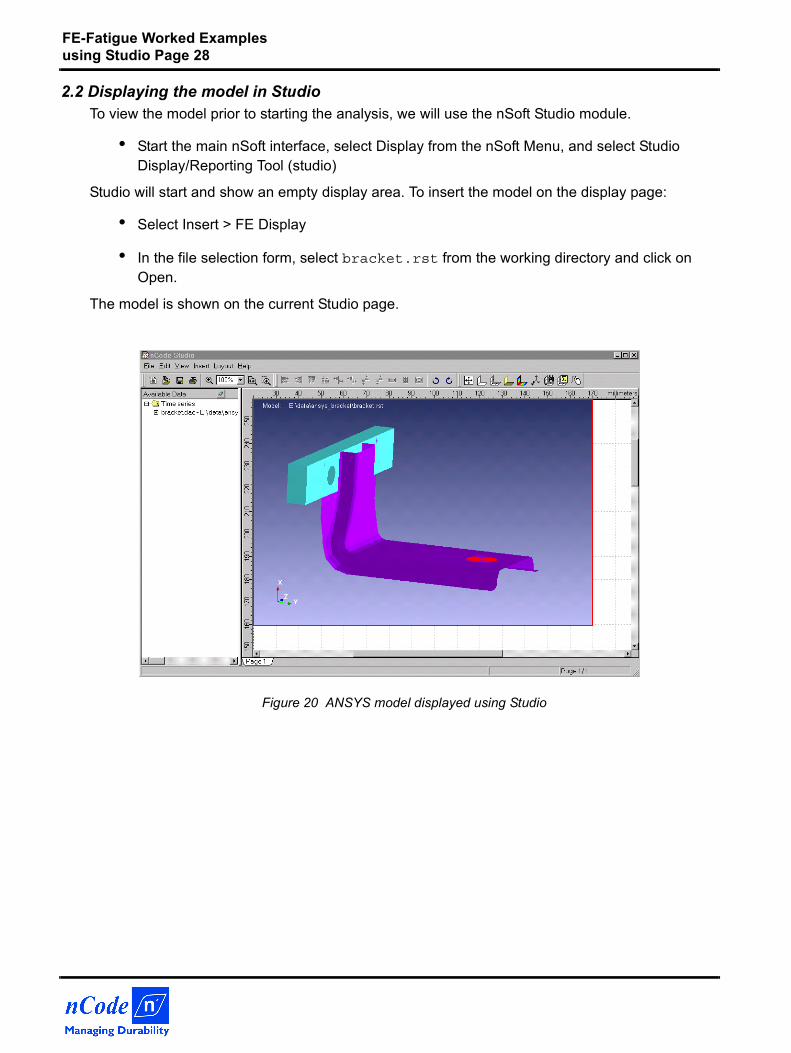
2.3 Translating ANSYS results using FE2ESThe next step is the read the stress data from the ANSYS results .rst file and convert this to a FES file input deck for FE-Fatigue. We will use nCode’s FE translator program, fe2fes.
• Start the main nSoft interface, select FE-Fatigue from the nSoft Menu, and select Generic FE to FES Translator (fe2fes)
fe2fes takes the user through a wizard-style interface to select which entities and which results from an FE Analysis are to be used in a fatigue analysis.
On the first fe2fes form:
• Select Filename: bracket.rst
• Translator: Select translator from file extension (Or ANSYS rst)
Figure 21 FE2FES: File selection
FE-Fatigue Worked Examples using Studio Page 30
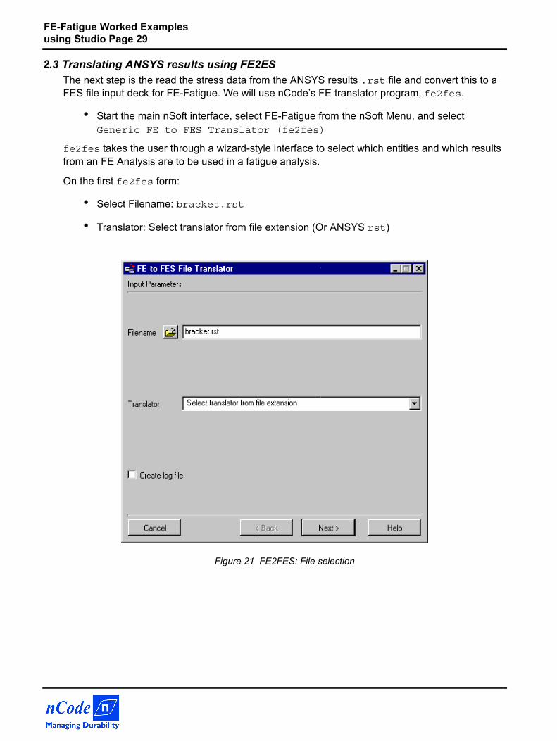
2.4 Group selectionThe first part of the form is the name and type of the FES file to be created.
• Output Filename: bracket_01
• File Type: Binary
This creates a binary FES file, bracket_01.fes.
On the Group Selection form, the part of the model for fatigue analysis is selected by either Property or Material IDs.
The nodal data from shell elements are selected by:
• Solution Location: Element
• Group Type: Material
The Available Groups column lists all the property IDs found in the rst file. Select by clicking on the bracket group:
• 1-MAT_1
and click the -> button to move it to the Selected Groups list.
Figure 22 FE2FES: Group selection
FE-Fatigue Worked Examples using Studio Page 31
The “Combine selected groups into a single group in FES file” option can be checked if you wish to make it easier to use the same fatigue properties across a whole model.
Click the ungreyed Next > button to move on to the next form. (You can also back up at any stage using < Back.)
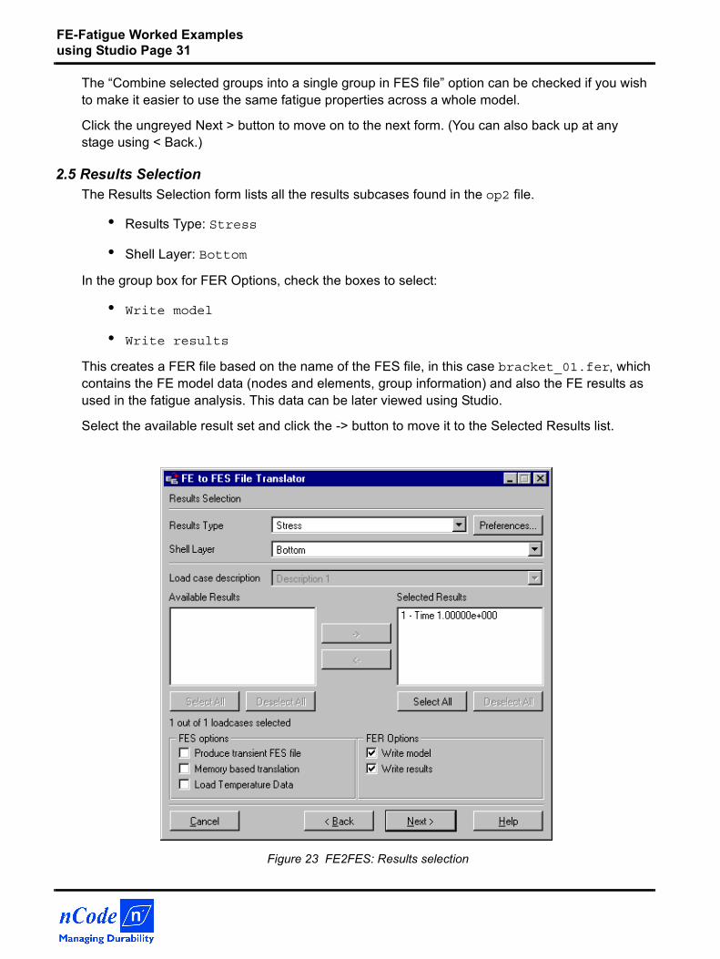
2.5 Results SelectionThe Results Selection form lists all the results subcases found in the op2 file.
• Results Type: Stress
• Shell Layer: Bottom
In the group box for FER Options, check the boxes to select:
• Write model
• Write results
This creates a FER file based on the name of the FES file, in this case bracket_01.fer, which contains the FE model data (nodes and elements, group information) and also the FE results as used in the fatigue analysis. This data can be later viewed using Studio.
Select the available result set and click the -> button to move it to the Selected Results list.
Figure 23 FE2FES: Results selection
FE-Fatigue Worked Examples using Studio Page 32
The final form is a summary of the translation.
Check the “Start FE-Fatigue with FES file” box and click on Finish and the fatfe FE-Fatigue solver program is shown. (Alternatively, you can start fatfe separately and select bracket_01.fes as the Input Fatigue Filename.)
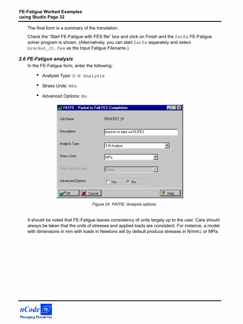
2.6 FE-Fatigue analysisIn the FE-Fatigue form, enter the following:
• Analysis Type: S-N Analysis
• Stress Units: MPa
• Advanced Options: No
Figure 24 FATFE: Analysis options
It should be noted that FE-Fatigue leaves consistency of units largely up to the user. Care should always be taken that the units of stresses and applied loads are consistent. For instance, a model with dimensions in mm with loads in Newtons will by default produce stresses in N/mm2 or MPa.
FE-Fatigue Worked Examples using Studio Page 33
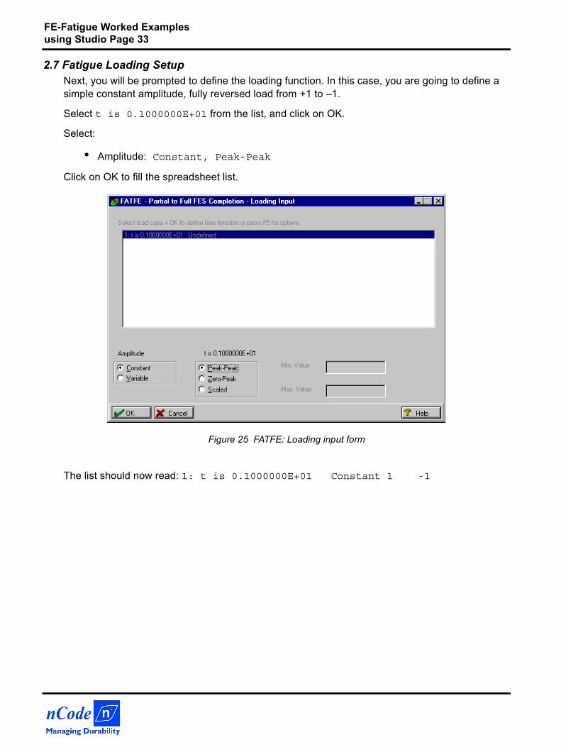
2.7 Fatigue Loading SetupNext, you will be prompted to define the loading function. In this case, you are going to define a simple constant amplitude, fully reversed load from +1 to –1.
Select t is 0.1000000E+01 from the list, and click on OK.
Select:
• Amplitude: Constant, Peak-Peak
Click on OK to fill the spreadsheet list.
Figure 25 FATFE: Loading input form
The list should now read: 1: t is 0.1000000E+01 Constant 1 -1
FE-Fatigue Worked Examples using Studio Page 34
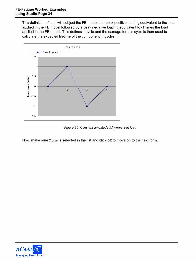
This definition of load will subject the FE model to a peak positive loading equivalent to the load applied in the FE model followed by a peak negative loading equivalent to -1 times the load applied in the FE model. This defines 1 cycle and the damage for this cycle is then used to calculate the expected lifetime of the component in cycles.
Figure 26 Constant amplitude fully-reversed load
Now, make sure Done is selected in the list and click OK to move on to the next form.
Peak to peak
-1.5
-1
-0.5
0
0.5
1
1.5
1 2 3 4
Load
sca
le fa
ctor
Peak to peak
FE-Fatigue Worked Examples using Studio Page 35
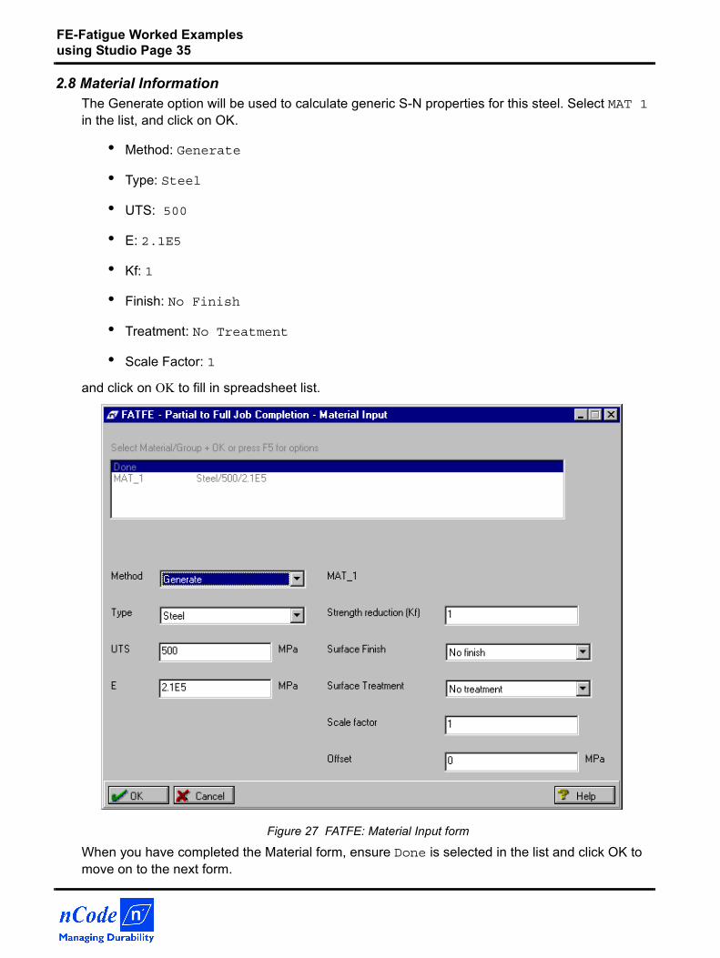
2.8 Material InformationThe Generate option will be used to calculate generic S-N properties for this steel. Select MAT 1 in the list, and click on OK.
• Method: Generate
• Type: Steel
• UTS: 500
• E: 2.1E5
• Kf: 1
• Finish: No Finish
• Treatment: No Treatment
• Scale Factor: 1
and click on OK to fill in spreadsheet list.
Figure 27 FATFE: Material Input form
When you have completed the Material form, ensure Done is selected in the list and click OK to move on to the next form.
FE-Fatigue Worked Examples using Studio Page 36
2.9 Running a Fatigue AnalysisThe next question will ask if you want to go ahead and run the analysis – answer Yes. On the Fatigue Analysis form, accept the defaults:
• Analysis Region: All Data in FES file
• Equivalent Units: 1 Repeats
• Safety Factor Analysis: None
Click on OK. At the “Results Filename Entry” screen select:
• Results Filename: bracket_01
• Output File Format: Default only
• FER File Output: 2- Add to FER file (name as FES)
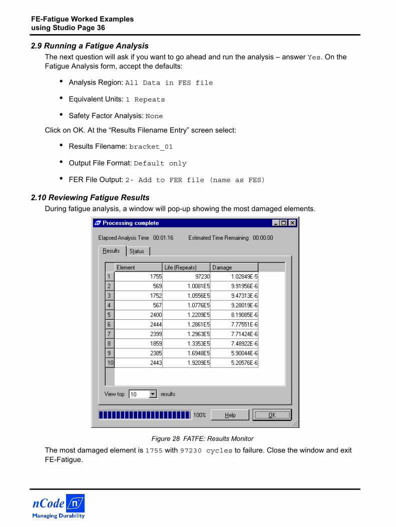
2.10 Reviewing Fatigue ResultsDuring fatigue analysis, a window will pop-up showing the most damaged elements.
Figure 28 FATFE: Results Monitor
The most damaged element is 1755 with 97230 cycles to failure. Close the window and exit FE-Fatigue.
FE-Fatigue Worked Examples using Studio Page 37
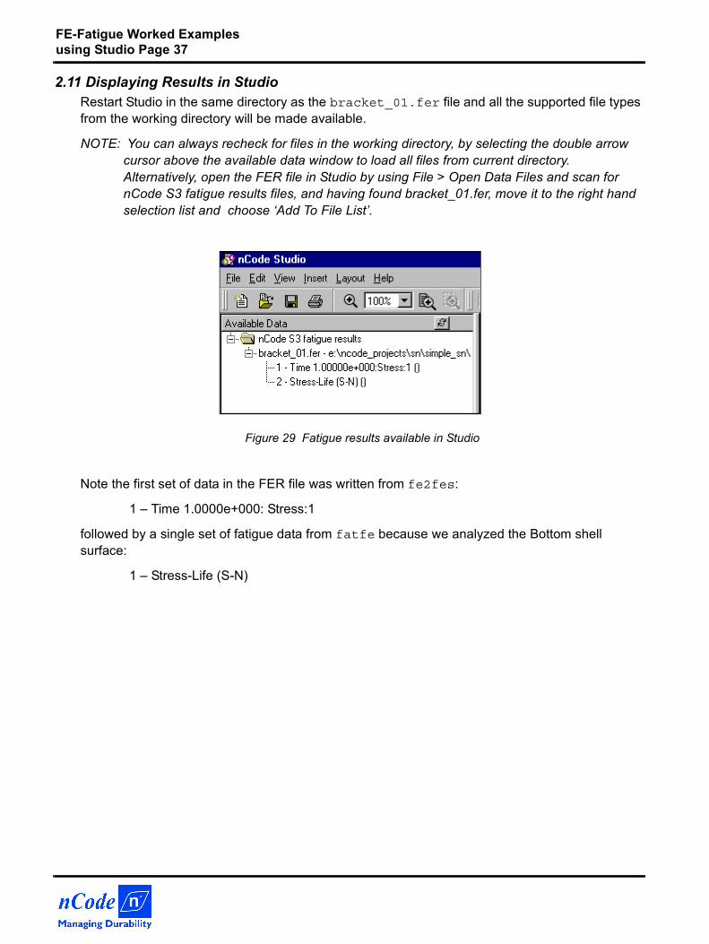
2.11 Displaying Results in StudioRestart Studio in the same directory as the bracket_01.fer file and all the supported file types from the working directory will be made available.
NOTE: You can always recheck for files in the working directory, by selecting the double arrow cursor above the available data window to load all files from current directory. Alternatively, open the FER file in Studio by using File > Open Data Files and scan for nCode S3 fatigue results files, and having found bracket_01.fer, move it to the right hand selection list and choose ‘Add To File List’.
Figure 29 Fatigue results available in Studio
Note the first set of data in the FER file was written from fe2fes:
1 – Time 1.0000e+000: Stress:1
followed by a single set of fatigue data from fatfe because we analyzed the Bottom shell surface:
1 – Stress-Life (S-N)
FE-Fatigue Worked Examples using Studio Page 38
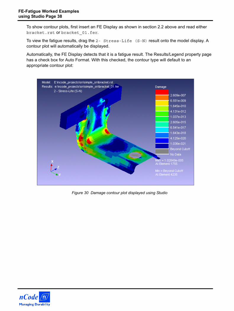
To show contour plots, first insert an FE Display as shown in section 2.2 above and read either bracket.rst or bracket_01.fer.
To view the fatigue results, drag the 2- Stress-Life (S-N) result onto the model display. A contour plot will automatically be displayed.
Automatically, the FE Display detects that it is a fatigue result. The Results/Legend property page has a check box for Auto Format. With this checked, the contour type will default to an appropriate contour plot:
Figure 30 Damage contour plot displayed using Studio
FE-Fatigue Worked Examples using Studio Page 39
3. Multiple Loads ExampleThis example introduces multiple simultaneous loads in a fatigue analysis. The principle of linear superposition is used in the fatigue analysis to combine stresses from finite element analysis with loading time histories. This approach is useful for simulating multiple loads on structures where the dynamic (resonant) effects of the structure can be ignored. This is a widely used method in the automotive industry. This example also includes re-analysis options and methods for speeding up the analysis process.
3.1 IntroductionA front rail and shock tower section of a vehicle structure is subjected to 3 loads (x,y,z) using FE analysis. The FE loads are applied as separate subcases to give the resulting stress due to each load. Measured time history loads (load01.dac, load02.dac, load03.dac) define the loading and a strain-life analysis will be performed for the shock tower using material properties defined by the user.
The following files are required for this example from the demo directory:
shock.datshock.op2load01.dacload02.dacload03.dacshortload.rsp
It is suggested you copy these files to a new directory before beginning this exercise.

FE-Fatigue Worked Examples using Studio Page 40
3.2 Displaying the model in StudioIf you wish to view the model before reading the results, you need to create a new FE display in Studio and then import the NASTRAN bulk data file shock.dat.
• Start the main nSoft interface, select Display from the nSoft Menu, and select Studio Display/Reporting Tool (studio)
Studio will start and show an empty display area. To insert the model on the display page:
• Select Insert > FE Display
• In the file selection form, select shock.dat from the working directory and click on Open.
The model is shown on the current Studio page.
Figure 31 Model displayed in Studio (Fill plot with Mesh)
FE-Fatigue Worked Examples using Studio Page 41
3.3 Translating NASTRAN results using FE2FESThe next step is to read the stress data from the NASTRAN results op2 file and convert this to a FES file input deck for FE-Fatigue. To achieve this, we will use nCode’s FE translator program, fe2fes.
fe2fes takes the user through a wizard-style interface to select which entities and which results from an FE Analysis are to be used in a fatigue analysis. NASTRAN op2 files which have been created on either PC or on a UNIX workstation platform can be read by fe2fes.
Figure 32 FE2FES: Input file selection
On the first fe2fes form, enter the following:
• Filename: shock.op2
• Translator: Select translator from file extension (or NASTRAN op2)
Click Next > to move on to the next form.
FE-Fatigue Worked Examples using Studio Page 42
3.4 Group SelectionThe first part of the form is the name and type of the FES file to be created. In this case:
• Output Filename: shock_01
• File Type: Binary
This creates a binary FES file, shock_01.fes.
On the Group Selection form, the part of the model for fatigue analysis is selected by either Property or Material IDs.
The nodal data from shell elements are selected by:
• Solution Location: Element
• Group Type: Material
The Available Groups column lists all the property IDs found in the op2 file. Select by clicking on the bracket group:
• 1-MAT_1
and click the -> button to move it to the Selected Groups list.
Figure 33 FE2FES: Group selection
FE-Fatigue Worked Examples using Studio Page 43
The “Combine selected groups into a single group in FES file” option can be checked if you wish to make it easier to use the same fatigue properties across a whole model.
Click the ungreyed Next > button to move on to the next form. (You can also back up at any stage using < Back.)
3.5 Results SelectionThe Results Selection form lists all the results subcases found in the op2 file.
• Results Type: Stress
• Shell Layer: Bottom(Z1)
In the group box for FER Options, check the boxes to select:
• Write model
• Write results
This creates a FER file based on the name of the FES file, in this case shock_01.fer, which contains the FE model data (nodes and elements, group information) and also the FE results as used in the fatigue analysis. This data can be later viewed using Studio.
Select the available results set and click the -> button to move them to the Selected Results list.
Figure 34 FE2FES: Results selection
Click Next > to move on to the next form.
FE-Fatigue Worked Examples using Studio Page 44
The final form is a summary of the translation.
Check the “Start FE-Fatigue with FES file” box and click on Finish and the fatfe FE-Fatigue solver program is shown. (Alternatively, you can start fatfe separately and select shock_01.fes as the Input Fatigue Filename.)
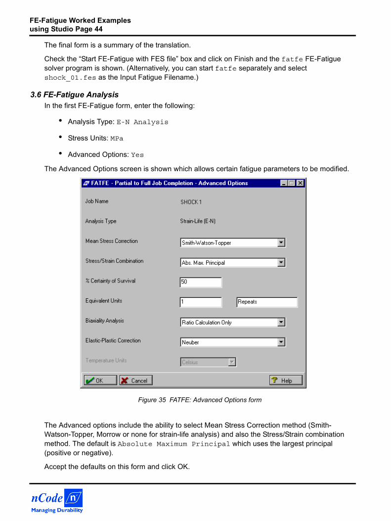
3.6 FE-Fatigue AnalysisIn the first FE-Fatigue form, enter the following:
• Analysis Type: E-N Analysis
• Stress Units: MPa
• Advanced Options: Yes
The Advanced Options screen is shown which allows certain fatigue parameters to be modified.
Figure 35 FATFE: Advanced Options form
The Advanced options include the ability to select Mean Stress Correction method (Smith-Watson-Topper, Morrow or none for strain-life analysis) and also the Stress/Strain combination method. The default is Absolute Maximum Principal which uses the largest principal (positive or negative).
Accept the defaults on this form and click OK.
FE-Fatigue Worked Examples using Studio Page 45
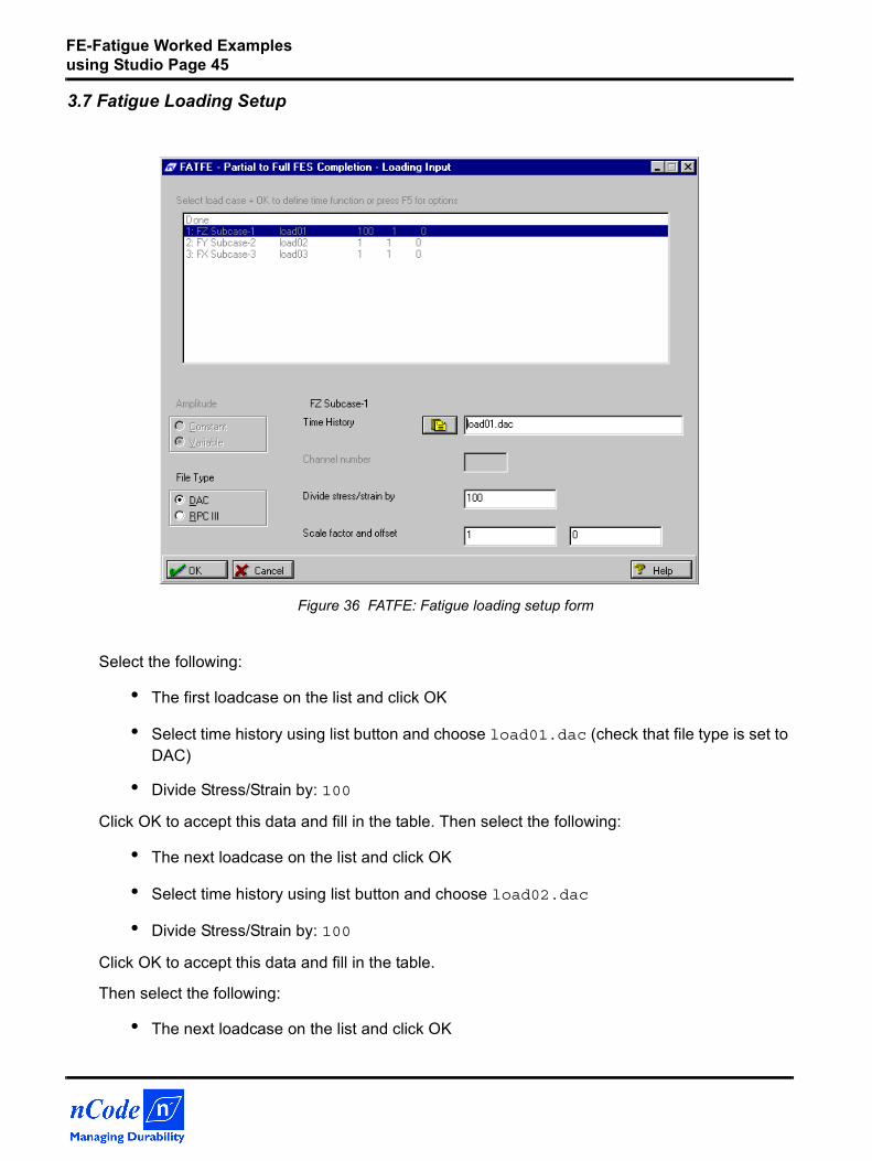
3.7 Fatigue Loading Setup
Figure 36 FATFE: Fatigue loading setup form
Select the following:
• The first loadcase on the list and click OK
• Select time history using list button and choose load01.dac (check that file type is set to DAC)
• Divide Stress/Strain by: 100
Click OK to accept this data and fill in the table. Then select the following:
• The next loadcase on the list and click OK
• Select time history using list button and choose load02.dac
• Divide Stress/Strain by: 100
Click OK to accept this data and fill in the table.
Then select the following:
• The next loadcase on the list and click OK
FE-Fatigue Worked Examples using Studio Page 46
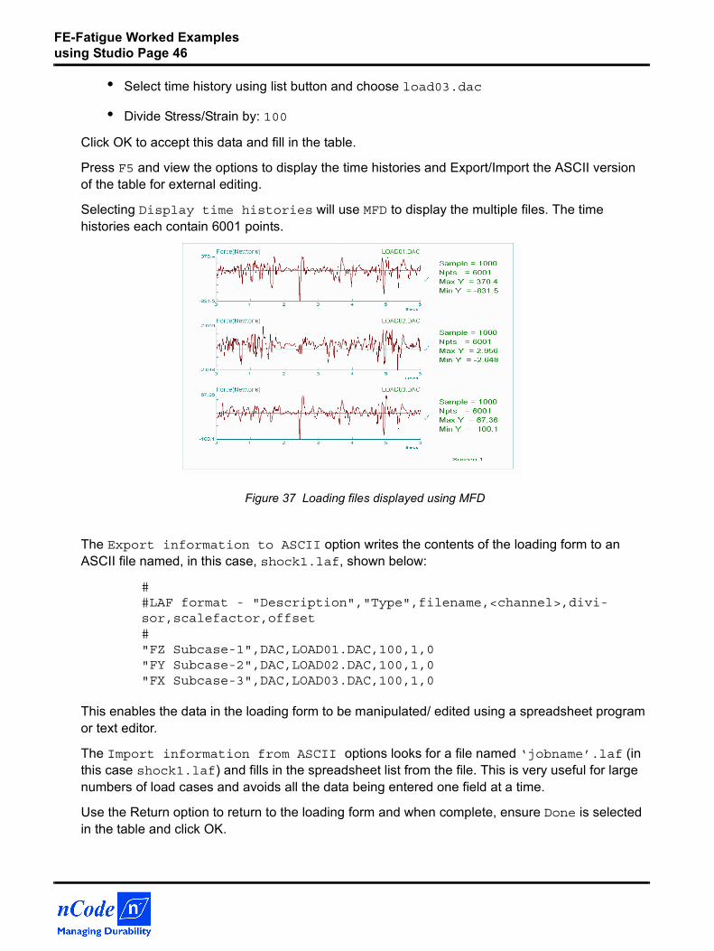
• Select time history using list button and choose load03.dac
• Divide Stress/Strain by: 100
Click OK to accept this data and fill in the table.
Press F5 and view the options to display the time histories and Export/Import the ASCII version of the table for external editing.
Selecting Display time histories will use MFD to display the multiple files. The time histories each contain 6001 points.
Figure 37 Loading files displayed using MFD
The Export information to ASCII option writes the contents of the loading form to an ASCII file named, in this case, shock1.laf, shown below:
##LAF format - "Description","Type",filename,<channel>,divi-sor,scalefactor,offset#"FZ Subcase-1",DAC,LOAD01.DAC,100,1,0"FY Subcase-2",DAC,LOAD02.DAC,100,1,0"FX Subcase-3",DAC,LOAD03.DAC,100,1,0
This enables the data in the loading form to be manipulated/ edited using a spreadsheet program or text editor.
The Import information from ASCII options looks for a file named ‘jobname’.laf (in this case shock1.laf) and fills in the spreadsheet list from the file. This is very useful for large numbers of load cases and avoids all the data being entered one field at a time.
Use the Return option to return to the loading form and when complete, ensure Done is selected in the table and click OK.
FE-Fatigue Worked Examples using Studio Page 47
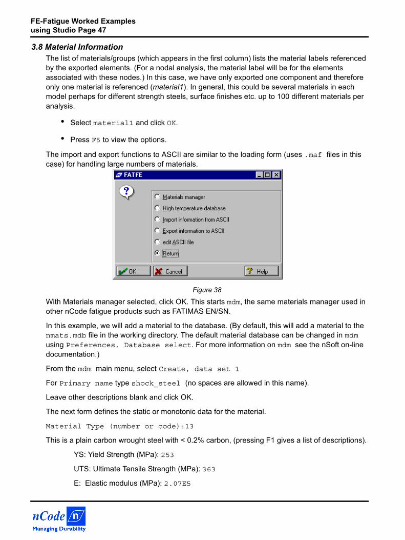
3.8 Material InformationThe list of materials/groups (which appears in the first column) lists the material labels referenced by the exported elements. (For a nodal analysis, the material label will be for the elements associated with these nodes.) In this case, we have only exported one component and therefore only one material is referenced (material1). In general, this could be several materials in each model perhaps for different strength steels, surface finishes etc. up to 100 different materials per analysis.
• Select material1 and click OK.
• Press F5 to view the options.
The import and export functions to ASCII are similar to the loading form (uses .maf files in this case) for handling large numbers of materials.
Figure 38
With Materials manager selected, click OK. This starts mdm, the same materials manager used in other nCode fatigue products such as FATIMAS EN/SN.
In this example, we will add a material to the database. (By default, this will add a material to the nmats.mdb file in the working directory. The default material database can be changed in mdm using Preferences, Database select. For more information on mdm see the nSoft on-line documentation.)
From the mdm main menu, select Create, data set 1
For Primary name type shock_steel (no spaces are allowed in this name).
Leave other descriptions blank and click OK.
The next form defines the static or monotonic data for the material.
Material Type (number or code):13
This is a plain carbon wrought steel with < 0.2% carbon, (pressing F1 gives a list of descriptions).
YS: Yield Strength (MPa): 253
UTS: Ultimate Tensile Strength (MPa): 363
E: Elastic modulus (MPa): 2.07E5
FE-Fatigue Worked Examples using Studio Page 48
Leave the rest blank and click OK.
The next form is for the strain-life (E-N) fatigue data. Enter the following data:
Sf': Fatigue strength coefficient (MPa) 1297
b: Fatigue strength exponent -0.18
c: Fatigue ductility exponent -0.59
Ef': Fatigue ductility coefficient 0.93
n': Cyclic strain-hardening exponent 0.35
K': Cyclic strength coefficient (MPa) 1953
Nc: Cut-off (reversals) 2E8
SEe: Standard Error of Log(e) (Elastic) 0
SEp: Standard Error of Log(e) (Plastic) 0
SEc: Standard Error of Log(e) (Cyclic) 0
Click OK to accept this form; OK all subsequent forms to enter the material into the database.
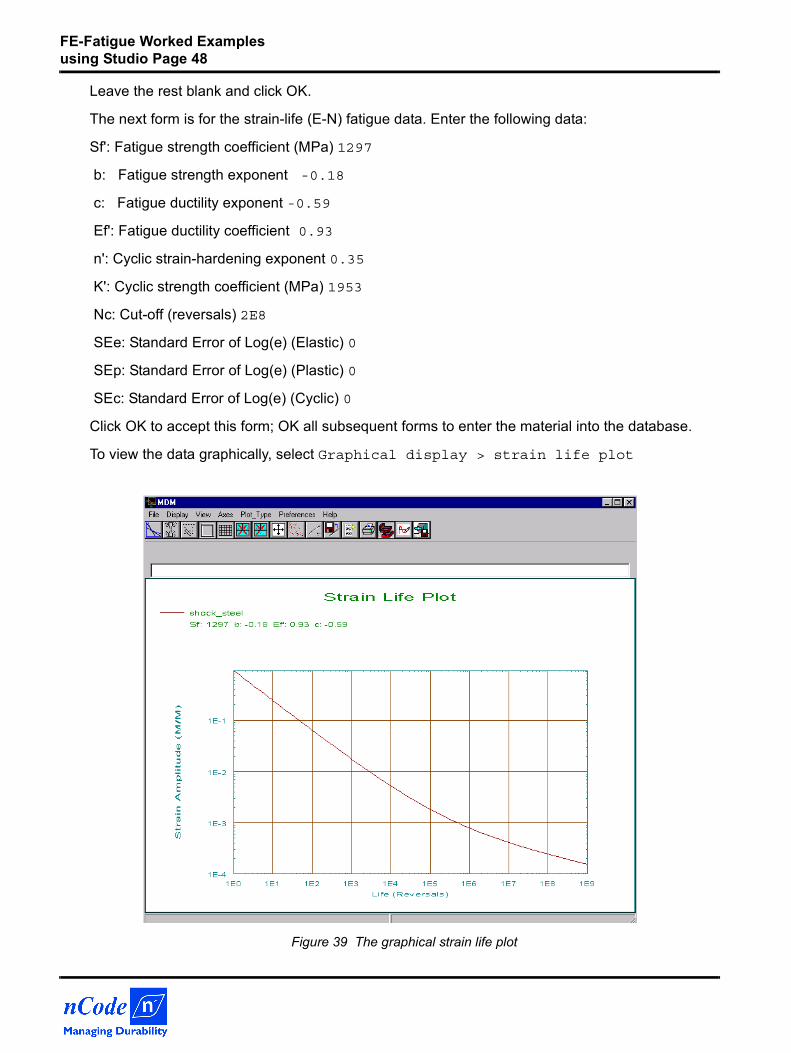
To view the data graphically, select Graphical display > strain life plot
Figure 39 The graphical strain life plot
FE-Fatigue Worked Examples using Studio Page 49
When complete, exit from the mdm main menu and you will return to the material input form.
With material1 selected, and method set to select, view the list of materials in the database; shock_steel should be now on the list. Select shock_steel and accept the other defaults. Click OK to accept this data and fill in the table.
When all of the above stages are complete, select Done in the list and click OK.
3.9 Running a Fatigue AnalysisEnter the following details:
• Analysis Region: All data in FES file
• Equivalent Units: 1 Repeats
• Safety Factor Analysis: None
Click on OK.
In the Results Filename screen select:
• Results Filename: shock_01
• Shell calculation: Worst
• Output File Format: Default only
• FER File Output: 2- Add to FER file (name as FES)
The analysis takes a few minutes and on completion the summary of results should show the most damaged element to be 26283, with 1164 repeats.
FE-Fatigue Worked Examples using Studio Page 50
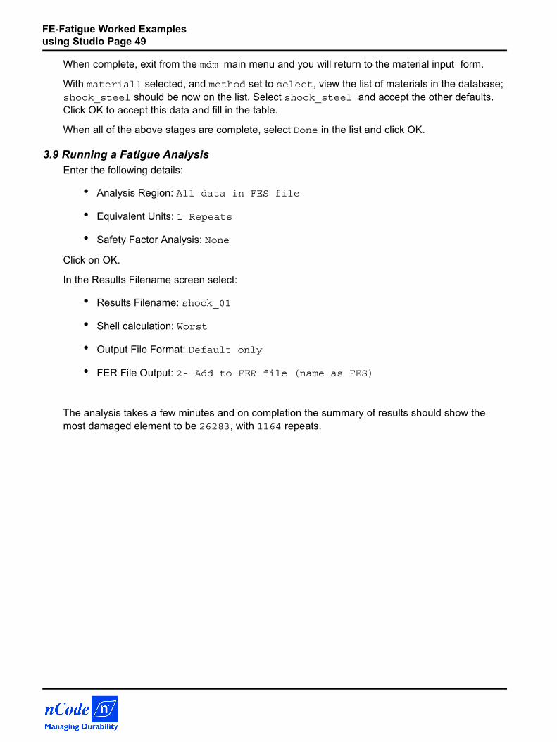
3.10 Displaying Results in StudioRestart Studio in the same directory as the shock_01.fer file and all the supported file types from the working directory will be made available.
NOTE: You can always recheck for files in the working directory, by selecting the double arrow cursor above the available data window to load all files from current directory. Alternatively, open the FER file in Studio by using File > Open Data Files and scan for nCode S3 fatigue results files, and having found shock_01.fer, move it to the right hand selection list and choose ‘Add To File List’.
Figure 40 Fatigue results files available in Studio
Note that three sets of data in the FER file were written from fe2fes, corresponding to the three load cases:
1 – FZ=1000 N: Stress:1
2 – FZ=1000 N: Stress:2
3 – FZ=1000 N: Stress:3
followed by a single set of fatigue data from fatfe because we analyzed the Bottom shell surface:
4 – Strain-Life (S-N)
FE-Fatigue Worked Examples using Studio Page 51
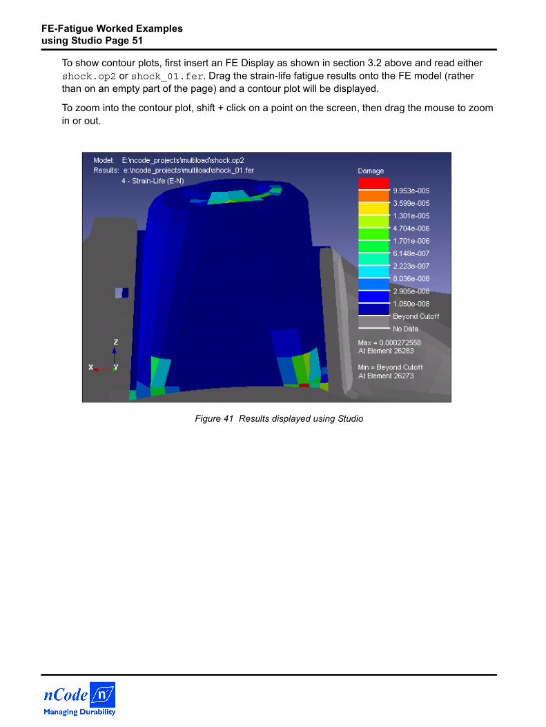
To show contour plots, first insert an FE Display as shown in section 3.2 above and read either shock.op2 or shock_01.fer. Drag the strain-life fatigue results onto the FE model (rather than on an empty part of the page) and a contour plot will be displayed.
To zoom into the contour plot, shift + click on a point on the screen, then drag the mouse to zoom in or out.
Figure 41 Results displayed using Studio
FE-Fatigue Worked Examples using Studio Page 52
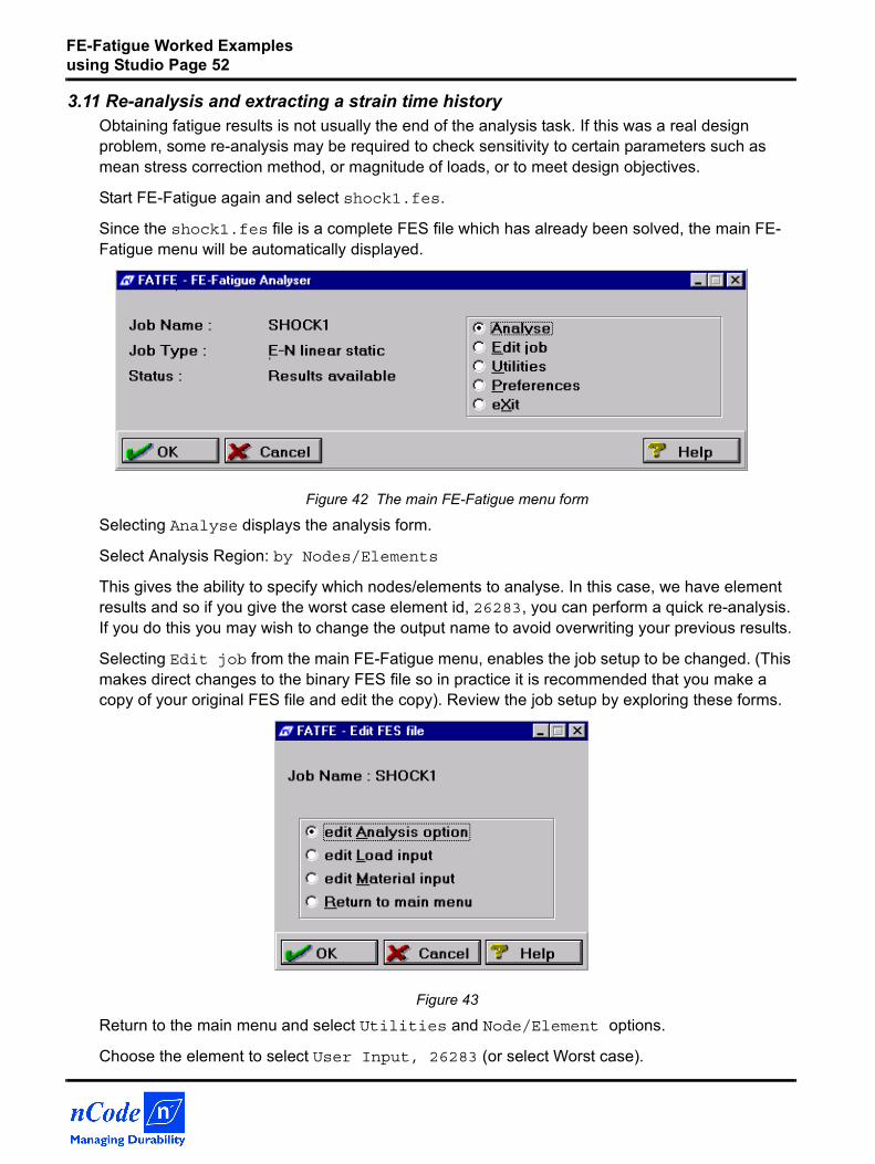
3.11 Re-analysis and extracting a strain time history Obtaining fatigue results is not usually the end of the analysis task. If this was a real design problem, some re-analysis may be required to check sensitivity to certain parameters such as mean stress correction method, or magnitude of loads, or to meet design objectives.
Start FE-Fatigue again and select shock1.fes.
Since the shock1.fes file is a complete FES file which has already been solved, the main FE-Fatigue menu will be automatically displayed.
Figure 42 The main FE-Fatigue menu form
Selecting Analyse displays the analysis form.
Select Analysis Region: by Nodes/Elements
This gives the ability to specify which nodes/elements to analyse. In this case, we have element results and so if you give the worst case element id, 26283, you can perform a quick re-analysis. If you do this you may wish to change the output name to avoid overwriting your previous results.
Selecting Edit job from the main FE-Fatigue menu, enables the job setup to be changed. (This makes direct changes to the binary FES file so in practice it is recommended that you make a copy of your original FES file and edit the copy). Review the job setup by exploring these forms.
Figure 43
Return to the main menu and select Utilities and Node/Element options.
Choose the element to select User Input, 26283 (or select Worst case).
FE-Fatigue Worked Examples using Studio Page 53
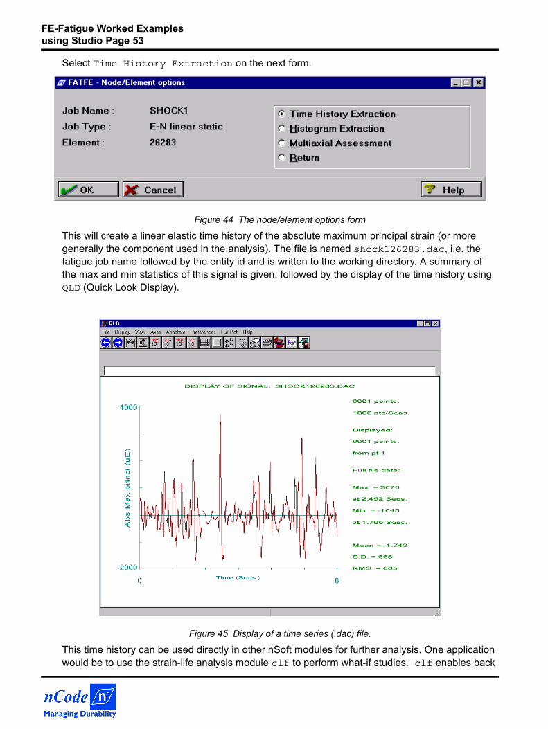
Select Time History Extraction on the next form.
Figure 44 The node/element options form
This will create a linear elastic time history of the absolute maximum principal strain (or more generally the component used in the analysis). The file is named shock126283.dac, i.e. the fatigue job name followed by the entity id and is written to the working directory. A summary of the max and min statistics of this signal is given, followed by the display of the time history using QLD (Quick Look Display).
Figure 45 Display of a time series (.dac) file.
This time history can be used directly in other nSoft modules for further analysis. One application would be to use the strain-life analysis module clf to perform what-if studies. clf enables back
FE-Fatigue Worked Examples using Studio Page 54
calculations to be performed to find out which parameters would achieve a certain life. It also creates damage matrices to identify how much damage is attributable to which size of cycles in the time history.
Currently, care must be taken to redefine the fatigue parameters in clf to be the same as in FE-Fatigue, and since FE-Fatigue calculates lives from a rainflow matrix rather than a time history, the resulting lives can be slightly different. Results should however agree if a rainflow matrix is exported from FE-Fatigue and used in clf.
3.12 Accelerating the ProcessThe two main contributors to fatigue analysis run-time are:
• Number of Nodes/Elements to analyse
• Number of points in the loading time histories (time steps)
In this shock tower example, the FE mesh is probably too coarse to achieve good stress results and as meshes become finer so run times increase. Also time histories can be much longer than the 6 seconds used in this case.
To shorten the time histories module pvxmul is provided. This performs peak valley slicing on multiple time histories. It relies on the principle that fatigue is only dependant on cycles and reduces each loading time history (channel) to a peak-valley sequence. The phase relationship is maintained by retaining points in all the channels if a turning point (maxima or minima) occurs in any of the channels.
Since this approach removes the time content (and hence frequency content) this is only valid for quasi-static type analysis where there are no resonance effects.
To run pvxmul, load nSoft by typing nsoft5 at the unix prompt, or from the NT Start menu.
Within nSoft5 select Peak Valley Slicing (pvxmul) from the FE-Fatigue menu or type pvxmul at the prompt.
• Input File Type: DAC
• Generic Input Filename: load (and press OK)
• Channels: ALL
• Output Filename: load
• Write time file: No
NOTE: The loading time histories need to use this naming convention of a filename stem (in this case load) followed by a channel number (01,02,03 etc.).
Click OKand on the next form select:
• Gate Method: Cycles
Clicking OK will start a spreadsheet to input a gate threshold. This is most easily defined as a percentage of the largest cycle in each channel.
FE-Fatigue Worked Examples using Studio Page 55
• For Channel 1, select the cell in column G (% Gate) and enter 5.
• Repeat this action for other channels, or to speed things up press copy to fill down.
• Select File, OK to begin the peak valley slicing.
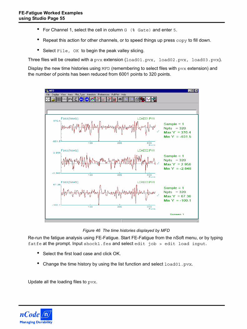
Three files will be created with a pvx extension (load01.pvx, load02.pvx, load03.pvx).
Display the new time histories using MFD (remembering to select files with pvx extension) and the number of points has been reduced from 6001 points to 320 points.
Figure 46 The time histories displayed by MFD
Re-run the fatigue analysis using FE-Fatigue. Start FE-Fatigue from the nSoft menu, or by typing fatfe at the prompt. Input shock1.fes and select edit job > edit load input.
• Select the first load case and click OK.
• Change the time history by using the list function and select load01.pvx.
Update all the loading files to pvx.
FE-Fatigue Worked Examples using Studio Page 56
Alternatively a quicker way could be to edit the shock1.laf file created earlier; text edit shock1.laf and replace all dac by pvx. Use F5 on the loading form to import this ASCII file to update the list.
Click OK to process the loading form to save the changes, and return to the main menu. Select analyse and analyse all data in FES file. Change the results file name to shock1_pvx and run the job. The job should run much quicker than before giving the most damaged element as 26283 with 1165 repeats.
The other main influence on the length of the run time is the number of nodes or elements. FE-Fatigue includes an auto-elimination option to pre-select nodes or elements on which to focus the analysis.
This method exploits the fact that for most structures the high stresses are concentrated in local areas and large proportions of the model experience little or no stress. Auto-elimination uses the magnitude of the stress due to each loadcase and the magnitude of the load to calculate an approximate worst case stress for each node or element. This value of stress is then used to filter out the lower stressed nodes/elements.
From main menu of FE-Fatigue, select Analyse.
• Analysis Region: auto elimination (% model to retain)
• Auto Elimination Retention Factor: 25
• Auto Elimination Stress Threshold: 0 MPa
This will retain 25% of the shock cap for analysis with highest 'total' stresses. This should speed up the analysis by almost 4 times.
Accept other defaults and click OK.
Change the results file name to shock1_auto and run the job. Note that although the analysis is much quicker, the results file and contour plots only contain results for this subset of the model. Results will be identical to the shock1_pvx results since the loading functions used are the same. Use the results listing module fatres (from the FE-Fatigue menu or Utilities >Results listing) to compare shock1_auto.fef and shock1_pvx.fef. These are the ASCII files of the results of each analysis in PATRAN format.
Additionally, a stress threshold can be set which can be used to remove further nodes or elements from the analysis set. This allows an absolute 'fatigue limit', e.g 50 MPa, to be set such that if the estimated worst case stress for a location is below this limit, then that location will not be analysed.
This auto-elimination method is very useful but should be used with caution, especially where a large proportion of the model is being discarded, and where other factors such as mean stresses may increase damage.
FE-Fatigue Worked Examples using Studio Page 57
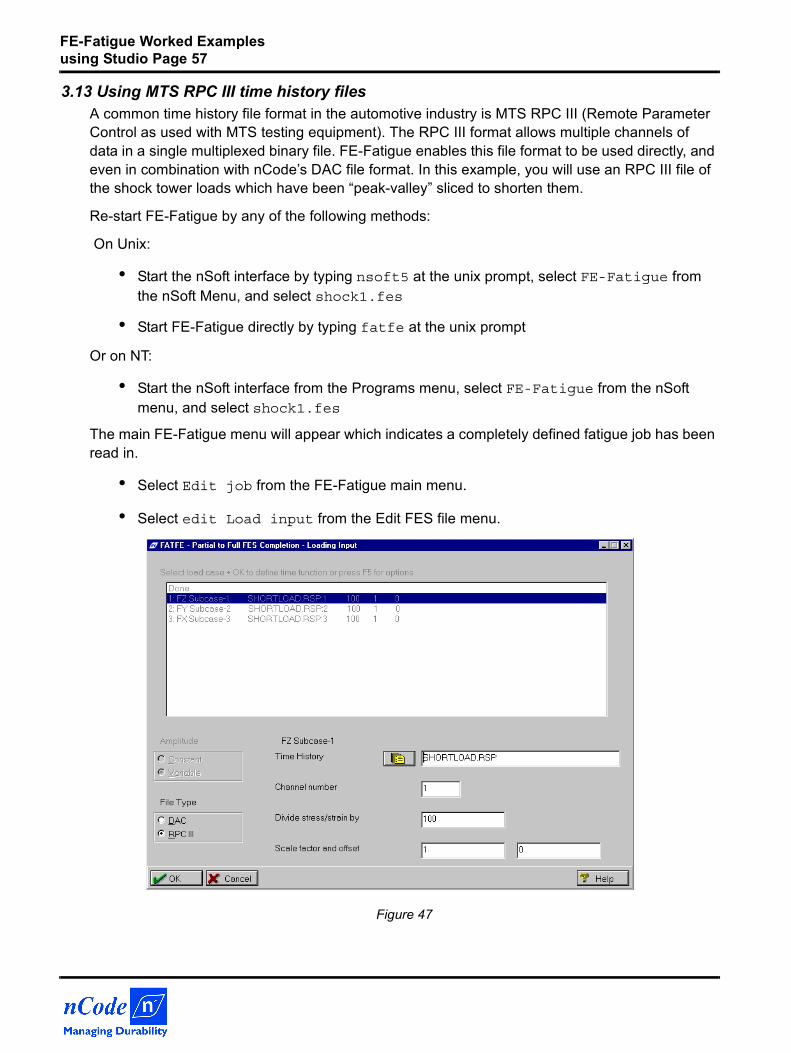
3.13 Using MTS RPC III time history filesA common time history file format in the automotive industry is MTS RPC III (Remote Parameter Control as used with MTS testing equipment). The RPC III format allows multiple channels of data in a single multiplexed binary file. FE-Fatigue enables this file format to be used directly, and even in combination with nCode’s DAC file format. In this example, you will use an RPC III file of the shock tower loads which have been “peak-valley” sliced to shorten them.
Re-start FE-Fatigue by any of the following methods:
On Unix:
• Start the nSoft interface by typing nsoft5 at the unix prompt, select FE-Fatigue from the nSoft Menu, and select shock1.fes
• Start FE-Fatigue directly by typing fatfe at the unix prompt
Or on NT:
• Start the nSoft interface from the Programs menu, select FE-Fatigue from the nSoft menu, and select shock1.fes
The main FE-Fatigue menu will appear which indicates a completely defined fatigue job has been read in.
• Select Edit job from the FE-Fatigue main menu.
• Select edit Load input from the Edit FES file menu.
Figure 47
FE-Fatigue Worked Examples using Studio Page 58
Select:
• The first loadcase on the list and click OK
• File Type: RPC III
• Select time history using the list button and choose shortload.rsp
• Channel number: 1
• Divide stress/strain by: 100
Click OK to accept this data and fill in the table.
Select:
• The next loadcase and click OK
• File Type: RPC III
• Select time history using the list button and choose shortload.rsp
• Channel number: 2
• Divide stress/strain by: 100
Click OK to accept this data and fill in the table.
Select:
• The next loadcase and click OK
• File Type: RPC III
• Select time history using the list button and choose shortload.rsp
• Channel number: 3
• Divide stress/strain by: 100
Click OK to accept this data and fill in the table.
If you are licensed for nCode’s VALIDATA or RIGLINK products, you can directly view/edit RPC III files using the muledt display module. Pressing F5 on the FE-Fatigue loading form will give the option to view time histories. The ASCII export/ import options also directly support RPC files and channel numbers.
If you do not have access to these programs, the nCode STUDIO program can be used to view RPC files.
When completed, ensure Done is selected in the table and click OK.
To submit the fatigue analysis job, select Analyse from the FE-Fatigue main menu.
FE-Fatigue Worked Examples using Studio Page 59
Select / enter the following parameters:
• Analysis region: All data in FES file
• Equivalent units: 1 Repeats
• Safety Factor Analysis : None
And click on OK.
Change the results name from shock1 to shockrpc and click on OK.
The analysis should be relatively quick since the time histories have been edited but should be equivalent to results from the previous exercises.
3.14 Further Comments on Using RPC III FilesIn nSoft V5.3 and FE-Fatigue Release 4 or later versions, support for RPC files by default assumes the standard MTS format. This means that on all platforms, nSoft is able to use RPC files from MTS software without any further translation. In previous versions, RPC files needed to be translated (using CONFIL) from VMS format to the local operating system format.
If users have existing RPC files in local operating system format, it will be necessary to convert these RPC files to MTS format (VMS) using CONFIL. Alternatively, FE-Fatigue can use these local format files if a home environment keyword is set (run the ENM module setting keyword: $RPCOPSY, value: LOCAL). To use MTS format files either remove this keyword or set value to VMS.
There is also the option on the FE-Fatigue Preferences form, to set RPC III as the default time history type rather than DAC; the loading form will then default to RPC III as the loading type.
FE-Fatigue Worked Examples using Studio Page 60
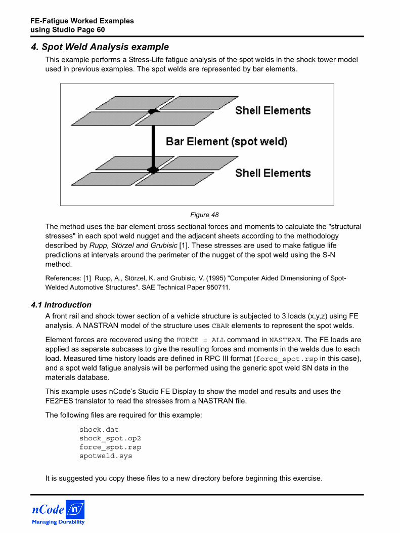
4. Spot Weld Analysis exampleThis example performs a Stress-Life fatigue analysis of the spot welds in the shock tower model used in previous examples. The spot welds are represented by bar elements.
Figure 48
The method uses the bar element cross sectional forces and moments to calculate the "structural stresses" in each spot weld nugget and the adjacent sheets according to the methodology described by Rupp, Störzel and Grubisic [1]. These stresses are used to make fatigue life predictions at intervals around the perimeter of the nugget of the spot weld using the S-N method.
References: [1] Rupp, A., Störzel, K. and Grubisic, V. (1995) "Computer Aided Dimensioning of Spot-Welded Automotive Structures". SAE Technical Paper 950711.
4.1 IntroductionA front rail and shock tower section of a vehicle structure is subjected to 3 loads (x,y,z) using FE analysis. A NASTRAN model of the structure uses CBAR elements to represent the spot welds.
Element forces are recovered using the FORCE = ALL command in NASTRAN. The FE loads are applied as separate subcases to give the resulting forces and moments in the welds due to each load. Measured time history loads are defined in RPC III format (force_spot.rsp in this case), and a spot weld fatigue analysis will be performed using the generic spot weld SN data in the materials database.
This example uses nCode’s Studio FE Display to show the model and results and uses the FE2FES translator to read the stresses from a NASTRAN file.
The following files are required for this example:
shock.datshock_spot.op2force_spot.rspspotweld.sys
It is suggested you copy these files to a new directory before beginning this exercise.
FE-Fatigue Worked Examples using Studio Page 61
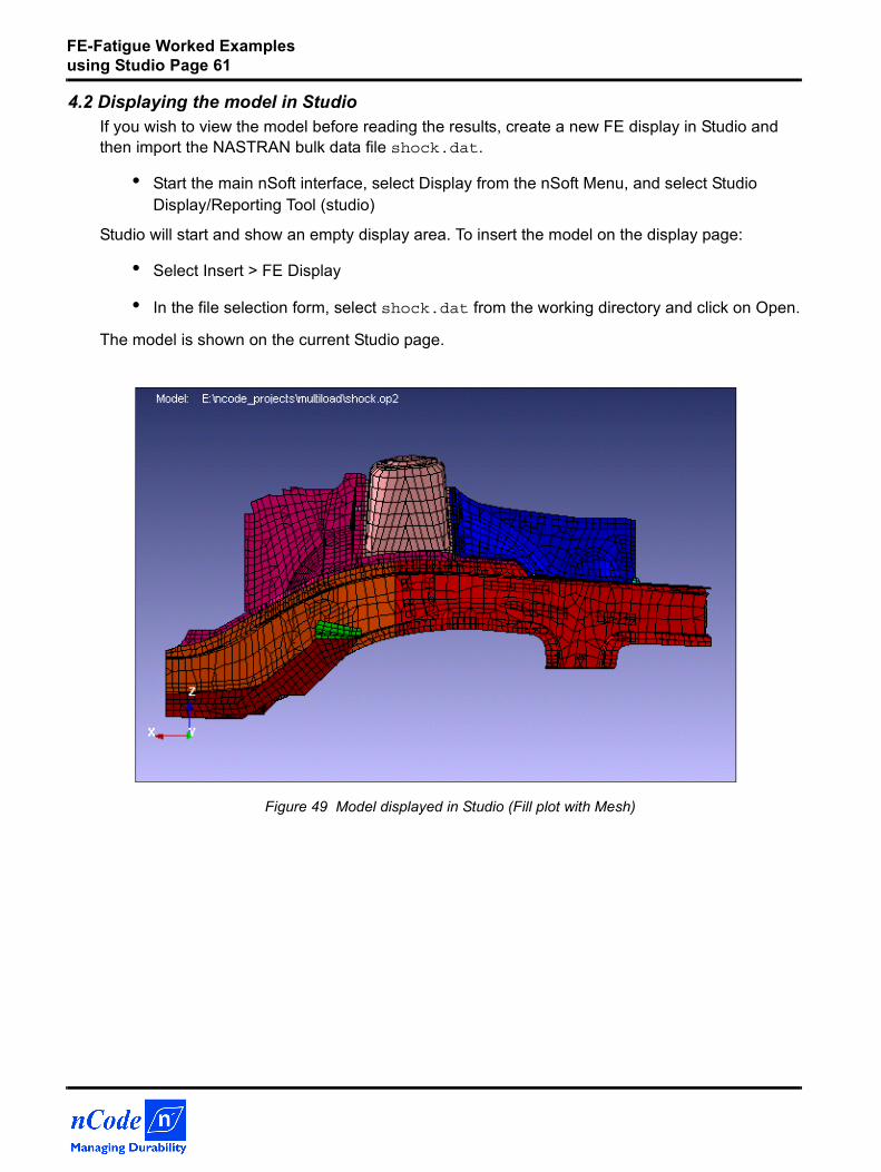
4.2 Displaying the model in StudioIf you wish to view the model before reading the results, create a new FE display in Studio and then import the NASTRAN bulk data file shock.dat.
• Start the main nSoft interface, select Display from the nSoft Menu, and select Studio Display/Reporting Tool (studio)
Studio will start and show an empty display area. To insert the model on the display page:
• Select Insert > FE Display
• In the file selection form, select shock.dat from the working directory and click on Open.
The model is shown on the current Studio page.
Figure 49 Model displayed in Studio (Fill plot with Mesh)
FE-Fatigue Worked Examples using Studio Page 62
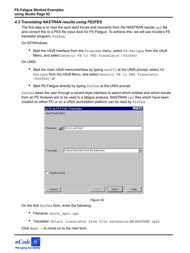
4.3 Translating NASTRAN results using FE2FESThe first step is to read the spot weld forces and moments from the NASTRAN results op2 file and convert this to a FES file input deck for FE-Fatigue. To achieve this, we will use nCode’s FE translator program, fe2fes.
On NT/Windows:
• Start the nSoft interface from the Programs menu, select FE-Fatigue from the nSoft Menu, and select Generic FE to FES Translator (fe2fes)
On UNIX:
• Start the main nSoft menu/interface by typing nsoft5 at the UNIX prompt, select FE-Fatigue from the nSoft Menu, and select Generic FE to FES Translator (fe2fes); or
• Start FE-Fatigue directly by typing fe2fes at the UNIX prompt
fe2fes takes the user through a wizard-style interface to select which entities and which results from an FE Analysis are to be used in a fatigue analysis. NASTRAN op2 files which have been created on either PC or on a UNIX workstation platform can be read by fe2fes.
Figure 50
On the first fe2fes form, enter the following:
• Filename: shock_spot.op2
• Translator: Select translator from file extension (or NASTRAN op2)
Click Next > to move on to the next form.
FE-Fatigue Worked Examples using Studio Page 63
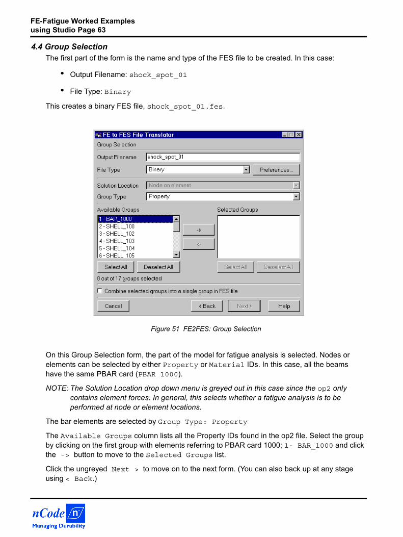
4.4 Group SelectionThe first part of the form is the name and type of the FES file to be created. In this case:
• Output Filename: shock_spot_01
• File Type: Binary
This creates a binary FES file, shock_spot_01.fes.
Figure 51 FE2FES: Group Selection
On this Group Selection form, the part of the model for fatigue analysis is selected. Nodes or elements can be selected by either Property or Material IDs. In this case, all the beams have the same PBAR card (PBAR 1000).
NOTE: The Solution Location drop down menu is greyed out in this case since the op2 only contains element forces. In general, this selects whether a fatigue analysis is to be performed at node or element locations.
The bar elements are selected by Group Type: Property
The Available Groups column lists all the Property IDs found in the op2 file. Select the group by clicking on the first group with elements referring to PBAR card 1000; 1- BAR_1000 and click the -> button to move to the Selected Groups list.
Click the ungreyed Next > to move on to the next form. (You can also back up at any stage using < Back.)
FE-Fatigue Worked Examples using Studio Page 64
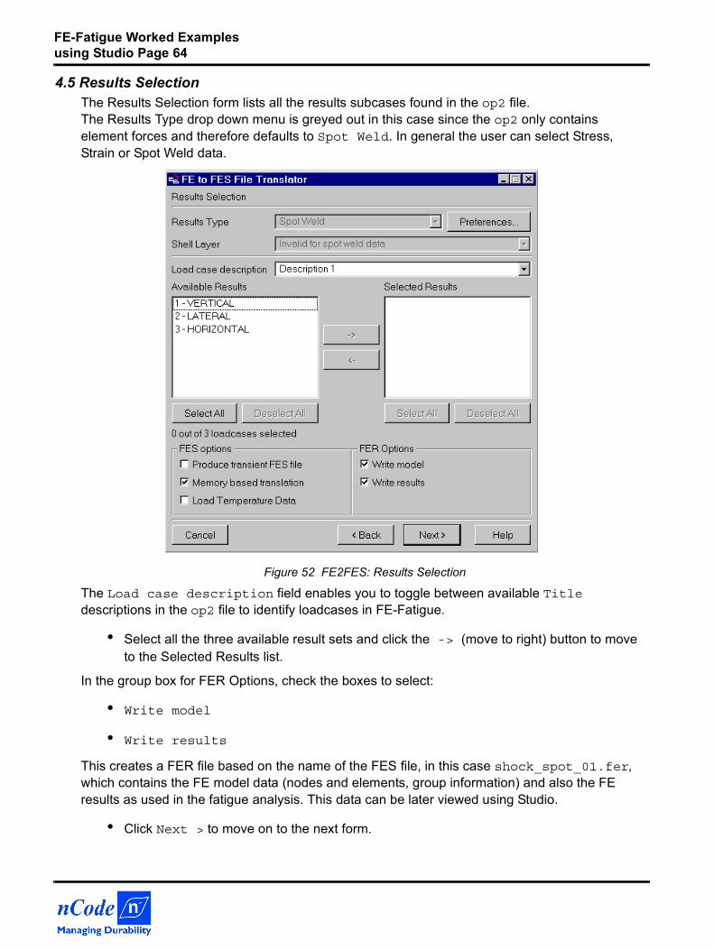
4.5 Results SelectionThe Results Selection form lists all the results subcases found in the op2 file.The Results Type drop down menu is greyed out in this case since the op2 only contains element forces and therefore defaults to Spot Weld. In general the user can select Stress, Strain or Spot Weld data.
Figure 52 FE2FES: Results Selection
The Load case description field enables you to toggle between available Title descriptions in the op2 file to identify loadcases in FE-Fatigue.
• Select all the three available result sets and click the -> (move to right) button to move to the Selected Results list.
In the group box for FER Options, check the boxes to select:
• Write model
• Write results
This creates a FER file based on the name of the FES file, in this case shock_spot_01.fer, which contains the FE model data (nodes and elements, group information) and also the FE results as used in the fatigue analysis. This data can be later viewed using Studio.
• Click Next > to move on to the next form.
FE-Fatigue Worked Examples using Studio Page 65
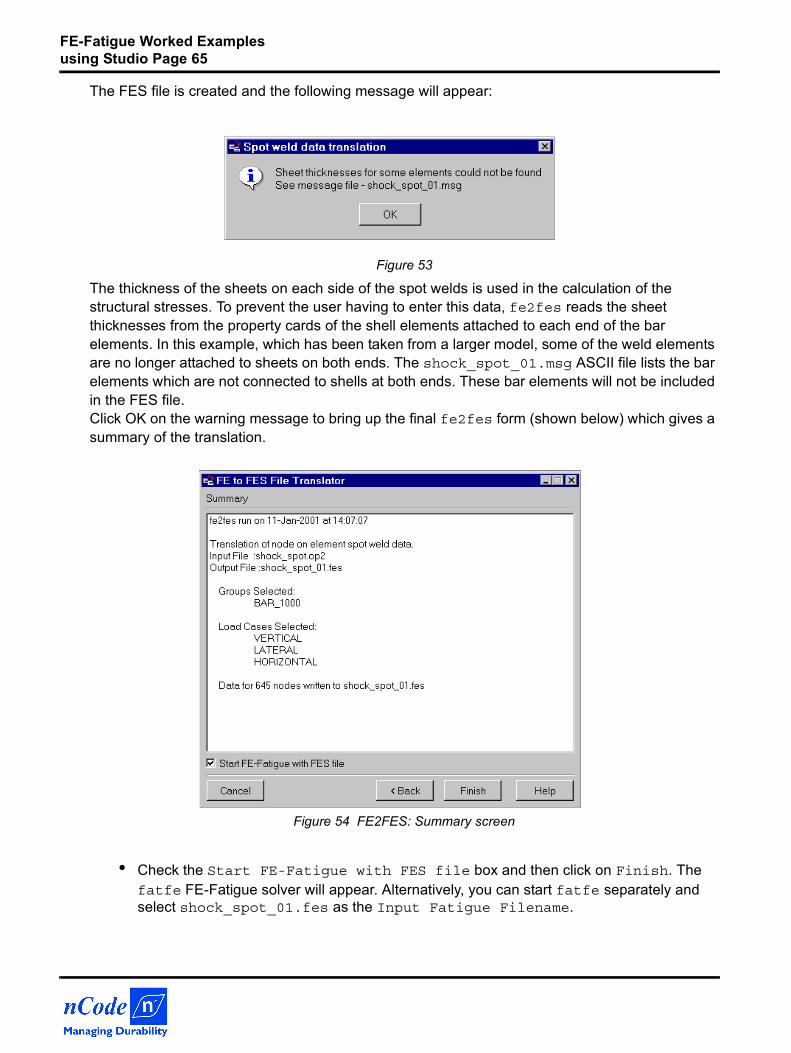
The FES file is created and the following message will appear:
Figure 53
The thickness of the sheets on each side of the spot welds is used in the calculation of the structural stresses. To prevent the user having to enter this data, fe2fes reads the sheet thicknesses from the property cards of the shell elements attached to each end of the bar elements. In this example, which has been taken from a larger model, some of the weld elements are no longer attached to sheets on both ends. The shock_spot_01.msg ASCII file lists the bar elements which are not connected to shells at both ends. These bar elements will not be included in the FES file.Click OK on the warning message to bring up the final fe2fes form (shown below) which gives a summary of the translation.
Figure 54 FE2FES: Summary screen
• Check the Start FE-Fatigue with FES file box and then click on Finish. The fatfe FE-Fatigue solver will appear. Alternatively, you can start fatfe separately and select shock_spot_01.fes as the Input Fatigue Filename.
FE-Fatigue Worked Examples using Studio Page 66
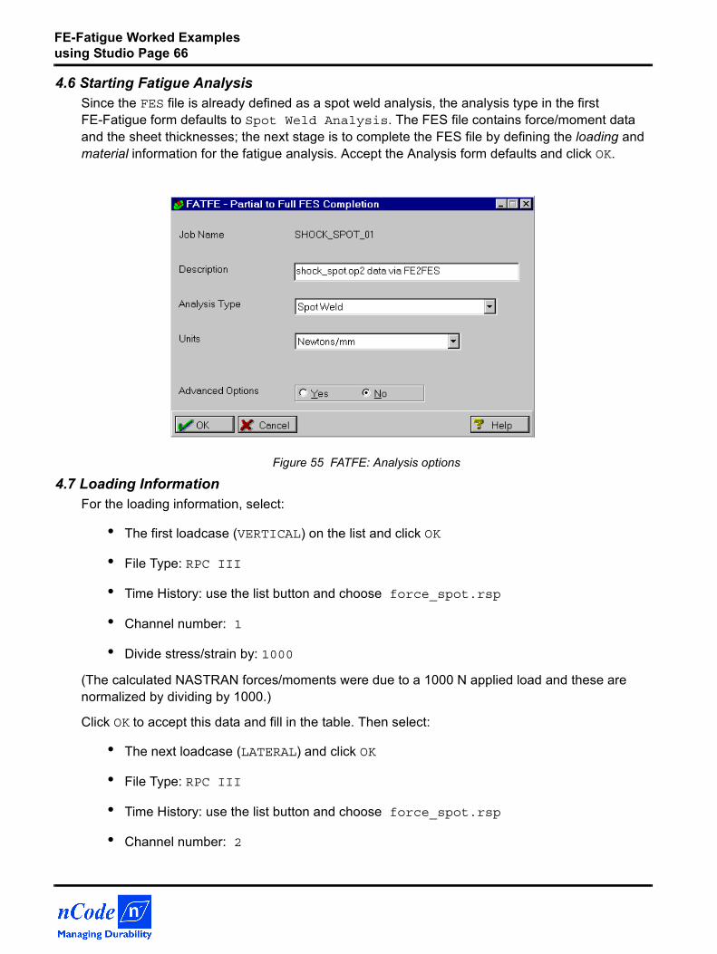
4.6 Starting Fatigue AnalysisSince the FES file is already defined as a spot weld analysis, the analysis type in the first FE-Fatigue form defaults to Spot Weld Analysis. The FES file contains force/moment data and the sheet thicknesses; the next stage is to complete the FES file by defining the loading and material information for the fatigue analysis. Accept the Analysis form defaults and click OK.
Figure 55 FATFE: Analysis options
4.7 Loading InformationFor the loading information, select:
• The first loadcase (VERTICAL) on the list and click OK
• File Type: RPC III
• Time History: use the list button and choose force_spot.rsp
• Channel number: 1
• Divide stress/strain by: 1000
(The calculated NASTRAN forces/moments were due to a 1000 N applied load and these are normalized by dividing by 1000.)
Click OK to accept this data and fill in the table. Then select:
• The next loadcase (LATERAL) and click OK
• File Type: RPC III
• Time History: use the list button and choose force_spot.rsp
• Channel number: 2
FE-Fatigue Worked Examples using Studio Page 67
• Divide stress/strain by: 1000
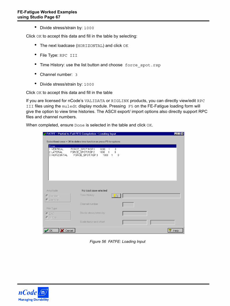
Click OK to accept this data and fill in the table by selecting:
• The next loadcase (HORIZONTAL) and click OK
• File Type: RPC III
• Time History: use the list button and choose force_spot.rsp
• Channel number: 3
• Divide stress/strain by: 1000
Click OK to accept this data and fill in the table
If you are licensed for nCode’s VALIDATA or RIGLINK products, you can directly view/edit RPCIII files using the muledt display module. Pressing F5 on the FE-Fatigue loading form will give the option to view time histories. The ASCII export/ import options also directly support RPC files and channel numbers.
When completed, ensure Done is selected in the table and click OK.
Figure 56 FATFE: Loading Input
FE-Fatigue Worked Examples using Studio Page 68
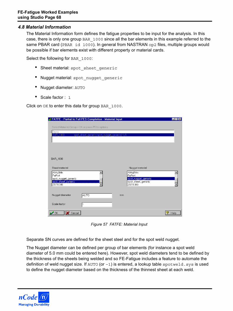
4.8 Material InformationThe Material Information form defines the fatigue properties to be input for the analysis. In this case, there is only one group BAR_1000 since all the bar elements in this example referred to the same PBAR card (PBAR id 1000). In general from NASTRAN op2 files, multiple groups would be possible if bar elements exist with different property or material cards.
Select the following for BAR_1000:
• Sheet material: spot_sheet_generic
• Nugget material: spot_nugget_generic
• Nugget diameter: AUTO
• Scale factor : 1
Click on OK to enter this data for group BAR_1000.
Figure 57 FATFE: Material Input
Separate SN curves are defined for the sheet steel and for the spot weld nugget.
The Nugget diameter can be defined per group of bar elements (for instance a spot weld diameter of 5.0 mm could be entered here). However, spot weld diameters tend to be defined by the thickness of the sheets being welded and so FE-Fatigue includes a feature to automate the definition of weld nugget size. If AUTO (or –1) is entered, a lookup table spotweld.sys is used to define the nugget diameter based on the thickness of the thinnest sheet at each weld.
FE-Fatigue Worked Examples using Studio Page 69
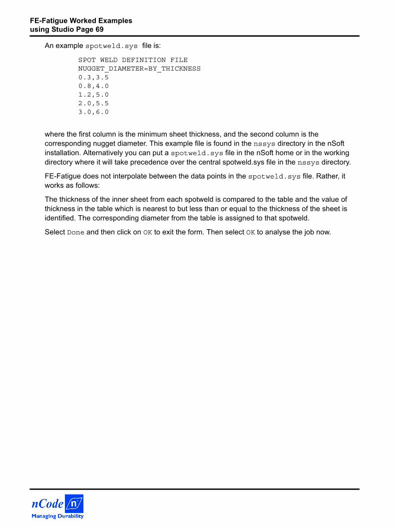
An example spotweld.sys file is:
SPOT WELD DEFINITION FILENUGGET_DIAMETER=BY_THICKNESS0.3,3.50.8,4.01.2,5.02.0,5.53.0,6.0
where the first column is the minimum sheet thickness, and the second column is the corresponding nugget diameter. This example file is found in the nssys directory in the nSoft installation. Alternatively you can put a spotweld.sys file in the nSoft home or in the working directory where it will take precedence over the central spotweld.sys file in the nssys directory.
FE-Fatigue does not interpolate between the data points in the spotweld.sys file. Rather, it works as follows:
The thickness of the inner sheet from each spotweld is compared to the table and the value of thickness in the table which is nearest to but less than or equal to the thickness of the sheet is identified. The corresponding diameter from the table is assigned to that spotweld.
Select Done and then click on OK to exit the form. Then select OK to analyse the job now.
FE-Fatigue Worked Examples using Studio Page 70
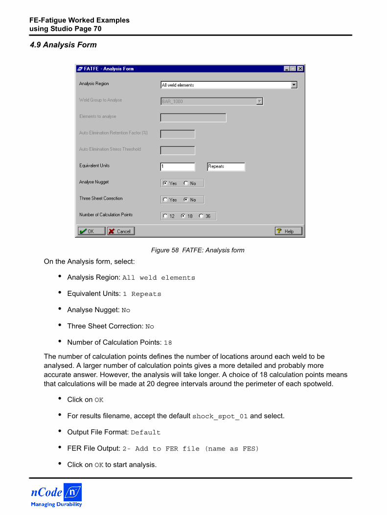
4.9 Analysis Form
Figure 58 FATFE: Analysis form
On the Analysis form, select:
• Analysis Region: All weld elements
• Equivalent Units: 1 Repeats
• Analyse Nugget: No
• Three Sheet Correction: No
• Number of Calculation Points: 18
The number of calculation points defines the number of locations around each weld to be analysed. A larger number of calculation points gives a more detailed and probably more accurate answer. However, the analysis will take longer. A choice of 18 calculation points means that calculations will be made at 20 degree intervals around the perimeter of each spotweld.
• Click on OK
• For results filename, accept the default shock_spot_01 and select.
• Output File Format: Default
• FER File Output: 2- Add to FER file (name as FES)
• Click on OK to start analysis.
FE-Fatigue Worked Examples using Studio Page 71
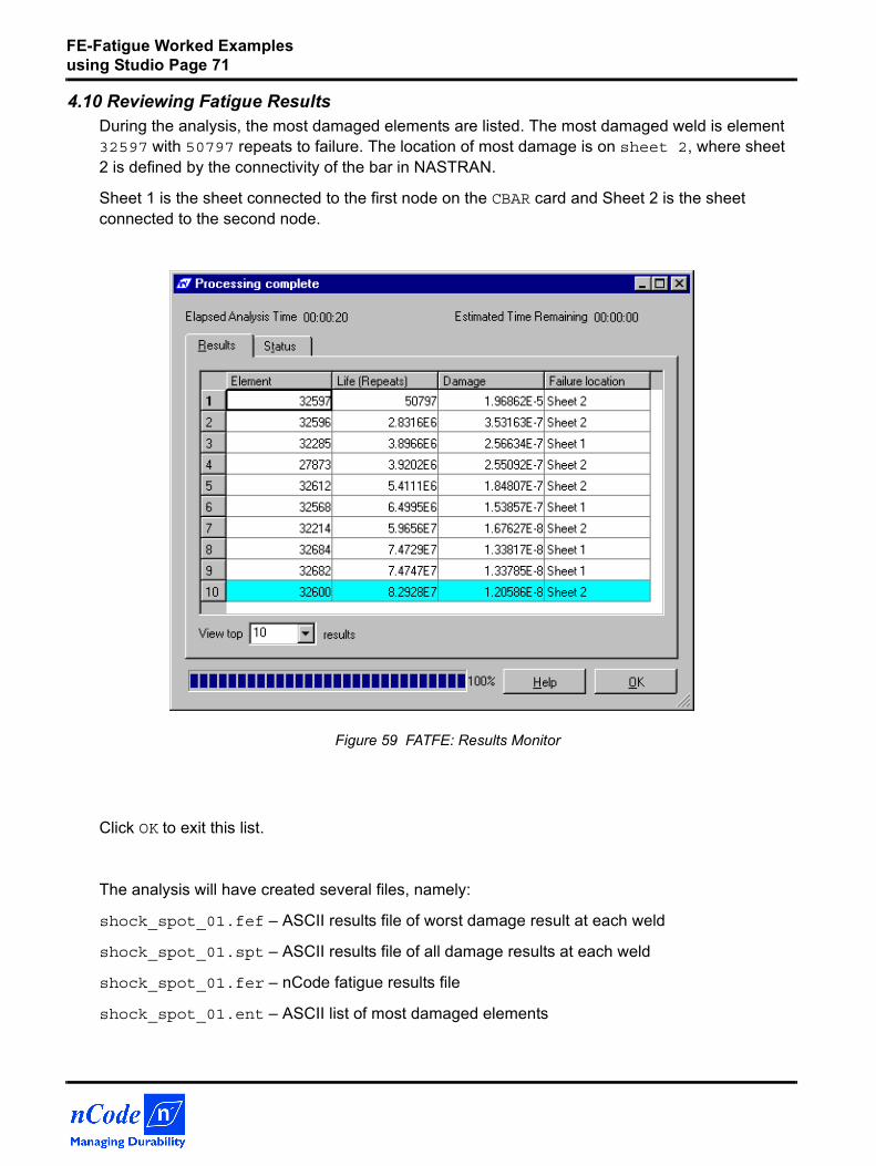
4.10 Reviewing Fatigue ResultsDuring the analysis, the most damaged elements are listed. The most damaged weld is element 32597 with 50797 repeats to failure. The location of most damage is on sheet 2, where sheet 2 is defined by the connectivity of the bar in NASTRAN.
Sheet 1 is the sheet connected to the first node on the CBAR card and Sheet 2 is the sheet connected to the second node.
Figure 59 FATFE: Results Monitor
Click OK to exit this list.
The analysis will have created several files, namely:
shock_spot_01.fef – ASCII results file of worst damage result at each weld
shock_spot_01.spt – ASCII results file of all damage results at each weld
shock_spot_01.fer – nCode fatigue results file
shock_spot_01.ent – ASCII list of most damaged elements

FE-Fatigue Worked Examples using Studio Page 72
For further information on the results, the Utilities menu provides several options including:
• Results Listing, which gives a spreadsheet summary of the shock_spot_01.fef file using fatres.
• Node/Element options which enable:– Time history extraction of stress at the most damaged locations around the weld. – Full results listing which gives results on a per angle basis for a weld (.spt file).– Polar plot to graphically view the results on an angle basis for a weld.
Investigate these options and create a polar plot of damage around the worst case weld element 32597.
FE-Fatigue Worked Examples using Studio Page 73
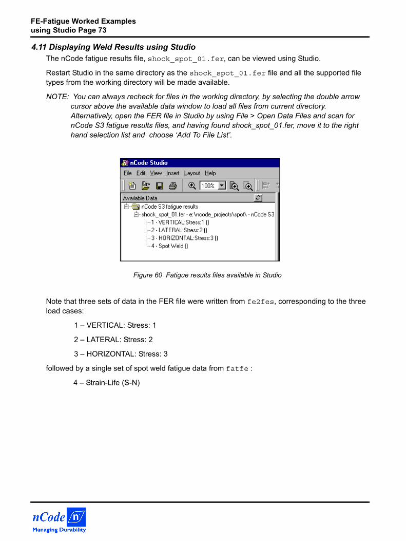
4.11 Displaying Weld Results using StudioThe nCode fatigue results file, shock_spot_01.fer, can be viewed using Studio.
Restart Studio in the same directory as the shock_spot_01.fer file and all the supported file types from the working directory will be made available.
NOTE: You can always recheck for files in the working directory, by selecting the double arrow cursor above the available data window to load all files from current directory. Alternatively, open the FER file in Studio by using File > Open Data Files and scan for nCode S3 fatigue results files, and having found shock_spot_01.fer, move it to the right hand selection list and choose ‘Add To File List’.
Figure 60 Fatigue results files available in Studio
Note that three sets of data in the FER file were written from fe2fes, corresponding to the three load cases:
1 – VERTICAL: Stress: 1
2 – LATERAL: Stress: 2
3 – HORIZONTAL: Stress: 3
followed by a single set of spot weld fatigue data from fatfe :
4 – Strain-Life (S-N)
FE-Fatigue Worked Examples using Studio Page 74
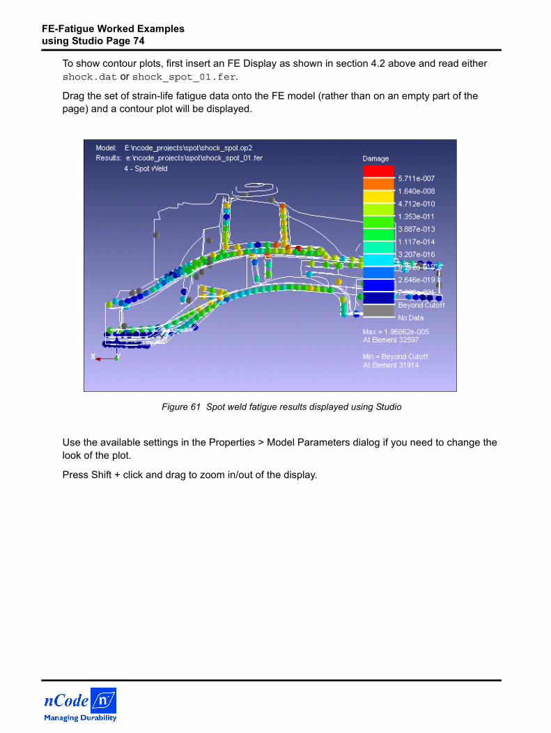
To show contour plots, first insert an FE Display as shown in section 4.2 above and read either shock.dat or shock_spot_01.fer.
Drag the set of strain-life fatigue data onto the FE model (rather than on an empty part of the page) and a contour plot will be displayed.
Figure 61 Spot weld fatigue results displayed using Studio
Use the available settings in the Properties > Model Parameters dialog if you need to change the look of the plot.
Press Shift + click and drag to zoom in/out of the display.
FE-Fatigue Worked Examples using Studio Page 75
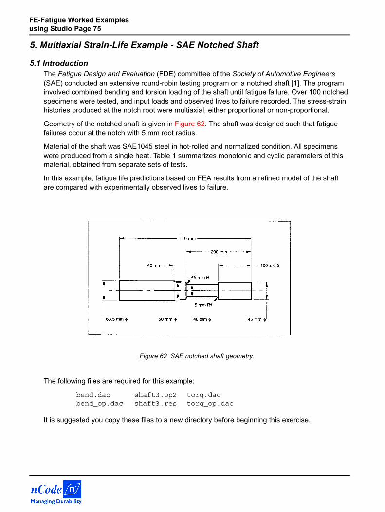
5. Multiaxial Strain-Life Example - SAE Notched Shaft
5.1 IntroductionThe Fatigue Design and Evaluation (FDE) committee of the Society of Automotive Engineers (SAE) conducted an extensive round-robin testing program on a notched shaft [1]. The program involved combined bending and torsion loading of the shaft until fatigue failure. Over 100 notched specimens were tested, and input loads and observed lives to failure recorded. The stress-strain histories produced at the notch root were multiaxial, either proportional or non-proportional.
Geometry of the notched shaft is given in Figure 62. The shaft was designed such that fatigue failures occur at the notch with 5 mm root radius.
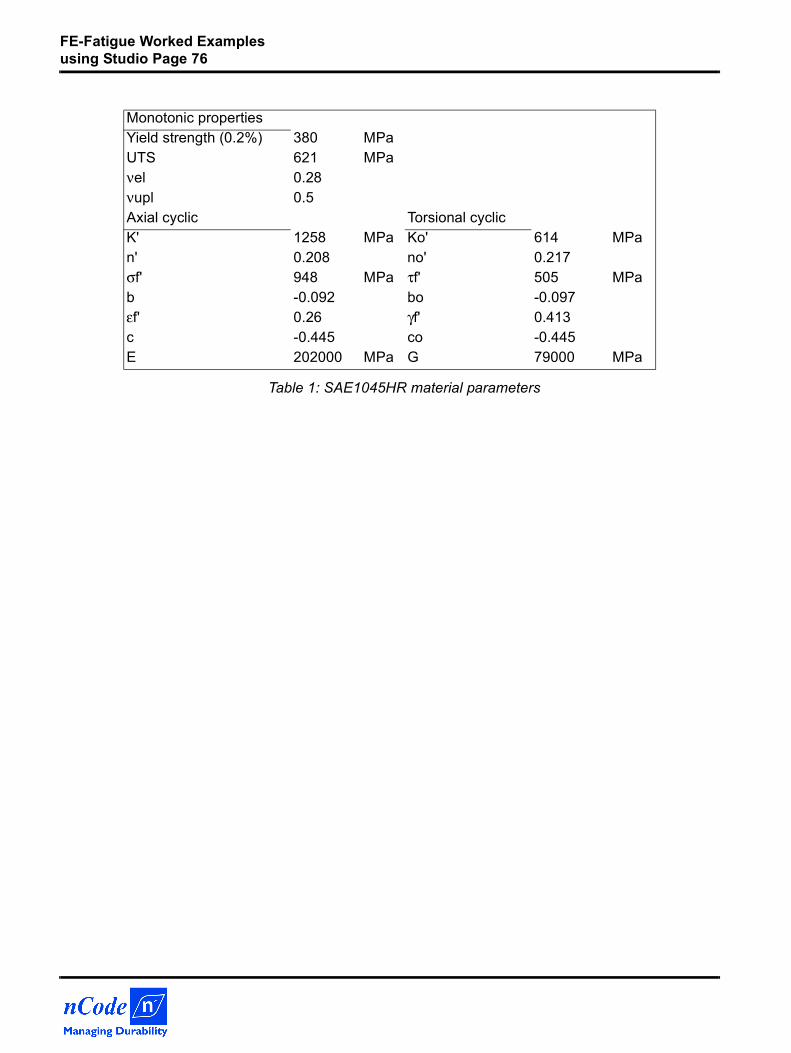
Material of the shaft was SAE1045 steel in hot-rolled and normalized condition. All specimens were produced from a single heat. Table 1 summarizes monotonic and cyclic parameters of this material, obtained from separate sets of tests.
In this example, fatigue life predictions based on FEA results from a refined model of the shaft are compared with experimentally observed lives to failure.
Figure 62 SAE notched shaft geometry.
The following files are required for this example:
bend.dac shaft3.op2 torq.dacbend_op.dac shaft3.res torq_op.dac
It is suggested you copy these files to a new directory before beginning this exercise.
FE-Fatigue Worked Examples using Studio Page 76
Table 1: SAE1045HR material parameters
Monotonic propertiesYield strength (0.2%) 380 MPaUTS 621 MPaνel 0.28νupl 0.5Axial cyclic Torsional cyclicK' 1258 MPa Ko' 614 MPan' 0.208 no' 0.217σf' 948 MPa τf' 505 MPab -0.092 bo -0.097εf' 0.26 γf' 0.413c -0.445 co -0.445E 202000 MPa G 79000 MPa
FE-Fatigue Worked Examples using Studio Page 77
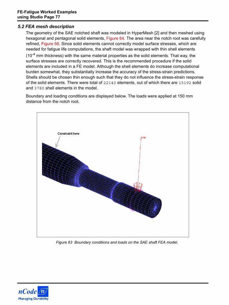
5.2 FEA mesh descriptionThe geometry of the SAE notched shaft was modeled in HyperMesh [2] and then meshed using hexagonal and pentagonal solid elements, Figure 64. The area near the notch root was carefully refined, Figure 66. Since solid elements cannot correctly model surface stresses, which are needed for fatigue life computations, the shaft model was wrapped with thin shell elements (10-4 mm thickness) with the same material properties as the solid elements. That way, the surface stresses are correctly recovered. This is the recommended procedure if the solid elements are included in a FE model. Although the shell elements do increase computational burden somewhat, they substantially increase the accuracy of the stress-strain predictions. Shells should be chosen thin enough such that they do not influence the stress-strain response of the solid elements. There were total of 22140 elements, out of which there are 15192 solid and 3780 shell elements in the model.
Boundary and loading conditions are displayed below. The loads were applied at 150 mm distance from the notch root.
Figure 63 Boundary conditions and loads on the SAE shaft FEA model.
FE-Fatigue Worked Examples using Studio Page 78
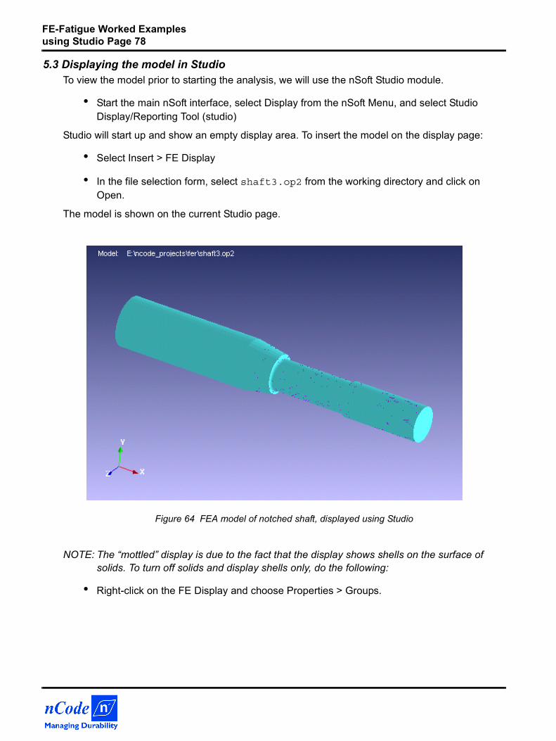
5.3 Displaying the model in StudioTo view the model prior to starting the analysis, we will use the nSoft Studio module.
• Start the main nSoft interface, select Display from the nSoft Menu, and select Studio Display/Reporting Tool (studio)
Studio will start up and show an empty display area. To insert the model on the display page:
• Select Insert > FE Display
• In the file selection form, select shaft3.op2 from the working directory and click on Open.
The model is shown on the current Studio page.
Figure 64 FEA model of notched shaft, displayed using Studio
NOTE: The “mottled” display is due to the fact that the display shows shells on the surface of solids. To turn off solids and display shells only, do the following:
• Right-click on the FE Display and choose Properties > Groups.
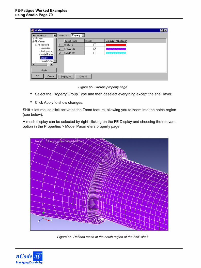
FE-Fatigue Worked Examples using Studio Page 79
Figure 65 Groups property page
• Select the Property Group Type and then deselect everything except the shell layer.
• Click Apply to show changes.
Shift + left mouse click activates the Zoom feature, allowing you to zoom into the notch region (see below).
A mesh display can be selected by right-clicking on the FE Display and choosing the relevant option in the Properties > Model Parameters property page.
Figure 66 Refined mesh at the notch region of the SAE shaft
FE-Fatigue Worked Examples using Studio Page 80
5.4 Linear static FEA solutionIn this case, the bending force and torque were applied as two separate static sub-cases to the FEA model, and solved using NASTRAN [3]. The magnitudes of the bending force and torque were 1000 N and 1000 Nmm, respectively. The static sub-cases will be combined within FE-Fatigue with actual bending and torque loading histories using the principle of superposition to produce stress histories for all or selected nodes of the model.
When using multiaxial EN analysis with linear static stress superposition, FE-Fatigue corrects linear elastic stress-strain results to elastic-plastic results using multiaxial Neuber correction with Mroz-Garud kinematic plasticity model.
FE-Fatigue Worked Examples using Studio Page 81
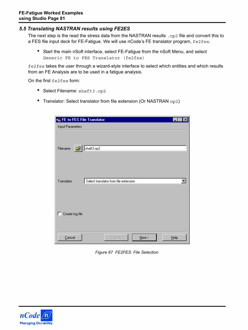
5.5 Translating NASTRAN results using FE2ESThe next step is the read the stress data from the NASTRAN results .op2 file and convert this to a FES file input deck for FE-Fatigue. We will use nCode’s FE translator program, fe2fes.
• Start the main nSoft interface, select FE-Fatigue from the nSoft Menu, and select Generic FE to FES Translator (fe2fes)
fe2fes takes the user through a wizard-style interface to select which entities and which results from an FE Analysis are to be used in a fatigue analysis.
On the first fe2fes form:
• Select Filename: shaft3.op2
• Translator: Select translator from file extension (Or NASTRAN op2)
Figure 67 FE2FES: File Selection
FE-Fatigue Worked Examples using Studio Page 82
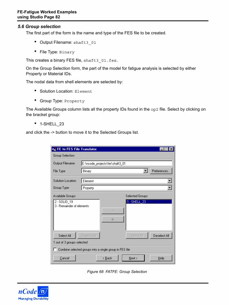
5.6 Group selectionThe first part of the form is the name and type of the FES file to be created.
• Output Filename: shaft3_01
• File Type: Binary
This creates a binary FES file, shaft3_01.fes.
On the Group Selection form, the part of the model for fatigue analysis is selected by either Property or Material IDs.
The nodal data from shell elements are selected by:
• Solution Location: Element
• Group Type: Property
The Available Groups column lists all the property IDs found in the op2 file. Select by clicking on the bracket group:
• 1-SHELL_23
and click the -> button to move it to the Selected Groups list.
Figure 68 FATFE: Group Selection
FE-Fatigue Worked Examples using Studio Page 83
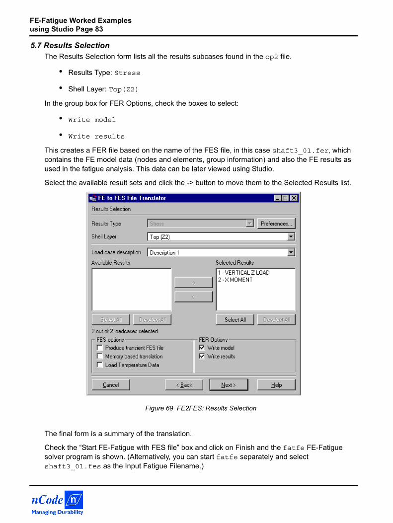
5.7 Results SelectionThe Results Selection form lists all the results subcases found in the op2 file.
• Results Type: Stress
• Shell Layer: Top(Z2)
In the group box for FER Options, check the boxes to select:
• Write model
• Write results
This creates a FER file based on the name of the FES file, in this case shaft3_01.fer, which contains the FE model data (nodes and elements, group information) and also the FE results as used in the fatigue analysis. This data can be later viewed using Studio.
Select the available result sets and click the -> button to move them to the Selected Results list.
Figure 69 FE2FES: Results Selection
The final form is a summary of the translation.
Check the “Start FE-Fatigue with FES file” box and click on Finish and the fatfe FE-Fatigue solver program is shown. (Alternatively, you can start fatfe separately and select shaft3_01.fes as the Input Fatigue Filename.)
FE-Fatigue Worked Examples using Studio Page 84
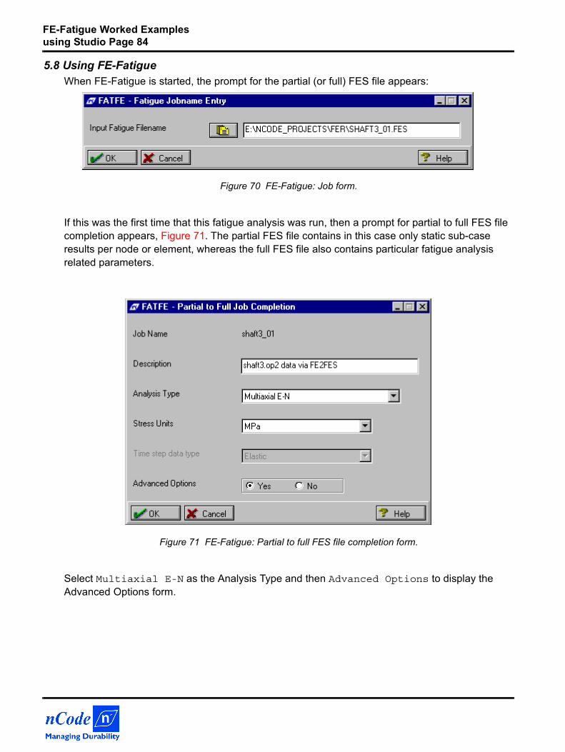
5.8 Using FE-FatigueWhen FE-Fatigue is started, the prompt for the partial (or full) FES file appears:
Figure 70 FE-Fatigue: Job form.
If this was the first time that this fatigue analysis was run, then a prompt for partial to full FES file completion appears, Figure 71. The partial FES file contains in this case only static sub-case results per node or element, whereas the full FES file also contains particular fatigue analysis related parameters.
Figure 71 FE-Fatigue: Partial to full FES file completion form.
Select Multiaxial E-N as the Analysis Type and then Advanced Options to display the Advanced Options form.
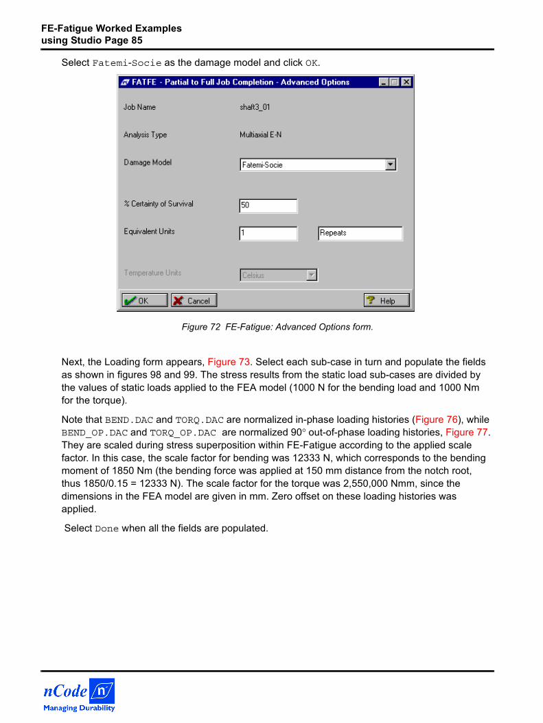
FE-Fatigue Worked Examples using Studio Page 85
Select Fatemi-Socie as the damage model and click OK.
Figure 72 FE-Fatigue: Advanced Options form.
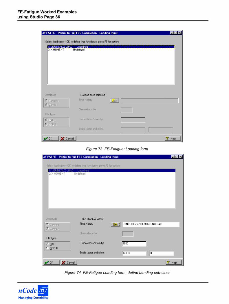
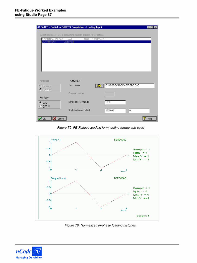
Next, the Loading form appears, Figure 73. Select each sub-case in turn and populate the fields as shown in figures 98 and 99. The stress results from the static load sub-cases are divided by the values of static loads applied to the FEA model (1000 N for the bending load and 1000 Nm for the torque).
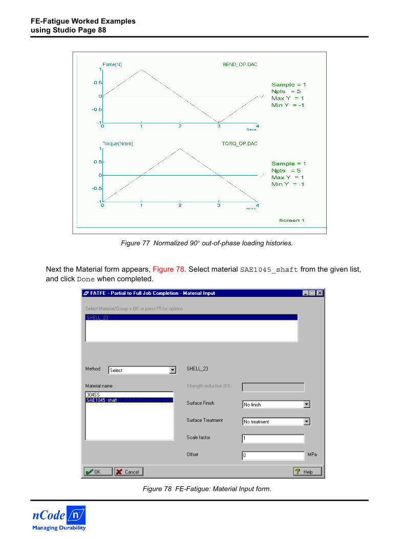
Note that BEND.DAC and TORQ.DAC are normalized in-phase loading histories (Figure 76), while BEND_OP.DAC and TORQ_OP.DAC are normalized 90° out-of-phase loading histories, Figure 77. They are scaled during stress superposition within FE-Fatigue according to the applied scale factor. In this case, the scale factor for bending was 12333 N, which corresponds to the bending moment of 1850 Nm (the bending force was applied at 150 mm distance from the notch root, thus 1850/0.15 = 12333 N). The scale factor for the torque was 2,550,000 Nmm, since the dimensions in the FEA model are given in mm. Zero offset on these loading histories was applied.
Select Done when all the fields are populated.
FE-Fatigue Worked Examples using Studio Page 86
Figure 73 FE-Fatigue: Loading form
Figure 74 FE-Fatigue Loading form: define bending sub-case
FE-Fatigue Worked Examples using Studio Page 87
Figure 75 FE-Fatigue loading form: define torque sub-case
Figure 76 Normalized in-phase loading histories.
FE-Fatigue Worked Examples using Studio Page 88
Figure 77 Normalized 90° out-of-phase loading histories.
Next the Material form appears, Figure 78. Select material SAE1045_shaft from the given list, and click Done when completed.
Figure 78 FE-Fatigue: Material Input form.
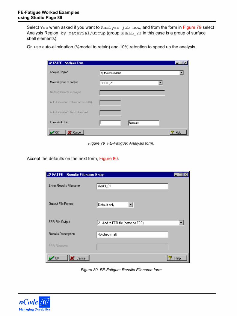
FE-Fatigue Worked Examples using Studio Page 89
Select Yes when asked if you want to Analyze job now, and from the form in Figure 79 select Analysis Region by Material/Group (group SHELL_23 in this case is a group of surface shell elements).
Or, use auto-elimination (%model to retain) and 10% retention to speed up the analysis.
Figure 79 FE-Fatigue: Analysis form.
Accept the defaults on the next form, Figure 80.
Figure 80 FE-Fatigue: Results Filename form
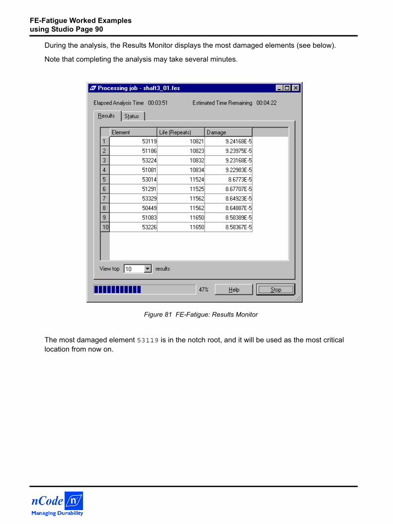
FE-Fatigue Worked Examples using Studio Page 90
During the analysis, the Results Monitor displays the most damaged elements (see below).
Note that completing the analysis may take several minutes.
Figure 81 FE-Fatigue: Results Monitor
The most damaged element 53119 is in the notch root, and it will be used as the most critical location from now on.
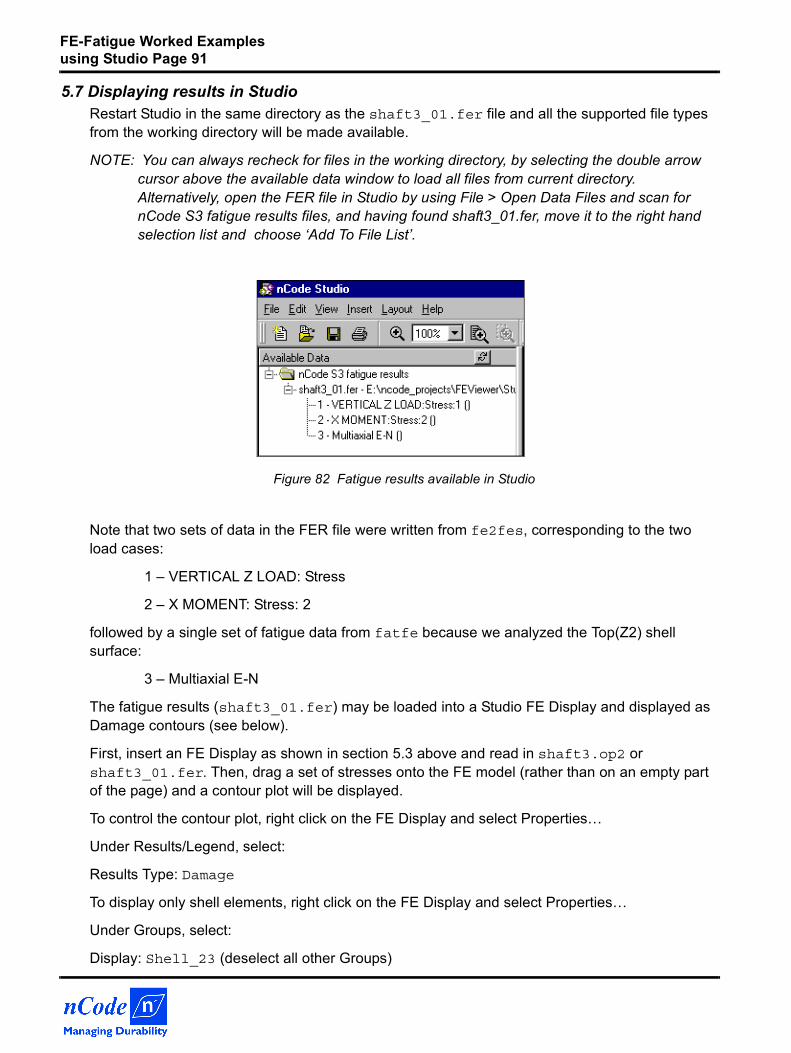
FE-Fatigue Worked Examples using Studio Page 91
5.7 Displaying results in StudioRestart Studio in the same directory as the shaft3_01.fer file and all the supported file types from the working directory will be made available.
NOTE: You can always recheck for files in the working directory, by selecting the double arrow cursor above the available data window to load all files from current directory. Alternatively, open the FER file in Studio by using File > Open Data Files and scan for nCode S3 fatigue results files, and having found shaft3_01.fer, move it to the right hand selection list and choose ‘Add To File List’.
Figure 82 Fatigue results available in Studio
Note that two sets of data in the FER file were written from fe2fes, corresponding to the two load cases:
1 – VERTICAL Z LOAD: Stress
2 – X MOMENT: Stress: 2
followed by a single set of fatigue data from fatfe because we analyzed the Top(Z2) shell surface:
3 – Multiaxial E-N
The fatigue results (shaft3_01.fer) may be loaded into a Studio FE Display and displayed as Damage contours (see below).
First, insert an FE Display as shown in section 5.3 above and read in shaft3.op2 or shaft3_01.fer. Then, drag a set of stresses onto the FE model (rather than on an empty part of the page) and a contour plot will be displayed.
To control the contour plot, right click on the FE Display and select Properties…
Under Results/Legend, select:
Results Type: Damage
To display only shell elements, right click on the FE Display and select Properties…
Under Groups, select:
Display: Shell_23 (deselect all other Groups)
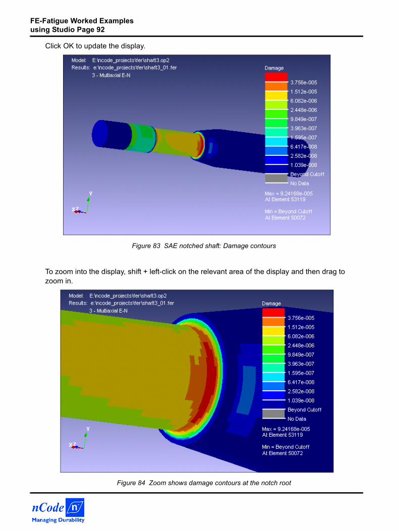
FE-Fatigue Worked Examples using Studio Page 92
Click OK to update the display.
Figure 83 SAE notched shaft: Damage contours
To zoom into the display, shift + left-click on the relevant area of the display and then drag to zoom in.
Figure 84 Zoom shows damage contours at the notch root
FE-Fatigue Worked Examples using Studio Page 93
5.8 Comparison with experimental dataNow that the critical location is known, a variety of different fatigue analyses can be performed on it, either by keeping the same loads and changing the damage model (Edit Job/EditAnalysis options), or keeping the same damage model and changing the loads by applying different scaling factors to them (Edit Job/Edit Load Input). Two damage models were employed in this example: Fatemi-Socie and Wang-Brown [4].
Table 2 lists experimental results and predictions for a variety of in-phase loadings, while table 3 lists the same for a variety of 90° out-of-phase loadings. Note that the loading functions for the out-of-phase loading were changed from BEND.DAC and TORQ.DAC to BEND_OP.DAC and TORQ_OP.DAC, respectively.
Experimentation of this type can be performed on a reduced set of nodes by selection of the analysis region to be specified nodes rather than by Group. Either a single node ID, e.g. 53119, can be entered directly or the group of nodes specified in the file SHAFT3.ENT from the previous run can be used by copying SHAFT3.ENT to another name, e.g. SHAFT3.SAV and specifying @SHAFT3.SAV in the node/element input field. This will greatly reduce calculation time.
It should be emphasized that the critical location and the associated lives to failure change slightly with the changing levels of non-proportionality. Also, the predicted lives to failure change with both increasing number of points in the loading histories and with changing the waveforms of the histories. Several different cases have been tested, with number of points in the histories ranging from 5 to 500, and with waveforms of the histories ranging from triangular, to trapezoidal, to sine waves. Overall, the differences in life predictions between the tested cases were rather small (within 15% on life for either the Fatemi-Socie or the Wang-Brown method). The analyses here are presented for one critical element only (element 53119), with triangular loading histories, and with only peaks and valleys representing the time histories (thus only 4 to 5 points in the histories).
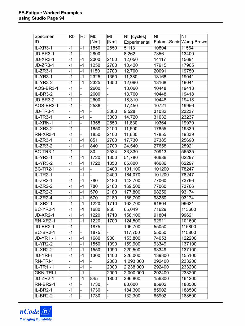
FE-Fatigue Worked Examples using Studio Page 94
Specimen ID
Rb Rt Mb [Nm]
Mt [Nm]
Nf [cycles]Experimental
Nf Fatemi-Socie
Nf Wang-Brown
IL-XR3-1 -1 -1 1850 2550 5,113 10804 11564JD-BR3-1 -1 - 2800 - 8,262 7356 13400JD-XR3-1 -1 -1 2000 2100 12,050 14117 15691JD-ZR3-1 -1 -1 1250 2700 10,420 17915 17965IL-ZR3-1 -1 -1 1150 2700 12,700 20091 19750IL-YR3-1 -1 -1 2325 1350 11,380 13168 19041IL-YR3-2 -1 -1 2325 1350 12,090 13168 19041AOS-BR3-1 -1 - 2600 - 13,060 10448 19418IL-BR3-2 -1 - 2600 - 13,760 10448 19418JD-BR3-2 -1 - 2600 - 18,310 10448 19418AOS-BR3-1 -1 - 2586 - 17,450 10721 19956JD-TR3-1 - -1 - 3000 9,528 31032 23237IL-TR3-1 - -1 - 3000 14,720 31032 23237IL-XRN- I -1 - 1355 2550 11,630 19364 19970IL-XR3-2 -1 - 1850 2100 11,500 17855 19339RN-XR3-1 -1 - 1850 2100 11,630 17855 19339IL-ZR3-1 -1 -1 851 2700 17,730 27385 25690IL-ZR3-2 -1 -1 840 2700 24,540 27658 25921BC-TR3-1 -1 - 80 2534 33,330 70913 56535IL-YR3-1 -1 -1 1720 1350 51,780 46686 62297IL-YR3-2 -1 -1 1720 1350 65,800 46686 62297BC-TR2-1 - -1 - 2400 101,100 101200 78247IL-TR2-1 - -1 - 2400 164,070 101200 78247IL-ZR2-1 -1 -1 780 2180 142,700 77060 73766IL-ZR2-2 -1 -1 780 2180 169,500 77060 73766IL-ZR2-3 -1 -1 570 2180 177,800 98250 93174IL-ZR2-4 -1 -1 570 2180 186,700 98250 93174IL-XR2-1 -1 -1 1220 1710 163,700 91804 99621BC-YR2-1 -1 -1 1680 960 65,049 71629 113600JD-XR2-1 -1 -1 1220 1710 158,100 91804 99621RN-XR2-1 -1 -1 1220 1700 124,500 92911 101600JD-BR2-1 -1 - 1875 - 106,700 55050 115800BC-BR2-1 -1 - 1875 - 117,700 55050 115800JD-YR I - I -1 -1 1680 900 153,800 74053 122200IL-YR2-2 -1 -1 1550 1090 159,900 93349 137100IL-XR2-2 -1 -1 1550 1090 220,500 93349 137100JD-YRI-I -1 -1 1300 1400 226,000 139300 155100RN-TRI-1 - -1 - 2000 1,293,000 292400 233200IL-TR1 - 1 - -1 - 2000 2,238,000 292400 233200GKN-TRI-I - -1 - 2000 2,000,000 292400 233200JD-ZR2-1 -1 -1 845 1800 396,800 156800 164200RN-BR2-1 -1 - 1730 - 83,600 85902 188500IL-BR2-1 -1 - 1730 - 184,300 85902 188500IL-BR2-2 -1 - 1730 - 132,300 85902 188500
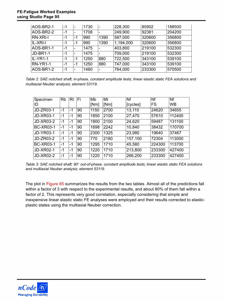
FE-Fatigue Worked Examples using Studio Page 95
Table 2: SAE notched shaft; in-phase, constant amplitude tests; linear elastic static FEA solutions and multiaxial Neuber analysis; element 53119.
Table 3: SAE notched shaft; 90° out-of-phase, constant amplitude tests; linear elastic static FEA solutions and multiaxial Neuber analysis; element 53119.
The plot in Figure 85 summarizes the results from the two tables. Almost all of the predictions fall within a factor of 3 with respect to the experimental results, and about 80% of them fall within a factor of 2. This represents very good correlation, especially considering that simple and inexpensive linear elastic static FE analyses were employed and their results corrected to elastic-plastic states using the multiaxial Neuber correction.
AOS-BR2-1 -1 - 1730 - 228,300 85902 188500AOS-BR2-2 -1 - 1708 - 249,900 92381 204200RN-XRI-l -1 -1 990 1390 587,000 320600 356800IL-XRI-l -1 -1 990 1390 1,194,000 320600 356800AOS-BR1-1 -1 - 1475 - 403,800 219100 532300JD-BR1-1 -1 - 1475 - 709,000 219100 532300IL-YR1-1 -1 -1 1250 880 722,500 343100 539100RN-YR1-1 -1 -1 1250 880 747,000 343100 539100AOS-BR1-2 -1 - 1460 - 764,000 233300 570500
Specimen ID
Rb Rt Fi Mb [Nm]
Mt [Nm]
Nf [cycles]
Nf FS
Nf WB
JD-ZR03-1 -1 -1 90 1150 2700 13,110 24620 34655JD-XR03-1 -1 -1 90 1850 2100 27,470 57610 112400JD-XR03-2 -1 -1 90 1800 2100 24,620 59487 131100BC-XR03-1 -1 -1 90 1698 2242 10,840 38432 170700JD-YR03-1 -1 -1 90 2300 1325 23,980 19640 37467JD-ZR03-2 -1 -1 90 770 2180 157,100 72304 113000BC-XR03-1 -1 -1 90 1295 1710 45,580 224300 113700JD-XR02-1 -1 -1 90 1220 1710 213,800 233300 427400JD-XR02-2 -1 -1 90 1220 1710 266,200 233300 427400
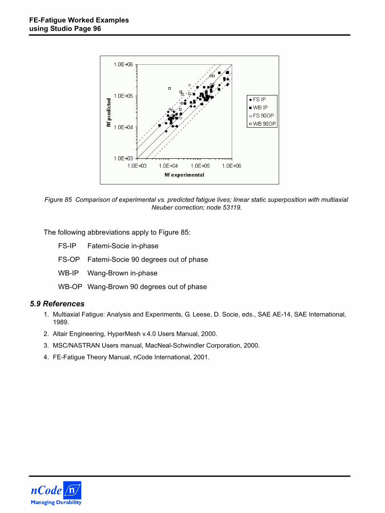
FE-Fatigue Worked Examples using Studio Page 96
Figure 85 Comparison of experimental vs. predicted fatigue lives; linear static superposition with multiaxial Neuber correction; node 53119.
The following abbreviations apply to Figure 85:
FS-IP Fatemi-Socie in-phase
FS-OP Fatemi-Socie 90 degrees out of phase
WB-IP Wang-Brown in-phase
WB-OP Wang-Brown 90 degrees out of phase
5.9 References1. Multiaxial Fatigue: Analysis and Experiments, G. Leese, D. Socie, eds., SAE AE-14, SAE International,
1989.
2. Altair Engineering, HyperMesh v.4.0 Users Manual, 2000.
3. MSC/NASTRAN Users manual, MacNeal-Schwindler Corporation, 2000.
4. FE-Fatigue Theory Manual, nCode International, 2001.