Embed Size (px)
Citation preview

Arab J Sci Eng (2017) 42:1103–1116DOI 10.1007/s13369-016-2316-y
RESEARCH ARTICLE - CIVIL ENGINEERING
FE Model of the Fatih Sultan Mehmet Suspension BridgeUsing Thin Shell Finite Elements
S. A. Kilic1 · H. J. Raatschen2 · B. Körfgen3 · N. M. Apaydin4 · A. Astaneh-Asl5
Received: 12 December 2015 / Accepted: 20 September 2016 / Published online: 1 October 2016© The Author(s) 2016. This article is published with open access at Springerlink.com
Abstract This paper presents the results of an eigenvalueanalysis of the Fatih Sultan Mehmet Bridge. A high-resolution finite element model was created directly fromthe available design documents. All physical properties ofthe structural components were included in detail, so no cal-ibration to the measured data was necessary. The deck andtowers were modeled with shell elements. A nonlinear sta-tic analysis was performed before the eigenvalue calculation.The calculated natural frequencies and corresponding modeshapes showed good agreement with the available measuredambient vibration data. The calculation of the effectivemodalmass showed that ninemodes had single contributions higher
B S. A. [email protected]
H. J. [email protected]
B. Kö[email protected]
N. M. [email protected]
1 Department of Civil Engineering, Bogazici University, 34342Bebek, Istanbul, Turkey
2 Department of Mechanical Engineering, FH AachenUniversity of Applied Sciences, 52064 Aachen, Germany
3 Forschungszentrum Jülich GmbH, Institute for AdvancedSimulation, Jülich Supercomputing Centre, 52425 Jülich,Germany
4 Turkish Directorate of Highways, District 1, 34408Kagithane, Istanbul, Turkey
5 Department of Civil and Environmental Engineering,University of California at Berkeley, Berkeley, CA 94720,USA
than 5% of the total mass. They were in a frequency rangeup to 1.2Hz. The comparison of the results for the torsionalmodes especially demonstrated the advantage of using thinshell finite elements over the beam modeling approach.
Keywords Suspension bridge · 3D nonlinear finite elementmodel · Thin shell finite elements · Natural frequency ·Effective modal mass
1 Introduction
Analyzing the dynamic response of long-span suspensionbridges is a challenging task for bridge engineers. A greatmajority of the studies available in the literature employedbeam elements to model the main, back-stay, and hangercables and the towers and orthotropic deck structure.
The input parameters for the beam elements consistof the equivalent overall cross-sectional properties of theorthotropic deck and towers, such as the cross-sectionalarea, effective shear area, moments of inertia, and torsionalconstant. While the moments of inertia for bending can beapproximated with a reasonable level of accuracy, determin-ing the torsional constants for the towers and orthotropic deckstructure with diaphragms is a difficult task. The orthotropicdeck and towers can be approximated by using beam ele-ments. Individual structural components such as the stiffenerbeams and diaphragms cannot be modeled directly by usingbeam elements.
The beam element models of suspension bridges requirefine-tuning of the input parameters in order to match theambient vibration test results. However, it is difficult toobtain matching results for the lateral, vertical, and tor-sional modes of vibration by using a limited set of equivalentoverall cross-sectional properties. The accuracy of the beam
123
1104 Arab J Sci Eng (2017) 42:1103–1116
models is reasonable for modes of vibration with lowerfrequencies and questionable for higher modes. In addi-tion, the effects of a localized stress concentration cannotbe modeled by using beam elements in advanced nonlineardynamic analyses. Therefore, beam element models of sus-pension bridges have been restricted to studies on the globalresponse.
The alternative approach proposed in this paper is to useshell elements in order to better represent the towers and deckstructure of suspension bridges. This procedure allows thebuilding of finite element (FE) models with fine resolutionsby explicitly modeling the individual structural componentsof the towers and deck structure. The use of a shell ele-ment model removes the burden of estimating the equivalentoverall cross-sectional properties of the orthotropic deck andtowers. Shell element models provide better accuracy thanbeam element models not only for lower-frequency modesbut also for the higher modes of vibration.
Brownjohn et al. [1,2] conducted ambient vibration testson the Fatih Sultan Mehmet Suspension Bridge to measurethe vertical, lateral, and torsional modes of the deck and tow-ers up to a frequency of 2 Hz. They employed auto powerspectrum methods to identify the modal frequencies. Theyconstructed numericalmodels employing beam elements andconcluded that the measured and computed values agreedwell at low frequencies [3]. However, they observed anincreasing divergence at higher frequencies. Abdel-Ghaffarand Stringfellow [4] investigated the dynamic response ofsuspension bridges and concluded that a relatively largenumber of modes are necessary to obtain a reasonable repre-sentation of the lateral response, which is similar to the casefor vertical response analysis.
Apaydin studied the dynamic response of the Fatih Sul-tan Mehmet Bridge and employed a three-dimensional FEmodel with beam elements [5,6]. The agreement between thefinite element results and measured ambient vibrations in theexperiment was better for the lateral and vertical modes thanfor the torsional modes because of the difficulty with repre-senting the orthotropic deck structure having diaphragms byusing beam elements.
Daniell and Macdonald [7] applied model updating tech-niques with systematic manual tuning to develop FE modelsof cable-stayed bridges. Their FE model employs shell ele-ments for the reinforced concrete slab and beam elementsfor the orthotropic steel box section deck. They pointed outthe difficulties of modeling the orthotropic deck with manyinternal components when using beam elements.
Zhang et al. [8] studied the ambient vibrations on suspen-sion bridges and compared themeasured data with the resultsof FE models that utilized a combination of beam and shellelements. They emphasized the contribution of the towers tothe overall response of the bridge and identified the towermodes up to a frequency of 7.7 Hz from the measured data.
In most of these studies, some of the bridge componentswere simplified. The orthotropic deck structure with inter-nal diaphragms was often modeled with beam elements. Thetowermotionwas sometimes neglected or approximatedwiththe use of beamelements that only approximately representedthe stiffness of the internal tower diaphragms and stiffenerbeams. The equivalent cross-sectional properties requiredfine-tuning in order to match the ambient vibration test mea-surements.
Few suspension bridge studies that employed shell ele-ments can be found in the open literature. Rahbari andBrownjohn built two FEmodels consisting of beam and shellelements for the Humber Bridge [9]. They compared thenumerical results with the available experimental data. Theymodeled the deck structure with equivalent plate elementsin the low-resolution model. They provided an alternativemodeling approach with equivalent box sections in the high-resolution model. They concluded that the low-resolutionmodel was inadequate in terms of matching the measuredmodal frequencies of the bridge and emphasized the needfor high-resolution models to conduct dynamic studies.
Most finite element models of suspension bridges havelow mesh resolutions and employ mainly beam elements.Karmakar et al. modeled the Vincent Thomas SuspensionBridge using shell elements only for the 165-mm-thick rein-forced concrete deck, and a combination of beam and trusselements for all other components of the structural sys-tem [10]. The FE model consisted of 4913 beam elementsand 6800 shell elements. They validated the finite elementmodel by comparing the computed eigenproperties of thebridge with the system identification results obtained usingambient vibration data. Duan et al. [11] provided a detailedFE model for the Tsing Ma Suspension Bridge. They com-pared the numerical results with the measured data from theambient vibrations tests. The FE model consisted of half amillion beam, shell, and hexahedral elements. They mod-eled the structural components of the deck in detail insteadof using beam elements with approximate cross-sectionalproperties. Rocker bearings of the bridge were incorporateddirectly into the FE model. They emphasized the need forFE models with high resolution in order to carry out healthmonitoring studies that require the identification of criticallocations and components.
In this study, shell elements were employed to model thegeometry and internal structural components of the towersand orthotropic bridge deck of the Fatih Sultan Mehmet(FSM) Bridge located in Istanbul, Turkey. Only the sus-pension, back-stay, and hanger cables were modeled withbeam elements. The modus operandi of the current studyavoided the need for fine-tuning the approximate cross-sectional properties. The dynamic analysis was preceded bya nonlinear static analysis that required the establishmentof the correct tensile forces in the cables and the converged
123
Arab J Sci Eng (2017) 42:1103–1116 1105
equilibrium geometry of the structure after the application ofthe dead and live loads.
The objective of this study was to build a high-resolutionFE model of the FSM Bridge. This FE model was appliedto calculating the eigenmodes of the FSM Bridge using thecommercial finite element software LS-DYNA [12] and wasvalidated by comparing the results, i.e., mode shapes andfrequencies, with ambient vibration experimental data thatare available in the open literature. It will be used in furtherstudies for nonlinear dynamic analyses that employ the directtime integration schemes.
2 Articulation of Fatih Sultan Mehmet SuspensionBridge
TheFatihSultanMehmet (FSM)Bridge crosses theBosporusStraits at Istanbul, Turkey, and has coordinates of 41◦5′28′′N,29◦3′40′′E. It was opened to traffic on July 3, 1988. The FSMBridge is an important part of the Trans-EuropeanMotorway.The daily traffic load on the bridge is approximately 200000vehicles. The bridge is a critical part of the city’s infrastruc-ture and should remain operational after a large seismic eventfor relief efforts. The city of Istanbul is located in a highlyactive seismic region, which necessitates the careful evalua-tion of the dynamic characteristics of the FSM Bridge.
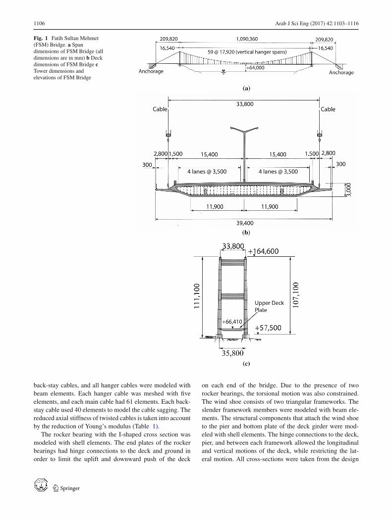
The FSM Bridge is a gravity-anchored suspension bridgewith a length of 1090 m (Fig. 1a). The bridge deck has anaerodynamic cross section similar to the Severn Bridge inEngland (span of 988 m), First Bosporus Bridge in Istan-bul (span of 1074 m), and Humber Bridge in England (spanof 1410 m). The 3 m high and 39.40 m wide bridge deckis a hollow steel box composed of orthotropic stiffenedpanels (Fig. 1b). Diaphragm wall panels are present in thedeck structure at approximately every 4 m. Two steel tow-ers (Fig. 1c) with a height of 107.1 m support the suspensioncables. Each suspension cable is connected to the bridge deckwith 60 vertical hanger cables at intervals of 17.92 m. Thediameter of the suspension cable in the main span is 0.77 m.Themaximum suspension cable force at the top of the towersis 181 MN. The diameter of the back-stay cable is 0.80 mand supports an axial tensile force of 200 MN. The deck,towers, and cables have masses of 16960, 6820, and 10250 t,respectively [13]. The bridge was designed according to theprovisions of the British Standard with some modificationsaccording to the Japanese Industrial Standards.
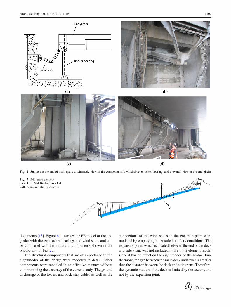
The base of each tower leg is embedded in the reinforcedconcrete foundation to fix the towers at the base. The saddlesare fixed to the top of the towers. Figure 2a shows a schematicof the relevant structural components at both ends of themainspan. A single wind shoe—also called a shear key—connectsthe end segment of the steel deck to the top of the reinforcedconcrete pier as illustrated in Fig. 2b. The wind shoe only
restrains the transverse movement of the bridge. In addition,two rocker bearings connect the deck to the reinforced con-crete pier at each end. A single rocker bearing is shown inFig. 2c. The two rocker bearings at each end resist the verticalmovement of the end girder and provide torsional restraintat each end of the bridge. Figure 2d shows the bottom plateof the end girder, concrete pier, wind shoe, and one of therocker bearings. Additionally, expansion joints are located atboth ends of the main span, separating the deck from the sidespans. Their only purpose is to carry the traffic to and fromthe bridge, and they have no capacity to guide or restrain anymovement of the deck.
3 Finite Element Model of FSM Bridge
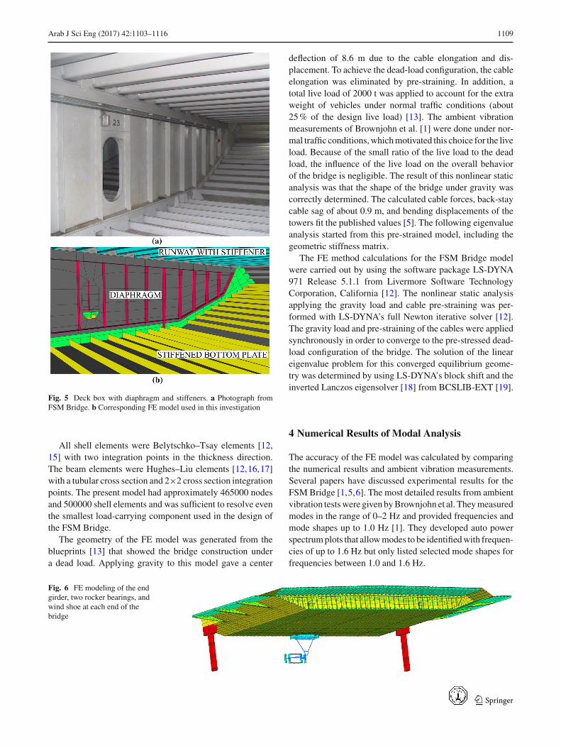
A full three-dimensional FE model [14] of the bridge withcables, a deck body, and towers including all stiffeners wasconsidered for computation with the established finite ele-ment software LS-DYNA [12] (Fig. 3). All steel plates weremodeled with shell finite elements based on the correspond-ing thickness values available in the design documents [13].The curvature of the deck along the longitudinal direction ofthe bridge was modeled; this is important for the coupling ofthe lateral and torsional modes.
The deck and the towers are hollow box structures con-sisting of steel plates with stiffener plates. The four-nodethin shell finite elements offered the most detailed choice formodeling the individual steel plate components of the deckand towers, including all of the stiffener plates. Figure 4ashows the mesh of a tower section with the floors and stiff-ener plates. The tower is reinforced with vertical stiffenerplates placed perpendicular to the main plates. The tower leghas 40 floors along the height and was modeled with about13800 shell elements. The four saddle masses, each of about10 mt, were included as rigid bodies between the top andmain suspension cable. The rigid connection of tower legsto the solid rock is defined by fixed constraints at the towerbase. The bridge deck is made up of 62 segments weldedtogether. The typical span length is 17920 mm. Figure 4bshows a transparent view of the FE model for an individualdeck segment with diaphragms and stiffeners. Table 1 showsthe elastic material properties necessary for the eigenvalueanalysis, while Table 2 covers the range of cross-sectionalproperties for structural members.
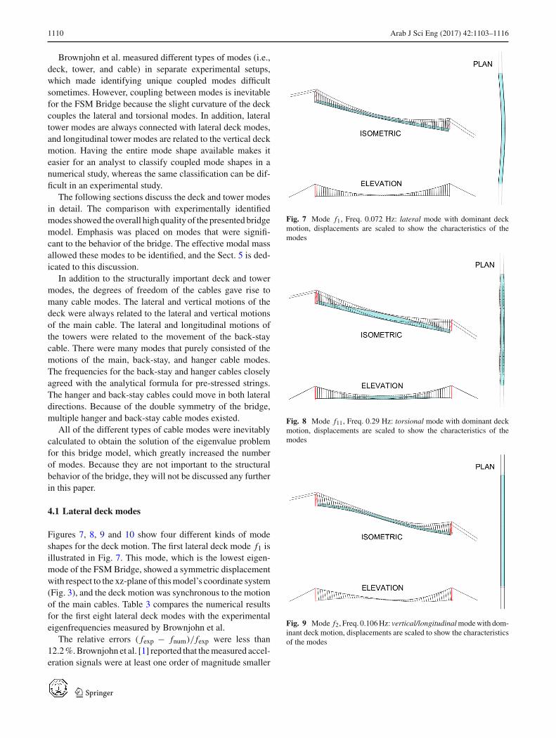
Figure 5a shows a photograph taken inside the deck struc-ture, and Fig. 5b is the corresponding FE model. Each of the62 segments required about 7100 shell elements to model allsignificant components like the stiffeners of the steel con-struction. The mass of the asphalt road cover was taken intoaccount.
The twin hanger cables were modeled as a single cable byusing the resultant cross-sectional area. The main cables, the
123
1106 Arab J Sci Eng (2017) 42:1103–1116
Fig. 1 Fatih Sultan Mehmet(FSM) Bridge. a Spandimensions of FSM Bridge (alldimensions are in mm) b Deckdimensions of FSM Bridge cTower dimensions andelevations of FSM Bridge
back-stay cables, and all hanger cables were modeled withbeam elements. Each hanger cable was meshed with fiveelements, and each main cable had 61 elements. Each back-stay cable used 40 elements to model the cable sagging. Thereduced axial stiffness of twisted cables is taken into accountby the reduction of Young’s modulus (Table 1).
The rocker bearing with the I-shaped cross section wasmodeled with shell elements. The end plates of the rockerbearings had hinge connections to the deck and ground inorder to limit the uplift and downward push of the deck
on each end of the bridge. Due to the presence of tworocker bearings, the torsional motion was also constrained.The wind shoe consists of two triangular frameworks. Theslender framework members were modeled with beam ele-ments. The structural components that attach the wind shoeto the pier and bottom plate of the deck girder were mod-eled with shell elements. The hinge connections to the deck,pier, and between each framework allowed the longitudinaland vertical motions of the deck, while restricting the lat-eral motion. All cross-sections were taken from the design
123
Arab J Sci Eng (2017) 42:1103–1116 1107
Fig. 2 Support at the end of main span: a schematic view of the components, b wind shoe, c rocker bearing, and d overall view of the end girder
Fig. 3 3-D finite elementmodel of FSM Bridge modeledwith beam and shell elements
documents [13]. Figure 6 illustrates the FE model of the endgirder with the two rocker bearings and wind shoe, and canbe compared with the structural components shown in thephotograph of Fig. 2d.
The structural components that are of importance to theeigenmodes of the bridge were modeled in detail. Othercomponents were modeled in an effective manner withoutcompromising the accuracy of the current study. The groundanchorage of the towers and back-stay cables as well as the
connections of the wind shoes to the concrete piers weremodeled by employing kinematic boundary conditions. Theexpansion joint, which is located between the end of the deckand side span, was not included in the finite element modelsince it has no effect on the eigenmodes of the bridge. Fur-thermore, the gap between themain deck and tower is smallerthan the distance between the deck and side spans. Therefore,the dynamic motion of the deck is limited by the towers, andnot by the expansion joint.
123

1108 Arab J Sci Eng (2017) 42:1103–1116
Fig. 4 FE model of tower anddeck parts. The skin istransparent in order to show thestiffener plates inside. a Towersection with stiffeners andfloors. b Single deck segmentwith runway, sideway,diaphragms, and stiffeners
Table 1 Material propertiesDensity (kg/m3) Young’s modulus (MPa) Poisson’s ratio
Deck 8680 210,000 0.3
Tower 8680 210,000 0.3
Main cable 8530 189,300 0.3
Back-stay cable 8530 189,300 0.3
Hanger cable 8530 89,100 0.3
Table 2 Cross-sectionalproperties
Thick. of outer plates Thick. of stiffener plates Areatmin–tmax (mm) tmin–tmax (mm) (mm2)
Deck 10–14 8–16
Tower 60–63 12–20
Main cable 366,160
Back-stay cable 391,301
Hanger cable 5064
123
Arab J Sci Eng (2017) 42:1103–1116 1109
Fig. 5 Deck box with diaphragm and stiffeners. a Photograph fromFSM Bridge. b Corresponding FE model used in this investigation
All shell elements were Belytschko–Tsay elements [12,15] with two integration points in the thickness direction.The beam elements were Hughes–Liu elements [12,16,17]with a tubular cross section and 2×2 cross section integrationpoints. The present model had approximately 465000 nodesand 500000 shell elements and was sufficient to resolve eventhe smallest load-carrying component used in the design ofthe FSM Bridge.
The geometry of the FE model was generated from theblueprints [13] that showed the bridge construction undera dead load. Applying gravity to this model gave a center
deflection of 8.6 m due to the cable elongation and dis-placement. To achieve the dead-load configuration, the cableelongation was eliminated by pre-straining. In addition, atotal live load of 2000 t was applied to account for the extraweight of vehicles under normal traffic conditions (about25% of the design live load) [13]. The ambient vibrationmeasurements of Brownjohn et al. [1] were done under nor-mal traffic conditions,whichmotivated this choice for the liveload. Because of the small ratio of the live load to the deadload, the influence of the live load on the overall behaviorof the bridge is negligible. The result of this nonlinear staticanalysis was that the shape of the bridge under gravity wascorrectly determined. The calculated cable forces, back-staycable sag of about 0.9 m, and bending displacements of thetowers fit the published values [5]. The following eigenvalueanalysis started from this pre-strained model, including thegeometric stiffness matrix.
The FE method calculations for the FSM Bridge modelwere carried out by using the software package LS-DYNA971 Release 5.1.1 from Livermore Software TechnologyCorporation, California [12]. The nonlinear static analysisapplying the gravity load and cable pre-straining was per-formed with LS-DYNA’s full Newton iterative solver [12].The gravity load and pre-straining of the cables were appliedsynchronously in order to converge to the pre-stressed dead-load configuration of the bridge. The solution of the lineareigenvalue problem for this converged equilibrium geome-try was determined by using LS-DYNA’s block shift and theinverted Lanczos eigensolver [18] from BCSLIB-EXT [19].
4 Numerical Results of Modal Analysis
The accuracy of the FE model was calculated by comparingthe numerical results and ambient vibration measurements.Several papers have discussed experimental results for theFSM Bridge [1,5,6]. The most detailed results from ambientvibration testswere given byBrownjohn et al. Theymeasuredmodes in the range of 0–2 Hz and provided frequencies andmode shapes up to 1.0 Hz [1]. They developed auto powerspectrumplots that allowmodes to be identifiedwith frequen-cies of up to 1.6 Hz but only listed selected mode shapes forfrequencies between 1.0 and 1.6 Hz.
Fig. 6 FE modeling of the endgirder, two rocker bearings, andwind shoe at each end of thebridge
123
1110 Arab J Sci Eng (2017) 42:1103–1116
Brownjohn et al. measured different types of modes (i.e.,deck, tower, and cable) in separate experimental setups,which made identifying unique coupled modes difficultsometimes. However, coupling between modes is inevitablefor the FSM Bridge because the slight curvature of the deckcouples the lateral and torsional modes. In addition, lateraltower modes are always connected with lateral deck modes,and longitudinal tower modes are related to the vertical deckmotion. Having the entire mode shape available makes iteasier for an analyst to classify coupled mode shapes in anumerical study, whereas the same classification can be dif-ficult in an experimental study.
The following sections discuss the deck and tower modesin detail. The comparison with experimentally identifiedmodes showed the overall highquality of the presented bridgemodel. Emphasis was placed on modes that were signifi-cant to the behavior of the bridge. The effective modal massallowed these modes to be identified, and the Sect. 5 is ded-icated to this discussion.
In addition to the structurally important deck and towermodes, the degrees of freedom of the cables gave rise tomany cable modes. The lateral and vertical motions of thedeck were always related to the lateral and vertical motionsof the main cable. The lateral and longitudinal motions ofthe towers were related to the movement of the back-staycable. There were many modes that purely consisted of themotions of the main, back-stay, and hanger cable modes.The frequencies for the back-stay and hanger cables closelyagreed with the analytical formula for pre-stressed strings.The hanger and back-stay cables could move in both lateraldirections. Because of the double symmetry of the bridge,multiple hanger and back-stay cable modes existed.
All of the different types of cable modes were inevitablycalculated to obtain the solution of the eigenvalue problemfor this bridge model, which greatly increased the numberof modes. Because they are not important to the structuralbehavior of the bridge, they will not be discussed any furtherin this paper.
4.1 Lateral deck modes
Figures 7, 8, 9 and 10 show four different kinds of modeshapes for the deck motion. The first lateral deck mode f1 isillustrated in Fig. 7. This mode, which is the lowest eigen-mode of the FSM Bridge, showed a symmetric displacementwith respect to the xz-plane of thismodel’s coordinate system(Fig. 3), and the deck motion was synchronous to the motionof the main cables. Table 3 compares the numerical resultsfor the first eight lateral deck modes with the experimentaleigenfrequencies measured by Brownjohn et al.
The relative errors ( fexp − fnum)/ fexp were less than12.2%.Brownjohn et al. [1] reported that themeasured accel-eration signals were at least one order of magnitude smaller
Fig. 7 Mode f1, Freq. 0.072 Hz: lateral mode with dominant deckmotion, displacements are scaled to show the characteristics of themodes
Fig. 8 Mode f11, Freq. 0.29 Hz: torsional mode with dominant deckmotion, displacements are scaled to show the characteristics of themodes
Fig. 9 Mode f2, Freq. 0.106Hz: vertical/longitudinalmodewith dom-inant deck motion, displacements are scaled to show the characteristicsof the modes
123
Arab J Sci Eng (2017) 42:1103–1116 1111
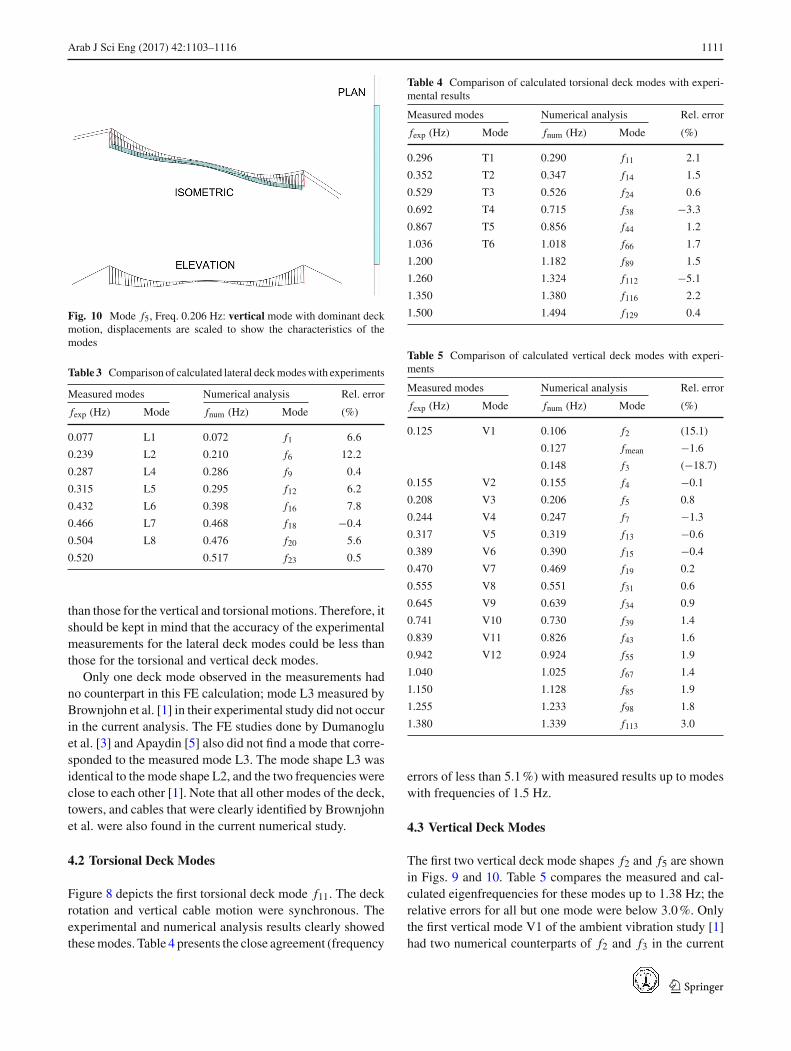
Fig. 10 Mode f5, Freq. 0.206 Hz: vertical mode with dominant deckmotion, displacements are scaled to show the characteristics of themodes
Table 3 Comparison of calculated lateral deckmodeswith experiments
Measured modes Numerical analysis Rel. error
fexp (Hz) Mode fnum (Hz) Mode (%)
0.077 L1 0.072 f1 6.6
0.239 L2 0.210 f6 12.2
0.287 L4 0.286 f9 0.4
0.315 L5 0.295 f12 6.2
0.432 L6 0.398 f16 7.8
0.466 L7 0.468 f18 −0.4
0.504 L8 0.476 f20 5.6
0.520 0.517 f23 0.5
than those for the vertical and torsionalmotions. Therefore, itshould be kept in mind that the accuracy of the experimentalmeasurements for the lateral deck modes could be less thanthose for the torsional and vertical deck modes.
Only one deck mode observed in the measurements hadno counterpart in this FE calculation; mode L3 measured byBrownjohn et al. [1] in their experimental study did not occurin the current analysis. The FE studies done by Dumanogluet al. [3] and Apaydin [5] also did not find a mode that corre-sponded to the measured mode L3. The mode shape L3 wasidentical to the mode shape L2, and the two frequencies wereclose to each other [1]. Note that all other modes of the deck,towers, and cables that were clearly identified by Brownjohnet al. were also found in the current numerical study.
4.2 Torsional Deck Modes
Figure 8 depicts the first torsional deck mode f11. The deckrotation and vertical cable motion were synchronous. Theexperimental and numerical analysis results clearly showedthesemodes. Table 4 presents the close agreement (frequency
Table 4 Comparison of calculated torsional deck modes with experi-mental results
Measured modes Numerical analysis Rel. error
fexp (Hz) Mode fnum (Hz) Mode (%)
0.296 T1 0.290 f11 2.1
0.352 T2 0.347 f14 1.5
0.529 T3 0.526 f24 0.6
0.692 T4 0.715 f38 −3.3
0.867 T5 0.856 f44 1.2
1.036 T6 1.018 f66 1.7
1.200 1.182 f89 1.5
1.260 1.324 f112 −5.1
1.350 1.380 f116 2.2
1.500 1.494 f129 0.4
Table 5 Comparison of calculated vertical deck modes with experi-ments
Measured modes Numerical analysis Rel. error
fexp (Hz) Mode fnum (Hz) Mode (%)
0.125 V1 0.106 f2 (15.1)
0.127 fmean −1.6
0.148 f3 (−18.7)
0.155 V2 0.155 f4 −0.1
0.208 V3 0.206 f5 0.8
0.244 V4 0.247 f7 −1.3
0.317 V5 0.319 f13 −0.6
0.389 V6 0.390 f15 −0.4
0.470 V7 0.469 f19 0.2
0.555 V8 0.551 f31 0.6
0.645 V9 0.639 f34 0.9
0.741 V10 0.730 f39 1.4
0.839 V11 0.826 f43 1.6
0.942 V12 0.924 f55 1.9
1.040 1.025 f67 1.4
1.150 1.128 f85 1.9
1.255 1.233 f98 1.8
1.380 1.339 f113 3.0
errors of less than 5.1%) with measured results up to modeswith frequencies of 1.5 Hz.
4.3 Vertical Deck Modes
The first two vertical deck mode shapes f2 and f5 are shownin Figs. 9 and 10. Table 5 compares the measured and cal-culated eigenfrequencies for these modes up to 1.38 Hz; therelative errors for all but one mode were below 3.0%. Onlythe first vertical mode V1 of the ambient vibration study [1]had two numerical counterparts of f2 and f3 in the current
123
1112 Arab J Sci Eng (2017) 42:1103–1116
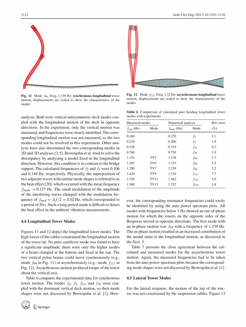
Fig. 11 Mode f99, Freq. 1.239 Hz: synchronous longitudinal towermotion, displacements are scaled to show the characteristics of themodes
analysis. Both were vertical antisymmetric deck modes cou-pled with the longitudinal motion of the deck in oppositedirections. In the experiment, only the vertical motion wasmeasured, and frequencieswere clearly identified. The corre-sponding longitudinal motion was not measured, so the twomodes could not be resolved in this experiment. Other ana-lysts have also determined the two corresponding modes in2D and 3D analyses [3,5]. Brownjohn et al. tried to solve thediscrepancy by analyzing a model fixed in the longitudinaldirection. However, this condition is in contrast to the bridgesupport. The calculated frequencies of f2 and f3 were 0.106and 0.148 Hz, respectively. Physically, the superposition oftwo adjacent waves with similar mode shapes is referred to asthe beat effect [20], which occurred with the mean frequencyfmean = 0.127 Hz. The small modulation of the amplitudeof the interfering waves changed with the modulation fre-quency of fmod = � f/2 = 0.02Hz, which corresponded toa period of 50 s. Such a long period made it difficult to detectthe beat effect in the ambient vibration measurements.
4.4 Longitudinal Tower Modes
Figures 11 and 12 depict the longitudinal tower modes. Thehigh forces of the cables constrained the longitudinal motionof the tower tip. No pure cantilever mode was found to havea significant amplitude; there were only the higher modesof a beam clamped at the bottom and fixed at the top. Thetwo vertical pylon beams could move synchronously (e.g.,mode f99 in Fig. 11) or asynchronously (e.g., mode f112 inFig. 12). Asynchronous motion produced torque of the towerabout the vertical axis.
Table 6 compares the experimental data for synchronoustower motion. The modes f4, f5, f13, and f39 were cou-pled with the dominant vertical deck motion, so their modeshapes were not discussed by Brownjohn et al. [1]. How-
Fig. 12 Mode f112, Freq. 1.32 Hz: asynchronous longitudinal towermotion, displacements are scaled to show the characteristics of themodes
Table 6 Comparison of calculated pure bending longitudinal towermodes with experiments
Measured modes Numerical analysis Rel. error
fexp (Hz) Mode fnum (Hz) Mode (%)
0.160 0.155 f4 3.1
0.210 0.206 f5 1.9
0.320 0.319 f13 0.3
0.760 0.730 f39 3.9
1.154 TV5 1.128 f85 2.3
1.265 TV6 1.233 f98 2.5
1.280 TV7 1.239 f99 3.2
1.420 TV9 1.310 f111 7.7
1.538 TV11 1.462 f127 4.9
1.580 TV13 1.552 f139 1.8
ever, the corresponding resonance frequencies could easilybe identified by using the auto power spectrum plots. Allmodes with frequencies below 1 Hz showed an out-of-phasemotion for which the towers on the opposite sides of theBosporus moved in opposite directions. The first mode withan in-phase motion was f99 with a frequency of 1.239 Hz.The in-phase motion resulted in an increased contribution ofthe modal mass to the longitudinal motion, as discussed inthe Sect. 5.
Table 7 presents the close agreement between the cal-culated and measured modes for the asynchronous towermotion. Again, the measured frequencies had to be takenfrom the auto power spectrum plots because the correspond-ing mode shapes were not discussed by Brownjohn et al. [1].
4.5 Lateral Tower Modes
For the lateral response, the motion of the top of the tow-ers was not constrained by the suspension cables. Figure 13
123

Arab J Sci Eng (2017) 42:1103–1116 1113
Table 7 Comparison of calculated longitudinal tower modes withexperiments for modes with bending and torque
Measured modes Numerical analysis Rel. error
fexp (Hz) Mode fnum (Hz) Mode (%)
0.30 0.290 f11 2.7
1.03 1.018 f71 1.1
1.35 1.324 f112 1.9
1.41 1.380 f116 2.1
1.52 1.494 f129 1.7
1.58 1.543 f138 2.3
Fig. 13 Mode f16, Freq. 0.398 Hz: lateral tower motion—basic can-tilever mode, displacements are scaled to show the characteristics of themodes
shows the lateralmotion of the towerwith the basic cantilevermode f16, and Fig. 14 shows that with the higher mode f157.Table 8 lists the frequencies of the lateral tower modes. Inthe lateral tower modes with low frequencies, the tower tipmoved in the lateral direction (Fig. 13) and excited the lateraldeck motion.
5 Modal Mass Analysis
Different modes are important depending on the objective.Cable modes are important for excitation by an aerodynamicdrag load. The lateral, vertical, and torsional modes of thedeck and tower are important to analyzing the displacement
Fig. 14 Mode f157, Freq. 1.657 Hz: lateral tower motion—higherorder mode, displacements are scaled to show the characteristics ofthe modes
Table 8 Comparison of calculated lateral tower modes with experi-mental results
Measured modes Numerical analysis Rel. error
fexp (Hz) Mode fnum (Hz) Mode (%)
0.287 TL1 0.286 f9 0.3
0.295 TL2 0.295 f12 0.0
0.385 0.398 f16 −3.4
0.432 TL3 0.468 f18 −8.3
0.464 TL4 0.476 f20 −2.6
0.503 TL5 0.509 f22 −1.2
0.520 TL6 0.517 f23 0.6
0.630 TL7 0.601 f32 3.4
0.673 TL8 0.678 f35 −0.7
0.692 TL9 0.686 f36 0.9
0.753 TL10 0.767 f40 −1.9
0.802 TL11 0.825 f42 −2.9
0.866 TL12 0.881 f45 −1.7
0.937 TL13 0.955 f56 −1.9
1.200 TL17 1.154 f87 3.8
1.370 TL20 1.369 f115 0.1
1.712 TL26 1.691 f163 1.2
123

1114 Arab J Sci Eng (2017) 42:1103–1116
Table 9 Transitional modal masses of eigenmodes with contributionsgreater than 5% of total mass
Mode Freq. (Hz) Effective modal mass (%)
x-trans. y-trans. z-trans.
f1 0.072 61.07 − −f2 0.106 − 27.20 −f3 0.148 − 29.23 −f4 0.156 − − 20.28
f5 0.206 − − 41.55
f16 0.398 9.73 − −f22 0.509 10.04 − −f29 0.550 − − 6.75
f99 1.239 − 29.80 −∑
modal masses 80.84 86.23 68.58
and stresses of the bridge structure. The effectivemass allowsthe significance of a mode to be quantified. Table 9 lists theeffective masses (as percentages of the total mass of the FSMBridge) of the important modes for synchronous excitationsof both towers. Symmetric lateral, vertical, and longitudinalmodes contributed to the effective mass.
Modes with transitional modal masses larger than 5% ofthe total mass are included in Table 9. The first five modes,which are deckmodes, containedmore than 50%of the effec-tive mass in each direction. Modes up to 0.509 Hz needed becalculated in order to reach 80% of the effective modal massin the lateral direction (x-direction) as listed on the line ’
∑
modal masses’. For the longitudinal direction (y-direction),modes with frequencies up to 1.239 Hz needed be analyzedto incorporate 80% of the effective mass. Vertical modes upto 0.55 Hz contributed more than 5% in the z-direction. Inorder to include 80% of the total effective mass in the z-direction, three modes with single contributions below 5%had to be considered. One of these modes had a frequencyhigher than 10 Hz owing to the stiff response of the towersin the vertical direction.
The coupled lateral deck tower modes f16 and f22contributed to the lateral modal mass because theywere sym-metric. Only one cablemodewith a frequency of 0.55Hz hada significant modal mass, which had its origin in the synchro-nous symmetric vertical swinging of all back-stay cables, butit was not important to the structural properties of the FSMBridge. Mode f99 with a frequency of 1.239 Hz was the onlytower mode with significant modal mass in the longitudinaldirection. As pointed out in the Sect. 4.4, this was due tothe synchronous longitudinal motion in this mode; all lowerlongitudinal tower modes were asynchronous, which led tothe cancellation of the modal masses.
Several previous studies focused on describing the first 40eigenmodes up to 0.8Hz.Based on themodalmasses, the first
40 modes were not sufficient to capture all of the importantmodal mass contributions. That is, the accumulated modalmass was well below 80% of the physical total mass in twodirections. In fact, the eigenmodes needed to be computedwith frequencies up to 11Hz in order to reach an accumulatedmodal mass of around 90% in all three directions.
6 Comparison of Beam and Shell FE Models forTorsional Modes of the FSM Bridge
In order to illustrate the difficulty inmodeling the orthotropicdeck structure of the FSM Bridge using beam elements,Table 8 provides the comparison of modal frequenciesbetween the ambient vibration test results [1] and the calcu-lations of the FE models for the torsional modes T1 throughT5. The beam FEmodel included the deck, tower, and rockerbearings of the FSM Bridge [5,6]. The shell FE model ofthis study provided closer results to the ambient vibrationtest measurements for all the modes given in Table 10. Therelative error of the beam model was at least one orderof magnitude higher than the shell model. The orthotropicdeck structure with internal diaphragms and stiffeners wereonly approximately represented by a single torsional constantin the cross-sectional input properties of the beam model,whereas the shellmodel included such structural componentsexplicitly in the analysis of the bridge.
7 Conclusions and Recommendations for FutureWork
Modeling all of the thin steel plates of a structure with shellelements and the cables with beam elements is a straightfor-ward procedure to generate a model from structural designdocuments. The analysis showed that this approach provideda high-fidelity model of the suspension bridge. Modern FEtools allow the efficient generation and solution of this largemodel. The LS-DYNA commercial finite element code wasused to investigate the free vibration modes of the FSMSuspension Bridge. No effective cross-sections need to beestimated or fitted to the experimental results. All majorstiffener plates and load-carrying structural components areincluded. The parameter-free FE model removes the needfor calibration when compared with the beam models ofsuspension bridges that require the iterative calibration ofthe cross-sectional area, moments of inertia, and torsionalconstants. In contrast to beam models, the proposed modelincludes the deck cross-sectional deformations caused by therocker bearings andwind shoes.All of the natural frequenciesof the bridge for lateral, vertical, longitudinal, and torsionalbehaviors can be calculated with this 3D model with goodaccuracy into the high frequency range. The benefit of the
123

Arab J Sci Eng (2017) 42:1103–1116 1115
Table 10 Comparison of torsional mode frequencies for the shell and beam FE models
Torsionalmode number
Measured ambientvibration freq. (Hz)
Shell model com-puted freq. (Hz)
Rel. error of shellmodel (%)
Beam modelcomputed freq.(Hz)
Rel. error of beammodel (%)
T1 0.296 0.290 2.1 0.387 −31
T2 0.352 0.347 1.5 0.417 −19
T3 0.529 0.526 0.6 0.633 −20
T4 0.692 0.715 −3.3 0.799 −16
T5 0.867 0.856 1.2 1.026 −18
model is that all coupling effects between different modesand the different components of the deck, towers, and cablesare automatically included, while the limited number of sen-sors placed on the structuremakes identifying coupledmodesin an experiment challenging.
The comparison of the calculated coupled modes andexperimental results led to a better understanding of the phys-ical behavior of the bridge, as shown for the deck and towermodes. There is only a single measured mode that corre-sponds to the calculated frequencies of the modes f2 and f3.The discrepancy was attributed to the superposition of thesetwo modes via the beat effect, as discussed in the Sect. 4.3.The ambient vibration measurements were carried out underweak wind conditions, which resulted in weak amplitudesfor the lateral modes as discussed in the Sect. 4.1. There-fore, the accuracy of the measured frequencies was less forthe lateral modes of the deck, while the calculated verticaland torsional deck mode frequencies were reproduced withrelative errors below roughly 5%. All tower mode frequen-cies fit the measured values with relative errors of less than9%. Contrast between the beam and shell FE models of thebridge was demonstrated for the results of the torsional modefrequencies.
Using the effectivemodalmass as a criterion for importantmodes made it clear that modes up to a frequency of around1.2Hzmust be identifiedwhen analyzing the dynamic behav-ior with modal superposition methods. A single mode with afrequency of 1.24Hz had an effective modal mass contribu-tion of about 30% of the total mass and was a longitudinaltower mode that occurred at a high frequency due to the highaxial forces of the suspension and back-stay cables. Only amodel that includes the stiffened structure of the towers andthe realistic cable forces at the same time can describe suchan important mode.
This model can be used with not only the response spec-trum approach and modal superposition method but also innonlinear time history analyseswith explicit time integration.The detailedmodel resolves local stress concentrations in thedeck and tower components to identify fatigue damage andlocalized plastic strain under extreme loads. The next phaseof the study will involve using the developed model as an
approved basis for further nonlinear seismic analysis of theFSM Bridge, such as investigating severe events where thedeck and towers are impacted.
Acknowledgements The first author is grateful to the funding pro-vided by TUBITAK (Turkish Scientific and Technological ResearchCouncil) through research Grant 107M002 and by the Bogazici Uni-versity Research Fund through Contract 07HT102.
Open Access This article is distributed under the terms of the CreativeCommons Attribution 4.0 International License (http://creativecommons.org/licenses/by/4.0/), which permits unrestricted use, distribution,and reproduction in any medium, provided you give appropriate creditto the original author(s) and the source, provide a link to the CreativeCommons license, and indicate if changes were made.
References
1. Brownjohn, J.M.W.; Dumanoglu, A.A.; Severn, R.T.: Ambientvibration survey of the Fatih Sultan Mehmet (Second Bosporus)suspension bridge. Earthq. Eng. Struct. D. 21, 907–24 (1992)
2. Brownjohn, J.M.W.; Severn, R.T.; Dumanoglu, A.A.: Full-scaledynamic testing of the 2nd Bosporus suspension bridge. In:Proceedings of the Tenth World Conference on Earthquake Engi-neering, Madrid, Spain, pp. 2695–700 (1992)
3. Dumanoglu, A.A.; Brownjohn, J.M.W.; Severn, R.T.: Seismicanalysis of the Fatih Sultan Mehmet (2nd Bosporus) suspensionbridge. Earthq. Eng. Struct. D. 21, 881–906 (1992)
4. Abdel-Ghaffar, A.M.; Stringfellow, R.G.: Response of suspen-sion bridges to travelling earthquake excitations: part II. Lateralresponse. Soil Dyn. Earthq. Eng. 3, 73–81 (1984)
5. Apaydin, N.M.: Seismic analysis of Fatih Sultan Mehmet Suspen-sion Bridge. Ph.D. thesis, Department of Earthquake Engneering,Bogazici University, Istanbul, Turkey (2002)
6. Apaydin, N.M.: Earthquake performance assessment and retrofitinvestigations of two suspension bridges in Istanbul. Soil Dyn.Earthq. Eng. 30, 702–10 (2010)
7. Daniell, W.E.; Macdonald, J.H.G.: Improved finite element mod-elling of a cable-stayed bridge through systematic manual tuning.Eng. Struct. 29, 358–71 (2007)
8. Zhang, J.; Prader, J.; Moon, F.; Aktan, E.; Wu, Z.S.: Challengesand strategies in structural identification of a long span suspensionbridge. In: 6th International Workshop on Advanced Smart Mate-rials and Smart Structures Technology (ANCRiSST), Dalian, pp1–12 (2011)
9. Rahbari, A.R.; Brownjohn, J.M.W.: Finite element modelling ofHumber Bridge. In: 6th International Conference on Bridge Main-
123
1116 Arab J Sci Eng (2017) 42:1103–1116
tenance, Safety and Management (IABMAS), Stresa, pp. 3709–16(2012)
10. Karmakar, D.; Ray-Chaudhuri, S.; Shinozuka, M.: Finite elementmodel development, validation and probabilistic seismic perfor-mance evaluation of Vincent Thomas suspension bridge. Struct.Infrastruct. E. 11(2), 223–237 (2015)
11. Duan, Y.F.; Xu, Y.L.; Fei, Q.G.; Wong, K.Y.; Chan, K.W.Y.; Ni,Y.Q.; Ng, C.L.: Advanced finite elementmodel of TsingMaBridgefor structural health monitoring. Int. J. Struct. Stab. Dyn. 11, 313–344 (2011)
12. Hallquist, J.O.: LS-DYNATheoryManual. LSTC (LivermoreSoft-ware Technology Corporation), Livermore, California (2006)
13. IHI, MHI, NKK Corp.: Record Book for the Fatih Sultan MehmetSuspension Bridge. Tokyo (1989)
14. Ingenlath, P.: Seismic Finite Element Analysis of the SecondBosporus Bridge. Bachelor Engineering thesis, Department ofMechanical Engineering, Aachen University of Applied Sciences,Aachen (2010)
15. Belytschko, T.B.; Tsay, C.S.: Explicit algorithms for the nonlineardynamics of shells. Comput. Method. Appl. Mech. Eng. 42, 225–251 (1984)
16. Hughes, T.J.R.; Liu, W.K.: Nonlinear finite element analysis ofshells: part I. Three-dimensional shells. Comput. Method. Appl.Mech. Eng. 26, 331–362 (1981)
17. Hughes, T.J.R.; Liu, W.K.: Nonlinear finite element analysis ofshells: part II. Two-dimensional shells. Comput. Method. Appl.Mech. Eng. 27, 167–181 (1981)
18. Grimes, R.; Lewis, J.; Simon, H.: A shifted block Lanczos algo-rithm for solving sparse symmetric generalized eigenproblems.SIAM J. Matrix Anal. Appl. 15, 228–272 (1994)
19. The Boeing Company: Boeing Extreme Mathematical Library(BCSLIB-EXT) User’s Guide. Seattle, Washington (2000)
20. Feynman, R.P.; Sands, M.; Leighton, R.: The Feynman Lectureson Physics. Addison Wesley, Boston (2006)
123