FEA Information Engineering Journal Information Engineering Journal February 2014.pdf · FEA Information Engineering Journal (FEAIEJ™) is a monthly published online journal to cover

ISSN 2167-1273 Volume 3, Issue 2, February 2014

FEA Information Engineering Journal

Civil & Offshore Engineering


Aim and Scope FEA Information Engineering Journal (FEAIEJ™) is a monthly published online journal to cover the latest Finite Element Analysis Technologies. The journal aims to cover previous noteworthy published papers and original papers. All published papers are peer reviewed in the respective FEA engineering fields. Consideration is given to all aspects of technically excellent written information without limitation on length. All submissions must follow guidelines for publishing a paper, or periodical. If a paper has been previously published, FEAIEJ requires written permission to reprint, with the proper acknowledgement give to the publisher of the published work. Reproduction in whole, or part, without the express written permissio of FEA Information Engineering Journal, or the owner of of the copyright work, is strictly prohibited. FEAIJ welcomes unsolicited topics, ideas, and articles. Monthly publication is limited to no more then five papers, either reprint, or original. Papers will be archived on www.feaiej.com For information on publishing a paper original or reprint contact [email protected] Subject line: Journal Publication

Fig. 7: Different fringe plots. A Quadratic Pipe Element in LS-DYNA® Tobias Olsson, Daniel Hilding DYNAmore Nordic AB

2 Fea Information Engineering Journal February 2014

http://www.feaiej.com/

mailto:[email protected]


TABLE OF CONTENTS

Publications are © to LS-DYNA 2013 9th European Users‘ Conference

A Quadratic Pipe Element in LS-DYNA® Tobias Olsson, Daniel Hilding DYNAmore Nordic AB Seismic Response of Baffled Liquid Containment Tanks Zuhal Ozdemir1, Yasin Fahjan2 and Mhamed Souli3 1 Department of Civil and Structural Engineering, University of Sheffield, UK 2 Department of Earthquake and Structural Engineering, Gebze Institute of Technology, Turkey 3 Laboratoire de Mécanique de Lille, Université des Sciences et des Technologies de Lille, France

All contents are copyright © to the publishing company, author or respective company. All rights reserved.

3 Fea Information Engineering Journal February 2014

© 2013 Copyright by Arup

A Quadratic Pipe Element in LS-DYNA®

Tobias Olsson, Daniel Hilding

DYNAmore Nordic AB

1 Background Analysis of long piping structures can be challenging due to the enormous number of shell/solid elements that would be required to model a piping structure accurate. In that context a new beam element has been developed that can, if used correctly, reduce the number of elements used in a pipe simulation. Since it is constructed of 3 nodes it is perfect for describing pipe bends, so called elbows. This document is meant as an introduction and modelling techniques for the elbow element. It is implemented in LS-DYNA® R7.0.0 but improvements are implemented in the coming update of LS-DYNA R7 [1].

2 Theory The main theory is based on the work done by Almeida [2] The beam is formulated under the plane stress assumption and with thin shell theory. That means that the quotient between the thickness of the tube (t) and the outer radius (a) should be small and the quotient between the radius and the pipe curvature (R) should also be small. 𝑡𝑎≪ 1, 𝑎

𝑅≪ 1 (1)

The basic assumption is that plane sections originally normal to the center line remain plane but not necessarily normal. The following displacement formula holds for a point in the element after deformation

𝑢𝑖(𝑟, 𝑠, 𝑡) = ∑ ℎ𝑘(𝑟)𝑢𝑖𝑘 + ∑ 𝑎𝑘ℎ𝑘(𝑟)�𝑡𝑉𝑡𝑖𝑘 + 𝑠𝑉𝑠𝑖𝑘�, 𝑖 = 1,2,33𝑘=1

3𝑘=1 (2)

Where 𝑟, 𝑠, 𝑡 are iso-parametric coordinates, 𝑢𝑖 is the displacement at any point in the pipe element, ℎ𝑘 is the interpolation function and 𝑢𝑖𝑘 is the displacement of node 𝑘 in the current element. The 𝑉𝑡𝑖𝑘 and 𝑉𝑠𝑖𝑘 are the components of the rotated orientation vectors along the t and s directions, and 𝑎𝑘 is the outer pipe radius. We calculate 𝑽𝑠𝑘 and 𝑽𝑡𝑘 as the cross product between the nodal rotation increment and the ”old” orientation vector.

𝑽𝑠𝑘 = ∆𝜽𝑘 × 𝑽𝑠0𝑘 (3)

𝑽𝑡𝑘 = ∆𝜽𝑘 × 𝑽𝑡0𝑘 The current beam displacements assume that the cross section of the pipe does not deform. To include the ovalization to the formulation we introduce a new displacement field as follows

𝑤(𝑟,𝜙) = ∑ ∑ ℎ𝑘(𝑟)(𝑐𝑚𝑘 sin 2𝑚𝜙 + 𝑑𝑚𝑘 cos 2𝑚𝜙)3𝑘=1

3𝑚=1 (4)

Where 𝑐𝑚𝑘 and 𝑑𝑚𝑘 are generalized ovalization displacements. The total displacement is calculated as the sum of 𝑢 and 𝑤 which give the beam a total of 12 degrees of freedom per node.

9th European LS-DYNA Conference 2013 _________________________________________________________________________________


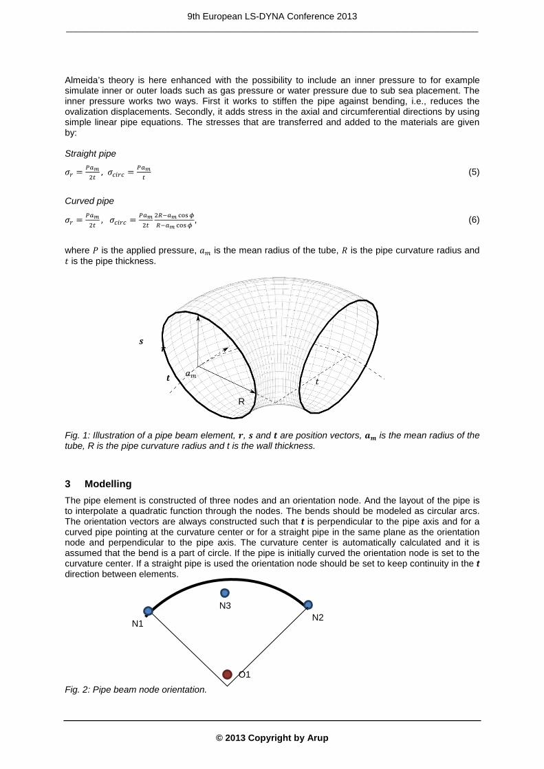
Almeida’s theory is here enhanced with the possibility to include an inner pressure to for example simulate inner or outer loads such as gas pressure or water pressure due to sub sea placement. The inner pressure works two ways. First it works to stiffen the pipe against bending, i.e., reduces the ovalization displacements. Secondly, it adds stress in the axial and circumferential directions by using simple linear pipe equations. The stresses that are transferred and added to the materials are given by: Straight pipe

𝜎𝑟 = 𝑃𝑎𝑚2𝑡

, 𝜎𝑐𝑖𝑟𝑐 = 𝑃𝑎𝑚𝑡

(5)

Curved pipe

𝜎𝑟 = 𝑃𝑎𝑚2𝑡

, 𝜎𝑐𝑖𝑟𝑐 = 𝑃𝑎𝑚2𝑡

2𝑅−𝑎𝑚 cos𝜙𝑅−𝑎𝑚 cos𝜙

, (6)

where 𝑃 is the applied pressure, 𝑎𝑚 is the mean radius of the tube, 𝑅 is the pipe curvature radius and 𝑡 is the pipe thickness.

Fig. 1: Illustration of a pipe beam element, 𝒓, 𝒔 and 𝒕 are position vectors, 𝒂𝒎 is the mean radius of the tube, R is the pipe curvature radius and t is the wall thickness.

3 Modelling The pipe element is constructed of three nodes and an orientation node. And the layout of the pipe is to interpolate a quadratic function through the nodes. The bends should be modeled as circular arcs. The orientation vectors are always constructed such that t is perpendicular to the pipe axis and for a curved pipe pointing at the curvature center or for a straight pipe in the same plane as the orientation node and perpendicular to the pipe axis. The curvature center is automatically calculated and it is assumed that the bend is a part of circle. If the pipe is initially curved the orientation node is set to the curvature center. If a straight pipe is used the orientation node should be set to keep continuity in the t direction between elements. Fig. 2: Pipe beam node orientation.

𝒓

R

𝒔

𝒕 𝑎𝑚 𝑡

N1 N2

N3

O1



3.1 Input example (Element)

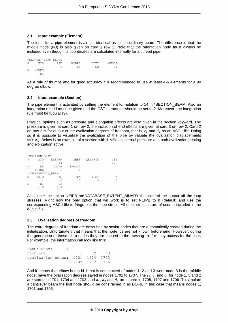
The input for a pipe element is almost identical as for an ordinary beam. The difference is that the middle node (N3) is also given on card 1 row 2. Note that the orientation node must always be included even though its coordinates are calculated internally for a curved pipe: *ELEMENT_BEAM_ELBOW $ EID PID NODE1 NODE2 ONODE 1 1 N1 N2 O1 $ NODE3 N3 As a rule of thumbs and for good accuracy it is recommended to use at least 4-6 elements for a 90 degree elbow.

3.2 Input example (Section)

The pipe element is activated by setting the element formulation to 14 in *SECTION_BEAM. Also an integration rule id must be given and the CST parameter should be set to 2. Moreover, the integration rule must be tubular (9). Physical options such as pressure and elongation effects are also given in the section keyword. The pressure is given at card 1 on row 2, the inclusion of end effects are given at card 3 on row 2. Card 2 on row 2 is for output of the ovalization degrees of freedom, that is, 𝑐𝑘 and 𝑑𝑘 as an ASCII-file. Doing so it is possible to visualize the ovalization of the pipe by valuate the ovalization displacements 𝑤(𝑟,𝜙). Below is an example of a section with 1 MPa as internal pressure and both ovalization printing and elongation active. *SECTION_BEAM $ SID ELFORM SHRF QR/IRID CST 1 14 1.0 -1 2.0 $ PR IOVPR IPRSTR 1.0E6 1 1 *INTEGRATION_BEAM $ IRID NIP RA ICST K 1 0 0 9 0 $ D1 D2 1.0 0.7 Also, note the option NEIPB on*DATABASE_EXTENT_BINARY that control the output off the loop stresses. Right now the only option that will work is to set NEIPB to 0 (default) and use the corresponding ASCII-file to fringe plot the loop-stress. All other stresses are of course included in the d3plot file.

3.3 Ovalization degrees of freedom

The extra degrees of freedom are described by scalar nodes that are automatically created during the initialization. Unfortunately that means that the node ids are not known beforehand. However, during the generation of these extra nodes they are echoed to the messag file for easy access for the user. For example, the information can look like this: ELBOW BEAM: 1 n1-n3-n2: 1 2 3 ovalization nodes: 1701 1704 1703 1705 1707 1706 And it means that elbow beam id 1 that is constructed of nodes 1, 2 and 3 were node 3 is the middle node, have the ovalization degrees saved in nodes 1701 to 1707. The 𝑐1, 𝑐2 and 𝑐3 for node 1, 3 and 2 are stored in 1701, 1704 and 1703, and 𝑑1, 𝑑2 and 𝑑3 are stored in 1705, 1707 and 1706. To simulate a cantilever beam the first node should be constrained in all DOFs. In this case that means nodes 1, 1701 and 1705.



If the IOVPR flag is set, then the ovalization displacements for each element are written to an ASCII file ‘elbwov’. They can be used for further analysis of the pipe. For example the total ovalization of the pipe can be calculated by using the displacement formula above. The format for the ASCII file is as follows (spaces have been removed to fit this page): OVALIZATION D.O.F. WITH PRESSURE: 1.210E+06 (TIME = 1.000000) BEAM ID: 1 c1 c2 c3 d1 d2 d3 NODE 1: 0.35E-4 -0.49E-5 0.16E-6 -0.40E-3 -0.19E-4 -0.15E-5 NODE 2: 0.46E-4 0.28E-5 -0.77E-7 0.36E-3 0.23E-4 0.52E-4 NODE 3: 0.11E-3 -0.74E-5 0.14E-6 0.16E-2 -0.84E-4 0.10E-3 Note that the ovalization nodes only have translation degrees of freedom. That means that velocity boundary conditions cannot be set.

3.4 Contacts

Due to the extra node in this formulation the beam contacts will not work for curved beams. If a beam contact is used the curved beam will be treated as a linear beam between node 1 and 2. Node to node contacts and node to surface contacts should work as usual but the curved beam between the nodes will not be added to the contact.

4 Examples In LS-PrePost® 4.1 or newer a new rendering engine is implemented that can visualize the pipes as curved beams, see Fig. 3. All that is needed is that the k-file is used together with the d3plot file and that the CST flag is set to 2.

4.1 Two elements Cantilever beam

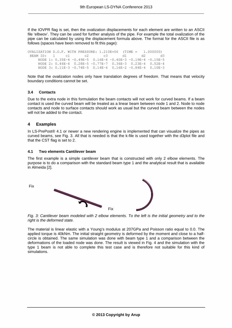
The first example is a simple cantilever beam that is constructed with only 2 elbow elements. The purpose is to do a comparison with the standard beam type 1 and the analytical result that is available in Almeida [2].

Fig. 3: Cantilever beam modeled with 2 elbow elements. To the left is the initial geometry and to the right is the deformed state. The material is linear elastic with a Young’s modulus at 207GPa and Poisson ratio equal to 0.0. The applied torque is 40kNm. The initial straight geometry is deformed by the moment and close to a half-circle is obtained. The same simulation was done with beam type 1 and a comparison between the deformations of the loaded node was done. The result is viewed in Fig. 4 and the simulation with the type 1 beam is not able to complete this test case and is therefore not suitable for this kind of simulations.

Fix

Fix



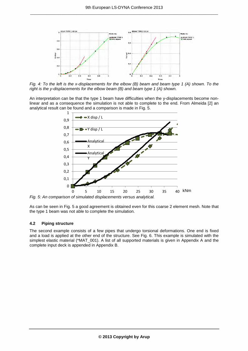
Fig. 4: To the left is the x-displacements for the elbow (B) beam and beam type 1 (A) shown. To the right is the y-displacements for the elbow beam (B) and beam type 1 (A) shown. An interpretation can be that the type 1 beam have difficulties when the y-displacements become non-linear and as a consequence the simulation is not able to complete to the end. From Almeida [2] an analytical result can be found and a comparison is made in Fig. 5.

Fig. 5: An comparison of simulated displacements versus analytical. As can be seen in Fig. 5 a good agreement is obtained even for this coarse 2 element mesh. Note that the type 1 beam was not able to complete the simulation.

4.2 Piping structure

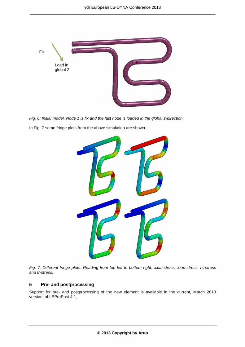
The second example consists of a few pipes that undergo torsional deformations. One end is fixed and a load is applied at the other end of the structure. See Fig. 6. This example is simulated with the simplest elastic material (*MAT_001). A list of all supported materials is given in Appendix A and the complete input deck is appended in Appendix B.

0

0,1

0,2

0,3

0,4

0,5

0,6

0,7

0,8

0,9

1

0 5 10 15 20 25 30 35 40

X disp / L

Y disp / L

Analytical X

Analytical Y

kNm



Fig. 6: Initial model. Node 1 is fix and the last node is loaded in the global z-direction. In Fig. 7 some fringe plots from the above simulation are shown.

Fig. 7: Different fringe plots. Reading from top left to bottom right: axial-stress, loop-stress, rs-stress and tr-stress.

5 Pre- and postprocessing Support for pre- and postprocessing of the new element is available in the current, March 2013 version, of LSPrePost 4.1,

Fix

Load in global Z



6 Summary A new beam formulation has been developed and implemented in LS-DYNA R7. It is a 3 node beam with 36 degrees of freedom and quadratic interpolation between nodes. It is tailored for the pipeline and offshore industries but can of course be used in other suitable areas as well. It is cost efficient and accurate.

7 References [1] Hallquist, J. “ LS-DYNA R7.0.0 Keyword User’s Manual – Volume I“, Development version,

Livermore Software Technology Corporation, revision 2999, March 29, Livermore, 2013. [2] Almeida, C.A., “A simple new element for linear and nonlinear analysis of piping systems”, PhD

Thesis, MIT, 1982.

8 Appendix A Currently supported materials (early 2013) are materials number 1, 3, 4, 6, 24,153, and 195.

9 Appendix B The input file that was used for the second example. *KEYWORD *CONTROL_TERMINATION $ endtim endcyc dtmin endeng endmas 1.000 0 0.0 0.0 0.0 $ *DATABASE_EXTENT_BINARY 10,10,36 0,0,36 *BOUNDARY_PRESCRIBED_MOTION_NODE 1701 3 2 1000 0.20 *CONTROL_IMPLICIT_GENERAL 1,.1 *CONTROL_IMPLICIT_AUTO 1,100,10,0,0.1 *DEFINE_CURVE 1000, 0.0,0.0 1.0,1.000 4.0,1.000 *DATABASE_BINARY_D3PLOT $ dt lcdt 0.01 $ *NODE $# nid x y z tc rc 1 0.0 0.0 0.0 7 7 2 0.5 0.0 0.0 3 1.0 0.0 0.0 5 1.05853 -0.00576 6 1.11481 -0.02284 7 1.16667 -0.05056 8 1.21213 -0.08787 9 1.24944 -0.13333 10 1.27716 -0.18519 11 1.29424 -0.24147 12 1.30000 -0.30000 201 1.30000 -0.80000 202 1.30000 -1.30000 13 1.30576 -1.35853 14 1.32284 -1.41481 15 1.35056 -1.46667 16 1.38787 -1.51213 17 1.43333 -1.54944 18 1.48519 -1.57716 19 1.54147 -1.59424 20 1.60000 -1.60000 22 2.1 -1.6 0.0 23 2.6 -1.6 0.0 70 0.00000 -1.000 0.000



80 1.00000 -1.30 0.000 90 1.60000 -1.30 0.000 100 2.00000 1.30 0.000 1131 2.6585 -1.5942 1141 2.7148 -1.5772 1151 2.7667 -1.5494 1161 2.8121 -1.5121 1171 2.8494 -1.4667 1181 2.8772 -1.4148 1191 2.8942 -1.3585 1201 2.9000 -1.3000 1211 2.8942 -1.2415 1221 2.8772 -1.1852 1231 2.8494 -1.1333 1241 2.8121 -1.0879 1251 2.7667 -1.0506 1261 2.7148 -1.0228 1271 2.6585 -1.0058 1281 2.6000 -1.0000 1291 2.2500 -1.0000 1301 1.9000 -1.0000 1311 1.8415 -0.9942 1321 1.7852 -0.9771 1331 1.7333 -0.9494 1341 1.6879 -0.9121 1351 1.6506 -0.8667 1361 1.6228 -0.8148 1371 1.6058 -0.7585 1381 1.6000 -0.7000 1391 1.6058 -0.6415 1401 1.6228 -0.5852 1411 1.6506 -0.5333 1421 1.6879 -0.4879 1431 1.7333 -0.4506 1441 1.7852 -0.4228 1451 1.8415 -0.4058 1461 1.9000 -0.4000 1471 2.2500 -0.4000 1481 2.6000 -0.4000 1531 2.6585 -0.3942 1541 2.7148 -0.3772 1551 2.7667 -0.3494 1561 2.8121 -0.3121 1571 2.8494 -0.2667 1581 2.8772 -0.2148 1591 2.8942 -0.1585 1601 2.9000 -0.1000 1611 2.8942 -0.0415 1621 2.8772 0.0148 1631 2.8494 0.0667 1641 2.8121 0.1121 1651 2.7667 0.1494 1661 2.7148 0.1772 1671 2.6585 0.1942 1681 2.6000 .20000 1691 1.3000 .20000 1701 0.0000 .20000 *PART $# title ELBOW PIPE $# pid secid mid 45 45 45 *KEYWORD *ELEMENT_BEAM_ELBOW $ eid pid n1 n2 n5 11 45 1 3 70 2 *ELEMENT_BEAM_ELBOW $ eid pid n1 n2 n5 12 45 3 6 80 5 *ELEMENT_BEAM_ELBOW $ eid pid n1 n2 n5 13 45 6 8 80 7 *ELEMENT_BEAM_ELBOW $ eid pid n1 n2 n5



14 45 8 10 80 9 *ELEMENT_BEAM_ELBOW $ eid pid n1 n2 n5 15 45 10 12 80 11 *ELEMENT_BEAM_ELBOW $ eid pid n1 n2 n5 6 45 12 202 90 201 *ELEMENT_BEAM_ELBOW $ eid pid n1 n2 n5 16 45 202 14 90 13 *ELEMENT_BEAM_ELBOW $ eid pid n1 n2 n5 17 45 14 16 90 15 *ELEMENT_BEAM_ELBOW $ eid pid n1 n2 n5 18 45 16 18 90 17 *ELEMENT_BEAM_ELBOW $ eid pid n1 n2 n5 19 45 18 20 90 19 *ELEMENT_BEAM_ELBOW $ eid pid n1 n2 n5 110 45 20 23 100 22 *ELEMENT_BEAM_ELBOW $ eid pid n1 n2 n5 111 45 23 1141 100 1131 *ELEMENT_BEAM_ELBOW $ eid pid n1 n2 n5 112 45 1141 1161 100 1151 *ELEMENT_BEAM_ELBOW $ eid pid n1 n2 n5 113 45 1161 1181 100 1171 *ELEMENT_BEAM_ELBOW $ eid pid n1 n2 n5 114 45 1181 1201 100 1191 *ELEMENT_BEAM_ELBOW $ eid pid n1 n2 n5 115 45 1201 1221 100 1211 *ELEMENT_BEAM_ELBOW $ eid pid n1 n2 n5 116 45 1221 1241 100 1231 *ELEMENT_BEAM_ELBOW $ eid pid n1 n2 n5 117 45 1241 1261 100 1251 *ELEMENT_BEAM_ELBOW $ eid pid n1 n2 n5 118 45 1261 1281 100 1271 *ELEMENT_BEAM_ELBOW $ eid pid n1 n2 n5 119 45 1281 1301 100 1291 *ELEMENT_BEAM_ELBOW $ eid pid n1 n2 n5 120 45 1301 1321 100 1311 *ELEMENT_BEAM_ELBOW $ eid pid n1 n2 n5 121 45 1321 1341 100 1331 *ELEMENT_BEAM_ELBOW $ eid pid n1 n2 n5 122 45 1341 1361 100



1351 *ELEMENT_BEAM_ELBOW $ eid pid n1 n2 n5 123 45 1361 1381 100 1371 *ELEMENT_BEAM_ELBOW $ eid pid n1 n2 n5 124 45 1381 1401 100 1391 *ELEMENT_BEAM_ELBOW $ eid pid n1 n2 n5 125 45 1401 1421 100 1411 *ELEMENT_BEAM_ELBOW $ eid pid n1 n2 n5 126 45 1421 1441 100 1431 *ELEMENT_BEAM_ELBOW $ eid pid n1 n2 n5 127 45 1441 1461 100 1451 *ELEMENT_BEAM_ELBOW $ eid pid n1 n2 n5 128 45 1461 1481 100 1471 *ELEMENT_BEAM_ELBOW $ eid pid n1 n2 n5 129 45 1481 1541 100 1531 *ELEMENT_BEAM_ELBOW $ eid pid n1 n2 n5 130 45 1541 1561 100 1551 *ELEMENT_BEAM_ELBOW $ eid pid n1 n2 n5 131 45 1561 1581 100 1571 *ELEMENT_BEAM_ELBOW $ eid pid n1 n2 n5 132 45 1581 1601 100 1591 *ELEMENT_BEAM_ELBOW $ eid pid n1 n2 n5 133 45 1601 1621 100 1611 *ELEMENT_BEAM_ELBOW $ eid pid n1 n2 n5 134 45 1621 1641 100 1631 *ELEMENT_BEAM_ELBOW $ eid pid n1 n2 n5 135 45 1641 1661 100 1651 *ELEMENT_BEAM_ELBOW $ eid pid n1 n2 n5 136 45 1661 1681 100 1671 *ELEMENT_BEAM_ELBOW $ eid pid n1 n2 n5 137 45 1681 1701 100 1691 *SECTION_BEAM $ sid elform shrf qr/irid cst 45 14 1.000 -2 2.0 $ PR IOVPR IPRSTR 12.000 1 0 *INTEGRATION_BEAM 2 0 0 9 0 .1375 .125 *MAT_ELASTIC $ mid ro e pr 45 7.86e+3 200.E+9 0.28 *END



Seismic Response of Baffled Liquid Containment Tanks

Zuhal Ozdemir1, Yasin Fahjan2 and Mhamed Souli3

1Department of Civil and Structural Engineering, University of Sheffield, UK

2Department of Earthquake and Structural Engineering, Gebze Institute of Technology, Turkey

3Laboratoire de Mécanique de Lille, Université des Sciences et des Technologies de Lille, France

Abstract

The failure of liquid storage tanks due to earthquake induced sloshing action of the liquid was extensively observed during many past major earthquakes. The destructive effects of sloshing can however be suppressed in a passive manner by introducing additional sub-structures such as baffles into tanks. The main aim of constructing these sub-structures is to alter the period of sloshing action beneficially and to increase hydrodynamic damping ratio. The main aim of this paper is to numerically quantify the effect of baffles on the response of 2D rigid tanks. In this paper, LS-DYNA program is chosen as a numerical analysis tool due to its high degree of flexibility. The numerical model is first verified using an existing numerical study in the literature and a strong correlation between reference solution and numerical results is obtained in terms of sloshing wave height. Following the verification of the numerical model, the hydrodynamic damping ratio of sloshing in a 2D rigid baffled tank is assessed for different baffle positions. Finally, a parametric study is carried out on 2D rigid tall and broad baffled tanks in order to assess the effect of baffle on the sloshing wave height under different earthquake motions.

1 Introduction

One of the most severe effects of sloshing action on liquid containment tanks was observed in the Tüpraş oil refinery during the 1999 Kocaeli earthquake. Insufficient freeboard and large amplitude sloshing action observed in fixed-roof tanks resulted in plate buckling at the roof level and excessive joint stresses and rupture at the roof-shell junction. Floating roofs of several tanks sank into contained liquid due to sloshing. However, the destructive effects of sloshing phenomenon can be suppressed in a passive manner by introducing additional sub-structures called baffles into tanks. Baffles can be introduced in tanks in a variety of different configurations. These structures affect sloshing response in tanks in two ways: 1-) Baffles change the fluid natural frequencies depending on the shape, size, and position of baffles. 2-) Anti-slosh baffles are expected to increase hydrodynamic damping of sloshing under prescribed filling conditions, tank orientation, and external excitation. However, optimum design of these structures is essential in order to achieve maximum performance and to avoid amplification of the response. Sloshing response of baffled tanks can be investigated using analytical, experimental or numerical methods. The derivation of an analytical solution for the sloshing response of a liquid in a baffled tank includes many assumptions and simplifications on the tank material, fluid properties and input motion. Consequently, the resulting closed form solutions might lead to different behaviour than the response of the actual systems. Even though, experimental works are necessary to study the actual behavior of the system, they are very time consuming, very costly and performed only for specific boundary and excitation conditions. However, an appropriate numerical method with fluid-structure interaction techniques can efficiently predict the sloshing response of a baffled tank.



The fluid-structure interaction and sloshing response of rigid and flexible tanks have attracted attention of many researchers over the last few decades. However, a recent paper of Rebouillat and Liksonov [1] which reviews the publications devoted to the numerical modelling of the fluid-structure interaction and sloshing phenomenon in partially filled liquid containers reveals that the number of studies carried out on baffled tanks is significantly less than that undertaken on un-baffled tanks. Moreover, the numerical studies carried out on baffled tanks are still limited to cubic or rectangular tank shapes with elastic baffles [2]. Despite the fact that considerable progress has been made in modelling the sloshing phenomenon, the assessment of sloshing effects in baffled tanks is still of interest for potential developments. This paper, therefore, focuses on the assessment of the response of baffled tanks under external excitations in order to fill the gap in the literature concerning the assessment of sloshing effects in such structures. A fully nonlinear fluid-structure interaction (FSI) algorithm of the finite element method (FEM) is employed to evaluate the response of baffled tanks by using the analysis capabilities of general purpose finite element code LS-DYNA. The ALE method is used to transfer the interaction effects between the fluid and the structure. The numerical model is first verified using an existing numerical study in the literature. Following the verification of the numerical model, the hydrodynamic damping ratio of sloshing in a 2D rigid baffled tank is assessed for different baffle positions. Finally, a parametric study is carried out on 2D rigid tall and broad baffled tanks. Since the shape and design concept of the sloshing damper varies depending on the type of external excitation and the container shape, the most efficient baffle position for 2D rigid baffled tanks is investigated in terms of seismic sloshing wave height.

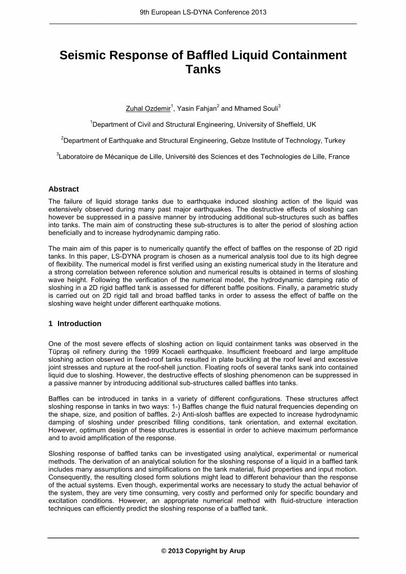
2 Verification of the numerical model

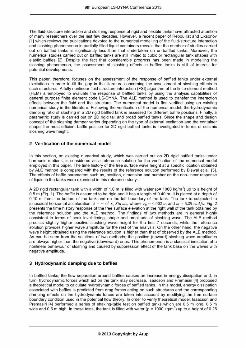
In this section, an existing numerical study, which was carried out on 2D rigid baffled tanks under harmonic motions, is considered as a reference solution for the verification of the numerical model employed in this paper. The time history of the free surface wave height at a specific location obtained by ALE method is compared with the results of the reference solution performed by Biswal et al. [3]. The effects of baffle parameters such as, position, dimension and number on the non-linear response of liquid in the tanks were examined in this reference study. A 2D rigid rectangular tank with a width of 1.0 m is filled with water (ρ= 1000 kg/m3) up to a height of 0.5 m (Fig. 1). The baffle is assumed to be rigid and it has a length of 0.40 m. It is placed at a depth of 0.10 m from the bottom of the tank and on the left boundary of the tank. The tank is subjected to sinusoidal horizontal acceleration, , where and . Fig. 2 presents the time history response of the free surface elevation at the right wall of the tank obtained by the reference solution and the ALE method. The findings of two methods are in general highly consistent in terms of peak level timing, shape and amplitude of sloshing wave. The ALE method predicts slightly higher positive sloshing wave height for the first 7 seconds, while the reference solution provides higher wave amplitude for the rest of the analysis. On the other hand, the negative wave height obtained using the reference solution is higher than that of observed by the ALE method. As can be seen from the solutions of two methods, the positive (upward) sloshing wave amplitudes are always higher than the negative (downward) ones. This phenomenon is a classical indication of a nonlinear behaviour of sloshing and caused by suppression effect of the tank base on the waves with negative amplitude.

3 Hydrodynamic damping due to baffles

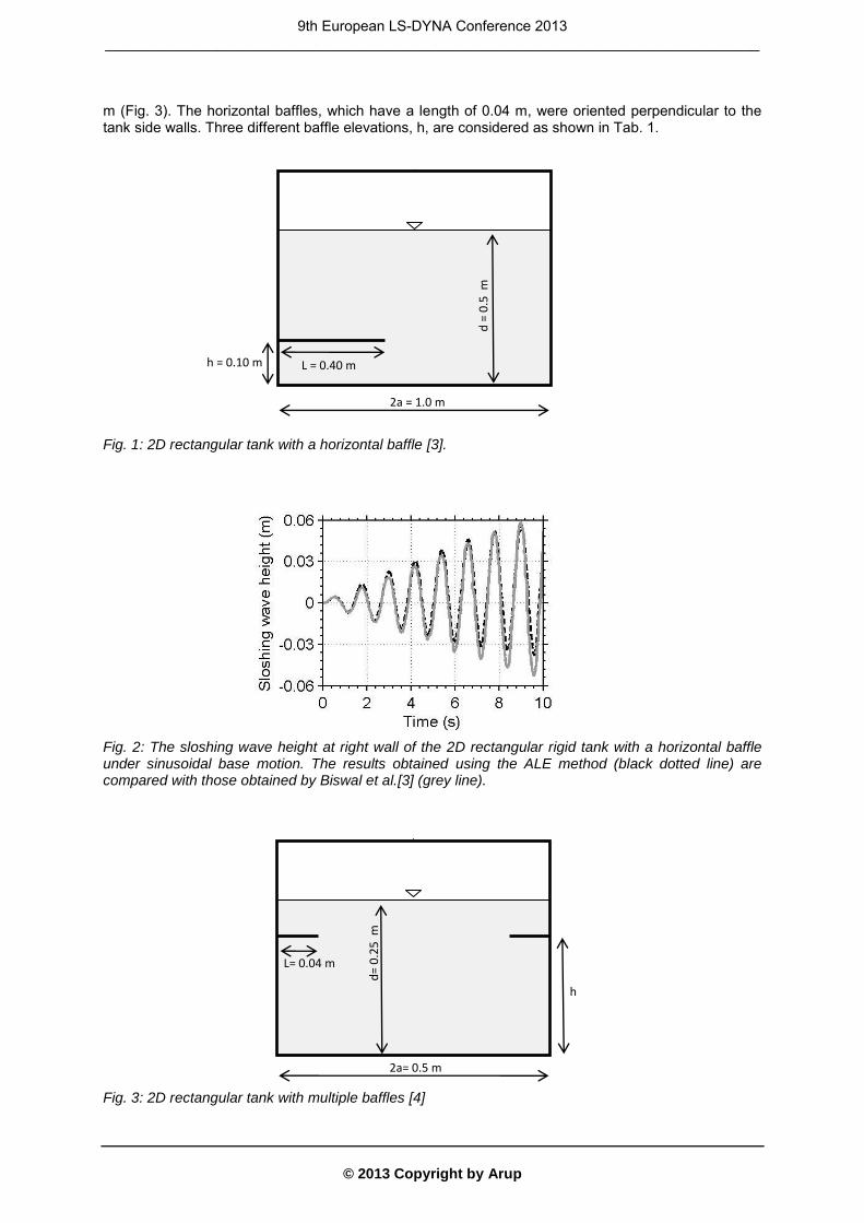
In baffled tanks, the flow separation around baffles causes an increase in energy dissipation and, in turn, hydrodynamic forces which act on the tank may decrease. Isaacson and Premasiri [4] proposed a theoretical model to calculate hydrodynamic forces of baffled tanks. In this model, energy dissipation associated with baffles is predicted from drag forces acting on such structures and the corresponding damping effects on the hydrodynamic forces are taken into account by modifying the free surface boundary condition used in the potential flow theory. In order to verify theoretical model, Isaacson and Premasiri [4] performed a series of shaking-table test on baffled tanks which are 0.5 m long, 0.5 m wide and 0.5 m high. In these tests, the tank is filled with water (ρ = 1000 kg/m3) up to a height of 0.25



m (Fig. 3). The horizontal baffles, which have a length of 0.04 m, were oriented perpendicular to the tank side walls. Three different baffle elevations, h, are considered as shown in Tab. 1.

Fig. 1: 2D rectangular tank with a horizontal baffle [3].

Fig. 2: The sloshing wave height at right wall of the 2D rectangular rigid tank with a horizontal baffle under sinusoidal base motion. The results obtained using the ALE method (black dotted line) are compared with those obtained by Biswal et al.[3] (grey line).

Fig. 3: 2D rectangular tank with multiple baffles [4]

2a= 0.5 m

L= 0.04 m d

= 0

.25

m

h

2a = 1.0 m

L = 0.40 m

d =

0.5

m

h = 0.10 m m



Tab. 1: Tank dimensions [4]

The hydrodynamic sloshing damping ratio can be determined experimentally in time domain from the free vibration response of sloshing using the logarithmic decrement method. In this method, tank is forced using a harmonic motion with a frequency equal to its corresponding fundamental sloshing frequency until reaching a steady state or enough large free surface displacement. Then, the oscillation is quickly stopped and the decay rate of the free surface displacement is recorded. Logarithmic decrement, which is the natural logarithmic value of the ratio of peak values of displacement, can be used to obtain sloshing damping ratio [5]:

where, Di and Di+n are the sloshing amplitudes measured in i and i +n oscillation cycles. In the current study, the logarithmic decrement method is employed to compute sloshing damping in the 2D rigid baffled tanks and results compared with the results of theoretical and experimental works of Isaacson and Premasiri [4]. In the numerical model, element size is considered as 0.025 m for the ALE fluid elements and the tank mesh. The amplitude of the sinusoidal harmonic motion is considered as 0.01 m. The circular frequencies of the harmonic motion are obtained using sloshing frequencies:

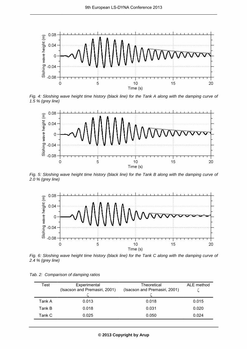
where g is gravitational acceleration and n represents mode number. The sloshing wave height time histories for different baffle positions obtained using the ALE method are shown in Figures 4, 5 and 6. In addition, damping curves are also superimposed in these figures. The sloshing damping ratio using the logarithmic decrement method can be obtained in many different ways. Any two consecutive oscillation cycles which occur following the end of motion can be used in Equation (1). As an alternative, the amplitude of non-sequential peaks can also be used in Equation 1 in order to calculate the damping ratio. Therefore, these various different alternatives can give a variety of sloshing damping ratios. In this work, a mean damping ratio is obtained by taking an average from a number of damping ratios of different sequential peaks and this average damping value is represented by a damping curve (grey line) in Figures 4, 5 and 6. Each of these damping curves represents an average damping ratio for each sloshing wave height time history. In Tab. 2, the hydrodynamic sloshing damping ratios obtained using the ALE method is compared with the theoretical and experimental damping ratios predicted by Isacson and Premasiri [4]. As can be seen from this table, although theoretical model deviates from the experimental findings, the ALE method can predict experimental damping ratios with high accuracy. Seismic tank design codes [6, 7] specify a damping ratio of 0.5 % for the sloshing action of the contained liquid. Tab. 1 also shows that the sloshing damping ratio of baffled tanks is around 1- 2%. Therefore, baffles are effective at increasing slohing damping. However, an extensive study is necessary to assess the effect of position and size of baffles on the seismic response of tanks. Therefore, next section is devoted to a parametric study of sloshing response of baffled tanks under earthquake motions.

Test h/d h (m)

Tank A 0.6 0.15 Tank B 0.7 0.175 Tank C 0.8 0.20

(1)

(2)



Fig. 4: Sloshing wave height time history (black line) for the Tank A along with the damping curve of 1.5 % (grey line)

Fig. 5: Sloshing wave height time history (black line) for the Tank B along with the damping curve of 2.0 % (grey line)

Fig. 6: Sloshing wave height time history (black line) for the Tank C along with the damping curve of 2.4 % (grey line) Tab. 2: Comparison of damping ratios

Test Experimental

(Isacson and Premasiri, 2001)

Theoretical (Isacson and Premasiri, 2001)

ALE method

Tank A 0.013 0.018 0.015

Tank B 0.018 0.031 0.020

Tank C 0.025 0.050 0.024



4 Seismic response of 2D rigid baffled tanks

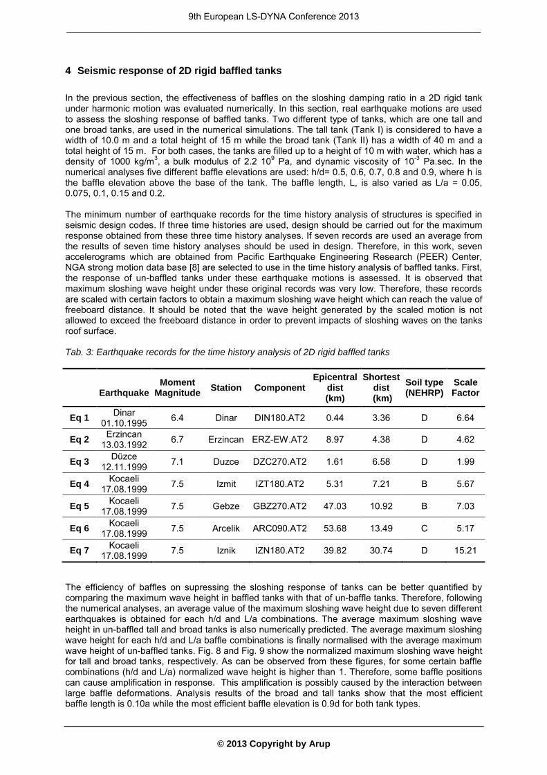
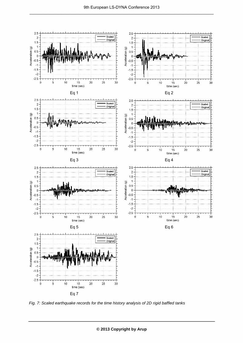
In the previous section, the effectiveness of baffles on the sloshing damping ratio in a 2D rigid tank under harmonic motion was evaluated numerically. In this section, real earthquake motions are used to assess the sloshing response of baffled tanks. Two different type of tanks, which are one tall and one broad tanks, are used in the numerical simulations. The tall tank (Tank I) is considered to have a width of 10.0 m and a total height of 15 m while the broad tank (Tank II) has a width of 40 m and a total height of 15 m. For both cases, the tanks are filled up to a height of 10 m with water, which has a density of 1000 kg/m3, a bulk modulus of 2.2 109 Pa, and dynamic viscosity of 10-3 Pa.sec. In the numerical analyses five different baffle elevations are used: h/d= 0.5, 0.6, 0.7, 0.8 and 0.9, where h is the baffle elevation above the base of the tank. The baffle length, L, is also varied as L/a = 0.05, 0.075, 0.1, 0.15 and 0.2. The minimum number of earthquake records for the time history analysis of structures is specified in seismic design codes. If three time histories are used, design should be carried out for the maximum response obtained from these three time history analyses. If seven records are used an average from the results of seven time history analyses should be used in design. Therefore, in this work, seven accelerograms which are obtained from Pacific Earthquake Engineering Research (PEER) Center, NGA strong motion data base [8] are selected to use in the time history analysis of baffled tanks. First, the response of un-baffled tanks under these earthquake motions is assessed. It is observed that maximum sloshing wave height under these original records was very low. Therefore, these records are scaled with certain factors to obtain a maximum sloshing wave height which can reach the value of freeboard distance. It should be noted that the wave height generated by the scaled motion is not allowed to exceed the freeboard distance in order to prevent impacts of sloshing waves on the tanks roof surface. Tab. 3: Earthquake records for the time history analysis of 2D rigid baffled tanks

Earthquake Moment

Magnitude Station Component

Epicentral dist (km)

Shortest dist

(km)

Soil type (NEHRP)

Scale Factor

Eq 1 Dinar

01.10.1995 6.4 Dinar DIN180.AT2 0.44 3.36 D 6.64

Eq 2 Erzincan

13.03.1992 6.7 Erzincan ERZ-EW.AT2 8.97 4.38 D 4.62

Eq 3 Düzce

12.11.1999 7.1 Duzce DZC270.AT2 1.61 6.58 D 1.99

Eq 4 Kocaeli

17.08.1999 7.5 Izmit IZT180.AT2 5.31 7.21 B 5.67

Eq 5 Kocaeli

17.08.1999 7.5 Gebze GBZ270.AT2 47.03 10.92 B 7.03

Eq 6 Kocaeli

17.08.1999 7.5 Arcelik ARC090.AT2 53.68 13.49 C 5.17

Eq 7 Kocaeli

17.08.1999 7.5 Iznik IZN180.AT2 39.82 30.74 D 15.21

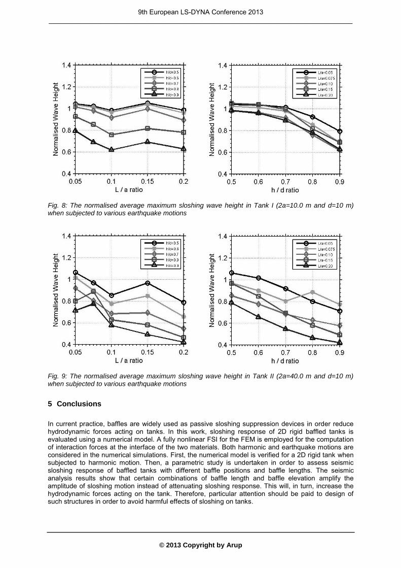
The efficiency of baffles on supressing the sloshing response of tanks can be better quantified by comparing the maximum wave height in baffled tanks with that of un-baffle tanks. Therefore, following the numerical analyses, an average value of the maximum sloshing wave height due to seven different earthquakes is obtained for each h/d and L/a combinations. The average maximum sloshing wave height in un-baffled tall and broad tanks is also numerically predicted. The average maximum sloshing wave height for each h/d and L/a baffle combinations is finally normalised with the average maximum wave height of un-baffled tanks. Fig. 8 and Fig. 9 show the normalized maximum sloshing wave height for tall and broad tanks, respectively. As can be observed from these figures, for some certain baffle combinations (h/d and L/a) normalized wave height is higher than 1. Therefore, some baffle positions can cause amplification in response. This amplification is possibly caused by the interaction between large baffle deformations. Analysis results of the broad and tall tanks show that the most efficient baffle length is 0.10a while the most efficient baffle elevation is 0.9d for both tank types.



Eq 1 Eq 2

Eq 3 Eq 4

Eq 5 Eq 6

Eq 7 Fig. 7: Scaled earthquake records for the time history analysis of 2D rigid baffled tanks



Fig. 8: The normalised average maximum sloshing wave height in Tank I (2a=10.0 m and d=10 m) when subjected to various earthquake motions

Fig. 9: The normalised average maximum sloshing wave height in Tank II (2a=40.0 m and d=10 m) when subjected to various earthquake motions

5 Conclusions

In current practice, baffles are widely used as passive sloshing suppression devices in order reduce hydrodynamic forces acting on tanks. In this work, sloshing response of 2D rigid baffled tanks is evaluated using a numerical model. A fully nonlinear FSI for the FEM is employed for the computation of interaction forces at the interface of the two materials. Both harmonic and earthquake motions are considered in the numerical simulations. First, the numerical model is verified for a 2D rigid tank when subjected to harmonic motion. Then, a parametric study is undertaken in order to assess seismic sloshing response of baffled tanks with different baffle positions and baffle lengths. The seismic analysis results show that certain combinations of baffle length and baffle elevation amplify the amplitude of sloshing motion instead of attenuating sloshing response. This will, in turn, increase the hydrodynamic forces acting on the tank. Therefore, particular attention should be paid to design of such structures in order to avoid harmful effects of sloshing on tanks.



6 References

[1] Rebouillat S. ve D. Liksonov, Fluid–Structure Interaction in Partially Filled Liquid Containers: A Comparative Review of Numerical Approaches, Computers and Fluids, 39, 739-746, (2010).

[2] Eswaran M., Saha U.K. ve Maity D., Effect of baffles on a partially filled cubic tank: numerical

simulation and experimental validation, Computers and Structures 87, 198–205, (2009). [3] Biswal, K. C., Bhattacharyya, S. K. and Sinha, P. K., Non-linear sloshing in partially liquid filled

containers with baffles, International Journal for Numerical Methods in Engineering 68, 3,317–337, (2006).

[4] Isaacson, M. and Premasiri, S., Hydrodynamic damping due to baffles in a rectangular tank,

Canadian Journal of Civil Engineers 28, 608–616, (2001). [5] Chopra, A. K., Dynamics of Structures: Theory and Applications to Earthquake Engineering,

Prentice-Hall, Englewood Cliffs, NJ, (1995). [6] API 650, Welded Storage Tanks for Oil Storage, American Petroleum Institute Standard,

Washington D. C., ( 2003). [7] Eurocode 8, Design of Structures for Earthquake Resistance, Part 4-Silos, Tanks and Pipelines,

European Committee for Standardization, Brussels, BS EN 1998-4, (2006). [8] Pacific Earthquake Engineering Research (PEER) Center, PEER Strong Motion Database,

http://peer.berkeley.edu/smcat/, (2006).


Documents

FEA Information Engineering Journal Information Engineering Journal February 2014.pdf · FEA Information Engineering Journal (FEAIEJ™) is a monthly published online journal to cover