Embed Size (px)
Citation preview
FEASIBILITY OF USING CLASSIFICATION ANALYSES TO DETERMINE
TROPICAL CYCLONE RAPID INTENSIFICATION
THESIS
Jonathan W. Leffler, Captain, USAF
AFIT/GM/ENP/04-07
DEPARTMENT OF THE AIR FORCE AIR UNIVERSITY
AIR FORCE INSTITUTE OF TECHNOLOGY
Wright-Patterson Air Force Base, Ohio
APPROVED FOR PUBLIC RELEASE; DISTRIBUTION UNLIMITED.

The views expressed in this thesis are those of the author and do not reflect the official policy or position of the United States Air Force, Department of Defense, or the United States Government.

AFIT/GM/ENP/04-07
FEASIBILITY OF USING CLASSIFICATION ANALYSES TO DETERMINE TROPICAL CYCLONE RAPID INTENSIFICATION
THESIS
Presented to the Faculty
Department of Engineering Physics
Graduate School of Engineering and Management
Air Force Institute of Technology
Air University
Air Education and Training Command
In Partial Fulfillment of the Requirements for the
Degree of Master of Science in Meteorology
Jonathan W. Leffler, BS
Captain, USAF
March 2004
APPROVED FOR PUBLIC RELEASE; DISTRIBUTION UNLIMITED.

AFIT/GM/ENP/04-07
FEASIBILITY OF USING CLASSIFICATION ANALYSES TO DETERMINE TROPICAL CYCLONE RAPID INTENSIFICATION
Jonathan W. Leffler, BS
Captain, USAF
Approved:

iv
AFIT/GM/ENP/04-07
Abstract
Tropical cyclone intensity techniques developed by Dvorak have thus far been
regarded by tropical meteorologists as the best identification and forecast schemes
available using satellite imagery. However, in recent years, several ideologies have
arisen which discuss alternative means of determining typhoon rapid intensification or
weakening in the Pacific. These theories include examining channel outflow patterns,
potential vorticity superposition and anomalies, tropical upper tropospheric trough
interactions, environmental influences, and upper tropospheric flow transitions.
It is now possible to data mine these atmospheric parameters thought partly
responsible for typhoon rapid intensification and weakening to validate their usefulness
in the forecast process. Using the latest data mining software tools, this study used
components of NOGAPS analyses along with selected atmospheric and climatological
predictors in classification analyses to create conditional forecast decision trees. The
results of the classification model show an approximate R2 of 0.68 with percent error
misclassifications of 13.5% for rapidly weakening typhoon events and 21.8% for rapidly
intensifying typhoon events. In addition, a merged set of suggested forecast splitting
rules was developed. By using the three most accurate predictors from both intensifying
and weakening storms, the results validate the notion that multiple parameters are
responsible for rapid changes in typhoon development.

v
Acknowledgements
There are many people whom I would like to thank on this project. First and
foremost, I thank the Lord for giving me wisdom to complete the research, humility to
keep trying, and patience to work with outcomes, which had not been foreseen. I would
also like to thank my advisor, Lt Col Ron Lowther, and my other committee members, Lt
Col Michael Walters and Professor Dan Reynolds, for their insight and willingness to
help me when I was unable to see the road ahead. I am also truly indebted to my
wonderful wife and brand new daughter for the hundreds of hours I’ve spent locked up in
an office or away from home. Thank you for your understanding and loyalty.
This thesis work would not have been accomplished without the help of Capt
Steve Vilpors of the Joint Typhoon Warning Center and Jeff Zautner of the Air Force
Combat Climatology Center. Thank you both for answering all my questions and
providing the data for this study. In addition, I would like to thank Mikhail Golovnya of
Salford Systems, Inc., who persisted in helping me master concepts of the CART data
mining software. Finally, to my classmates who have supported me from the beginning,
thank you for your teamwork and your knowledge during these past 18 months. It has
definitely been an experience I will always remember.
Jonathan W. Leffler

vi
Table of Contents
Abstract ............................................................................................................................. iv
Acknowledgements ............................................................................................................ v
List of Figures ................................................................................................................. viii
List of Tables ..................................................................................................................... x
I. Introduction .................................................................................................................... 1
1.1 Statement of the Problem .......................................................................................... 2 1.2 Research Objectives .................................................................................................. 3 1.3 Research Approach ................................................................................................... 7
II. Literature Review .......................................................................................................... 9
2.1 Dvorak Technique ..................................................................................................... 9 2.2 Channel Outflow Patterns and Opposite Hemisphere Effects ................................ 14 2.3 Potential Vorticity Superposition and Anomalies ................................................... 17 2.4 Tropical Upper Tropospheric Trough Interactions ................................................. 19 2.5 Environmental Influences ....................................................................................... 23 2.5.1 Sea Surface Temperatures .............................................................................. 23 2.5.2 Effects of Vertical Shear ................................................................................ 24 2.5.3 Air Sea Interactions ........................................................................................ 27 2.6 Upper Tropospheric Flow Transitions .................................................................... 28
III. Methodology .............................................................................................................. 30
3.1 Introduction ............................................................................................................. 30 3.2 Data Acquisition ..................................................................................................... 30 3.2.1 Storm Selection .............................................................................................. 30 3.2.2 Best Track Data .............................................................................................. 31 3.2.3 NOGAPS Model ............................................................................................ 32 3.2.4 Sea Surface Temperatures .............................................................................. 34 3.2.5 CPC Teleconnection Indices .......................................................................... 35 3.3 CART Overview ..................................................................................................... 36 3.3.1 Methods .......................................................................................................... 38 3.3.1.1 Tree Splitting Methods ...................................................................... 38 3.3.1.2 Pruning ............................................................................................... 41 3.3.1.3 Cross Validation ................................................................................. 42 3.3.1.4 Improvement Scores .......................................................................... 43

vii
3.3.1.5 Class Assignments ............................................................................. 44 3.3.2 Research Predictors ........................................................................................ 45 3.4 Statistical Overview ................................................................................................ 49 3.4.1 Introduction .................................................................................................... 49 3.4.2 Simple Linear Regression .............................................................................. 50
IV. Analysis and Results .................................................................................................. 53
4.1 Introduction ............................................................................................................. 53 4.2 Regression Analysis of NOGAPS and Best Track Data ......................................... 53 4.3 Classification Tree Analysis ................................................................................... 55 4.3.1 Best Method Determination ........................................................................... 55 4.3.2 Alternate Target Classification Tree Results ................................................. 62 4.3.3 Primary Target Classification Tree Results ................................................... 65 4.4 Supplement to the Intensity Analysis Worksheet and Verification ........................ 78
V. Conclusions and Recommendations ........................................................................... 83
5.1 Conclusions ............................................................................................................. 83 5.2 Recommendations ................................................................................................... 86 5.2.1 Recommendations to JTWC .......................................................................... 86 5.2.2 Future Research Recommendations ............................................................... 88
Appendix A: MATLAB Linear Interpolation of Grid Points Program ........................... 90
Appendix B: MATLAB Calculation of Wind Shear Program ......................................... 92
Appendix C: Complete Set of Splitting Rules ................................................................. 98
Acronyms ....................................................................................................................... 102
Bibliography .................................................................................................................. 104
Vita ................................................................................................................................. 108
viii
List of Figures
Figure Page 1. Intensity change curves of the model ........................................................................... 10
2. Common TC patterns and corresponding T-numbers .................................................. 11
3. Examples of TC Patterns ............................................................................................. 11
4. Example of a LOG10 spiral graph ............................................................................... 12
5. Corresponding LOG10 spiral graph reference ............................................................. 12
6. Variety of outflow patterns associated with TC intensification for Northern Hemisphere cases.......................................................................................................... 15
7. Six types of interactions between a TC and its surroundings ...................................... 21
8. 1997 Northwest Pacific TC tracks ............................................................................... 25
9. 1999 Northwest Pacific TC tracks ............................................................................... 26
10. 2001 Northwest Pacific TC tracks ............................................................................. 26
11. Sample Gini splitting function ................................................................................... 39
12. Sample Twoing splitting function .............................................................................. 39
13. Graphical depiction of 10-fold cross validation ......................................................... 43
14. Example of an improvement score ............................................................................ 44
15. Classification tree for CAT STSS .............................................................................. 63
16. Classification tree for CAT STDS ............................................................................. 63
17. Classification tree for TGT (Class 2).......................................................................... 66
18. Classification tree for TGT (Class 1).......................................................................... 66
19. Classification tree for TGT (Class 0).......................................................................... 67
20. New classification tree for TGT (Class 2) ................................................................. 70

ix
21. New classification tree for TGT (Class 1) ................................................................. 70
22. New classification tree for TGT (Class 0) ................................................................. 71
23. Splitters for new classification tree............................................................................. 71
24. JMP distribution of Class 1......................................................................................... 75
25. JMP distribution of Class 2......................................................................................... 75
x
List of Tables
Table Page 1. Empirical relationship between CI number and MWS, and the relationship between the T-number and MSLP ............................................................................... 14
2. Selected typhoons from 1997, 1999, and 2001 ............................................................ 31
3. Sample best track data for TC 04 ................................................................................. 32
4. NOGAPS model fields ................................................................................................. 33
5. Storms with missing model fields ................................................................................ 34
6. List of CART predictors .............................................................................................. 46
7. Rules for categorical predictors ................................................................................... 47
8. Categorical values for predictor rules .......................................................................... 47
9. Initial regression analysis of NOGAPS and BT .......................................................... 55
10. Initial screening of relative cost ................................................................................. 56
11. Initial screening of percent error misclassification .................................................... 56
12. Initial screening of percent prediction success .......................................................... 57
13. Total counts of initial screening ................................................................................. 59
14. Average percent error misclassification ..................................................................... 59
15. Percent error misclassification for CAT STSS .......................................................... 61
16. Percent error misclassification for CAT STDS ......................................................... 61
17. Percent error misclassification for CH OUT ............................................................. 62
18. Terminal node details for CAT STSS......................................................................... 63
19. Terminal node details for CAT STDS ....................................................................... 63
20. Splitting rules for CAT STSS .................................................................................... 64

xi
21. Splitting rules for CAT STDS .................................................................................... 64
22. Terminal node details for TGT .................................................................................. 67
23. Variable importance for TGT .................................................................................... 69
24. Refined variable importance for TGT ........................................................................ 69
25. New terminal node details for TGT ........................................................................... 73
26. Class 1 and Class 2 splitting rules .............................................................................. 74
27. JMP moments table for class distributions ................................................................ 74
28. Criteria used to determine validity of splitting rules ................................................. 77
29. TC intensity analysis worksheet ................................................................................ 80
30. Suggested forecast splitting rules ............................................................................... 80
31. Verification counts of the forecast splitting rules ...................................................... 81
32. Accuracy of the forecast splitting rules ..................................................................... 81

1
FEASIBILITY OF USING CLASSIFICATION ANALYSES TO DETERMINE TROPICAL CYCLONE RAPID INTENSIFICATION
I. Introduction
For the past 45 years, the Joint Typhoon Warning Center (JTWC), currently
located in Hawaii, has been responsible for the observation, analysis, forecast, and public
dissemination of tropical cyclone warnings in the western and southern Pacific and Indian
Ocean basins. During this time, numerous tropical cyclones have impacted Department
of Defense assets, stretching from Hawaii to Japan. A tropical cyclone (TC), commonly
known in the western Pacific Ocean as a typhoon, can vary in strength and is categorized
according to its maximum wind speeds. A tropical depression (TD) is defined by winds
< 17 m s-1, a tropical storm (TS) is defined by winds 18 to 32 m s-1, and a typhoon is
defined by winds > 33 m s-1. There is also a special category of TC called super typhoon,
which requires winds > 65 m s-1. This is comparable to a Category IV+ hurricane on the
Saffir-Simpson hurricane scale (Glickman et al. 2000).
During the past decade, the precision of typhoon forecast tracks has improved
greatly, thanks to the help of advances in numerical modeling, such as the Systematic
Approach to Tropical Cyclone Forecasting Aid (SAFA) program, and computer systems
such as the Automated Tropical Cyclone Forecasting (ATCF) system (Vilpors personal
correspondence 2003). However, one of the main concerns of JTWC has been the ability
to accurately predict intensity changes of tropical cyclones in advance.

2
“In the early days of meteorological satellite programs, the feasibility of using
satellite imagery for tropical cyclone analysis was recognized” (Sadler 1964). In 1973,
Vernon Dvorak developed a technique by which intensification could be predicted based
on the current configuration of cloud features (Dvorak 1974). JTWC has been using this
method as its main technique to analyze current and forecast intensity factors. However,
during the past few years, several researchers have proposed other means of forecasting
tropical cyclone intensification. Some of these proposals include using channel outflow
patterns, potential vorticity superposition and anomalies, tropical upper tropospheric
trough (TUTT) interaction, environmental influences, and upper tropospheric flow
transitions. The following chapters explore these inner workings of tropical cyclone
intensification.
1.1 Statement of the Problem
The Joint Typhoon Warning Center has become relatively proficient in
forecasting the movement of tropical cyclones. However, they lack substantial expertise
in predicting tropical cyclone intensification. Specifically, they have requested tools for
tropical cyclone intensity forecasting using synoptic patterns defined by water vapor
imagery, observations, and model field analyses. JTWC also requested a guideline for
slow, climatological and rapid deepeners to include the effects of tropical upper
tropospheric trough cells on intensification trends. The current procedure for forecasting
intensification has been the Dvorak Technique, from which the T-number is computed.
The T-number is simply a numeric designator for the current intensity of a tropical

3
cyclone. For a slowly intensifying tropical cyclone, the T-number rises 0.5 per day; a
steady or climatologically intensifying cyclone increases at 1.0 T-number per day; and a
rapidly intensifying system rises 1.5 T-number or more per day.
Although this technique is considered quite accurate, it can be highly subjective
depending on the lifecycle of the tropical cyclone and how well its central and banding
features are defined. The overall premise of the technique relies on cloud pattern
recognition and comparison with a model of anticipated intensity trends. The technique
does not take TUTT cell interactions into account, therefore alternative methods must be
devised.
1.2 Research Objectives
The overall goal of this thesis is to data mine atmospheric parameters responsible
for typhoon rapid intensification and weakening and to validate the usefulness of using
these parameters in the forecast process. This thesis examines a variety of mechanisms
thought responsible for tropical cyclone intensification. Chapter 2 discusses these
parameters individually, exploring the inner workings of tropical cyclone intensification,
and illustrating relationships between the different parameters. Chapter 3 portrays the
methodology involved in this research, from selection of typhoons and predictors to a
quick overview of simple linear regression. Chapter 4 is devoted to analysis and results
while Chapter 5 yields conclusions to this thesis and recommendations for future work.
The first objective of this research is to gather all types of satellite imagery
(visible, water vapor, and infrared) since satellite interrogation is one of the primary tools

4
in analyzing Northwest Pacific typhoons. This imagery is archived by the Naval
Research Laboratory (NRL), according to each typhoon event, as well as by the
Australian Bureau of Meteorology (BOM). In addition, the imagery should include the
entire lifetime of the tropical cyclone, if possible, from tropical depression to typhoon
strength. Still satellite imagery is used in the analysis, however animation loops are also
beneficial in order to show changes over time. Although emphasis has been placed on
water vapor imagery (given that this particular channel depicts the upper portions of the
atmosphere), visible and infrared imagery are not excluded due to their unique
perspective of the events. Visible imagery can show both upper and lower level cloud
fields (inflows, outflows, and convective activity), whereas infrared imagery can isolate
the typhoon core when the eye is obscured by cloud cover. Infrared imagery can also
show areas of enhanced convection due to colder cloud tops. This knowledge proves
very useful in determining whether a typhoon is gaining or losing strength.
The second objective of the research is to collect the best track data from JTWC.
The best track data are reanalyses of every typhoon event during the year in each of the
ocean basins. These data include six hourly fixes on each storm to include latitude,
longitude, maximum sustained wind speed (kts), and minimum sea level pressure (mb).
Best track data serve as the official record of the typhoon’s progress, both in intensity
changes and movement. This information is absolutely essential since it provides the
closest ground truth for any analysis and a basis from which to build a forecasting
methodology. Several graphical depictions are developed from the best track data in
order to provide a quick look at key timeframes in typhoon lifecycles. Also, the different

5
mechanisms which cause increases or decreases in central surface pressure can be
compared to determine any relationships which prove helpful during analysis.
A third objective is to collect the Navy Operational Global Atmospheric
Prediction System (NOGAPS) model field analyses. NOGAPS is the preferred model in
this analysis because its global domain includes the Pacific basin, and it is available from
the Fleet Numerical Meteorology and Oceanography (FLENUMMETOC) Detachment at
the Air Force Combat Climatology Center (AFCCC) for the 1997, 1999, and 2001
typhoon seasons. These years are selected due to climatological importance, discussed in
the fourth objective. The National Centers for Environmental Prediction (NCEP) also
archive model fields such as temperature, pressure, etc. which are available for
reanalysis. These fields are a vital link to the research because the entire area of interest
is open ocean, and there are no surface based observations from which to draw data.
Also, the usage of routine upper air soundings is limited, therefore model fields become
the dominant analysis tool. In addition, there are no longer aircraft reconnaissance flights
such as those which currently exist over the Atlantic basin. Hence all of the available
fields (temperature, pressure, moisture, winds, etc.) are necessary components in the data
set, given the aforementioned constraints. Some of the proposed mechanisms for
intensification rely on derived model fields (potential vorticity, etc.), and those
parameters are obtained as well, if they are easily computed or archived.
The fourth objective of the research is to incorporate climatological and
teleconnection indices into the data set for predictive analyses. Climatological conditions
such as El Niño (EN) and La Niña (LN) periods are included to see what effects they
contribute to tropical cyclone intensification. EN and LN events profoundly alter
6
tropospheric circulation in the western North Pacific. “Alteration of vertical shear causes
tropical cyclones to form farther south and east than normal during EN events, and
farther north and west than normal during LN events” (Ford 2000). Sea surface
temperature patterns are also a major factor in determining TC development areas.
“These formation site differences lead to longer tracks and stronger tropical cyclones
during EN, and shorter tracks and weaker tropical cyclones during LN events” (Ford
2000). Recent EN years include 1994-95 and 1997-98, while recent LN years include
1996-97 and 1998-99. In order to manage the amount of typhoon data and compare with
the availability of NOGAPS and National Climatic Data Center (NCDC) model fields,
1997 is selected as the EN year and 1999 as the LN year for this analysis. In contrast,
2001 is selected as a neutral (NU) year, where neither EN nor LN regimes dominated.
The fifth objective of the research is to examine relationships between the
proposed intensification mechanisms, which is done via classification and regression tree
(CART) analyses. CART is the backbone of the research because the main goal rests on
using a variety of predictors to determine typhoon intensity trends. Other researchers
have already shown that several mechanisms result in the intensification or dissipation of
the storms (Chen and Gray 1985, Davidson and Kar 2002, DeMaria 1996, Evans 1993,
Hanley et al. 2001, Holland 1997, Merrill 1987, Molinari et al. 1998, Sadler 1975, Sadler
1978, Sikora et al. 1976). If a pattern of intensification exists among different
atmospheric parameters, then understanding this pattern will help JTWC improve its
intensity forecasts. Using CART software will help isolate patterns in the data. Since no
one parameter is the ultimate factor in strengthening or weakening a typhoon, a synergy

7
between several predictors may be responsible for these rapid changes during the
lifecycle.
1.3 Research Approach
The approach to this research is two fold. First, an objective analysis is
accomplished by gathering archived numerical data such as pressure, wind, sea surface
temperature, wind shear, etc. All of these fields are computed by models or observed by
satellite remote sensing. Second, a subjective analysis is performed to fill in the gaps
where objective analyses are not possible. For example, in examining channel outflow
patterns or TUTT interactions, this determination is a subjective call by the analyst. The
NOGAPS model does not generate a field for outflows nor upper tropospheric
interactions. CART data mining brings these various ideologies of intensification
together.
CART analyses are designed to find patterns in sets of data. Based upon
predetermined conditions, these analyses can map the anticipated trend of an event (i.e.,
they build conditional forecast decision trees). They use various functions and splitting
rules to determine how a tree is developed into subcategories, called nodes. Once a
terminal node is reached, meaning that the data can no longer be split further, conclusions
can be drawn from information contained in different nodes, and a pattern in the data
could be recognized. The splitting process occurs from a set of predictors, defined at the
beginning of the tree, which result in terminal nodes containing a certain percentage of
the data. This particular process is outlined in Chapter 3.

8
One main challenge of the research is to develop a variety of predictors to be
analyzed by CART. Some of these predictors such as potential vorticity anomalies, sea
surface temperatures, and vertical shear are already employed in current numerical
modeling schemes. Other predictors such as channel outflow patterns, TUTT
interactions, and upper tropospheric flow transitions are apparent in satellite imagery;
however, they are not analyzed as specific model fields. Their contributions are mostly
of a synoptic nature and not derived from numerical methods. The key is to determine
how to bridge together a model analysis field with a synoptic depiction while using the
data mining software.
The second main challenge is to study how CART analyzes these relationships
and to compare the outcomes with the trends in the best track data. Each combination of
predictors results in a decision tree. Once the data are analyzed by CART, the different
decision trees are compared, and a recommendation is made based upon which predictors
are found to have the greatest influence on the target (rapid intensification or rapid
weakening). In order to improve the overall forecast process, it is important to enhance
the current consensus forecasting methods by JTWC with the recursive splitting methods
done by CART. Although the data mining will most likely produce non-traditional
results, the interpretation of these results will be one of the elements required to enhance
intensity forecasting techniques.

9
II. Literature Review
2.1 Dvorak Technique
The technique developed by Dvorak has thus far been regarded, by tropical
meteorologists, as the best intensity identification scheme using satellite imagery. Its
overall basis is to compare the tropical cyclone’s current central features (CF) and
banding features (BF) with a model of tropical cyclone development. “The CF are those
which appear within the broad curve of the comma band and either surround or cover the
cloud system center. The BF refer to only that part of the comma cloud band that is
overcast and curves evenly around the CF” (Dvorak 1974). The model depicts a variety
of tropical cyclone intensity changes and describes how the BF and CF change over time
(Dvorak 1974). Given the current characteristics of the CF and BF, a forecaster can
compare the satellite imagery to a matrix of possible curves. These curves are related to
the T-number, which is simply a numeric designator for the current intensity of the
tropical cyclone. For a slowly intensifying tropical cyclone, one would expect the T-
number to rise 0.5 per day; a steady or climatologically intensifying cyclone would
increase 1.0 T-number per day; and a rapidly intensifying system would grow 1.5 T-
number or more per day. Figure 1 shows trends of T-numbers and the associated rates of
intensification.

10
Figure 1. Intensity change curves of the model. The hatched area surrounding the typical curve is used to represent “intensity” as a zone one T-number wide (modified from Dvorak 1974 and used with permission of the American Meteorological Society (AMS)).
Another important typhoon characteristic the forecaster should recognize is the
central dense overcast (CDO). The CDO is defined as the region of dense cloud near the
core of a tropical cyclone (Glickman et al. 2000). The CDO plays an important role
because it helps determine the intensity trend of the tropical cyclone. If the CDO is
initially small, then becomes larger and more circular over time, the cyclone is
intensifying. Once the CDO, CF, and BF have all been taken into account, comparison of
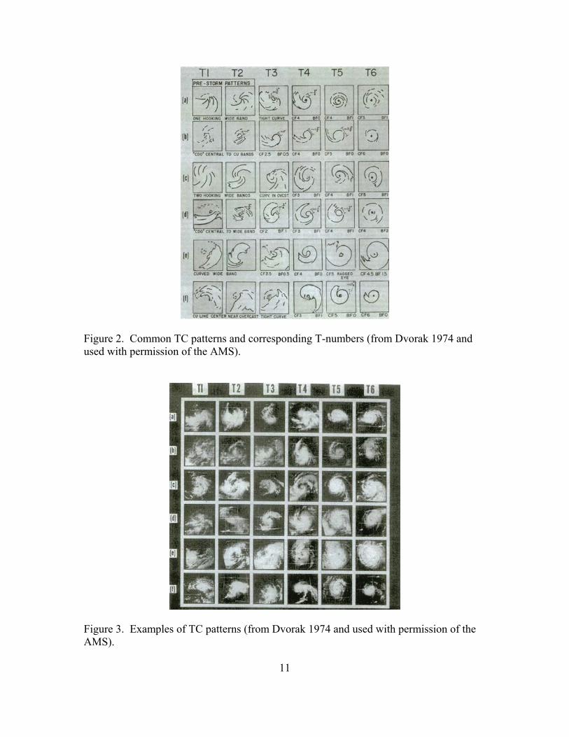
the imagery to the model can be accomplished. Figure 2 shows possible signatures of the
tropical cyclone per designated T-number, and Figure 3 depicts actual images of tropical
cyclones at each level. Note: not all tropical cyclones match exactly to what is depicted
in Figure 2, however an overall “best fit” should be applied.
DAY OF EXPECTED MAX INTENSITY FOR NORTH- WESTWARD MOVING CYCLONES (DAY 4).
FIRST DAY WHEN TODAY’S T-NUMBER IS LESS THAN YESTERDAY’S
11
Figure 2. Common TC patterns and corresponding T-numbers (from Dvorak 1974 and used with permission of the AMS).
Figure 3. Examples of TC patterns (from Dvorak 1974 and used with permission of the AMS).
12
This method, based on pattern recognition, is used when the CDO obscures the
exact center of the cyclone or the low-level cyclonic rotation is not easily identified.
Streamlines can also aid in determining the overall circulation of the TC center. A
second way to calculate the T-number is by using a LOG10 spiral graph.
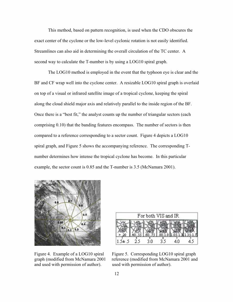
The LOG10 method is employed in the event that the typhoon eye is clear and the
BF and CF wrap well into the cyclone center. A resizable LOG10 spiral graph is overlaid
on top of a visual or infrared satellite image of a tropical cyclone, keeping the spiral
along the cloud shield major axis and relatively parallel to the inside region of the BF.
Once there is a “best fit,” the analyst counts up the number of triangular sectors (each
comprising 0.10) that the banding features encompass. The number of sectors is then
compared to a reference corresponding to a sector count. Figure 4 depicts a LOG10
spiral graph, and Figure 5 shows the accompanying reference. The corresponding T-
number determines how intense the tropical cyclone has become. In this particular
example, the sector count is 0.85 and the T-number is 3.5 (McNamara 2001).
Figure 4. Example of a LOG10 spiral Figure 5. Corresponding LOG10 spiral graph graph (modified from McNamara 2001 reference (modified from McNamara 2001 and and used with permission of author). used with permission of author).

13
The objective of the pattern recognition and LOG10 methods is to compare
today’s imagery with yesterday’s imagery to see how the cloud features have changed. If
there is a good match with the T-number from yesterday’s forecast, then there is high
confidence in future intensification (given current rates of TC growth). If the comparison
is not good based on the new imagery, then the T-number is adjusted for the new
forecast. Finally, the last parameter the forecaster needs to calculate is the current
intensity (CI) number.
“The CI number relates directly to the intensity of the cyclone (in terms of wind
speed) for all typhoon events” (Dvorak 1974). The CI number is the same as the T-
number during development, but remains higher during weakening (McNamara 2001).
This rationale is based on the fact that storm surface vorticity is conserved even though
cloud features are dissipating; the storm still has enough kinetic energy to fuel strong
surface winds (McNamara 2001). Also, the CI number is maintained within < 1.0 of the
T-number during any phase. Table 1 shows the relationship between CI and the
maximum wind speed (MWS) as well as minimum sea level pressure (MSLP).
The current intensity number along with the T-number provides a useful analysis
of current tropical cyclone strength. These parameters are relayed to the public via a
warning bulletin which also maintains continuity of typhoon strength between forecast
shifts. Another useful measure of TC intensification is recognition of channel outflow
patterns.
14
Table 1. Empirical relationship between CI number and MWS, and the relationship between the T-number and MSLP (modified from Dvorak 1974 and used with permission by the AMS).
C.I. Number MWS (knots)
T Number
MSLP (mb) (Atlantic)
MSLP (mb) (NW Pacific)
1.0 25 1.0 1.5 25 1.5 2.0 30 2.0 1009 1003 2.5 35 2.5 1005 999 3.0 45 3.0 1000 994 3.5 55 3.5 994 988 4.0 65 4.0 987 981 4.5 77 4.5 979 973 5.0 90 5.0 970 964 5.5 102 5.5 960 954 6.0 115 6.0 948 942 6.5 127 6.5 935 929 7.0 140 7.0 921 915 7.5 155 7.5 906 900 8.0 170 8.0 890 884
2.2 Channel Outflow Patterns and Opposite Hemisphere Effects
During the year long period of the First Global Atlantic Research Project Global
Experiment (FGGE), Gray and Chen, Colorado State University researchers, studied
upper tropospheric outflow patterns and correlated intensification and weakening based
on those patterns. Intensifying tropical cyclones within the different global ocean basins
typically showed upper level outflow patterns of three basic types: single channel
outflow (S) which included either poleward or equatorward outflow; double channel
outflow (D) in both poleward and equatorial directions; or no channel outflow (N) (Chen
and Gray 1985). Each category of channeling was subcategorized by position of the

15
cyclone center to the outflow. For example, a tropical cyclone centered west of a single
channel poleward outflow would be designated SPW while a tropical cyclone centered
underneath a double outflow channel would be designated DC. Figure 6 shows a matrix
of different cyclone centers and corresponding channels.
Figure 6. Variety of outflow patterns associated with TC intensification for Northern Hemisphere cases (from Chen and Gray 1985 and used with permission of author).
Chen and Gray studied numerous tropical cyclone events, and an analysis of
maximum sustained winds verified the hypotheses of intensification based on outflow
channels. An outflow channel is a narrow region of high speed flow (usually at 200 mb
or approximately 40,000 feet altitude) which evacuates air from the tropical cyclone
center. It is this evacuation of air which allows convection to occur inside of the eyewall
and operates as an exhaust mechanism for continued intensification. Outflow channels
are readily apparent from satellite imagery as long bands of clouds streaking
anticyclonically from the cyclone center. Chen and Gray (1985) found that double
channel outflows were associated with the fastest intensification rates. For single channel

16
patterns, equatorial outflow channels on average lead to faster intensification rates than
poleward channel outflows. Given the variety and location of typhoons within the
database, a comparison was also made between opposite pressure and hemisphere effects
on TC intensification.
Both the location and strength of anticyclones in each hemisphere determined
intensification and weakening via connections with the outflow channels. For example, it
was noted that a strong equatorial upper level anticyclone in the southern hemisphere
(SH) was extremely favorable for enhancing the equatorward outflow of a northern
hemisphere (NH) tropical cyclone and vice versa (Chen and Gray 1985). TD Judy
rapidly intensified into Super Typhoon Judy (maximum winds 135 kts) between 17 and
20 August 1979, due to this positive feedback mechanism. In 1972, rapid deepening of
typhoons Rita, Phyllis, and Tess was “associated with multi-directional outflow channels
to the large-scale flows of the upper troposphere” (Sadler 1978). However, it was also
found that when an upper level SH anticyclone weakened or moved out of proximity to a
NH tropical cyclone, diminishing of the outflow channel would result in steady or rapid
weakening. Sadler (1978) noted these effects with Typhoon Rita, located northwest of
Guam. Between 11 and 14 July 1972, the loss of a strong outflow channel resulted in
rapid filling (910 mb to approximately 965 mb). These examples show how the diversity
of opposite hemisphere anticyclones can strengthen or weaken a typhoon. Although the
literature does not specify the approximate distance from the equator, all of the figures in
the paper suggest anticyclones are located within 15 degrees of the equator for the effect
to occur.

17
Given the validity of these findings, it has become imperative for the forecaster to
monitor cross equatorial effects as well as same hemisphere effects. It is the combination
of a current analysis technique such as Dvorak with an opposite hemisphere relationship
that can dictate future intensity for storms in the vicinity of the equator. However, these
parameters alone should not be regarded as the only measures of intensification. Other
dynamical features, such as potential vorticity, can also explain why a typhoon rapidly
intensifies.
2.3 Potential Vorticity Superposition and Anomalies
Many researchers have argued that the interaction of tropical cyclones with upper-
tropospheric troughs lead to a weakening of the system, whereas others believe this
interaction aids in intensification. In a study conducted on Tropical Cyclone Danny in
1985, Molinari et al. (1998) “maintain that potential vorticity (PV) has become a useful
dynamical framework for examining the interactions of tropical cyclones and upper-
tropospheric vorticity maxima.” In addition, Bluestein (1993) “uses Rossby’s potential
vorticity P:
( )P g fpθθζ ∂= − +
∂ (1)
where
v ux yθ
θ
ζ ∂ ∂= − ∂ ∂ (2)

18
and P is considered potential vorticity.” ζθ is defined as relative vorticity, g is gravity,
and f is the Coriolis parameter. Bluestein (1993) found that for typical midlatitude,
synoptic-scale flow
P gfpθ∂−
∂ (3)
and typically
10100
Kp mbθ∂ −
∂ (4)
where pθ∂
∂ represents the partial derivative of potential temperature with respect to
pressure. Therefore, isentropic potential vorticity is on the order of
( )( )2 4 1 6 2 1 13 2 2
10 110 10 10 110 10
K kPaP m s s m s K kg PVUkPa kg m s m
− − − − − −− −
− − = ≡
(5)
which agrees with the potential vorticity unit (PVU) as defined by Hoskins et al. (1985).
The importance of converting into isentropic potential vorticity (IPV) “thinking” is that
analyses are made easier when working with synoptic-level charts (i.e., orders of
magnitude are diminished). Bluestein (1993) also states that “values less than
approximately 1.5 PVU are usually associated with tropospheric air, while larger IPV
values are typically associated with stratospheric air.” In the study involving TC Danny,
Molinari et al. (1998) found that the cyclone experienced rapid pressure falls as a
relatively small-scale, positive upper potential vorticity anomaly began to superpose with
the low-level center. Although the details of exactly how this interaction worked remains
unclear, it was proposed that a constructive interference process initiated an evaporation-
wind feedback instability (“WISHE” mode; Emanuel 1986). WISHE is a Wind Induced

19
Surface Heat Exchange in which inflow generates evaporation of the water vapor in the
eyewall and releases latent and sensible heat to the system.
Given the complex dynamics of IPV, Bluestein (1993), Thorpe (1986), and
Hoskins et al. (1985) found that the wind field or components of the wind field could be
computed based on the distribution of IPV. Therefore, if large values of upper-level IPV
were superposed with a surface tropical cyclone, the effects would be similar to those of
large values of wind shear. The tropical cyclone would not intensify and/or would
weaken because of the unfavorable conditions (see discussion in Section 2.5.2). The
optimal state for intensification occurs as the tropical cyclone interlocks with small
values of IPV. A small superposition provides enough shear for development but not too
much which would separate the upper and lower cyclone structure. This rationale agrees
with the hypothesis of Molinari et al. (1998) given the relationship between upper level
troughs and upper level vorticity maxima. The upper level trough can also be examined
in terms of the tropical upper tropospheric trough, which is another mechanism of
typhoon intensification.
2.4 Tropical Upper Tropospheric Trough Interactions
The TUTT is defined as “A semi permanent trough extending east-northeast to
west-southwest from about 35°N in the eastern Pacific to about 15°-20°N in the central
west Pacific” (Glickman et al. 2000). Sadler (1975) found that the TUTTs “appear in
summer monthly averaged maps of upper-tropospheric flow over the oceans.” Therefore,
for most practical purposes, tropical cyclone intensification should be at its maximum

20
extent between June and September. Many studies have been accomplished and
determined that it is the interaction with this trough (or series of cold lows) which aids in
the intensification of tropical cyclones. Similar to the interactions of PV anomalies, the
origin of the TUTT remains somewhat of a mystery, given that it is not a permanent
feature.
Ferreira and Schubert (1999) have noted that “in water vapor images and upper-
level IPV plots, TUTT cells appear as dry regions (dark in the water vapor imagery) of
intense cyclonic PV.” They propose that TUTT cells originate as extrusions of
midlatitude stratospheric air into the tropics. This proposition agrees with the PV
research by Molinari et al. (1998). Observational studies by Kelley and Mock (1982),
Whitfield and Lyons (1992), and Price and Vaughan (1992), found that “TUTT cells are
cold core cyclones whose typical horizontal scale is on the order of several hundred
kilometers. They also found that TUTT cells typically last for less than five days but
may, in some cases, persist for nearly two weeks.” An important relationship between
TUTT cells and tropical cyclone intensification has been proximity to each other.
Previously, it was stated that an optimal distance to the TUTT existed for
typhoons to intensify (given small values of IPV). This relationship also holds true for
the horizontal distance to upper cyclones. The upper cyclone (UC) is generally observed
at the 200 to 250 mb level, and Sadler (1978) found that, in particular, north to northwest
of the tropical cyclone is the optimal position of the UC for efficient mass and heat
evacuation. This process allows the outflow channel access to the midlatitude westerlies.
Chen and Gray (1985) took this idea further and established six basic types of
interactions between tropical cyclones and their environments. Figure 7 depicts

21
positioning of TUTTs or mid-latitude troughs and the development of different outflow
channels.
Figure 7. Six types of interactions between a TC and its surroundings (from Chen and Gray 1985 and used with permission of author). The matrix in Figure 7 is based upon the following descriptions (Chen and Gray 1985):
I1: Equatorial anticyclone of the opposite hemisphere enhancing a single equatorward outflow channel.
I2: Long-wave middle latitude trough moving eastward to the poleward and west
side of the cyclone so as to enhance a single poleward outflow channel. I3: Tropical cyclone is located at the tip of or in the rear of a transverse long-wave
trough (or TUTT). This arrangement acts to bring about the enhancement of a single equatorward outflow channel.
I4: Mid-latitude long-wave trough (or TUTT) and equatorial anticyclone of the
opposite hemisphere approach a tropical cyclone from different directions and contribute to the establishment of double outflow channels in both poleward and equatorial directions.
I5: Combined effect of an equatorial anticyclone of the opposite hemisphere and
the tip of a transverse upper shear line over the mid ocean enhancing a single equatorial outflow channel.
I6: Tropical cyclone flanked by western and eastern shear lines. This situation
contributes to the establishment of double outflow channels.

22
Hanley et al. (2001) studied the interactions of tropical cyclones with upper-
tropospheric troughs and classified trough interaction into four composites: (i) favorable
superposition (tropical cyclone intensifies with an upper-tropospheric PV maximum
within 400 km of the tropical cyclone center), (ii) unfavorable superposition, (iii)
favorable distant interaction (upper PV maximum between 400 and 1000 km from the
tropical cyclone center), and (iv) unfavorable distant interaction. In their study, they
concluded that “78% of superposition and 61% of distant interaction cases deepened
while undergoing a trough interaction” (given warm sea surface temperatures and distant
proximity to land). And in the favorable superposition composite, intensification began
soon after a small-scale upper-tropospheric PV maximum approached the storm center.
However, not all upper cyclones work toward the benefit of enhancing the
strength and power of a tropical cyclone. In the event a UC crosses the path of or moves
too close to a TC, the increase in vertical shear will tend to separate the upper-level
anticyclonic outflow from the low-level cyclonic circulation. In addition, the UC which
originally aided in outflow channel development can quickly extinguish this outflow.
This weakening was the case with Typhoon Phyllis and Typhoon Tess in 1972 during the
study composed by Sadler (1978).
As discussed in Section 2.2, it is incumbent upon the forecaster to maintain
situational awareness. An environment which promotes positive feedback between the
TUTT or upper cyclone can quickly change and cause rapid weakening. It is important to
know the overall movement and juxtaposition of major pressure systems in order to
correctly predict intensity changes. This knowledge can mean the difference between a
rapid deepener and a typhoon which increases less than 1.0 T-number per day.

23
2.5 Environmental Influences
2.5.1 Sea Surface Temperatures. One of the main, if not primary, sources of energy
during the lifecycle of a tropical cyclone is sea surface temperature (SST). The ability of
the typhoon to extract energy from the ocean’s surface via latent heat release and sensible
heat exchange dictates how powerful the cyclone can become and how quickly it can
achieve its maximum potential intensity (MPI). Evans (1993) conducted a study based
on the work of Merrill (1987) in five different ocean basins (North Atlantic, western
North Pacific, South Pacific-Australian, northern and southern Indian Ocean) to
determine the sensitivity of tropical cyclones to sea surface temperature. Merrill’s
research was based on the relationship between maximum surface wind speed and sea
surface temperature. From his findings, he derived a “capping function” that was
designed to portray the MPI of a storm for a given SST. Evans (1993) used this
discovery to determine whether or not SST would be an adequate predictor of TC
intensity. After analyzing storms in each of the basins and running statistical analyses of
several TC events, Evans concluded that above a minimum threshold, SST does not seem
to be the overriding factor in determining the maximum storm intensity. She cited that
Merrill (1988) suggested many other possible influences, and it is probable that the
synergistic effects on and above the ocean surface enable intensification to occur.
However, given the complexity of ocean heat exchange, it is important to note
that tropical cyclones rarely develop in water cooler than 25°C (see also Holland 1997).
In fact, many of the storms which move across cooler SSTs will undergo some form of
weakening. On the other hand, storms which move across warm water eddies, such as

24
Hurricane Opal in 1995, can experience rapid intensification. In this particular event,
Opal’s sustained wind speed increased from 38 to 52 m s-1 in 16 hours. Evans (1993)
concluded “there is a hint, especially in the western North Pacific data, that some
minimum SST threshold (~ 27°C) exists, above which the most intense storms occur.”
Holliday and Thompson (1979) proposed a necessary condition of 28°C SST for rapid
intensification of typhoons, and Nyoumura and Yamashita (1984) found that typhoon
intensification was more likely over warm water, particularly warmer than 28°C as well.
Although this was not the direct means of Hurricane Opal’s intensification, in the
Gulf of Mexico, as stated by Bosart et al. (2000), there was a correlation between the
higher Gulf of Mexico SST and hurricane/tropical cyclone intensification events. As a
final point of interest, Evans (1993) noted that “while SST will certainly influence
tropical cyclone development, it is not the dominant factor in determining the
instantaneous storm intensity nor the lifetime maximum intensity of the storm.” It is
probable that sea surface temperature plays a vital role in the rapid intensification or
weakening of a typhoon. It is the combination of SST with other environmental factors,
such as vertical shear, which needs to be taken into consideration for intensity forecasts.
2.5.2 Effects of Vertical Shear. Vertical shear is a change in the vertical wind profile,
both in speed and/or direction and enables or disables the occurrence of convective
development. Just as midlatitude thunderstorms require an exhaust mechanism to
properly ventilate heat and mass, tropical cyclones employ a similar mechanism called
“in-up-and-out.” Moist inflow enters the eyewall region and through the WISHE
process, provides an enhancement of cumulus (Cu) and cumulonimbus (Cb) development

25
within the spiraling rainbands. The “out” part is movement of air along the outflow
channels which allows for continued inflow into the eyewall. Vertical shear enables the
in-up-and-out process to work and plays an important role in TC intensification. If
vertical shear is excessive, the lower region of the system will lose dynamic connections
with the upper (outflow) regions, and the tropical cyclone will break apart. If vertical
shear is too weak, there will not be enough ventilation of heat and mass to initiate new
convection or maintain current levels of convection. In addition, the horizontal extent
and location of the tropical cyclone also play a role in the effects of vertical shear.
During a large-scale analysis of Atlantic hurricanes, DeMaria (1996) found that
high-latitude, large, and intense tropical cyclones all tend to be less sensitive to vertical
shear effects than low-latitude, small, and weak storms. He defines high-latitude as
systems located north of 29°N and low-latitude as systems located south of 20°N.
Figure 8. 1997 Northwest Pacific TC tracks (from the Global Tropical Cyclone Climatic Atlas 2003).
26
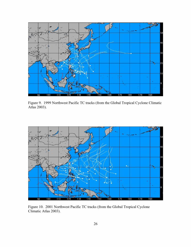
Figure 9. 1999 Northwest Pacific TC tracks (from the Global Tropical Cyclone Climatic Atlas 2003).
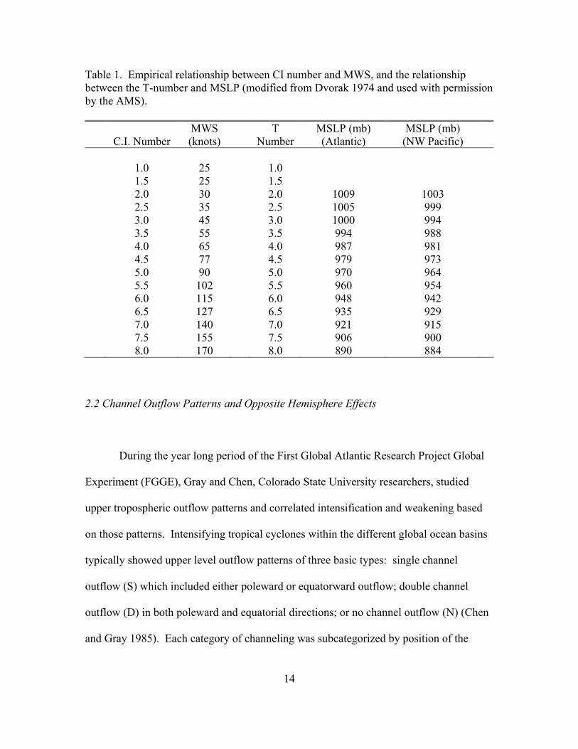
Figure 10. 2001 Northwest Pacific TC tracks (from the Global Tropical Cyclone Climatic Atlas 2003).

27
Figures 8 through 10 depict the tracks of northwestern Pacific Ocean tropical cyclones
during 1997, 1999, and 2001. Based on the tightest grouping of tracks, it is easy to
conclude that the majority of storms during the past several years fall under DeMaria’s
criteria of low latitude. Therefore, it is expected that given similar climatological
conditions, future tropical cyclones will be sensitive to the effects of vertical shear. In
addition, typhoons located north of about 30°N will be caught up in the mid-latitude
westerlies, therefore becoming extratropical and weaken rapidly due to high shear.
For tropical cyclones located between 20°N and 29°N, DeMaria does not make
specific reference as to the effects of vertical shear. Therefore, it is possible that the
effects cannot be treated individually, but rather as a secondary or tertiary mechanism
supporting an overall intensification or dissipation trend.
2.5.3 Air-Sea Interactions. The interactions between air and sea closely parallel the sea
surface temperature discussion in Section 2.5.1. The main focus is the process by which
the typhoon extracts energy from the boundary layer near the ocean surface. This is
accomplished through high percentages of relative humidity (RH). RH unlocks a key to
the development of the MPI through deep convection in the eyewall. As latent heat
release occurs, larger percentages of RH provide needed water vapor, and Cb towers
grow higher into the troposphere, enhancing the overall strength of the TC.
Holland (1997) found that a “derived MPI is highly sensitive to the surface RH
under the eyewall, to the height of the warm core, and to transient changes of SST.” The
limitations on how high the eyewall can develop stem from the availability of moist
entropy between the ocean surface and the base of the clouds. Here, Holland defines

28
moist entropy as equivalent potential temperature, θE, which is a function of pressure and
temperature. As the tropical cyclone’s central pressure lowers during constant or
relatively constant SST, θE increases. This process develops a positive feedback
mechanism which in turn lowers the surface pressure. Therefore, as long as the central
pressure is able to decrease, the TC should intensify. However, there is a limitation to the
amount of energy the storm can extract, which is primarily based on overall movement.
Storms which stagnate can undergo weakening even while they continually feed off of
the ocean water vapor via evaporation and latent heat release.
Evaporation of water vapor from the ocean surface is a cooling process and will
begin to lower the SST over time. This effect is not as drastic as upwelling, but it has
been shown that tropical cyclones which move across waters previously occupied by a
system do not have access to the same degree of surface temperature (i.e., moist entropy).
The wake of a tropical cyclone leaves cooler surface waters, and consequently can
decrease the amount of intensification of a subsequent TC via cooler inflow (see also
Black and Shay 1998). In a similar study, Sikora et al. (1976) found that “measuring
700 mb θE is a useful way to measure the total thermodynamic energy because it
accounts for both latent and sensible heat. Their study parallels the work done by
Holland (1997) by correlating minimum central surface pressure to 700 mb θE.”
2.6 Upper Tropospheric Flow Transitions
Upper tropospheric flow transitions (UTFT) provide an alternate means of
intensification by enabling tropical cyclones to intensify without explicitly relying upon a

29
change of conditions at the surface. In particular, UTFT usually change the
environmental winds which make access to outflow channels more conducive. This
process is accomplished via relaxation of a major upper-level trough west of the tropical
cyclone as anticyclogenesis occurs near the equatorward edge of the trough (Davidson
and Kar 2002). As relaxation occurs, large-scale vertical shear is also reduced, allowing
for more vigorous convection to develop within the eyewall. A “new” trough develops
downstream of the TC and opens up access to the midlatitude westerlies and tropical
easterlies. This outflow provides even further intensification by increasing the ventilation
of heat and mass from the cyclone core. However, if the typhoon eye begins to migrate
into the westerlies, increased shear will induce weakening.
Davidson and Kar (2002) as well as Chen and Gray (1985) found that rapid
intensification may occur once access to these upper level outflow channels has been
established. In addition, upper level cyclonic circulation is enhanced, which leads to the
onset of more moist, deep convection. Sadler (1978) also showed that intensification was
favorable as the tropical cyclone moved into optimum proximity with the UC. This
rationale is also consistent with the PV superposition and anomalies suggested by
Molinari et al. (1998). Even though UTFT cannot be treated individually, as a
mechanism for TC intensification, they play an integral part of the overall dynamics.
Coupled with outflow channel access and PV superposition, UTFT provide useful insight
into the synoptic patterns at 200 mb which can lead to explosive intensification.
Understanding upper tropospheric flow transitions, as well as TUTT interactions and
channel outflow patterns, provide better awareness in forecasting tropical cyclone
intensity changes.

30
III. Methodology
3.1 Introduction
The overall goal of this research is to data mine atmospheric parameters
responsible for typhoon rapid intensification and weakening and to validate the
usefulness of using these parameters in the forecast process. These predictors vary from
environmental conditions (such as sea surface temperature) to model derived fields (such
as wind shear). Currently, JTWC only uses the Dvorak Technique to forecast
intensification trends, and the objective of this research is to broaden the tools used in
these forecasts. In order to meet this expectation, CART data mining is used to develop
the new tools. This analysis employs various splitting rules (discussed further in Section
3.3.1), combined with both simple linear regression and classification analysis
techniques.
3.2 Data Acquisition
3.2.1 Storm Selection. As mentioned in Section 1.2, using typhoons from different
climatological regimes (EN, LN, NU) is important. These regimes serve as yet another
predictor in supporting or inhibiting rapid intensification. Of the total number of tropical
events in 1997, 1999, and 2001, 27 storms are selected for research since specific criteria
needed to be met. These 27 storms are all typhoon strength or greater and exhibit some
form of rapid intensification or rapid weakening during their lifecycle. The criteria for
31
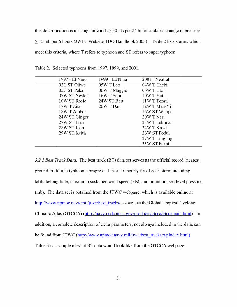
this determination is a change in winds > 50 kts per 24 hours and/or a change in pressure
> 15 mb per 6 hours (JWTC Website TDO Handbook 2003). Table 2 lists storms which
meet this criteria, where T refers to typhoon and ST refers to super typhoon.
Table 2. Selected typhoons from 1997, 1999, and 2001.
1997 - El Nino 1999 - La Nina 2001 - Neutral 02C ST Oliwa 05W T Leo 04W T Chebi 05C ST Paka 06W T Maggie 06W T Utor 07W ST Nestor 16W T Sam 10W T Yutu 10W ST Rosie 24W ST Bart 11W T Toraji 17W T Zita 26W T Dan 12W T Man-Yi 18W T Amber 16W ST Wutip 24W ST Ginger 20W T Nari 27W ST Ivan 23W T Lekima 28W ST Joan 24W T Krosa 29W ST Keith 26W ST Podul 27W T Lingling 33W ST Faxai
3.2.2 Best Track Data. The best track (BT) data set serves as the official record (nearest
ground truth) of a typhoon’s progress. It is a six-hourly fix of each storm including
latitude/longitude, maximum sustained wind speed (kts), and minimum sea level pressure
(mb). The data set is obtained from the JTWC webpage, which is available online at
http://www.npmoc.navy.mil/jtwc/best_tracks/, as well as the Global Tropical Cyclone
Climatic Atlas (GTCCA) (http://navy.ncdc.noaa.gov/products/gtcca/gtccamain.html). In
addition, a complete description of extra parameters, not always included in the data, can
be found from JTWC (http://www.npmoc.navy.mil/jtwc/best_tracks/wpindex.html).
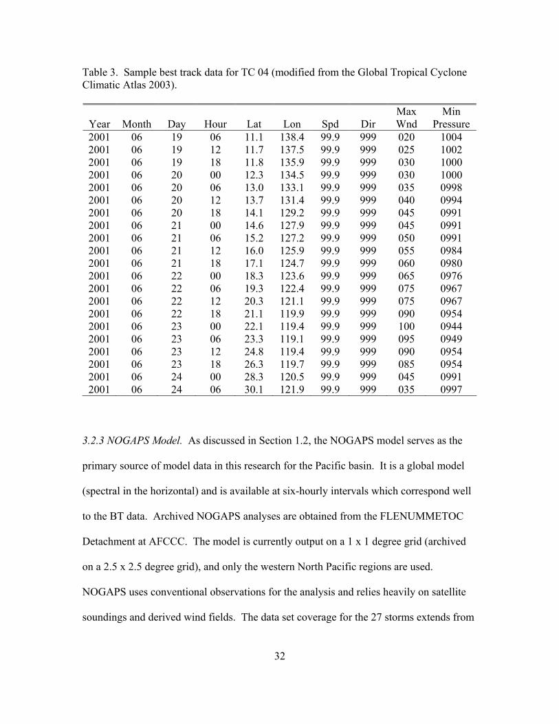
Table 3 is a sample of what BT data would look like from the GTCCA webpage.
32
Table 3. Sample best track data for TC 04 (modified from the Global Tropical Cyclone Climatic Atlas 2003).
Year
Month
Day
Hour
Lat
Lon
Spd
Dir
Max Wnd
Min Pressure
2001 06 19 06 11.1 138.4 99.9 999 020 1004 2001 06 19 12 11.7 137.5 99.9 999 025 1002 2001 06 19 18 11.8 135.9 99.9 999 030 1000 2001 06 20 00 12.3 134.5 99.9 999 030 1000 2001 06 20 06 13.0 133.1 99.9 999 035 0998 2001 06 20 12 13.7 131.4 99.9 999 040 0994 2001 06 20 18 14.1 129.2 99.9 999 045 0991 2001 06 21 00 14.6 127.9 99.9 999 045 0991 2001 06 21 06 15.2 127.2 99.9 999 050 0991 2001 06 21 12 16.0 125.9 99.9 999 055 0984 2001 06 21 18 17.1 124.7 99.9 999 060 0980 2001 06 22 00 18.3 123.6 99.9 999 065 0976 2001 06 22 06 19.3 122.4 99.9 999 075 0967 2001 06 22 12 20.3 121.1 99.9 999 075 0967 2001 06 22 18 21.1 119.9 99.9 999 090 0954 2001 06 23 00 22.1 119.4 99.9 999 100 0944 2001 06 23 06 23.3 119.1 99.9 999 095 0949 2001 06 23 12 24.8 119.4 99.9 999 090 0954 2001 06 23 18 26.3 119.7 99.9 999 085 0954 2001 06 24 00 28.3 120.5 99.9 999 045 0991 2001 06 24 06 30.1 121.9 99.9 999 035 0997
3.2.3 NOGAPS Model. As discussed in Section 1.2, the NOGAPS model serves as the
primary source of model data in this research for the Pacific basin. It is a global model
(spectral in the horizontal) and is available at six-hourly intervals which correspond well
to the BT data. Archived NOGAPS analyses are obtained from the FLENUMMETOC
Detachment at AFCCC. The model is currently output on a 1 x 1 degree grid (archived
on a 2.5 x 2.5 degree grid), and only the western North Pacific regions are used.
NOGAPS uses conventional observations for the analysis and relies heavily on satellite
soundings and derived wind fields. The data set coverage for the 27 storms extends from

33
5°N to 47.5°N latitude and from 165°W to 100°E longitude. One initial and very
important consideration in using this model data with ~ 150 nm between grid points, is to
most closely match the typhoon center to the nearest latitude and longitude of the model
domain. In order to accomplish this task, a MATLAB program is written to associate the
typhoon to the nearest grid point. This technique assumes a certain margin of error since
the maximum distance could be as large as 106 nm if the core is exactly between grid
points. However, since no other available model provides the needed coverage, this
potential error is noted during the collection of the model fields. Table 4 lists the
different model fields used in this research
Table 4. NOGAPS model fields. Level Model Fields Surface T, RH, U, V 1000 mb T, RH, U, V 850 mb T, RH, U, V 200 mb T, U, V
where T is temperature, RH is relative humidity, U is the east-west wind component, and
V is the north-south wind component. In addition to the normally computed fields
provided by AFCCC, another MATLAB program is created to calculate surface-200 mb,
1000-200 mb, and 850-200 mb wind speed and directional shear as well as surface,
1000 mb, 850 mb, and 200 mb winds. A complete listing of both MATLAB programs is
found in Appendices A and B.
It is also important to note that some of the model data are unavailable during
brief periods within the lifecycle of six typhoons. The storms which have missing data
are listed in Table 5.

34
Table 5. Storms with missing model fields.
1997 2001 Paka (05C) Chebi (04W) Nestor (07W) Man-Yi (12W) Wutip (16W) Nari (20W)
Although these storms are missing some data, they are still included in the overall
analysis. By contrast, all of the selected storms in 1999 have a complete archive of the
model fields.
3.2.4 Sea Surface Temperatures. Since the primary source of heat and energy required to
sustain typhoon development is the ocean surface, SST data over the entire lifecycle of
each typhoon are incorporated to the overall database. SSTs are also obtained from the
FLENUMMETOC Detachment at AFCCC. These data are derived from the Air Force
Weather Agency (AFWA) Surface Temperature (SFCTMP) Model. An in-depth
discussion on the SFCTMP model is found in Kopp (1995), however the process is
briefly discussed below.
For all water points in the SFCTMP Model, unchanged US Navy SST analyses
are used. These analyses are received once daily, and each analysis is a global snapshot
valid at 1200 Coordinated Universal Time (UTC). The US Navy collects SST values
(from surface observations and satellite algorithms) which are mapped on a 0.25 x 0.25
degree grid, however the SFCTMP Model operates on a 0.125 x 0.125 degree grid. In
order to populate the SFCTMP domain, a bilinear interpolation is used to remap the SST
values to the proper grid spacing. In addition, the SST data are quality checked during

35
each model cycle. If any location over water has a temperature colder than 270 K or
warmer than 310 K, that value is discarded, and the value from the previous cycle is used.
“This procedure not only prevents unrealistic SSTs, but avoids an excessively noisy
analysis” (Kopp 1995).
3.2.5 CPC Teleconnection Indices. The two teleconnection indices used in this research
are the Southern Oscillation Index (SOI) and the Multivariate ENSO Index (MEI). The
teleconnection indices are used to draw a relationship to EN, LN, and NU years. Both of
these indices are obtained from the Climate Prediction Center (CPC) website
(http://www.cdc.noaa.gov/ClimateIndices/) under the Niño 4 grid box, which is located
between 5°N and 5°S latitude and between 150°W to 160°E longitude. A description of
the standardized SOI can be found in Randall (2002). In essence, the SOI is the
difference in the standardized anomalies of sea level pressure between Darwin, Australia
and the Pacific Island of Tahiti (D’Aleo and Grube 2002, Ford 2000). Generally, a
positive value of SOI is associated with EN phases, and a negative value is associated
with LN phases. In addition to the SOI, a newly developed multivariate index is also
used.
The MEI was developed to provide a new comprehensive data set that
incorporates multiple factors, including air temperatures, sea surface temperatures, sea
level pressure, surface wind, and cloudiness (D’Aleo and Grube 2002). Although the
MEI does not provide coverage on a monthly basis, as the SOI does, it was developed in
anticipation of becoming a new standard for measuring climatic changes. The MEI is
measured on a bi-monthly basis (where the January value is the December-January

36
timeframe and the value is centered between the two months). D’Aleo and Grube (2002)
suggest that significant ENs have MEIs > 1 while significant LNs have MEIs < -1.
Values of MEI between -1 and 1 are assumed to incorporate NU regimes, although the
literature did not make specific reference to these values. CPC also maintains other
various teleconnection indices, however the SOI and MEI are the only two deemed useful
in this research. It is significant to note that there is some inherent error in using the
Niño 4 grid box due to its location in the Pacific Ocean.
The majority of the typhoons originate near the international date line, however
they propagate well past the western most edge of the grid box (which remains stationary
regardless of the climatic regime). Therefore, some of the lifecycle is not covered by the
index. In addition, due to the Coriolis force, tropical cyclones are not usually observed
within 5 degrees north or south latitude of the equator. Thus, none of the storms are
located under the northern most edge of the Niño 4 grid box. However, given the
availability of climatic information and the association to tropical cyclones, SOI and MEI
values are assumed to be representative of the entire lifecycle of the storm.
3.3 CART Overview
Classification and regression tree analysis was developed in the early 1980s and
has become one of the primary drivers in data mining research. The overall objective is
to use decision trees in mapping a target variable (dependent response) from a set of
predictors (independent variables). Classification and regression analyses both use
decision trees, however only the classification analysis is considered important to this

37
research. This scheme utilizes a binary, recursive partitioning, tree growing algorithm
which was developed by Breiman et al. (1984).
The classification approach uses a non-parametric statistical analysis which
begins with the parent node. The data are divided into one of two child nodes according
to a “yes” response (i.e., meets the splitting rule condition, discussed further in Section
3.3.1.1) or a “no” response (i.e., does not meet the splitting rule condition). Benz (2003)
provides a detailed example of meeting splitting rule conditions. In order for the parent
node to be split into two purer child nodes where purer refers to improved homogeneity
of the data, the target variable must be categorical (e.g., A, B, C or 1, 2, 3). If the target
variable contains discrete data, it is necessary to define these data as categorical variables
(or “dummy” variables). The remaining predictors can also be defined categorically or
retain their original values. Once the target variable has the correct format, the decision
tree building process begins.
CART continues to split each subsequent child node until the optimal terminal
node is reached, and it considers all possible splits for each of the predictors in the data
set. The total number of splits is determined by the product of the predictors and number
of records in the data set. For example, if there are 10 different predictors and 100
records of data, CART will consider 1000 different splits in formulating the optimal tree.
A complete treatment of terminal node calculation is found in Breiman et al. (1984).
After the full tree is grown, CART displays the optimal tree, showing the best splits
based on the target variable. If it is undesirable to define the target variable categorically,
then the regression method needs to be employed.

38
The CART regression scheme does not require a categorical target variable,
however the only splitting rule used is least squares (discussed further in Section 3.4).
Similar to the classification scheme, a regression analysis also creates a decision tree
from which inferences about the partitioned data may be made.
3.3.1 Methods
3.3.1.1 Tree Splitting Methods. In the classification analysis, there are six different
splitting functions. Only two, Gini and Twoing, are employed for this research due to
time constraints. The Gini function seeks to isolate the largest subset of data from the
remaining population such that the largest group is placed in one child node and the rest
in the other child node. For example, consider a data set with the following classified
population (and quantity listed in parentheses): A (40), B (30), C (20), D (10). The Gini
function would review the population of 100 and distribute Class A into one child node
while Classes B, C, and D would go to the other child node. Then, at the second splitting
level in the tree, Gini would distribute Class B into one child node, leaving Classes C and
D in the other node. Finally, the third splitting level would result in one terminal node
containing Class C and the remaining terminal node containing Class D. In total, there
would be four terminal nodes, each with the highest level of homogeneity (see Figure 11
for a graphical look at this process).
The Twoing function operates in a similar fashion, however it attempts to isolate
the same quantity of data among the child nodes. In Figure 12, notice that since the total
sample space between Classes A and D (50) is the same as Classes B and C (50), Twoing
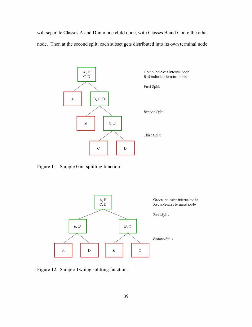
39
will separate Classes A and D into one child node, with Classes B and C into the other
node. Then at the second split, each subset gets distributed into its own terminal node.
Figure 11. Sample Gini splitting function.
Figure 12. Sample Twoing splitting function.

40
If the population does not consist of perfect splits (i.e., 50-50), as illustrated in this
example, the Twoing function will attempt to make the best split where 1/2 of the data is
in each child node. In order to understand each splitting function, a brief description is
given below.
The mathematical expression for the Gini function is given by
( ) ( )| |j i
p i t p j t≠∑ (6)
where ( )|p i t is the probability of an object selected at random being distributed into
Class i given Class t; and ( )|p j t is the probability of an object selected at random being
distributed into Class j given Class t. In Gini, “the impurity (or lack of homogeneity) is
calculated by subtracting the sum of squared probabilities of each class within the given
node summed over all levels of the categorical variable” (Steinberg and Colla 1995).
This function is best thought of as peeling the layers (of an onion, for example) in order
to isolate each subclass.
The mathematical expression for the Twoing function is given by
( ) ( )2
| |4
L RL R
j
p p p j t p j t
− ∑ (7)
where ( )| Lp j t is the probability of an object being distributed into Class j given a left
terminal node, and ( )| Rp j t is the probability of an object being distributed into Class j
given a right terminal node (Breiman et al. 1984). In Twoing, “the objective is to make
the likelihood that a given class goes to the left as different as possible from the
probability that it goes to the right” (Benz 2003). Furthermore, Equation 7 is maximized

41
when Lp and Rp each equal 0.5. Both splitting functions result in the same four terminal
nodes (each containing an individual sample space), however the process in deriving the
terminal nodes varies slightly. Breiman et al. (1984) did note that twoing the data gives
“strategic” splits and informs the user of class similarities. Twoing is accomplished by
grouping together large numbers of classes which have similar characteristics.
3.3.1.2 Pruning. The tree will continue to grow (splitting child nodes) until it is no
longer able to split or until a pre-defined node size is reached. At this terminal node
junction, the tree is at its largest size. There may, however, be nodes which can be
removed (pruned) to improve the overall effectiveness of interpreting the outcome. For
example, CART will remove nodes when each child has the same classification (such as
Class A). This pruning is meaningful because the overall purpose is to achieve node
purity by “complete” homogeneity within the node. Having two child nodes with the
same class assignment does not provide more information than examining the parent
node. In addition, CART will prune where the gain in improvement score (see Section
3.3.1.4) exceeds the loss in homogeneity. Breiman et al. (1984) suggest letting the tree
grow to a maximum (i.e., splitting until the terminal nodes contain the smallest allowable
node size), however this outcome may result in hundreds of terminal nodes. In this way,
the interpretation becomes impractical, and the nodes need to be collected back toward
the parent node. This process is called upward pruning, and CART will display each
phase of the splitting process (allowing the user to manually upward prune at each level
to examine the effects).

42
3.3.1.3 Cross Validation. If the data set is large enough (i.e., thousands of records), the
user can divide the data into a learn sample and a test sample for validation of the final
tree. However, in this research, the data set is too small to employ the learn and test
sample procedure, therefore a 10-fold cross validation technique is used. According to
Steinberg and Colla (1995), “the core idea of cross validation is that each observation is
included in both the test sample and the learning sample.” The tree is grown for the first
time using all of the data in order to provide an error rate reference. In 10-fold cross
validation, the data are divided into approximately 10 equal and random subsets, and the
process of growing the trees is repeated 10 separate times from the beginning. In each
stage of cross-validation, nine subsets of the data are used to build the model (learn data),
and one subset is used for testing. For each stage of testing, a different subset of the data
is used whereas the same subset is not used twice. Also, the error rates are computed for
each tree during that step in the sequence. When the 10 cycles are complete, the error
rates from all 10 samples are summed in order to provide the overall error of the tree.
This method is appealing because once an observation is used for building the
model, it is not available for testing and thus it does not influence the growth of the tree
during that stage. Also, since every observation is used exactly once while the tree is
being built, it has an equal probability of being correctly or incorrectly classified.
Therefore, the total misclassification rates are correct for the complete data set (Steinberg
and Colla 1995). Figure 13 shows a graphical look at the 10-fold cross validation
process.

43
Figure 13. Graphical depiction of 10-fold cross validation (modified from Salford Systems 1995).
3.3.1.4 Improvement Scores. As each parent node splits, the assumption is that each child
node has less impurity (i.e., more homogeneity in the data) than the parent. In building
the optimal tree, CART measures the decrease in impurity from node to node, and this
overall value is called the improvement score. Breiman et al. (1984) state that the
improvement score is calculated by subtracting the sums of the child node impurities,
multiplied by each respective probability of a left or right node distribution, from the
parent node impurity. Figure 14 shows a graphical depiction of the split and resulting
impurities. The equation of the improvement score after the split is given by
( ) ( )( )P L L R Rscore I I prob I prob= − + (8)
where score is the improvement score, IP is the parent node impurity, IL is the left child
node impurity, probL is the probability of distributing to the left child node, IR is the right
child node impurity, and probR is the probability of distributing to the right child node.

44
Figure 14. Example of an improvement score.
The improvement score in this example is 40 600.8 0.4 0.6 0.28100 100
− + = . Each
time there is a split, an improvement score is calculated, and this score measures how
well the split improves the predictive performance of the tree.
3.3.1.5 Class Assignments. One of the most important elements in assessing the overall
quality of the classification tree is the percent error misclassification. The percent error
misclassification stems directly from the class assignment in each terminal node, which is
computed with Bayes’ Theorem (Montgomery and Runger 2002). Equation 9 is used to
determine the probability of a record going into a left child node (L), given it is of Class n
( ) ( ) ( )( ) ( ) ( ) ( ) ( ) ( )
0 00
0 0 1 1 2 2
||
| | |p L n p n
p n Lp L n p n p L n p n p L n p n
=+ +
(9)
where nx is Classes 0, 1, and 2. The individual probabilities, ( )| xp L n and ( )xp n , can
be determined by two different means. When Priors Data is used, the probability of Class
n is computed as the number of records in Class n divided by the sum of records (across

45
all classes) in that node. Priors Data states that the probability of each class is equal to
the distribution of the class in the sample. When Priors Equal is used, the probability of
Class n is exactly the inverse of the number of classes. Priors Equal states that the
probability of each class is equal, regardless of the frequency distribution. The following
example illustrates Priors Equal probability where the distribution of cases is
Parent Left Right Class 0 1037 241 796 Class 1 74 50 24 Class 2 87 3 84
The within-node probabilities are calculated as
Left Right Class 0 0.247 0.373 Class 1 0.717 0.158 Class 2 0.036 0.469
where the class assignment for the left node is Class 1, and the class assignment for the
right node is Class 2. Thus, all of the records not of Class 1 (left node) and Class 2 (right
node) are misclassified. The percent error misclassification is based on the summation of
the misclassifications per class in each terminal node of the entire tree.
3.3.2 Research Predictors. In order to employ the data mining software, 41 different
predictors are selected, ranging from continuous numerical values to categorical values.
Table 6 shows a list of the predictors used in this research. It is important to note that the
predictors in italics are defined categorically according to discussions in Chapter 2. The
rules which govern the categories are shown in Table 7, and the values are listed in Table
8. CLIMO is also categorical to account for the climatic regime once the data is merged.
However, it’s not included in Tables 7 and 8 because of a lack of favorable and
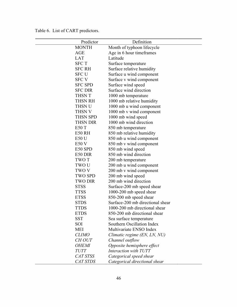
46
Table 6. List of CART predictors.
Predictor Definition MONTH Month of typhoon lifecycle AGE Age in 6 hour timeframes LAT Latitude SFC T Surface temperature SFC RH Surface relative humidity SFC U Surface u wind component SFC V Surface v wind component SFC SPD Surface wind speed SFC DIR Surface wind direction THSN T 1000 mb temperature THSN RH 1000 mb relative humidity THSN U 1000 mb u wind component THSN V 1000 mb v wind component THSN SPD 1000 mb wind speed THSN DIR 1000 mb wind direction E50 T 850 mb temperature E50 RH 850 mb relative humidity E50 U 850 mb u wind component E50 V 850 mb v wind component E50 SPD 850 mb wind speed E50 DIR 850 mb wind direction TWO T 200 mb temperature TWO U 200 mb u wind component TWO V 200 mb v wind component TWO SPD 200 mb wind speed TWO DIR 200 mb wind direction STSS Surface-200 mb speed shear TTSS 1000-200 mb speed shear ETSS 850-200 mb speed shear STDS Surface-200 mb directional shear TTDS 1000-200 mb directional shear ETDS 850-200 mb directional shear SST Sea surface temperature SOI Southern Oscillation Index MEI Multivariate ENSO Index CLIMO Climatic regime (EN, LN, NU) CH OUT Channel outflow OHEMI Opposite hemisphere effect TUTT Interaction with TUTT CAT STSS Categorical speed shear CAT STDS Categorical directional shear
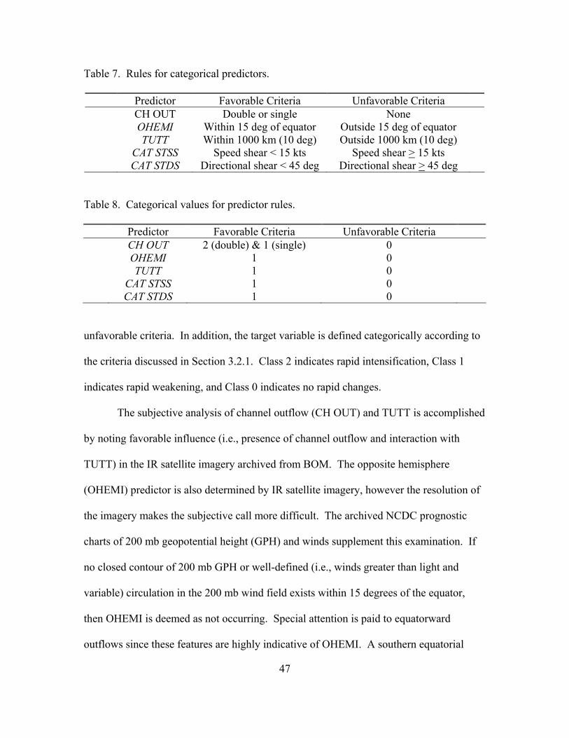
47
Table 7. Rules for categorical predictors.
Predictor Favorable Criteria Unfavorable Criteria CH OUT Double or single None OHEMI Within 15 deg of equator Outside 15 deg of equator TUTT Within 1000 km (10 deg) Outside 1000 km (10 deg) CAT STSS Speed shear < 15 kts Speed shear > 15 kts CAT STDS Directional shear < 45 deg Directional shear > 45 deg
Table 8. Categorical values for predictor rules. Predictor Favorable Criteria Unfavorable Criteria CH OUT 2 (double) & 1 (single) 0 OHEMI 1 0 TUTT 1 0 CAT STSS 1 0 CAT STDS 1 0
unfavorable criteria. In addition, the target variable is defined categorically according to
the criteria discussed in Section 3.2.1. Class 2 indicates rapid intensification, Class 1
indicates rapid weakening, and Class 0 indicates no rapid changes.
The subjective analysis of channel outflow (CH OUT) and TUTT is accomplished
by noting favorable influence (i.e., presence of channel outflow and interaction with
TUTT) in the IR satellite imagery archived from BOM. The opposite hemisphere
(OHEMI) predictor is also determined by IR satellite imagery, however the resolution of
the imagery makes the subjective call more difficult. The archived NCDC prognostic
charts of 200 mb geopotential height (GPH) and winds supplement this examination. If
no closed contour of 200 mb GPH or well-defined (i.e., winds greater than light and
variable) circulation in the 200 mb wind field exists within 15 degrees of the equator,
then OHEMI is deemed as not occurring. Special attention is paid to equatorward
outflows since these features are highly indicative of OHEMI. A southern equatorial

48
ridge is observed to help enhance the equatorward outflow. In addition, it appears that
OHEMI effects were more influential to western Pacific events than events in the central
Pacific. This observation might certainly be a factor when considering climatic regimes
because EN years tend to show typhoon development further east and south whereas LN
years tend to show typhoon development further west.
Initial rapid intensification almost always occurs when CH OUT is established 6
to 12 hours earlier. The dissipation of CH OUT (change in predictor category) is not
specifically addressed in the literature, therefore it is assumed no longer occurring when a
typhoon loses the majority of its characteristics (eye and symmetry) and/or is sheared by
mid-latitude westerly flow. For storms which follow an extratropical path, mid-latitude
flow usually affects the last 24 to 36 hours of their lifecycle.
The TUTT, which is a transient feature, is reserved exclusively for influences by
the 200 mb trough in the central Pacific, although there are some instances of interactions
with major shortwave troughs over eastern Asia and the western Pacific. These
interactions are usually picked up by channel outflows, therefore they are not counted
twice. If these trough effects don’t have channel outflows occurring at the same time,
they are not counted at all in the analysis. It is also noted that there are no TUTT
influences during LN events. This lack of occurrence is most likely due to the fact that
typhoons originate too far west in the Pacific, and they remain outside of an optimal
north-northwest interlocking position to the upper trough during the course of their
lifecycle.
Even though some of the predictors, such as STSS, STDS, and SST already have
predefined intensification or weakening criteria, they are still included in the analyses. In

49
addition, categorical values of STSS and STDS are included to examine any differences
from the actual values of speed and directional shear. These variables are included to
validate the current rules-of-thumb and to see if JTWC guidelines change based on the
three year data set. The predictors without predefined rules-of-thumb are data mined to
determine relationships, if any, with the target variable. Predictors which are found
conducive to typhoon rapid intensification or rapid weakening thus become the focus for
deeper CART analyses and are discussed further in later chapters.
3.4 Statistical Overview
3.4.1 Introduction. Regression analysis is used to explore the relationships between two
or more variables. This examination is accomplished with simple linear regression (one
predictor, an independent variable such as X and one response, a dependent variable such
as Y) or multiple linear regression (several predictors such as 1 2, , nX X X… and one
response such as Y). There are several different avenues of regression that can be
explored, ranging from hypothesis testing to model adequacy. Each of these methods
involves the properties of the least squares estimators, which is the same procedure
CART employs in a regression analysis. Since the target variable in this research is
categorical, the classification analysis is used. However, regression analysis is used to
validate the accuracy of the NOGAPS model (see Chapter 4).

50
3.4.2 Simple Linear Regression. The method of least squares approximates a line
connecting points ( ) ( ) ( )1 1 2 2, , , ,n nX Y X Y X Y… which has the equation
0ˆ
i i iY xβ β ε= + + (10)
where Y is an approximation of the true Y, 0 , iβ β are coefficients of regression, and iε
is a margin of error. The intercept, 0β , and slope, 1β , are defined as
1ˆ ˆ
o y xβ β= − (11)
1 1
11 2
2 1
1
ˆ
n n
i ini i
i ii
n
ini
ii
y xy x
n
xx
n
β
= =
=
=
=
−
= −
∑ ∑∑
∑∑
(12)
where 1
1 n
ii
y yn =
= ∑ and 1
1 n
ii
x xn =
= ∑ (Montgomery and Runger 2002). These equations
can therefore be extended to include j predictors in the domain of X (for multiple linear
regression analyses). A scatter plot of data which yields a strong correlation between Y
and iX would have minimal errors, ie , or residuals defined as
ˆi i ie y y= − (13)
since this is the difference between the estimated (regression) value of y and the true
value of y. Using regression analysis requires the following assumptions discussed by
Montgomery and Runger (2002). These assumptions allow the user to make inferences
based on the regression, and the overall model capability is often noted by the 2R
coefficient.

51
1) Estimation of the model parameters requires assumption that errors are uncorrelated random variables with mean zero and constant variance. 2) Tests of hypothesis and interval estimation require the errors be normally distributed. 3) The order of the model is correct, which assumes the phenomenon actually behaves in a linear or first-order manner. The adequacy of the model can also be judged by the coefficient of determination
2R . Since there is no perfect model, 2R values rarely reach unity and higher values
indicate better effectiveness. “Qualitatively, the 2R can be interpreted as the proportion
of the variation of the predictand (proportional to TSS ) that is “described” or “accounted
for” by the regression ( RSS )” (Wilks 1995). In multiple linear regression, adding more
predictors inherently increases 2R , and it can be difficult to determine whether the
increase is providing useful information about the new predictor. Therefore 2adjR is used
to compensate for the number of parameters in a regression model. The equations for 2R
and 2adjR are shown in Equations 14 and 15
2 1R E
T T
SS SSRSS SS
= = − (14)
( )
( )
2 1
1
E
adjT
SSn p
R SSn
−= −
−
(15)
where RSS is the regression sum of squares, TSS is the total sum of squares, ESS is the
error sum of squares, and ( )n p− and ( )1n − are degrees of freedom (Montgomery and
Runger 2002).

52
Another common measure of accuracy that can be used is the mean-squared error
(MSE). The MSE averages the individual squared differences between the gridded
forecast and observed fields at each of the M grid points. This is defined mathematically
in Equation 16.
( )2
1
1 M
m mm
MSE y oM =
= −∑ (16)
“Often the MSE is expressed as its square root, the root-mean squared error (RMSE).
RMSE MSE= (17)
This form of expression has the advantage that it retains the units of the forecast variable
and is thus more easily interpretable as a typical error magnitude” (Wilks 1995).

53
IV. Analysis and Results
4.1 Introduction
This chapter discusses the performance of the selected predictors from Chapter 3
and the results of the CART classification analyses. Initially, a simple linear regression
study is done on the NOGAPS wind analyses to determine accuracy when compared to
the BT data (i.e., nearest ground truth). This regression study determines how well the
model depicts the changes in the environment that lead to rapid changes in typhoon
intensity. In addition, a comparison could be done with MSLP and NOGAPS pressure
analyses, however since pressure is not available in the BT data archive for the majority
of this research, this study is not performed. The BT data archive starting with 2001 can
be used in an MSLP regression assessment.
4.2 Regression Analysis of NOGAPS and Best Track Data
It is important to establish confidence in the NOGAPS model early in the
research, since it is the primary source of data. In general, model data are never used in
determining BT data. NOGAPS is only used in cases where the standard techniques of
determining maximum wind speed (Dvorak CI relationship, synoptic or microwave
patterns) are not well fit to the storm, such as when typhoons are not well developed or as
in a midget typhoon (Vilpors personal correspondence 2003). A description of midget
typhoons can be found in the TC Forecasters’ Reference Guide, NRL Website (1998).

54
The NOGAPS model employs a multivariate optimum interpolation analysis to
include, but not limited to, radiosonde, aircraft, and satellite measurements. In addition,
it should be noted that the analyses of TC are almost too large in horizontal extent due to
the global model resolution (UCAR website 2004). Furthermore, since 1990, the data
have been “bogused” to account for the position and intensity of a typhoon. Goerss and
Jeffries (1994) provide further information as to the nature of bogusing the model.
In order to perform the initial regression analysis, the SAS Institute statistical
software package JMP is used to determine RMSE and correlation strength between the
NOGAPS wind analyses and the BT data. Table 9, sorted by typhoon name, shows a
breakdown of these statistics, where a fit line technique is used in calculating RMSE.
The RMSE values can also be calculated in a similar fashion by using a fit model analysis
with standard least squares.
This initial analysis shows a fairly high correlation strength, however the
regression fit line between NOGAPS and BT accounts for only 1/3 of the variance of the
model. In fact, scatter plots of the BT data against time show more of an exponential rise
whereas the NOGAPS data indicate a multi-ordered polynomial fit. It is probable that if
a cubic, quadratic, or higher ordered fit is attempted, the RMSE values would decrease
(i.e., for a better linear fit, there should be less variability in the data points). On average,
the RMSE values indicate 24.849 kts variation between NOGAPS and BT data.
Although the model handles the trends in the wind speeds well, there is an error of about
25 kts. However, given that a linear fit (and not higher ordered fit) is used, the NOGAPS
model can be employed with a reasonable level of confidence that it is accurately
depicting the typhoon surface wind strength.
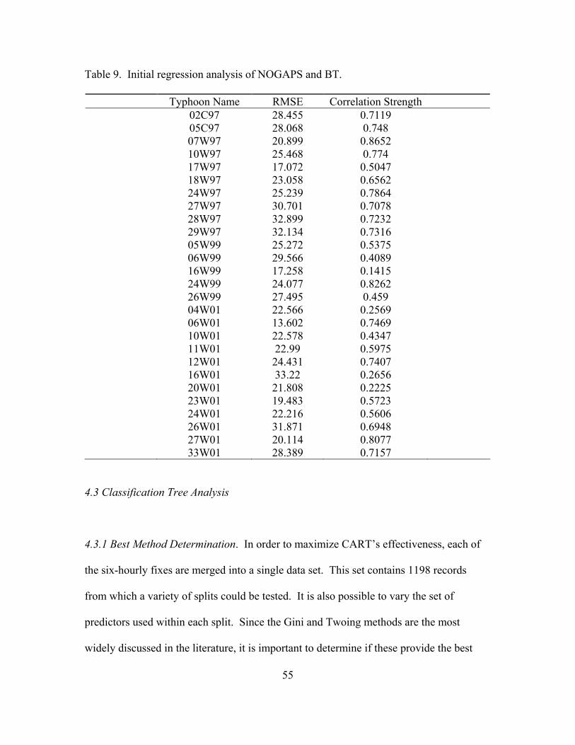
55
Table 9. Initial regression analysis of NOGAPS and BT.
Typhoon Name RMSE Correlation Strength 02C97 28.455 0.7119 05C97 28.068 0.748 07W97 20.899 0.8652 10W97 25.468 0.774 17W97 17.072 0.5047 18W97 23.058 0.6562 24W97 25.239 0.7864 27W97 30.701 0.7078 28W97 32.899 0.7232 29W97 32.134 0.7316 05W99 25.272 0.5375 06W99 29.566 0.4089 16W99 17.258 0.1415 24W99 24.077 0.8262 26W99 27.495 0.459 04W01 22.566 0.2569 06W01 13.602 0.7469 10W01 22.578 0.4347 11W01 22.99 0.5975 12W01 24.431 0.7407 16W01 33.22 0.2656 20W01 21.808 0.2225 23W01 19.483 0.5723 24W01 22.216 0.5606 26W01 31.871 0.6948 27W01 20.114 0.8077 33W01 28.389 0.7157
4.3 Classification Tree Analysis
4.3.1 Best Method Determination. In order to maximize CART’s effectiveness, each of
the six-hourly fixes are merged into a single data set. This set contains 1198 records
from which a variety of splits could be tested. It is also possible to vary the set of
predictors used within each split. Since the Gini and Twoing methods are the most
widely discussed in the literature, it is important to determine if these provide the best
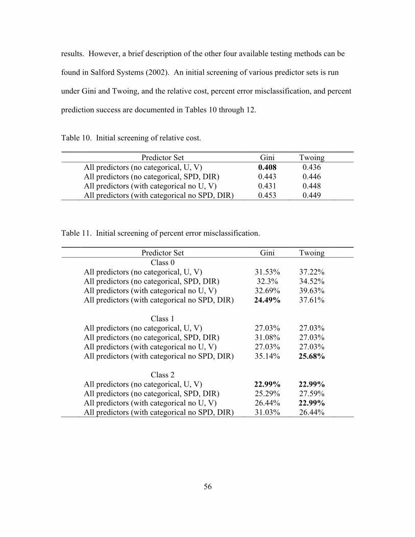
56
results. However, a brief description of the other four available testing methods can be
found in Salford Systems (2002). An initial screening of various predictor sets is run
under Gini and Twoing, and the relative cost, percent error misclassification, and percent
prediction success are documented in Tables 10 through 12.
Table 10. Initial screening of relative cost.
Predictor Set Gini Twoing All predictors (no categorical, U, V) 0.408 0.436 All predictors (no categorical, SPD, DIR) 0.443 0.446 All predictors (with categorical no U, V) 0.431 0.448 All predictors (with categorical no SPD, DIR) 0.453 0.449
Table 11. Initial screening of percent error misclassification.
Predictor Set Gini Twoing Class 0 All predictors (no categorical, U, V) 31.53% 37.22% All predictors (no categorical, SPD, DIR) 32.3% 34.52% All predictors (with categorical no U, V) 32.69% 39.63% All predictors (with categorical no SPD, DIR) 24.49% 37.61% Class 1 All predictors (no categorical, U, V) 27.03% 27.03% All predictors (no categorical, SPD, DIR) 31.08% 27.03% All predictors (with categorical no U, V) 27.03% 27.03% All predictors (with categorical no SPD, DIR) 35.14% 25.68% Class 2 All predictors (no categorical, U, V) 22.99% 22.99% All predictors (no categorical, SPD, DIR) 25.29% 27.59% All predictors (with categorical no U, V) 26.44% 22.99% All predictors (with categorical no SPD, DIR) 31.03% 26.44%

57
Table 12. Initial screening of percent prediction success.
Predictor Set Gini Twoing Class 0 All predictors (no categorical, U, V) 68.47% 62.78% All predictors (no categorical, SPD, DIR) 67.7% 65.48% All predictors (with categorical no U, V) 67.31% 60.37% All predictors (with categorical no SPD, DIR) 75.51% 62.39% Class 1 All predictors (no categorical, U, V) 72.97% 72.97% All predictors (no categorical, SPD, DIR) 68.92% 72.97% All predictors (with categorical no U, V) 72.97% 72.97% All predictors (with categorical no SPD, DIR) 64.86% 74.32% Class 2 All predictors (no categorical, U, V) 77.01% 77.01% All predictors (no categorical, SPD, DIR) 74.71% 72.41% All predictors (with categorical no U, V) 73.56% 77.01% All predictors (with categorical no SPD, DIR) 68.97% 73.56%
The relative cost of the classification model is loosely interpreted as 21 R− , in
statistical terms, or the percent of error left unexplained by the tree as compared against
the trivial model (where everything is classified under the largest class). In order to
compute relative cost (RC), Equations 18 through 20 are used
1 _ 0 _1 _ 2_ 0 _1 _ 2
misclass misclass misclassEclasses total total total
= + +
(18)
( )1 1trivialE classesclasses
= − (19)
trivial
ERCE
= (20)
where misclass_n is the number of misclassified records per Class n, and total_n is the
total of records per Class n. The overall goal is build a model where RC is very small or
close to zero. Equation 20 is minimized when there is a large number of classes, and the

58
number of misclassified records per class is small. Percent error misclassification is the
percent of the total records per Class n which are misclassified, and the percent prediction
success is one minus the percent error misclassification. Bolded values in Tables 11 and
12 are considered the best per class and method. Since each level of SPD and DIR is
computed from the U and V data at the same level, the overall predictor list is analyzed
with a SPD and DIR subset as well as a U and V subset. This separation is done to
evaluate any significance between using one version over the other; a single analysis
would use the wind-based predictors twice instead of once. In addition, categorical
(CAT) refers to unfavorable and favorable conditions of STSS and STDS.
The lowest percent error misclassification is 24.49% for Class 0, 25.68% for
Class 1, and 22.99% for Class 2. The highest prediction success is 75.51% for Class 0,
74.32% for Class 1, and 77.01% for Class 2. In this analysis, there is a split between the
Gini and Twoing methods as well as in the overall predictor set. Class 0 events have
better results with the Gini method while Class 1 events have better results with the
Twoing method. In addition, Class 2 events are split between the Gini and Twoing
methods, and the lowest relative cost occurs with the Gini method. Furthermore, the
different predictor sets are almost split evenly among the methods. This information is
illustrated in Table 13 where the counts are determined from the bolded values in Tables
10 through 12.
It appears initially that there is no way to impartially choose between the sets
without sacrificing some measure of accuracy in one or more classes. Therefore the
changes in percent error misclassification between the sets and methods are examined. If
there is minimal loss between switching to the values in one set and method over another,

59
then an overall “best” set and method can be used. In order to choose the lowest
misclassification across the classes, the average of each predictor set and method are
computed and shown in Table 14.
Table 13. Total counts of initial screening.
Predictor Set Gini Twoing All predictors (no categorical, U, V) 3 2 All predictors (no categorical, SPD, DIR) 0 0 All predictors (with categorical no U, V) 0 2 All predictors (with categorical no SPD, DIR) 2 2
Table 14. Average percent error misclassification.
Predictor Set Gini Twoing All predictors (no categorical, U, V) 27.18% 29.08% All predictors (no categorical, SPD, DIR) 29.56% 29.71% All predictors (with categorical no U, V) 28.72% 29.88% All predictors (with categorical no SPD, DIR) 30.22% 29.91%
Not surprisingly, the ranking of these results match the ranking of the relative cost
values in Table 10. Thus, the “best” predictor set is established as All predictors (no
categorical, U, V) and the “best” method is Gini. Under this determination, Class 0
events gain 7.04% error misclassification, and Class 1 events gain 1.35% error
misclassification. However, the percent error misclassification for Class 2 events
remains the same. It is important to note that these analyses are run under the assumption
that the distribution of classes in the population is equal (hence Priors Equal). This
assumption provides the most unbiased handling of the data where every record has an
equal chance of being classified in each of the target classes (Steinberg and Colla 1995
discuss each of the Priors methods available for testing). On the other hand, the

60
distribution of target classes from this population is known. Class 0 events comprise
1037 of 1198 records (~86.56%), Class 1 events comprise 74 of 1198 records (~6.18%),
and Class 2 events comprise 87 of 1198 records (~7.26%). As a result, Class 0 events are
approximately 13 times more prevalent than either Classes 1 or 2. With this
understanding, a secondary analysis is run where the actual distribution of classes is taken
into account.
After adjusting the analysis to reflect the estimated distribution frequency in each
of the classes (i.e., setting the analysis to Priors Data), the percent error misclassification
for Class 0 drops to 2.03%, and the percent error misclassification for Classes 1 and 2
rises to 68.92% and 78.16%, respectively. This analysis clearly shows that adjusting the
priors in one class can dramatically affect the outcome in another class. Steinberg and
Colla (1995) and Salford Systems (2002) suggest initially building trees under the default
of Priors Equal such that the classes are treated as if they were uniformly distributed in
the population regardless of their distribution in the sample. With an uneven distribution
of classes in this research, using Priors Equal induces a cost structure that favors a rarer
class in the data (hence Classes 1 and 2). Since it is important to provide an unbiased
assessment of the predictors in any sample (i.e., data from other years), customizing the
analysis to maximize the performance in one class is avoided, and Priors Equal is
regarded as the correct way to treat the sample.
Another way to assess predictive power without tailoring the analysis is to change
the target variable to a different predictor and compare those results against the TGT
predictor. Three other predictors (CAT STSS, CAT STDS, and CH OUT) are selected as
the target variable to see if improved percent error misclassification can be achieved.
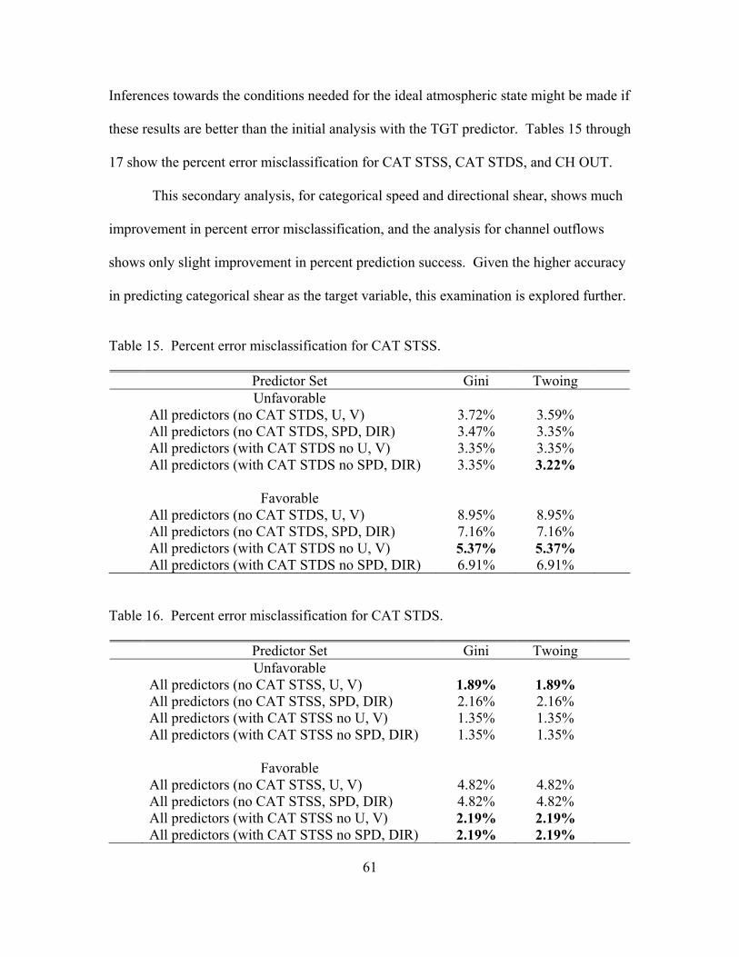
61
Inferences towards the conditions needed for the ideal atmospheric state might be made if
these results are better than the initial analysis with the TGT predictor. Tables 15 through
17 show the percent error misclassification for CAT STSS, CAT STDS, and CH OUT.
This secondary analysis, for categorical speed and directional shear, shows much
improvement in percent error misclassification, and the analysis for channel outflows
shows only slight improvement in percent prediction success. Given the higher accuracy
in predicting categorical shear as the target variable, this examination is explored further.
Table 15. Percent error misclassification for CAT STSS.
Predictor Set Gini Twoing Unfavorable All predictors (no CAT STDS, U, V) 3.72% 3.59% All predictors (no CAT STDS, SPD, DIR) 3.47% 3.35% All predictors (with CAT STDS no U, V) 3.35% 3.35% All predictors (with CAT STDS no SPD, DIR) 3.35% 3.22% Favorable All predictors (no CAT STDS, U, V) 8.95% 8.95% All predictors (no CAT STDS, SPD, DIR) 7.16% 7.16% All predictors (with CAT STDS no U, V) 5.37% 5.37% All predictors (with CAT STDS no SPD, DIR) 6.91% 6.91%
Table 16. Percent error misclassification for CAT STDS.
Predictor Set Gini Twoing Unfavorable All predictors (no CAT STSS, U, V) 1.89% 1.89% All predictors (no CAT STSS, SPD, DIR) 2.16% 2.16% All predictors (with CAT STSS no U, V) 1.35% 1.35% All predictors (with CAT STSS no SPD, DIR) 1.35% 1.35% Favorable All predictors (no CAT STSS, U, V) 4.82% 4.82% All predictors (no CAT STSS, SPD, DIR) 4.82% 4.82% All predictors (with CAT STSS no U, V) 2.19% 2.19% All predictors (with CAT STSS no SPD, DIR) 2.19% 2.19%
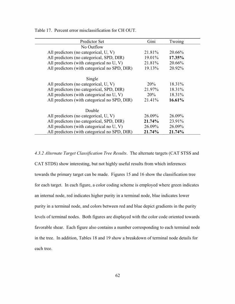
62
Table 17. Percent error misclassification for CH OUT.
Predictor Set Gini Twoing No Outflow All predictors (no categorical, U, V) 21.81% 20.66% All predictors (no categorical, SPD, DIR) 19.01% 17.35% All predictors (with categorical no U, V) 21.81% 20.66% All predictors (with categorical no SPD, DIR) 19.13% 20.92% Single All predictors (no categorical, U, V) 20% 18.31% All predictors (no categorical, SPD, DIR) 21.97% 18.31% All predictors (with categorical no U, V) 20% 18.31% All predictors (with categorical no SPD, DIR) 21.41% 16.61% Double All predictors (no categorical, U, V) 26.09% 26.09% All predictors (no categorical, SPD, DIR) 21.74% 23.91% All predictors (with categorical no U, V) 26.09% 26.09% All predictors (with categorical no SPD, DIR) 21.74% 21.74%
4.3.2 Alternate Target Classification Tree Results. The alternate targets (CAT STSS and
CAT STDS) show interesting, but not highly useful results from which inferences
towards the primary target can be made. Figures 15 and 16 show the classification tree
for each target. In each figure, a color coding scheme is employed where green indicates
an internal node, red indicates higher purity in a terminal node, blue indicates lower
purity in a terminal node, and colors between red and blue depict gradients in the purity
levels of terminal nodes. Both figures are displayed with the color code oriented towards
favorable shear. Each figure also contains a number corresponding to each terminal node
in the tree. In addition, Tables 18 and 19 show a breakdown of terminal node details for
each tree.
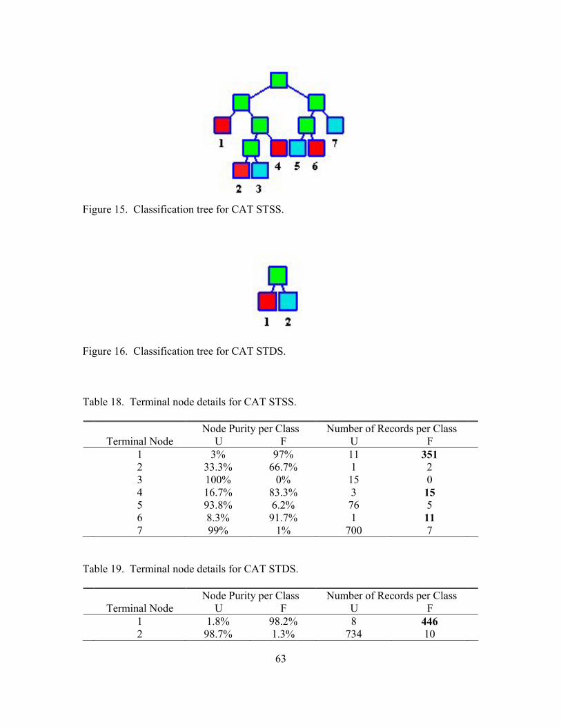
63
Figure 15. Classification tree for CAT STSS.
Figure 16. Classification tree for CAT STDS.
Table 18. Terminal node details for CAT STSS.
Terminal Node
Node Purity per Class U F
Number of Records per Class U F
1 3% 97% 11 351 2 33.3% 66.7% 1 2 3 100% 0% 15 0 4 16.7% 83.3% 3 15 5 93.8% 6.2% 76 5 6 8.3% 91.7% 1 11 7 99% 1% 700 7
Table 19. Terminal node details for CAT STDS.
Terminal Node
Node Purity per Class U F
Number of Records per Class U F
1 1.8% 98.2% 8 446 2 98.7% 1.3% 734 10

64
The highest purity terminal nodes for CAT STSS are Node 1 with 351 records,
Node 4 with 15 records, and Node 6 with 11 records. An examination of the splitting
rules for each node is portrayed in Table 20. The highest purity terminal node for CAT
STDS is Node 1 with 446 records; the splitting rules for this node are found in Table 21.
Table 20. Splitting rules for CAT STSS.
Terminal Node Splitting Rules 1 TTSS < 15.825
4
CAT STDS is favorable && TTSS > 15.825 &&
TTSS < 16.16
6
TTSS > 16.61 && TTSS < 18.79 && E50 SPD > 31.92
Table 21. Splitting rules for CAT STDS.
Terminal Node Splitting Rules 1 TTDS < 44.965
Although the purity levels are high for each target variable, the amount of information
gleaned from the splitting rules is minimal. Only one terminal node in each target
contains a substantial quantity of records despite other nodes (within CAT STSS) having
purity levels in excess of 80%. However, this limitation should not be discarded all
together. The analysis confirms JTWC’s guidance on speed and directional shear
(i.e., 15 kts and 45 deg for favorable conditions), and the levels needed to compute shear
can now be extended to 1000-200 mb versus only examining surface-200 mb. These
results are helpful if there is high confidence in predicting rapid intensification and

65
weakening based on TTSS and TTDS. Otherwise, inferring changes based on the
alternate target variables (CAT STSS, CAT STDS, and CH OUT) do not provide
significant impact to the forecast process. The results based on the primary target are
illustrated in greater depth in the next section.
4.3.3 Primary Target Classification Tree Results. An initial examination of the primary
target results yields a wide variety of terminal nodes. Figures 17 through 19 show the
color coding scheme based on Classes 2, 1, and 0. This color scheme is exactly the same
as discussed in the previous section. These figures illustrate that the highest
concentration of purity in the tree is focused towards Class 0 events. Class 1 and 2 events
comprise a much smaller concentration of purity within the overall structure. Terminal
node details for the TGT tree are found in Table 22.
Another useful examination of the TGT tree can be found in the variable
importance table. This table shows the hierarchy of predictor importance with respect to
improvement scores. During the tree building process, each predictor is examined as the
primary splitter, and the improvement score associated with that split is kept in memory.
Once the optimal tree is grown, the improvement scores are summed over all predictors,
the most important predictor receiving a score of 100. Every predictor listed below the
top variable has a score which is considered a certain fraction of importance to the overall
tree building process. The variable importance table for the TGT tree is portrayed in
Table 23.
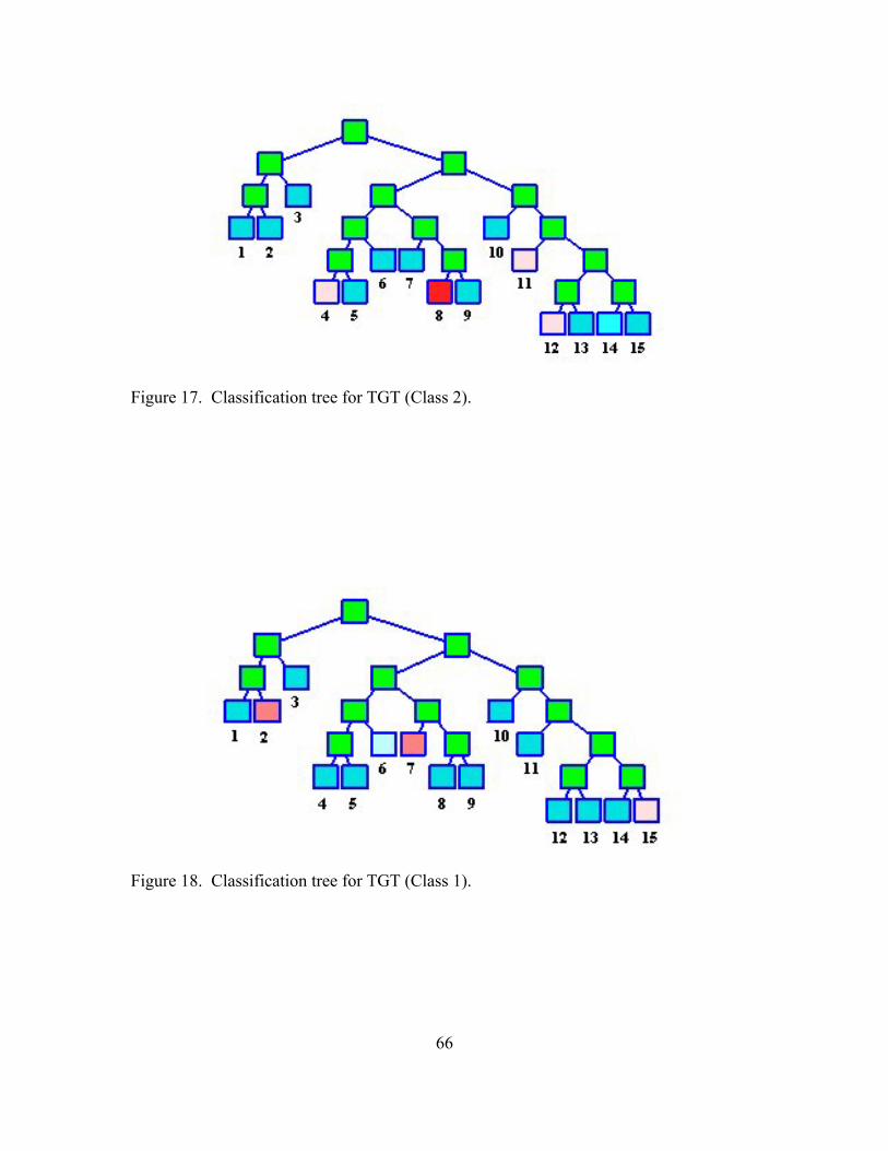
66
Figure 17. Classification tree for TGT (Class 2).
Figure 18. Classification tree for TGT (Class 1).
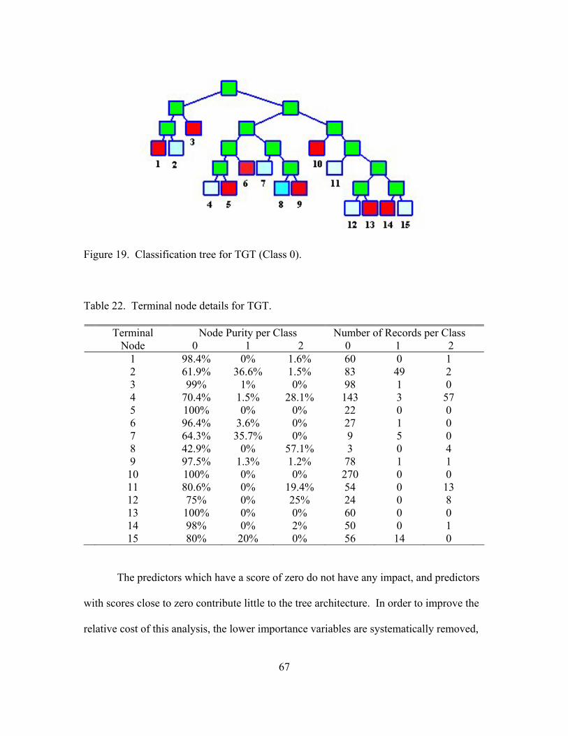
67
Figure 19. Classification tree for TGT (Class 0).
Table 22. Terminal node details for TGT.
Terminal Node
Node Purity per Class 0 1 2
Number of Records per Class 0 1 2
1 98.4% 0% 1.6% 60 0 1 2 61.9% 36.6% 1.5% 83 49 2 3 99% 1% 0% 98 1 0 4 70.4% 1.5% 28.1% 143 3 57 5 100% 0% 0% 22 0 0 6 96.4% 3.6% 0% 27 1 0 7 64.3% 35.7% 0% 9 5 0 8 42.9% 0% 57.1% 3 0 4 9 97.5% 1.3% 1.2% 78 1 1 10 100% 0% 0% 270 0 0 11 80.6% 0% 19.4% 54 0 13 12 75% 0% 25% 24 0 8 13 100% 0% 0% 60 0 0 14 98% 0% 2% 50 0 1 15 80% 20% 0% 56 14 0
The predictors which have a score of zero do not have any impact, and predictors
with scores close to zero contribute little to the tree architecture. In order to improve the
relative cost of this analysis, the lower importance variables are systematically removed,

68
and a new tree is grown. It is important to note that removing too many predictors can
actually result in a higher relative cost. Thus, there is an optimal set of predictors which
should be used to minimize the relative cost and overall misclassification rate. After
analyzing multiple predictor sets, the variables associated with the lowest overall relative
cost are displayed in Table 24.
This particular set of predictors yields a relative cost of 0.322 with a
misclassification rate of 29.12% for Class 0, 13.51% for Class 1, and 21.84% for Class 2.
When these results are compared to the initial screening results, the absolute change in
misclassification rate is +4.63% for Class 0, -12.17% for Class 1, and -1.15% for Class 2.
Therefore, it is clear that a substantial gain in predictability is achieved for rapidly
weakening events, and a slight gain in predictability is achieved for rapidly intensifying
events. However, the improvement in both of these classes comes at a slight increase in
the misclassification of events where no rapid change is occurring. Since the majority of
focus should be placed upon an environment conducive to rapid change versus a more
stagnant or slowly changing environment, these results are insightful. If misclassification
is thought of in terms of false alarm rate, using the refined list of predictors (or list of
critical predictors) should yield 70.88% accuracy in predicting typhoon rapid
intensification and 86.49% accuracy in predicting typhoon rapid weakening. In order to
visualize these results, Figures 20 through 22 show the new classification trees per focus
class, and Figure 23 shows the splitter at each internal node.
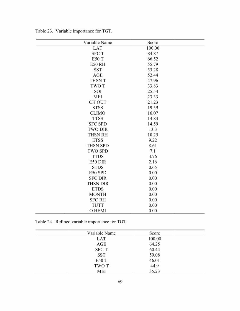
69
Table 23. Variable importance for TGT.
Variable Name Score LAT 100.00 SFC T 84.87 E50 T 66.52 E50 RH 55.79 SST 53.28 AGE 52.44 THSN T 47.96 TWO T 33.83 SOI 25.54 MEI 23.33 CH OUT 21.23 STSS 19.59 CLIMO 16.07 TTSS 14.84 SFC SPD 14.59 TWO DIR 13.3 THSN RH 10.25 ETSS 9.22 THSN SPD 8.61 TWO SPD 7.1 TTDS 4.76 E50 DIR 2.16 STDS 0.65 E50 SPD 0.00 SFC DIR 0.00 THSN DIR 0.00 ETDS 0.00 MONTH 0.00 SFC RH 0.00 TUTT 0.00 O HEMI 0.00
Table 24. Refined variable importance for TGT.
Variable Name Score LAT 100.00 AGE 64.25 SFC T 60.44 SST 59.08 E50 T 46.01 TWO T 44.9 MEI 35.23
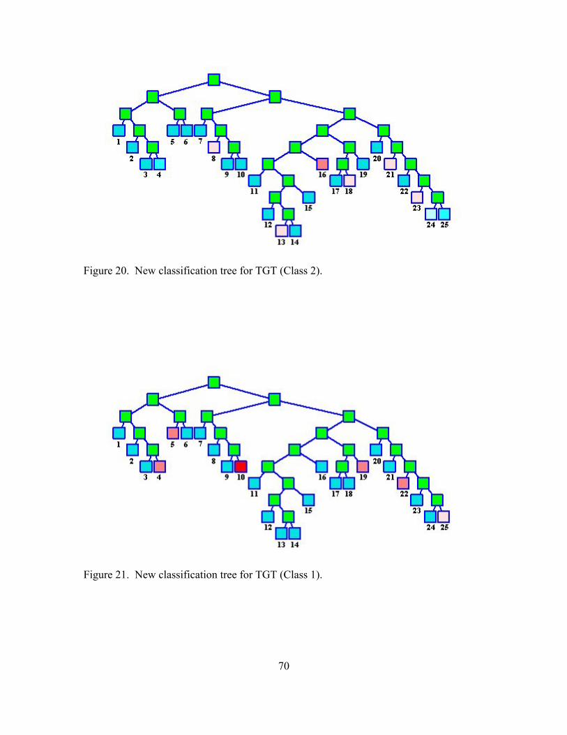
70
Figure 20. New classification tree for TGT (Class 2).
Figure 21. New classification tree for TGT (Class 1).
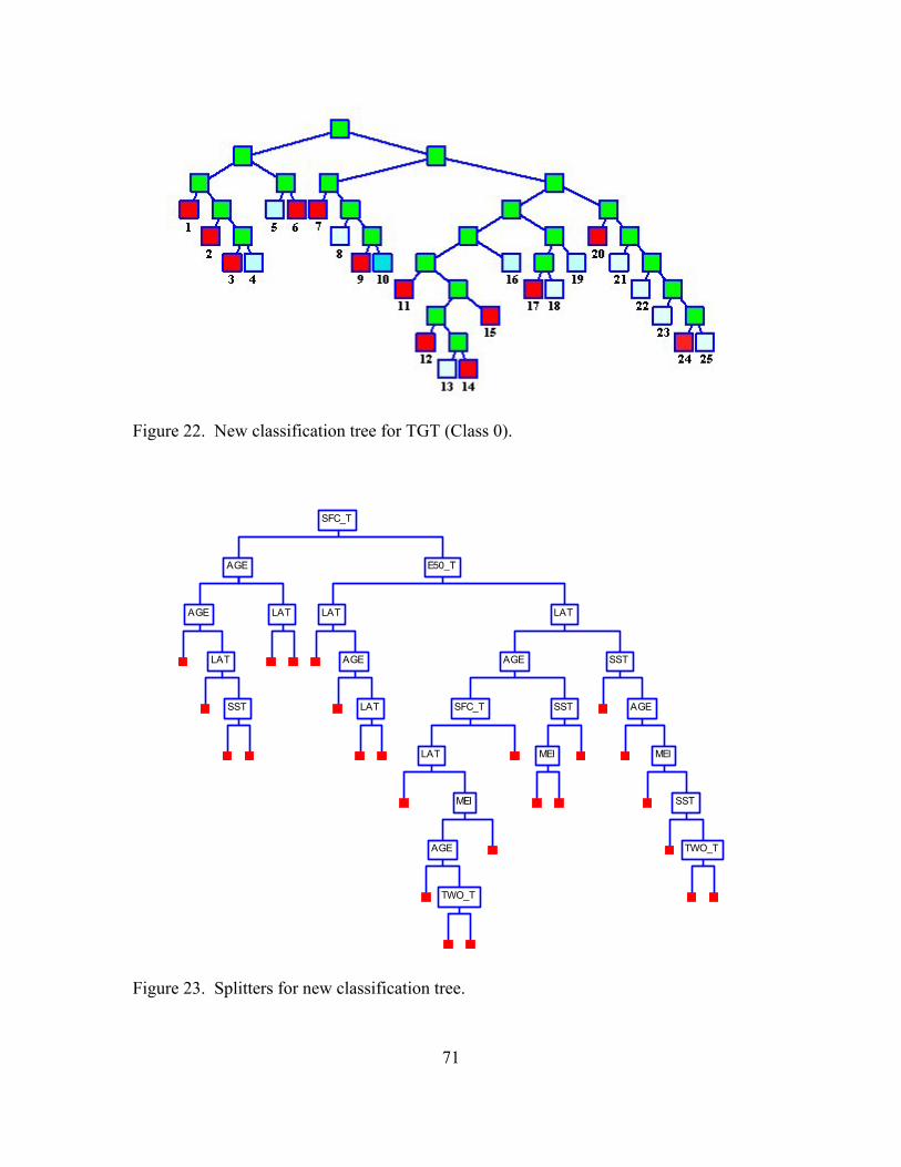
71
Figure 22. New classification tree for TGT (Class 0).
SST
LAT
AGE
LAT
AGE
LAT
AGE
LAT
TWO_T
AGE
MEI
LAT
SFC_T
MEI
SST
AGE
TWO_T
SST
MEI
AGE
SST
LAT
E50_T
SFC_T
Figure 23. Splitters for new classification tree.

72
Similar to Figures 17 through 19, the highest concentration of purity in the tree is
focused towards Class 0 events. Class 1 and 2 events comprise a much smaller amount
of homogeneity within the overall structure. The new terminal node details are found in
Table 25. This table shows a relatively even distribution of Class 0 records in each of the
terminal nodes, except for Node 7 which has 206 records. Class 1 records are located
mainly in Node 4 while the largest quantity of Class 2 records are dispersed between
Nodes 13, 16, and 19. Since the primary focus is towards predicting Class 1 and 2
events, and these events are not situated in the same terminal nodes, an examination of
the splitting rules is accomplished. Table 26 shows the splitting rules for each of the
nodes which have the greatest number of records in Class 1 and 2. This examination is
done to determine the highest occurrence of the same rule or type of rule. For example, if
a criteria is split on a certain value, it is essential to draw this information out and
examine it based on meteorological soundness.
The summation of records in Table 26 is 71 for Class 1 and 73 for Class 2. This
number represents 95.95% and 83.91% of the total number available in each class,
respectively. Table 26 also denotes the largest groups of records in each class from Table
25 (bolded values). The remaining records in Table 25 are few and dispersed among the
rest of the terminal nodes. In order to develop a concise forecast decision tree, the nodes
with only a couple of records are not reflected in Table 26. However, the splitting rules
for the entire tree (i.e., across all terminal nodes) can be found in Appendix C.
Given the variety of splitting rules in Table 26, it is crucial to evaluate each one
based on meteorological soundness. For example, the splitting rules for SFC T in Class 1
events (rapid weakening) show SFC T > 26.89 and SFC T < 26.89. Only one of these
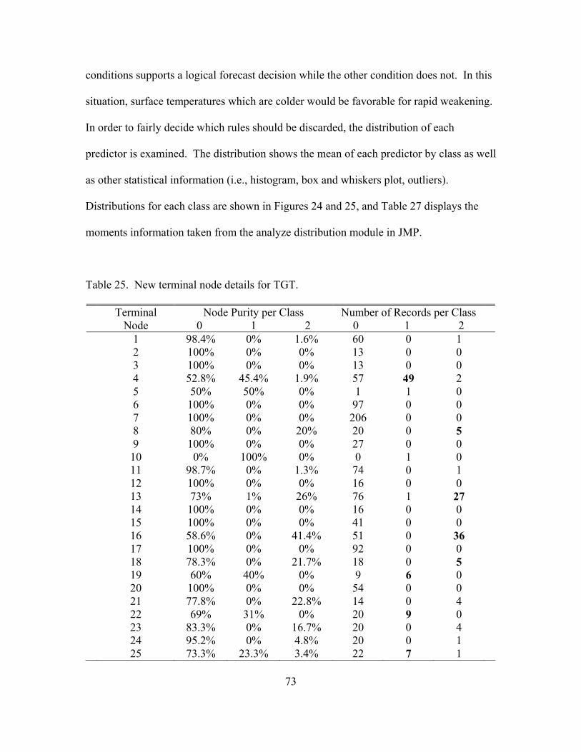
73
conditions supports a logical forecast decision while the other condition does not. In this
situation, surface temperatures which are colder would be favorable for rapid weakening.
In order to fairly decide which rules should be discarded, the distribution of each
predictor is examined. The distribution shows the mean of each predictor by class as well
as other statistical information (i.e., histogram, box and whiskers plot, outliers).
Distributions for each class are shown in Figures 24 and 25, and Table 27 displays the
moments information taken from the analyze distribution module in JMP.
Table 25. New terminal node details for TGT.
Terminal Node
Node Purity per Class 0 1 2
Number of Records per Class 0 1 2
1 98.4% 0% 1.6% 60 0 1 2 100% 0% 0% 13 0 0 3 100% 0% 0% 13 0 0 4 52.8% 45.4% 1.9% 57 49 2 5 50% 50% 0% 1 1 0 6 100% 0% 0% 97 0 0 7 100% 0% 0% 206 0 0 8 80% 0% 20% 20 0 5 9 100% 0% 0% 27 0 0 10 0% 100% 0% 0 1 0 11 98.7% 0% 1.3% 74 0 1 12 100% 0% 0% 16 0 0 13 73% 1% 26% 76 1 27 14 100% 0% 0% 16 0 0 15 100% 0% 0% 41 0 0 16 58.6% 0% 41.4% 51 0 36 17 100% 0% 0% 92 0 0 18 78.3% 0% 21.7% 18 0 5 19 60% 40% 0% 9 6 0 20 100% 0% 0% 54 0 0 21 77.8% 0% 22.8% 14 0 4 22 69% 31% 0% 20 9 0 23 83.3% 0% 16.7% 20 0 4 24 95.2% 0% 4.8% 20 0 1 25 73.3% 23.3% 3.4% 22 7 1
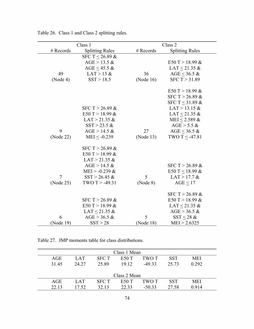
74
Table 26. Class 1 and Class 2 splitting rules.
Class 1 Class 2 # Records Splitting Rules # Records Splitting Rules
49 (Node 4)
SFC T < 26.89 & AGE > 13.5 & AGE < 45.5 & LAT > 13 & SST > 18.5
36 (Node 16)
E50 T > 18.99 & LAT < 21.35 & AGE < 36.5 & SFC T > 31.89
9
(Node 22)
SFC T > 26.89 & E50 T > 18.99 & LAT > 21.35 & SST > 23.5 & AGE > 14.5 & MEI < -0.239
27 (Node 13)
E50 T > 18.99 & SFC T > 26.89 & SFC T < 31.89 & LAT > 13.15 & LAT < 21.35 & MEI < 2.589 & AGE > 5.5 & AGE < 36.5 &
TWO T < -47.81
7
(Node 25)
SFC T > 26.89 & E50 T > 18.99 & LAT > 21.35 & AGE > 14.5 &
MEI > -0.239 & SST > 26.45 &
TWO T > -49.31
5
(Node 8)
SFC T > 26.89 & E50 T < 18.99 &
LAT > 17.7 & AGE < 17
6
(Node 19)
SFC T > 26.89 & E50 T > 18.99 & LAT < 21.35 & AGE > 36.5 &
SST > 28
5
(Node 18)
SFC T > 26.89 & E50 T > 18.99 & LAT < 21.35 & AGE > 36.5 &
SST < 28 & MEI > 2.6325
Table 27. JMP moments table for class distributions.
Class 1 Mean AGE LAT SFC T E50 T TWO T SST MEI 31.45 24.27 25.89 19.12 -49.33 25.73 0.292
Class 2 Mean
AGE LAT SFC T E50 T TWO T SST MEI 22.13 17.52 32.13 22.33 -50.33 27.58 0.914
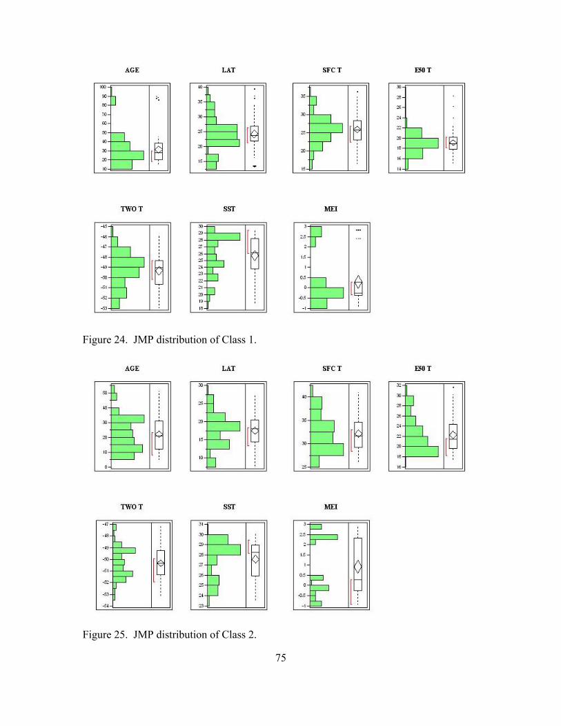
75
Figure 24. JMP distribution of Class 1.
Figure 25. JMP distribution of Class 2.

76
The mean of each predictor is used as a threshold for determining the
meteorological soundness of the CART splitting rule. Since there are instances of
conflicting conditions, the mean provides the basis to further refine the splitting rule.
Additionally, if the splitting rule is not consistent with the predictor mean, it should be
discarded. For example, the splitting rule might suggest a criteria which would not be
expected meteorologically (e.g., cold temperatures for rapid intensification). However, if
the splitting rule makes logical sense, it should be kept.
The criteria established in Table 28 are the average of the means of the predictor
in each class according to distributions in Table 27. The mean is used such that if the
splitting rule meets these criteria (i.e., the mean brings the splitting rule “into
agreement”), then conditions are favorable for that class. If the splitting rule does not
meet these criteria, then conditions are deemed unfavorable, and the rule should be
discarded. The values do not incorporate the effects of Class 0 events because the
objective is to determine the validity of a splitting rule for Class 1 and 2 events. The
rationale for using the criteria in Table 28 is described as follows:
AGE: Rapid intensification more favorable during earlier stage in lifecycle. LAT: Rapid intensification more favorable in lower latitudes. SFC T: Rapid intensification more favorable with warmer temperatures. E50 T: Rapid intensification more favorable with warmer temperatures. TWO T: Rapid intensification more favorable with warmer temperatures. SST: Rapid intensification more favorable with warmer temperatures. MEI: Rapid intensification more favorable with positive values.
A typhoon has more time to develop in the earlier stages of the lifecycle than it does in
the later stage of the lifecycle. Also, typhoons which reside in lower latitudes are not
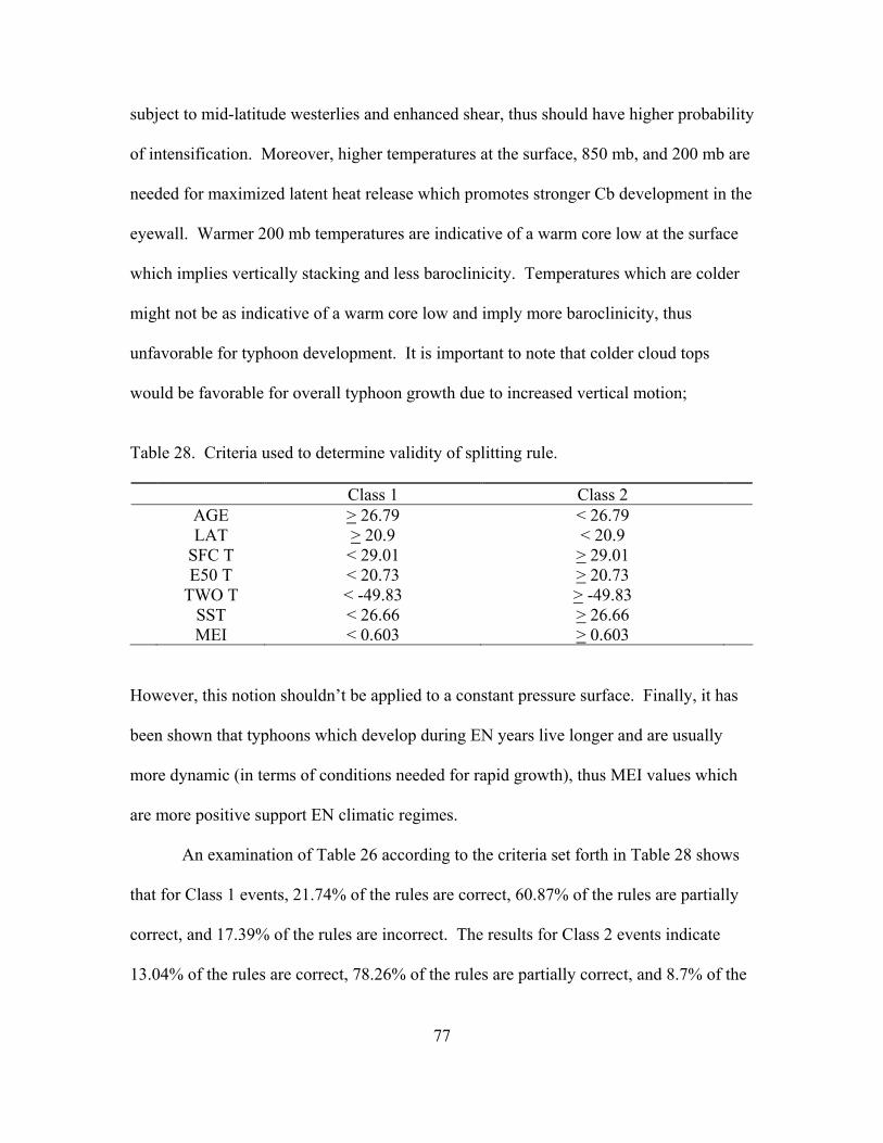
77
subject to mid-latitude westerlies and enhanced shear, thus should have higher probability
of intensification. Moreover, higher temperatures at the surface, 850 mb, and 200 mb are
needed for maximized latent heat release which promotes stronger Cb development in the
eyewall. Warmer 200 mb temperatures are indicative of a warm core low at the surface
which implies vertically stacking and less baroclinicity. Temperatures which are colder
might not be as indicative of a warm core low and imply more baroclinicity, thus
unfavorable for typhoon development. It is important to note that colder cloud tops
would be favorable for overall typhoon growth due to increased vertical motion;
Table 28. Criteria used to determine validity of splitting rule.
Class 1 Class 2 AGE > 26.79 < 26.79 LAT > 20.9 < 20.9 SFC T < 29.01 > 29.01 E50 T < 20.73 > 20.73 TWO T < -49.83 > -49.83 SST < 26.66 > 26.66 MEI < 0.603 > 0.603
However, this notion shouldn’t be applied to a constant pressure surface. Finally, it has
been shown that typhoons which develop during EN years live longer and are usually
more dynamic (in terms of conditions needed for rapid growth), thus MEI values which
are more positive support EN climatic regimes.
An examination of Table 26 according to the criteria set forth in Table 28 shows
that for Class 1 events, 21.74% of the rules are correct, 60.87% of the rules are partially
correct, and 17.39% of the rules are incorrect. The results for Class 2 events indicate
13.04% of the rules are correct, 78.26% of the rules are partially correct, and 8.7% of the
78
rules are incorrect. The rules which are partially correct contain a range of values where
the threshold does and does not apply. For example, in Terminal Node 4, the splitting
rule for AGE is > 13.5 & < 45.5. This rule is partially correct since the threshold criteria
for AGE is > 26.79. Since the majority of the splitting rules are deemed only partially
correct (in agreement with the predictor means), it is essential for the forecaster to use
experience and sound judgment in determining applicability of the rule. The only
guideline in determining correct or incorrect rules is the arithmetic mean of the class
distribution. However, it is encouraging to see 82.61% of Class 1 and 91.3% of Class 2
events denoted as either correct or partially correct. These percentages show high
confidence in determining intensification trends.
4.4 Supplement to the Intensity Analysis Worksheet and Verification
The intensity analysis worksheet, shown in Table 29, reflects parameters that
JTWC uses along with model consensus forecasting. The criteria are dominant in Dvorak
analysis as well as satellite interpretation. In addition, the worksheet incorporates
changes in sea surface temperatures as well as interactions with outflow channels and
TUTT cells. However, this intensity analysis does not include NOGAPS model output.
The inclusion of model data is most likely dictated by the consensus forecasting
technique. Since the majority of the parameters in Table 29 are not utilized in the CART
analysis, they are still considered important features to the TC forecast process. In
addition to these parameters, the forecast guidance in Table 30 is suggested as a
supplement. This forecast guidance incorporates the correct and partially correct splitting
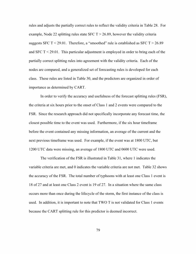
79
rules and adjusts the partially correct rules to reflect the validity criteria in Table 28. For
example, Node 22 splitting rules state SFC T > 26.89, however the validity criteria
suggests SFC T < 29.01. Therefore, a “smoothed” rule is established as SFC T > 26.89
and SFC T < 29.01. This particular adjustment is employed in order to bring each of the
partially correct splitting rules into agreement with the validity criteria. Each of the
nodes are compared, and a generalized set of forecasting rules is developed for each
class. These rules are listed in Table 30, and the predictors are organized in order of
importance as determined by CART.
In order to verify the accuracy and usefulness of the forecast splitting rules (FSR),
the criteria at six hours prior to the onset of Class 1 and 2 events were compared to the
FSR. Since the research approach did not specifically incorporate any forecast time, the
closest possible time to the event was used. Furthermore, if the six hour timeframe
before the event contained any missing information, an average of the current and the
next previous timeframe was used. For example, if the event was at 1800 UTC, but
1200 UTC data were missing, an average of 1800 UTC and 0600 UTC were used.
The verification of the FSR is illustrated in Table 31, where 1 indicates the
variable criteria are met, and 0 indicates the variable criteria are not met. Table 32 shows
the accuracy of the FSR. The total number of typhoons with at least one Class 1 event is
18 of 27 and at least one Class 2 event is 19 of 27. In a situation where the same class
occurs more than once during the lifecycle of the storm, the first instance of the class is
used. In addition, it is important to note that TWO T is not validated for Class 1 events
because the CART splitting rule for this predictor is deemed incorrect.
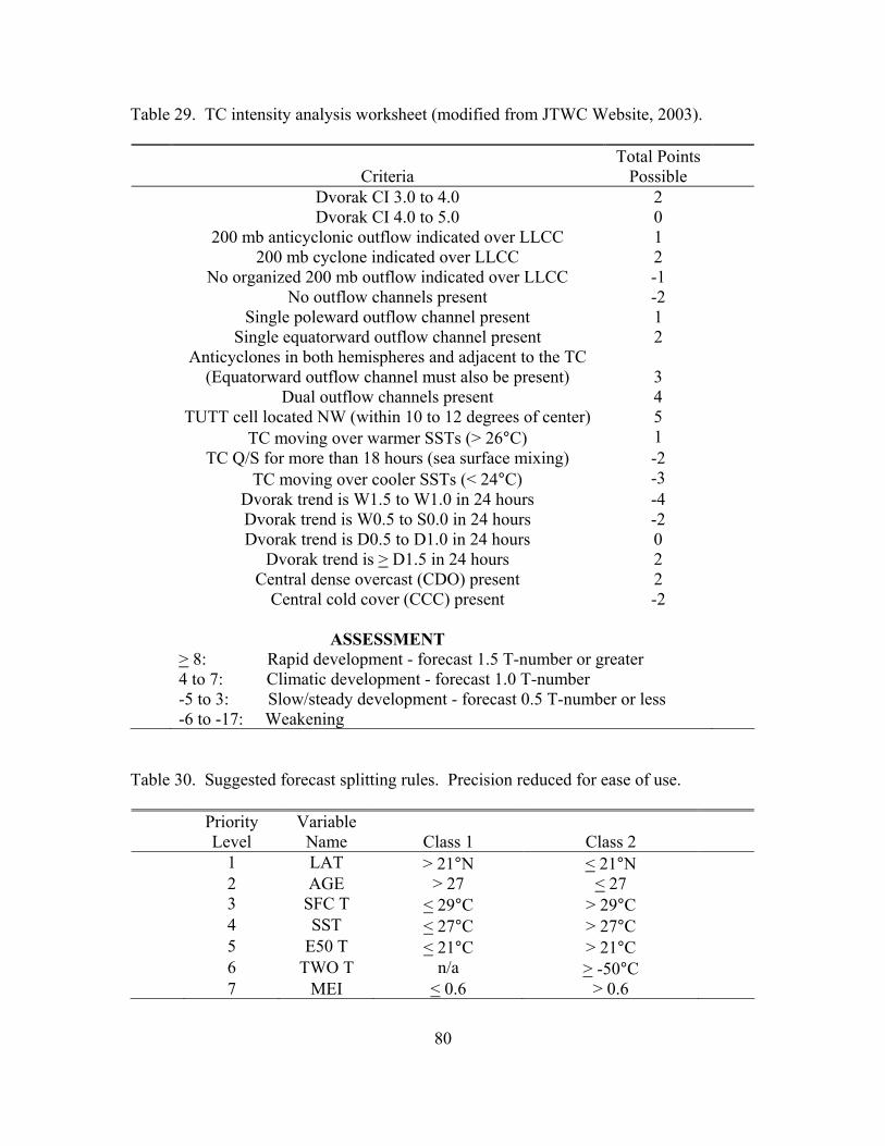
80
Table 29. TC intensity analysis worksheet (modified from JTWC Website, 2003).
Criteria
Total Points Possible
Dvorak CI 3.0 to 4.0 2 Dvorak CI 4.0 to 5.0 0 200 mb anticyclonic outflow indicated over LLCC 1 200 mb cyclone indicated over LLCC 2 No organized 200 mb outflow indicated over LLCC -1 No outflow channels present -2 Single poleward outflow channel present 1 Single equatorward outflow channel present 2 Anticyclones in both hemispheres and adjacent to the TC
(Equatorward outflow channel must also be present) 3
Dual outflow channels present 4 TUTT cell located NW (within 10 to 12 degrees of center) 5 TC moving over warmer SSTs (> 26°C) 1 TC Q/S for more than 18 hours (sea surface mixing) -2 TC moving over cooler SSTs (< 24°C) -3 Dvorak trend is W1.5 to W1.0 in 24 hours -4 Dvorak trend is W0.5 to S0.0 in 24 hours -2 Dvorak trend is D0.5 to D1.0 in 24 hours 0 Dvorak trend is > D1.5 in 24 hours 2 Central dense overcast (CDO) present 2 Central cold cover (CCC) present -2 ASSESSMENT > 8: Rapid development - forecast 1.5 T-number or greater
4 to 7: Climatic development - forecast 1.0 T-number -5 to 3: Slow/steady development - forecast 0.5 T-number or less -6 to -17: Weakening
Table 30. Suggested forecast splitting rules. Precision reduced for ease of use.
Priority Level
Variable Name
Class 1
Class 2
1 LAT > 21°N < 21°N 2 AGE > 27 < 27 3 SFC T < 29°C > 29°C 4 SST < 27°C > 27°C 5 E50 T < 21°C > 21°C 6 TWO T n/a > -50°C 7 MEI < 0.6 > 0.6
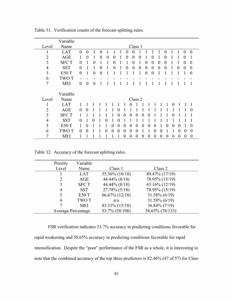
81
Table 31. Verification counts of the forecast splitting rules.
Level Variable
Name
Class 1
1 LAT 0 0 1 0 1 1 1 0 0 1 1 1 1 0 1 1 0 0 2 AGE 1 0 1 0 0 0 1 0 0 0 1 0 1 0 1 1 0 1 3 SFC T 0 1 0 1 1 0 1 1 0 1 0 0 0 0 1 1 0 0 4 SST 0 1 1 0 1 0 1 0 0 0 0 0 0 0 1 0 0 0 5 E50 T 0 1 0 0 1 1 1 1 1 1 0 0 1 1 1 1 1 0 6 TWO T - - - - - - - - - - - - - - - - - - 7 MEI 0 0 0 1 1 1 1 1 1 1 1 1 1 1 1 1 1 1
Level Variable
Name
Class 2
1 LAT 1 1 1 1 1 1 1 1 0 1 1 1 1 1 1 0 1 1 1 2 AGE 0 0 1 1 1 1 0 1 1 1 1 1 1 1 1 1 1 1 0 3 SFC T 1 1 1 1 1 1 0 0 0 0 0 0 1 1 1 0 1 1 1 4 SST 0 1 0 1 0 1 0 1 1 1 1 1 1 1 1 1 1 1 1 5 E50 T 1 0 1 1 1 0 0 0 0 0 0 0 0 1 0 0 0 1 0 6 TWO T 0 0 1 1 0 0 0 0 0 0 1 1 0 0 1 1 0 0 0 7 MEI 1 1 1 1 1 1 1 0 0 0 0 0 0 0 0 0 0 0 0
Table 32. Accuracy of the forecast splitting rules.
Priority Level
Variable Name
Class 1
Class 2
1 LAT 55.56% (10/18) 89.47% (17/19) 2 AGE 44.44% (8/18) 78.95% (15/19) 3 SFC T 44.44% (8/18) 63.16% (12/19) 4 SST 27.78% (5/18) 78.95% (15/19) 5 E50 T 66.67% (12/18) 31.58% (6/19) 6 TWO T n/a 31.58% (6/19) 7 MEI 83.33% (15/18) 36.84% (7/19) Average Percentage 53.7% (58/108) 58.65% (78/133)
FSR verification indicates 53.7% accuracy in predicting conditions favorable for
rapid weakening and 58.65% accuracy in predicting conditions favorable for rapid
intensification. Despite the “poor” performance of the FSR as a whole, it is interesting to
note that the combined accuracy of the top three predictors is 82.46% (47 of 57) for Class

82
2 events and 68.52% (37 of 54) for Class 1 events. The predictors in Class 2 comprise
priority levels 1, 2, and 4 while the predictors in Class 1 comprise priority levels 7, 5, and
1. This comparison suggests the priority levels should be redefined based on FSR
accuracy rather than the CART variable importance table. The predictors (in order of
importance) which should be given the most weight are LAT, AGE, and SST for Class 2
and MEI, E50 T, and LAT for Class 1. The other predictors in each class shouldn’t
necessarily be disregarded, however the predictive power might not be as great.
The rules established in Table 30 are only suggestions based on a combination of
CART analysis splitting rules and validity criteria. An analyst still needs to use
discretion while taking the FSR and the intensity analysis worksheet into consideration.
In addition, not all of the rules are required for each forecasting scenario since not every
predictor was used in each of the nodes listed in Table 26. Sound forecast judgment
should prevail when opting to utilize one, two, or all of these rules. Furthermore, these
rules are based on an exact split criteria, and this particular value can be adjusted given
the environmental conditions present. If only a proportion of the suggested FSR is used,
more weight should be given to the higher accuracy variables.
These rules are verified at the closest timeframe to the event occurring (i.e., six
hours before intensification and weakening). Given the potential variability in the model
parameters at some time in the future, it is probable that not all of the criteria will be met
at the same time or over the same location. These rules are formulated as suggestive
criteria, and forecaster judgment must always take higher priority. However, despite the
70% to 80% levels of accuracy, the rules shed light as to which model parameters have
more predictive power, and they provide an enhancement to the forecast process.

83
V. Conclusions and Recommendations
5.1 Conclusions
The overall goal of this research was to data mine atmospheric parameters
responsible for typhoon rapid intensification and weakening and to validate the
usefulness of using these parameters in the forecast process. The primary method used to
meet this goal was classification tree analyses. This research used components of the
NOGAPS model along with numerous other atmospheric and climatic predictors. In
addition to this examination, several minor objectives listed in Section 1.2 were also
achieved.
The first objective was to gather all types of satellite imagery (visible, water
vapor, and infrared) since satellite interrogation has become one of the primary tools in
analyzing Northwest Pacific typhoons. Due to the availability of data covering the areas
of interest, only infrared imagery from the Australian BOM was used. The data from the
NRL did not provide enough of a synoptic-scale view to glean the necessary information.
The infrared imagery provided a means of determining channel outflow patterns and
when used with archived model fields from NCEP, interactions with TUTT cells and
opposite hemispheric effects were verified.
The second objective was to collect the BT data which were obtained from
JTWC. These data were vital in establishing the specific times associated with rapid
weakening and intensification events (Class 1 and 2 events). The BT data also provided
the specific timelines from which to gather NOGAPS model fields (objective 3). Each of
84
the records in the database were time matched with specific model data as well as
subjective calls in the form of binary responses (0 for “no” and 1 for “yes”).
Temperature, relative humidity, and wind components (U and V) were the primary fields
used from the NOGAPS model. The U and V components established speed and
directional shear at different levels.
Inclusion of climatological effects comprised the fourth objective of the research.
The early hypothesis that EN and LN regimes might have some influence on
intensification trends was verified in this work. Furthermore, relationships between
TUTT cells and climatic regimes were established. Although none of the 1999 storms
had any interactions with the TUTT, both the 1997 and 2001 seasons showed typhoons
which interacted with tropical upper level troughs.
The final objective was to examine relationships between the various predictors
by using CART analyses. Since the target variable was defined categorically, a
classification analysis was utilized. However, simple linear regression was used to
compare the NOGAPS analyses of surface wind speed to the BT surface wind speeds.
The classification analyses revealed interesting relationships between the target variable
and the predictors. Some of the predictors, which were initially thought to play a vital
role (such as speed, directional shear, and channel outflows) were revealed as less
important, and some of the predictors which were not initially considered important
became key players in the architecture of the classification tree importance. Nonetheless,
it was a synergy of seven predictors (AGE, LAT, SFC T, E50 T, TWO T, SST, and MEI)
which shed new light into when and under what conditions typhoons seem to intensify.

85
Using classification analyses to determine tropical cyclone intensification trends
is feasible. The results, while not excellent at present, are promising in the data mining
process. The original tree contains a percent error misclassification of 24.49% for Class
0, 25.68% for Class 1, and 22.99% for Class 2 events. After refining the predictor list (by
systematically removing weaker predictors, which increase the relative cost), the percent
error misclassifications become 29.12% for Class 0, 13.51% for Class 1, and 21.84% for
Class 2 events. These new percentages are slightly different than the percent accuracy
found in the verification process.
The verification process used the FSR as a basis for determining Class 1 and
Class 2 events. The FSR as a whole showed an accuracy of 53.7% for Class 1 and
58.65% in Class 2 events. Verification in Class 0 was not done because this class
represented neither rapid intensification nor rapid weakening (i.e., not one of the classes
of interest). In addition to the complete FSR accuracy, the top three predictors in each
class yielded 68.52% accuracy for Class 1 and 82.46% accuracy for Class 2 events.
In essence, the percent error misclassification and the FSR verification represent
two different measures of the classification tree feasibility. The misclassification rates
demonstrate the ability of the tree to accurately filter each of the classes into terminal
nodes with the proper class assignments. The verification process characterizes the
accuracy of using each parameter in the FSR against the actual events. Since neither set
of percentages (misclassification nor verification) show a dominating level of accuracy,
the overall performance of the CART model is deemed valid. If these percentages had
been above 80% (which assumes a 20% false alarm rate), then the model would be
86
considered excellent. However, the false alarm level is strictly user organization directed
and dependent on the DoD assets at each operating location.
In addition to the results from the primary target classification trees, the alternate
target classification trees (CH OUT, CAT STSS, and CAT STDS) showed interesting
outcomes. Categorical speed and directional shear as well as channel outflows were also
considered as target variables. Although the channel outflow predictor did not yield
results which were better than the primary target, categorical shear confirmed the criteria
JTWC uses for favorable and unfavorable conditions. It was shown that the criteria of 15
kts and 45 degrees of shear can be now applied to the 1000-200 mb level versus only the
surface-200 mb level. This validation provides an increase in the understanding of the
intricacies of tropical cyclone intensification.
5.2 Recommendations
5.2.1 Recommendations to JTWC. CART analyses provide insightful information based
on large databases and a variety of predictors. However, given the unique nature of the
data mining process, the analyses provide a set of trees with varying degrees of size and
accuracy (percent error misclassification and prediction success). In this research, the
optimal tree, which minimized the percent error misclassification across all of the classes,
was comprised of 25 terminal nodes. In addition, the splitting rules which led to the 25
terminal nodes varied among seven predictors, and the splitting rule path for each
terminal node was unique. Although this technique was powerful in extracting every
possible split in the data to produce a forecast decision path, it did not provide a concise

87
set of rules. Therefore, a generalization of the splitting rules was made, and a suggested
set of splitting rules was established based on target class. This suggested set focused
heavily on the CART analyses, however it still relies on sound meteorology when a
CART split is considered unrealistic. The decision to utilize a CART splitting rule is
based on the overall distribution of parameters in each target class. This technique
assumed that conditions which promoted intensification trends in the past would dictate
intensification trends in the future.
It is recommended that JTWC employ the results of the CART data mining
software as a second-tier forecasting tool. The main emphasis should still reside in
consensus model forecasting, and the critical predictors from the CART analyses should
provide guidance towards which atmospheric parameters promote rapid intensification
trends. In addition, the database required to maximize performance optimally needs
thousands of records, of which to create a multitude of typhoon seasons would be
required. However, it is believed that CART would also be an extremely useful tool in
establishing a climatology of typhoon intensification events. If modeled data from the
past decade could be included in the database, the overall predictability and accuracy of
the CART model would increase.
If the overall objective had been to have a single set of rules from which to base
typhoon intensification decisions, CART would not be the model of choice. However, as
the objective is to learn more about the atmospheric state, then apply that knowledge to
consensus model forecasting, CART is a superior tool. By examining each of the
terminal nodes for class purity and splitting rules, very useful relationships can be
88
extracted. These relationships should enhance the decision making processes involved
with numerical models.
5.2.2 Future Research Recommendations. The methodology and overall collection of the
data introduced errors in the research. First, NOGAPS fields are output on a 2.5 x 2.5
degree grid, and this spacing yields approximately 150 nm between grid points. In order
to ascertain the exact location of the typhoon, a finer resolution model would be needed.
Currently, this grid point domain does not provide enough resolution to accurately
capture the center of a typhoon (assuming core diameter ~ 20 to 30 nm). In addition, the
teleconnection indices did not exactly match the regions covered by the typhoons. An
interpolation scheme to better match the aerial coverage of the typhoons is needed and/or
different teleconnection indices should be used. As of the present time, no teleconnection
indices are known to cover the wide expanses of the Pacific Ocean over which typhoons
traverse.
Second, the initial CART analyses integrated only 1198 records. This software is
designed to data mine hundreds of thousands of records and works best when as many
records as possible are input into the system. Less occurrences of Class 2 (7.26% of the
total population) and Class 1 (6.18% of the total population) events resulted in prediction
success scores of 78.16% and 86.49%, respectively, and misclassification rates of 21.84%
and 13.51%, respectively. More Class 0 events (86.56% of the total population) resulted
in a prediction success score of 70.88% and a misclassification rate of 29.12%. Thus, it
is assumed that incorporating more data would increase the predictive power of CART.

89
Finally, better interpretation of subjective predictors would improve the overall
performance of the research. Numerous typhoons had equatorial outflow channels,
however a closed contour upper level anticyclone was not always observed (contrary to a
circulation in the wind barb field). Therefore some skepticism about the actual influence
existed. Adding another predictor, such as UC might pick up some of the influences
noted by channel outflows, which are not specifically related to TUTT. The TUTT
generally remained in the central Pacific, and it did not directly impact more western
Pacific typhoons (indicative of LN regimes). A new predictor based on potential
vorticity maximum (PVMAX) or major shortwave trough (MSWT) could account for
interactions occurring without an accompanying channel outflow. The current
methodology ignored these interactions since the focus was more towards TUTT
influences versus PVMAX or MSWT.
The overall ability of CART to data mine every possible split in a large data set is
impressive, and this ability should be exploited in conjunction with sound meteorology.
The FSR only included the largest class populations in the terminal nodes, leaving behind
the terminal nodes with only one or a couple of cases. Nevertheless, it was the synergy
of just a few predictors which provided the most information leading to intensification
and weakening trends. Since there were many ways to approach the analysis of the data,
a key driver in this research was to maintain low percent error misclassification rates.
Since lower error rates yielded larger trees, the FSR was developed to account for this
condition. On the whole, the analyses did provide insightful information as to the
predictors responsible for tropical cyclone intensification, and it is recommended that
JTWC should include this information in their forecast process.

90
Appendix A: MATLAB Linear Interpolation of Grid Points Program
This is the MATLAB code used to find the closest latitude and longitude grid point for each storm fix in the best track data.
clear clc format bank % Read in the data and delete irrelevant columns % Ensure no character data in .txt file data = textread('filename.txt'); % 1997 data has 14 columns % 1999 and 2001 data has 13 columns data(:,11:13) = []; % Assign values into different arrays year = data(:,1); month = data(:,2); day = data(:,3); hour = data(:,4); lat = data(:,5); lon = data(:,6); spd = data(:,7); dir = data(:,8); winds = data(:,9); pressure = data(:,10); % Defining latitude and longitude gridpoints gridlat = [0,2.5,5,7.5,10,12.5,15,17.5,20,22.5,25,27.5,30 ... 32.5,35,37.5,40,42.5,45,47.5,50]; gridlat = gridlat'; Egridlon = [180,177.5,175,172.5,170,167.5,165,162.5 ... 160,157.5,155,152.5,150,147.5,145,142.5 ... 140,137.5,135,132.5,130,127.5,125,122.5 ... 120,117.5,115,112.5,110,107.5,105,102.5 ... 100,97.5,95,92.5,90,87.5,85,82.5,80]; Wgridlon = [-120,-122.5,-125,-127.5,-130,-132.5 ... -135,-137.5,-140,-142.5,-145,-147.5,-150,-152.5 ... -155,-157.5,-160,-162.5,-165,-167.5,-170,-172.5 ... -175,-177.5,-180,-182.5]; Egridlon = Egridlon'; Wgridlon = Wgridlon';

91
% Running interpolation on longitude j = 1; i = 1; a = size(lon); numlonrows = a(1); for j = 1:numlonrows if lon(j) > 0 while lon(j) <= ((Egridlon(i+1)+Egridlon(i)) / 2) i = i + 1; end glon(j) = Egridlon(i); j = j + 1; i = 1; else while lon(j) <= ((Wgridlon(i+1)+Wgridlon(i)) / 2) i = i + 1; end glon(j) = Wgridlon(i); j = j + 1; i = 1; end end glon = glon'; % Running interpolation on latitude b = size(lat); numlatrows = b(1); k = 1; m = 1; for k = 1:numlatrows while lat(k) >= ((gridlat(m+1)+gridlat(m)) / 2) m = m + 1; end glat(k) = gridlat(m); k = k + 1; m = 1; end glat = glat'; % Showing actual and gridded lat lon glat glon

92
Appendix B: MATLAB Calculation of Wind Shear Program
This is the MATLAB code used to calculate the surface-200 mb, 1000-200 mb, and 850-200 mb wind shear for each six hourly fix. The data is taken from the CART predictors spreadsheet which has u and v wind components for the surface, 1000 mb, 850 mb and 200 mb.
clear clc format bank % Reading in data and setting up individual arrays data = textread('filename.txt'); sfc_u = data(:,1); sfc_v = data(:,2); thsn_u = data(:,3); thsn_v = data(:,4); e50_u = data(:,5); e50_v = data(:,6); two_u = data(:,7); two_v = data(:,8); xx = size(data); rows = xx(1,1); % Converting U and V from m/s to kts sfc_u = sfc_u * 1.943; sfc_v = sfc_v * 1.943; thsn_u = thsn_u * 1.943; thsn_v = thsn_v * 1.943; e50_u = e50_u * 1.943; e50_v = e50_v * 1.943; two_u = two_u * 1.943; two_v = two_v * 1.943; % Calculating sfc wind speed (kts) i = 1; for i = 1:rows sfc_ff(i) = sqrt((sfc_u(i))^2 + (sfc_v(i))^2); i = i + 1; end sfc_ff = sfc_ff';
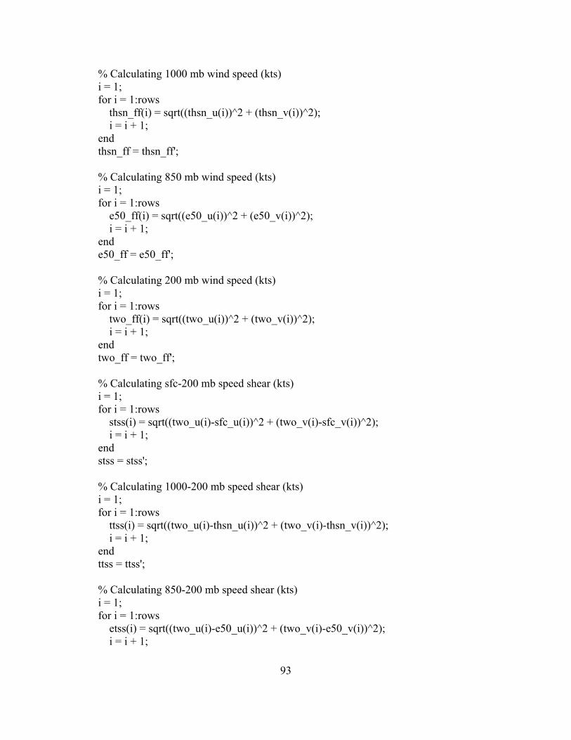
93
% Calculating 1000 mb wind speed (kts) i = 1; for i = 1:rows thsn_ff(i) = sqrt((thsn_u(i))^2 + (thsn_v(i))^2); i = i + 1; end thsn_ff = thsn_ff'; % Calculating 850 mb wind speed (kts) i = 1; for i = 1:rows e50_ff(i) = sqrt((e50_u(i))^2 + (e50_v(i))^2); i = i + 1; end e50_ff = e50_ff'; % Calculating 200 mb wind speed (kts) i = 1; for i = 1:rows two_ff(i) = sqrt((two_u(i))^2 + (two_v(i))^2); i = i + 1; end two_ff = two_ff'; % Calculating sfc-200 mb speed shear (kts) i = 1; for i = 1:rows stss(i) = sqrt((two_u(i)-sfc_u(i))^2 + (two_v(i)-sfc_v(i))^2); i = i + 1; end stss = stss'; % Calculating 1000-200 mb speed shear (kts) i = 1; for i = 1:rows ttss(i) = sqrt((two_u(i)-thsn_u(i))^2 + (two_v(i)-thsn_v(i))^2); i = i + 1; end ttss = ttss'; % Calculating 850-200 mb speed shear (kts) i = 1; for i = 1:rows etss(i) = sqrt((two_u(i)-e50_u(i))^2 + (two_v(i)-e50_v(i))^2); i = i + 1;

94
end etss = etss'; % Calculating sfc wind direction i = 1; for i = 1:rows if sfc_v(i) >= 0 theta = 180; elseif sfc_u(i) < 0 && sfc_v(i) < 0 theta = 0; elseif sfc_u(i) >= 0 && sfc_v(i) < 0 theta = 360; end ddr_sfc(i) = atan(sfc_u(i) / sfc_v(i)); sfc_dd(i) = ((ddr_sfc(i) / 3.1415927) * 180) + theta; if sfc_dd(i) > 360 sfc_dd(i) = sfc_dd(i) - 360; end i = i + 1; end sfc_dd = sfc_dd'; % Calculating 1000 mb wind direction i = 1; for i = 1:rows if thsn_v(i) >= 0 theta = 180; elseif thsn_u(i) < 0 && thsn_v(i) < 0 theta = 0; elseif thsn_u(i) >= 0 && thsn_v(i) < 0 theta = 360; end ddr_thsn(i) = atan(thsn_u(i) / thsn_v(i)); thsn_dd(i) = ((ddr_thsn(i) / 3.1415927) * 180) + theta; if thsn_dd(i) > 360 thsn_dd(i) = thsn_dd(i) - 360; end i = i + 1; end thsn_dd = thsn_dd'; % Calculating 850 mb wind direction i = 1; for i = 1:rows if e50_v(i) >= 0

95
theta = 180; elseif e50_u(i) < 0 && e50_v(i) < 0 theta = 0; elseif e50_u(i) >= 0 && e50_v(i) < 0 theta = 360; end ddr_e50(i) = atan(e50_u(i) / e50_v(i)); e50_dd(i) = ((ddr_e50(i) / 3.1415927) * 180) + theta; if e50_dd(i) > 360 e50_dd(i) = e50_dd(i) - 360; end i = i + 1; end e50_dd = e50_dd'; % Calculating 200 mb wind direction i = 1; for i = 1:rows if two_v(i) >= 0 theta = 180; elseif two_u(i) < 0 && two_v(i) < 0 theta = 0; elseif two_u(i) >= 0 && two_v(i) < 0 theta = 360; end ddr_two(i) = atan(two_u(i) / two_v(i)); two_dd(i) = ((ddr_two(i) / 3.1415927) * 180) + theta; if two_dd(i) > 360 two_dd(i) = two_dd(i) - 360; end i = i + 1; end two_dd = two_dd'; % Calculating sfc-200 mb directional shear i = 1; for i = 1:rows if two_dd(i) > sfc_dd(i) if two_dd(i) - sfc_dd(i) <= 180 stds(i) = two_dd(i) - sfc_dd(i); end if two_dd(i) - sfc_dd(i) > 180 stds(i) = (360 - two_dd(i)) + sfc_dd(i); end end
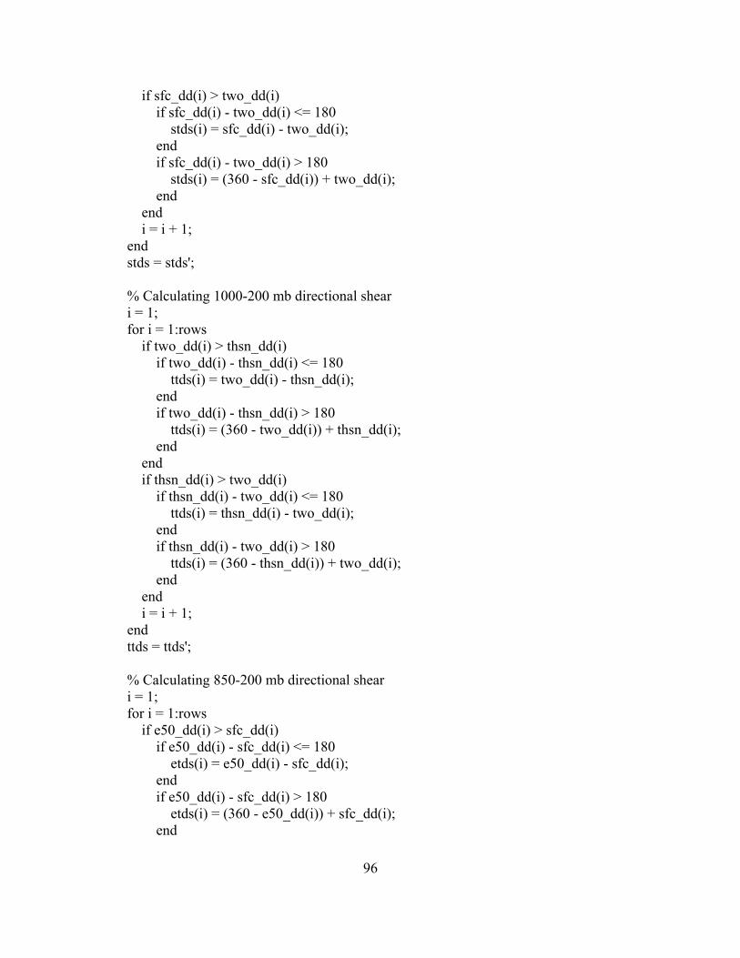
96
if sfc_dd(i) > two_dd(i) if sfc_dd(i) - two_dd(i) <= 180 stds(i) = sfc_dd(i) - two_dd(i); end if sfc_dd(i) - two_dd(i) > 180 stds(i) = (360 - sfc_dd(i)) + two_dd(i); end end i = i + 1; end stds = stds'; % Calculating 1000-200 mb directional shear i = 1; for i = 1:rows if two_dd(i) > thsn_dd(i) if two_dd(i) - thsn_dd(i) <= 180 ttds(i) = two_dd(i) - thsn_dd(i); end if two_dd(i) - thsn_dd(i) > 180 ttds(i) = (360 - two_dd(i)) + thsn_dd(i); end end if thsn_dd(i) > two_dd(i) if thsn_dd(i) - two_dd(i) <= 180 ttds(i) = thsn_dd(i) - two_dd(i); end if thsn_dd(i) - two_dd(i) > 180 ttds(i) = (360 - thsn_dd(i)) + two_dd(i); end end i = i + 1; end ttds = ttds'; % Calculating 850-200 mb directional shear i = 1; for i = 1:rows if e50_dd(i) > sfc_dd(i) if e50_dd(i) - sfc_dd(i) <= 180 etds(i) = e50_dd(i) - sfc_dd(i); end if e50_dd(i) - sfc_dd(i) > 180 etds(i) = (360 - e50_dd(i)) + sfc_dd(i); end

97
end if sfc_dd(i) > e50_dd(i) if sfc_dd(i) - e50_dd(i) <= 180 etds(i) = sfc_dd(i) - e50_dd(i); end if sfc_dd(i) - e50_dd(i) > 180 etds(i) = (360 - sfc_dd(i)) + e50_dd(i); end end i = i + 1; end etds = etds'; % Displaying individual arrays of shear values sfc_u sfc_v sfc_ff sfc_dd thsn_u thsn_v thsn_ff thsn_dd e50_u e50_v e50_ff e50_dd two_u two_v two_ff two_dd stss ttss etss stds ttds etds

98
Appendix C: Complete Set of Splitting Rules
This is the complete listing of splitting rules and number of records per terminal node. The splitting rules are the same regardless of class assignment, and this appendix should be used with Figure 23 to obtain an overall awareness of the classification tree.
Terminal Node Number of Records Splitting Rule 1 61 SFC T < 26.89 & AGE < 13.5 2 13 SFC T < 26.89 & AGE > 13.5 & AGE < 45.5 & LAT < 13 3 13 SFC T < 26.89 & AGE > 13.5 & AGE < 45.5 & LAT > 13 & SST < 18.5 4 108 SFC T < 26.89 & AGE > 13.5 & AGE < 45.5 & LAT > 13 & SST > 18.5 5 2 SFC T < 26.89 & AGE > 45.5 & LAT < 17.35 6 97 SFC T < 26.89 & AGE > 45.5 & LAT > 17.35 7 206 SFC T > 26.89 & E50 T < 18.99 & LAT < 17.7 8 25 SFC T > 26.89 & E50 T < 18.99 & LAT > 17.7 & AGE < 17
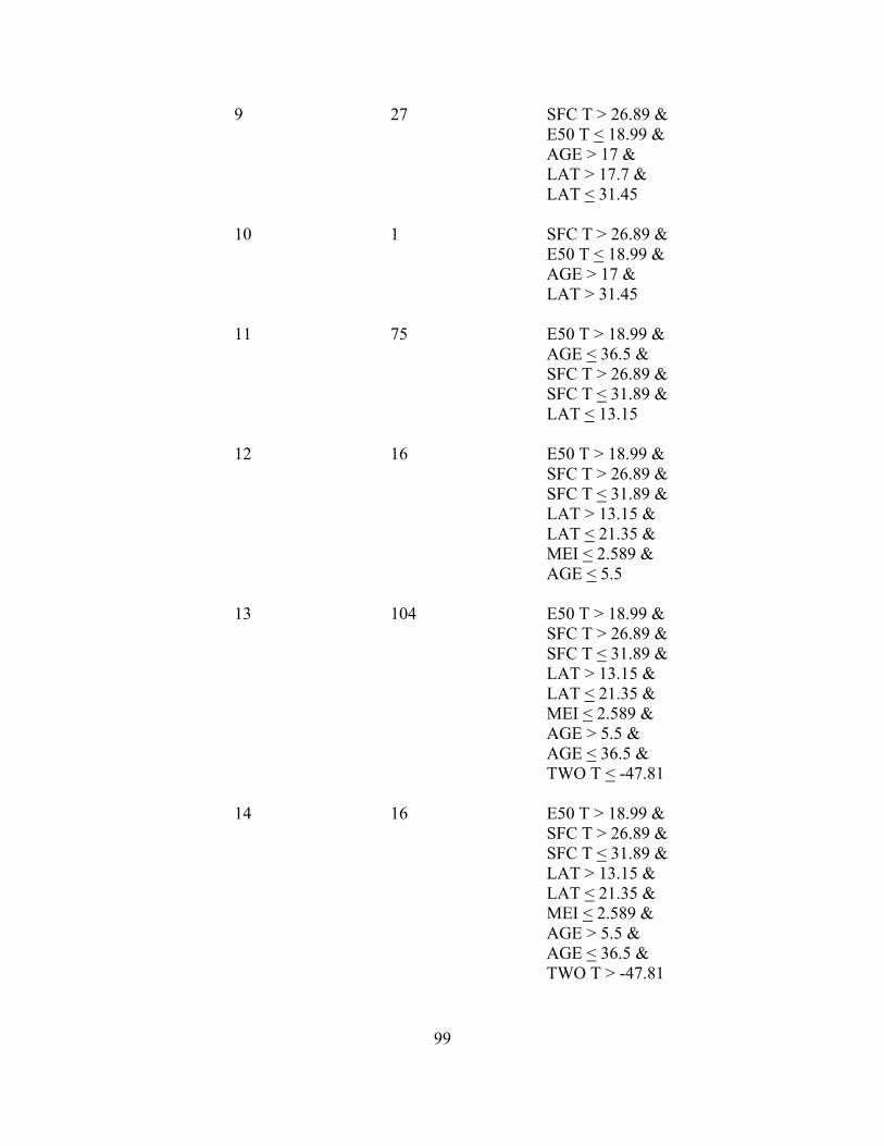
99
9 27 SFC T > 26.89 & E50 T < 18.99 & AGE > 17 & LAT > 17.7 & LAT < 31.45 10 1 SFC T > 26.89 & E50 T < 18.99 & AGE > 17 & LAT > 31.45 11 75 E50 T > 18.99 & AGE < 36.5 & SFC T > 26.89 & SFC T < 31.89 & LAT < 13.15 12 16 E50 T > 18.99 & SFC T > 26.89 & SFC T < 31.89 & LAT > 13.15 & LAT < 21.35 & MEI < 2.589 & AGE < 5.5 13 104 E50 T > 18.99 & SFC T > 26.89 & SFC T < 31.89 & LAT > 13.15 & LAT < 21.35 & MEI < 2.589 & AGE > 5.5 & AGE < 36.5 & TWO T < -47.81 14 16 E50 T > 18.99 & SFC T > 26.89 & SFC T < 31.89 & LAT > 13.15 & LAT < 21.35 & MEI < 2.589 & AGE > 5.5 & AGE < 36.5 & TWO T > -47.81
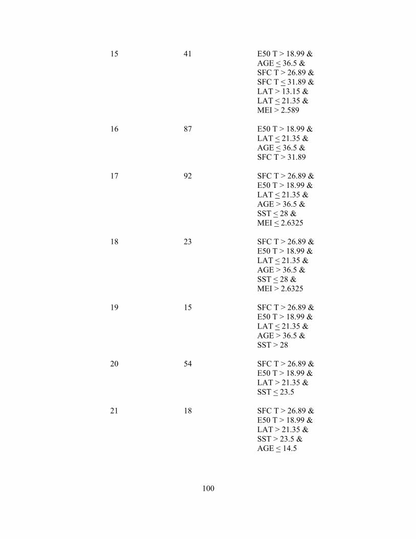
100
15 41 E50 T > 18.99 & AGE < 36.5 & SFC T > 26.89 & SFC T < 31.89 & LAT > 13.15 & LAT < 21.35 & MEI > 2.589 16 87 E50 T > 18.99 & LAT < 21.35 & AGE < 36.5 & SFC T > 31.89 17 92 SFC T > 26.89 & E50 T > 18.99 & LAT < 21.35 & AGE > 36.5 & SST < 28 & MEI < 2.6325 18 23 SFC T > 26.89 & E50 T > 18.99 & LAT < 21.35 & AGE > 36.5 & SST < 28 & MEI > 2.6325 19 15 SFC T > 26.89 & E50 T > 18.99 & LAT < 21.35 & AGE > 36.5 & SST > 28 20 54 SFC T > 26.89 & E50 T > 18.99 & LAT > 21.35 & SST < 23.5 21 18 SFC T > 26.89 & E50 T > 18.99 & LAT > 21.35 & SST > 23.5 & AGE < 14.5
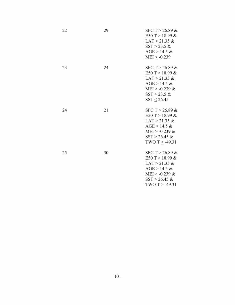
101
22 29 SFC T > 26.89 & E50 T > 18.99 & LAT > 21.35 & SST > 23.5 & AGE > 14.5 & MEI < -0.239 23 24 SFC T > 26.89 & E50 T > 18.99 & LAT > 21.35 & AGE > 14.5 & MEI > -0.239 & SST > 23.5 & SST < 26.45 24 21 SFC T > 26.89 & E50 T > 18.99 & LAT > 21.35 & AGE > 14.5 & MEI > -0.239 & SST > 26.45 & TWO T < -49.31 25 30 SFC T > 26.89 & E50 T > 18.99 & LAT > 21.35 & AGE > 14.5 & MEI > -0.239 & SST > 26.45 & TWO T > -49.31

102
Acronyms
AFCCC Air Force Combat Climatology Center AFWA Air Force Weather Agency AMS American Meteorological Society ATCF Automated Tropical Cyclone Forecasting BF Banding Features BOM Bureau of Meteorology BT Best Track CART Classification and Regression Tree CAT Categorical Cb Cumulonimbus CDO Central Dense Overcast CF Central Features CI Current Intensity CPC Climate Prediction Center Cu Cumulus D Double Channel Outflow EN El Niño FGGE First GARP Global Experiment FLENUMMETOC Fleet Numerical Meteorology and Oceanography FSR Forecast Splitting Rules GPH Geopotential Height GTCCA Global Tropical Cyclone Climatic Atlas IPV Isentropic Potential Vorticity JTWC Joint Typhoon Warning Center LN La Niña MEI Multivariate ENSO Index MPI Maximum Potential Intensity MSE Mean Squared Error MSLP Minimum Sea Level Pressure MSWT Major Shortwave Trough MWS Maximum Wind Speed N No Channel Outflow NCDC National Climatic Data Center NCEP National Centers for Environmental Prediction NH Northern Hemisphere NOGAPS Navy Operational Global Atmospheric Prediction System NRL Naval Research Laboratory NU Neutral PV Potential Vorticity PVMAX Potential Vorticity Maximum PVU Potential Vorticity Unit

103
RC Relative Cost RH Relative Humidity RMSE Root Mean Squared Error S Single Channel Outflow SE Single Channel Outflow (Equatorward) SP Single Channel Outflow (Poleward) SAFA Systematic Approach to Tropical Cyclone Forecasting Aid SFCTMP Surface Temperature SH Southern Hemisphere SOI Southern Oscillation Index SST Sea Surface Temperature TC Tropical Cyclone TD Tropical Depression TS Tropical Storm TUTT Tropical Upper Tropospheric Trough UC Upper Cyclone UTC Coordinated Universal Time UTFT Upper Tropospheric Flow Transitions WISHE Wind Induced Surface Heat Exchange

104
Bibliography
Benz, R.F. Data Mining Atmospheric/Oceanic Parameters in the Design of a Long-Range Nephelometric Forecast Tool. MS Thesis, AFIT/GM/03-02. School of Engineering Physics, Air Force Institute of Technology (AU), Wright-Patterson AFB OH, March 2003 (ADA412870).
Black, P.G. and Shay, L.K., 1998: Air-sea interaction processes relevant to tropical
cyclone intensity change. Special Sessions on Tropical Cyclone Intensity Change, AMS 78th Annual Meeting, Phoenix, AZ, 11-16 Jan, 1998.
Bluestein, H.B., 1993: Synoptic-Dynamic Meteorology in Midlatitudes, Volume II.
Oxford University Press, 594 pp. Bosart, L.F., Velden, C.S., Bracken, W.E., Molinari, J. and Black P.G., 2000:
Environmental influences on the rapid intensification of Hurricane Opal (1995) over the Gulf of Mexico, Monthly Weather Review, 128, 322-352.
Breiman, L., Friedman, J.H., Olshen, R.A. and Stone, C.J., 1984: Classification and
Regression Trees. Wadsworth, Belmont, CA, 358 pp. Chen, L. and Gray, W.M., 1985: Global view of the upper level outflow patterns
associated with tropical cyclone intensity changes during FGGE, Dept. of Atmos. Sci., Paper No. 392, Colorado State University, Ft. Collins, CO, 118 pp.
D’Aleo, J.S. and Grube, P.G., 2002: The Oryx Resource Guide to El Niño and La Niña.
Oryx Press, 230 pp. Davidson, N.E. and Kar, S.K., 2002: Upper-tropospheric flow transitions during rapid
tropical cyclone intensification, Quarterly Journal of the Royal Meteorological Society, 128, 861-891.
DeMaria, M., 1996: The effect of vertical shear on tropical cyclone intensity change,
Journal of the Atmospheric Sciences, 53, 2076-2087. Dvorak, V.F., 1974: Tropical cyclone intensity analysis and forecasting from satellite
imagery, Monthly Weather Review, 103, 420-430. Emanuel, K.A., 1986: An air-sea interaction theory for tropical cyclones. Part I: Steady-
state maintenance, Journal of the Atmospheric Sciences, 43, 585-604. Evans, J.L., 1993: Sensitivity of tropical cyclone intensity to sea surface temperature,
Journal of Climate, 6, 1133-1140.

105
Ferreira, R.N. and Schubert, W.H., 1999: The role of tropical cyclones in the formation of tropical upper-tropospheric troughs, Journal of the Atmospheric Sciences, 56, 2891-2584.
Ford, B.W. El Nino and La Nina Effects on Tropical Cyclones: The Mechanisms. MS
Thesis. Naval Postgraduate School (NPS), Monterey CA, June 2000 (ADA380280).
Glickman, T.S., 2000: Glossary of Meteorology. American Meteorological Society, 855
pp. Global Tropical Cyclone Climatic Atlas, 2003: Tropical Cyclone Tracks 1997, 1999, and
2001 [Online at http://navy.ncdc.noaa.gov/products/gtcca/gtccamain.html]. Goerss, J.S. and Jeffries, R.A., 1994: Assimilation of synthetic tropical cyclone
observations into the navy operational global atmospheric prediction system, Weather and Forecasting, 9, 557-576.
Hanley, D., Molinari, J. and Keyser, D., 2001: A composite study of the interactions
between tropical cyclones and upper-tropospheric troughs, Monthly Weather Review, 129, 2570-2584.
Holland, G.J., 1997: The maximum potential intensity of tropical cyclones, Journal of the
Atmospheric Sciences, 54, 2519-2541. Holliday, C.R. and Thompson, A.H., 1979: Climatological characteristics of rapidly
intensifying typhoons, Monthly Weather Review, 107, 1022-1034. Hoskins, B.J., McIntyre, M.E. and Robertson, A.W., 1985: On the use and significance of
isentropic potential vorticity maps, Quarterly Journal of the Royal Meteorological Society, 111, 877-946.
Joint Typhoon Warning Center (JTWC) Website, 2003: TDO Handbook [Online at
https://pzal.npmoc.navy.mil/training/tdohandbook/TOC.htm]. Joint Typhoon Warning Center (JTWC) Website, 2003: TC Intensity Analysis Worksheet
[Online at https://pzal.npmoc.navy.mil/training/research/ TCIntens.html]. Kelley, W.E., Jr. and Mock, D.R., 1982: A diagnostic study of upper tropospheric cold
lows over the western North Pacific, Monthly Weather Review, 110, 471-480. Kopp, T.J., 1995: The Air Force Global Weather Central Surface Temperature Model,
Air Force Global Weather Central Technical Note 95/004, 23 pp.

106
McNamara, T., 2001. The Dvorak Technique for tropical cyclone analysis. Advanced Synoptic Meteorology PowerPoint Presentation. Department of Engineering Physics, Air Force Institute of Technology, Wright-Patterson AFB, OH.
Merrill, R.T., 1987: An experiment in the statistical prediction of tropical cyclone
intensity change. NOAA Technical Memorandum, NWS, NHC 34, 33 pp. Merrill, R.T., 1988: Environmental influences on hurricane intensification, Journal of the
Atmospheric Sciences, 45, 1678-1687. Molinari, J., Skubis, S., Vollaro, D. and Alsheimer, F., 1998: Potential vorticity analysis
of tropical cyclone intensification, Journal of the Atmospheric Sciences, 55, 2632-2644.
Montgomery, D.C. and Runger, G.C., 2002: Applied Statistics and Probability for
Engineers, 3rd Edition. John Wiley and Sons, Inc., 720 pp. Naval Research Laboratory (NRL) Website, 1998: TC Forecaster’s Reference Guide [Online at http://www.nrlmry.navy.mil/~chu/tropcycl.htm]. Nyoumura, Y. and Yamashita, H., 1984: On the central pressure change of tropical
cyclones as a function of sea surface temperature and land effect, Geophysical Magazine, 41, 45-59.
Price, J.D. and Vaughan, G., 1992: Statistical studies of cut-off-low systems, Annales
Geophysicae, 10, 96-102. Randall, R.M. Exploration of Teleconnection Indices for Long-Range Seasonal
Temperature Forecasts. MS Thesis, AFIT/GM/02-08. School of Engineering Physics, Air Force Institute of Technology (AU), Wright-Patterson AFB OH, March 2002 (ADA404188).
Sadler, J.C., 1964: Tropical cyclones of the Eastern North Pacific as revealed by TIROS
observations, Journal of Applied Meteorology, 3, 347-366. Sadler, J.C., 1975: The upper tropospheric circulation over the global tropics, Dept. of
Meteorology, University of Hawaii, Rep. UHMET 75-05, 35 pp. Sadler, J.C., 1978: Mid-season typhoon development and intensity changes and the
tropical upper tropospheric trough, Monthly Weather Review, 106, 1137-1152. Salford Systems, 1995: Data Mining with Decision Trees: An Introduction to CART®.
San Diego, CA, 133 pp. Salford Systems, 2002: CART® for Windows User’s Guide. San Diego, CA, 295 pp.

107
Sikora, C.R., 1976: An investigation of equivalent potential temperature as a measure of tropical cyclone intensity, FLEWEACEN Technical Note JTWC 76-3, 12 pp.
Steinberg, D. and Colla, P., 1995: CART: Tree-structured nonparametric data analysis.
San Diego, CA: Salford Systems, 355 pp. Thorpe, A. J., 1986: Synoptic-scale disturbances with circular symmetry, Monthly
Weather Review, 114, 1384-1389. University Center for Atmospheric Research (UCAR) Website, 2004: NOGAPS 4.0 [Online at http://meted.ucar.edu/nwp/pcu2/nogaps]. Vilpors, S. Techniques Development Officer, Joint Typhoon Warning Center, Hickam
AB, Hawaii. Personal Correspondences. February - December 2003. Whitfield, M.B. and Lyons, S.W., 1992: An upper-level low over Texas during summer,
Weather and Forecasting, 7, 89-106. Wilks, D.S., 1995: Statistical Methods in the Atmospheric Sciences. Academic Press,
467 pp.

108
Vita
Capt Jonathan Leffler was born in Phoenix, Arizona. He graduated from Canon
City High School and graduated from the University of Northern Colorado with a
Bachelor of Science degree in Meteorology. In 1997, he entered active duty after
attending Officer Training School at Maxwell AFB, Alabama.
His first assignment was Wing Weather Officer for the 28th Operational Support
Squadron, Ellsworth AFB, South Dakota. In 1999, Capt Leffler was assigned as
Assistant Flight Commander, A-Flight, to the USAFE Operational Weather Squadron,
Sembach AB, Germany. In 2001, he became Flight Commander of A-Flight. While
serving in Germany, Capt Leffler qualified for Foreign Area Officer and attended the
French Language and Area Studies Immersion Program in Nice, France. He was also
selected to attend the Air Force Institute of Technology in 2002. Capt Leffler is married
and has one daughter.

109
REPORT DOCUMENTATION PAGE Form Approved OMB No. 074-0188
The public reporting burden for this collection of information is estimated to average 1 hour per response, including the time for reviewing instructions, searching existing data sources, gathering and maintaining the data needed, and completing and reviewing the collection of information. Send comments regarding this burden estimate or any other aspect of the collection of information, including suggestions for reducing this burden to Department of Defense, Washington Headquarters Services, Directorate for Information Operations and Reports (0704-0188), 1215 Jefferson Davis Highway, Suite 1204, Arlington, VA 22202-4302. Respondents should be aware that notwithstanding any other provision of law, no person shall be subject to an penalty for failing to comply with a collection of information if it does not display a currently valid OMB control number. PLEASE DO NOT RETURN YOUR FORM TO THE ABOVE ADDRESS. 1. REPORT DATE (DD-MM-YYYY) March 2004
2. REPORT TYPE Master’s Thesis
3. DATES COVERED (From – To) Jun 2003 – Mar 2004
5a. CONTRACT NUMBER
5b. GRANT NUMBER
4. TITLE AND SUBTITLE FEASIBILITY OF USING CLASSIFICATION ANALYSES TO DETERMINE TROPICAL CYCLONE RAPID INTENSIFICATION
5c. PROGRAM ELEMENT NUMBER
5d. PROJECT NUMBER 5e. TASK NUMBER
6. AUTHOR(S) Leffler, Jonathan W., Captain, USAF 5f. WORK UNIT NUMBER
7. PERFORMING ORGANIZATION NAMES(S) AND ADDRESS(S) Air Force Institute of Technology Graduate School of Engineering and Management (AFIT/ENP) 2950 Hobson Way, Bldg 640 WPAFB OH 45433-7765
8. PERFORMING ORGANIZATION REPORT NUMBER AFIT/GM/ENP/04-07
10. SPONSOR/MONITOR’S ACRONYM(S)
9. SPONSORING/MONITORING AGENCY NAME(S) AND ADDRESS(ES) Naval Pacific Meteorology and Oceanography Center/Joint Typhoon Warning Center 425 Luapele Road Pearl Harbor, HI 96860-3103
11. SPONSOR/MONITOR’S REPORT NUMBER(S)
12. DISTRIBUTION/AVAILABILITY STATEMENT APPROVED FOR PUBLIC RELEASE; DISTRIBUTION UNLIMITED. 13. SUPPLEMENTARY NOTES 14. ABSTRACT Tropical cyclone intensity techniques developed by Dvorak have thus far been regarded by tropical meteorologists as the best identification and forecast schemes available using satellite imagery. However, in recent years, several ideologies have arisen which discuss alternative means of determining typhoon rapid intensification or weakening in the Pacific. These theories include examining channel outflow patterns, potential vorticity superposition and anomalies, tropical upper tropospheric trough interactions, environmental influences, and upper tropospheric flow transitions. It is now possible to data mine these atmospheric parameters thought partly responsible for typhoon rapid intensification and weakening to validate their usefulness in the forecast process. Using the latest data mining software tools, this study used components of NOGAPS analyses along with selected atmospheric and climatological predictors in classification analyses to create conditional forecast decision trees. The results of the classification model show an approximate R2 of 0.68 with percent error misclassifications of 13.5% for rapidly weakening typhoon events and 21.8% for rapidly intensifying typhoon events. In addition, a merged set of suggested forecast splitting rules was developed. By using the three most accurate predictors from both intensifying and weakening storms, the results validate the notion that multiple parameters are responsible for rapid changes in typhoon development. 15. SUBJECT TERMS Classification and Regression Tree, CART, Tropical Cyclone Intensification, Typhoon Intensification
16. SECURITY CLASSIFICATION OF: 19a. NAME OF RESPONSIBLE PERSON Lt Col Ronald P. Lowther, ENP
a. REPORT
U
b. ABSTRACT
U
c. THIS PAGE U
17. LIMITATION OF ABSTRACT UU
18. NUMBER OF PAGES 121
19b. TELEPHONE NUMBER (Include area code) (937) 255-3636, ext 4645
Standard Form 298 (Rev. 8-98) Prescribed by ANSI Std. Z39-18