Embed Size (px)
Citation preview
Umesh Gauli
Feasibility Study on a Large Scale Solar PV System
Helsinki Metropolia University of Applied Sciences
Bachelor of Engineering
Environmental Engineering
Bachelor´s Thesis
28 April 2016
Abstract
Author(s) Title Number of Pages Date
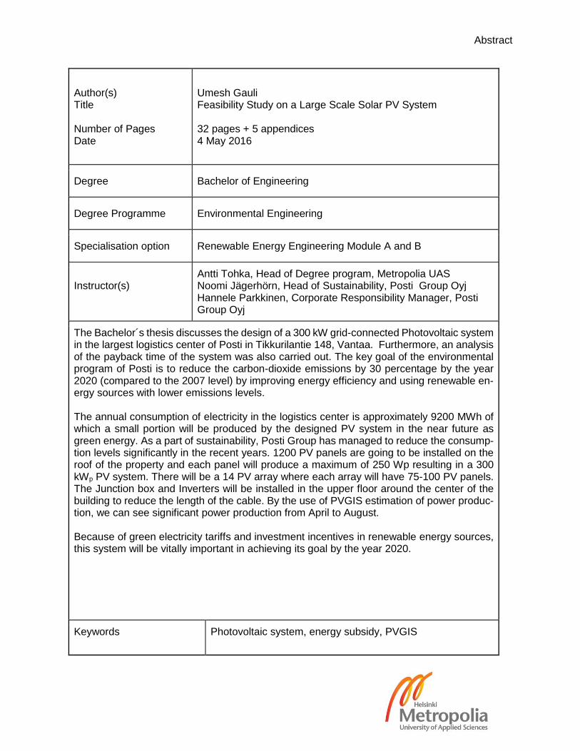
Umesh Gauli Feasibility Study on a Large Scale Solar PV System 32 pages + 5 appendices 4 May 2016
Degree Bachelor of Engineering
Degree Programme Environmental Engineering
Specialisation option Renewable Energy Engineering Module A and B
Instructor(s)
Antti Tohka, Head of Degree program, Metropolia UAS Noomi Jägerhörn, Head of Sustainability, Posti Group Oyj Hannele Parkkinen, Corporate Responsibility Manager, Posti Group Oyj
The Bachelor´s thesis discusses the design of a 300 kW grid-connected Photovoltaic system in the largest logistics center of Posti in Tikkurilantie 148, Vantaa. Furthermore, an analysis of the payback time of the system was also carried out. The key goal of the environmental program of Posti is to reduce the carbon-dioxide emissions by 30 percentage by the year 2020 (compared to the 2007 level) by improving energy efficiency and using renewable en-ergy sources with lower emissions levels. The annual consumption of electricity in the logistics center is approximately 9200 MWh of which a small portion will be produced by the designed PV system in the near future as green energy. As a part of sustainability, Posti Group has managed to reduce the consump-tion levels significantly in the recent years. 1200 PV panels are going to be installed on the roof of the property and each panel will produce a maximum of 250 Wp resulting in a 300 kWp PV system. There will be a 14 PV array where each array will have 75-100 PV panels. The Junction box and Inverters will be installed in the upper floor around the center of the building to reduce the length of the cable. By the use of PVGIS estimation of power produc-tion, we can see significant power production from April to August. Because of green electricity tariffs and investment incentives in renewable energy sources, this system will be vitally important in achieving its goal by the year 2020.
Keywords Photovoltaic system, energy subsidy, PVGIS
2
Table of Contents
1 Introduction 7
2 Methodology 7
3 Description of the site 7
3.1 Consumption data of 2015 9
3.2 Consumption in summer and winter day 11
4 The Solar PV System 12
4.1 Major system Component 13
4.2 PV Energy potential in Europe and Finland 13
4.3 Energy Losses in PV System 16
4.3.1 Pre-module Losses 16
4.3.2 Module losses 16
4.3.3 System Losses 16
5 Design Parameters 17
5.1 Selection and sizing of PV-Panels 17
5.2 Azimuth 19
5.3 Inclination 19
5.4 Array Spacing 19
5.5 Temperature co-efficient 21
5.6 Inverter selection and manufacture type 22
5.6.1 Features of ABB Pro 33 inverter 22
6 Output Power 23
6.1 Power production on a summer day 25
6.2 Production Vs Demand 25
7 Payback time 26
7.1 Uncertainty of the investment 28
7.2 Return of investment (ROI) 28
7.3 Price of electricity 28
3
7.4 Feasibility study 29
8 Conclusions 30
References 31
9 Appendices 33
9.1 Electricity consumption in summer day and winter day 33
9.2 Global irradiation and PV potential in Europe 34
9.3 Pre-sizing of the system using PVSYST software 35
9.4 Saana 245-255 TP3 MBW specification 36
4
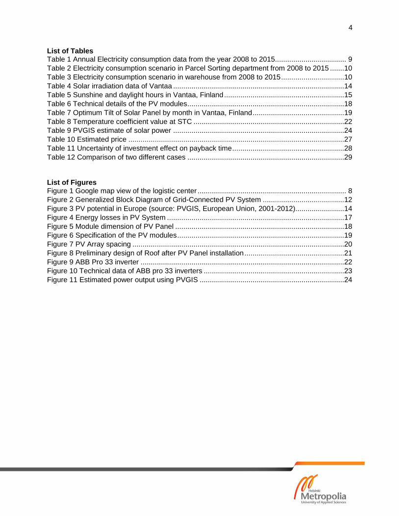
List of Tables Table 1 Annual Electricity consumption data from the year 2008 to 2015................................... 9
Table 2 Electricity consumption scenario in Parcel Sorting department from 2008 to 2015 .......10
Table 3 Electricity consumption scenario in warehouse from 2008 to 2015 ...............................10
Table 4 Solar irradiation data of Vantaa ....................................................................................14
Table 5 Sunshine and daylight hours in Vantaa, Finland ...........................................................15
Table 6 Technical details of the PV modules .............................................................................18
Table 7 Optimum Tilt of Solar Panel by month in Vantaa, Finland .............................................19
Table 8 Temperature coefficient value at STC ..........................................................................22
Table 9 PVGIS estimate of solar power ....................................................................................24
Table 10 Estimated price ..........................................................................................................27
Table 11 Uncertainty of investment effect on payback time .......................................................28
Table 12 Comparison of two different cases .............................................................................29
List of Figures Figure 1 Google map view of the logistic center ......................................................................... 8
Figure 2 Generalized Block Diagram of Grid-Connected PV System ........................................12
Figure 3 PV potential in Europe (source: PVGIS, European Union, 2001-2012) ........................14
Figure 4 Energy losses in PV System .......................................................................................17
Figure 5 Module dimension of PV Panel ...................................................................................18
Figure 6 Specification of the PV modules ..................................................................................19
Figure 7 PV Array spacing ........................................................................................................20
Figure 8 Preliminary design of Roof after PV Panel installation .................................................21
Figure 9 ABB Pro 33 inverter ....................................................................................................22
Figure 10 Technical data of ABB pro 33 inverters .....................................................................23
Figure 11 Estimated power output using PVGIS .......................................................................24

5
Acknowledgement
I would like to take this opportunity to express my gratitude to all those persons who have given their valuable instructions, support, and assistance. Firstly, I wish to express my sincere thanks to my thesis supervisor Mr. Antti Tohka for his guidelines and supervision. Secondly, I would like thank Noomi Jägerhörn and Hannele Parkkinen from Posti Group Oyj. And I take this opportunity to record my sincere thanks and deepest gratitude to all those who have directly and indirectly guided me. Lastly, my special thanks to my family and all the staff of Metropolia UAS.
6
Abbreviations
kWh kilowatt-hour kW kilowatt PV photovoltaic DC Direct Current AC Alternating Current BOS Balance of system equipment PR Performance Ratio EU European Union STC Standard Test Condition W Watt ROI Return of investment
7
1 Introduction
Finland is one of the leading users of renewable sources of energy in the world. About 1/4th of the total energy consumption in Finland is provided by renewable energy sources. Bio-energy, wood-based fuels, wind energy, geothermal heat and solar energy are the most common sources of renewable energy. The key goal of the environmental program of Posti Group is to reduce the carbon dioxide emis-sions by 30 percentage by the year 2020 (compared to the 2007 level) by improving energy effi-ciency and using renewable energy sources with lower emissions levels. Posti has managed to reduce the electrical consumption by 3 % and heating consumption by 17%. Temperature adjusted heat consumption has been decreased by 9 %. Generally, 80 % of the consumed electricity is used in large properties such as parcel sorting, warehouse, and postal center. The plan is to design a grid connected to the solar PV system which supplies the electricity for one of the largest logistics centers of Posti located in Vantaa. This kind of a grid connected system has been popular nowadays because of governmental tariff prices and investment incentives. There has been a significant decrease in the consumption of the electricity as the production facilities of the logistics center have been decreased by one degree Celsius by improving the capturing of exhaust air and updating the timing of lights.
2 Methodology
Following steps were used for the design:-
The power consumption demand of the logistics centre was collected and analysed.
The size and choice of electronic equipment like inverter, cable etc. were determined.
The size of PV module was chosen.
The size and length of cable were decided in order to minimize the loss.
Engineering design: - The optimum angle and azimuthal angle were taken into account when designing PV Array in order to get maximum power output from the system.
3 Description of the site
The logistics center is located in Tikkurilantie 148 which is quite close to Helsinki-Vantaa Interna-tional airport. The latitude of the site is 60018’6” North and the longitude is 24055’30” East and 45 meters above the sea level. The total area of the whole property is 91,965 square kilometers, of which 28,536 square kilometers belong to the Parcel sorting terminal and 63,429 square kilome-ters account for the Warehouse terminal 1-5. The PV panels will be kept on the roof surface of the logistics center. The total area of the roof is approximately 80,000 square kilometers. There are not any obstacles which could make a shadow to the panels mounted on the rooftop of the property.
8
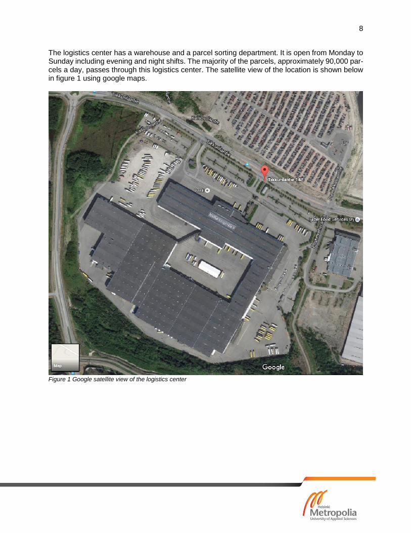
The logistics center has a warehouse and a parcel sorting department. It is open from Monday to Sunday including evening and night shifts. The majority of the parcels, approximately 90,000 par-cels a day, passes through this logistics center. The satellite view of the location is shown below in figure 1 using google maps.
Figure 1 Google satellite view of the logistics center
9
3.1 Consumption data of 2015
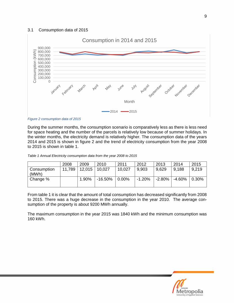
Figure 2 consumption data of 2015
During the summer months, the consumption scenario is comparatively less as there is less need for space heating and the number of the parcels is relatively low because of summer holidays. In the winter months, the electricity demand is relatively higher. The consumption data of the years 2014 and 2015 is shown in figure 2 and the trend of electricity consumption from the year 2008 to 2015 is shown in table 1. Table 1 Annual Electricity consumption data from the year 2008 to 2015
2008 2009 2010 2011 2012 2013 2014 2015
Consumption (MWh)
11,789 12,015 10,027 10,027 9,903 9,629
9,188
9,219
Change %
1.90%
-16.50%
0.00%
-1.20%
-2.80%
-4.60%
0.30%
From table 1 it is clear that the amount of total consumption has decreased significantly from 2008 to 2015. There was a huge decrease in the consumption in the year 2010. The average con-sumption of the property is about 9200 MWh annually. The maximum consumption in the year 2015 was 1840 kWh and the minimum consumption was 160 kWh.
0100,000200,000300,000400,000500,000600,000700,000800,000900,000
Consum
ption (
kW
h)
Month
Consumption in 2014 and 2015
2014 2015
10
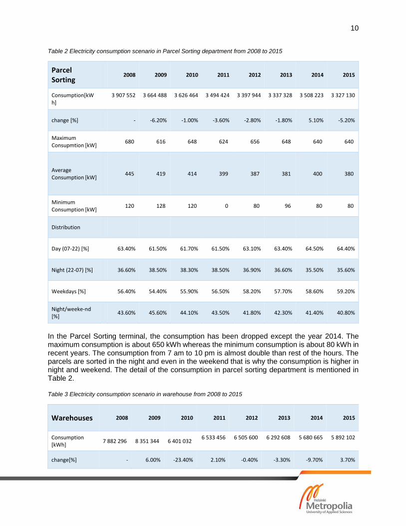
Table 2 Electricity consumption scenario in Parcel Sorting department from 2008 to 2015
Parcel Sorting
2008 2009 2010 2011 2012 2013 2014 2015
Consumption[kWh]
3 907 552
3 664 488
3 626 464
3 494 424
3 397 944
3 337 328
3 508 223
3 327 130
change [%]
- -6.20% -1.00% -3.60% -2.80% -1.80% 5.10% -5.20%
Maximum Consupmtion [kW]
680 616 648 624 656 648 640 640
Average Consumption [kW]
445 419 414 399 387 381 400 380
Minimum Consumption [kW]
120 128 120 0 80 96 80 80
Distribution
Day (07-22) [%]
63.40% 61.50% 61.70% 61.50% 63.10% 63.40% 64.50% 64.40%
Night (22-07) [%]
36.60% 38.50% 38.30% 38.50% 36.90% 36.60% 35.50% 35.60%
Weekdays [%]
56.40% 54.40% 55.90% 56.50% 58.20% 57.70% 58.60% 59.20%
Night/weeke-nd [%]
43.60% 45.60% 44.10% 43.50% 41.80% 42.30% 41.40% 40.80%
In the Parcel Sorting terminal, the consumption has been dropped except the year 2014. The maximum consumption is about 650 kWh whereas the minimum consumption is about 80 kWh in recent years. The consumption from 7 am to 10 pm is almost double than rest of the hours. The parcels are sorted in the night and even in the weekend that is why the consumption is higher in night and weekend. The detail of the consumption in parcel sorting department is mentioned in Table 2. Table 3 Electricity consumption scenario in warehouse from 2008 to 2015
Warehouses 2008 2009 2010 2011 2012 2013 2014 2015
Consumption [kWh]
7 882 296 8 351 344 6 401 032 6 533 456
6 505 600
6 292 608
5 680 665
5 892 102
change[%] - 6.00% -23.40% 2.10% -0.40% -3.30% -9.70% 3.70%
11
Maximum Consumption[kW]
1 312 1 288 1 344 1 336 1 320 1 296 1 200 1 200
Average Consumption[kW]
897 954 731 746 741 718 648 673
Minimum consuption [kW]
208 160 160 0 112 96 80 80
Distribution
Day(07-22) [%] 68.10% 66.10% 72.80% 74.00% 72.30% 74.10% 74.00% 72.00%
Night (22-07) [%] 31.90% 33.90% 27.20% 26.00% 27.70% 25.90% 26.00% 28.00%
Weekdays [%] 61.00% 58.30% 68.80% 70.50% 69.50% 69.90% 69.60% 68.40%
Night/ weekend[%]
39.00% 41.70% 31.20% 29.50% 30.50% 30.10% 30.40% 31.60%
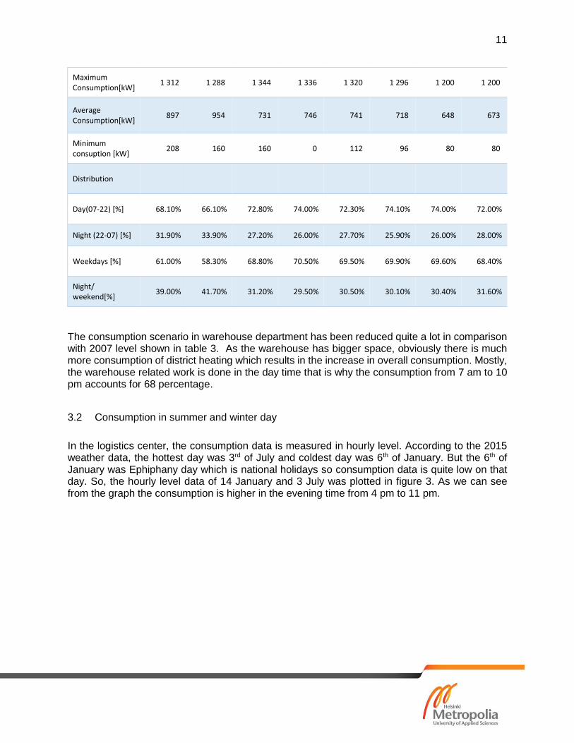
The consumption scenario in warehouse department has been reduced quite a lot in comparison with 2007 level shown in table 3. As the warehouse has bigger space, obviously there is much more consumption of district heating which results in the increase in overall consumption. Mostly, the warehouse related work is done in the day time that is why the consumption from 7 am to 10 pm accounts for 68 percentage.
3.2 Consumption in summer and winter day
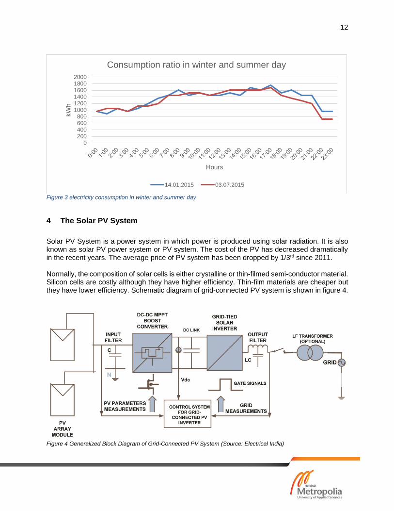
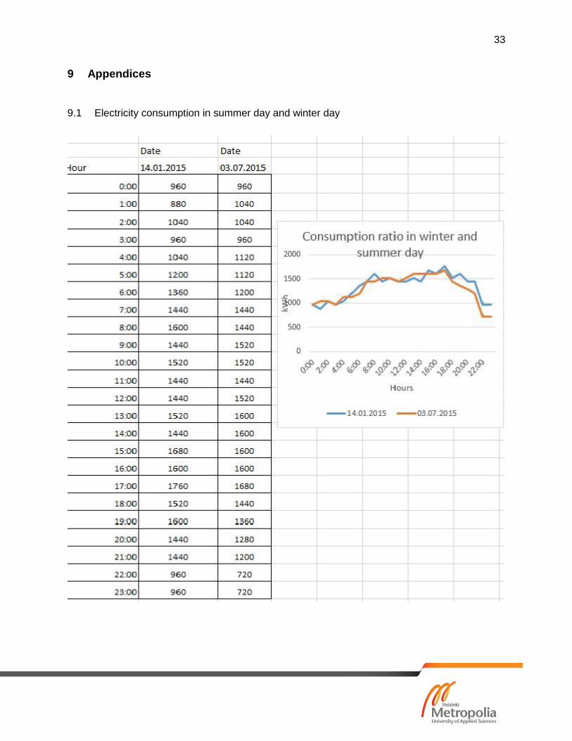
In the logistics center, the consumption data is measured in hourly level. According to the 2015 weather data, the hottest day was 3rd of July and coldest day was 6th of January. But the 6th of January was Ephiphany day which is national holidays so consumption data is quite low on that day. So, the hourly level data of 14 January and 3 July was plotted in figure 3. As we can see from the graph the consumption is higher in the evening time from 4 pm to 11 pm.
12
Figure 3 electricity consumption in winter and summer day
4 The Solar PV System
Solar PV System is a power system in which power is produced using solar radiation. It is also known as solar PV power system or PV system. The cost of the PV has decreased dramatically in the recent years. The average price of PV system has been dropped by 1/3rd since 2011. Normally, the composition of solar cells is either crystalline or thin-filmed semi-conductor material. Silicon cells are costly although they have higher efficiency. Thin-film materials are cheaper but they have lower efficiency. Schematic diagram of grid-connected PV system is shown in figure 4.
Figure 4 Generalized Block Diagram of Grid-Connected PV System (Source: Electrical India)
0200400600800
100012001400160018002000
kW
h
Hours
Consumption ratio in winter and summer day
14.01.2015 03.07.2015
13
4.1 Major system Component
Solar PV system includes various components and they are chosen depending on the site loca-tion, system type, and applications. The major component of the system includes PV panels, junction box, inverter, battery banks and loads.
PV Array- It is made up of PV modules and they are an environmentally-sealed collec-
tion of PV cells which convert sunlight to useful energy. The most common PV cell size
vary from 0.5 to 2.5 square meter. Normally bigger PV cells are used for the bigger sys-
tem.
The Balance of system equipment (BOS) - It includes mounting system and wiring sys-
tem. Ground-fault protection is also included in the wiring system. It is responsible for the
regulating the voltage and current coming from PV Panels and helps battery from over-
charging and prolongs battery life.
Inverter- DC power coming from PV array is changed to standard AC by the inverter.
Metering- It is used to provide an indication of system performance.
Other components- Utility switch
4.2 PV Energy potential in Europe and Finland
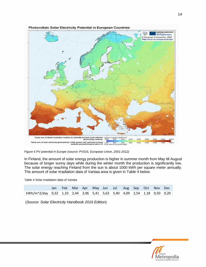
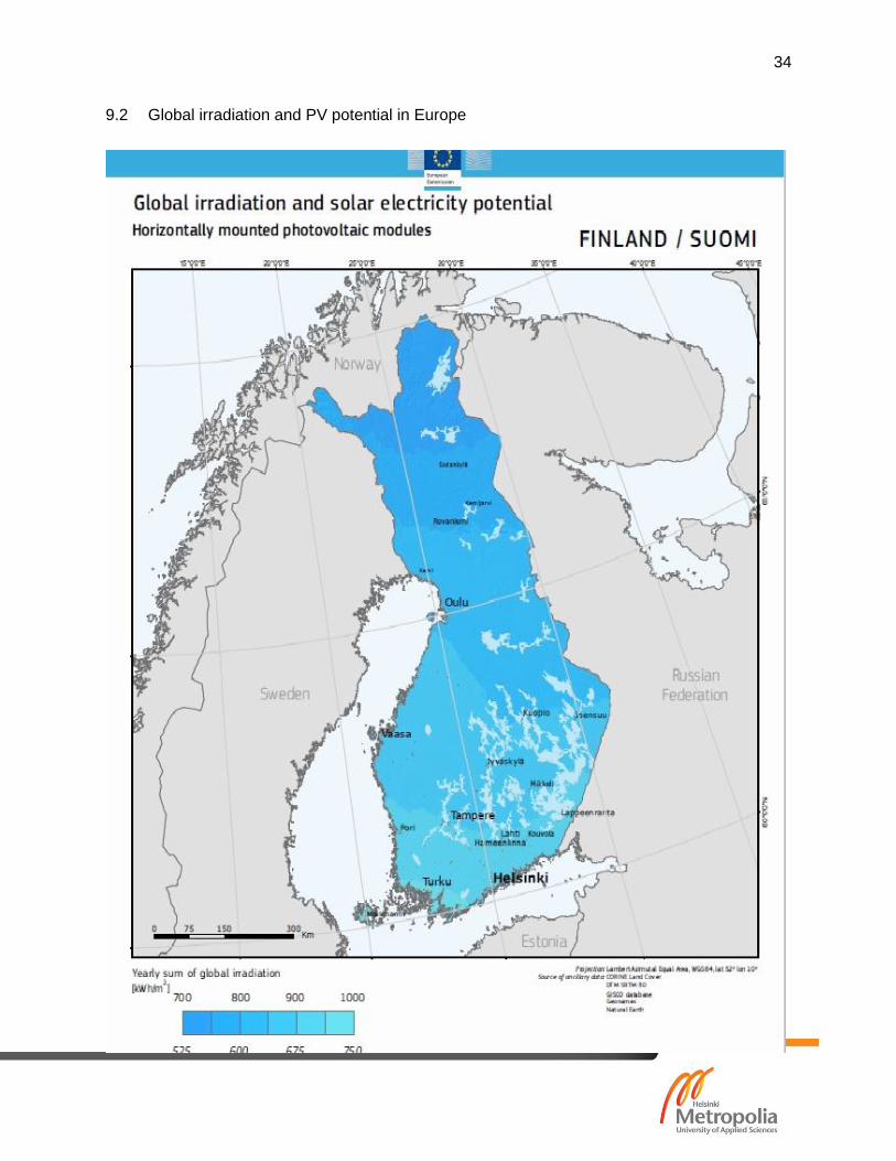
Germany is world’s superpower country in the context of solar energy production. According to 2011 data solar energy production (32,411 MWp) was around 3 % of total energy consumption. From the picture below it is clear that southern coastal part of Finland has a good potential which can be seen in figure 5.
14
Figure 5 PV potential in Europe (source: PVGIS, European Union, 2001-2012)
In Finland, the amount of solar energy production is higher in summer month from May till August because of longer sunny days while during the winter month the production is significantly low. The solar energy reaching Finland from the sun is about 1000 kWh per square meter annually. The amount of solar irradiation data of Vantaa area is given in Table 4 below. Table 4 Solar irradiation data of Vantaa
Jan Feb Mar Apr May Jun Jul Aug Sep Oct Nov Dec
kWh/m^2/day 0,32 1,10 2,44 3,96 5,41 5,63 5,40 4,09 2,54 1,18 0,50 0,20
(Source: Solar Electricity Handbook 2016 Edition)
15
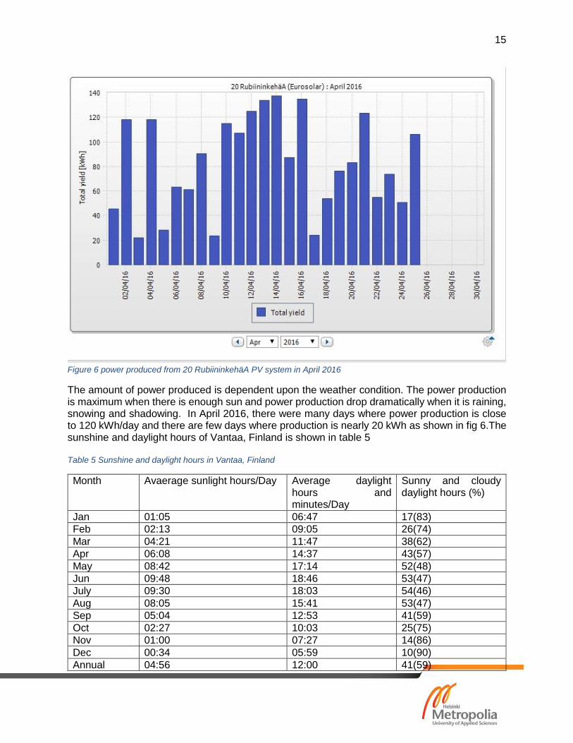
Figure 6 power produced from 20 RubiininkehäA PV system in April 2016
The amount of power produced is dependent upon the weather condition. The power production is maximum when there is enough sun and power production drop dramatically when it is raining, snowing and shadowing. In April 2016, there were many days where power production is close to 120 kWh/day and there are few days where production is nearly 20 kWh as shown in fig 6.The sunshine and daylight hours of Vantaa, Finland is shown in table 5 Table 5 Sunshine and daylight hours in Vantaa, Finland
Month Avaerage sunlight hours/Day Average daylight hours and minutes/Day
Sunny and cloudy daylight hours (%)
Jan 01:05 06:47 17(83)
Feb 02:13 09:05 26(74)
Mar 04:21 11:47 38(62)
Apr 06:08 14:37 43(57)
May 08:42 17:14 52(48)
Jun 09:48 18:46 53(47)
July 09:30 18:03 54(46)
Aug 08:05 15:41 53(47)
Sep 05:04 12:53 41(59)
Oct 02:27 10:03 25(75)
Nov 01:00 07:27 14(86)
Dec 00:34 05:59 10(90)
Annual 04:56 12:00 41(59)
16
4.3 Energy Losses in PV System
Depending on the site, technology, sizing system and weather condition might affect performance ratio (PR). The losses are as follows,
4.3.1 Pre-module Losses
This type of losses is due to shadows, dirt, snow, reflection and tolerance of power. The
module can have tolerance up to 5 % and Losses due to snow and dust might be 2 %
and Shadow can result into loss of 80% power.
4.3.2 Module losses
Conversion and thermal losses are the modules losses. With increasing temperature, conversion losses increase. The losses due to weak radiation can be 3% to 7%.
4.3.3 System Losses
Inverter losses (4% to 15%)
Temperature losses (5% to 18%)
DC cable losses (1% to 3%)
AC cables losses (1% to 3%)
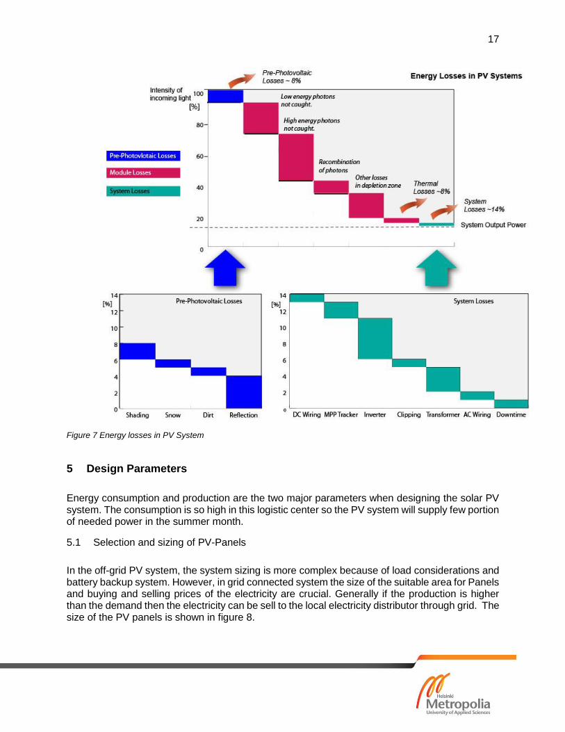
The details of energy losses in grid-connected PV System are shown in figure 7.
17
Figure 7 Energy losses in PV System
5 Design Parameters
Energy consumption and production are the two major parameters when designing the solar PV system. The consumption is so high in this logistic center so the PV system will supply few portion of needed power in the summer month.
5.1 Selection and sizing of PV-Panels
In the off-grid PV system, the system sizing is more complex because of load considerations and battery backup system. However, in grid connected system the size of the suitable area for Panels and buying and selling prices of the electricity are crucial. Generally if the production is higher than the demand then the electricity can be sell to the local electricity distributor through grid. The size of the PV panels is shown in figure 8.
18
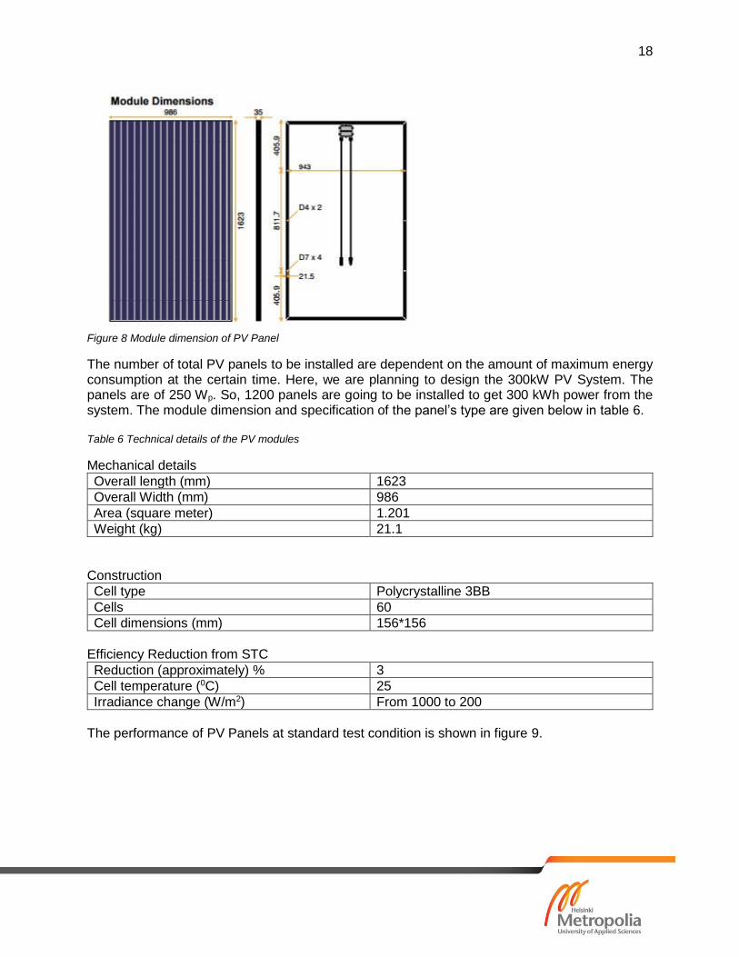
Figure 8 Module dimension of PV Panel
The number of total PV panels to be installed are dependent on the amount of maximum energy consumption at the certain time. Here, we are planning to design the 300kW PV System. The panels are of 250 Wp. So, 1200 panels are going to be installed to get 300 kWh power from the system. The module dimension and specification of the panel’s type are given below in table 6. Table 6 Technical details of the PV modules
Mechanical details
Overall length (mm) 1623
Overall Width (mm) 986
Area (square meter) 1.201
Weight (kg) 21.1
Construction
Cell type Polycrystalline 3BB
Cells 60
Cell dimensions (mm) 156*156
Efficiency Reduction from STC
Reduction (approximately) % 3
Cell temperature (0C) 25
Irradiance change (W/m2) From 1000 to 200
The performance of PV Panels at standard test condition is shown in figure 9.
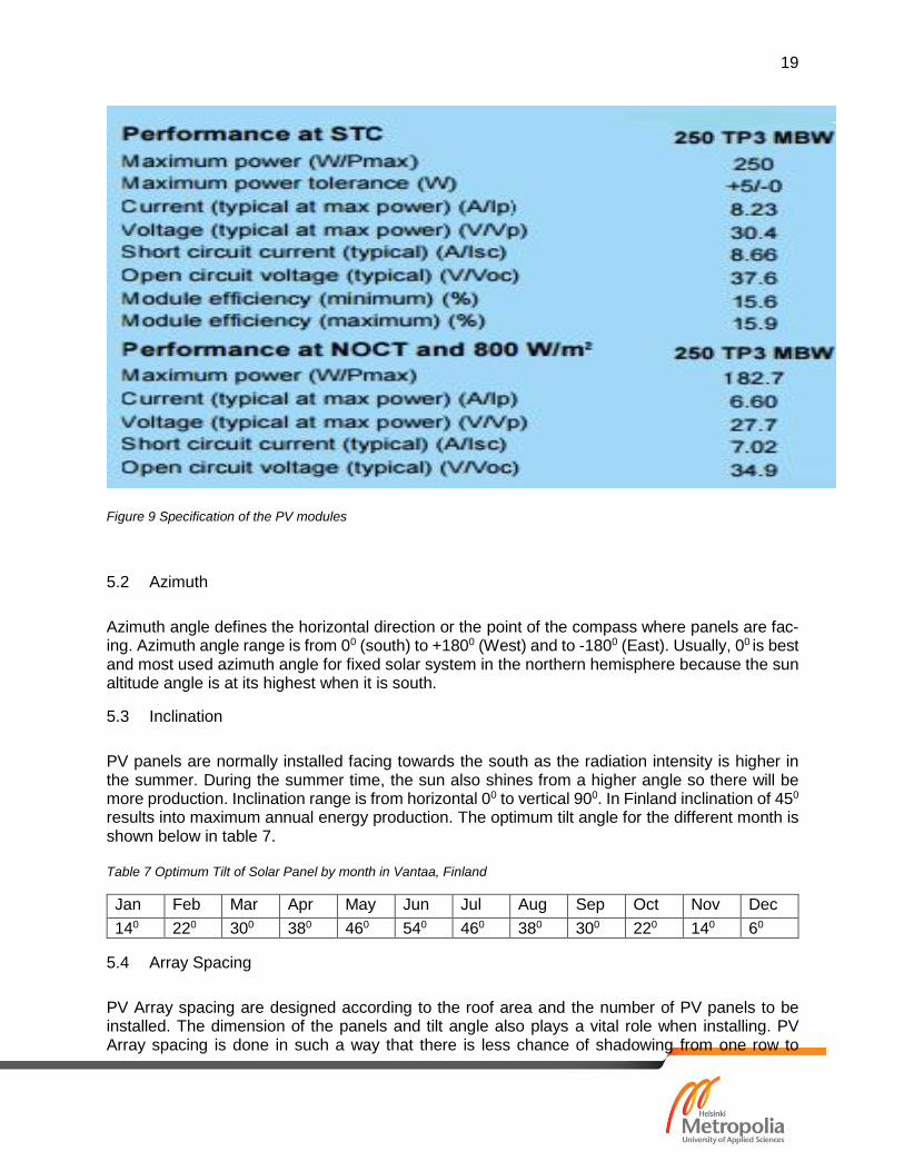
19
Figure 9 Specification of the PV modules
5.2 Azimuth
Azimuth angle defines the horizontal direction or the point of the compass where panels are fac-ing. Azimuth angle range is from 00 (south) to +1800 (West) and to -1800 (East). Usually, 00 is best and most used azimuth angle for fixed solar system in the northern hemisphere because the sun altitude angle is at its highest when it is south.
5.3 Inclination
PV panels are normally installed facing towards the south as the radiation intensity is higher in the summer. During the summer time, the sun also shines from a higher angle so there will be more production. Inclination range is from horizontal 00 to vertical 900. In Finland inclination of 450
results into maximum annual energy production. The optimum tilt angle for the different month is shown below in table 7. Table 7 Optimum Tilt of Solar Panel by month in Vantaa, Finland
Jan Feb Mar Apr May Jun Jul Aug Sep Oct Nov Dec
140 220 300 380 460 540 460 380 300 220 140 60
5.4 Array Spacing
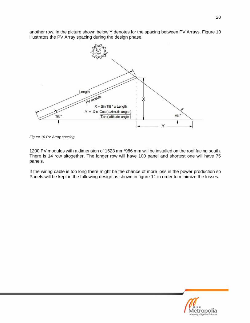
PV Array spacing are designed according to the roof area and the number of PV panels to be installed. The dimension of the panels and tilt angle also plays a vital role when installing. PV Array spacing is done in such a way that there is less chance of shadowing from one row to
20
another row. In the picture shown below Y denotes for the spacing between PV Arrays. Figure 10 illustrates the PV Array spacing during the design phase.
Figure 10 PV Array spacing
1200 PV modules with a dimension of 1623 mm*986 mm will be installed on the roof facing south. There is 14 row altogether. The longer row will have 100 panel and shortest one will have 75 panels. If the wiring cable is too long there might be the chance of more loss in the power production so Panels will be kept in the following design as shown in figure 11 in order to minimize the losses.
21
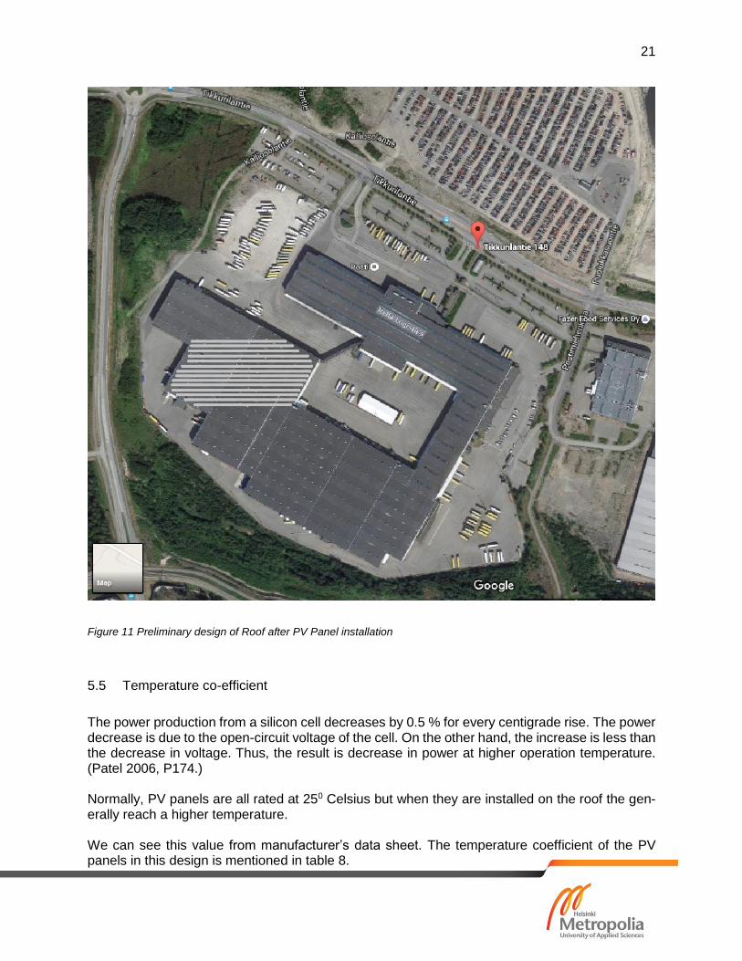
Figure 11 Preliminary design of Roof after PV Panel installation
5.5 Temperature co-efficient
The power production from a silicon cell decreases by 0.5 % for every centigrade rise. The power decrease is due to the open-circuit voltage of the cell. On the other hand, the increase is less than the decrease in voltage. Thus, the result is decrease in power at higher operation temperature. (Patel 2006, P174.) Normally, PV panels are all rated at 250 Celsius but when they are installed on the roof the gen-erally reach a higher temperature. We can see this value from manufacturer’s data sheet. The temperature coefficient of the PV panels in this design is mentioned in table 8.
22
Table 8 Temperature coefficient value at STC
Open circuit voltage (V/K) -0.125
Short circuit current (A/K) 0.00477
Maximum power (%K) -0.42
5.6 Inverter selection and manufacture type
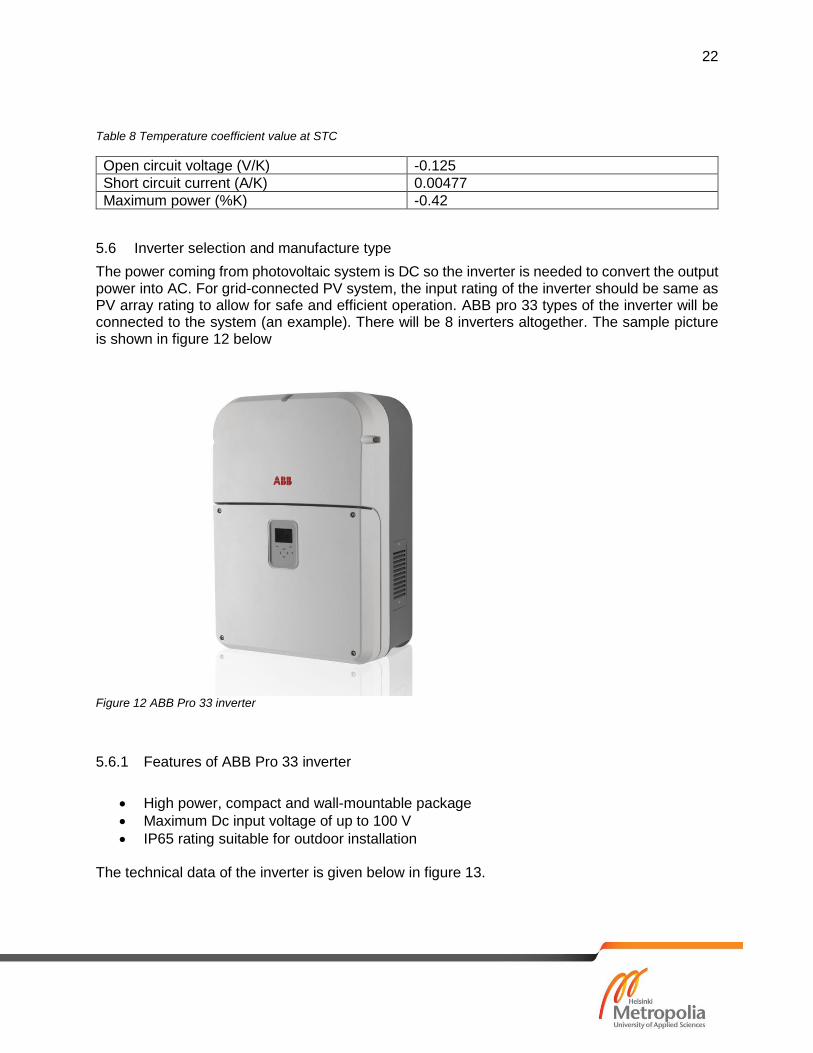
The power coming from photovoltaic system is DC so the inverter is needed to convert the output power into AC. For grid-connected PV system, the input rating of the inverter should be same as PV array rating to allow for safe and efficient operation. ABB pro 33 types of the inverter will be connected to the system (an example). There will be 8 inverters altogether. The sample picture is shown in figure 12 below
Figure 12 ABB Pro 33 inverter
5.6.1 Features of ABB Pro 33 inverter
High power, compact and wall-mountable package
Maximum Dc input voltage of up to 100 V
IP65 rating suitable for outdoor installation The technical data of the inverter is given below in figure 13.
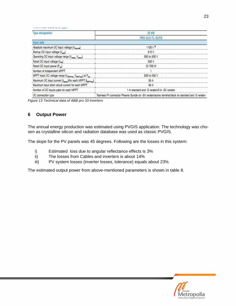
23
Figure 13 Technical data of ABB pro 33 inverters
6 Output Power
The annual energy production was estimated using PVGIS application. The technology was cho-sen as crystalline silicon and radiation database was used as classic PVGIS. The slope for the PV panels was 45 degrees. Following are the losses in this system:
i) Estimated loss due to angular reflectance effects is 3%
ii) The losses from Cables and inverters is about 14%
iii) PV system losses (inverter losses, tolerance) equals about 23%
The estimated output power from above-mentioned parameters is shown in table 8.
24
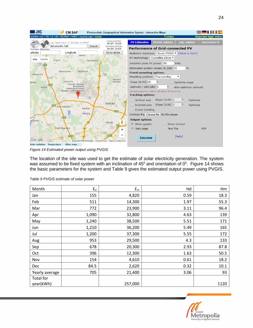
Figure 14 Estimated power output using PVGIS
The location of the site was used to get the estimate of solar electricity generation. The system was assumed to be fixed system with an inclination of 450 and orientation of 00. Figure 14 shows the basic parameters for the system and Table 9 gives the estimated output power using PVGIS. Table 9 PVGIS estimate of solar power
Month Ed Em Hd Hm
Jan 155 4,820 0.59 18.3
Feb 511 14,300 1.97 55.3
Mar 772 23,900 3.11 96.4
Apr 1,090 32,800 4.63 139
May 1,240 38,500 5.51 171
Jun 1,210 36,200 5.49 165
Jul 1,200 37,300 5.55 172
Aug 953 29,500 4.3 133
Sep 678 20,300 2.93 87.8
Oct 396 12,300 1.63 50.5
Nov 154 4,610 0.61 18.2
Dec 84.5 2,620 0.32 10.1
Yearly average 705 21,400 3.06 93
Total for year(kWh) 257,000 1120
25
Where, Ed: Average daily electricity production from the given system (kWh) Em: Average monthly electricity production from the given system (kWh) Hd: Average daily sum of global irradiation per square meter received by the modules of the given system (kWh/m2) Hm: Average sum of global irradiation per square meter received by the modules of the given system (kWh/m2)
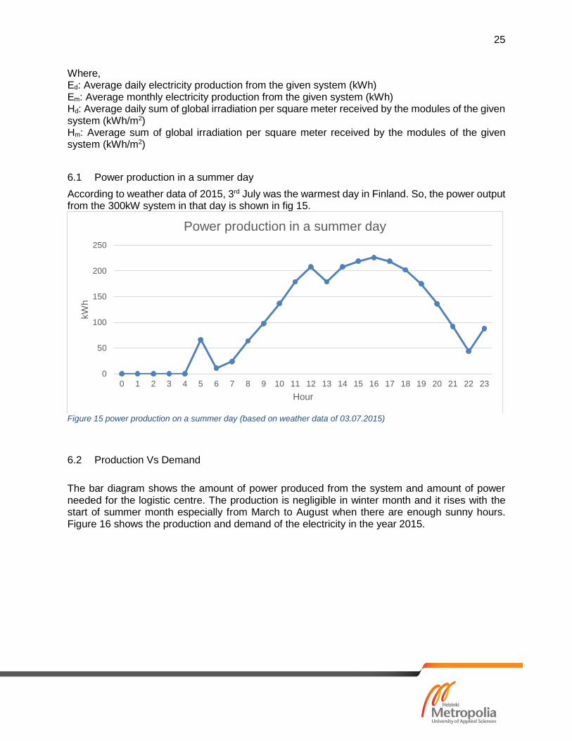
6.1 Power production in a summer day
According to weather data of 2015, 3rd July was the warmest day in Finland. So, the power output from the 300kW system in that day is shown in fig 15.
Figure 15 power production on a summer day (based on weather data of 03.07.2015)
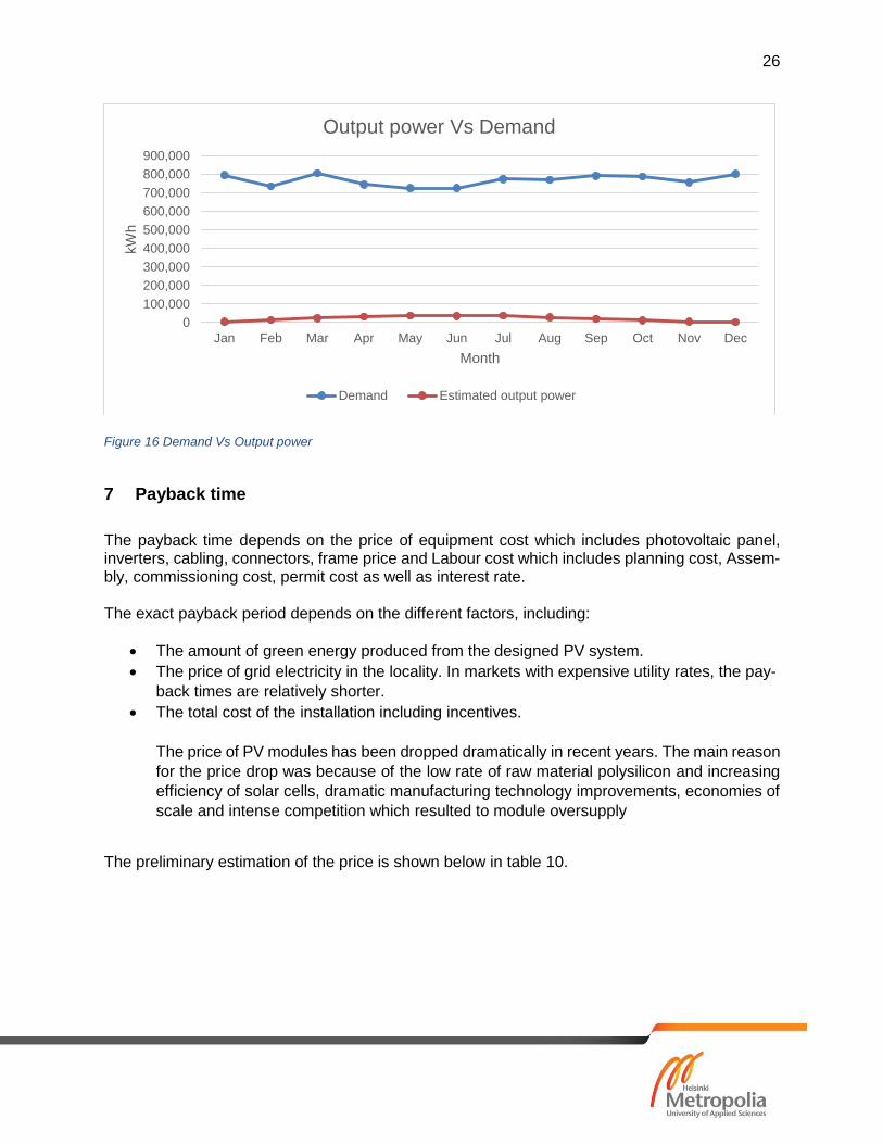
6.2 Production Vs Demand
The bar diagram shows the amount of power produced from the system and amount of power needed for the logistic centre. The production is negligible in winter month and it rises with the start of summer month especially from March to August when there are enough sunny hours. Figure 16 shows the production and demand of the electricity in the year 2015.
0
50
100
150
200
250
0 1 2 3 4 5 6 7 8 9 10 11 12 13 14 15 16 17 18 19 20 21 22 23
kW
h
Hour
Power production in a summer day
26
Figure 16 Demand Vs Output power
7 Payback time
The payback time depends on the price of equipment cost which includes photovoltaic panel, inverters, cabling, connectors, frame price and Labour cost which includes planning cost, Assem-bly, commissioning cost, permit cost as well as interest rate. The exact payback period depends on the different factors, including:
The amount of green energy produced from the designed PV system.
The price of grid electricity in the locality. In markets with expensive utility rates, the pay-
back times are relatively shorter.
The total cost of the installation including incentives.
The price of PV modules has been dropped dramatically in recent years. The main reason
for the price drop was because of the low rate of raw material polysilicon and increasing
efficiency of solar cells, dramatic manufacturing technology improvements, economies of
scale and intense competition which resulted to module oversupply
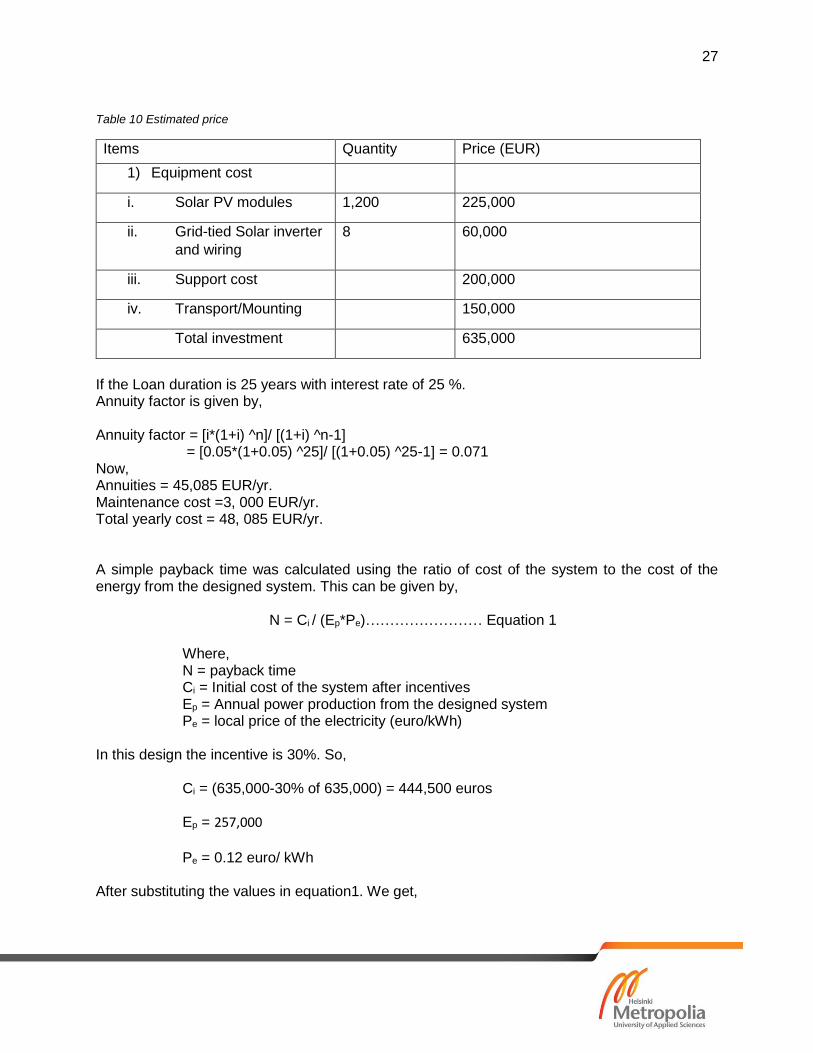
The preliminary estimation of the price is shown below in table 10.
0
100,000
200,000
300,000
400,000
500,000
600,000
700,000
800,000
900,000
Jan Feb Mar Apr May Jun Jul Aug Sep Oct Nov Dec
kW
h
Month
Output power Vs Demand
Demand Estimated output power
27
Table 10 Estimated price
Items Quantity Price (EUR)
1) Equipment cost
i. Solar PV modules 1,200 225,000
ii. Grid-tied Solar inverter
and wiring
8 60,000
iii. Support cost 200,000
iv. Transport/Mounting 150,000
Total investment 635,000
If the Loan duration is 25 years with interest rate of 25 %. Annuity factor is given by, Annuity factor = [i*(1+i) ^n]/ [(1+i) ^n-1] = [0.05*(1+0.05) ^25]/ [(1+0.05) ^25-1] = 0.071 Now, Annuities = 45,085 EUR/yr. Maintenance cost =3, 000 EUR/yr. Total yearly cost = 48, 085 EUR/yr. A simple payback time was calculated using the ratio of cost of the system to the cost of the energy from the designed system. This can be given by, N = Ci / (Ep*Pe)…………………… Equation 1 Where, N = payback time Ci = Initial cost of the system after incentives Ep = Annual power production from the designed system Pe = local price of the electricity (euro/kWh) In this design the incentive is 30%. So,
Ci = (635,000-30% of 635,000) = 444,500 euros Ep = 257,000 Pe = 0.12 euro/ kWh After substituting the values in equation1. We get,
28
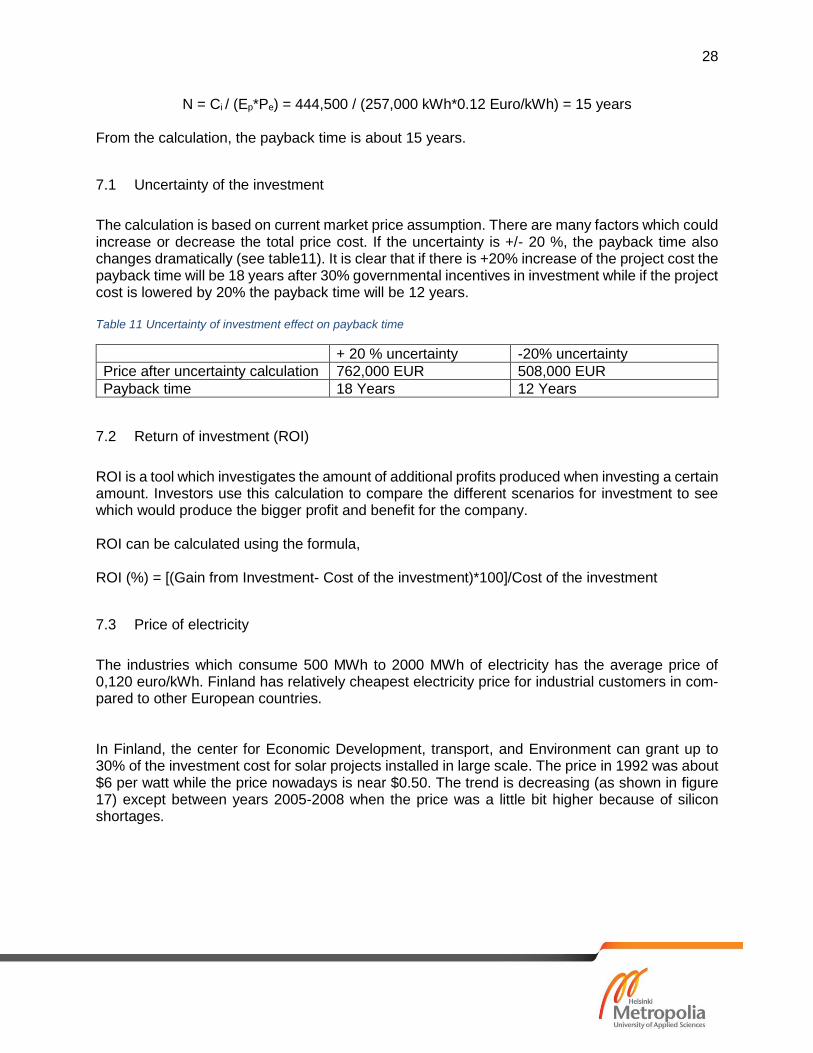
N = Ci / (Ep*Pe) = 444,500 / (257,000 kWh*0.12 Euro/kWh) = 15 years From the calculation, the payback time is about 15 years.
7.1 Uncertainty of the investment
The calculation is based on current market price assumption. There are many factors which could increase or decrease the total price cost. If the uncertainty is +/- 20 %, the payback time also changes dramatically (see table11). It is clear that if there is +20% increase of the project cost the payback time will be 18 years after 30% governmental incentives in investment while if the project cost is lowered by 20% the payback time will be 12 years. Table 11 Uncertainty of investment effect on payback time
+ 20 % uncertainty -20% uncertainty
Price after uncertainty calculation 762,000 EUR 508,000 EUR
Payback time 18 Years 12 Years
7.2 Return of investment (ROI)
ROI is a tool which investigates the amount of additional profits produced when investing a certain amount. Investors use this calculation to compare the different scenarios for investment to see which would produce the bigger profit and benefit for the company. ROI can be calculated using the formula, ROI (%) = [(Gain from Investment- Cost of the investment)*100]/Cost of the investment
7.3 Price of electricity
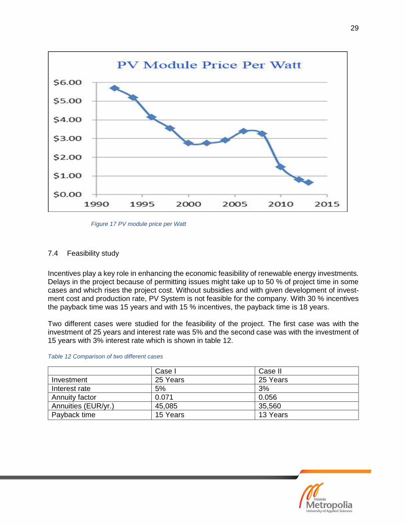
The industries which consume 500 MWh to 2000 MWh of electricity has the average price of 0,120 euro/kWh. Finland has relatively cheapest electricity price for industrial customers in com-pared to other European countries. In Finland, the center for Economic Development, transport, and Environment can grant up to 30% of the investment cost for solar projects installed in large scale. The price in 1992 was about $6 per watt while the price nowadays is near $0.50. The trend is decreasing (as shown in figure 17) except between years 2005-2008 when the price was a little bit higher because of silicon shortages.
29
Figure 17 PV module price per Watt
7.4 Feasibility study
Incentives play a key role in enhancing the economic feasibility of renewable energy investments. Delays in the project because of permitting issues might take up to 50 % of project time in some cases and which rises the project cost. Without subsidies and with given development of invest-ment cost and production rate, PV System is not feasible for the company. With 30 % incentives the payback time was 15 years and with 15 % incentives, the payback time is 18 years. Two different cases were studied for the feasibility of the project. The first case was with the investment of 25 years and interest rate was 5% and the second case was with the investment of 15 years with 3% interest rate which is shown in table 12. Table 12 Comparison of two different cases
Case I Case II
Investment 25 Years 25 Years
Interest rate 5% 3%
Annuity factor 0.071 0.056
Annuities (EUR/yr.) 45,085 35,560
Payback time 15 Years 13 Years
30
8 Conclusions
Energy produced from renewable energy sources like solar energy is getting popular as the en-ergy produced is green energy and there are no greenhouse gas emissions. At the same time, the energy produced is free. Because of more emphasis on renewable energy, subsidies when installing the system, the PV installation is in increasing trend and payback time is becoming shorter. The operating and maintenance costs for PV panels are negligible, compared to the costs of other renewable energy systems. There is a high possibility of obtaining benefits from on-grid solar systems when the consumption is less so that surplus electricity can be sold to the local electricity supply. In some countries, the power produced from renewable energy sources like wind energy, hydro energy, solar energy etc. have higher feed-in tariff rates. In this design, PV panels will be installed on the roof of the property. So, no additional land is needed. Because of increasing trend of electricity price, carbon trade issues and clean develop-ment mechanisms, this type of a system will play a key role in achieving the EU’s target for 20% of renewable energy supply by the year 2020. The payback time for the system is estimated to be 12-15 years. Due to the uncertainty price in the investment the payback time vary significantly. Estimated lifetime of PV panel is more than 25 years, so in longer run system would bring economical benefit.
31
References
[1] "Sustainability Report," Posti Group Oyj, 2015.
[2] H. Timo, "The role and opportunities for solar energy in Finland and Europe," VTT Oy, Espoo, 2015.
[3] H. Teemu, "PV System Design and feasibility study for Juhannuslehto Business Park," SAMK, Satakunta, December 2013.
[4] S. J. Brunner, "Model to Calculate PV Array Altitude and Azimuth Angles to Maximize Energy and Demand Revenues from," Brendle Group, Fort Collins.
[5] A. Christensen, "Bright future for solar energy in the north," ScienceNordic, 2012.
[6] M. Boxwell, "Solar Electricity Handbook 2016 Edition," Greenstream Publishing, 2016.
[7] "Naps System," Naps solar system, [Online]. Available: http://www.napssystems.com/wordpress/wp-content/uploads/2014/02/DS_SAANA245-255TP3MBW_EN_mail.pdf. [Accessed 02 05 2016].
[8] Suri M, Huld T.A and Dunlop E.D Ossenbrink H.A, "Potential os solar electricity generation in the European Union member states and candidate countries," Solar Energy, vol. 81, pp. 1295-1305, 2007.
[9] "Green Rhino Energy Ltd.," 2013. [Online]. Available: http://www.greenrhinoenergy.com/solar/technologies/pv_energy_yield.php. [Accessed 02 05 2016].
[10] ABB, 2015. [Online]. Available: www.abb.com/solarinverters. [Accessed 01 05 2016].
[11] "Leonics," [Online]. Available: http://www.leonics.com/support/article2_12j/articles2_12j_en.php. [Accessed 25 April 2016].
[12] a. Brentley, Direct Energy Solar, 2014. [Online]. Available: http://www.directenergysolar.com/blog/post/what-is-the-average-payback-period-of-a-solar-installation/. [Accessed 02 05 2015].
[13] G. Davis, "A guide to photovoltaic system and installation," California Energy Commission, California, June 2001.
[14] Roos, Carolyn, "Solar Electric System Design, Operation and Installation," Washington State University, Washington, 2009.
[15] T. Huld, "Global irradiation and solar electricity potential," European Commission.
32
[16] "PV Array row spacing," Clean Energy Council, 2010.
[17] K. P. Lall, S. K. Sahoo and S. P. Karthikeyan, "Grid-Connected Solar PV System," Electrical India, Tamil Nadu, 2015.
[18] E. Pihlakivi, "Potential of Solar Energy in Finland," Turun Ammattikorkeakoulu, Turku, 2015.
[19] J. Meyer, "Solar Electricity Utilization in Finland," Metropolia UAS, Helsinki, 2015.
[20] "PVSYST Photovaltic software," [Online]. Available: http://www.pvsyst.com/en/download. [Accessed 03 05 2016].
[21] "Green Energy and Technology," [Online]. Available: http://www.greentech.cdit.org/index.php/component/content/article/79-solar/90-solar-pv-system. [Accessed 03 05 2016].
[22] "ClimaTemps.com," [Online]. Available: http://www.helsinki.climatemps.com/sunlight.php. [Accessed 02 05 2016].
[23] "HELEN," Helsingin Energia, [Online]. Available: https://www.helen.fi/sahko/kodit/aurinkovoimalat/suvilahti/. [Accessed 28 04 2016].
33
9 Appendices
9.1 Electricity consumption in summer day and winter day
34
9.2 Global irradiation and PV potential in Europe
35
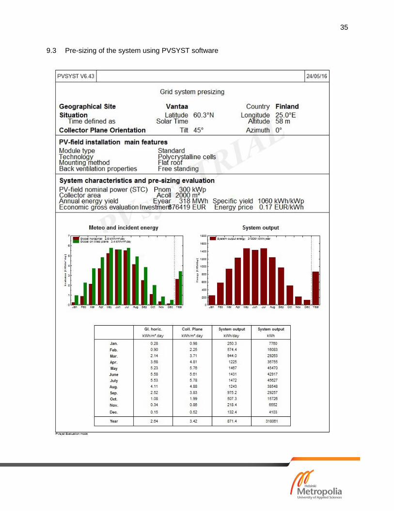
9.3 Pre-sizing of the system using PVSYST software
36
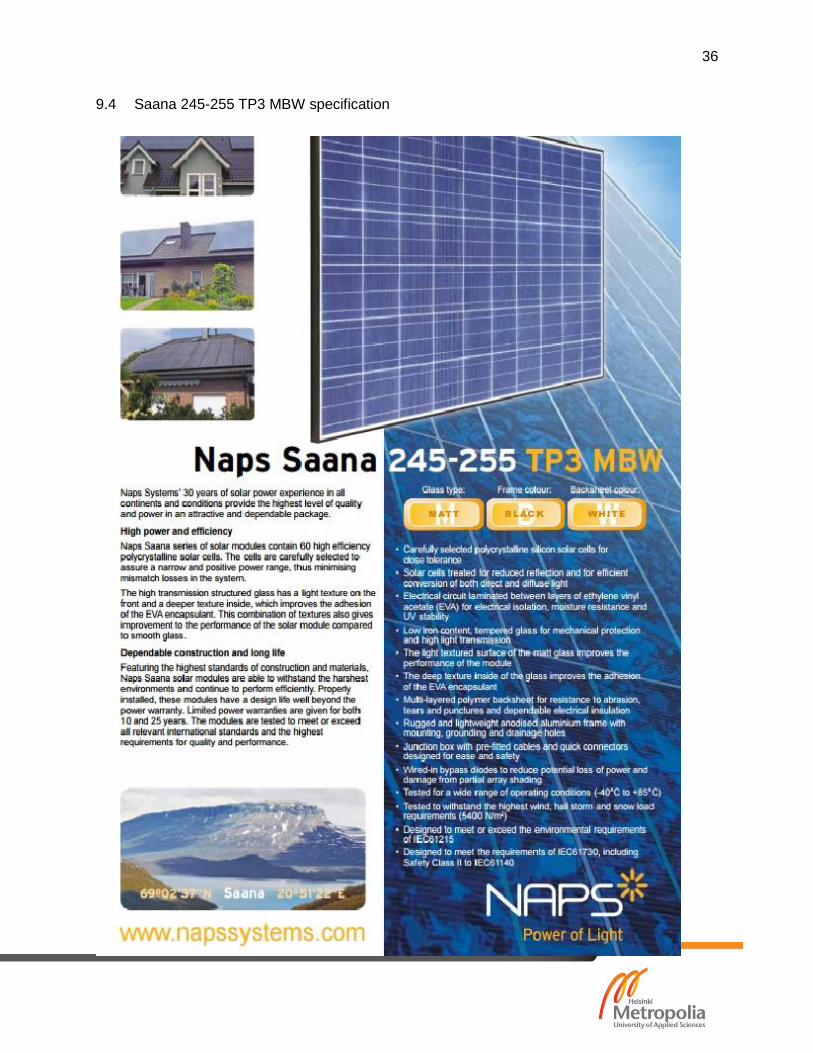
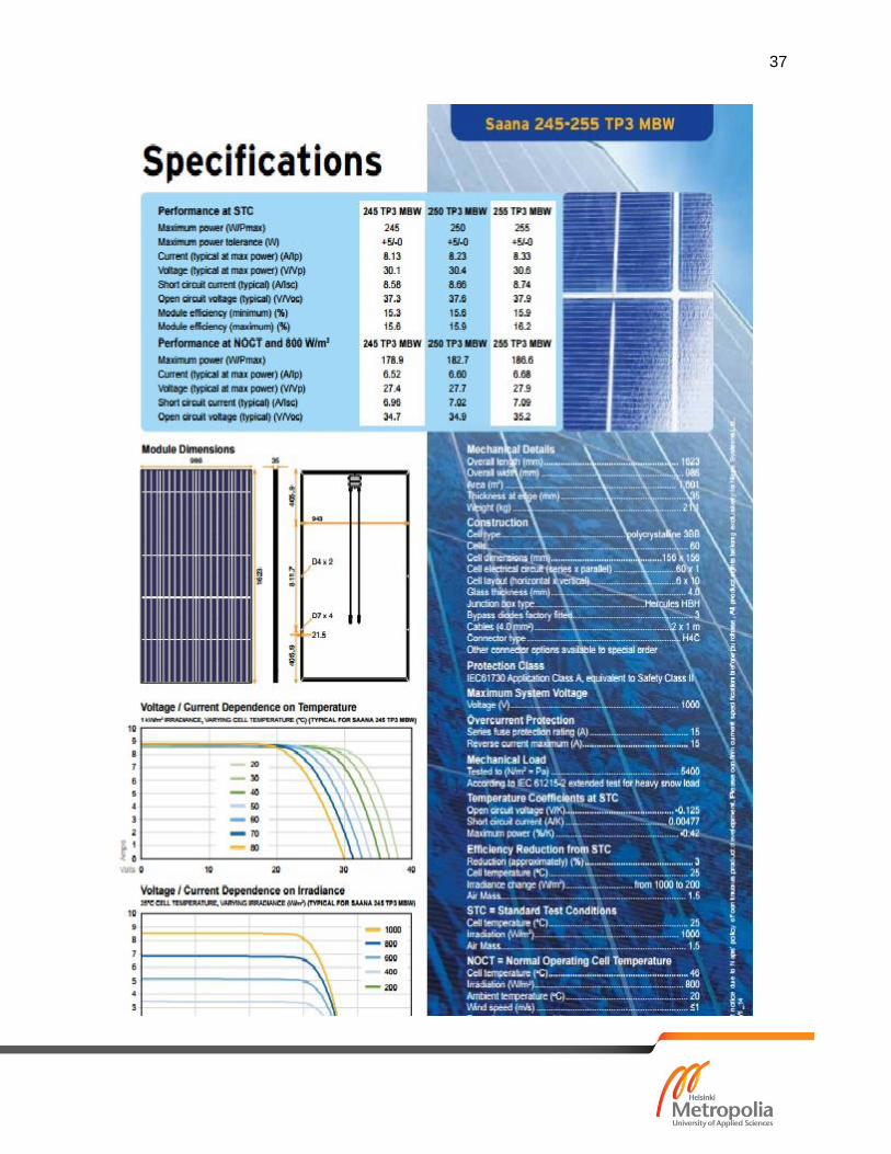
9.4 Saana 245-255 TP3 MBW specification
37